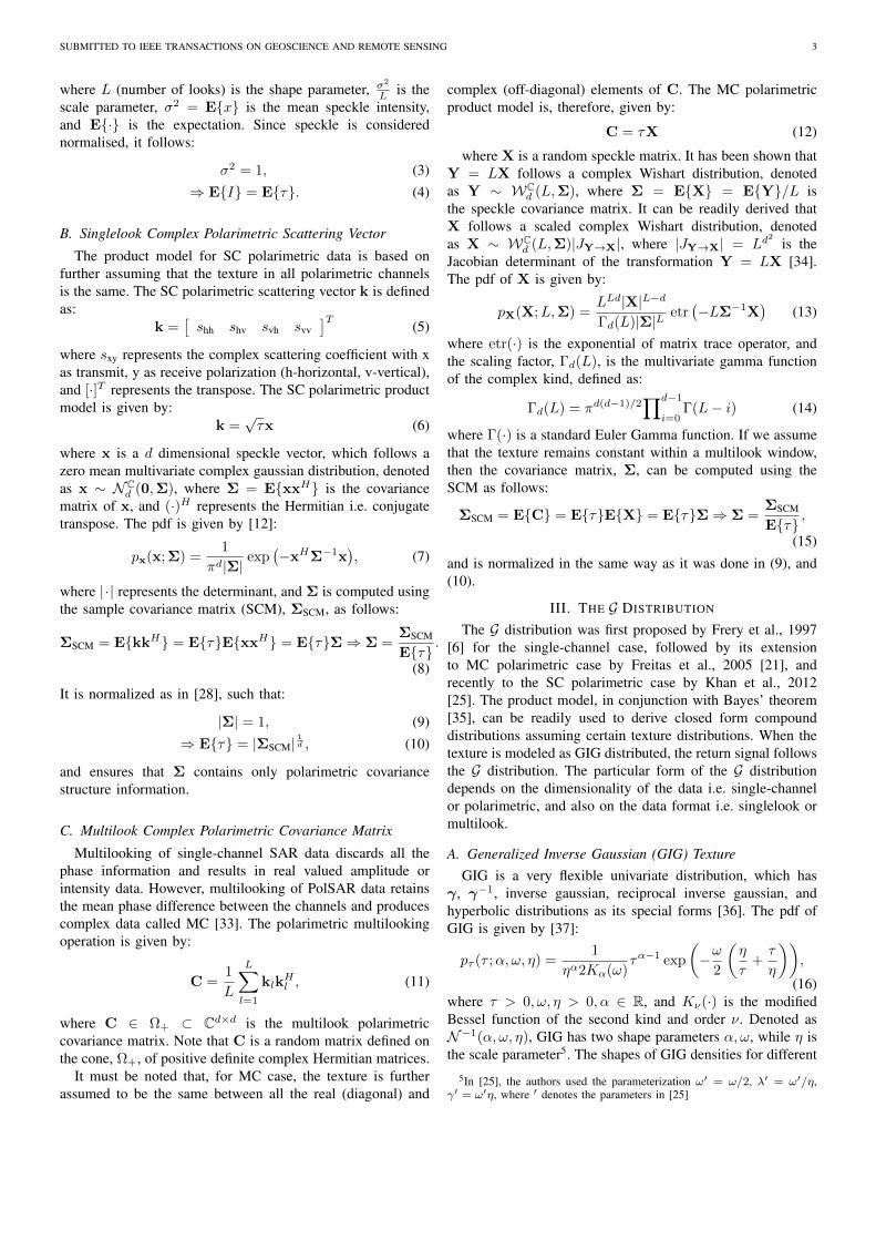
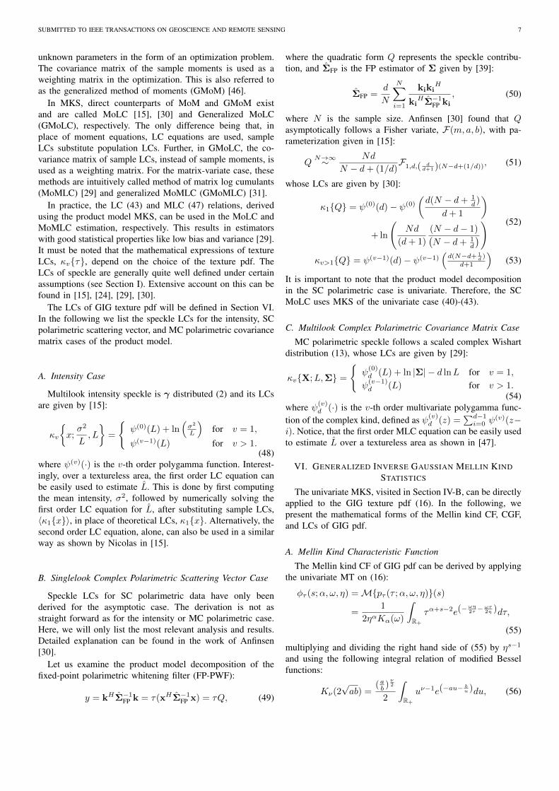
SUBMITTED TO IEEE TRANSACTIONS ON GEOSCIENCE AND REMOTE SENSING 1

Application of Mellin Kind Statistics toPolarimetric G Distribution for SAR Data

Salman Khan, Student Member, IEEE, and Raffaella Guida, Member, IEEE

Abstract—The K distribution can be arguably regarded asone of most successful and widely used models for radar data.However, in the last two decades we have seen tremendous growthin even more accurate modeling of radar statistics. In this regard,the relatively recent G0 distribution filled some deficiencies leftunaccounted by the K model. The G0 model actually resulted asa special case of a more general model; the G distribution, whichalso has the K model as its special form. Singlelook complex(SC) and multilook complex (MC) polarimetric extensions ofthese models (and many others) have also been proposed inthis prolific era. Unfortunately, statistical analysis using thepolarimetric G distribution remained limited, primarily becauseof more complicated parameter estimation. In this paper, theauthors have analyzed the G model for its parameter estimationusing state-of-the-art univariate and matrix-variate Mellin KindStatistics (MKS). The outcome is a class of estimators basedon Method of Log Cumulants (MoLC), and Method of MatrixLog Cumulants (MoMLC). These estimators show superiorperformance characteristics for product model distributions likethe G model. Diverse regions in TerraSAR-X polarimetric SAR(PolSAR) data have also been statistically analyzed using the Gmodel with its new and old estimators. Formal Goodness-of-fit(GoF) testing, based on MKS theory, has been used to assess thefitting accuracy between different estimators and also betweenG, K, G0, and Kummer-U models.

Index Terms—synthetic aperture radar (SAR), polarimet-ric G distribution, generalized inverse gaussian (GIG), Fisher,Kummer-U distribution, radar statistics, Mellin kind statistics,Method of log cumulants, numerical differentiation

I. INTRODUCTION

OBJECTS illuminated by light from a highly coherentcontinuous wave laser are readily observed to acquire

a peculiar granular appearance called speckle. The origins ofspeckle were promptly recognized by early researchers in thelaser field [1]. Direct analogs of speckle are found in all typesof coherent imagery including SAR. One intuitive explanationof speckle formation in coherent imagery is that the reflectedwaves from different scatterers arrive back at the source withrandom delays. The incoherent addition of these out-of-phasereflected components results in chaotic bright and dark spots[2]. Due to the random nature of speckle, SAR imagery isinherently probabilistic. Consequently, statistical modeling ofSAR data is a fundamental aspect of SAR image analysis.

Let us make the following assumptions 1) a large number ofscatterers are present in a resolution cell, 2) the slant range ismuch larger than the wavelength, 3) the amplitude and phasefrom individual scatterers are independent and identicallydistributed random variables, and 4) the phase is uniformly dis-tributed. Then, according to central limit theorem, the complexreturn from a singlelook complex (SC) SAR image followsa zero mean circular complex gaussian distribution [3]. The

gaussian model also includes the corresponding distributionsof singlelook (and multilook) amplitude and intensity returns.It can be readily derived, that the corresponding singlelook am-plitude is Rayleigh distributed, while the singlelook intensity isexponentially distributed [3]. For multilook data, the amplitudeis square root of gamma distributed, while the intensity isgamma distributed [3]–[5]. It has been experimentally verifiedthat the gaussian model generally provides a good fit tosinglelook and multilook SAR data specially when the imageroughness is relatively low and a large number of scatterers arepresent. As the resolution increases, the assumption of a largenumber of scatterers in a resolution cell is not always true. Ithas also been noted that in certain areas of a SAR image thestatistics deviate from the gaussian assumption e.g. urban areasshow considerable non-gaussianity [6], [7]. Similarly, naturalareas like forests and rough sea surface are also known toexhibit non-gaussianity [8], [9].

Many distributions have been proposed to model non-gaussianity for single-channel SAR data e.g Weibull, Log-normal, Nakagami-Rice [7]. However, some distributions havebeen derived for single-channel as well as multi-channel(PolSAR) data using a doubly stochastic product model. Thismodel provides a framework to generate multivariate non-gaussian distributions by assuming that the observed signalis a product of a gaussian speckle random variate and a non-gaussian texture random variate. A special case of this model,called scalar texture product model, has been extensivelyand successfully used to model non-gaussianity for single-channel and more importantly PolSAR data. This modelassumes that the texture random variate is restricted to apositive scalar random variable. The extension to PolSARdata is not straightforward as noted in [4], and mandatescertain assumptions. Recently, some research has been donein multi-texture modeling as well [10], [11]. In this paper,we will restrict ourselves to the scalar texture case as ourmethods are scalable to certain multi-texture cases. In contrastto contemporary literature, we will use the terms textured andtextureless areas when we refer to areas with non-gaussian andgaussian statistics, respectively1.

Singlelook PolSAR speckle can be shown to follow amultivariate zero mean complex gaussian distribution [12].The gaussian counterpart for the multilook PolSAR case isthe matrix-variate scaled complex Wishart distribution [12].Both these models have been experimentally verified on realPolSAR data [13], [14]. In the context of scalar textureproduct model, different distributions for the texture random

1gaussian and non-gaussian areas have been commonly referred to ashomogeneous and heterogeneous areas, respectively. We refrain from thisnomenclature as some homogeneous areas also show non-gaussianity.

SUBMITTED TO IEEE TRANSACTIONS ON GEOSCIENCE AND REMOTE SENSING 2

variable will result in different expressions for the resultingcompound distribution. The choice of texture distribution canbe based on physical characteristics, empirical evidence, orsimply flexibility of fitting real data. Some of the importanttexture distributions proposed in literature are gamma (γ),inverse gamma (γ−1), Generalized Inverse Gaussian (GIG),Fisher2 (F), beta (β), and inverse beta (β−1) with the resultingcompound distributions K, G0, G, Kummer-U , W , and M,respectively [6], [18]–[24]. All the compound distributionshave certain special functions in their closed form expressions.Generally, the less complicated the special function, and themore flexible the distribution shape, the better. In this regard,the G0 distribution has been shown to be very flexible andcomputationally inexpensive, capable of modeling varyingdegrees of texture [6], [21]. However, real PolSAR data invarious frequency bands often requires more flexibility thanthe G0 model [22]–[25]. This paper concentrates on the Gdistribution, a very flexible model, derived assuming GIGtexture, with K and G0 distributions as its well known specialcases [6], [21], [25]. Recently, it has also been shown bythe authors that this model is at least as flexible as theKummer-U distribution [11]. It is also pertinent to mentioned,that the G distribution has another special case referred toas the harmonic G distribution, denoted as Gh, proposed forsingle-channel case in [26], and extended to model multilookcomplex (MC) polarimetric data in [27], and SC polarimetricdata in [28]3.

Efficient parameter estimation of the polarimetric G dis-tribution has been a hard computational task [6], [21], [25].One alternative is to estimate parameters on each individualchannel, and average the so called mono-pol estimates toobtain estimates for the polarimetric distribution (See SectionIII). Such mono-pol estimators have been shown to be inferior,in terms of estimator bias and variance, to polarimetric estima-tors4 [29]. An important development in this regard has beenthe MoLC for mono-pol parameter estimation [15], which hasbeen extended to polarimetric estimators in [29], [30]. TheMoLC estimation has been shown to be suitable and intuitivefor compound distributions (mono-pol and polarimetric) aris-ing from the doubly stochastic product model [15], [24], [29],[30].

In this paper, we apply the MoLC estimation to the po-larimetric singlelook and multilook G distribution, extendingour preliminary work presented in [11]. Then, we compare thenew polarimetric estimator to two other somewhat traditionalestimators: 1) based on mono-pol fractional moments, and2) numerical Maximum Likelihood Estimation (MLE) [25],extended to the multilook case. Further, we apply all the above

2It is relevant to mention, that the F distribution, proposed by Nicolas, 2002[15], [16] to model texture and also intensity [17], is only the G0I intensitydistribution parameterised by its mean, proposed earlier by Frery et al., 1997[6]. Both result from the product of γ and γ−1 distributed random variables.However, the latter was proposed only for intensity return, while the formermodeled both texture and intensity.

3In [28], the SC polarimetric Gh distribution was referred to as multivariatenormal inverse gaussian (MNIG) distribution.

4Polarimetric estimators utilize fully polarimetric information in the formof covariance structure between polarimetric channels for estimation unlikemono-pol estimators.

mentioned estimators for G distribution to real PolSAR data.Also, we apply the polarimetric MoLC estimators for G0, K,and Kummer-U distributions to real PolSAR data [29], [30].Finally, we compute a formal χ2 distributed Goodness-of-Fit(GoF) test statistic, based on multiple log cumulants and spe-cially designed for polarimetric data [31]. This facilitates theGoF comparison between different estimators and distributionson real data.

The rest of the paper has been organized as follows. SectionII elaborates the scalar texture product model for single-channel intensity and polarimetric SC and MC SAR dataformats. Section III presents the G distribution correspondingto these formats. Previously known estimators of the G dis-tribution are also listed in Section III. In Section IV, a briefreview of MKS is documented as an essential prerequisite toMoLC. Section V covers the MoLC for the above mentionedSAR data formats. Univariate MKS theory has been appliedto GIG pdf in Section VI. Close form expressions for logcumulants of G distribution are listed in Section VII. In SectionVIII, the proposed estimator’s accuracy and precision arecompared to those of the known estimators. Section IX brieflydescribes the GoF framework. Section X shows the applicationto real PolSAR data. Finally, in Section XI some conclusionsare drawn.

II. THE SCALAR TEXTURE PRODUCT MODEL

The scalar texture product model, as mentioned before,states that the observed signal is a product of a positive scalartexture random variable and a speckle random variate. The for-mer is analogous to the natural spatial variation of radar crosssection, which generally varies even for thematically similarpixels. It is also assumed that the texture is spatially varyingon a larger scale than speckle. The product model takesdifferent forms for SC and MC PolSAR data formats. This isbecause MC data contains all the second order moments of thescattering coefficients of SC data within a multilook window[32]. Hence, the statistics of these data formats are different.In the following, we assume τ to represent a positive scalartexture random variable with an unspecified pdf pτ (τ). Wealso assume that the speckle random variate is normalized sothat the scale is transferred to the texture variable, and henceits scale parameter must be separately estimated.

A. Single-channel Intensity Return

First we consider the case of mono-pol intensity return. Theproduct model is thus given by:

I = τx (1)

where I is the intensity return, and x is the speckle intensityrandom variable. The pdf of x is exponentially distributedfor singlelook case and γ distributed for multilook case.As exponential distribution is a special form of the γ, it issufficient to show only the distribution of multilook intensityspeckle [5]:

px

(x;L,

σ2

L

)=

(L

σ2

)LxL−1

Γ(L)exp

(−Lxσ2

), (2)

SUBMITTED TO IEEE TRANSACTIONS ON GEOSCIENCE AND REMOTE SENSING 3

where L (number of looks) is the shape parameter, σ2

L is thescale parameter, σ2 = Ex is the mean speckle intensity,and E· is the expectation. Since speckle is considerednormalised, it follows:

σ2 = 1, (3)⇒ EI = Eτ. (4)

B. Singlelook Complex Polarimetric Scattering Vector

The product model for SC polarimetric data is based onfurther assuming that the texture in all polarimetric channelsis the same. The SC polarimetric scattering vector k is definedas:

k =[shh shv svh svv

]T(5)

where sxy represents the complex scattering coefficient with xas transmit, y as receive polarization (h-horizontal, v-vertical),and [·]T represents the transpose. The SC polarimetric productmodel is given by:

k =√τx (6)

where x is a d dimensional speckle vector, which follows azero mean multivariate complex gaussian distribution, denotedas x ∼ NC

d (0,Σ), where Σ = ExxH is the covariancematrix of x, and (·)H represents the Hermitian i.e. conjugatetranspose. The pdf is given by [12]:

px(x; Σ) =1

πd|Σ|exp

(−xHΣ−1x

), (7)

where |·| represents the determinant, and Σ is computed usingthe sample covariance matrix (SCM), ΣSCM, as follows:

ΣSCM = EkkH = EτExxH = EτΣ⇒ Σ =ΣSCM

Eτ.

(8)

It is normalized as in [28], such that:

|Σ| = 1, (9)⇒ Eτ = |ΣSCM|

1d , (10)

and ensures that Σ contains only polarimetric covariancestructure information.

C. Multilook Complex Polarimetric Covariance Matrix

Multilooking of single-channel SAR data discards all thephase information and results in real valued amplitude orintensity data. However, multilooking of PolSAR data retainsthe mean phase difference between the channels and producescomplex data called MC [33]. The polarimetric multilookingoperation is given by:

C =1

L

L∑l=1

klkHl , (11)

where C ∈ Ω+ ⊂ Cd×d is the multilook polarimetriccovariance matrix. Note that C is a random matrix defined onthe cone, Ω+, of positive definite complex Hermitian matrices.

It must be noted that, for MC case, the texture is furtherassumed to be the same between all the real (diagonal) and

complex (off-diagonal) elements of C. The MC polarimetricproduct model is, therefore, given by:

C = τX (12)

where X is a random speckle matrix. It has been shown thatY = LX follows a complex Wishart distribution, denotedas Y ∼ WC

d (L,Σ), where Σ = EX = EY/L isthe speckle covariance matrix. It can be readily derived thatX follows a scaled complex Wishart distribution, denotedas X ∼ WC

d (L,Σ)|JY→X|, where |JY→X| = Ld2

is theJacobian determinant of the transformation Y = LX [34].The pdf of X is given by:

pX(X;L,Σ) =LLd|X|L−d

Γd(L)|Σ|Letr(−LΣ−1X

)(13)

where etr(·) is the exponential of matrix trace operator, andthe scaling factor, Γd(L), is the multivariate gamma functionof the complex kind, defined as:

Γd(L) = πd(d−1)/2∏d−1

i=0Γ(L− i) (14)

where Γ(·) is a standard Euler Gamma function. If we assumethat the texture remains constant within a multilook window,then the covariance matrix, Σ, can be computed using theSCM as follows:

ΣSCM = EC = EτEX = EτΣ⇒ Σ =ΣSCM

Eτ,

(15)

and is normalized in the same way as it was done in (9), and(10).

III. THE G DISTRIBUTION

The G distribution was first proposed by Frery et al., 1997[6] for the single-channel case, followed by its extensionto MC polarimetric case by Freitas et al., 2005 [21], andrecently to the SC polarimetric case by Khan et al., 2012[25]. The product model, in conjunction with Bayes’ theorem[35], can be readily used to derive closed form compounddistributions assuming certain texture distributions. When thetexture is modeled as GIG distributed, the return signal followsthe G distribution. The particular form of the G distributiondepends on the dimensionality of the data i.e. single-channelor polarimetric, and also on the data format i.e. singlelook ormultilook.

A. Generalized Inverse Gaussian (GIG) TextureGIG is a very flexible univariate distribution, which has

γ, γ−1, inverse gaussian, reciprocal inverse gaussian, andhyperbolic distributions as its special forms [36]. The pdf ofGIG is given by [37]:

pτ (τ ;α, ω, η) =1

ηα2Kα(ω)τα−1 exp

(−ω

2

(η

τ+τ

η

)),

(16)where τ > 0, ω, η > 0, α ∈ R, and Kν(·) is the modifiedBessel function of the second kind and order ν. Denoted asN−1(α, ω, η), GIG has two shape parameters α, ω, while η isthe scale parameter5. The shapes of GIG densities for different

5In [25], the authors used the parameterization ω′ = ω/2, λ′ = ω′/η,γ′ = ω′η, where ′ denotes the parameters in [25]

SUBMITTED TO IEEE TRANSACTIONS ON GEOSCIENCE AND REMOTE SENSING 4

values of α and ω can be found in [21]. The v-th ordermoments are given by:

Eτv = ηvKα+v (ω)

Kα (ω). (17)

GIG reduces to inverse gaussian or reciprocal inverse gaussianwhen α = − 1

2 or 12 , respectively. The γ and γ−1 forms

can be obtained by assuming ω → 0+ and α positive ornegative, respectively. While, α = 0 produces the hyperbolicdistribution [36]. Consequently, the compound distributionsof Gh [26]–[28], G0 and K [6], [21], [25] corresponding toinverse gaussian, γ−1, and γ textures, respectively, are onlyspecial forms of the G distribution.

B. Single-channel Intensity G Distribution

The multilook intensity G distribution, denoted asGI(L,α, ω, η), can be easily obtained by using (16), (2), and(3) in the product model of (1) and invoking Bayes’theorem[6]:

pI(I;L,α, ω, η) =LLIL−1

Γ(L)ηαKα(ω)

(2LI + ωη

ω/η

)α−L2

×Kα−L

(√ω/η(2LI + ωη)

).

(18)

The v-th moments of GI are given by [6]:

EIv = ηvKα+v(ω)

Kα(ω)

Γ(L+ v)

LvΓ(L). (19)

Assuming an estimate of the shape parameters α, ω is avail-able, the scale parameter, η, can be easily computed using thefirst moment of GI as:

η = EI Kα(ω)

Kα+1(ω). (20)

C. Singlelook Complex polarimetric G Distribution

The SC polarimetric G distribution, denoted asGd(Σ, α, ω, η), can be obtained by using (16), (7), and(9) in the product model of (6), and invoking Bayes’ theorem[25]:

pk(k; Σ, α, ω, η) =1

πdηαKα(ω)

(2kHΣ−1k + ωη

ω/η

)α−d2

×Kα−d

(√ω/η (2kHΣ−1k + ωη)

),

(21)

where Σ is computed and normalized using (8)-(10), asmentioned before. Assuming an estimate of the shape param-eters α, ω is available, the scale parameter, η, can be easilycomputed using the first moment of GIG pdf (17), and thescale matrix normalization implication in (10), as:

η = |ΣSCM|1dKα(ω)

Kα+1(ω). (22)

D. Multilook Complex polarimetric G Distribution

In a similar manner, the MC polarimetric G distribution,denoted as Gd(L,Σ, α, ω, η), can be obtained by using (16),(13), and (9) in (12), and invoking Bayes’ theorem [21]:

pC(C;L,Σ, α, ω, η) =

LLd|C|L−d

Γd(L)ηαKα(ω)

(2LTr

(Σ−1C

)+ ωη

ω/η

)α−Ld2

×Kα−Ld

(√ω/η (2LTr (Σ−1C) + ωη)

),

(23)

where Σ is computed using (15), and normalized using (9),(10), as mentioned before. Again, assuming an estimate of theshape parameters α, ω is available, the scale parameter, η, canbe easily computed using (22).

E. Known Parameter Estimators

The parameters of G distribution are inherited from the GIGtexture pdf (α, ω, η) and the specific speckle pdf: only L in thecase of single-channel intensity, only Σ in the SC polarimetriccase, and both (L, Σ) in the matrix-variate MC polarimetriccase. We start with the speckle pdf parameters, and assumethat an estimate of the equivalent number of looks, L, is given.In Section V, an estimator for L, based on log cumulants, ismentioned for both single-channel and MC polarimetric data.Computation of the normalized covariance matrix, Σ, basedon SCM, for the SC and MC polarimetric cases, has alreadybeen given in sections III-C and III-D, respectively.

For a textureless area, Σ computed using SCM is knownto be Maximum Likelihood (ML), unbiased, complex Wishartdistributed [38], and is an example of MC polarimetric data.However, for textured areas it is neither ML nor complexWishart distributed. In section V, we will see that the MoMLCestimation for MC polarimetric data is independent of Σ.However, the MoLC for SC polarimetric data is based onthe Polarimetric Whitening Filter (PWF) and is, therefore,dependent on Σ [30]. In this case, we will estimate Σ usingthe so called Fixed Point (FP) estimator [39], denoted as ΣFP,listed in (50), and presented later in section V-B. Further, in thecomputation of η in (22), ΣFP will replace ΣSCM. This implies,that ΣFP will be normalized by forcing its determinant to unityin the same way as done before, resulting in ˜ΣFP, usable in(21) in place of Σ. For now, we assume the SCM based Σ.

The scale parameter, η, is a nuisance parameter as it doesnot add any texture information, but must still be computedfor analysis. Its computation for single-channel, SC, and MCpolarimetric cases has already been shown in sections III-B toIII-D, respectively. Two estimation techniques for the textureshape parameters α, ω of the G distribution can be notedfrom literature. In the following, we elaborate each estimationtechnique:

1) Mono-pol Fractional Moments: This estimator is basedon combining the first moment and fractional moments of themono-pol intensity6. It is a simple extension to the estimatorsproposed for G0

I and KI distributions by Frery and Freitas

6No reference listing this estimator has been found in literature.

SUBMITTED TO IEEE TRANSACTIONS ON GEOSCIENCE AND REMOTE SENSING 5

et al. [6], [40]. The first, quarter, and half moments (19) ofmono-pol intensity can be combined into two equations:

K2αF+ 1

4

(ωF)

KαF(ωF)KαF+ 12(ωF)

Γ2(L+ 1

4

)Γ(L)Γ

(L+ 1

2

) −⟨I

14

⟩2

⟨I

12

⟩ = 0,

K2αF+ 1

2

(ωF)

KαF(ωF)KαF+1(ωF)

Γ2(L+ 1

2

)Γ(L)Γ (L+ 1)

−

⟨I

12

⟩2

〈I〉= 0,

(24)

which can be solved for αF, and ωF. This estimation is doneon each mono-pol intensity channel. The polarimetric estimateis computed as an average of the mono-pol estimates.

2) Numerical Maximum Likelihood Estimation: This esti-mator is based on numerically maximizing the log likelihoodfunction of the SC and MC polarimetric G distributions.It was originally implemented by the authors (Khan et al.[25]) for the SC polarimetric case. Here, it has also beenextended to the MC polarimetric case7. This is the onlytruly polarimetric estimator available in literature for the Gdistribution. However, it is computationally very expensive asit is directly dependent on the sample size.

Given a sample of target scattering vectors, S =k1,k2, . . . ,kN, the log likelihood function of the SC po-larimetric G distribution is given by:

` (αK, ωK, ηK|S,Σ) = N[−αK ln(ηK)− lnKαK(ωK)

]+

N∑i=1

[(αK − d

2

)[ln(2kHi Σ−1ki + ωKηK

)− ln

(ωK

ηK

)]

+ ln

[KαK−d

(√ωK

ηK(2kHΣ−1k + ωKηK)

)]].

(25)

Similarly, given a sample of polarimetric covariance matri-ces, S = C1,C2, . . . ,CN, the log likelihood function ofthe MC polarimetric G distribution is given by:

` (αK, ωK, ηK|S, L,Σ) = N[−αK ln(ηK)− lnKαK(ωK)

]+

N∑i=1

[(αK − Ld

2

)[ln(2LTr

(Σ−1Ci

)+ ωKηK

)− ln

(ωK

ηK

)]

+ ln

[KαK−Ld

(√ωK

ηK(2LTr (Σ−1Ci) + ωKηK)

)]].

(26)

The negative of the log likelihood functions in (25) and (26)can be minimized for αK, ωK. At each iteration of minimizer,the scale parameter ηK is computed as mentioned before. Theminimization algorithm used is the Nelder-Mead simplex, see[25] for more details.

7Some alternative and improved MLE techniques have also been developedfor the special case of G0I intensity distribution by Frery et al. in [41]–[43],but have not yet been extended to the GI intensity or the polarimetric Gdistribution.

IV. MELLIN KIND STATISTICS: A BRIEF REVIEW

An ingenious way of dealing with radar data is to performthe statistical analysis in logarithmic domain. This elegantlyseparates the statistics of the radar return into an additivecomposition of its constituent speckle and texture parts. It wasJean-Marie Nicolas who formalised this idea into a systematictheory on logarithmic statistics for characterisation of single-channel radar data distributions, and their parameter estimation[15], [16]. This is achieved by the application of a less wellknown univariate Mellin transform (MT) to the pdf as opposedto the use of Fourier transform (FT) in classical statistics.Originally, referred to as second kind statistics by Nicolas,the framework is now increasingly being termed as Mellinkind statistics (MKS).

In classical statistics, the well known FT is applied to a pdfto obtain the characteristic function (CF) [35]. The v-th orderderivative of the CF with respect to the transform variablegives the v-th order moment of the pdf. The logarithm of theCF, in turn, defines the cumulant generating function (CGF).The v-th order derivatives of the CF and CGF with respectto the transform variable give the v-th order (linear) momentsand cumulants of the pdf, respectively.

In MKS, on the other hand, the MT is used in place ofFT. Consequently, the CF and CGF are called the Mellinkind CF and CGF, respectively. The corresponding v-th orderderivatives of the Mellin kind CF and CGF result in Mellinkind moments and cumulants, also referred to as log moments(LM) and log cumulants (LC), respectively.

Nicolas’ MKS theory was intended for single-channel in-tensity/amplitude returns, defined on R+. It was the work ofAnfinsen et al. [29], that extended the MKS theory to MCpolarimetric matrix-variate data by using the matrix-variateMT. Later, Anfinsen also developed asymptotic MKS forSC polarimetric case by applying Nicolas’ univariate MKSto singlelook polarimetric whitening filter (PWF) [30], [44].In the following, we briefly list the MKS relevant to thiscontribution:

A. Mellin Transform

The MT of a real valued function f(x) defined on R+ is:

F (s) =Mf(x)(s) =

∫ ∞0

xs−1f(x)dx (27)

where s ∈ C is a complex transform variable, but, undercertain conditions s ∈ R [29].

The MT of a real valued scalar function f(X) defined on acone Ω+ of complex, positive definite and Hermitian matriceswith dimension d× d is [29]:

F (s) =Mf(X)(s) =

∫Ω+

|X|s−d f(X)dX (28)

where it is also assumed that f(XY) = f(YX) for X, Y ∈Ω+.

SUBMITTED TO IEEE TRANSACTIONS ON GEOSCIENCE AND REMOTE SENSING 6

B. Univariate Mellin Kind Statistics

The univariate MT (27) is directly applicable on amplitudeand intensity pdfs because of the common domain. Hence, theMellin kind CF of pdf, pI(I), is given by:

φI(s) = EIs−1 =MpI(I)(s)

=

∫ ∞0

e(s−1) ln IpI(I)dI

=

∞∑v=0

(s− 1)v

v!

∫ ∞0

(ln I)vpI(I)dI

=

∞∑v=0

(s− 1)v

v!µvI

(29)

where the exponential function has been expanded in Maclau-rin series. This shows that the Mellin kind CF of pI(I) canbe expanded in terms of its log moments (LM), µvI =E(ln I)v. The LMs can be retrieved from φI(s) as:

µvI =dv

dsvφI(s)

∣∣∣∣s=1

(30)

Similarly, the Mellin kind CGF, given by ϕI(s) = lnφI(s),can also be expanded as:

ϕI(s) =

∞∑v=0

(s− 1)v

v!κvI (31)

where κvI are the log cumulants (LC), which can beretrieved from ϕI(s) as:

κvI =dv

dsvϕI(s)

∣∣∣∣s=1

(32)

C. Matrix-variate Mellin Kind Statistics

The matrix-variate MT (28) is applicable to multilookpolarimetric covariance matrix pdfs because of the commondomain. In this case, the Mellin kind CF is given by:

φC(s) = E|C|s−d =MpC(C)(s)

=

∞∑v=0

(s− d)v

v!µvC

(33)

which shows that the Mellin kind CF of pC(C) can also beexpanded in terms of matrix log moments (MLM), given byµvC = E(ln |C|)v. The MLMs can be retrieved fromφC(s) as:

µvC =dv

dsvφC(s)

∣∣∣∣s=d

(34)

Similarly, the Mellin kind CGF, given by ϕC(s) = lnφC(s),can also be expanded as:

ϕC(s) =

∞∑v=0

(s− d)v

v!κvC (35)

where κvC are the matrix log cumulants (MLC), which canbe retrieved from ϕC(s) as:

κvC =dv

dsvϕC(s)

∣∣∣∣s=d

(36)

D. Relations between Moments and Cumulants

The moments and cumulants of a pdf are directly related toeach other. The cumulants can be computed as a polynomialof moments up to the same order and vice versa. This isirrespective of the fact that they are log or linear and alsoindependent of the type of random variate. Relations upto thetenth order are listed in [45], and the first three are given here:

κ1 = µ1 (37)κ2 = µ2 − µ2

1 (38)κ3 = µ3 − 3µ1µ2 + 2µ3

1 (39)

It should be noted that the first LC is dependent on scaleparameter. The second and higher order LCs, if they exist,are independent of scale and can be used for the estimationof shape parameters of the pdf. Also, the sample LCs can beobtained by first computing sample LMs up to the same orderand then using the equations above.

E. Product Model Mellin Kind Statistics

In the realm of compound pdfs defined by the productmodel, MKS framework plays a significant role in statisticalanalysis. The MT has certain advantages in its applicationto the product model. This behaviour has a direct analogyin the application of FT, due to its convolution property, toadditive noise signal model. Nicolas, in [15], showed that forthe univariate product model in (1), the following relationshold:

pI(I) = pτ (τ)?px(x) (40)φI(s) = φτ (s) · φx(s) (41)ϕI(s) = ϕτ (s) + ϕx(s) (42)κvI = κvτ+ κvx (43)

where ? denotes the Mellin kind convolution. Equation (41)follows directly from (40) and the convolution property of MT:

Mpτ (τ)?px(x)(s) =Mpτ (τ)(s) · Mpx(x)(s) (44)

Equation (43) shows that the LCs of intensity return de-compose as the sum of LCs of texture and speckle randomvariables.

Anfinsen et al. [29] derived equivalent relations for thepolarimetric covariance matrix product model (12):

φC(s) = φτ (d(s− d) + 1) · φX(s) (45)ϕC(s) = ϕτ (d(s− d) + 1) + ϕX(s) (46)κvC = dvκvτ+ κvX (47)

Equation (47) shows that the observed MLCs decompose as asum of speckle MLCs and texture LCs scaled by dv .

V. METHOD OF LOG CUMULANT ESTIMATION

In classical statistics, the well known method of moments(MoM) is employed to estimate the parameters of a pdf. Thisis based on solving as many moment equations as the numberof unknown parameters and substituting population momentswith sample moments. The estimates can generally be im-proved by using more moment equations than the number of

SUBMITTED TO IEEE TRANSACTIONS ON GEOSCIENCE AND REMOTE SENSING 7

unknown parameters in the form of an optimization problem.The covariance matrix of the sample moments is used as aweighting matrix in the optimization. This is also referred toas the generalized method of moments (GMoM) [46].

In MKS, direct counterparts of MoM and GMoM existand are called MoLC [15], [30] and Generalized MoLC(GMoLC), respectively. The only difference being that, inplace of moment equations, LC equations are used, sampleLCs substitute population LCs. Further, in GMoLC, the co-variance matrix of sample LCs, instead of sample moments, isused as a weighting matrix. For the matrix-variate case, thesemethods are intuitively called method of matrix log cumulants(MoMLC) [29] and generalized MoMLC (GMoMLC) [31].

In practice, the LC (43) and MLC (47) relations, derivedusing the product model MKS, can be used in the MoLC andMoMLC estimation, respectively. This results in estimatorswith good statistical properties like low bias and variance [29].It must be noted that the mathematical expressions of textureLCs, κvτ, depend on the choice of the texture pdf. TheLCs of speckle are generally quite well defined under certainassumptions (see Section I). Extensive account on this can befound in [15], [24], [29], [30].

The LCs of GIG texture pdf will be defined in Section VI.In the following we list the speckle LCs for the intensity, SCpolarimetric scattering vector, and MC polarimetric covariancematrix cases of the product model.

A. Intensity Case

Multilook intensity speckle is γ distributed (2) and its LCsare given by [15]:

κv

x;σ2

L,L

=

ψ(0)(L) + ln

(σ2

L

)for v = 1,

ψ(v−1)(L) for v > 1.(48)

where ψ(v)(·) is the v-th order polygamma function. Interest-ingly, over a textureless area, the first order LC equation canbe easily used to estimate L. This is done by first computingthe mean intensity, σ2, followed by numerically solving thefirst order LC equation for L, after substituting sample LCs,〈κ1x〉, in place of theoretical LCs, κ1x. Alternatively, thesecond order LC equation, alone, can also be used in a similarway as shown by Nicolas in [15].

B. Singlelook Complex Polarimetric Scattering Vector Case

Speckle LCs for SC polarimetric data have only beenderived for the asymptotic case. The derivation is not asstraight forward as for the intensity or MC polarimetric case.Here, we will only list the most relevant analysis and results.Detailed explanation can be found in the work of Anfinsen[30].

Let us examine the product model decomposition of thefixed-point polarimetric whitening filter (FP-PWF):

y = kHΣ−1FP k = τ(xHΣ−1

FP x) = τQ, (49)

where the quadratic form Q represents the speckle contribu-tion, and ΣFP is the FP estimator of Σ given by [39]:

ΣFP =d

N

N∑i=1

kikiH

kiHΣ−1

FP ki

, (50)

where N is the sample size. Anfinsen [30] found that Qasymptotically follows a Fisher variate, F(m, a, b), with pa-rameterization given in [15]:

QN→∞∼ Nd

N − d+ (1/d)F1,d,( d

d+1 )(N−d+(1/d)), (51)

whose LCs are given by [30]:

κ1Q = ψ(0)(d)− ψ(0)

(d(N − d+ 1

d )

d+ 1

)+ ln

(Nd

(d+ 1)

(N − d− 1)(N − d+ 1

d

)) (52)

κv>1Q = ψ(v−1)(d)− ψ(v−1)(d(N−d+ 1

d )

d+1

)(53)

It is important to note that the product model decompositionin the SC polarimetric case is univariate. Therefore, the SCMoLC uses MKS of the univariate case (40)-(43).

C. Multilook Complex Polarimetric Covariance Matrix Case

MC polarimetric speckle follows a scaled complex Wishartdistribution (13), whose LCs are given by [29]:

κvX;L,Σ =

ψ

(0)d (L) + ln |Σ| − d lnL for v = 1,

ψ(v−1)d (L) for v > 1.

(54)where ψ(v)

d (·) is the v-th order multivariate polygamma func-tion of the complex kind, defined as ψ(v)

d (z) =∑d−1i=0 ψ

(v)(z−i). Notice, that the first order MLC equation can be easily usedto estimate L over a textureless area as shown in [47].

VI. GENERALIZED INVERSE GAUSSIAN MELLIN KINDSTATISTICS

The univariate MKS, visited in Section IV-B, can be directlyapplied to the GIG texture pdf (16). In the following, wepresent the mathematical forms of the Mellin kind CF, CGF,and LCs of GIG pdf.

A. Mellin Kind Characteristic Function

The Mellin kind CF of GIG pdf can be derived by applyingthe univariate MT on (16):

φτ (s;α, ω, η) =Mpτ (τ ;α, ω, η)(s)

=1

2ηαKα(ω)

∫R+

τα+s−2e(−ωη2τ −

ωτ2η )dτ,

(55)

multiplying and dividing the right hand side of (55) by ηs−1

and using the following integral relation of modified Besselfunctions:

Kν(2√ab) =

(ab )ν2

2

∫R+

uν−1e(−au−bu )du, (56)

SUBMITTED TO IEEE TRANSACTIONS ON GEOSCIENCE AND REMOTE SENSING 8

eq. (55) reduces to:

φτ (s;α, ω, η) = ηs−1Kα+s−1(ω)

Kα(ω). (57)

B. Mellin Kind Cumulant Generating Function

The Mellin kind CGF of GIG pdf is thus given by:

ϕτ (s;α, ω, η) = (s− 1) ln η + lnKα+s−1(ω)

− lnKα(ω).(58)

C. Log Cumulants

The LCs of GIG pdf can be found by applying (32) on (58):

κvτ ;α, ω, η =

ln η + lnK

(1)α (ω) for v = 1,

lnK(v)α (ω) for v > 1.

(59)

where lnK(v)α (ω) = d

dsv lnKα+s−1(ω)∣∣s=1

i.e. the v-thderivative, with respect to order, of the logarithm of modifiedBessel function of the second kind. No special function existsfor directly computing lnK

(v)α (ω), therefore we must resort to

numerical differentiation. For now, it is interesting to derivetwo special cases of GIG LCs. The advantage of this willbecome apparent later in this section.

The two cases correspond to the γ and γ−1 special forms ofthe GIG pdf. These special pdfs have been studied in detailedin [6], [21], [25]. Also, their LCs are well defined [15]. Thefirst case corresponding to the γ pdf, arrives when ω → 0+

and α + s− 1 > 0. Let us list the following two relations ofmodified Bessel functions, which will be useful:

Kν(µ) = 2ν−1Γ(ν)µ−ν , (60)Kν(µ) = K−ν(µ). (61)

Also, the definition of polygamma function will be useful [35]:

ψ(m)(x) =dm+1

dxm+1ln Γ(x), m = 0, 1, 2, . . . (62)

where m = 0 represents the digamma function. Equation (60)only holds for positive order and small values of argument,which are exactly the assumptions in our first case. Then, using(60) and (62) in (59), one can easily derive:

κvτ ;α, ω, η α>0∼ω→0+

ln(

2ηω

)+ ψ(0)(α) for v = 1,

ψ(v−1)(α) for v > 1.(63)

Equation (63) proves that the GIG LCs are asymptoticallyequivalent to γ LCs under the given parametric assumptions.It must be pointed out that the term 2η

ω is the scale parameterof γ pdf.

Similarly, the second case, corresponding to the γ−1 pdf,results when ω → 0+ and α + s − 1 < 0. In this case, (61)is first used to make the order of modified Bessel functionpositive. Finally, again using (60) and (62) in (59) one finds:

κvτ ;α, ω, η α<0∼ω→0+

ln(ωη2

)− ψ(0)(−α) for v = 1,

(−1)vψ(v−1)(−α) for v > 1.(64)

Equation (64) proves that the GIG LCs are also asymptoti-cally equivalent to γ−1 LCs. Also, ωη2 is the scale parameterof γ−1 pdf.

Let us now turn our attention back to numerical differentia-tion i.e. computing lnK

(v)α (ω). We have used the well known

extended Neville’s algorithm to obtain derivatives numerically(see [48], [49]). This algorithm is also implemented in thecommercial Numerical Algorithms Group (NAG) Fortran li-brary as routine d04aaf, which computes derivatives of ananalytical function up to the fourteenth order. However, wehave used a well documented Matlab version of the samealgorithm easily available at [50], [51]. This implementationonly computes derivatives up to the fourth order. We haveextended this to compute the first eight derivatives8. Thisimplementation uses Taylor series expansion of a function upto a certain order around some point x0. It then rearranges theexpansion to form a finite difference approximation to computethe v-th derivative of the function at x0. The derivative isapproximated at a sequence of points following a log spacingaway from x0. The maximum point away from x0 should bethe same order of magnitude as that of the shape parametersα, ω (whichever is greater). Further, the algorithm reducesthe amount of work by approximating the even and oddorder derivatives by only using even and odd Taylor seriesexpansions, respectively. Finally, Romberg extrapolation isused to improve the approximations. The reader is encouragedto study the algorithm and its implementation in detail at theabove mentioned references. However, we restrict ourselveshere to only show the accuracy of the GIG LCs computedusing this algorithm. It should be noted that lnK

(v)α (ω) can

also be computed by first computing K(v)α (ω) (i.e. without

the logarithm transformation) up to order v, followed by theapplication of the well known Leibniz product rule. Thisalternative has not been tested.

The accuracy of GIG LCs is validated by comparing themto the asymptotic case of γ LCs (63). Equivalently, (64) couldhave also been used for this purpose. Let us assume α = 5,η = 1, and ω = 10−6. Then, we can compute the first eightGIG LCs (59) and the first eight γ LCs (63), and comparetheir values to find εv , the relative error:

εv =κGIGv − κgamma

v

κgammav

(65)

where the superscript is shown only to distinguish betweenthe two LCs. Table I shows the first eight GIG and γ LCs,along with the absolute value of the relative error. Note thatthe γ LCs are represented in their standard two parameterform, κv;α, 2η

ω , and also the reference to the texture randomvariable, τ , has been dropped. The relative error is reasonablylow and increases for higher order LCs, as expected. Forthe eighth LC it is of order 10−4. For even smaller valuesof ω ≈ 10−10, the error does not decrease significantly.Also, it was observed that the order of magnitude of theerror approximately remains the same whatever value of αis chosen. It is important to mention that only the second andthird GIG LCs, with very small relative error, are used forparameter estimation. We will see later that the higher orderLCs are only utilized in GoF testing, and their accuracy isacceptable for the purpose at hand.

8The Matlab implementation of this algorithm can be obtained from thecorresponding author on request.

SUBMITTED TO IEEE TRANSACTIONS ON GEOSCIENCE AND REMOTE SENSING 9

TABLE IGIG AND GAMMA PDF LOG CUMULANTS AT α = 5, ω = 10−6, η = 1.

GIG LC Gamma LC

v κv;α, ω, η κv;α, 2ηω |εv |1 16.014775406956350 16.014775406956020 2.06× 10−14

2 0.221322955738990 0.221322955737115 8.47× 10−12

3 -0.048789732107969 -0.048789732245114 2.81× 10−09

4 0.021427827882668 0.021427828192755 1.45× 10−08

5 -0.014063194626264 -0.014063191342113 2.34× 10−07

6 0.012261446278990 0.012261509635954 5.17× 10−06

7 -0.013315057585594 -0.013316295488551 9.30× 10−05

8 0.017291171522857 0.017295357774073 2.42× 10−04

Let us now give a geometrical representation to the GIGLCs. In [15], Nicolas first proposed the univariate (κ3, κ2)LC diagram. A matrix-variate extension to this geometri-cal representation was presented in [29], resulting in the(κ3C, κ2C) MLC diagram. We restrict our presentationto the univariate LC diagram as even the MLCs can betranslated back to the univariate texture LCs after subtractingout the speckle MLCs and appropriate scaling (rearranging(47)). This diagram is based on our earlier observation thatthe second and higher order LCs are independent of the scale,and are only dependent on the texture shape parameters andthe number of looks. Considering the number of looks as aconstant throughout the SAR image, the LC diagram shows thesolitary impact of texture shape parameters on the model. TheLC diagram simultaneously shows 1) the manifolds spannedby the theoretical population LCs attainable under given pdfmodels, and 2) points that represent empirical sample LCscomputed from data. The dimension of the manifold spannedby a distribution model is equal to the number of textureparameters. As a result, γ and γ−1 pdfs are represented bya line, while β, β−1, F , and GIG pdfs are represented bysurfaces. The degenerate textureless case (Dirac delta) willthus be represented by a point. For a more general definitionof the LC diagram see [29].

Figure 1 shows the manifolds spanned by the theoreticalpopulation LCs under different texture distribution models.The GIG LCs occupy the whole yellow space asymptoticallyreducing into the γ and γ−1 LCs. This also shows that theGIG pdf is very flexible in terms of the texture shapes it canattain. Interestingly, the F distribution also occupies the sameLC space in (κ3, κ2) diagram [24]. The figure also shows twosets of orange and dotted black lines within the GIG LC space.These lines represent equi-α and equi-ω curves, respectively.Along an equi-α curve (orange), ω logarithmically increasesas we move towards the textureless case, represented by theblack circle. Some special equi-α manifolds have also beenhighlighted by thick black lines. These represent the inversegaussian (long dashes), reciprocal inverse gaussian (solid),and hyperbolic (short dashes) distributions corresponding toα=−0.5, α=0.5, and α=0, respectively. The asymptotic casesof γ and γ−1 arise when ω approaches zero, represented bythe red and blue manifolds, respectively. Along an equi-ωcurve (dotted black), α approaches zero when κ3 tends tozero, α is positive when κ3 is negative, and vice versa. Also,on either side along this curve |α| increases logarithmically

−3 −2 −1 0 1 2 3

0

0.5

1

1.5

2

2.5

3

3.5

4

κ3

κ2

α=− 0.5α=0.5

α=0

GIG/Fisher

β

β−1

γ

γ−1

δ(τ−1)

Fig. 1. Theoretical GIG pdf log cumulants in (κ3, κ2) LC diagram.

towards the textureless case. It must also be pointed out thatthe GIG LCs are symmetric about κ3 = 0.

VII. LOG CUMULANTS OF G DISTRIBUTION

We are now in a position to list the LC expressions for the Gdistribution. For the multilook intensity case we can put (59),(48), and (3) in (43):

κvI;L,α, ω, η =

=

ln(ηL

)+ ψ(0)(L) + lnK

(1)α (ω) for v = 1,

ψ(v−1)(L) + lnK(v)α (ω) for v > 1.

(66)

Assuming we have an estimate of L, we can estimate mono-pol αN, ωN

9 by simultaneously solving second and third orderLC equations after replacing population LCs with sample LCs.The mono-pol estimates can be averaged to obtain estimatesfor the polarimetric pdf.

In the SC polarimetric case we can combine (59), (52),and (53) by applying univariate MKS (43) on product modeldecomposition of FP-PWF:

κ1y;α, ω, η = ψ(0)(d)− ψ(0)

(d(N − d+ 1

d )

d+ 1

)+ ln

(ηNd

(d+ 1)

(N − d− 1)(N − d+ 1

d

))+ lnK(1)α (ω)

(67)

κv>1y;α, ω = ψ(v−1)(d) + lnK(v)α (ω)

−ψ(v−1)

(d(N − d+ 1

d )

d+ 1

) (68)

again we can estimate αA1, ωA19 by simultaneously solving

second and third order LC equations after replacing populationLCs with sample LCs.

9The subscript is used to keep nomenclature consistency with Anfinsen’scontribution [29]. ’N’ for Nicolas mono-pol estimators, ’A1’ for Anfinsen’sMoLC and MoMLC based estimators, ’F’ for Frery’s mono-pol estimators(24), and ’K’ for Khan’s numerical MLE based polarimetric estimators (25),and (26).

SUBMITTED TO IEEE TRANSACTIONS ON GEOSCIENCE AND REMOTE SENSING 10

32 64 128 256 512 102410

−2

100

102

104

Sample size

|Bia

s|

αA1

αF

αK

αN

32 64 128 256 512 10242

0

21

22

23

24

25

26

Sample size

Va

ria

nce

αA1

αF

αK

αN

32 64 128 256 512 10242

0

21

22

23

24

25

26

Sample size

MS

E

αA1

αF

αK

αN

32 64 128 256 512 102410

−1

100

101

102

Sample size

|Bia

s|

ωA1

ωF

ωK

ωN

32 64 128 256 512 1024 2

0

20.5

21

21.5

22

22.5

23

23.5

24

24.5

Sample size

Va

ria

nce

ωA1

ωF

ωK

ωN

32 64 128 256 512 1024 2

0

20.5

21

21.5

22

22.5

23

23.5

24

24.5

Sample size

MS

E

ωA1

ωF

ωK

ωN

−25

−20

−15

−10

−5

0

5

10

15

20

Sample size32 64 128 256 512 1024

ǫ(α

)

−15

−10

−5

0

5

10

Sample size32 64 128 256 512 1024

ǫ(ω

)

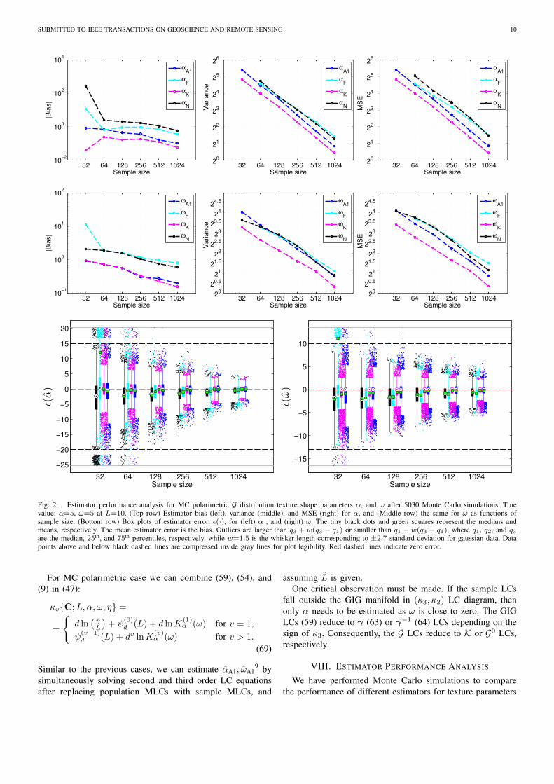
Fig. 2. Estimator performance analysis for MC polarimetric G distribution texture shape parameters α, and ω after 5030 Monte Carlo simulations. Truevalue: α=5, ω=5 at L=10. (Top row) Estimator bias (left), variance (middle), and MSE (right) for α, and (Middle row) the same for ω as functions ofsample size. (Bottom row) Box plots of estimator error, ε(·), for (left) α , and (right) ω. The tiny black dots and green squares represent the medians andmeans, respectively. The mean estimator error is the bias. Outliers are larger than q3 + w(q3 − q1) or smaller than q1 − w(q3 − q1), where q1, q2, and q3are the median, 25th, and 75th percentiles, respectively, while w=1.5 is the whisker length corresponding to ±2.7 standard deviation for gaussian data. Datapoints above and below black dashed lines are compressed inside gray lines for plot legibility. Red dashed lines indicate zero error.

For MC polarimetric case we can combine (59), (54), and(9) in (47):

κvC;L,α, ω, η =

=

d ln

(ηL

)+ ψ

(0)d (L) + d lnK

(1)α (ω) for v = 1,

ψ(v−1)d (L) + dv lnK

(v)α (ω) for v > 1.

(69)

Similar to the previous cases, we can estimate αA1, ωA19 by

simultaneously solving second and third order LC equationsafter replacing population MLCs with sample MLCs, and

assuming L is given.One critical observation must be made. If the sample LCs

fall outside the GIG manifold in (κ3, κ2) LC diagram, thenonly α needs to be estimated as ω is close to zero. The GIGLCs (59) reduce to γ (63) or γ−1 (64) LCs depending on thesign of κ3. Consequently, the G LCs reduce to K or G0 LCs,respectively.

VIII. ESTIMATOR PERFORMANCE ANALYSIS

We have performed Monte Carlo simulations to comparethe performance of different estimators for texture parameters

SUBMITTED TO IEEE TRANSACTIONS ON GEOSCIENCE AND REMOTE SENSING 11

64 128 256 512 102410

−2

100

102

104

Sample size

Bia

s

αA1

αF

αK2

αN

64 128 256 512 1024

24

26

28

210

212

214

216

218

220

222

Sample size

Va

ria

nce

αA1

αF

αK2

αN

64 128 256 512 1024

24

26

28

210

212

214

216

218

220

222

224

Sample size

MS

E

αA1

αF

αK2

αN

64 128 256 512 102410

0

101

102

103

104

Sample size

Bia

s

ωA1

ωF

ωK2

ωN

64 128 256 512 1024 2

0

25

210

215

220

225

Sample size

Va

ria

nce

ω

A1

ωF

ωK2

ωN

64 128 256 512 1024

22

24

26

28

210

212

214

216

218

220

222

Sample size

MS

E

ω

A1

ωF

ωK2

ωN

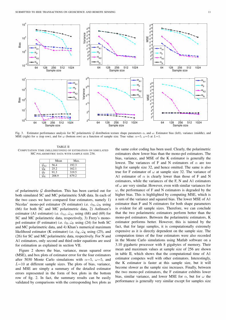
Fig. 3. Estimator performance analysis for SC polarimetric G distribution texture shape parameters α, and ω. Estimator bias (left), variance (middle), andMSE (right) for α (top row), and for ω (bottom row) as a function of sample size. True value: α=5, ω=5 at L=1.

TABLE IICOMPUTATION TIME (MILLISECONDS) OF ESTIMATION ON SIMULATED

MC POLARIMETRIC DATA WITH SAMPLE SIZE 256.

Mean Max.GA1 56.4 192.3GK 25.2 162.1GF 91.3 319.5GN 208.9 679.2

of polarimetric G distribution. This has been carried out forboth simulated SC and MC polarimetric SAR data. In each ofthe two cases we have compared four estimators, namely 1)Nicolas’ mono-pol estimator (N estimator) i.e. αN, ωN using(66) for both SC and MC polarimetric data, 2) Anfinsen’sestimator (A1 estimator) i.e. αA1, ωA1 using (68) and (69) forSC and MC polarimetric data, respectively, 3) Frery’s mono-pol estimator (F estimator) i.e. αF, ωF using (24) for both SCand MC polarimetric data, and 4) Khan’s numerical maximumlikelihood estimator (K estimator) i.e. αK, ωK using (25), and(26) for SC and MC polarimetric data, respectively. For N andA1 estimators, only second and third order equations are usedfor estimation as explained in section VII.

Figure 2 shows the bias, variance, mean squared error(MSE), and box plots of estimator error for the four estimatorsafter 5030 Monte Carlo simulations with α=5, ω=5, andL=10 at different sample sizes. The plots of bias, variance,and MSE are simply a summary of the detailed estimatorerrors represented in the form of box plots in the bottomrow of fig. 2. In fact, the summary results can be easilyvalidated by comparisons with the corresponding box plots as

the same color coding has been used. Clearly, the polarimetricestimators show lower bias than the mono-pol estimators. Thebias, variance, and MSE of the K estimator is generally thelowest. The variances of F and N estimators of α are toohigh for sample size 32, and hence omitted. The same is alsotrue for F estimator of ω at sample size 32. The variance ofA1 estimator of α is clearly lower than those of F and Nestimators, while the variances of the F, N and A1 estimatorsof ω are very similar. However, even with similar variances forω, the performance of F and N estimators is degraded by thehigher bias. This is highlighted by computing MSE, which isa sum of the variance and squared bias. The lower MSE of A1estimator than F and N estimators for both shape parametersis evident for all sample sizes. Therefore, we can concludethat the two polarimetric estimators perform better than themono-pol estimators. Between the polarimetric estimators, Kestimator performs better. However, this is tainted by thefact, that for large samples, it is computationally extremelyexpensive as it is directly dependent on the sample size. Thecomputation times of the four estimators were also recordedin the Monte Carlo simulations using Matlab software on a3.10 gigahertz processor with 8 gigabytes of memory. Theirmean and maximum values at sample size of 256 are shownin table II, which shows that the computational time of A1estimator competes well with other estimators. Interestingly,the K estimator is faster at this sample size, but it willbecome slower as the sample size increases. Finally, betweenthe two mono-pol estimators, the F estimator exhibits lowerbias, similar variance, and lower MSE for α, but for ω theperformance is generally very similar except for samples size

SUBMITTED TO IEEE TRANSACTIONS ON GEOSCIENCE AND REMOTE SENSING 12

greater than 256, where the N estimator shows lower bias,variance, and MSE. We have observed very similar bias,variance, and MSE at other values of α, ω, and L as well.

Figure 3 shows exactly the same scenario but for simulatedSC polarimetric data. The box plots have been omitted forbrevity. It should be mentioned here that, although A1 esti-mator has been derived using asymptotic statistics, we boldlyapply it on finite samples. The results clearly show that boththe polarimetric estimators perform significantly better thanthe mono-pol estimators. Between the polarimetric estimators,although A1 has a slightly higher bias than K for samplesize greater than 100, it has a significantly better variance forsample size smaller than 256. This reflects as significantlybetter MSE of A1 estimator than K estimator for samplessmaller than 256, and only slightly worse for larger samples.Keeping in perspective the computational complexity of theK estimator, we can conclude that the A1 estimator is alsoa better choice for the SC polarimetric case. Finally, overallboth the mono-pol estimators perform very poorly, with theexception of N estimator performing reasonably well only forthe ω parameter.

IX. GOODNESS OF FIT USING LOG CUMULANTS

A specialized GoF statistic, based on multiple LCs, has beenrecently developed for PolSAR distributions [31]. Tradition-ally, GoF testing has been performed by assessing the fitting ofintensity or amplitude pdfs to data histogram for each channelseparately. GoF using LCs offers a truly multivariate approach,where a single test statistic is obtained for the multivariatePolSAR data. Further, it captures more statistical informationby performing GoF using multiple LCs. In the following, webriefly list the most relevant results for the simple hypothesiscase, where the model parameters are considered known (fordetails see [31]).

Let 〈κ〉 be a p dimensional vector of sample MLCs ofselected orders v1, v2, . . . , vp:

〈κ〉 = [〈κv1〉 , 〈κv2〉 , . . . ,⟨κvp⟩]T, (70)

with mean vector κ:

E〈κ〉 = κ = [κv1 , κv2 , . . . , κvp ]T. (71)

It was shown in [31] that for sample size n:√n (〈κ〉 − κ)

D→ Np (0,K) (72)

where K is the scaled covariance matrix, given by:

K = nE

(〈κ〉 − κ) (〈κ〉 − κ)T . (73)

The mean vector κ is formed using the corresponding ppopulation MLCs of the hypothesized model, and the K matrixrequires MLCs up to order 2vmax = 2 · maxv1, v2, . . . , vp.The equation to construct K matrix using MLCs up to order2vmax is given in the appendix of [31].

We can define a test statistic, Qp, which uses p sampleMLCs:

Qp = n (〈κ〉 − κ)T

K−1 (〈κ〉 − κ) (74)

It readily follows from the multinormal assumption:

QpD→ χ2(p) (75)

where χ2(p) denotes the χ2 distribution with p degrees offreedom. Therefore, a test with a certain significance levelcan be constructed and the p value can be computed. Wehave also utilized the same theory to compute GoF for theSC polarimetric case. In this case sample MLCs are replacedby sample LCs of the FP-PWF, the rest of the theory remainsthe same.

One important remark should be made. The number ofMLCs required by GoF test is at least one more than thenumber of texture shape parameters. Thus, for the G distri-bution (two shape parameters) we utilize second, third, andfourth MLCs and, therefore require up to order eight MLCs toconstruct the K matrix. This also explains why we computedGIG LCs upto the eighth order. Finally, higher order LCs havehigher variance, therefore the relative error of order 10−4, forthe eighth GIG LC, is considered acceptable for GoF testing.

X. APPLICATION TO REAL DATA

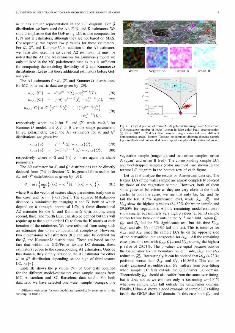
We have statistically analyzed two PolSAR images acquiredusing TerraSAR-X experimental quad-pol mode. The firstimage is over Amsterdam, which has been multilooked to have7.5 equivalent number of looks. The second one is a singlelookimage over Barcelona. Note that for both images, the resultsare organized in a way very similar to [31] for consistency,ease of comparison and clarity.

Figure 4 and 5 show the statistical analysis on Amsterdamand Barcelona images, respectively. In both cases the first rowpresents a carefully chosen subset image, which has a varietyof different types of areas. The image subsets are displayedin false color using the well known Pauli decomposition [52].From these subset images four square areas are extracted, eachof size 16 × 16 pixels. The selection process is shown astiny color-coded squares in the top row subset images. In themiddle row, the color-coded squares expand to show zoomedsample images. The sample images are selected carefullysuch that they are as homogeneous as possible so as tokeep the statistics stationary. The bottom row shows sampleLCs obtained from each extracted area and plotted using’+’ symbol in texture LC diagram. It also shows multiplecolor-coded bootstrapped sample LCs plotted for each sampleimage. These are obtained by collecting 128 bootstrap samples(using sampling with replacement [53]) each of size 128 fromthe 256-pixel sample images. We also show 95% confidenceellipses drawn using 2×2 K matrices, which are computed byutilizing sample LCs up to the fourth order10 (see [10], [31]).This gives a good idea of the statistical variation of sampleLCs for each extracted sample image.

We have also fitted K, G0, and Kummer-U distributions tothe sample images apart from the G distribution. In this way,we can compare the fitting of G distribution to the less flexibleK and G0 distributions, and also to the Kummer-U distribution

10Note that appropriate scaling by 1dv

needs to be taken into account whenconverting sample MLCs to sample texture LCs, and also in the calculationof K matrices.

SUBMITTED TO IEEE TRANSACTIONS ON GEOSCIENCE AND REMOTE SENSING 13

as it has similar representation in the LC diagram. For Gdistribution we have used the A1, F, N, and K estimators. Weshould emphasize that the GoF using LCs is also computed forF, N and K estimators, although they are not based on MKS.Consequently, we expect low p values for these estimators.For K, G0, and Kummer-U , in addition to the A1 estimator,we have also used the so called A2 estimator. It must benoted that the A1 and A2 estimators for Kummer-U model areonly utilized in the MC polarimetric case as this is sufficientfor comparing the modeling flexibility of G and Kummer-Udistributions. Let us list these additional estimators before GoFanalysis.

The A1 estimators for K, G0, and Kummer-U distributionsfor MC polarimetric data are given by [29]:

κv>1C = dvψ(v−1)(ξ) + ψ(v−1)d (L), (76)

κv>1C = (−d)vψ(v−1)(ζ) + ψ(v−1)d (L), (77)

κv>1C = dv(ψ(v−1)(ξ) + (−1)vψ(v−1)(ζ)

)+ψ

(v−1)d (L),

(78)

respectively, where v=2 for K, and G0, while v=2, 3 forKummer-U model, and ξ, ζ > 0 are the shape parameters.In SC polarimetric case, the A1 estimators for K and G0

distributions are given by:

κv>1y = ψ(v−1)(ξ) + κv>1Q, (79)

κv>1y = (−1)vψ(v−1)(ζ) + κv>1Q, (80)

respectively, where v=2 and ξ, ζ > 0 are again the shapeparameters.

The A2 estimator for K, and G0 distributions can be directlydeduced from (74) in Section IX. Its general form usable forK, and G0 distributions is given by [31]:

θ = arg

minθ

(〈κ〉 − κ)

TK−1 (〈κ〉 − κ)

, (81)

where θ is the vector of texture shape parameters (only one inthis case) and 〈κ〉 = [〈κ2〉 , 〈κ3〉]. The squared Mahalanobisdistance is minimized by changing κ and K, both of whichdepend on θ through theoretical LCs. A three dimensionalA2 estimator for the G, and Kummer-U distributions, usingsecond, third, and fourth LCs, can also be defined but this willrequire up to the eighth order LCs to form the K matrix at eachiteration of the minimizer. We have refrained from using suchan estimator due to its computational complexity. However,two dimensional A2 estimators (81) can also be defined forthe G, and Kummer-U distributions. These are based on thefact that within the GIG/Fisher texture LC domain, theseestimators reduce to the corresponding A1 estimators. Outsidethis domain, they simply reduce to the A2 estimator for eitherK or G0 distribution depending on the sign of third textureLC, κ3τ.

Table III shows the p values (%) of GoF tests obtainedfor the different model-estimators over sample images fromMC Amsterdam and SC Barcelona data sets11. For bothdata sets, we have selected one water sample (orange), one

11Different estimators for each model are symbolically represented in thesubscript in table III.

Water Vegetation Urban A Urban B

−0.1 −0.05 0 0.05

0

0.05

0.1

0.15

0.2

0.25

0.3

0.35

0.4

κ3

κ2

GIG/Fisher

γ

γ−1

δ(τ−1)

Fig. 4. (Top) A portion of TerraSAR-X polarimetric image over Amsterdam(7.5 equivalent number of looks) shown in false color Pauli decompositionc© DLR 2012 . (Middle) Four sample images extracted over different

homogeneous areas. (Bottom) Texture log cumulant diagram showing samplelog cumulants and color-coded bootstrapped samples of the extracted areas.

vegetation sample (magenta), and two urban samples, urbanA (cyan) and urban B (red). The corresponding sample LCsand bootstrapped samples (color matched) are shown in thetexture LC diagram in the bottom row of each figure.

Let us first analyze the results on Amsterdam data set. Thetexture LCs of the water sample are almost completely coveredby those of the vegetation sample. However, both of themshow gaussian behaviour as they are very close to the blackcircle. In both the cases, we see that only GF, GN, and GKfail the test at 5% significance level, while GA2, G0

A2, andUA2 show the highest p values (84.82% for water sample and89.60% for vegetation). All the remaining model-estimatorsshow smaller but similarly very high p values. Urban B sampleshows texture behaviour outside the γ−1 manifold. Again GF,GN, and GK fail the 5% significance test, but this time KA1,KA2, and also UA1 (4.73%) fail this test. This is intuitive forKA1, and KA2 since the sample LCs lie on the opposite sideof the γ manifold, but unexpected for UA1 . All the remainingcases pass this test with GA2, G0

A2, and UA2 sharing the highestp value of 20.71%. The p values are equal because outsidethe GIG/Fisher texture boundary on γ−1 side, GA2, and UA2reduce to G0

A2. Interestingly, it can be noticed that UA1 (4.73%)performs worse than GA1, and G0

A1 (16.86%). This can beeasily explained as, unlike UA2, UA1 suffers from over-fittingwhen sample LC falls outside the GIG/Fisher LC domain.Theoretically GA1 should also suffer from the same over-fitting,but it does not as we estimate only α (assuming ω=10−6)whenever sample LCs fall outside the GIG/Fisher domain.Finally, Urban A shows a good example of sample LCs fallinginside the GIG/Fisher LC domain. In this case both GA1 and

SUBMITTED TO IEEE TRANSACTIONS ON GEOSCIENCE AND REMOTE SENSING 14

Urban A Urban B Vegetation Water

−0.1 −0.05 0 0.05 0.1 0.15 0.2 0.25

−0.05

0

0.05

0.1

0.15

0.2

0.25

0.3

0.35

0.4

0.45

κ3

κ2

GIG

γ

γ−1

δ(τ−1)

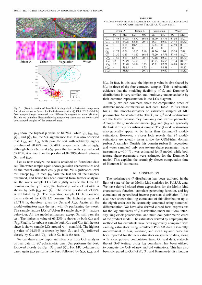
Fig. 5. (Top) A portion of TerraSAR-X singlelook polarimetric image overBarcelona shown in false color Pauli decomposition c© DLR 2012. (Middle)Four sample images extracted over different homogeneous areas. (Bottom)Texture log cumulant diagram showing sample log cumulants and color-codedbootstrapped samples of the extracted areas.

GA2 show the highest p value of 84.28%, while GF, GN, GK,G0

A1, and G0A2 fail the 5% significance test. It is also observed

that KA1, and KA2 both pass the test with relatively higherp values of 20.49% and 30.48%, respectively. Interestingly,although both UA1, and UA2 pass the test with a p value of58.85%, it is less than the p value of 84.28% shared betweenGA1 and GA2.

Let us now analyze the results obtained on Barcelona dataset. The water sample again shows gaussian characteristics andall the model-estimators easily pass the 5% significance leveltest except GN. In fact, GN fails the test for all the samplesexamined, and hence has been omitted from further analysis.As the water sample LCs fall slightly outside the GIG LCdomain on the γ−1 side, the highest p value of 94.44% isshown by both GA2 and G0

A2. The lowest p value of 73.98%is exhibited by GF. The vegetation sample LC falls outsidethe γ side of the GIG LC domain. The highest p value of85.71% is, therefore, given by GA2 and KA2. Again, all themodel-estimators pass the test, with GF performing the worst.The sample texture LCs of Urban B sample show β−1 texturebehaviour. All the model-estimators, except GF, still pass thetest. The highest p value of 63.23% is shown by both GA2 andG0

A2. Finally, for urban A sample both KA1 and KA2 fail the testsince it shows sample LCs around γ−1 manifold. The highestp value of 91.56% is shown by both GA2 and G0

A2 followedclosely by GA1 and G0

A1, while GF fails the test.We can draw a few important inferences from GoF analysis

on real data. In SC polarimetric case, GA2 performs the best,followed closely by GA1, G0

A2, and G0A1. For MC polarimetric

case, again GA2 performs the best, followed by UA2, GA1, and

TABLE IIIP VALUES (%) OVER IMAGE SAMPLES EXTRACTED FROM SC BARCELONA

AND MC AMSTERDAM TERRASAR-X DATA SETS.

Urban A Urban B Vegetation WaterSC MC SC MC SC MC SC MC

GA1 91.45 84.28 48.72 16.86 81.99 87.75 87.56 84.07GA2 91.56 84.28 63.23 20.71 85.71 89.60 94.44 84.82GF 0 0.18 0.67 0 19.44 0 73.98 0GN 0 0.09 0 0 0 0 0 0GK 91.25 0.09 10.15 2.88 84.76 1.04 93.38 2.04G0A1 91.30 0.83 41.60 16.86 73.29 87.75 87.46 84.07G0A2 91.56 3.60 63.23 20.71 79.18 89.60 94.44 84.82KA1 0.61 20.49 36.59 0.01 83.25 85.55 87.14 84.07KA2 0.61 30.48 36.59 0.23 85.71 87.27 86.89 84.82UA1 - 58.85 - 4.73 - 88.38 - 84.82UA2 - 58.85 - 20.71 - 89.60 - 84.82

UA1. In fact, in this case, the highest p value is also shared byUA2 in three of the four extracted samples. This is substantialevidence that the modeling flexibility of G, and Kummer-Udistributions is very similar, and intuitively understandable bytheir common representation in the LCs diagram.

Finally, we can comment about the computation times ofdifferent model-estimators on real data. Table IV lists thesefor all the model-estimators on extracted samples of MCpolarimetric Amsterdam data. The K, and G0 model-estimatorsare the fastest because they have only one texture parameter.Amongst the G model-estimators GA1 and GA2 are generallythe fastest except for urban A sample. The G model-estimatorsalso generally appear to be faster than Kummer-U model-estimators. However, a closer look reveals that U model-estimators are actually faster inside the GIG/Fisher domain(urban A sample). Outside this domain (urban B, vegetation,and water samples) only one texture shape parameter, i.e. α(assuming ω=10−6) , was estimated for G model, while bothtexture shape parameters were estimated for the Kummer-Umodel. This explains the seemingly slower computation timeof Kummer-U estimators.

XI. CONCLUSION

The polarimetric G distribution has been explored in thelight of state-of-the-art Mellin kind statistics for PolSAR data.We have derived closed form expressions for the Mellin kindcharacteristic function, cumulant generating function, and logcumulants of generalized inverse gaussian distribution. It hasalso been shown that log cumulants of this distribution up tothe eighth order can be accurately computed using numericaldifferentiation. We have also derived closed form expressionsfor the log cumulants of G distribution under multilook inten-sity, singlelook polarimetric, and multilook polarimetric casesof the product model. The estimators derived by employing themethod of log cumulants have been rigorously compared withexisting estimators using simulated PolSAR data. Generally,improvement in bias, variance, and mean squared error hasbeen reported for the new estimators on synthetic data, alongwith a competitive computation time. On real data, state-of-the-art GoF testing, using log cumulants, has been utilizedto compute the GoF of new and old estimators. This has alsobeen compared to GoF of K, G0, and Kummer-U distributions

SUBMITTED TO IEEE TRANSACTIONS ON GEOSCIENCE AND REMOTE SENSING 15

TABLE IVCOMPUTATION TIME (MILLISECONDS) OF ESTIMATION ON IMAGE

SAMPLES EXTRACTED FROM MC AMSTERDAM TERRASAR-X DATA.

Urban A Urban B Vegetation WaterGA1 137.5 11.3 23.8 30.4GA2 137.5 16.3 19.0 18.8GF 46.7 58.4 91.0 134.2GN 390.4 370.0 167.5 205.3GK 45.6 44.3 31.1 57.3G0A1 5.8 11.2 25.8 26.2G0A2 12.3 16.3 18.1 18.9KA1 5.7 11.3 17.0 29.8KA2 15.4 15.5 17.3 17.7UA1 8.7 106.5 87.0 53.7UA2 8.7 141.1 134.4 168.2

on real data. It can be confirmed that with the new estimators,the G distribution can not only mimic the modeling flexibilityof K, G0, and Kummer-U distributions, but can also competewell in terms of estimator computation time.

In the future, we will utilize the G distribution with its newestimators in various PolSAR image analysis algorithms likesupervised and unsupervised classification, segmentation, andtarget detection from background clutter.

ACKNOWLEDGMENT

The authors would like to extend their gratitude to StianNorman Anfinsen and Anthony Paul Doulgeris, from theUniversity of Tromsø, for their valuable comments and advice.Also, insightful comments from Alejandro Cesar Frery, fromUniversidade Federal de Alagoas, are appreciated. Finally, wewould like to thank the German Aerospace Centre (DLR) forproviding the data sets under proposal LAN0963.

REFERENCES

[1] L. Allen and D. G. C. Jones, “An analysis of the granularity of scatteredoptical maser light,” Phys. Lett., vol. 7, pp. 321–323, Dec. 1963.

[2] J. W. Goodman, “Some fundamental properties of speckle,” J. Opt. Soc.Am., vol. 66, no. 11, pp. 1145–1150, Nov. 1976.

[3] J.-S. Lee and E. Pottier, Polarimetric Radar Imaging: From Basics toApplications. Boca Raton, FL: CRC Press, Taylor & Francis Group,2009, ch. 4, pp. 101–142.

[4] C. Oliver and S. Quegan, Understanding Synthetic Aperture RadarImages, 2nd ed. Raleigh, NC: SciTech Publishing, 2004.

[5] A. Lopes, R. Garello, and S. L. Hegarat-Mascle, Processing of SyntheticAperture Radar Images. London, U.K.: John Wiley & Sons, 2008, ch. 5,pp. 87–142.

[6] A. Frery, H.-J. Muller, C. Yanasse, and S. Sant’Anna, “A model forextremely heterogeneous clutter,” IEEE Trans. Geosci. Remote Sens.,vol. 35, no. 3, pp. 648–659, May 1997.

[7] C. Tison, J.-M. Nicolas, F. Tupin, and H. Maitre, “A new statisticalmodel for Markovian classification of urban areas in high-resolutionSAR images,” IEEE Trans. Geosci. Remote Sens., vol. 42, no. 10, pp.2046–2057, Oct. 2004.

[8] C. Oliver, “Rain forest classification based on SAR texture,” IEEE Trans.Geosci. Remote Sens., vol. 38, no. 2, pp. 1095–1104, Mar 2000.

[9] T. Eltoft and K. Hogda, “Non-gaussian signal statistics in ocean SARimagery,” IEEE Trans. Geosci. Remote Sens., vol. 36, no. 2, pp. 562–575, Mar. 1998.

[10] T. Eltoft, S. Anfinsen, and A. Doulgeris, “A multitexture model formultilook polarimetric radar data,” in Proc. IGARSS, Vancouver, BC,Jul. 2011, pp. 1048–1051.

[11] S. Khan and R. Guida, “The new dual-texture G distribution for single-look PolSAR data,” in Proc. IGARSS, Munich, Germany, Jul. 2012, inpress.

[12] N. R. Goodman, “Statistical analysis based on a certain multivariatecomplex Gaussian distribution (an introduction),” Ann. Math. Statist.,vol. 34, no. 1, pp. 152–177, Mar. 1963.

[13] H. H. Lim, A. A. Swartz, H. A. Yueh, J. A. Kong, R. T. Shin, and J. J.van Zyl, “Classification of earth terrain using polarimetric SyntheticAperture Radar images,” J. Geophys. Res., vol. 94, no. B6, pp. 7049–7057, 1989.

[14] J. Lee, M. Grunes, and R. Kwok, “Classification of multi-look polari-metric SAR data based on complex Wishart distribution,” Int. J. RemoteSensing, vol. 15, no. 11, pp. 2299–2311, 1994.

[15] J.-M. Nicolas, “Introduction aux statistique de deuxieme espece: Ap-plication des logs-moments et des logs-cumulants a lanalyse des loisdimages radar,” Traitement du Signal, vol. 19, no. 3, pp. 139–167, Jun.2002, in French.

[16] ——, “Application de la transformee de mellin: Etude des lois-statistiques de lımagerie coherente,” Ecole Nationale Superieure desTelecommunications, Tech. Rep., 2006D010, in French.

[17] F. Galland, J.-M. Nicolas, H. Sportouche, M. Roche, F. Tupin, andP. Refregier, “Unsupervised synthetic aperture radar image segmentationusing Fisher distributions,” IEEE Trans. Geosci. Remote Sens., vol. 47,no. 8, pp. 2966–2972, 2009.

[18] S. Quegan, I. Rhodes, and R. Caves, “Statistical models for polarimetricSAR data,” in Proc. IGARSS, vol. 3, Pasadena, CA, Aug. 1994, pp.1371–1373.

[19] J. Lee, D. Schuler, R. Lang, and K. Ranson, “K-distribution for multi-look processed polarimetric SAR imagery,” in Proc. IGARSS, vol. 4,Pasadena, CA, Aug. 1994, pp. 2179–2181.

[20] S. H. Yueh, J. A. Kong, J. K. Jao, R. T. Shin, and L. M. Novak, “K-distribution and polarimetric terrain radar clutter,” J. Electrom. WavesAppl., vol. 3, pp. 747–768, Aug. 1989.

[21] C. Freitas, A. Frery, and A. Correia, “The polarimetric G distributionfor SAR data analysis,” Environmetrics, vol. 16, no. 1, pp. 13–31, Feb.2005.

[22] L. Bombrun and J.-M. Beaulieu, “Fisher distribution for texture mod-eling of polarimetric SAR data,” IEEE Trans. Geosci. Remote Sens.,vol. 5, no. 3, pp. 512–516, Jul. 2008.

[23] L. Bombrun, G. Vasile, M. Gay, and F. Totir, “Hierarchical segmentationof polarimetric SAR images using heterogeneous clutter models,” IEEETrans. Geosci. Remote Sens., vol. 49, no. 2, pp. 726–737, Feb. 2011.

[24] L. Bombrun, S. Anfinsen, and O. Harant, “A complete coverage of log-cumulant space in terms of distributions forpolarimetric SAR data,” inProc. PolInSAR, Frascati, Italy, 2011.

[25] S. Khan and R. Guida, “On single-look multivariate G distribution forPolSAR data,” IEEE J. Sel. Topics Appl. Earth Observations RemoteSens., vol. 5, no. 4, pp. 1149 –1163, Aug. 2012.

[26] H.-J. Muller and R. Pac, “G-statistics for scaled SAR data,” in Proc.IGARSS, vol. 2, Hamburg, Germany, Jul. 1999, pp. 1297–1299.

[27] A. C. Frery, J. Jacobo-Berlles, J. Gambini, and M. Mejail, “PolarimetricSAR image segmentation with B-splines and a new statistical model,”Multidimensional Syst. Signal Process., vol. 21, no. 4, pp. 319–342, Dec.2010.

[28] A. Doulgeris and T. Eltoft, “Scale mixture of Gaussians modelling ofpolarimetric SAR data,” EURASIP J. Adv. Signal Process, vol. 2010, no.874592, pp. 1–12, Jan. 2010.

[29] S. Anfinsen and T. Eltoft, “Application of the matrix-variate Mellintransform to analysis of polarimetric radar images,” IEEE Trans. Geosci.Remote Sens., vol. 49, no. 6, pp. 2281–2295, Jun. 2011.

[30] S. Anfinsen, “On the supremacy of logging,” in Proc. PolInSAR, Frascati,Italy, 2011.

[31] S. Anfinsen, A. Doulgeris, and T. Eltoft, “Goodness-of-fit tests formultilook polarimetric radar data based on the Mellin transform,” IEEETrans. Geosci. Remote Sens., vol. 49, no. 7, pp. 2764–2781, Jul. 2011.

[32] K. Tragl, “Polarimetric radar backscattering from reciprocal randomtargets,” IEEE Trans. Geosci. Remote Sens., vol. 28, no. 5, pp. 856–864, Sep. 1990.

[33] S. Anfinsen, “Statistical analysis of multilook polarimetric radar im-ages with Mellin transform,” Ph.D. dissertation, University of Tromsø,Tromsø, May 2010, chapter 2, Section 2.2.4.

[34] A. M. Mathai, Jacobians of Matrix Transformations and Functions ofMatrix Argument. New York: Springer-Verlag, 1997, ch. 6.

[35] L. Andrews and R. Phillips, Mathematical Techniques for Engineers andScientists. New Delhi-110001: Prentice-Hall of India, 2005, ch. 13.

[36] N. Johnson, S. Kotz, and N. Balakrishnan, Continuous UnivariateDistributions, 2nd ed. New York: John Wiley & Sons, Inc., 1994,vol. 1, ch. 15.

SUBMITTED TO IEEE TRANSACTIONS ON GEOSCIENCE AND REMOTE SENSING 16

[37] B. Jørgensen, Statistical Properties of the Generalized Inverse GaussianDistribution (Lecture Notes in Statistics). New York: World Scientific,1982, vol. 9.

[38] F. Pascal, P. Forster, J.-P. Ovarlez, and P. Larzabal, “Performanceanalysis of covariance matrix estimates in impulsive noise,” IEEE Trans.Signal Process., vol. 56, no. 6, pp. 2206–2217, Jun. 2008.

[39] F. Gini and M. Greco, “Covariance matrix estimation for CFAR detectionin correlated heavy tailed clutter,” Signal Process., vol. 82, no. 12, pp.1847–1859, Dec. 2002.

[40] A. Frery, A. Correia, and C. da Freitas, “Classifying multifrequencyfully polarimetric imagery with multiple sources of statistical evidenceand contextual information,” IEEE Trans. Geosci. Remote Sens., vol. 45,no. 10, pp. 3098–3109, Oct. 2007.

[41] A. Frery, F. Cribari-Neto, and M. Souza, “Analysis of minute featuresin speckled imagery with maximum likelihood estimation,” EURASIP J.Appl. Signal Process., vol. 2004, no. 16, pp. 2476–2491, Jan. 2004.

[42] K. L. P. Vasconcellos, A. C. Frery, and L. B. Silva, “Improvingestimation in speckled imagery,” Computational Statistics, vol. 20, no. 3,pp. 503–519, 2005.

[43] F. Cribari-Neto, A. C. Frery, and M. F. Silva, “Improved estimationof clutter properties in speckled imagery,” Computational Statistics andData Analysis, vol. 40, no. 4, pp. 801–824, 2002.

[44] L. Novak, M. Burl, and W. Irving, “Optimal polarimetric processing forenhanced target detection,” IEEE Trans. Aerosp. Electron. Syst., vol. 29,no. 1, pp. 234–244, Jan 1993.

[45] A. Stuart and J. Ord, Kendall’s Advanced Theory of Statis-tics:Distribution Theory, 6th ed. New York: John Wiley & Sons Inc.,1994, vol. 1.

[46] A. R. Hall, Generalized Method of Moments, 6th ed. Oxford, U.K.:Oxford University Press, 2005.

[47] S. Anfinsen, A. Doulgeris, and T. Eltoft, “Estimation of the equivalentnumber of looks in polarimetric synthetic aperture radar imagery,” IEEETrans. Geosci. Remote Sens., vol. 47, no. 11, pp. 3795–3809, Nov. 2009.

[48] J. Lyness and C. Moler, “Van der Monde systems and numericaldifferentiation,” Numer. Math., vol. 8, pp. 458–464, 1966.

[49] ——, “Generalized Romberg methods for integrals of derivatives,”Numer. Math., vol. 14, pp. 1–13, 1969.

[50] J. D’Errico. (2011) Adaptive robust numerical differentiation.http://www.mathworks.co.uk/matlabcentral/fileexchange/13490-adaptive-robust-numerical-differentiation. Accessed 26 Mar. 2013.

[51] ——. (2007) Derivest. http://convexoptimization.com/TOOLS/DERIVEST.pdf. Accessed 26 Mar. 2013.

[52] J.-S. Lee and E. Pottier, Polarimetric Radar Imaging: From Basics toApplications. Boca Raton, FL: CRC Press, Taylor & Francis Group,2009.

[53] B. Efron and R. Tibshirani, An Introduction to the Bootstrap, ser.Monographs on Statistics & Applied Probability. Chapman & Hall,1993, ch. 6, pp. 45–59.

Salman Khan (S’11) was born in 1982 in Lahore,Pakistan. He received B.S. degree in Computer Sci-ences from National University of Computer andEmerging Sciences, Pakistan in 2004, the M.S. de-gree in Electrical Engineering as a Fulbright scholarfrom University of Central Florida, Orlando, U.S.A.in 2009, and is currently in the fourth year ofPh.D. degree in Electronics Engineering (RemoteSensing Applications group) at the Surrey SpaceCentre, University of Surrey in Guildford, U.K. Hiscurrent research interests include Statistical Signal

Processing in polarimetric SAR, and its applications in Pattern Recognitionand Target Detection.

He is the recipient of IEEE GRSS 2013 J-STARS Prize Paper Award forthe paper titled On Single-Look Multivariate G Distribution for PolSAR Data.

Raffaella Guida (S’04–M’08) was born in Naples,Italy, on October 24, 1975. She received the Laureadegree (cum laude) in Telecommunications Engi-neering and the Ph.D. degree in Electronic andTelecommunications Engineering from the Univer-sity of Naples Federico II, Naples, in 2003 and 2007,respectively. In 2003, she received a grant from theUniversity of Naples Federico II to be spent at theDepartment of Electronic and TelecommunicationEngineering (DIET) for research in the field ofremote sensing. In 2006, she received a two-year

grant from the University of Naples Federico II to be spent at DIET forresearch in electromagnetics, particularly on the topic of electromagnetic fieldpropagation in an urban environment, within the Italian project S.Co.P.E.aimed to develop a distributed high-performance system for multidisciplinaryscientific elaborations. In 2006, she was also a Guest Scientist with theDepartment of Photogrammetry and Remote Sensing, Technische UniversittMnchen, Mnchen, Germany. In 2008, she joined the Surrey Space Centre(SSC), University of Surrey, Guildford, U.K., as Lecturer in Satellite RemoteSensing. Today she is still in SSC where she leads the Remote Sensing Appli-cations group. Her main research interests are in the fields of electromagneticsand microwave remote sensing, particularly in simulation and modeling ofsynthetic aperture radar signals relevant to natural surfaces and urban scenes,new remote sensing mission concepts and applications. She is involved as PIand co-I in many national and European research projects.