1370 IEEE TRANSACTIONS ON PATTERN ... - · PDF filePenrose Pixels for Super-Resolution Moshe Ben-Ezra, Member, IEEE, Zhouchen Lin, Senior Member, IEEE, Bennett Wilburn, Member, IEEE,

Penrose Pixels for Super-ResolutionMoshe Ben-Ezra, Member, IEEE, Zhouchen Lin, Senior Member, IEEE,

Bennett Wilburn, Member, IEEE, and Wei Zhang

Abstract—We present a novel approach to reconstruction-based super-resolution that uses aperiodic pixel tilings, such as a Penrose

tiling or a biological retina, for improved performance. To this aim, we develop a new variant of the well-known error back projection

super-resolution algorithm that makes use of the exact detector model in its back projection operator for better accuracy. Pixels in our

model can vary in shape and size, and there may be gaps between adjacent pixels. The algorithm applies equally well to periodic or

aperiodic pixel tilings. We present analysis and extensive tests using synthetic and real images to show that our approach using

aperiodic layouts substantially outperforms existing reconstruction-based algorithms for regular pixel arrays. We close with a

discussion of the feasibility of manufacturing CMOS or CCD chips with pixels arranged in Penrose tilings.

Index Terms—Super-resolution, Penrose tiling, CMOS sensor, CCD sensor.

Ç

1 INTRODUCTION

RECENT research in super-resolution (SR) has raisedsignificant concerns regarding the usability of recon-

struction-based super-resolution algorithms (RBA [7]) in thereal world. Baker and Kanade [7] showed that the conditionnumber of the linear system used in RBA and the volume ofsolutions grow quickly with increasing magnification. Linand Shum [25] showed that the effective magnification factorcan be at most 5.7. Zhao and Sawhney [35] showed that evenproperly aligning local patches for SR is difficult. More recentRBA algorithms using statistical models and image priors[34], [30], [20] are more robust and accurate, but the maximummagnification factor remains relatively low (2x to 4x).

Overcoming these limitations requires a new approach toRBA. As noted by Baker and Kanade [7], RBA can bedivided into two steps: deblurring optical blur andenhancing resolution. Multiple images taken at smallcamera displacements provide little or no additionalinformation with respect to the optical blur, so the firststep is mostly a blind image deblurring. Moreover, realoptical blur is rarely or never shift invariant (and thereforecannot be expressed by a single point spread function) andchanges with focus and aperture. This makes the problemof optical deblurring nontrivial at best.

This paper focuses on the second aspect of RBA: detectorresolution enhancement using multiple images. Opticaldeblurring can be applied to the result later, provided thatthe lens properties are known. There is a significant

technological gap, however, between the theoretical opticalresolution limits and current sensor resolutions, particularlyfor short wavelengths (380-400 �m). This is true for high-quality sensors with large pixels (9� to 15�) as well as oneswith very small pixels (2� to 4�). Moreover, sensortechnology advances more slowly than may be expected[12], while physics is already exploring the feasibility of a“perfect lens” using materials with negative indexes ofrefraction [29]. Therefore, there is a clear need for resolutionenhancement at the sensor level.

1.1 Related Work

Roughly speaking, SR algorithms can be categorized intofour classes [11], [27], [15]. Interpolation-based algorithmsregister low-resolution images (LRIs) with the high-resolu-tion image (HRI), then apply nonuniform interpolation toproduce an improved-resolution image, which is thendeblurred. Frequency-based algorithms try to de-alias theLRIs using the phase differences between the LRIs.Learning-based algorithms (e.g., [17], [7]) incorporateapplication-dependent priors to infer the unknown HRI.Reconstruction-based algorithms rely on the relationshipbetween the LRIs and the HRI and assume various kinds ofpriors on the HRI in order to regularize this ill-posedinverse problem. Among these four categories of algo-rithms, RBAs are the most commonly used SR algorithms.RBAs usually first form a linear system

L ¼ PH þ E; ð1Þ

where L is the column vector of the irradiances of all thelow-resolution pixels (LRPs), H is the vector of theirradiances of the HRI, P gives the weights of the high-resolution pixels (HRPs) in order to obtain the irradiance ofthe corresponding LRPs, and E is the noise. Past methods tosolve (1) for the HRI include maximum a posteriori (MAP)[21], [14], regularized maximum likelihood (ML) [14],projection onto convex sets (POCS) [28], and iterative backprojection [23].

In all previous work, the LRPs appear on the left handside of the system (1) and the LRI pixel layouts are allregular grids, with square pixels. Based on such a

1370 IEEE TRANSACTIONS ON PATTERN ANALYSIS AND MACHINE INTELLIGENCE, VOL. 33, NO. 7, JULY 2011

. M. Ben-Ezra and Z. Lin are with Microsoft Research Asia, 5F, BeijingSigma Center, 49 Zhichun road, Haidian district, Beijing 100190, China.E-mail: {mosheb, zhoulin}@microsoft.com.

. B. Wilburn is with Refocus Imaging, 10607 Vickers Dr., Vienna,VA 22181. E-mail: [email protected].

. W. Zhang is with the Department of Information Engineering, The ChineseUniversity of Hong Kong, Room 703, Ho Sin Hang Engineering Building,The Chinese University of Hong Kong. E-mail: [email protected].

Manuscript received 16 July 2009; revised 28 July 2010; accepted 22 Oct.2010; published online 29 Nov. 2010.Recommended for acceptance by D. Forsyth.For information on obtaining reprints of this article, please send e-mail to:[email protected], and reference IEEECS Log NumberTPAMI-2009-07-0456.Digital Object Identifier no. 10.1109/TPAMI.2010.213.

0162-8828/11/$26.00 � 2011 IEEE Published by the IEEE Computer Society

configuration, both the practical and theoretical analyses[7], [25] have shown that the magnification factor is limitedto a relatively small number.

Nonrectangular pixel layouts, mostly hexagonal, havebeen studied [1] for a range of imaging tasks, such as edgedetection [26]. Nonrectangular layouts have also been usedto increase pixel density, as in the new Fujifilm super CCD.However, these sensors all use periodic tiling and sufferfrom the same limitations as rectangular tiling with respectto super-resolution. Random sampling was used in thecontext of compressive sensing [33], [16]. Although Penrosetiling is quasi-random, the compressive sensing frameworkis very different because RBA is not compressive, andrandom sampling (tiling) is not considered an aperiodictiling since the set of tiles is not finite.

1.2 Our Contributions

We increase the RBA magnification factor by breaking thetwo aforementioned conventions. Rather than using aregular pixel grid for the LRIs, we use aperiodic layouts forthe detector, resulting in LRIs with an irregular pixel layout.The irregular layout leads to a much more independentequation set. Most importantly, since our layout has notranslational symmetry, we can use larger displacements(multiples of half a pixel) between LRIs without having thegrid repeat itself. This enables computation of the HRI withlarger magnifications. For regular grids, by contrast, theeffective displacement is modulo pixel size, which limits thenumber of different displacements that are at least � apart.We argue that manufacturing a Penrose pixel image sensoris feasible given current technologies and also discuss thepotential benefits of such sensors that are not directlyrelated to super-resolution.

To recover a high-resolution image from the raw datacaptured by the aperiodic pixel layouts, we propose avariant of the traditional error back projection algorithm.Rather than using the LRPs directly for the left-hand side of(1), we upsample the LRIs to the high-resolution grid tomatch the detector’s actual layout (for example, nonsquarepixels with small gaps between them), as shown in Figs. 1aand 1d. For a perfectly square pixel layout, this is identicalto a nearest neighbor interpolation. In theory, this isequivalent to multiplying a matrix involving the upsam-pling to both sides of (1). This treatment results in verydifferent behavior in the presence of noise. This isanalogous to preconditioning techniques [18] for solvinglinear systems. Our model does not require that the LRPsfill the whole detector plane, for either regular or irregularlayouts. We specifically model the gaps between physicalpixels as null values, which better matches the informationthat is actually acquired by the sensor. Our novel error backprojection algorithm iteratively recovers the super-resolvedimage for arbitrary pixel layouts, either regular or irregular.

2 OPTICS AND DETECTOR PROPERTIES

Super-resolution has been addressed mostly from a compu-tational point of view, focusing on the conditioning of thereconstruction problem with respect to noise and quantiza-tion errors [7], [25]. Little attention is paid to the blurfunctions of real lenses and the sampling properties of realsensors. These are often approximated by a Gaussian blur forthe lens and a box function for the sensor. In this section, we

discuss lens blur and spatial integration, and their impact onthe performance of super-resolution of real images.

2.1 Modulation Transfer Function andSuper-Resolution

The modulation transfer function MTF ð Þ of a lens systemdescribes how sharp a spatial sine wave will appear on theimage plane prior to being sampled by the sensor. The MTFdrops as the spatial frequency increases and limitsthe achievable magnification factor for super-resolution.To see this, consider a 1D case in which a perfect ½0; 1�vertical edge passes through a pixel. For a quantizationlevel of � and a pixel size of 1, the minimum displacementthat produces a detectable change (above the quantizationlevel) in the measured pixel intensity would be dmin ¼ �.This implies that 1

� different values are obtained as the edgemoves across the pixel. If the contrast level drops to½0:25; 0:75�, however, then the minimum detectable displa-cement would be dmin ¼ 2�, thereby halving the number ofpossible different values.

For periodic tiling such as square pixel tiling, themaximum displacement before the complete image repeatsis the tiling period length (one pixel for square pixel tiling).To collect more images, one must use shorter and shorterdisplacements. As the contrast level drops, however, smalldisplacements will cause fewer and fewer pixels to changevalue (above noise level and quantization error). This is afundamental limit for super-resolution using periodic tiling.By contrast, one can collect many measurements withaperiodic tilings using a series of half-pixel displacementsin any given direction. Later, we will show that this leads toa much better conditioned system of equations for super-resolution.

2.2 Modeling Real Lens Blur

The MTFs of real lenses vary with distance from the opticalcenter, orientation, focus, and of course aperture changes.Figs. 2a and 2b show the measured MTF of a Carl Zeiss

BEN-EZRA ET AL.: PENROSE PIXELS FOR SUPER-RESOLUTION 1371

Fig. 1. A regular pixel layout and a Penrose pixel layout on the detectorplane. (a) A microscopic view of a Sony 1=300 sensor (part). Our methodmodels the nonsquare shape of the pixels as well as the gaps betweenthem. (b) A hypothetical aperiodic Penrose pixel layout. (c) An exampleimage at the sensor surface (irradiance). (d) Spatial integration for theconventional layout. (e) Spatial integration for the Penrose layout.

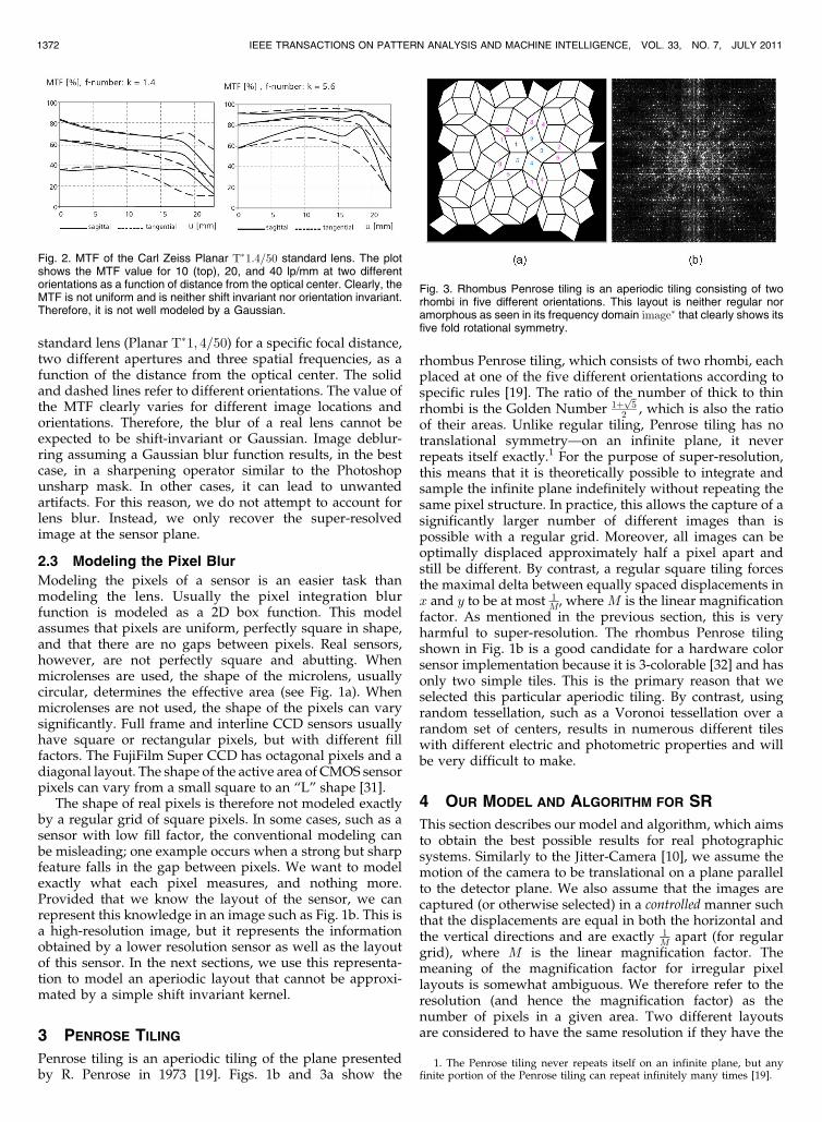
standard lens (Planar T�1; 4=50) for a specific focal distance,two different apertures and three spatial frequencies, as afunction of the distance from the optical center. The solidand dashed lines refer to different orientations. The value ofthe MTF clearly varies for different image locations andorientations. Therefore, the blur of a real lens cannot beexpected to be shift-invariant or Gaussian. Image deblur-ring assuming a Gaussian blur function results, in the bestcase, in a sharpening operator similar to the Photoshopunsharp mask. In other cases, it can lead to unwantedartifacts. For this reason, we do not attempt to account forlens blur. Instead, we only recover the super-resolvedimage at the sensor plane.

2.3 Modeling the Pixel Blur

Modeling the pixels of a sensor is an easier task thanmodeling the lens. Usually the pixel integration blurfunction is modeled as a 2D box function. This modelassumes that pixels are uniform, perfectly square in shape,and that there are no gaps between pixels. Real sensors,however, are not perfectly square and abutting. Whenmicrolenses are used, the shape of the microlens, usuallycircular, determines the effective area (see Fig. 1a). Whenmicrolenses are not used, the shape of the pixels can varysignificantly. Full frame and interline CCD sensors usuallyhave square or rectangular pixels, but with different fillfactors. The FujiFilm Super CCD has octagonal pixels and adiagonal layout. The shape of the active area of CMOS sensorpixels can vary from a small square to an “L” shape [31].

The shape of real pixels is therefore not modeled exactlyby a regular grid of square pixels. In some cases, such as asensor with low fill factor, the conventional modeling canbe misleading; one example occurs when a strong but sharpfeature falls in the gap between pixels. We want to modelexactly what each pixel measures, and nothing more.Provided that we know the layout of the sensor, we canrepresent this knowledge in an image such as Fig. 1b. This isa high-resolution image, but it represents the informationobtained by a lower resolution sensor as well as the layoutof this sensor. In the next sections, we use this representa-tion to model an aperiodic layout that cannot be approxi-mated by a simple shift invariant kernel.

3 PENROSE TILING

Penrose tiling is an aperiodic tiling of the plane presentedby R. Penrose in 1973 [19]. Figs. 1b and 3a show the

rhombus Penrose tiling, which consists of two rhombi, eachplaced at one of the five different orientations according tospecific rules [19]. The ratio of the number of thick to thinrhombi is the Golden Number 1þ

ffiffi5p

2 , which is also the ratioof their areas. Unlike regular tiling, Penrose tiling has notranslational symmetry—on an infinite plane, it neverrepeats itself exactly.1 For the purpose of super-resolution,this means that it is theoretically possible to integrate andsample the infinite plane indefinitely without repeating thesame pixel structure. In practice, this allows the capture of asignificantly larger number of different images than ispossible with a regular grid. Moreover, all images can beoptimally displaced approximately half a pixel apart andstill be different. By contrast, a regular square tiling forcesthe maximal delta between equally spaced displacements inx and y to be at most 1

M, where M is the linear magnificationfactor. As mentioned in the previous section, this is veryharmful to super-resolution. The rhombus Penrose tilingshown in Fig. 1b is a good candidate for a hardware colorsensor implementation because it is 3-colorable [32] and hasonly two simple tiles. This is the primary reason that weselected this particular aperiodic tiling. By contrast, usingrandom tessellation, such as a Voronoi tessellation over arandom set of centers, results in numerous different tileswith different electric and photometric properties and willbe very difficult to make.

4 OUR MODEL AND ALGORITHM FOR SR

This section describes our model and algorithm, which aimsto obtain the best possible results for real photographicsystems. Similarly to the Jitter-Camera [10], we assume themotion of the camera to be translational on a plane parallelto the detector plane. We also assume that the images arecaptured (or otherwise selected) in a controlled manner suchthat the displacements are equal in both the horizontal andthe vertical directions and are exactly 1

M apart (for regulargrid), where M is the linear magnification factor. Themeaning of the magnification factor for irregular pixellayouts is somewhat ambiguous. We therefore refer to theresolution (and hence the magnification factor) as thenumber of pixels in a given area. Two different layoutsare considered to have the same resolution if they have the


Fig. 2. MTF of the Carl Zeiss Planar T�1:4=50 standard lens. The plotshows the MTF value for 10 (top), 20, and 40 lp/mm at two differentorientations as a function of distance from the optical center. Clearly, theMTF is not uniform and is neither shift invariant nor orientation invariant.Therefore, it is not well modeled by a Gaussian.

1. The Penrose tiling never repeats itself on an infinite plane, but anyfinite portion of the Penrose tiling can repeat infinitely many times [19].

Fig. 3. Rhombus Penrose tiling is an aperiodic tiling consisting of tworhombi in five different orientations. This layout is neither regular noramorphous as seen in its frequency domain image� that clearly shows itsfive fold rotational symmetry.

same number of pixels within a given area (up to arounding error).

The shape of LRPs can also be different from each other,and gaps between pixels are allowed. As in [8], [7], [25], wealso assume that the pixels of the sensor have uniformphotosensitivity, which implies that the contribution of anHRP to an LRP is proportional to its area inside the LRP andvice versa. These assumptions greatly simplify our modeland implementation, but, as we show later in this section,they can easily be relaxed.

4.1 Upsampling and Resampling

In our approach, the LRPs in each LRI may not be aligned ona regular grid. Nonetheless, we can still index each LRP in anLRI because we have full knowledge of the pixel layout. Assoon as an LRI is captured, we immediately upsample it tothe high-resolution grid to create an intermediate HRI. Thisintermediate HRI, not the original LRI, is involved in thecomputations that follow. As shown in Fig. 4, upsampling isdone by placing a regular high-resolution pixel grid over theactual shape of the low-resolution pixels and then mappingHRPs to LRPs. HRPs that are not associated with any LRP areassigned the value null to differentiate them from the valuezero. The assumption of pixel uniformity can be relaxed atthis stage by multiplying the intermediate HRI with a weightmask to compensate for any intrapixel nonuniformities. Forfronto-parallel translational motion with image displace-ments equal to 1

M, it turns out that the registration of theintermediate HRI is simply an integer shift of the origin. Ifthe motion assumptions do not hold, an additional warpingstep is required after the upsampling. We denote theupsampling operator by "Ti;G , where Ti is the transformationfor registration and G is the sensor layout map.

Our algorithm also includes an error back projectionprocedure. It requires a resampling operator (Fig. 4),denoted by lTi;G , which simulates the image formationprocess to produce new intermediate HRIs given anestimate of the super-resolved image. The resamplingoperator can be viewed as a downsampling operatorfollowed by an upsampling operator. An alternative wayto view the upsampling and resampling operators is to viewthe downsampling operator as filling each LRP with theaverage value of the HRPs inside it, and the upsampling/resampling operator as filling the HRPs inside the same LRPwith their average value. In practice, the computation isdone “in-place” and no actual downsizing takes place. The

resulting images are hypotheses of the intermediate HRIs,assuming that the super-resolved image is the correct one.

4.2 Error Back Projection Algorithm

Our super-resolution algorithm is a variant of the well-known error back projection super-resolution algorithm[23]. Unlike the traditional algorithm, which downsamplesthe images into a low resolution array, our algorithm isperformed entirely on the high-resolution grid. Using theconcepts in the previous section, we summarize ouralgorithm as follows:

Algorithm 1

Inputs:

. L1; . . . ; LM2 : Low resolution images (with roughly

N2 pixels).

. T1; . . . ; TM2 : Transformations for registering the LRIs.

. M 2 N : Magnification factor.

. G: Sensor layout map.

Output:

. S: Super-Resolved image ðNM �NMÞ.Processing:

1) Upsample: Hi ¼ Li "Ti;G; i 2 ½1; . . . ;M2�.

2) Initialize: S0 ¼ 1

M2

XM2

i¼1

Hi.

3) Iterate until convergence:

a. Skþ1 ¼ Sk þ 1

M2

XM2

i¼1

ðHi � Sk lTi;GÞ.

b. Limit: 0 � Skðx; yÞ � MaxVal.

Note that null elements are ignored when computing theaverage values. Step 3)b represents the prior knowledgeabout a physically plausible image, where MaxVal isdetermined by the optical blur and the A/D unit. Thedifference between our algorithm and the conventionalback projection algorithm (with a rect kernel) lies in theupsample stage. Our upsampling operator "T;G preservessharp edges between pixels at the high-resolution grid,whereas the conventional algorithm applies the blur kernelglobally. If warping is required, it is performed on theintermediate HRI after the upsampling.

5 ANALYSIS

In this section, we analyze our super-resolution algorithm(Algorithm 1) and the irregular Penrose pixel layout. Webegin by analyzing the error bounds for our algorithm andshowing that it converges more closely to the ground truthfor an appropriately chosen aperiodic pixel layout than for aperiodic one. We also discuss the condition number of theRBA system of equations and show that the Penrose pixeltiling leads to a better conditioned system, which is thusmore robust to noise. Finally, we look at the informationcontent of Penrose Pixel and regular pixel layout LRIs andpresent experimental results suggesting that sets of PenrosePixel LRIs contain more information.

5.1 Convergence of the Algorithm

For the jth LRP of the ith LRI, its downsampling and

upsampling operators can be represented by N�1j ðpijÞ

T and


Fig. 4. Upsampling and resampling. Upsampling is done by placing aregular high-resolution pixel (HRP) grid over the actual shape of the lowresolution pixels (LRP), shown as white areas, then assigning the valueof the LRP to each of the HRPs covering it. HRPs that (mostly) coverblack areas (non-photo-sensitive areas) are assigned the value null.Downsampling is an inverse procedure that integrates the nonnull HRPvalues to form the value of its underlying LRP. Resampling is thecomposition of downsampling and upsampling.

pij, respectively, where Nj is the number of HRPs inside the

jth LRP and pij is a binary vector: pijðkÞ ¼ 1 indicates that the

kth HRP is inside the jth LRP of the ith LRI, and pijðkÞ ¼ 0 if

not. The superscript T denotes transpose. Then the resam-

pling operator, as the composition of downsampling and

upsampling, associated with the jth LRP of the ith LRI is

N�1j pijðpijÞ

T . Hence, the resampling matrix representing the

resampling operator lTi;G in Algorithm 1 can be written as

Ri ¼Xj

N�1j pijðpijÞ

T : ð2Þ

So, every intermediate HRI Hi aligned to the high-

resolution grid is connected to the ground truth image S

via the following linear system:

Hi ¼ Ri � S þ ni; i ¼ 1; 2; . . . ;M2; ð3Þ

where ni are the noise from Li. As the pixel shape and

layout of LRPs is irregular, it is difficult to write down

exactly how Ri looks. Also, as mentioned in the previous

section, in practice we do not explicitly compute the down/

up resampling matrices.The iteration 3)a in Algorithm 1 can be written as

Skþ1 ¼ Sk þ 1

M2

XM2

i¼1

Ri � S þ ni �Ri � Sk� �

; ð4Þ

which can be rewritten as

Skþ1 � S ¼ ðI � �RÞðSk � SÞ þ �n; ð5Þ

where �R ¼ 1M2

PM2

i¼1 Ri and �n ¼ 1M2

PM2

i¼1 ni. So,

Sk � S ¼ ðI � �RÞkðS0 � SÞ þXk�1

j¼0

ðI � �RÞj" #

�n: ð6Þ

We can prove that the spectral radius of I � �R is usually

less than one (see the Appendix), then limk!1ðI � �RÞk ¼ 0

and �R is nonsingular with �R�1 ¼P1

j¼0ðI � �RÞj. Then, from

(6), we have that

limk!1

Sk ¼ S þ �R�1 �n; ð7Þ

which means that iteration 3)a in Algorithm 1 converges toan HRI which deviates from the ground truth by �R�1 �n.

5.2 Error Analysis and Numerical Stability

From (7), we may expect that the iterations result in a super-resolved image which deviates from the ground truth by�R�1 �n. Note that �n can be viewed as the empirical estimationof the mean of the noise. Therefore, when the noise in theLRIs is of zero mean (and so is ni, as there is a lineartransform between them), we can expect that a high-fidelitysuper-resolved image is computed. If we choose anappropriate pixel layout so that the norm of �R�1 is small,then the deviation can be effectively controlled regardless ofthe mean of the noise (note that k limk!1 S

k � Sk ¼k �R�1 �nk � k �R�1kk�nk). As k �R�1k is large when �R is close tosingular, we should choose an appropriate detector pixellayout such that �R is far from singular.

According to the above analysis, we should choose pixellayouts that result in more linearly independent equationsin the system (3). The traditional regular tiling repeats itselfafter a translation of one LRP (two LRPs if we account forthe Bayer pattern in color sensors). Lin and Shum [25] alsoshowed that if five LRPs cover the same set of HRPs, thentheir equation set must be linearly dependent. Thus, usingregular (and square) tilings usually results in an insufficientnumber of independent equations. To overcome thisdifficulty, we try to change the regular tiling to other kindsof tilings. An intuition is to use aperiodic tilings.

In an attempt to quantify the difference between thePenrose LRIs and the regular LRIs, we empiricallycomputed the condition number as well as the numericalrank (the number of singular values larger than a threshold)of P from (1) for different magnification factors. Figs. 5a, 5b,and 5c show the condition numbers and the numericalranks with respect to different thresholds for Penrose pixelsand periodic square pixels as a function of the magnifica-tion factor. We can see for the same magnification factor, thecondition numbers for the Penrose layout are up to an orderof magnitude lower than those for the square pixels, and thenumerical ranks for the Penrose layout are larger than thosefor the square pixels. We can also see that the conditionnumber for the Penrose layout is much more stable than


Fig. 5. Comparison of (a) the condition number and (b) the numerical rank for Penrose pixel and square pixel layouts. Fixed threshold (0.05) anddifferent magnification factors. (c) Numerical rank for the Penrose pixel and square pixel layouts. Fixed magnification factor (�8) and differentthresholds. The Perose layout is more numerically stable with respect to both the condition number and the numerical rank.

that for the square pixels in that it does not suffer fromnumerical instability at integer magnification factors [7],[25]. The numerical rank is similar. These plots show thatthe linear system for the Penrose layout is much more stablethan that for the regular square layout.

5.3 Improved Conditioning Using the ResamplingOperator

The previous section presented empirical evidence of thesuperior conditioning of Penrose Pixel RBA. We nowexplain why the resampling operator can result in betterSR performance than traditional reconstruction-basedmethods. Equation (3) leads to the following overdeter-mined linear system:

H ¼ R � S þ n; ð8Þ

where H ¼ ðHT1 ; H

T2 ; . . . ; HT

M2ÞT , R ¼ ðRT1 ; R

T2 ; . . . ; RT

M2ÞT ,and n ¼ ðnT1 ; nT2 ; . . . ; nTM2ÞT . By contrast, the traditionalformulation for reconstruction-based SR is

Li ¼ Di � S þ ei; i ¼ 1; 2; . . . ;M2: ð9Þ

Here, ei is the noise from Li and the matrix Di is therepresentation of the downsampling operator in Fig. 4,leading to the following overdetermined linear system:

L ¼ D � S þ e; ð10Þ

where L ¼ ðLT1 ; LT2 ; . . . ; LTM2ÞT ,D ¼ ðDT1 ; D

T2 ; . . . ; DT

M2ÞT , ande ¼ ðeT1 ; eT2 ; . . . ; eTM2ÞT . The major difference between (3) and(9) is that Di is roughly a submatrix of Ri (Ri has manymore rows than Di). So, D is also roughly a submatrix of R.It is well known in matrix theory [22] that, in this case, theminimum singular value of R, defined by �minðRÞ ¼minx 6¼0 kRxk=kxk, will be no smaller than that of D. Thisincrease of the minimum singular value can greatly reducethe condition number of the corresponding linear system,particularly when the original system (10) is ill-conditioned.Although the maximum singular value of R is also largerthan that of D, our numerical simulation shows that withvery high probability, the condition number, defined as theratio of the maximum singular value to the minimum one,is reduced by adding rows to a matrix. When the originalmatrix is very well conditioned, it happens occasionally thatthe condition number increases slightly, so the robustness ofthe system is virtually unchanged. Generally speaking,using the resampling operator instead of the traditionaldownsampling operator can result in a much betterconditioned system. As a consequence, better SR resultsare possible.

5.4 Information Content for Penrose Pixel LRI’s

Intuition suggests that because Penrose pixel views can allbe displaced by half LRP intervals, the differences betweenadjacent views would be larger than for regular pixels,which must be displaced by 1

M (M > 2). When subject toquantization error, this should provide an advantage to thePenrose pixels over the regular one. How can we verify thisquantitatively? Here, we present a rough empirical estimateof the relative information content of regular and Penrosepixel layouts. We do this using gzip to compress imagescaptured using both layouts. Gzip uses LZ77, which forlarge file sizes converges to optimal compression.

We assume that, for real images (in contrast to specialcases like pseudo-random data), lossless compression ismonotonic, i.e., a larger compressed file implies larger datacomplexity. We assume neither optimality nor linearity of thecomplexity with respect to the file size. We also ignore thelayout description of both the Penrose and regular pixel tilingbecause Penrose and regular tillings of the infinite plane canbe described by a finite (and relatively small) set of rules.Because the layouts do not match, it is not clear in whichorder to serialize the pixels, as this may introduce a bias. Wesolve this problem by using the nonoptimal, but nonbiased,LRI representation in the high-resolution grid and simplycompressing the views in the high-resolution grid.

For our comparison we used the regular and Penroselayouts shown in Figs. 1d and 1e. Both are nonsquare pixels,both have gaps between pixels, and both have the sameaverage area. We did the following:

1. Create 64 images for �8 magnification factor forPenrose and regular pixel layouts. The displacementstep is 1

8 pixel for the regular tiling and 12 pixel for the

Penrose tiling.2. Concatenate all views into a single file to allow the

compression algorithm to apply dictionary entriesobtained in one view to other views.

3. Compress the concatenated file using gzip andrecord the absolute file size.

4. Repeat steps 1-3 for quantization levels of 8, 6, 4, and2 bits.

5. Repeat steps 1-4 for magnification factor of 16x, and256 images.

Fig. 6 displays the compressed file size (in K-bytes) fordifferent quantization levels and magnification factors. Thefirst thing to notice is that although the number of imagesfor the magnification factor of 16x was four times largerthan those for 8x magnification, the compressed file size isvery similar, even slightly smaller. This indicates that theamount of information in these sets did not changesignificantly (slight variations are expected due to conver-gence properties of the algorithm and technical reasons


Fig. 6. File sizes of sample (low resolution) image sets for Penrose andregular tiling compressed by gzip. The compressed size of the Penrosetiling set is consistently larger than the size of the compressed regularset. The compressed size of �8 (64 images) and �16 (256 images) forthe same quantization level is very similar. This indicates (but does notprove) that the Penrose tiling possesses more information than theregular tiling for the same number of pixels.

such as the dictionary size). We also see that the Penrosetiling LRIs are consistently and quite significantly com-pressed to a larger file size than the regular tiling LRIs, andthat the difference grows with the quantization level. Thissuggests that the Penrose tiling LRIs do contain moreinformation than the regular ones. This is due to thecombined effect of the displacement size, the pixel aper-iodicity, and the existence of two different pixel shapes.

6 TESTING AND EVALUATION

We evaluated our approach with simulations and realimage tests. For our first experiment, we simulated theentire super-resolution process for square and Penrosepixels. The integration of each pixel was approximatedusing the sum of the pixels in the high-resolution grid thatare enclosed within the low-resolution grid pixel area. Aswe do not have an actual Penrose pixel sensor, our secondexperiment strives to be as close to real world conditions aspossible. We first captured a sequence of high-resolutionreal images (each with its own unique noise values) andthen integrated pixel values to simulate a Penrose image.The last experiment is a start-to-finish real image super-resolution test.

To fully utilize the advantage of the aperiodic layout,and to overcome noise, we usually used more images thanunknowns. The advantage of using an overdeterminedsystem is shown in Fig. 12. For the case of square pixels andquantization error only, we used M2 input images, whereM is the magnification factor. This is the maximum numberof different images we can obtain using a displacement of 1

M.The number of input images used in each test appears in thecaptions of the relevant figures.

6.1 Regular Pixels Quantization and Noise Tests

In our first simulation, we applied our algorithm to LRIssynthesized from ground truth HRIs of a clock and a face.

We used regular grids with linear magnification factors of 1to 16, and quantization levels of 8 and 5 bits. No additionalnoise was added. Fig. 7 shows our super-resolution resultsand RMS errors (compared to the original image). Thoughthere is a gradual degradation with increasing magnifica-tion and quantization error, the super-resolution algorithmperforms very well. This matches our analysis for zeromean (quantization) noise.

Next, we added Poisson noise (which better models realnoise) to the input images. Fig. 8 shows the super-resolutionresult for the “face” image using additive Poisson noisewith mean = 5 and 10 gray levels, followed by 8-bitquantization. Unlike the zero-mean quantization error, thenonzero mean Poisson noise significantly degrades thequality of the results. The results can be improved by usingmany more images than the theoretical minimum require-ment, as shown in the bottom row of Fig. 8.

6.2 Penrose Pixels Quantization and Noise Tests

We repeated the last two tests for two Penrose tiling pixellayouts. The magnification factors were roughly equivalentto 8 and 16, and the quantization level was 8-bit. Unlike forregular pixels, we used displacements of approximately0.5 pixels and were able to use more images than waspossible with the regular grid. The results shown in Fig. 9are clearly better than the results obtained with the regulargrid, shown in Figs. 7 and 8.

To better quantify the results, we used a concentric testtarget having variable spatial frequency contrast.2 We addedlow-level noise to each image to create quantization varia-tions. Then, we applied our algorithm and the conventionalback projection algorithm under exactly the same conditionsand using the same number of input images. Fig. 10 showsthat our algorithm improves the linear magnification by


Fig. 7. Effects of Quantization Error: Super-resolution results for the “clock” and “face” images using regular tiling. Top left corner: Original image.Top row: LRIs with different magnification factors (scaled). Center and bottom rows: Super-resolution results for quantization levels of 8 and 5 bits,respectively. The results gradually degrade as the quantization error and magnification increase. Parentheses are the RMS errors. M2 input imageswere used.

2. The contrast of real lenses decreases as the spatial frequency increases.

roughly a factor of two (for the same RMS errors) compared tothe conventional back projection algorithm with regularpixels, and by over a factor of four when Penrose pixels arealso used. In this test, we also compared to the RMS errors ofthe conventional algorithm with a noninteger magnificationfactor to rule out the possibility that the difference is due tothe integer magnification used in our algorithm [7]. Asshown in Fig. 10 the integer magnification factor did notaffect the results for the back projection algorithm.

Fig. 12 compares the RMS error as a function of thenumber of images for regular and Penrose tiling, respec-tively. The magnification factor was eight and the samealgorithm (Algorithm 1) was applied to both layouts. Whilethe regular layout improved slightly when overconstrained,the Penrose layout improved by over four times. It isinteresting to see that the regular layout was actually betterwhen the system was severely underconstrained.

Fig. 13 shows different image types and the conver-gence of the algorithm (RMS error) as a function of thenumber of iterations.

For our last simulation example, we compared ouralgorithm to an externally obtained result of [21], [7] usingan image from the FERET database [6]. In Fig. 11, theimprovement from our approach is clearly visible.

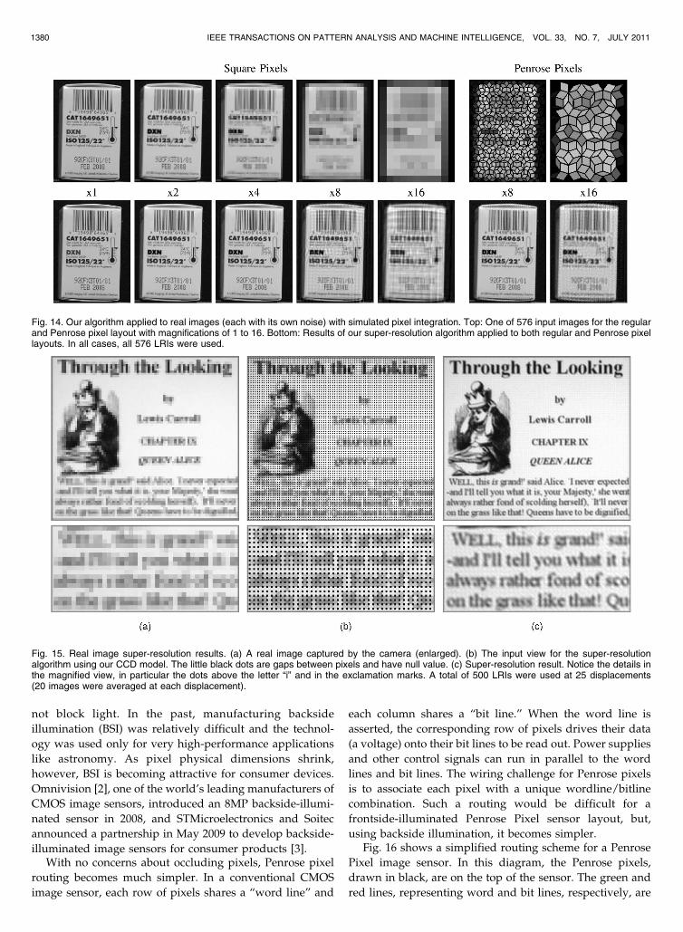
6.3 Real Images with Simulated Binning Test

In this test, we captured 576 real images with a Nikon D70camera on a tripod. We computed the LRIs by integratingeach image with the map G, then quantizing the result.Thus, the resulting LRIs had unique noise due to sensornoise, quantization, and JPEG compression. This process is

very similar (though noisier) to pixel binning done at the

analog level. As with pixel binning in real sensors, large

simulated pixels have lower noise than small integrated

pixels do. The LRIs were also subject to slight misalignment

due to shake by the flipping mirror in the camera.

Capturing more images than the required minimum

reduces the effect of slight misalignments. Fig. 14 shows

the results of applying our super-resolution algorithm to the

LRIs for regular and Penrose layouts. The advantage of the

Penrose layout is clear.

6.4 Real Scenario Test

For our real-world test, we captured a sequence of images

using a B/W version of the Sony 1=300 sensor shown in

Fig. 1a. Using the lens resolution and pixel size and shape,

we created a sensor model for �5 magnification (which is

above the nominal lens resolution). We model square pixels

with trimmed (null) corners to match the actual pixel shape,

including the microlens. We then moved a test image, in a

controlled manner, in front of the camera and captured 5� 5

input images at 25 different displacements. To reduce noise,

we averaged 20 frames for each input image.3 Fig. 15a shows

one of the input images and a magnified insert. Fig. 15b

shows an actual intermediate HRI. The black dots are the

null values at the corners of each pixel. Fig. 15c shows the

super-resolution result. Note that even fine details such as

the dots above the letter “i” and in the exclamation marks

were resolved.


Fig. 9. Penrose Pixel super-resolution results. (Top) Input images formagnification factors of 8 and 16. (Middle) 8-bit quantization result.Compare to the corresponding images in Fig. 7. (Bottom) 8-bitquantization, and Poisson noise results. Compare the image labeled“� 10�8 625” to its corresponding image in Fig. 8. The overconstraintnumber of different LRIs used was 625 for �8 and 1,600 for �16 in allcases.

Fig. 8. Noise evaluation test using regular tiling. The top two rows showthe results of super-resolution with different magnification factors andPoisson noise of mean 5 (top) and 10 (middle) gray levels. M2 LRIswere used and all computations were run for several thousand iterationsor until convergence. The amplification of noise is quite clear and theresults are very different from those with zero-mean quantization errorshown in Fig. 7. The bottom row shows the results of super-resolutionwith magnification of �8 and noise mean of 10 running for 1,000iterations, with different numbers of input images (256 to 1,600). Theresults are much better than that obtained by using the minimum64 input images (the boxed image).

3. This is possible in a controlled environment such as the “JitterCamera” [10], and saves a lot of storage space and computation time. Inuncontrolled environments, all captured images should be fed directly intothe super-resolution algorithm to reduce noise and misalignments artifacts.


Fig. 10. Test target comparison. Top: Input images for regular and Penrose pixel layouts, with magnification factors of 8 and 16, respectively. Middle:Super-resolution results using our back projection algorithm for the regular and Penrose pixel layouts. Bottom: Super-resolution results using theconventional back projection algorithm for the regular layout (with matched Gaussian kernel). Below are the RMS errors for noninteger magnificationfactors of M � 1

2 . In all cases, the number of LRIs used was 1,600.

Fig. 11. Comparison to external result (FERET DB image). Top: Low resolution images at different magnification factors. Middle: Our results forsquare and Penrose pixel layouts. Bottom: Result of super-resolution using [21] (image taken from [7]). For the square pixels, M2 LRIs were used.For the Penrose Pixels, overconstraint sets of 256 and 625 different images (due to the aperiodic tiling) were used for magnification of �8 and �16,respectively.

7 DISCUSSION

So far we have only addressed the super-resolution related

aspects of Penrose tiling. We have mentioned before that

Penrose rhombus tiling is 3-colorable, allowing the use of

RGB color filter arrays on the sensor. Which coloring to use

and the best way to demosaic the image are open problems.An interesting aspect of Penrose Pixels is their irregularsampling. The acquired images are not subject to strongmoire effects that can plague conventional digital photo-graphy, particularly in video. Also, Penrose rhombus tilingis only one possible aperiodic tiling, which we selectedmainly for its simplicity. Further research is needed todetermine which tiling, if any, performs best.

Before we conclude our paper, we briefly address theplausibility of a hardware Penrose pixel implementation. Atfirst glance, manufacturing an image sensor that uses anaperiodic pixel layout might seem implausible. In today’ssensor technologies (CMOS and CCD chips), control signalsand power supplies are routed to each pixel using metalwires. These wires are opaque and typically run on top ofthe silicon substrate containing the photodetectors in eachpixel. On a regular grid, wires can be run between pixels tominimize their negative impact on the pixels’ light gather-ing efficiency. This is not true for Penrose tiling.

Penrose pixel routing becomes much simpler if weassume a back-illuminated CMOS sensor. In such devices,the chip is thinned and mounted upside down in thecamera so light enters from the back of the chip. The metallayers are now underneath the photodetectors, so they do


Fig. 12. RMS error versus number of images for �8 magnification factor.(a) Regular layout with square pixels. (b) Penrose layout. The Penroselayout clearly better utilizes the additional images.

Fig. 13. Super-resolution results and convergence plots for different image types. We can see that the algorithm converges very fast during the firstfew iterations and then the convergence slows down (this is typical of error back projection algorithms). However, the initial error depends on theimage content and contrast and affects the rate of convergence. All images were subject to quantization error and low additive Poisson noise.Magnification factor for all images is �8, and the number of LRIs was 256. Image source: Bee image—Wikimedia, Image by Jon Sullivan. Galaxyimage—Hubble heritage gallery. Finger print image—FVC2000 db, University of Bologna.

not block light. In the past, manufacturing backside

illumination (BSI) was relatively difficult and the technol-

ogy was used only for very high-performance applications

like astronomy. As pixel physical dimensions shrink,

however, BSI is becoming attractive for consumer devices.

Omnivision [2], one of the world’s leading manufacturers of

CMOS image sensors, introduced an 8MP backside-illumi-

nated sensor in 2008, and STMicroelectronics and Soitec

announced a partnership in May 2009 to develop backside-

illuminated image sensors for consumer products [3].With no concerns about occluding pixels, Penrose pixel

routing becomes much simpler. In a conventional CMOS

image sensor, each row of pixels shares a “word line” and

each column shares a “bit line.” When the word line is

asserted, the corresponding row of pixels drives their data

(a voltage) onto their bit lines to be read out. Power supplies

and other control signals can run in parallel to the word

lines and bit lines. The wiring challenge for Penrose pixels

is to associate each pixel with a unique wordline/bitline

combination. Such a routing would be difficult for a

frontside-illuminated Penrose Pixel sensor layout, but,

using backside illumination, it becomes simpler.Fig. 16 shows a simplified routing scheme for a Penrose

Pixel image sensor. In this diagram, the Penrose pixels,

drawn in black, are on the top of the sensor. The green and

red lines, representing word and bit lines, respectively, are


Fig. 14. Our algorithm applied to real images (each with its own noise) with simulated pixel integration. Top: One of 576 input images for the regularand Penrose pixel layout with magnifications of 1 to 16. Bottom: Results of our super-resolution algorithm applied to both regular and Penrose pixellayouts. In all cases, all 576 LRIs were used.

Fig. 15. Real image super-resolution results. (a) A real image captured by the camera (enlarged). (b) The input view for the super-resolutionalgorithm using our CCD model. The little black dots are gaps between pixels and have null value. (c) Super-resolution result. Notice the details inthe magnified view, in particular the dots above the letter “i” and in the exclamation marks. A total of 500 LRIs were used at 25 displacements(20 images were averaged at each displacement).

on the underside. The gray circle on each pixel representsthe connection point for signal wires. Each pixel must beconnected to a unique word/bit line pair. As the diagramshows, this is possible with a sufficiently dense regularlayout of word and bit lines, although some word/bit linepairs may have no associated Penrose pixel.

Using the properties of this Penrose tiling, we canestimate the required density of routing wires. The ratio ofthe number of thick to the number of thin tiles in an infinitetiling is the Golden Ratio, ð1þ

ffiffiffi5pÞ=2. The acute angles in

the rhombi are 36 degrees for the thin tiles and 72 degreesfor the thick ones. For Penrose tiles of unit edge length, thisimplies a density of slightly over 1.23 tiles per unit area.Thus, the horizontal or vertical pitch of the word and bitlines must be at least 1=

ffiffiffiffiffiffiffiffiffi1:23p

0:901. Because thefrequency of tiles varies locally, in practice we use a slightlyhigher density to ensure that all pixels can be routed. Thebit line and word line pitch in Fig. 16 is 0.77. All pixels areconnected to different word/bit line pairs, although somepairs are left unconnected.

Each of the two pixel shapes occur in five differentorientations, so a maximum of only 10 unique pixel designswould be necessary. The finite number of neighboring pixelpair layouts could all be checked to prevent integratedcircuit manufacturing design rule violations. Assuming thatwe place the pixels with custom software, standard IC wirerouting tools could easily connect each pixel to thenecessary wires (e.g., power supplies, a unique wordline/bitline combination, and so on) while ensuring otherdesirable properties like small signal wire lengths.

One might ask if it is feasible to fabricate an image sensorwith two different diamond-shaped pixels. The irregularsize of the photodetector itself is not a problem. Fujifilm, forexample, has produced an image sensor with two oblong,differently sized photodiodes under a single microlens ineach pixel [5]. We also require microlenses with shapes thatmatch the diamond-shaped pixels. Such microlens arrays

can be produced using melting photoresist [13] in a similar

way to hexagonal microlens array production [24].Given the existing proven technologies described above,

we are optimistic that it is possible to create an image sensorwith irregularly shaped pixels and aperiodic tiling. Creatingsuch an unconventional sensor will certainly involve somechallenges. For example, current sensor designs rely on thesimilarity of periodic structures to reduce fixed pattern andrandom noise. A Penrose Pixel sensor will most likelyexhibit more noise. Fortunately, for a high-end camera onecan afford to use more sophisticated methods to overcomethe noise, such as measuring the fixed pattern noise perpixel. For high-performance applications requiring high

resolution and large pixels (for high sensitivity anddynamic range), we believe the benefits of Penrose Pixelswill justify exploring a silicon implementation.

8 CONCLUSION

We present a novel approach to super-resolution based on an

aperiodic Penrose tiling and a novel back projection super-

resolution algorithm. Our tests show that our approach

significantly enhances the capability of reconstruction-based

super-resolution, as well as bringing it closer to bridging the

gap between the optical resolution limit and the sensor

resolution limit. We also argue that constructing a real

Penrose tiling sensor is feasible with current technology.

This could prove very beneficial for demanding imaging

applications such as microscopy and astronomy. Another

exciting possibility is to adapt current image stabilization

jitter mechanisms [4] for use with super-resolution. Even a

modest 4� linear magnification would turn an 8MP camera

into a 128MP one for stationary and possibly moving [10]

scenes, without changing the field of view.

APPENDIX

In this appendix, we prove that the spectral radius of I � �R

is usually less than 1.As Ri can be written as (2), Ri is symmetric and positive

semidefinite. Moreover, the sums of the rows of Ri are

either 0 or 1. �R, as the mean of Ris, is then also symmetric

and positive semidefinite, and the sums of its rows never

exceed 1, i.e., Xq

�Rðp; qÞ � 1; 8p: ð11Þ

Then, by the Ger�sgorin disk theorem [22] and the

nonnegativity of �R, the eigenvalues of �R lie in the union

of the following disks:

Dp ¼ �� j�� Rðp; pÞj �

Xq 6¼p

�Rðp; qÞ( )

:

Note that disk Dp is inside

~Dp ¼ �j j�j �Xq

�Rðp; qÞ( )

:


Fig. 16. A Penrose pixel routing scheme. In this diagram, the Penrosepixels, drawn in black, are on the top of the sensor. The word and bitlines, represented by green and red lines, respectively, are on theunderside. The gray circle on each pixel represents the connection pointfor signal wires. Each pixel must be connected to a unique word/bit linepair. As the diagram shows, this is possible with a sufficiently denseregular layout of word and bit lines, although some word/bit line pairsmay have no associated Penrose pixel. Power supplies and othersignals (not shown for clarity) would run parallel to the word or bit lines.

So, we can see that the eigenvalues �ð �RÞ of �R satisfyj�ð �RÞj � 1 due to (11). Since �R is positive semidefinite, weactually have 0 � �ð �RÞ � 1.

If 0 is an eigenvalue of �R, then there exists a nonzerovector v such that �Rv ¼ 0. Then, vT �Rv ¼ 0, i.e.,X

i

Xj

N�1j ½ðpijÞ

T v�2 ¼ 0:

So,

ðpijÞT v ¼ 0; 8i; j:

This means that if the HRP values are chosen as those of v,then for every displacement of the LRIs, the resampled HRIis always a zero image. This is quite impossible thanks tothe irregularity of the shape and layout of the LRPs. So, weactually have 0 < �ð �RÞ � 1. Then, we conclude that theeigenvalues �ðI � �RÞ of I � �R, which is 1� �ð �RÞ, satisfies0 � �ðI � �RÞ < 1.

ACKNOWLEDGMENTS

The Penrose tiling postscript program is by courtesy ofBjorn Samuelsson. This work was done while BennettWilburn was at Microsoft Research Asia.

REFERENCES

[1] Hexagonal Image Processing Survey, http://www-staff.it.uts.edu.au/wuq/links/HexagonLiterature.html, 2011.

[2] Omnivision Technologies, http://www.ovt.com, 2011.[3] STMicroelectronics and Soitec Join Forces to Develop Next-

Generation Technology for CMOS Image Sensors, http://www.st.com/stonline/stappl/cms/press/news/year2009/t2379.htm, 2009.

[4] www.dpreview.com/reviews/minoltadimagea1/, 2011.[5] www.fujifilm.com/about/technology/super_ccd/index.html,

2011.[6] www.itl.nist.gov/iad/humanid/feret/feret_master.html, 2011.[7] S. Baker and T. Kanade, “Limits on Super-Resolution and How to

Break Them,” IEEE Trans. Pattern Analysis and Machine Intelligence,vol. 24, no. 9, pp. 1167-1183, Sept. 2002.

[8] D.F. Barbe, Charge-Coupled Devices. Springer-Verlag, 1980.[9] M. Ben-Ezra, Z. Lin, and B. Wilburn, “Penrose Pixels: Super-

Resolution in the Detector Layout Domain,” Proc. IEEE Int’l Conf.Computer Vision, pp. 1-8, 2007.

[10] M. Ben-Ezra, A. Zomet, and S. Nayar, “Video Super-ResolutionUsing Controlled Subpixel Detector Shifts,” IEEE Trans. PatternAnalysis and Machine Intelligence, vol. 27, no. 6, pp. 977-987, June2005.

[11] S. Borman and R. Stevenson, “Spatial Resolution Enhancement ofLow-Resolution Image Sequences: A Comprehensive Review withDirections for Future Research,” technical report, Univ. of NotreDame, 1998.

[12] T. Chen, P. Catrysse, A.E. Gamal, and B. Wandell, “How SmallShould Pixel Size Be?” Proc. SPIE, pp. 451-459, 2000.

[13] D. Daly, Microlens Arrays. Taylor and Francis Inc., 2001.[14] M. Elad and A. Feuer, “Restoration of Single Super-Resolution

Image from Several Blurred, Noisy and Down-Sampled MeasuredImages,” IEEE Trans. Image Processing, vol. 6, no. 12, pp. 1646-1658,Dec. 1997.

[15] S. Farsiu, D. Robinson, M. Elad, and P. Milanfar, “Advances andChallenges in Super-Resolution,” Int’l J. Imaging Systems andTechnology, vol. 14, no. 2, pp. 47-57, 2004.

[16] R. Fergus, A. Torralba, and W. Freeman, “Random LensImaging,” MIT Computer Science and Artificial Intelligence Labora-tory TR, vol. 58, p. 1, 2006.

[17] W. Freeman and E. Pasztor, “Learning Low-Level Vision,” Proc.IEEE Int’l Conf. Computer Vision, pp. 1182-1189, 1999.

[18] G.H. Golub and C.F.V. Loan, Matrix Computations, third ed. TheJohn Hopkins Univ. Press, 1996.

[19] B. Grunbaum and G. Shephard, Tilings and Patterns. Freeman,1987.

[20] R. Hardie, “A Fast Image Super-Resolution Algorithm Using anAdaptive Wiener Filter,” IEEE Trans. Image Processing, vol. 16,no. 12, pp. 2953-2964, Dec. 2007.

[21] R. Hardie, K. Barnard, and E. Amstrong, “Joint Map Registra-tion and High-Resolution Image Estimation Using a Sequenceof Undersampled Images,” IEEE Trans. Image Processing, vol. 6,no. 12, pp. 1621-1633, Dec. 1997.

[22] R.A. Horn and C.R. Johnson, Matrix Analysis, vol. 1. CambridgeUniv. Press, 1985.

[23] M. Irani and S. Peleg, “Improving Resolution by ImageRestoration,” Computer Vision, Graphics, and Image Processing,vol. 53, pp. 231-239, 1991.

[24] C. Lin, H. Yang, and C. Chao, “Hexagonal Microlens ArrayModeling and Fabrication Using a Thermal Reflow Process,”J. Micromechanics and Microeng., vol. 107, pp. 775-781, 2003.

[25] Z. Lin and H.-Y. Shum, “Fundamental Limits of Reconstruction-Based Superresolution Algorithms under Local Translation,” IEEETrans. Pattern Analysis and Machine Intelligence, vol. 26, no. 1, pp. 83-97, Jan. 2004.

[26] L. Middleton and J. Sivaswamy, “Edge Detection in a Hexagonal-Image Processing Framework,” Image and Vision Computing, vol. 19,no. 14, pp. 1071-1081, 2001.

[27] S. Park, M. Park, and M. Kang, “Super-Resolution ImageReconstruction: A Technical Overview,” IEEE Signal ProcessingMagazine, vol. 20, no. 3, pp. 21-36, May 2003.

[28] A.J. Patti, M.I. Sezan, and A.M. Tekalp, “Superresolution VideoReconstruction with Arbitrary Sampling Lattices and NonzeroAperture Time,” IEEE Trans. Image Processing, vol. 6, no. 8, pp. 1064-1076, Aug. 1997.

[29] J.B. Pendry, “Negative Refraction Makes a Perfect Lens,” PhysicalRev. Letters, vol. 18, no. 85, pp. 3966-3969, 2000.

[30] L. Pickup, D. Capel, S. Roberts, and A. Zisserman, “BayesianImage Super-Resolution, Continued,” Advances in Neural Informa-tion Processing Systems, vol. 19, pp. 1089-1096, 2007.

[31] I. Shcherback and O. Yadid-Pecht, “Photoresponse Analysis andPixel Shape Optimization for CMOS Active Pixel Sensors,” IEEETrans. Electron Devices, vol. 50, no. 1, pp. 12-18, Jan. 2003.

[32] T. Sibley and S. Wagon, “Rhombic Penrose Tilings Can Be 3-Colored,” The Am. Math. Monthly, vol. 107, no. 3, pp. 251-252, 2000.

[33] D. Takhar, J. Laska, M. Wakin, M. Duarte, D. Baron, S. Sarvotham,K. Kelly, and R. Baraniuk, “A New Compressive Imaging CameraArchitecture Using Optical-Domain Compression,” Proc. IS&T/SPIE Computational Imaging IV, 2006.

[34] M. Tappen, B. Russell, and W. Freeman, “Exploiting the SparseDerivative Prior for Super-Resolution and Image Demosaicing,”Proc. Third Int’l Workshop Statistical and Computational Theories ofVision, 2003.

[35] W.-Y. Zhao and H.S. Sawhney, “Is Super-Resolution withOptical Flow Feasible,” Proc. European Conf. Computer Vision,vol. 1, pp. 599-613, 2002.

Moshe Ben-Ezra received the BSc, MSc, andPhD degrees in computer science from theHebrew University of Jerusalem in 1994, 1996,and 2000, respectively. He was a researchscientist at Columbia University from 2002 until2004 and a member of the technical staff atSiemens corporate research from 2005 until2007. Since 2007, he has been a lead research-er at Microsoft Research Asia at Beijing. Hisresearch interests are in computer vision, with

an emphasis on hardware and optics. He is a member of the IEEE.


Zhouchen Lin received the PhD degree inapplied mathematics from Peking University in2000. He is a lead researcher at VisualComputing Group, Microsoft Research Asia.He is now a guest professor at Beijing JiaotongUniversity, Southeast University, and ShanghaiJiaotong University. He is also a guest research-er at the Institute of Computing Technology,Chinese Academy of Sciences. His researchinterests include machine learning, computer

vision, numerical computation, image processing, computer graphics,and pattern recognition. He is a senior member of the IEEE.

Bennett Wilburn received the PhD degree inelectrical engineering from Stanford University in2005. He started his engineering career as aVLSI designer working on digital and mixed-signal circuit design for microprocessors atHewlett Packard. For his thesis work, hedesigned custom CMOS cameras for a scalablevideo camera array and devised high-perfor-mance imaging methods using the 100-camerasystem. His recent work has focused on shape

and appearance capture for dynamic scenes. The work in this paper wascompleted during his five years as a researcher in the Visual Computinggroup at Microsoft Research Asia in Beijing, China. He is currentlyworking at a computational photography startup company. He is amember of the IEEE.

Wei Zhang received the BEng degree inelectronic engineering from Tsinghua University,Beijing, in 2007, and the MPhil degree ininformation engineering from the Chinese Uni-versity of Hong Kong in 2009. He is currentlyworking toward the PhD degree in the Depart-ment of Information Engineering at the ChineseUniversity of Hong Kong. His research interestsinclude machine learning, computer vision, andimage processing.

. For more information on this or any other computing topic,please visit our Digital Library at www.computer.org/publications/dlib.


Documents

1370 IEEE TRANSACTIONS ON PATTERN ... - · PDF filePenrose Pixels for Super-Resolution Moshe Ben-Ezra, Member, IEEE, Zhouchen Lin, Senior Member, IEEE, Bennett Wilburn, Member, IEEE,