AFWAL-TR-87-3 031 0MODELING TECHNIQUES FOR COMPOSITES SUBJECTEDTO RAPID THERMAL PULSE LOADING

A. C. Mueller

FLOW RESEARCH COMPANY21414 68TH AVENUE SOUTHKENT, WASHINGTON 98032 O TIG

0') !IELECTE

o SFEB I 11988~T FEBRUARY 1987 D

I

FINAL REPORT FOR PERIOD JULY 1986 - FEBRUARY 1987

APPROVED FOR PUBLIC RELEASE; DISTRIBUTION UNLIMITED.

t.

FLIGHT DYNAMICS LABORATORYAIR FORCE WRIGHT AERONAUTICAL LABORATORIESAIR FORCE SYSTEMS COMMANDWRIGHT-PATTERSON AIR FORCE BASE, OHIO 45433-6553

88 2 08 09g

NOTICE

When Government drawings, specifications, or other data are used for any purposeother than in connection with a definitely related Government procurement operation,the United States Government thereby incurs no responsibility nor any obligationwhatsoever; and the fact that the government may have formulated, furnished, or inany way supplied the said drawings, specifications, or other data, is not to be re-garded by implication or otherwise as in any manner licensing the holder or anyother person or corporation, or conveying any rights or permission to manufactureuse, or sell any patented invention that may in any way be related thereto.

This report has been reviewed by the Office of Public Affairs (ASD/PA) and isreleasable to the National Technical Information Service (NTIS). At NTIS, it willbe available to the general public, including foreign nations.

This technical report has been reviewed and is approved for publication.

(/JOSEPH G. BURNS, Project Engr FRANK D. ADAMS, ChiefFatigue, Fracture & Reliability Gp Structural Integrity BranchStructural Integrity Branch Structures Division

FOR THE COMMANDER

FERRY . BONDARUK, JR( Colonel, USAF

Chief, Structures Division

If your address has changed, if you wish to be removed from our mailing list, orif the addressee is no longer employed by your organization please notifyAFWAL/FA.3..C,W-PAFB, OH 45433 to help us maintain a current mailing list.

Copies of this report should not be returned unless return is required by securityconsiderations, contractual obligations, or notice on a specific document.

Unclassified i, 9C iSECURITY CLASSIFICATION OF THIS PAGE f/

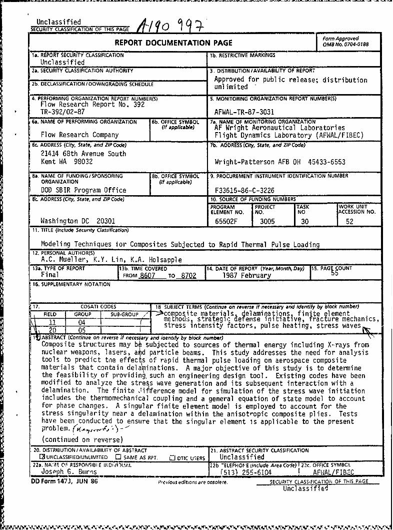
Form ApprovedREPORT DOCUMENTATION PAGE OMB No. 0704-0188

la. REPORT SECURITY CLASSIFICATION lb. RESTRICTIVE MARKINGSUnclassified q

2a. SECURITY CLASSIFICATION AUTHORITY 3. DISTRIBUTION /AVAILABILITY OF REPORT

. DApproved for public release; distribution2b. DECLASSIFICATION/I DOWNGRADING SCHEDULE unl imi ted

4. PERFORMING ORGANIZATION REPORT NUMBER(S) S. MONITORING ORGANIZATION REPORT NUMBER(S)Flow Research Report No. 392TR-392/02-87 AFWAL-TR-87-3031

6a. NAME OF PERFORMING ORGANIZATION 6b. OFFICE SYMBOL 7a. NAME OF MONITORING ORGANIZATION(If applicable) AF Wright Aeronautical Laboratories

Flow Research Company Flight Dynamics Laboratory (AFWAL/FIBEC)6c. ADDRESS (City, State, and ZIPCode) 7b. ADDRESS (City, State, and ZIP Code)

21414 68th Avenue SouthKent WA 98032 Wright-Patterson AFB OH 45433-6553

8a. NAME OF FUNDING/ SPONSORING Bb. OFFICE SYMBOL 9. PROCUREMENT INSTRUMENT IDENTIFICATION NUMBER

ORGANIZATION (If applicable)

DOD SBIR Program Office F33615-86-C-32268c. ADDRESS (City, State, and ZIP Code) 10. SOURCE OF FUNDING NUMBERS

PROGRAM PROJECT TASK IWORK UNITELEMENT NO. NO. NO ACCESSION NO.

Washington DC 20301 65502F 3005 30 5211. TITLE (include Security Classification)

Modeling Techniques ior Composites Subjected to Rapid Thermal Pulse Loading12. PERSONAL AUTHOR(S)

A.C. Mueller, K.Y. Lin, K.A. Holsapple13a. TYPE OF REPORT 13b. TIME COVERED 114. DATE OF REPORT (Year, Month, Day) 15. PAG OUNT

Final IFROM 8607 TO8702 1987 February I16. SUPPLEMENTARY NOTATION

17. COSATI CODES 18 SUBJECT TERMS (Continue on reverse if necessary and identify by block number)

FIELD GROUP SUB-GROUP / ccmposite materils delamioatiQns, finite element1-- 0 methods, strateg i: aefense initiative, Tracture mechanics,1 0 1 stress intensity factors, pulse heating, stress wavesl

1tABSTRACT (Continue on reverse if necessary and ioentify by block number)Composite structures may bo subjected to sources of thermal energy including X-rays fromnuclear weapons, lasers, ahd particle beams. This study addresses the need for analysistools to predict tne effec s of rapid thermal pulse loading on aerospace compositematerials that contain dela1 inations. A major objective of this study is to determinethe feasibility of providing, such an engineering design tool. Existing codes have beenmodified to analyze the stre s wave generation and its subsequent interaction with adelamination. The finite Jif3ference model for simulation of the stress wave initiationincludes the thermomechanical coupling and a general equation of state model to accountfor phase changes. A singular finite element model is employed to account for thestress singularity near a delamination within the anisotropic composite plies. Testshave been conducted to ensure that the singular element is applicable to the presentproblem. , " -

(continued on reverse)20. DISTRIBUTION/AVAILABILITY OF ABSTRACT 21. ABSTRACT SECURITY CLASSIFICATION

1' UNCLASSIFIED/UN LIMITED ] SAME AS RPT. C DTIC USERS Unclassified22a. NA:i CIF R'SPONSIBI E INDIVI')pL 22b "ELEPHOVE (Include Area Code) 22c. OFFICE SYMBCL

Josph G. Burns (513) 255-6104 AFWAL/FIBECDD Form 147J, JUN 86 Previous editions are oosolere. SECURITY CLASSFICATION OF THIS PAGE

Uncl assified

%AAA.n -i -A e_ 0 W W. or-j- ', . r.A kl V% ~- VAWdPr1q.P .kf6 w p ip , R 11 MI k rr -R A K 'r' Rl c

19. ABSTRACT (continued)

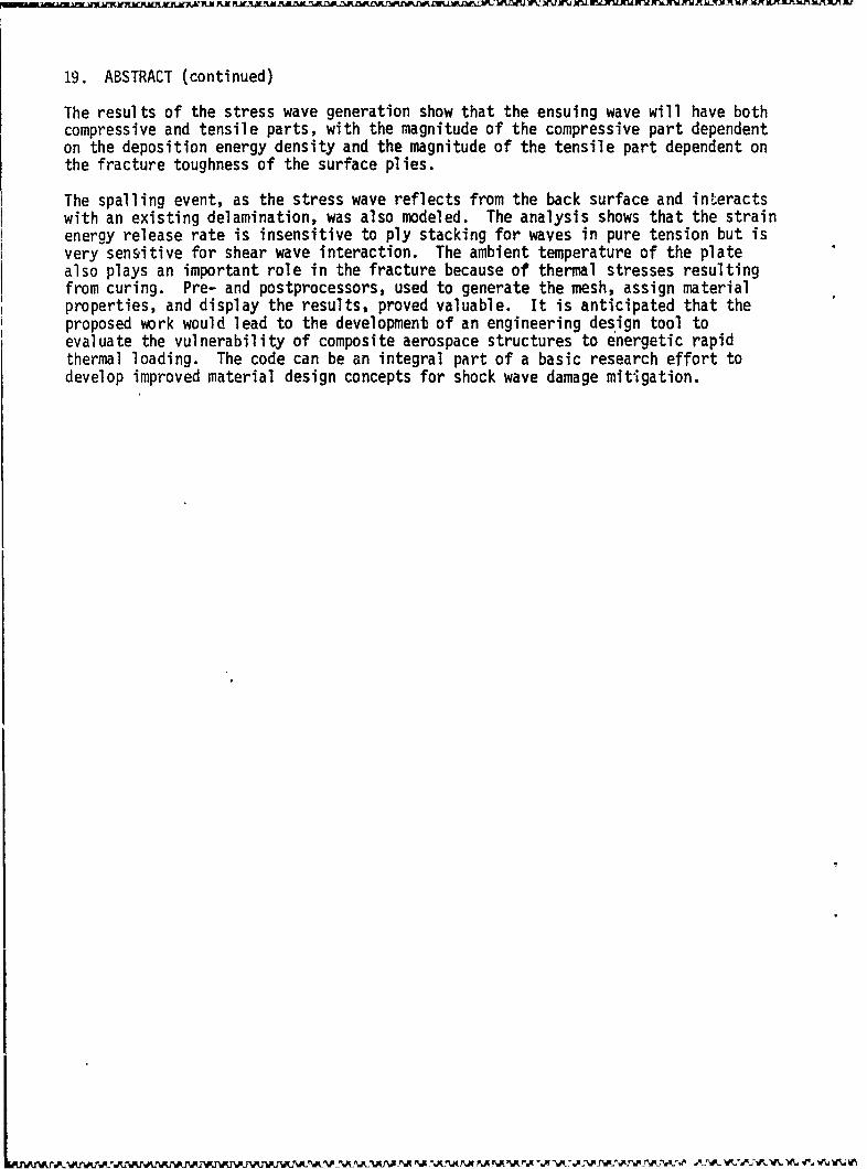
The results of the stress wave generation show that the ensuing wave will have bothcompressive and tensile parts, with the magnitude of the compressive part dependenton the deposition energy density and the magnitude of the tensile part dependent onthe fracture toughness of the surface plies.

The spalling event, as the stress wave reflects from the back surface and interactswith an existing delamination, was also modeled. The analysis shows that the strainenergy release rate is insensitive to ply stacking for waves in pure tension but isvery sen&itive for shear wave interaction. The ambient temperature of the platealso plays an important role in the fracture because of thermal stresses resultingfrom curing. Pre- and postprocessors, used to generate the mesh, assign materialproperties, and display the results, proved valuable. It is anticipated that theproposed work would lead to the development of an engineering design tool toevaluate the vulnerability of composite aerospace structures to energetic rapidthermal loading. The code can be an integral part of a basic research effort todevelop improved material design concepts for shock wave damage mitigation.

L -M -M -M -'EhJN -M -M -M -M -M -MN M N MN ER1JN M. ~. . M~'~V 2 ~

TABLE OF CORTENTS

Page

1. INTRODUCTION I1.1 The Energy Deposition Phase 1

1.2 The Initial Thermodynamic State 3

1.3 Typical Wave Profiles 6

1.4 Assumptions 8

2. THEORETICAL DEVELOPMENTS 11

2.1 Continuum Mechanics Overview 112.2 Singular Finite Element Formulation 132.3 Strain Energy Release Rate 162.4 Plane Strain Stress-Strain Law 17

3. FINITE ELEMENT VALIDATION TEST 20

3.1 Singular Element Test 20

3.2 Thermal Stress Validation 24

3.3 Static Composite Plate Validation Test 27

3.4 Dynamic Composite Plate Validation Test 29

4. SIMULATION OF THE STRESS WAVE INITIATION 36

5. SIMULATION OF THE STRESS WAVE INTERACTION WITH A DELAMINATION 39

6. UNIFIED MODEL FEASIBILITY STUDY 44

7. CONCLUSIONS 46

REFERENCES 46

Accesion For

NTIS CRA&iD111C AB

D1,;; ib,: tion

il-i

iii

r.Kr r.rJxaA r

LIST Ol FIGURES

Figure Page

1. Phase Diagram for a Typical Metal 5

2. Typical Loading History 5

3. Laser Energy Deposition on a Composite Plate 10

4. Plane Sections of a Lamiinate 19

5. Crack Between Different Isotropic Materials 22

6. Coarse FEAPICC Grid 22

7. Fine FEAPICC Grid 23

8. FEAMOD Grid 23

9. Normal Stress FEAPICC Coarse Grid 25

10. Normal Stress FEAPICC Fine Grid 25

11. Normal Stress FEAMOD Solution 26

12. Thermal Stress Test Problem 26

13. Composite Grid 28

14. Normal Stress (t = 0.15 us) 31

15. Normal Stress (t = 0.3 Us) 31

16. Normal Stress (t = 0.35 1s) 32

17. Normal Stress (t = 0.4 Us) 32

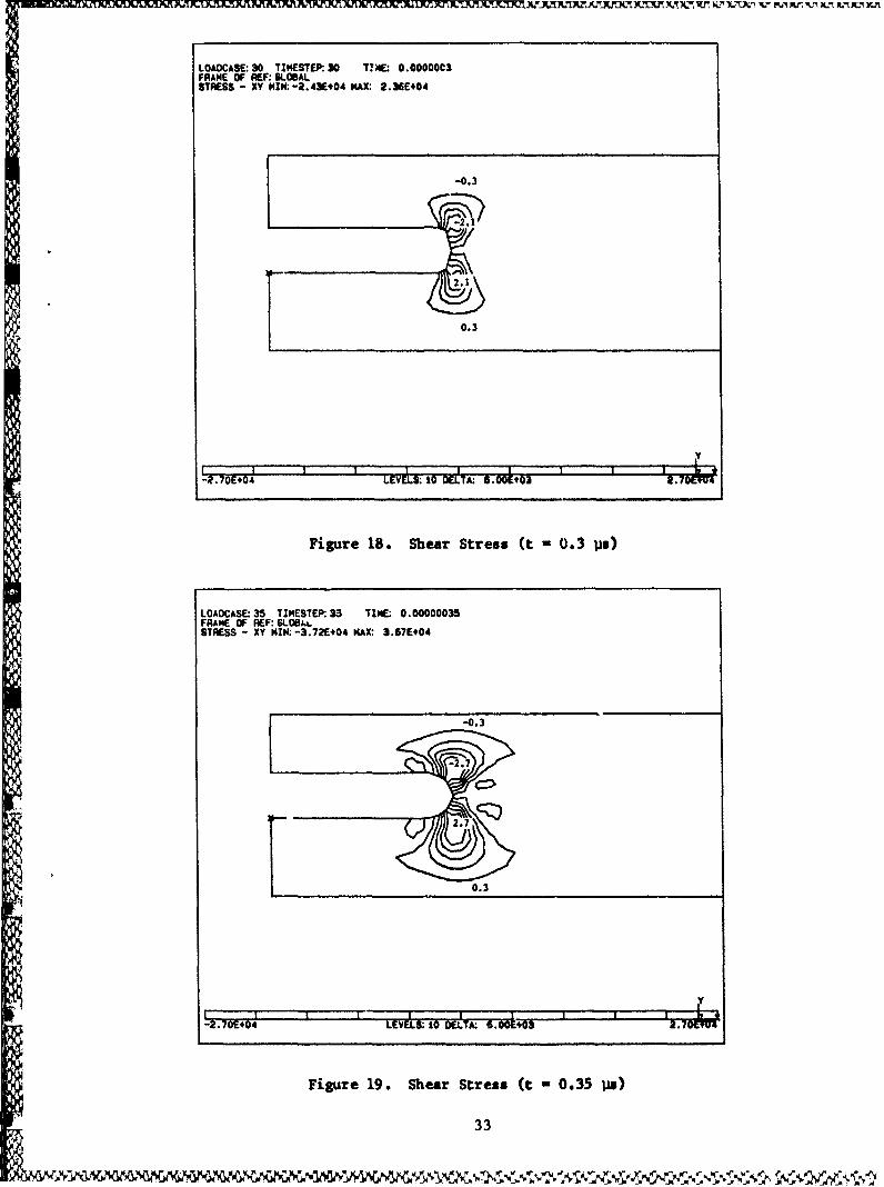
18. Shear Stress (t = 0.3 ts) 33

19. Shear Stress (t = 0.35 iUs) 33

20. Shear Stress (t = 0.4 s) 34

21. Longitudinal Normal Stress (t = 0.3 Us) 34

22. Longitudinal Normal Stress (t = 0.35 is) 35

23. Longitudinal Normal Stress (t = 0.4 ps) 35

24. Initial Fully Developed Stress Wave (t = 0.1 ps) 38

25. Stress Wave Just Before Free Surface Reflection (t -- .7 ips) 38

26. Velocity Vector at Maximum Stress Intensity (t = 0.16 go) 42

27. Normal Stress in the Singular Element (t 0.16 Us) 42

28. Shear Stress in the Singular Element (t = 0.16 ps) 43

29. Von Mises Stress in the Singular Element (t = 0.16 us) 43

iv

LIST OF TABLES

Table Page

1. Stress Intensity Model Comparison 21

2. Static Thermoelastic Tes!: Case Comparison 27

3. Material Properties Along the Principal Coordinates 28of the Fiber Direction

4. Static Composite Ply Stress Intensity Factors 29

5. Dynamic Parametric Tests 40

I!-aiV

1%1,.*i~ -v

1 INTRODUCTION

The physical problem we are addressing in this study is the rapid deposi-

tion of thermal energy on the surface of a composite plate within which a

delamination exists. The high energy flux will stress and perhaps vaporize the

surface plies, and a shock stress wave is initiated through thermal expansion

and the momentum imparted by the blowoff. As this compressive wave initially

passes the delamination, the crack will tend to close and the wave will simply

pass through. But as the wave reflects off the bottom free surface, it will

return as a tensile wave. This wave will open the delamination and produce

excessive stresses at the crack tip. The high stress field could conceivably

cause the delamination to grow and result in the catastrophic failure of the

plate. In addition to the initiation of a longitudinal stress wave, a shear

wave may ensue from a nonuniform spatial distribution or edge effects of the

laser energy flux. Matters are further complicated by the anisotropic and

nonhomogeneous makeup of the composite plate. Hence, the longitudinal andshear waves will propagate at speeds dependent on the ply orientation.

Several time scales may be identified. The energy deposition typically

occurs within hundredths of a microsecond. Depending on the wavelength of the

source, the energy may be deposited on just the surface or throughout the

plate, but in either case it results in an almost instantaneous change in the

temperature. This rapid rise in temperature may produce a phase change at the

surface. Subsequently, the pressure in the gas phase becomes very high, and

the adjacent solid portion responds with a stress wave. This wave will

traverse the thickness of the plate on the order microseconds. The conduction

of heat takes place over a much longer time scale. For example, a temperature

change of 1% requires on the order of 100 milliseconds.

1.1 The Energy Deposition Phase

The analysis tools required for the study of composite structures subjected

to rapid thermal pulses are conveniently considered in three parts, two of

which are analyzed in some detail in this study. The first part is the deter-

minaticn of the nature of the thermal pulse from knowledge or assumptions

about the source of that pulse, which is only discussed in generalities here.

Sources of interest include laser weapons, nuclear weapon X-rays, particle

beams, and other energy sources. The analysis of this part of the problem

must consider the interaction of an clectromagnetic source with the material

of the composite structure and must analyze the subsequent radiation transport

in that material. Analysis techniques are available, but experimental data

sufficient to define material properties for energy deposition in polymeric

materials characteristic of composites are sparse or nonexistent.

The outcome of a study of this radiation transport is a time-position

profile of the thermodynamic state of the composite structure. Fortunately,

to study and develop the tools required for the remaining two parts of the

problem, it is not necessary to have specific numerical results. Rather, it

is only necessary to know the general nature of the results so that the tools

for the rest of the analysis are sufficient to cope with the range of possibi-

lities. A short discussion of the general nature, and of the differences due

to the variety of possible source types, is given.

It is convenient to classify energy sources according to their range of

initial spatial influence and their temporal duration. The best studied

source is the detonation of a nuclear weapon near a structure of interest.

The predominant energy of a modern fusion device is in a substantial X-ray

output that impinges on, and is absorbed into, the adjacent material. If the

detonation is in the atmosphere, the surrounding air absorbs the energy, and a

blast wave is formed that propagates outward and strikes nearby structures.

Alternatively (and exclusively if there is no significant atmosphere present),

the radiation directly reaches a nearby structure. The energy is then absorbed

by the material in the structure.

The time scales of this energy transport phase are typically very short in

comparison to the other significant time scales of the problem. In many cases,

it is considered instantaneous. The characteristic depth of the energy deposi-

tion depends markedly on the composition of the structure. Materials with high

atomic numbers absorb the energy in very shallow depths, while so-called

"low-Z" materials have much greater absorption depths.

Thus, energy deposition due to nuclear devices is typically of very short

duration. The depths of deposition can be either thin compared to structural

dimensions (e.g., a skin thickness of a missile) or of that same size.

When considering laser weapons, there are important differences in this

picture due to the longer wavelengths of the radiation. The time scales, for

a single pulse, are still short. However, the deposition thicl.ness is very

small and, as a result of the very high energy densities, it will vaporize and

"blow off" on a short time scale, which can have a significant quenching effect

2

Ar J kN.rAP rAA',A. "T _%A-.1ANAKR~AAA % A fA .RrhArux~. % A %.AMA IR?5. A x'%A ",%A ?%.A - .A Wt. A I Wlk,%K,

on the energy deposition itself. In this case, there can be important inter-

actions between the thermodynamics of the material, the resulting wave actions,

and the energy deposition itself. For that reason, multiple and rapidly pulsed

weapon outputs are under consideration. The tools to be developed here must

be able to handle this important case.

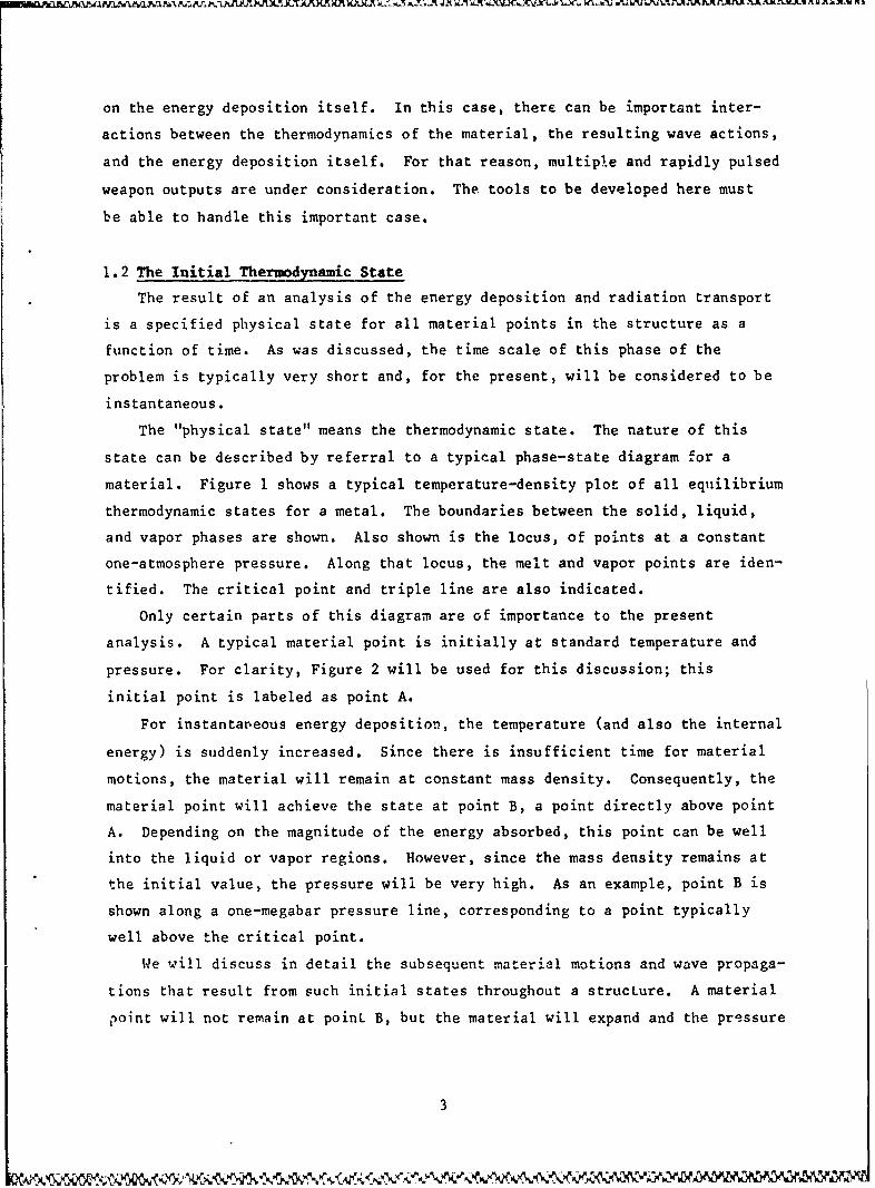
1.2 The Initial Thermodynamic State

The result of an analysis of the energy deposition and radiation transport

is a specified physical state for all material points in the structure as a

function of time. As was discussed, the time scale of this phase of the

problem is typically very short and, for the present, will be considered to be

instantaneous.

The "physical state" means the thermodynamic state. The nature of this

state can be described by referral to a typical phase-state diagram for a

material. Figure 1 shows a typical temperature-density plot of all equilibrium

thermodynamic states for a metal. The boundaries between the solid, liquid,

and vapor phases are shown. Also shown is the locus, of points at a constant

one-atmosphere pressure. Along that locus, the melt and vapor points are iden-

tified. The critical point and triple line are also indicated.

Only certain parts of this diagram are of importance to the present

analysis. A typical material point is initially at standard temperature and

pressure. For clarity, Figure 2 will be used for this discussion; this

initial point is labeled as point A.

For instantaneous energy deposition, the temperature (and also the internal

energy) is suddenly increased. Since there is insufficient time for material

motions, the material will remain at constant mass density. Consequently, the

material point will achieve the state at point B, a point directly above point

A. Depending on the magnitude of the energy absorbed, this point can be well

into the liquid or vapor regions. However, since the mass density remains at

the initial value, the pressure will be very high. As an example, point B is

shown along a one-megabar pressure line, corresponding to a point typically

well above the critical point.

We will discuss in detail the subsequent material motions and wave propaga-

tions that result from such initial states throughout a structure. A material

point will not remain at point B, but the material will expand and the pressure

3

will reduce eventually back to normal pressure. Since these motions occur

after the energy deposition, they are adiabatic and, as a consequence, the

path followed in this thermodynamic phase space is along an isentrope. A

typical isentrope from point B is indicated. The one shown happens to

intersect the vapor-liquid dome, but it will not if point B is at a

sufficiently high temperature. The final states of the material will

ultimately be at very low densities, and the material will be hot and expanded.

This discussion serves to identify the thermodynamic description and model

that is needed for the initial deposition phase for an analysis of the type

studied here. A relatively precise description of all states at nominal and

lower densities is needed. A model of the phase boundaries and the shape of

the pressure curves and adiabats (isentropes) in this region is also needed.

Subsequent wave motions can introduce further states. In the case that a

layer of surface material vaporizes and blows off at high velocity, or a thin

layer of material is spalled off, then a shock wave will be generated that

propagates into the interior of the structure. This shock wave is similar to

one that would be generated by an impact at the surface. The resulting shocked

states lie along a Hugoniot curve centered at the initial point of the

material. A typical Hugoniot curve from the standard temperature and pressure

is also shown in Figure 2. We can see that these states are at higher than

normal density and temperature.

In the case of composite materials, specific data on these thermodynamic

states are very sparse. In the present Phase I study, a thorough literature

search has not been conducted, but preliminary investigations uncovered only a

very few thermodynamic properties, including only the initial density, the

Gedneisen parameter, the wave speed, and thermal expansion at standard

temperature and pressure. No data were found on temperature states above a

few hundred degrees, and none describing phase-change mechanisms. Clearly,

before we can have sufficient confidence in energy deposition studies, much

more work is needed in this area: both analytical descriptions of the

thermodynamics of composite materials and experimental tests to verify and

calibrate those analytical models. The additional features arising from the

multiple-constituency of the composite materials will also require further

investigation.

4

VAPOR

CRITICAL POINT

LIOUIO

VAPOR POINT

LIOUID/VAPOR

SOLID

TRIPLE POINT LINE MELT POINT

P:I ATM

S.T.P.

MASS DENSITY PFigure 1. Phase Diagram for a Typical Metal

8

00

HUGON IOTCURVE

A

MASS DE ISITY P

Figure 2. Typical Loading History

.. ).5

1.3 Typical Wave Profiles

To understand the computer results to be shown shortly, we first describe

the general nature of the stress pulses that will arise in the cases of rapid

thermal pulses. An idealized description is given here, followed by a

presentation of some actual code output that includes all of the real physics

of the problem.

For an idealized case, consider a

plate of thickness t in the x direction.

We may assume that there is an QDinstantaneous triangular uniform energy

deposition at the free surface of that

plate, with the maximum value at the

surface and dropping linearly Lo zero

at some depth h less than t.

There is a resulting high pressure

in that deposition region that produces

an initial pressure profile as shown in =____.___

sketch 1. h x

The general effect of this initial

state can be understood by considering

the special case of a linear elastic

material for which superposition holds.

In that case, the bal, ice of linear

momentum reduces to the well-known one-

dimensional wave equation. If the

pulse is not near the free surface,

then the initial pulse shown above

would split into two equal parts, one

traveling to the right at the wave

velocity c, and one to the left. Thus,

a short instant At later, these two

waves look as shown in sketch 2.

However, there is a free surface at

x = 0 to consider. The condition that

the pressure be zero at x = 0 is satis-

fied by adding a third wave, opposite to

6

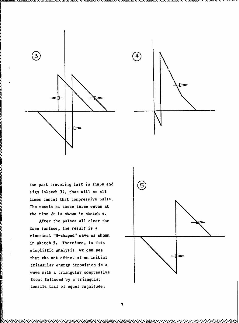
the part traveling left in shape and

sign (sketch 3), that will at all

times cancel that compressive pulsb.

The result of these three waves at

the time At is shown in sketch 4.

After the pulses all clear the

free surface, the result is a

classical "N-shaped" wave as shown__ _

in sketch 5. Therefore, in this

simplistic analysis, we can see

that the net effect of an initial

triangular energy deposition is a

wave with a triangular compressive

front followed by a triangular:

tensile tail of equal magnitude.

7

This analysis assumes instantaneous energy deposition. A slightly modified

picture occurs when the deposition time to is not small compared to the pulse

depth h divided by the wave speed c. In that case, for the same total energy

and deposition depth, the final wave after deposition time will have a reduced

peak and will have a total spatial width of h + ct . However, there will still

be a following tensile tail of the same magnitude as the compressive front.

Real materials are not linear elastic, particularly at the high temperature

and pressure states encountered during the energy deposition phase. The most

important feature of nonelastic actual behavior will be a finite tensile

strength, due either to the inherent strength of the solid, or due to the

reduced strength of a vaporized or partially vaporized state.

Assume, for example, that the energy deposition magnitude is such that the

peak compressive stress in the above sketches is 5 kilobars, and that the

tensile spall strength in 1 kilobar. Then, at some time between the first

growth of the tensile tail at the free surface and the time when the N-shaped

wave would have left the free surface, the tensile stress at some distance in

from the free surface will reach 1 kilobar, and tensile spall will occur.

Indeed, with the values stated in this simple example, that initial spall

thickness will be exactly one-fifth of the deposition depth h. That reduces

the stress at the spall plane back to zero, and a tensile pulse will again

begin to grow, resulting in a second spall of equal thickness. In the final

analysis, the resulting wave propagating into the structure will have a tensile

tail, but limited in magnitude to the tensile spall strength. In the example

here, that tail would be limited to 1 kilobar.

The final stress wave profile will, of course, depend on the exact nature

of the energy deposition. In a one-dimensional thermoelastic analysis neglect-

ing vaporization and tensile strength, Paramasivam and Reismann (1986)

(Reference 7) find a similar compressive/tensile wave resulting from a

Gaussian deposition in space and time.

1.4 Assuxptions

A complete analysis of this complicated thermomechanical problem is beyond

the scope of this Phase I work, but there are a number of assumptions that may

be made for the problem to become tractable for analysis. First, we tacitly

assume that the energy flux is large enough to vaporize the first few plies

but is not sufficiently strong to vaporize to a significant depth in the

8

plate. If we assume that the delamination does not reside too close to the

upper surface, then the effects of the delamination will not be strongly

coupled to the shock wave initiation. Hence, the interaction of the stress

wave with the delamination may be treated separately fromn the physics of its

initial generation. Furthermore, if we wish to analyze the stresses at the

delamination in a planar setting, we are forced to make some assumptions

regarding the areal extent of the energy deposition and the geometry of the

delamination. We may assume either that the energy is uniformly distributed

over an area much larger than the characteristic width of the delamination, or

that the energy is deposited uniformly over a thin but very elongated region.

The first assumption seems more realistic, but the second allows us to study

effects related to the position of the energy deposition with respect to the

delamination. The delamination itself must be regarded as having some large

extension down the plate. In other words, the delamination is a long cavity

with small width and even smaller thickness. With these assumptions, the

deformation is uniform along the long axis of the delamination (and the energy

deposition area), and the plate exists in a state of plane strain (Figure 3).

The assumption of a large uniform energy deposition further reduces the

dynamics of the stress wave propagation to a one-dimensional problem, since the

effects of the crack do not interact. Also, since the uniaxial stress-strain

relation is independent of the ply orientation, the stress wave propagates as

in a homogeneous material. It is only after the stress wave interacts with

the delamination that the orthotropic, nonhomogeneous properties become

apparent. Accordingly, if we assume that the initial stress wave is entirely

compressive, and the closed delamination cannot slip (infinite friction), then

the compressive wave will pass through unchanged.

With these assumptions, the problem may be appreached with the two existing

codes, FEAPICC, a two-dimensional, finite element code for propagating cracks

between differing anisotropic materials, and WONDY, a one-dimensional, finite

difference code modeling the thermomechanics of the energy deposition. Before

moving on to a discussion of the simulations using these codes, the next

section presents more details of the theoretical model.

9

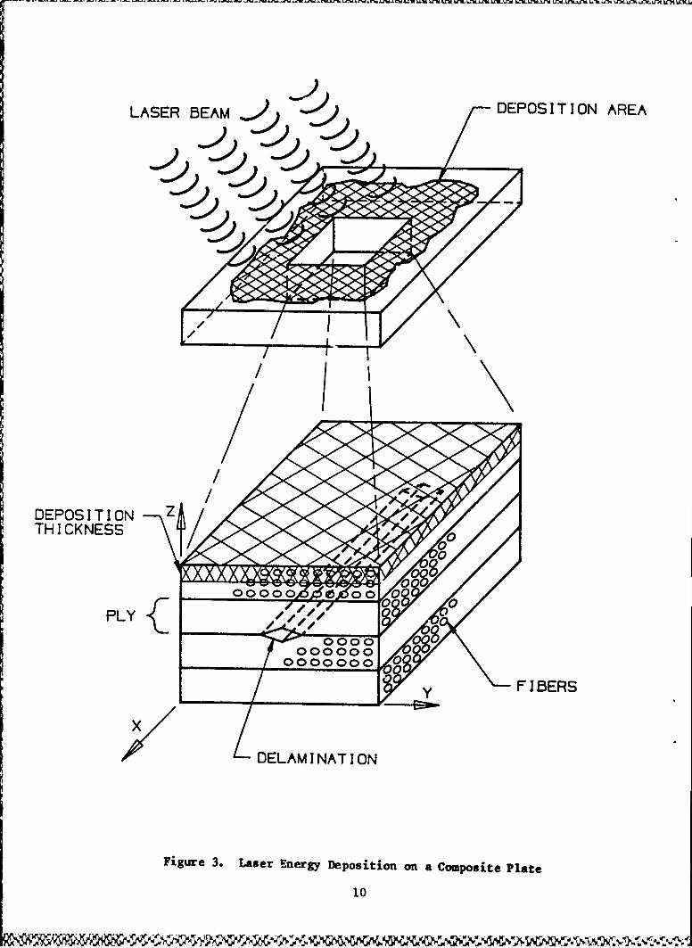
LASER BEAM DEPOSITION AREA

DEPOSITION Z)TH ICKNESS

100

2. T!,-ZTICAL DEVEWPMENTS

2.1 Continuum Mechanics Overview

We present here a brief description of the continuum model with emphasis

on particular aspects that relate to the deposition of energy in composite

lami.lates.

The motions are governed by the general equations of continuum mechanics,

as are used in all studies of fluid, solid and structural mechanics. The

computer codes used in this and other studies transcribe those equations into

an approximate form suitable for solution on a computer.

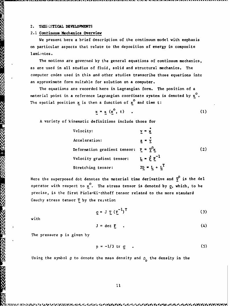
The equations are recorded here in Lagrangian form. The position of a

material point in a reference Lagrangian coordinate system is denoted by x.

The spatial position x is then a function of x and time t:

xx (x°, t) (1)

A variety of kinematic definitions include those for

Velocity: v = x

Acceleration: a n

Deformation gradient tensor: F = V0x (2)

Velocity gradient tensor: L = i F-

Stretching tensor: 2D L + LT

Here the superposed dot denotes the material time derivative and V is the del

operator with respect to x0 The stress tensor is denoted by q, which, to be

precise, is the first Piola-Ki-chhoff tensor related to the more standard

Cauchy stress tensor T by the reiqtion

a J T (F-lT (3)

with

J det F . (4)

The pressure p is given by

p -1/3 tr . (5)

Using the symbol p to denote the mass density and p the density in the

XA

J . ~ J ~ ~ R .HPH,. .Ar.r...I ~ ~ JdJU VJ '~~ ' ~C. . .. V JWJ ' . ~~. ~ ~ PiA ~ l 'jM~

reference configuration, the balance of mass can be written as

; +, (6)

the balance of linear momentum as

V°o + P : o (7)

and, finally, the balance of energy as

pe = tr(TD) -V.%+ pr , (8)

where b is the body force, % is the heat flux vector and r is the deposited

energy per unit mass.

These equations are supplemented by the constitutive equations describing

the material. There is a relation between the internal energy e, the density p

and the pressure p, which we write as

p = p(e, p) (9)

While this single equation of state form is sufficient to describe completely

the thermodynamics, it is more common to also include descriptions for the

temperature T and entropy n:

T = T(e, p)(10)

n = n(e, p)

Then these three thermodynamic equations can be solved to use any two thermo-

dynamic variables as independent. The discussions of the previous section used

T and p; the corresponding forms are given by

p = p(p, T)

e = e(p, T) (11)

n -n(p, T)

and constant pressure or constant entropy states lie along some curve in p - T

space as described above. Phase boundaries become curves in this p - T space.

To complete the description, a relation for the shear stress components is

needed. This usually takes the form of equations for the stress deviator tensor:

2D = 2-p C • (12)

Relating the rate of change of 2D to the stretching tensor D via a shear

modulus G is usual. The shear modulus G can depend on the thermodynamic state,

12

Ll- . -' d. Ad _1% -'% .fW'J N, LN V*' 0A %A JN U ~ N VA %.N LNfr vJw V* LN15 L VK%.~V,( X N .I V . N -LNLNVJ 'W UXP % ~XNvV'NVW t'

~~~~1J!JwV~iW X ' V W W ' WWh~~ U V R- V FW WW W

i.e., the temperature and density. Plasticity relations are used to limit the

values of the stress deviators when plastic flow occurs; the yield strength Y is

also dependent on the thermodynamic state. Polymeric materials of composite

structures may require more general and time-dependent models. Again, little is

presently known about suitable models. The most that appear to be available are

quasi-i;atic dependences of strength and stiffness versus temperature, and only

to the few hundred degrees for which composite materials maintain their primrry

structural integrity. Finally, fracture criteria are needed to ,describe spall

(tensile failures) vnd, in the case of composite structures, ply delaminations.

It is clear that there is an imposing amount of information that goes into

the final solution of these problems. Fortunately, there are well developed

and tested finite difference codes, such as the one-dimensional code WONDY and

the two-dimensional code CSQ that have been used in the present program.

Provisions for a number of different material model types are available, as

well as both analytical and tabular descriptions of the thermodynamics,

including complete three-phase boundary descriptions and transitions. At the

present, for normal wave-propagation studies, it must be said that the models

are better developed than warranted; however, the experimental data to provide

inputs to these models (or even to simply discover what type of a model is

appropriate) are lacking. Furthermore, even for generic input models, the

effects of composite laminations or delaminations on the wave propagation

mechanics has not been considered. It is, of course, that issue that is the

primary focus of the present study.

2.2 Singular Finite Element Formlation

In the present study, singular finite elements are used near the tip of a

delamination crack to account for stress singularity at the crack tip. These

elements incorporate stress and displacement fields from the closed-form

solutions and therefore are extremely accurate and efficient. The singular

elements are then combined with the regular isoparametric elements in the

surrounding region so that the standard finite element procedures can be used

to obtain displacement at each node.

The development of singular elements is based on a hybrid functional

derived in Tong et al. (1973) (Reference 10). This hybrid functional was used

by Lin and Mar (1976) (Reference 5) for the study of bi-material crack problems

and recently by Aminpour and Holsapple (Aminpour, 1986) (Reference 1) for the

13

uN L' LPW JN UN L fW "V r JNil~ LJrVVV ~fV tU ,A WN JW KUNMLM WN 1 . . WX V ~ A ~ A I .M '-A A 'NN~ '%. M A -- "U " IM &X%X"F ! A r SA

dynamic analysis of cracks between two anisotropic materials. For a two-

dimensional continuum divided into m elements, the hybrid functional can be

defined as

~ (13)where

= °( e(y+ Go) _ pub+ - dV

tf (14)

+ f u- v).t ds - u.*Tds dt

in o

0In the above, y, E, a , and u are the stress, strain, thermal stress and dis-

placement, respectively. Otner variables are the body force b, the density p

and the tractions T and r on the boundaries. The displacement v along the

interelement boundary S. is as- umed independently of the interior displacementin

u. The constraint integral over S. is added to enforce the continuity of the~ indisplacements between the singular element and a regular element that uses

different interpolation functions for the displacement components.

Making use of the stress, strain, and displacement fields obtained from the

closed-f m solution of a semi-infinite crack, we can assume

1u = U13

a = AE 2 + o (15)

T= R3

where the 13's are unknown constants to be determined from the finite element

solution of the overall problem.

If the field variables in Equation (15) are used, then all elasticity

equations are satisfied exactly at any time t, and the volume integral in the

hybrid functional can be reduced to a boundary integral. The Euler equation

for the variational functional is simply

U =v on S.on S in

and (16)

T nao on S--- 0

where n is the normal vector.

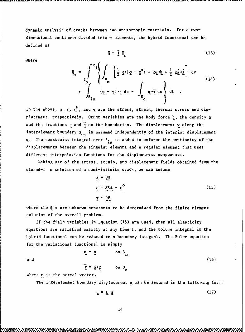
The interelement boundary disilacement u can be assumed in the following form:

u.= 9(17)

14

in which I is the nodal displacement vector, and L is chosen such that u is

comp't. '.le with the surrounding regular elements. For example, L may be

chosen to vary linearly between two nodes along the interelement boundary if

constant strain elements are used in the surrounding.

Substituting the assumed quantities from Equations (15) and (17) into

the hybrid functional and taking the variation of the functional with respect

to B, we obtain (Aminpour, 1986) (Reference 1)

B B qi with BP I G (18)

and

hM= - -T T ) dt (19)t

where 0

K B T - T M T * T

- -1- --2E- 2B M3 B

TM B-2 - (20)

V = BT2+ TM3 B

F BTF

- -s .

Ti, remaining matrices are defined as follows:

fETf dvJm

Fs u- ) dv

1 VM

12 = fV uTpu dv (21)

Mz f 'p dv~ Vm

G = - RTL dsin

fin RTUd

2 15

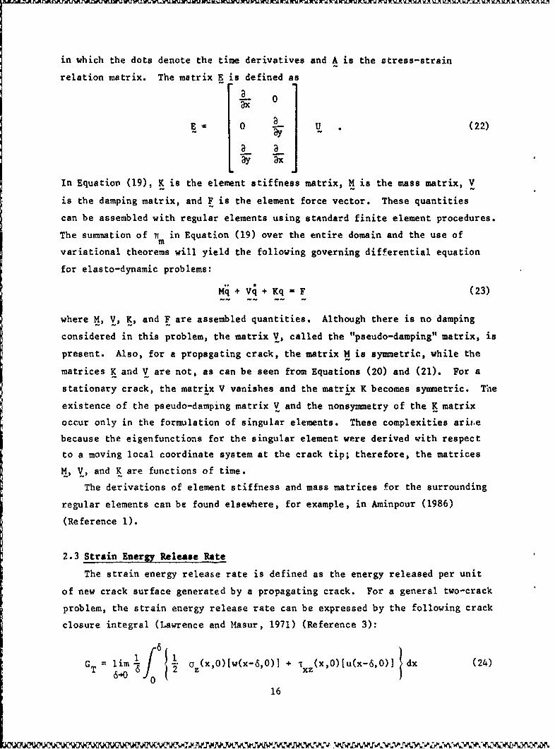
in which the dots denote the time derivatives and A is the stress-strain

relation matrix. The matrix E is defined as

0

E 0 U . (22)

a a

In Equatiov (19), K is the element stiffness matrix, M is the mass matrix, V

is the damping matrix, and F is the element force vector. These quantities

can be assembled with regular elements using standard finite element procedures.

The summation of 7t in Equation (19) over the entire domain and the use ofm

variational theorems will yield the following governing differential equation

for elasto-dynamic problems:

Mq + V + Kq = F (23)

where M, V, K, and F are assembled quantities. Although there is no damping

considered in this problem, the matrix V, called the "pseudo-damping" matrix, is

present. Also, for a propagating crack, the matrix M is symmetric, while the

matrices K and V are not, as can be seen from Equations (20) and (21). For a

stationary crack, the matrix V vanishes and the matrix K becomes symmetric. The

existence of the pseudo-damping matrix V and the nonsymmetry of the K matrix

occur only in the formulation of singular elements. These complexities arite

because the eigenfunctions for the singular element were derived with respect

to a moving local coordinate system at the crack tip; therefore, the matrices

M, V, and K are functions of time.

The derivations of element stiffness and mass matrices for the surrounding

regular elements can be found elsewhere, for example, in Aminpour (1986)

(Reference 1).

2.3 Strain Energy Release Rate

The strain energy release rate is defined as the energy released per unit

of new crack surface generated by a propagating crack. For a general two-crack

problem, the strain energy release rate can be expressed by the following crack

closure integral (Lawrence and Masur, 1971) (Reference 3):

GT lim o(X,O)[w(x-6,0)I + r (x,0)[u(x-6,O)] dx (24)

16

' F ','x " O ' ' 4 , ;',, , , 9 e' "' " % ' ,,",. ",. " lW''F " .. ,. IIw NAIW -'IX %A '", ,W

where the firct term in the integral can be defined as G (mode 1) and the

second term as 02 (mode 2). The stresses are evaluated at a distance x ahead

of the crack tip and the corresponding displacements are calculated at a distance

6 - x behind the tip of a crack.

In the presetit study, the stress and displacement are obtained from an eigen-

function expansion method with each term accurate to a constant 0.. The 8

matrix is then determined by matching the local crack-tip solution (singular

elements) with far-field solutions (regular elements). Once B's are found, the

stresses and displacements are known, and Equation (24) can be integrated

numerically. Note that since the stress or strain is oscillating near the tip

of an interface crack between two different materials, the G1 and G2 results as

obtained from Equation (24) generally depend upon the 6 values chosen (Froula

et al., 1980) (Reference 2). Therefore, the usefulness of separate G1 , G2

values for bi-material crack problems remains to be studied. However, the total

strain energy release rate GT has been shown to be independent of 6 (Walker

and Lin, 1987) (Reference 11).

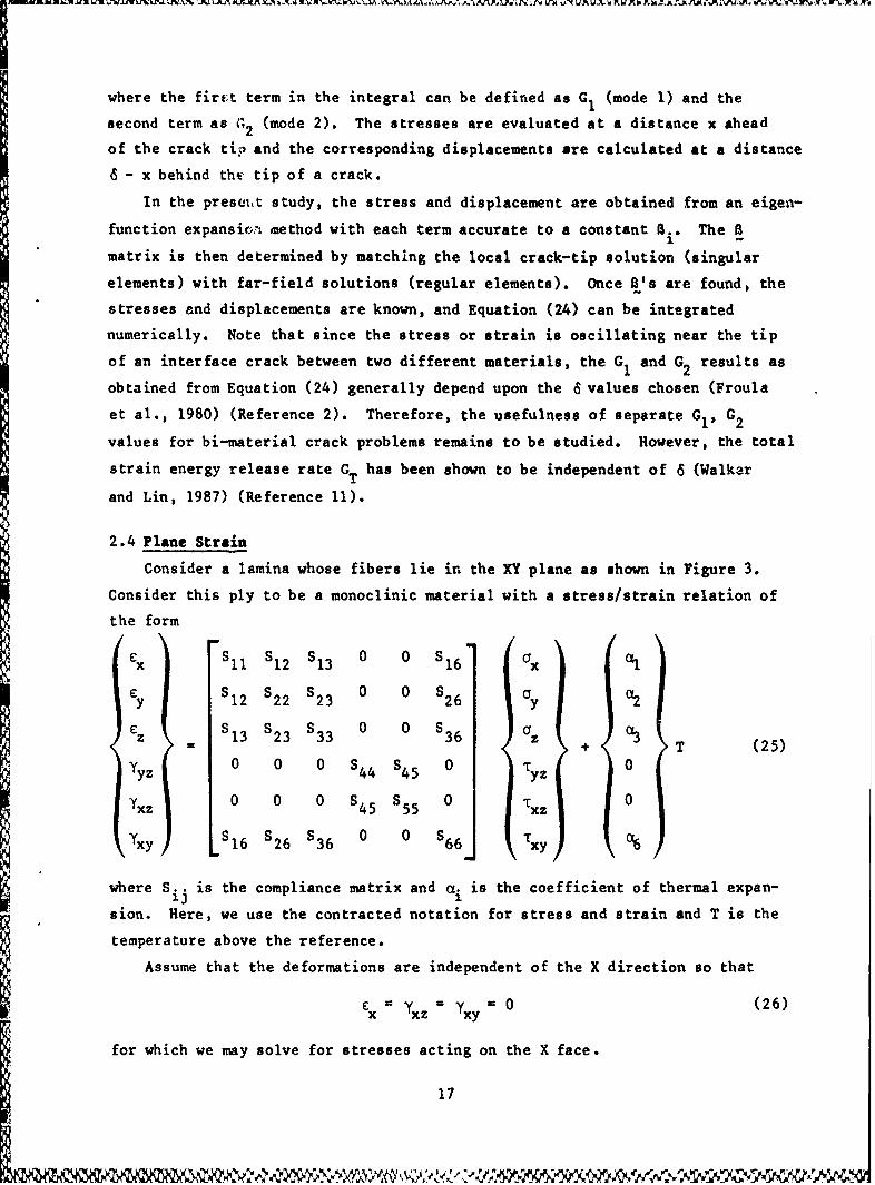
2.4 Plane Strain

Consider a lamina whose fibers lie in the XY plane as shown in Figure 3.

Consider this ply to be a monoclinic material with a stress/strain relation of

the form

x Sl S12 S13 0 0 S 16 lx

Cy S1 2 S2 2 S23 0 0 $26 ay O2

z ,, 13 $23 S33 0 0 S 36 (Z + 3 T (25)

Yyz 0 0 0 $4 4 S4 5 0 Tyz 0

YxZ 0 0 0 S45 S55 01 xZ 0

Yxy LS16 $26 $36 0 0 S66] Txy

where Sij is the compliance matrix and ai is the coefficient of thermal expan-

sion. Here, we use the contracted notation for stress and strain and T is thetemperature above the reference.

Assume that the deformations are independent of the X direction so that

Ex = Yxz ='xy =0 (26)

for which we may solve for stresses acting on the X face.

17

1I (S S -S S )or + (S S -s S ) + (S - )

x d 16 26 - 66 12 y 16 36 - S6613 )az 16% - S661)T

=1

y d 1 l2S16 - 511526)0y + (s 1 6 S 1 3 - S3 6Sl)oz + (S1 6 (1. - S1 1 %)T (27)

S45

Ixz S 55 y'

with

dS2 (28)11 66 16

Substituting these expressions back into the three-dimensional stress/strain

relations and adopting the two-dimensional stress/strain definition as

E b bl2 0y

E: z - b12 b22 0z + z T (29)

yZ L 0 0 b 33 T 0

then

b S22 + (2 S- $66S2 - S2 )/db 22121626 S66 12 11 26

b ( SSS2 S 2 )/22 $33 + (2 S13S636 - 66 13 - SIIS36)/d

= $23 + (S16S12S36 + S16S26S13 - $66S13S12 - S26S36)/d

(30)

b =S S2 /S33 44 45 55

+ (S 2 6 s1 6 - s6 6S

1 2 ) 0 + (s 12 s 1 6 - 26 s 11)a 6

a 03 (s 36 s 16 - s 6 6 S 1 3 ) + (s 1 3s 1 6 - s 3 6 S 1 1 )

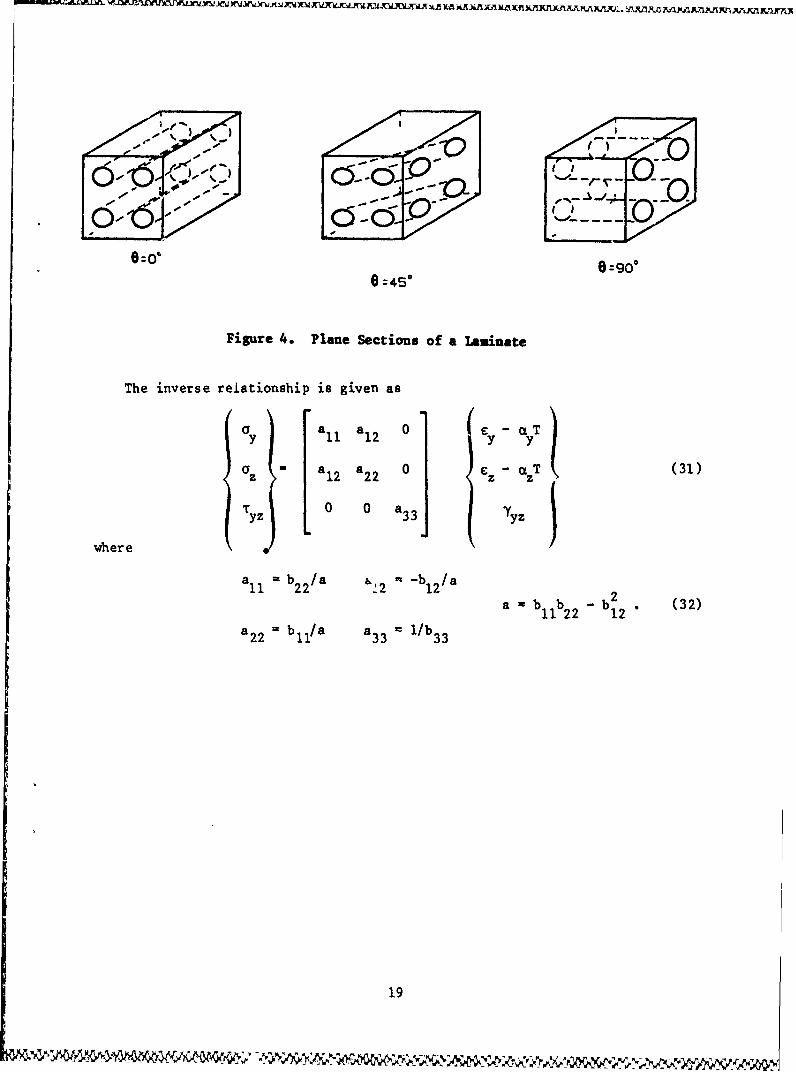
Note that under the plane strain assumption, the material behavior becomes

orthotropic. This is as expected, since, depending on the orientation of the

fibers, the YZ plane cuts the fibers in circles, ellipses, or straight lines,

as seen in Figure 4.

18

0., C5- - U1

0 1 8=900=450

Figure 4. Plane Sections of a Laminate

The inverse reiationship is given as

a 11 12 0 ( - 'Ia = a 12 a22 0 -ctT (31)

Tyz 0 0 a33 Yyz

where

a I1 b 22/a ,.2 "-b 2/a

a b -b . (32)

a22 = b/11 a a33 1/b 3 3

19

3. FINITE ELKMNT VALIDATION TEST

In order to carry out this study, the FEAPICC code was transported from a

CDC 60-bit computer to the Apollo 32-bit machine. This necessitated converting

the code from single precision to double precision. However, since no double-

precision complex arithmetic is available on the Apollo, most of the singular

element computations were left in complex form with no apparant loss in

precision. Conversion to double precision was especially important for dynamic

problems and problems with many unknowns.

In addition to these conversion problems, new theoretical developments and

applications and new I/0 formats necessitated other modifications that required

testing. This section documents tests performed to validate the accuracy of

the code.

3.1 Singular Eleient Teat

This section investigates the accuracy of the singular element when its

dimensions become small compared to the size of the delamination. A typical

ply thickness of a composite is on the order of 0.005 inch, while the delamina-

tion itself may be as large as 1 inch. Although nondestructive tests would

rule out such a large delamination, it is conceivable that a delamination could

grow to such lengths under normal operating conditions. To represent the

stress variation properly, one or two elements would be required to lie. within

each ply. We find that the ratio of the crack length to the singuler element

size may be very large. A simple static analysis shows that the stresses grow

by the square root of the ratio of the crack length to the dis-

tance to the crack tip. If the singular element occupies such a small region

around the crack tip, this means that regular isoparametric elements next to

the singular element must resolve large stress gradients.

O'Leary (1981) (Reference 6), in a one-dimensional error analysis and

supporting numerical studies, shows that as the singular element becomes small,

the error, in the energy norm, converges to zero. However, the rate of conver-

gence suddenly slows after the singular is reduced below a certain size. The

rate of convergence then becomes that which would be expected if no singular

element was employed. The error in the stress intensity factor shows similar

behavior except that no convergence is observed after the singular element is

reduced below a certain size. In any case, the errors were significantly

improved by the use of the singular element over computations that employed no

20

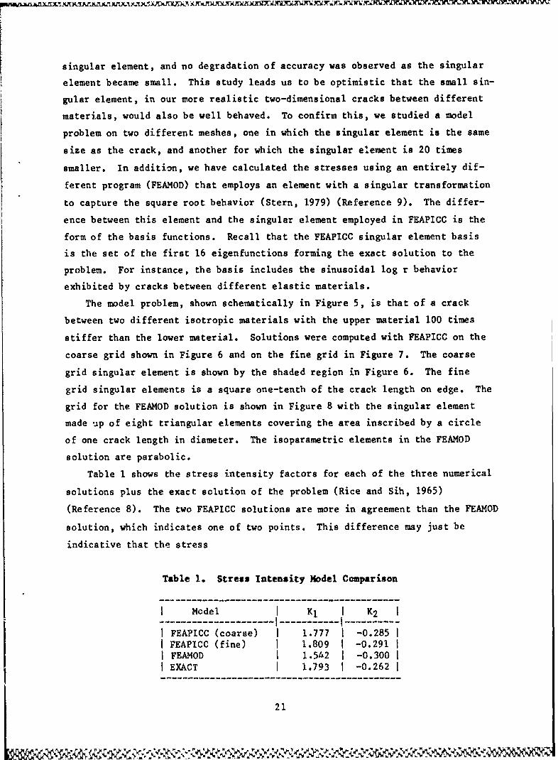
singular element, and no degradation of accuracy was observed as the singular

element became small. This study leads us to be optimistic that the small sin-

gular element, in our more realistic two-dimensional cracks between different

materials, would also be well behaved. To confirm this, we studied a model

problem on two different meshes, one in which the singular element is the same

size as the crack, and another for which the singular element is 20 times

smaller. In addition, we have calculated the stresses using an entirely dif-

ferent program (FEAMOD) that employs an element with a singular transformation

to capture the square root behavior (Stern, 1979) (Reference 9). The differ-

ence between this element and the singular element employed in FEAPICC is the

form of the basis functions. Recall that the FEAPICC singular element basis

is the set of the first 16 eigenfunctions forming the exact solution to the

problem. For instance, the basis includes the sinusoidal log r behavior

exhibited by cracks between different elastic materials.

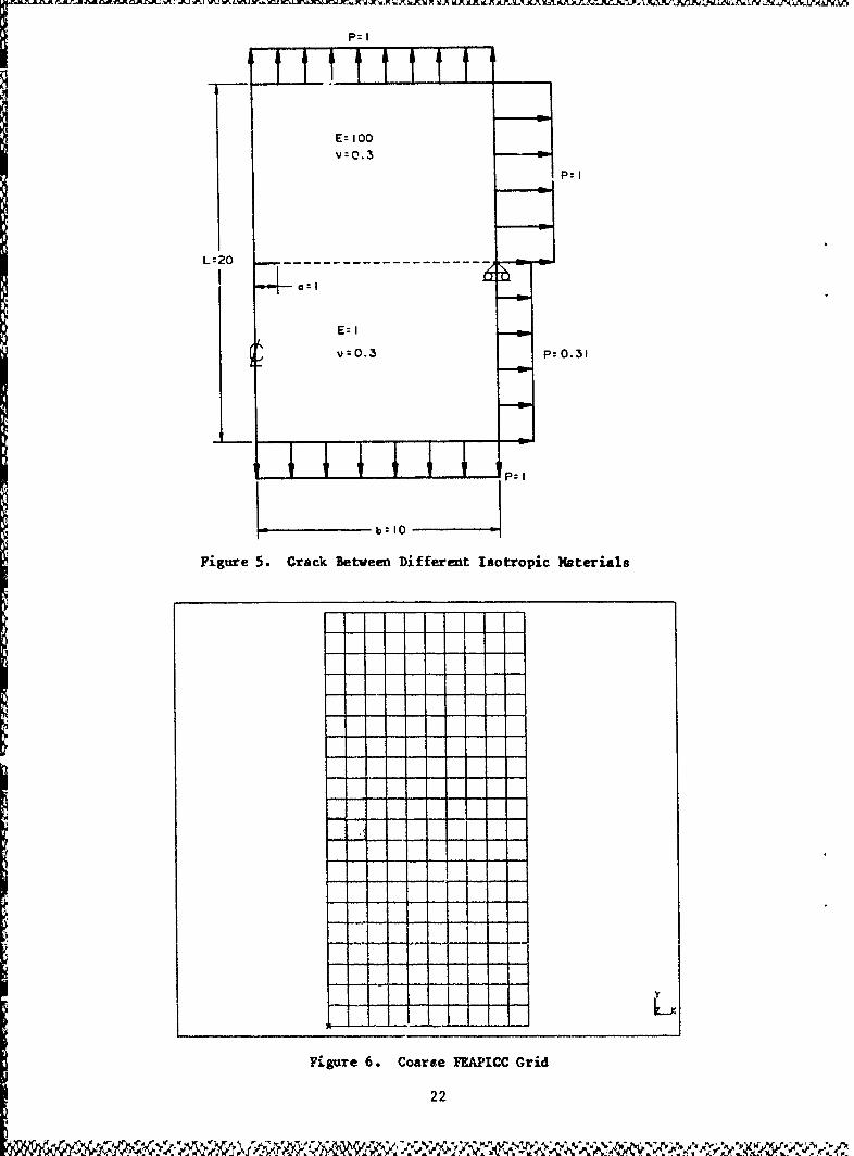
The model problem, shown schematically in Figure 5, is that of a crack

between two different isotropic materials with the upper material 100 times

stiffer than the lower material. Solutions were computed with FEAPICC on the

coarse grid shown in Figure 6 and on the fine grid in Figure 7. The coarse

grid singular element is shown by the shaded region in Figure 6. The fine

grid singular elements is a square one-tenth of the crack length on edge. The

grid for the FEAMOD solution is shown in Figure 8 with the singular element

made up of eight triangular elements covering the area inscribed by a circle

of one crack length in diameter. The isoparametric elements in the FEAMOD

solution are parabolic.

Table 1 shows the stress intensity factors for each of the three numerical

solutions plus the exact solution of the problem (Rice and Sih, 1965)

(Reference 8). The two FEAPICC solutions are more in agreement than the FEAMOD

solution, which indicates one of two points. This difference may just be

indicative that the stress

Table 1. Stress Intensity Model Comparison

I Model K1 I K2------------------- ----------- ----------

I FEAPICC (coarse) 1.777 -0.285 II FEAPICC (fine) 1.809 -0.291 II FEAMOD I1.542 -0.300 II EXACT 1.793 -0.262 I

21

P= I

Ez- 100v -0 .3

P

: I

0.O3 P= 0. 31

i A P: I

b: 10

Figure 5. Crack Betweeni Different Isotropic Materials

Figuire 6. Coarse FEAPICC Grid

22

%

Figure 7. Fine FEAPICC Grid

Figure 8. FEAMOD Grid

23

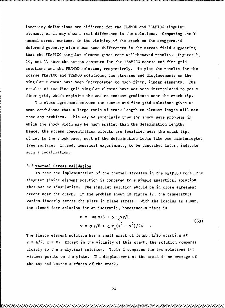
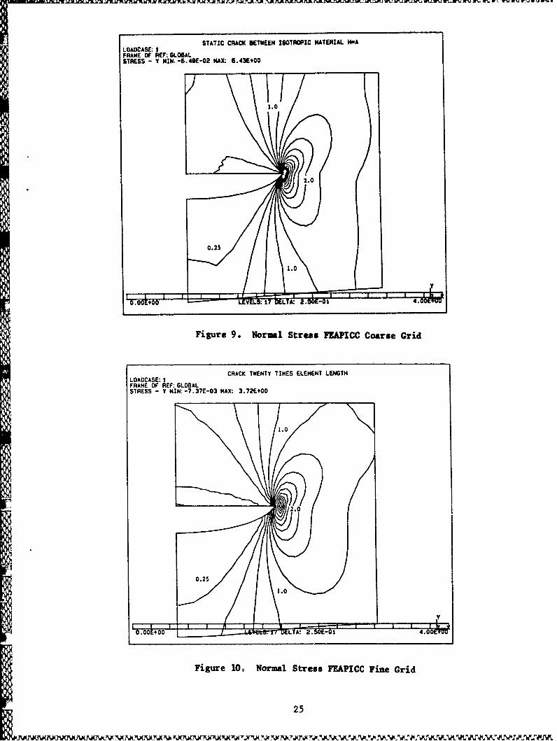
intensity definitions are different for the FEAMOD and FEAPICC singular

element, or it may show a real difference in the solutions. Comparing the Y

normal stress contours in the vicinity of the crack on the exaggerated

deformed geometry also shows some differences in the stress field suggesting

that the FEAPICC singular element gives more well-behaved results. Figures 9,

10, and 11 show the stress contours for the FEAPICC coarse and fine grid

solutions and the FEAMOD solution, respectively. To plot the results for the

coarse FEAPICC and FEAMOD solutions, the stresses and displacements on the

singular element have been interpolated to much finer, linear elements. The

resuics of the fine grid singular element have not been interpolated to yet a

finer grid, which explains the weaker contour gradients near the crack tip.

The close agreement between the coarse and fine grid solutions gives us

some confidence that a large ratio of crack length to element length will not

pose any problems. This may be especially true for shock wave problems in

which the shock width may be much smaller than the delamination length.

Hence, the stress concentration effects are localized near the crack tip,

since, to the shock wave, most of the delamination looks like one uninterrupted

free surface. Indeed, numerical experiments, to be described later, indicate

such a localization.

3.2 Thermal Stress Validation

To test the implementation of the thermal stresses in the FEAPICC code, the

singular finite element solution is compared to a simple analytical solution

that has no singularity. The singular solution should be in close agreement

except near the crack. In the problem shown in Figure 12, the temperature

varies linearly across the plate in plane stress. With the loading as shown,

the closed form solution for an isotropic, homogeneous plate is

u = -_Va x/E + a T0xy/L(2 -

2

v = a y/E + a T0(y )/2L

The finite element solution has a small crack of length L/20 starting at

y = L/2, x = 0. Except in the vicinity of this crack, the solution compares

closely to the analytical solution. Table 2 compares the two solutions for

various points on the plate. The displacement at the crack is an average of

the top and bottom surfaces of the crack.

24

STATIC CRACK BETWEEN ISOTROPIC MATERIAL N-ALOADCASE: 1

STRESS - Y HIM1. -6.48E-02 MAX: 6.43E+OO

Figure 9.* Normal Stress FZAJPICC Coarse Grid

CRACK TWENTY TIM4ES ELEMENT LENGTH

FRAME OF REF: GLOBALSTRESS - M MIN: -7.37E-03 MAX: 3.72E00

1.0

2.0

0.25

1.0_y

Figure 10 Normal Stress FEAPICC Fine Grid

25

~MMIMtMt1~ tMMK ~k~~R P ~ II U rE~ lE ~ i M k'~ ~k" E Pk~. Ji" "E M!t ii'.M'.. 0.25i S ~f.

LOAOCSE:)FEAMO SINGUILA ELEMENTLOADCASE:

FRAME OF iF: GLO\ALSTRESS Y -1.1S+0 MA .55E4O

/ LE V S. 17 BE N K: 2 50E-01 4.0 , u

Figure 11. Normal Stress FEAMOD Solution

E;v

x 6e "

-L 12

Figure 12. Thermal Stress Test Problem

26

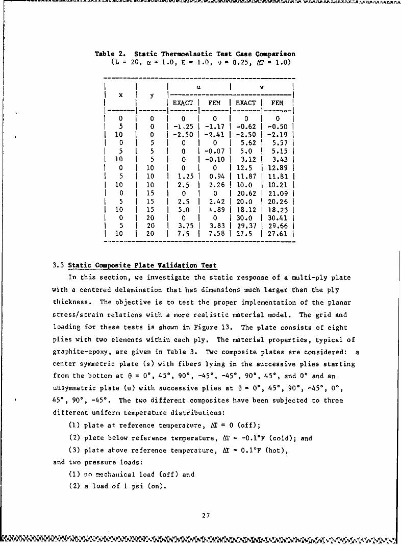
Table 2. Static Thermoelactic Test Case Comparison(L = 20, a = 1.0, E = 1.0, v = 0.25, AT = 1.0)

II I u I vx y ----------------------

EXACT FEM EXACT FEM

0 0 0 0 0 0

5 0 -1,25 -1.17 -0.62 -0.5010 0 -2.50 -q.41 -2.50 -2.19

0 5 0 0 5.62 5.575 5 0 -0.07 15.0 5.15

10 5 0 -0.101 3.12 3.430 I10 0 0 112.5 12.895 I10 1.25 0.94 1 11.87 I11.81

I10 I10 2.5 2.26 i10.0 10.210 15 0 0 20.62 21.095 15 2.5 2.42 20.0 20.26

I10 15 5.0 4.89 18.12 1 18.230 20 0 0 30.0 130.415 20 3.75 3.83 1 29.37 1 29.66

I10 1 20 7.5 7.58 I 27.5 1 27.61

3.3 Static Composite Plate Validation Test

In this section, we investigate the static response of a multi-ply plate

with a centered delamination that has dimensions much larger than the ply

thickness. The objective is to test the proper implementation of the planar

stress/strain relations with a more realistic material model. The grid and

loading for these tests is shown in Figure 13. The plate consists of eight

plies with two elements within each ply. The material properties, typical of

graphite-epoxy, are given in Table 3. Two composite plates are considered: a

center symmetric plate (s) with fibers lying in the successive plies starting

from the bottom at 0 = 00, 450 , 90*, -450 , -450, 900, 450, and 0 and an

unsymmetric plate (u) with successive plies at 0 = 00, 450 90, -45, 00,

450, 90, -45O. The two different composites have been subjected to three

different uniform temperature distributions:

(1) plate at reference temperature, AT = 0 (off);

(2) plate below reference temperature, AT = -0.1*F (cold); and

(3) plate above reference temperature, AT = 0.1 0 F (hot),

and two pressure loads:

(l) no mechanical load (off) and

(2) a load of 1 psi (on).

27

L - 0.25"a - 0.05"b - 0.04"t - 0.005"p a 1 psid - 0.025

ila ----------- w ILL i i

I L

Figure 13. Composite Grid

Table 3. Material Properties Along the Principal Coordinatesof the Fiber Direction

E1 = 1.8x107 psi E2 = E3 = 1.4 x10

6 psi

V12 = V13 = 0.34 V23 0.4 P = 0.055 lb/in 3

G1 2 = G13 = 0.95x106 psi G23 = 0.5x10

6 psi

I al = 2.0xi0-7 (°F) - 1 o2 = a3 = 1.6xi0-5 (OF) - I

The magnitudes of the thermal loads are chosen so that they are approxi-

mately the same magnitude as the pressure loads. Table 4 shows the stress

intensity factors for each ply stacking, pressure, and thermal loading.

It is easy to show that the stress intensity factors behave as a linear

function of the mechanical load and thermal load. A'o, the strain energy

release rate is a quad rat!.. function of the mechanical load and the thermal

luad. The numerical results in Table 4 indicate that the strain energy

release rate shows a strong coupling between the mechanical load and the

thermal load. This implies that the strain energy resulting from a combined

mechanical and thermal load is not simply the sum of the strain energies of

each load independently.

28

I.,%& iA %XJ2 APa. A1~ AP A .&.'A'AU .PZ'. 'US ", . .A TIN N~k I 1'dI A P%._1. PN A I . . I( 'A A A X ".X -_N P A

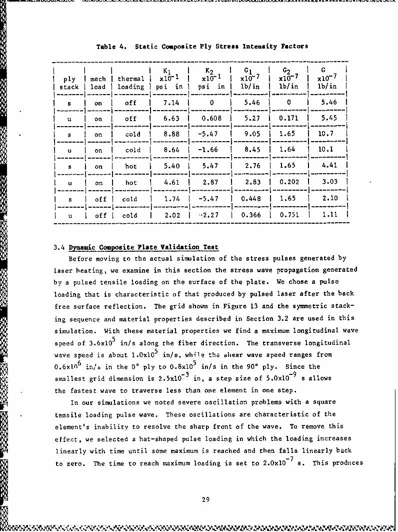
Table 4. Static Composite Ply Stress Intensity Factors

---------------------------------------------------------------------------

I I K I K2 G I 1 ;2 1 ,ply mech I thermal xl0 1- I x0 - I xlO 7 x -10 7 xlO- 7

stack load I loading psi in psi in Ilb/in Ilb/in Ilb/in---------I------------------- ---------- ---------

s on off 7.14 0 5.46 0 5.46

* I--I---------------------- --------- --------- Iu on off 6.63 0.608 5.27 0.171 5.45

....--- I---------------------- -------* s on cold 8.88 -5.47 9.05 1.65 I10.7

------ - -- -- - - - -- - -- - -- - - - -- - - - -- -- --u I on cold 8.64 -1.66 8.45 1.64 i10.1I

I-- ---.--------- -------- ----- -------s on hot 5.40 5.47 2.76 1.65 4.41

------I--I----- ----------------- --------- --------- Iu on hot 4.61 2.87 2.83 0.202 3.03

.....- I--------- ------ I------- -------s off cold 1.74 -5.47 0.448 1.65 2.10

--------------- ---------------- ------u off cold 2.02 I-2.27 0.366 I 0.751 I1.11I

------------------------------------------------------------------

3.4 Dynamic Composite Plate Validation Test

Before moving to the actual simulation of the stress pulses generated by

laser heating, we examine in this section the stress wave propagation generated

by a pulsed tensile loading on the surface of the plate. We chose a pulse

loading that is characteristic of that produced by pulsed laser after the back

free surface reflection. The grid shown in Figure 13 and the symmetric stack-

ing sequence and material properties described in Section 3.2 are used in this

simulation. With these material properties we find a maximum longitudinal wave

speed of 3.6xi05 in/s along the fiber direction. The transverse longitudinal

wave speed is about l.Oxl05 in/s, while the ehear wave speed ranges from

0.6xlN 6 in/ in the 0 ° ply to 0.8xlO 5 in/s in the 900 ply. Since the

smallest grid dimension is 2.5x107 3 in, a step size of 5.0xlO- 9 s allows

the fastest wave to traverse less than one element in one step.

In our simulations we noted severe oscillation problems with a square

tensile loading pulse wave. These oscillations are characteristic of the

element's inability to resolve the sharp front of the wave. To remove this

effect, we selected a hat-shaped pulse loading in which the loading increases

linearly with time until some maximum is reached and then falls linearly back

to zero. The time to reach maximum loading is set to 2.OxlO s. This produces

29

a stress wave within the body that rises and falls within eight elements or

four ply widths, and the oscillations are only modest. Ratios of half-

wavelength to element size smaller than four show marked oscillations

regardless of the step size using the Newmark method. The Wilson method with

its inherent numerical damping proved to be only a slightly better option,

since little damping was apparent fcr small time step sizes and too much

damping or loss in accuracy was observed for the larger step sizes. These

wave resolving restrictio.s have some important implications especially for

sharp laser pulses in three-dimensional simulations, which we discuss further

in Section 6.

In Figures 14 through 23, we show the qtress contours at different times

for the simulation of the symmetric plate. These contours are plotted on the

exaggerated deformed geometry. Since the tensile load at a maximum of l.0xl0 6

psi is applied uniformly across the top surface, the stress wave is very

uniform before it interacts with the delamination. In Figure 14, we see the

normal transverse wave at a time just before its head reaches the delamination

and before the end of the boundary loading pulse. Note that the delamination

(marked by the line ending with the asterisk) is assumed closed initially.

Although the delamination is initially in the center, the tensile deformation

in the wave has stretched the top plies in this exaggerated plot. In

Figure 15, the transverse normal stress is shown as the maximum stress passes

in front of the crack. We see that the delamination has opened almost

uniformly across its length. Also, we see the first signs of a compression

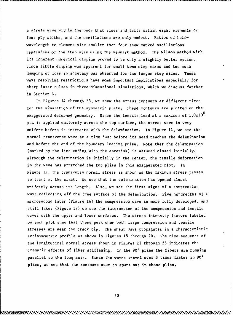
wave reflecting off the free surface of the delamination. Five hundredths of a

microsecond later (Figure 16) the compression wave is more fully developed, and

still later (Figure 17) we see the interaction of the compression and tensile

waves with the upper and lower surfaces. The stress intensity factors labeled

on each plot show that these peak when both large compression and tensile

stresses are near the crack tip. The shear wave propagates in a characteristic

antisymmetric profile as shown in Figures 18 through 20. The time sequence of

the longitudinal normal stress shown in Figures 21 through 23 indicates the

dramatic effects of fiber stiffening. In the 90* plies the fibers are running

parallel to the long axis. Since the waves travel over 3 times faster in 90*

plies, we see that the contours seem to spurt out in these plies.

30

X'AKQ -19 7Pdip r'J\JY

LOACCAVE V 13 TESTEP 15 TIME: 0.00000015FRANE OF RWi SLOBA.STRIESS Y HIMW -3.17E*03 IMAXL 1.61E14 4-.8

7.0-3.

7.0

1.0

-9.00E4LEVEI.. D0ELTA: Z.OOE+04 S.00EWV4

Figure 14. Normal Stress (t - 0.15 us)

LOAOCASE 30 TIMESTEP~30 TIME: 0.0000003FRAME OF REF: GLOBALSTRESS - Y MIA: -2.26140 MAX, 1.001405 K 841

X2 - -3.1 I101

1.0

-9.0E404LEVELS: 10 DELTA:~ Z.00(404 9.90Ef"

Figure 15. Normal Stress (t -0.3 Ua)

31

LOADCASE:35 TIMESTEP:35 TME: 0.000000.5FRAME OF iEF. GLOSAL 3

STRESS - M 8I.-a.05E:.04 ".AX: 8.41E+04 I- 8.7 10

K2 - -2.2 x 10

7.0 ,

-B.00E+04 LEVELS: 10 DELTA: 2.00E*04 S. COEV"

Figure 16. Normal Stress (t = 0.35 Vx)

LOADCASE: 40 T7IESTEP. 40 TIME: 0.0000004FRAME OF REF: GLOBALSTRESS - Y MIN:-S.89E+04 MAX: 0.98E404 K I 6.6 103

K2 - 8.2

-9.OOE+04 LEVELS: 10 DELTA: 2.OOE+04 .OOEF-

Figure 17. Normal Stress (t 0.4 us)

32

LOADCASE 30 TIMESTEP. 30 TIME:~ 0.000003FRAME OF REP LOBAL,STRESS - XY 141k -2.43E*04 M4AX: 2.36E*04

-0.3

0.3

-W.70E+94 LEVELS: 10 DELTA: 6. WE+03 2.70EV"

Figure 18. Shear Stress (t -0.3 lie)

LOADCASE: 35 TIMESTEP 35 TIME; 0.00000035FRAME OF REF: BLOO..STRESS - XY HMN:-3.72E+04 MAX: 3.57E*04

-2.70E+04 LEVELS: 10 DELTA: §.OOE+03 2.70EU"

Figure 19. Shear Stress (t *0.35 us)

33

LOADCASE: 40 TIMESTEP: 40 TIME: 0.0000004FRAME OF REF: GLOBALSTRESS - XY MIN:-3.0BE+04 MAX: 3.04E+04

Y

Figure 20. Shear Stress (t = 0.4 i')

LOAOCASE: 30 TIMESTEP: 30 TIME: 0.0000003FRAME OF REF: GLOBALSTRFESS - X M1"N: -4.59E+04 MA)X: 3.48E+C4

- 0.5

0.3

!V

-4.50E+04 LEVELS:10 DELTA: 1.OOE.04 4.70EU4U

Figure 21. Longitudinal Shorml Stres (t = 0.3 is)

34

KAM X ~~ k

LOADCASE:35 TIMESTEP:35 TIME: 0.00000035FRAME OF REF: GLOBALSTRESS - X MIN:-4.11E+04 MAX: 4.57E+04

I35-.

-4.50E+04 LEVELS: 10 DELTA: 1.00E*04 4 .50EDM

* Figure 22. longitudinal Normal Stress (t *0.35 118)

LOAOCASE: 40 TIMESTEP.40 TIME: 0.0000004FRAME OF REF: GLOCALSTRESS - X MIN: -3.55E+04 MAX; 3.73E+04

3.5

2.5

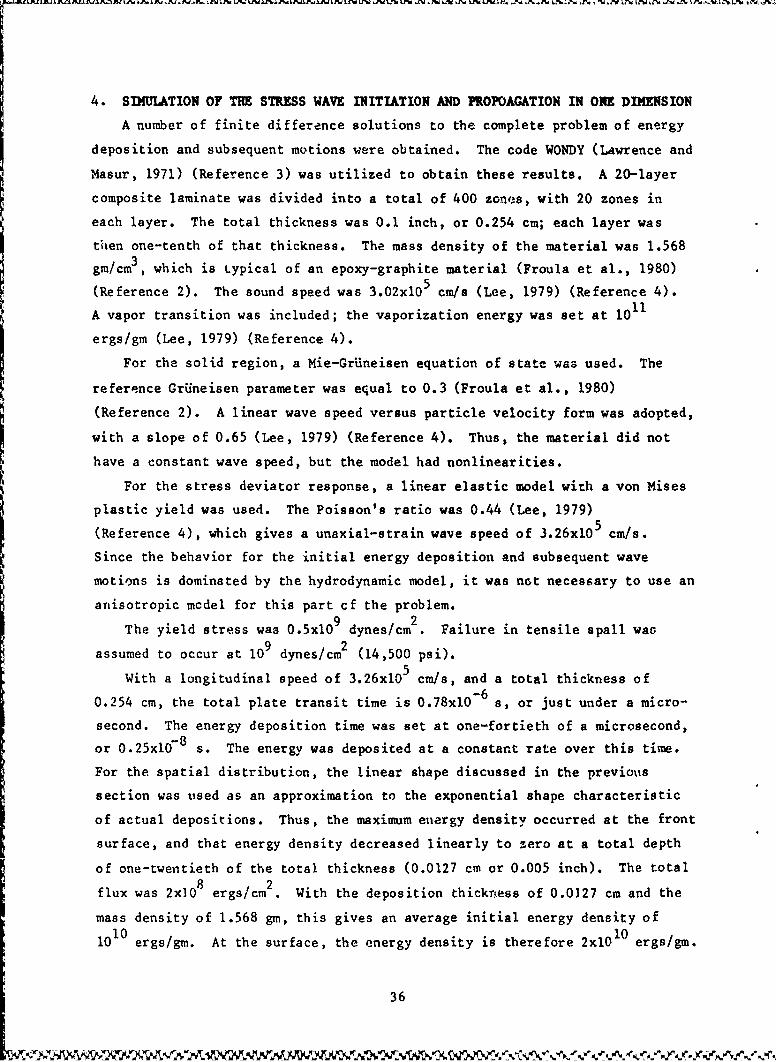
4. SIMULATION OF THE STRESS WAVE INITIATION AND PROPOAGATION IN ONE DIMENSION

A number of finite difference solutions to the complete problem of energy

deposition and subsequent motions were obtained. The code WONDY (Lawrence and

Masur, 1971) (Reference 3) was utilized to obtain these results. A 20-layer

composite laminate was divided into a total of 400 zones, with 20 zones in

each layer. The total thickness was 0.1 inch, or 0.254 cm; each layer was

then one-tenth of that thickness. The mass density of the material was 1.568

gm/cm3 , which is typical of an epoxy-graphite material (Froula et al., 1980)

(Reference 2). The sound speed was 3.02xi05 cm/s (Lee, 1979) (Reference 4).

A vapor transition was included; the vaporization energy was set at 1011

ergs/gm (Lee, 1979) (Reference 4).

For the solid region, a Mie-GrUneisen equation of state was used. The

reference GrUneisen parameter was equal to 0.3 (Froula et al., 1980)

(Reference 2). A linear wave speed versus particle velocity form was adopted,

with a slope of 0.65 (Lee, 1979) (Reference 4). Thus, the material did not

have a constant wave speed, but the model had nonlinearities.

For the stress deviator response, a linear elastic model with a von Mises

plastic yield was used. The Poisson's ratio was 0.44 (Lee, 1979)

(Reference 4), which gives a unaxial-strain wave speed of 3.26xi0 5 cm/s.

Since the behavior for the initial energy deposition and subsequent wave

motions is dominated by the hydrodynamic model, it was not necessary to use an

anisotropic mcdel for this part cf the problem.9 2

The yield stress was 0.5xlO dynes/cm . Failure in tensile spall was

assumed to occur at 109 dynes/cm2 (14,500 psi).

With a longitudinal speed of 3.26xi05 cm/s, and a total thickness of

0.254 cm, the total plate transit time is 0.78xi0 - 6 s, or just under a micro-

second. The energy deposition time was set at one-fortieth of a microsecond,

or 0.25x1078 s. The energy was deposited at a constant rate over this time.

For the spatial distribution, the linear shape discussed in the previous

section was used as an approximation to the exponential shape characteristic

of actual depositions. Thus, the maximum energy density occurred at the front

surface, and that energy density decreased linearly to zero at a total depth

of one-twentieth of the total thickness (0.0127 cm or 0.005 inch). The total8 2

flux was 2x1O ergs/cm . With the deposition thickness of 0.0327 cm and the

mass density of 1.568 gin, this gives an average initial energy density of

1010 ergs/gm. At the surface, the energy density is therefore 2x10 ergs/gm.

36

Since the GrUneisen is 0.3, an instantaneous deposition of this energy would

create an initial stress of P = (1.568)(0.3)(2xlO 0) = 9.5xlO9 dynes/cm 2 , or

just under 10 kilobars, with a pulse width of 0.0127 cm. In fact, because of

the finite deposition time, the actual pulse width is slightly higher, and the

initial stress about half that value.

As discussed in Section 1.3, an initial triangular compressive pulse will

generate a tensile following "tail" as it moves away from the free surface.

As that tail builds in magnitude, tensile spall of the front surface will

occur. Additional spall will occur until the final tensile magnitude decreased

to under the spall strength of I kilobar.

Figure 24 shows the actual resultant wave at the time of 10- 7 s, well

after the final wave has moved away from the free front surface. The main

compressive pulse is about 3 kilobars (40xlO3 psi) at this time and is

indeed almost triangular in shape. At times immediately after the energy

deposition, parts of the front surface did spall as the tensile wave began to

grow. Ultimately, a total thickness one-half the deposition depth was spalled.

The tensile following wave, which was almost a kilobar at the time of final

spall, has at this time decreased to about two-thirds of a kilobar.

This result illustrateL the important effects of the material

nonlinearities and especially the effects of the spall resporise. It is 4. j

worthwhile noting that, in this particular problem, the initial energy

densities were below the vaporization energy (10 1 ergs/gm) by a factor of 5.

If the energy flux had been greater, the material near the free surface would

have been vaporized, and the tensile strength would have decreased to zero.

The wave shown in Figure 24 propagates into the interior of the plate.

Since the material is nonlinear, the stress pulse will decay in magnitude and

broaden in width. For example, Figure 25 shows the resultant wave at the time

of 0.7x10- 6 s, just before it reaches the back free surface of the plate.

At this time, the peak compressive wave has decayed to 30,000 psi, and the

tensile portion has decayed to less than 6000 psi. The pulse is almost twice

as wide as it was initially.

37

INITIAL FULLY DEVELOPED WAVESTRESS (PSI)

10145.0 .. . . .

0.0

-0000.0 -

-20000.0-

- SPALL

-30000.0

-38462.0 " - * - ,'0.0 S.OE-03 I.OE-02 1.5E-02 2.1E-02

Distance

Figure 24. Initial Fully Developed Stress Wave (t = 0.1 ps)

WAVE JUST BEFORE FREE SURFACE REFLECTIONSTRESS (PSI)

5762.0 ' ' '

0.0 ___-

10000.0

reSS

-20000.0

-30044.00.0 4.OE-02 S.OE-02 I.OE-01

ODitance

Figure 25. Stress Wave Just Before Free Surface Reflection (t - 0.7 Us)

38

5. SIMULATION OF THE STRESS WAVE INTERACTION WITH A DELAMINATION

As the stress wave reflects from the wall one would expect the surface

plies to spall. To simulate such an event, we model the four plies adjacent to

the surface. In the middle of these four plies is a small delamination with a

half-length of 0.025 inch. The grid is the same as that used in the previous

composite simulations (Figure 13), but the dimensions are reduced by half to

give four elements per ply. The initial conditions are taken from the one-

dimensional simulation at a time just before the reflection of the wave but

just after the compressive part of the wave passes the delamination. The top

and bottom surfaces are both considered stress-free. Since the stress wave

lies ithin about two plies, the bottom surface observes essentially no stress

from the time the compressive wave passes over until the time the reflected

tensile wave returns. It is during this time frame that we have conducted a

series of simulations varying the ply stacking sequence, plate temperature,

crack geometry, and boundary restraints. Table 5 gives a summary of the test

cases and the maximum fracture intensity values observed over each simulation.

In the first six cases we vary the stacking sequence and observe that the

maximum fracture parameters vary little from case to case. Even though the

loading is not symmetric, the plates with delaminations between similiar plies

sho ... ..odc I eff. cts. Plate- .... el. - fto ions between dissimilar plies

show a small mode II effect, but still it is minor compared to a mode I

fracture. The mode II strain energy release rate is especially small because

the differential in the deformation tangent to the crack is small. Since the

mode I strain energy release rate is defined primarily by the Young's modulus

of the matrix, this parameter varies little with the ply sequence.

Wang et al. (1980) (Reference 12) found that, since the curing temperatures

are so high (300F), the thermal stress at room temperature is an important

consideration when evaluating the strain energy release rate. To test this

effect, in case 7, the plate is assumed to be 200*F colder than the reference

temperature. In comparison to case I, a significant change in the strain

energy release rate is seen, indicating that the ambient temperature of the

plate plays an important role in defining its fracture resistance. In this

simulation, we assumed that the temperature of the plate suddenly dropped

200*F. This may give rise to some unwanted dynamical effects near the

constrained regions of the plate. Since the delamination is removed from

39

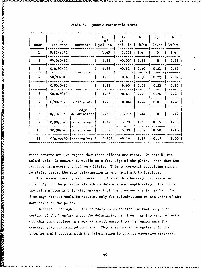
Table 5. Dynamic Parametric Tests

I I K1 K2 G1 G2 Gply I I x103 x103

case sequence comments psi in I psi in I b/in I b/in I b/in I---------------------------------------------

1 0/90/90/0 1.65 0.009 2.4 0 2.44---------------------------------------------------- ------- I

2 90/0/0/90 1.28 -0.004 2.31 0 2.31

-------------------------------------------------- -------I3 0/0/90/90 1.36 -0.62 2.40 0.23 2.42

--- ------------------------------------------- ----------4 90/90/0/0 1.33 0.61 2.30 0.22 2.32

-------------------------------------------------- -------I5 0/90/0/90 1.33 0.60 2.29 0.25 2.32

-------------------------------------------------- -------6 90/0/90/0 1.36 -0.61 2.40 0.26 2.43

-------------------------------------------------- -------I7 0/90/90/0 cold plate 1.23 -0.062 1.44 0.01 1.45

-------------------------------------------------- -------Iedge

1 8 1 0/90/90/9 Idelaminationl 1.65 1 -0.015 1 2.44 1 0 1 2.44 1------ I--------I---------I-------I-------I-----I-----I-----I1 9 1 0/90/90/0 Iconstrained 1 1.24 1-0.73 1 1.38 1 0.15 1 1.53 1

------- I--------- I----------I -------- I -------- I ------ I ------I ------ Ii10 1 90/90/0/0 Iconstrained 1 0.998 1 -0.33 1 0.92 1 0.50 1 1.13 1

------- I--------- I----------I -------- I -------- I ------I ------I ------ II11 0/0/90/90 Irnn. frai ned I n797 -0.10 I 1.38 1 0.17 1.55 1

these constraints, we expect that these effects are minor. In case 8, the

delamination is assumed to reside on a free edge of the plate. Note that the

fracture parameters changed very little. This is somewhat surprising since,

in static tests, the edge delamination is much more apt to fracture.

The reason these dynamic tests do not show this behavior can again be

attributed to the pulse wavelength to delamination length ratio. The tip of

the delamination is initially unaware that the free surface is nearby. The

free edge effects would be apparent only for delaminations on the order of the

wavelength of the pulse.

In cases 9 through 11, the boundary is constrained so that only that

portion of the boundary above the delamination is free. As the wave reflects

off this back surface, a shear wave will ensue from the region near the

constrained/unconstrained boundary. This shear wave propagates into the

interior and interacts with the delamination to produce excessive stresses.

40

Since the shear wave is partially transmitted via the fibers, one would expect

to see variations in the fracture parameters depending on the stacking

sequence. The tests conducted verify this sensitivity. Since the shear waves

travel slowcr than the normal stress waves, the maximum value of the mode II

fracture parameters peak at a later time than the mode I parameters.

In all the simulations, the maximum fracture intensity conditions occurred

after the maximum of the tensile stress wave had passed slightly beloD the

crack and the compressive wave had partially reflected from the crack f'ee

surface. The critical strain energy release rate for unstable growth is still

in question, but under static loading tests Wang et al. (1980) (Reference 12)

quoted a value of 0.8 lb/in. This would imply that the spalling occurs well

before the maximum intensity conditions at a time just before the maximum

stress reaches the crack. In such a scenario, most of the energy would remain

as kinetic energy in a spall the size of which would be related to the stress

wavelength. This would effectively damp the wave in the main body by

preventing this energy from being converted to strain energy. The spall would

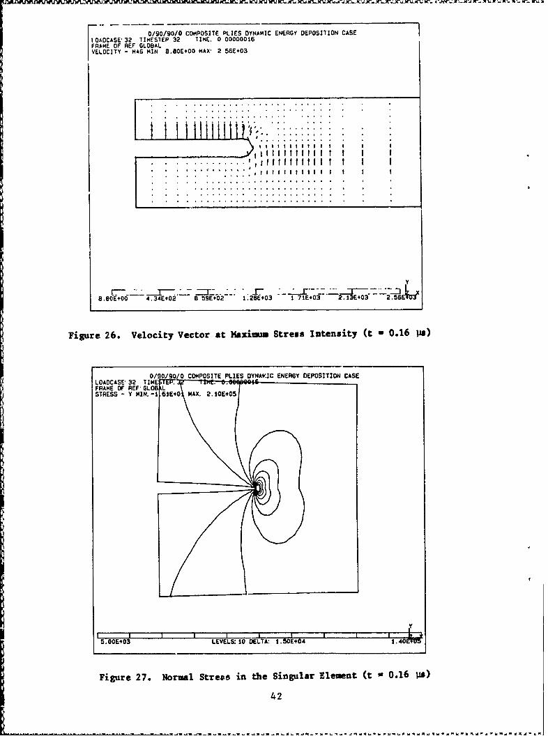
travel at a high rate of speed away from the main body. The velocity vector

plot in Figure 26 shows speeds on the order of 150 mph at the time of maximum

fracture intensity.

None of the simulations indicate that the initial tensile tail plays much

of a role in the fracture of the composite. This may not be true for loading

conditions other than the magnitude and profile assumed in the one-dimensional

simulations in Section 4.

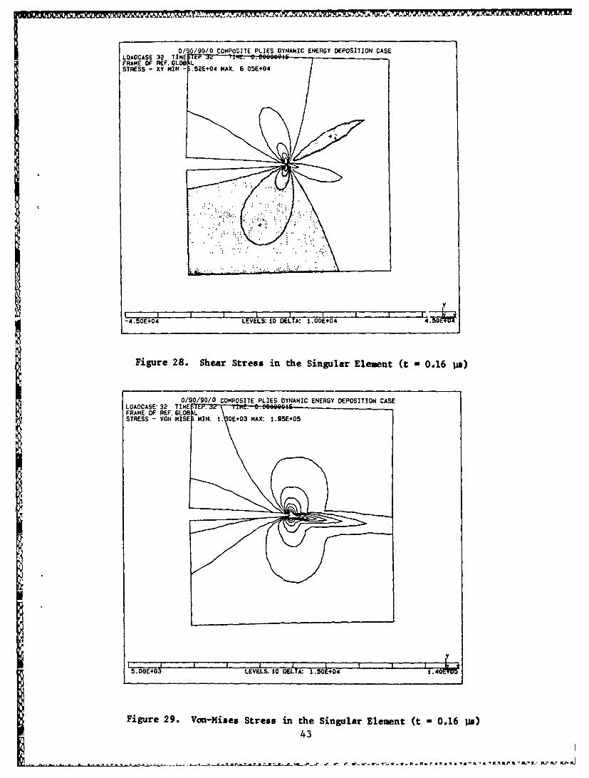
Plots of the transverse normal and shear stress contours within the

singular element (0.0025 inch on edge) given in Figures 27 and 28 show a very

typical pattern. These plots are at a time of maximum fracture intensity. As

the wave interacts with the delamination, the region near the crack tip could

behave plastically. With this in mind, the contours of von Mises stress

plotted in Figure 29 give an indication of the size of the plastic region.

41

0/90/90/0 COMPOSITE PLIES DYNAMIC ENERGY DEPOSITION CASEOADCASE 32 IIMESIEP 32 TIME. 0 00000016

FRAME OF REF GLOBALVELOCITY - NAG MIN 8.80E+00 MAX* 2 56E+03

......... .) ' i i i i i ..

. . ..... ..... I I:,,tt I I,i •, . . . f lt lll tt I I

. . .. . . . . . . . . . . .

........................................................ ,,,,,

. . . ... ... . .. .. . . .

! Y

8.SOE+00 4.34E+02 8 59E+02 1.28E403 1 71E+03 2.13E 03 2.56E

Figure 26. Velocity Vector at Maximum Stress Intensity (t = 0.16 ps)

0/90/90/0 COMPOSITE PLIES DYNAMIC ENERGY DEPOSITION CASELOADCASE' 32 TIME P. . .FRAME OF REF' GLOBkLSTRESS - Y MIN. - .61EO MAX. 2.IOE05

Y

5.0E$I03 LEVELS: 10 DELTA: 1.50E+04 I,4o11.4

Figure 27. Normal Stresa in the Singular Element (t - 0.16 ps)

42

v ~ ~ ~ ~ & VW I MU~ wU W.xD7TM37&W1v)v- - - - -

D/90/90/0 COMPOSI7E PLIES DYNAMIC ENERGY DEPOSITION CASE77~LOADCASE 32 TIMET dFRAME OF REF. GLOB LSTRESS -XY MIN -i. 52E+Od MAX. 6 05E+4

Y

-4.50E+04 LEVELS:10 DELTA: I.ODE4 4730e

Figure 28. Shear Stress in the Singular Element (t 0.16 usa)

0/90/90/0 COMPOSITE PLIES DYNAMIC ENERGY DEPOSITION CASELOACCASE*32 TIMEFRAME OF REF. GLOBkLSTRESS - VON MISE MIN. 1. OEt03 MAX: 1.95E+05

5.OOE+03 LEVELS. 10 DELTA: 1.50E+04 1.40eD5m

Figure 29. Von-Mises Stress in the Singular Element (t a 0.16 ps)

43

1 - . -- t- -1. - . . .a .- -5 ft -' ft' S .IL r J r

6. UNIFIED MODEL FEASIBILITY STUDY

The long-range goal of this study is the development of a complete finite

element program for rapid thermal loading that is capable of an accurate and

complete thermodynamic description similar to the finite difference code used

in this study. As an interim measure we have used the finite difference model

to describe the energy deposition aspects of the problem and to follow the

resulting waves until they decay into the lower temperature solid behavior.

At this level, a transfer to the finite element code is made to study the sub-

sequent interaction with a pre-existing delamination. Such a treatment cannot,

however, properly treat the coupling of the effects of the crack on the stress

wave generation, which could be important for delaminations near the irradiated

surface. In addition to these coupling effects, each of the individual models

used in this Phase I study are inadequate, in certain respects, for describing

the high-energy, high-stress behavior of the composite material. This is in

part due to the lack of experimental data related to composites in this regime.

Nevertheless, certain aspects could be improved with current knowledge. For

example, in the current finite element model, the composite is treated as a

linearly elastic anisotropic material. Certainly, as the plate is heated, an

epoxy matrix would undergo some phase transition that alters its elastic

properties, while the graphite fibers might retain their elastic properties at

the same temperature. The result would be some anisotropic medium that behaves

like a fluid in certain directions. Similarly, after the wave has moved out

of the high-temperature region, the high stresses might cause the matrix to

deform plastically.

Certain algorithmic features need to be employed to allow for more than

one delamination, create new delaminations, and allow for partial or full

closing of delaminations depending on the nature of the stress wave. The logic

for closing delaminations may be conveniently expressed in the finite element

context via Lagrangian multipliers. These multipliers represent the contact

force between the sides of the delamination. In addition to interlaminar

delaminations, the model should consider transverse cracks, which may be

important when normal operating loads are also considered in the analysis.

In the current work, the stress wave generation was carried out in one

dimension. This limits the analysis to the generation of longitudinal waves.

The next step would be to carry out the analysis in two dimensions under plane

stress/strain or axisymmetric assumptions. Strictly speaking, the anisotropic

44

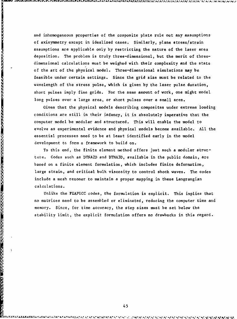
and inhomogeneous properties of the ccinposite plate rule out any assumptions

of axisymmetry except in idealized cases. Similarly, plane stress/strain

assumptions are applicable only by restricting the nature of the laser areadeposition. The problem is truly three-dimensional, but the merit of three-

dimensional calculations must be weighed with their complexity and the state

of the art of the physical model. Three-dimensional simulations may be

feasible under certain settings. Since the grid size must be related to the

wavelength of the stress pulse, which is given by the laser pulse duration,

* short pulses imply fine grids. For the same amount of work, one might model

long pulses over a large area, or short pulses over a small area.

Given that the physical models describing composites under extreme loading

conditions are still in their infancy, it is absolutely imperative that the

computer model be modular and structured. This will enable the model to

evolve as experimental evidence and physical models become available. All the

essential processes need to be at least identified early in the model

development tc form a framework to build on.

To this end, the finite element method offers just such a modular struc-

ture. Codes such as DYNA2D and DYNA3D, available in the public domain, are

based on a finite element formulation, which includes finite deformation,

large strain, and critical bulk viscosity to control shock waves. The codes

include a mesh rezoner to maintain a proper mapping in these Langrangian

calculations.

Unlike the FEAPICC codes, the formulation is explicit. This implies that

no matrices need to be assembled or eliminated, reducing the computer time and

memory. Since, for time accuracy, the step sizes must be set below the

stability limit, the explicit formulation offers no drawbacks in this regard.

I .:' ! M A 1'9 I, ?"M I A hA . A .- X' 'A ~ #' 11 4.'~ C' 5C '' ~ .'I"~7 C ''PN. 'C 'P '.'. 2 7P'C '

7. •ONCLUSIONS

To summarize, we have addressed the problem of rapid deposition of thermal

energy on the surface of a composite plate. Several general aspects of the

problem have been described, and the assumptions regarding the analysis have

been enumerated. Existing codes have been modified to solve the stress pulse

generation and its subsequent interaction with a delamination within the

composite plate. The finite difference model for simulation of the stress

wave generation includes the thermomechanical coupling and a general equation

of state model to account for phase changes. The finite element model accounts

for the stress singularity of a delamination within the anisotropic composite

plies. This model has been modified to include thermal stresses, to calculate

the strain energy release rates, and to account properly for the plane strain

assumptions. Tests have been conducted to ensure that the modifications have

been implemented correctly and that the model is applicable to the problem we

address.

Our analysis shows that the strain energy is a quadratic function of the

mechanical and thermal loading with a strong coupling between the mechanical

and thermal parts. While the study of Wang et al. (1980) (Reference 12)

implies the contrary, the strain energy resulting from a combined mechanical

and thermal load is not generally the sum of the strain energies of each load

independently.

The results of the analysis of the stress wave generation indicate that

the ensuing wave will have both compressive and tensile parts. The magnitude

of the tensile part depends on the tensile strength or fracture toughness of

the surface plies. As the wave propagates into the interior cf the plate, the

nonlinearities damp and spread this wave.

We have modeled, using the singular finite element method, the spalling

event as the stress wave reflects from the back surface and interacts with an

existing delamination. Our analysis indicates that the fracture parameters are

insensitive to the stacking sequence when the delamination interacts with a

pure tension wave. This is because the stress is transmitted primarily through

the matrix. If a shear wave results from the loading or boundary constraints,

then th-e stacking sequence has an appreciable effect on the fracture param-

eters, since the shear wave is transmitted via the fiber/matrix combination.

The ambient temperature of the plate also proved to be an important considera-

tion in the fracture, since the thermal deformation resulting from the curing

of the composite can be significant.

46

X, NI ?%.,I .Vk L xA K- .1 1 p ,- - .- 0 W J4 4j X ".1 PJ M A A.~ -LA. j -.A A, 1P. M i, e' r

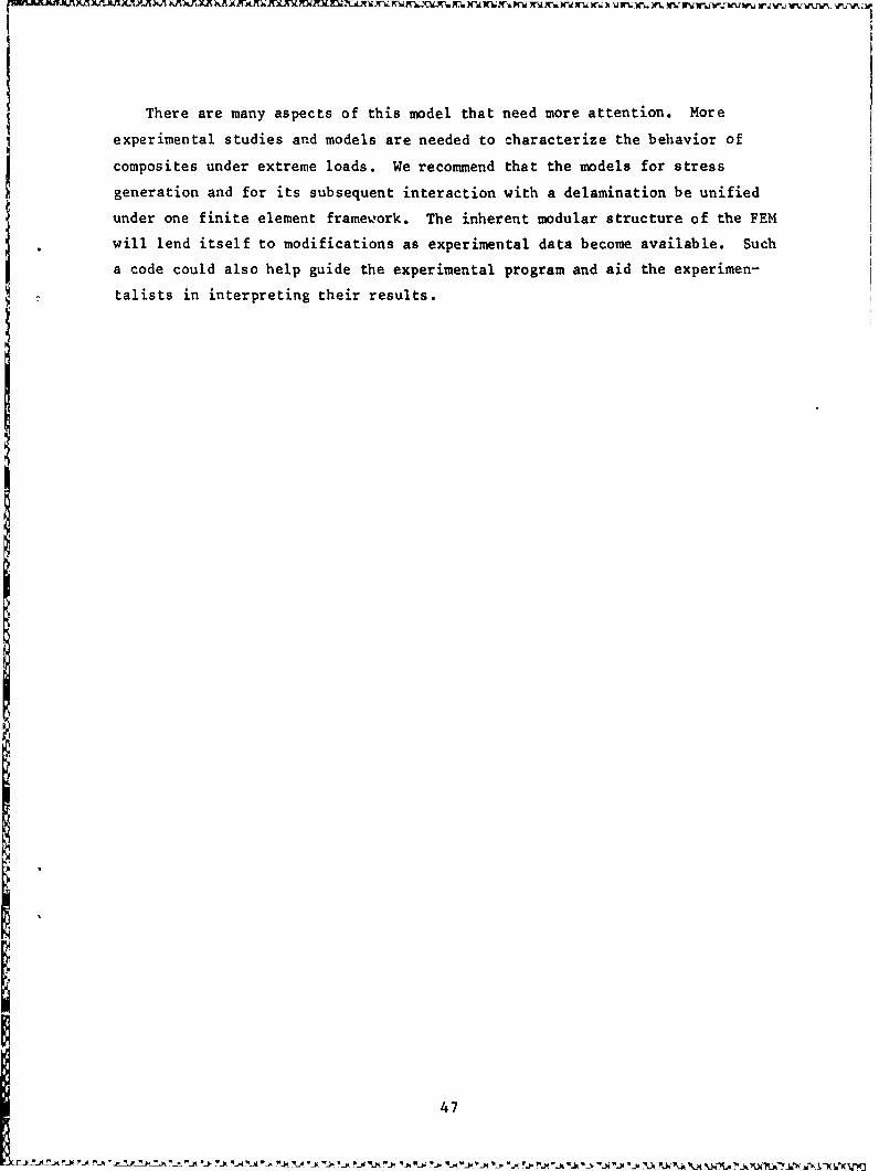
There are many aspects of this model that need more attention. More

experimental studies and models are needed to characterize the behavior of

composites under extreme loads. We recommend that the models for stress

generation and for its subsequent interaction with a delamination be unified

under one finite element framework. The inherent modular structure of the FEM

will lend itself to modifications as experimental data become available. Such

a code could also help guide the experimental program and aid the experimen-

talists in interpreting their results.

47

IJ47

REFERENCES

1. Aminpour, M. A. (1986) "linite Element Analysis of Propagating InterfaceCracks in Composites," Ph.D. Thesis, University of Washington, Dept. ofAeronautics and Astronautics.

2. Froula, N. H., Leikes, G. L., Stretanski, E. D., and Swick, M. K. (1980)"Grtneisen Parameter Measurements for Kevlar and Epoxy," Air ForceWeapons Laboratory Report AFWL-TR-79-176, August.

3. Lawrence, R. J., and Masur, D. S. (1971) "Wondy IV - A Computer Program forOne-Dimensional Wave Propagation with Rezoning," Sandia Laboratories

Report SC-RR-71028, August.

4. Lee, L. M. (1979) "Graphite Resin Characterization Program for NuclearHardness Evaluation," Air Force Weapons Laboratcry ReportAFWL-TR-79-103.

5. Lin, K. Y., and Mar, J. W. (1976) "Finite Element Analysis of StressIntensity Factors for Cracks at a Bi-material Interface," Int. J. ofFracture, Vol. 12, No. 4, August, pp. 521-531.

6. O'Leary, J. R. (1981) "An Error Analysis for Singular Finite Elements,"TICOM Report 81-4, August.

7. Paramasivam, T., and Reismann, H. (1986) "Laser-Induced Thickness Stretch

Motion of a Transversely Constrained Irradiated Slab," AIAA J., Vol.24, No. 10, October, pp. 1650-55.

8. Rice, J. R., and Sih, G. C. (1965) "Plane Problems of Cracks in DissimilarMedia," J. Appl. Mech., June, pp. 418-423.

9. Stern, M. (1979) "Families of Consistent Conforming Elements with SingularDerivative Fields," Int. J. Num. Meth. in Eng., Vol. 14, pp. 409-421.

10. Tong, P., Pian, T. H. H., and Lasry, S. (1973) "A Hybrid Element Approachto Crack Problems in Plane Elasticity," Int. J. Num. Meth. in Eng.,Vol. 7, pp. 297-308.

S11. Walker, T., and Lin, K. Y. (1987) "A Singular Finite-Element Analysis ofInterface Fracture in Composite Material," to be published.

12. Wang, A. S. D., Crossman, F. W., Law, G. E., and Warren, J. (1980) "AComprehensive Study of Interlaminar and Intralaminar Fracture Growth in

Composite Laminates," Annual Technical Report co AFOSR for ContractNo. F49620-79-C-0206, Drexel University, November.

48