Embed Size (px)
Citation preview

Study on the Modelling of Airport Economic Value
Final Report
November 2016

Background information This report presents the final status of the study on modelling Airport Economic Value. This study was commissioned by the Airport Research Unit of EUROCONTROL to the University of Westminster supported by Innaxis as part of its contribution to SESAR Operational Focus Area (OFA) 05.01.01 entitled ‘Airport Operations Management’, in relation to the development of the AirPort Operations Centre (APOC) concept. The objective of the study is to extrapolate the model used for capacity planning of en-route ACC centres to airports with a view to evaluate the optimum airport economic value, based on several cost functions and quality of service evaluations. For any questions on the content of this report, please contact us at: [email protected] [email protected] Authorship Gérald Gurtner, Andrew Cook, Anne Graham – University of Westminster (London) Samuel Cristóbal – Innaxis (Madrid)

Contents
1 Introduction and objectives 11
2 Literature and data availability reviews 132.1 Literature review . . . . . . . . . . . . . . . . . . . . . . . . . . . . . . 13
2.1.1 The implications of airport congestion and delays . . . . . . . . 132.1.2 Soft management options . . . . . . . . . . . . . . . . . . . . . . 142.1.3 Hard infrastructure approaches . . . . . . . . . . . . . . . . . . 15
2.2 Data availability . . . . . . . . . . . . . . . . . . . . . . . . . . . . . . 17
3 Model preparation and calibration 203.1 Preparing for the modelling process . . . . . . . . . . . . . . . . . . . . 20
3.1.1 Using the literature review . . . . . . . . . . . . . . . . . . . . . 203.1.2 Using the data analysis . . . . . . . . . . . . . . . . . . . . . . . 21
3.2 High-level principles of the modelling process . . . . . . . . . . . . . . . 293.3 Calibration . . . . . . . . . . . . . . . . . . . . . . . . . . . . . . . . . 31
3.3.1 Functional relationships . . . . . . . . . . . . . . . . . . . . . . 323.3.2 Direct calibration of parameters . . . . . . . . . . . . . . . . . . 333.3.3 Post-calibration of parameters . . . . . . . . . . . . . . . . . . . 34
4 Model implementation and results 364.1 Implementation . . . . . . . . . . . . . . . . . . . . . . . . . . . . . . . 36
4.1.1 Engine implementation . . . . . . . . . . . . . . . . . . . . . . . 364.1.2 Graphical user interface (GUI) . . . . . . . . . . . . . . . . . . . 36
4.2 Calibrated model results . . . . . . . . . . . . . . . . . . . . . . . . . . 384.2.1 Calibrated airport . . . . . . . . . . . . . . . . . . . . . . . . . . 384.2.2 Comparing different airports . . . . . . . . . . . . . . . . . . . . 404.2.3 Effect of parameters on the position of the optimum . . . . . . . 42
4.3 Exploratory results . . . . . . . . . . . . . . . . . . . . . . . . . . . . . 464.3.1 ‘Better shopping time’ . . . . . . . . . . . . . . . . . . . . . . . 474.3.2 ‘Longer shopping time’ . . . . . . . . . . . . . . . . . . . . . . . 474.3.3 Both effects . . . . . . . . . . . . . . . . . . . . . . . . . . . . . 48
5 Conclusions 50
3

Airport Economic Value D1.2
A Data analysis 54A.1 Correlation structure . . . . . . . . . . . . . . . . . . . . . . . . . . . . 54A.2 Clustering analysis . . . . . . . . . . . . . . . . . . . . . . . . . . . . . 61
A.2.1 Methodology . . . . . . . . . . . . . . . . . . . . . . . . . . . . 61A.2.2 Analysis of clusters . . . . . . . . . . . . . . . . . . . . . . . . . 62
B The model 65B.1 Calibration . . . . . . . . . . . . . . . . . . . . . . . . . . . . . . . . . 65
B.1.1 The problem of delay . . . . . . . . . . . . . . . . . . . . . . . . 65B.1.2 Delay and capacity . . . . . . . . . . . . . . . . . . . . . . . . . 65B.1.3 Cost of delay . . . . . . . . . . . . . . . . . . . . . . . . . . . . 67
B.2 Model implementation . . . . . . . . . . . . . . . . . . . . . . . . . . . 69B.2.1 Probability of operation . . . . . . . . . . . . . . . . . . . . . . 69B.2.2 Implicit equation of delay . . . . . . . . . . . . . . . . . . . . . 71B.2.3 The airport . . . . . . . . . . . . . . . . . . . . . . . . . . . . . 71
B.3 Exploratory analysis . . . . . . . . . . . . . . . . . . . . . . . . . . . . 72
C Sensitivity analysis 74
4

List of Figures
1 Maximum of airport net income as a function of its capacity (shown inblue), and the corresponding average delay per flight (shown in red).These results arise from a calibration of the model on a major Europeanhub. . . . . . . . . . . . . . . . . . . . . . . . . . . . . . . . . . . . . . 9
2 Screenshot of the Graphical User Interface to the model. . . . . . . . . 10
3.1 Weights of the initial variables for each component. . . . . . . . . . . . 243.2 Illustrative plot of the choice function. When the costs decrease in
absolute value, the probability of operating the flight increases towards1. In harsh decision conditions (s� 1) the airline stops operating theroute as soon as the cost is non-zero. . . . . . . . . . . . . . . . . . . . 30
4.1 Screenshot of the visualisation layer. . . . . . . . . . . . . . . . . . . . 374.2 Help menu. . . . . . . . . . . . . . . . . . . . . . . . . . . . . . . . . . 384.3 Evolution of the net income of the airport as a function of the capacity
and the marginal operational cost. . . . . . . . . . . . . . . . . . . . . . 394.4 All results are expressed per day. Evolution of (a) revenues per passen-
ger, (b) cost per passenger, (c) net income per passenger, (d) averagedelay per flight, (e) cost of delay per flight, (g) ratio between operatedflights and demand, (h) number of flights actually operated, (i) totalnet income of the airport, and (j) passenger utility, as functions of theairport capacity. . . . . . . . . . . . . . . . . . . . . . . . . . . . . . . . 40
4.5 Threshold of the marginal cost of capacity for which an increase 50%of the capacity is profitable for different airports. . . . . . . . . . . . . 42
4.6 Optimal capacity as a function of the average load factor. . . . . . . . . 434.7 Evolution of different metrics with the increase of the standard devia-
tion of delay at the airport (decrease of predictability). . . . . . . . . . 444.8 Optimal capacity as a function of the standard deviation of delay. . . . 454.9 Different outputs of the models with satisfaction effect (see caption
of Figure 4.4 for the meaning of each graph). These plots have beenobtained with the following values of free parameters: te = 0, se = 1500,cap = 24, α = 40000. . . . . . . . . . . . . . . . . . . . . . . . . . . . . 47
5

Airport Economic Value D1.2
4.10 Different outputs of the models with both effects (see caption of Figure4.4 for the meaning of each graph). These plots have been obtained withthe following values of free parameters: te = 20, se = 1500, cap = 24,α = 40000. . . . . . . . . . . . . . . . . . . . . . . . . . . . . . . . . . . 49
5.1 Illustration of optimum capacity at an airport. . . . . . . . . . . . . . . 525.2 Complex landscape with local minima arising from the non-trivial non-
aeronautical revenues per passenger. . . . . . . . . . . . . . . . . . . . . 53
A.1 Number of communities in the network of airports as a function of thescaling parameter. The presence of plateaus indicates the existence ofnatural cluster structure at these scales. . . . . . . . . . . . . . . . . . 63
A.2 Average Normalised Mutual Information (NMI) between partitions basedon disturbed data and the original 3-clusters partition, as a functionof the level of noise applied to the data. The error bars represent thestandard deviations over the 100 realisations of noise. . . . . . . . . . . 64
B.1 Distribution of delays in CODA data (‘real’ delays) and DDR data forLFPG. The data has been truncated in the [−15, 120] region (followingtruncation from CODA data). . . . . . . . . . . . . . . . . . . . . . . . 66
B.2 Delay in seconds as a function of the traffic, for each hour of the day.The solid line is an exponential fit. . . . . . . . . . . . . . . . . . . . . 66
B.3 Histogram of the delays for LFPG at 9am, with a lognormal fit. . . . . 69B.4 Correction of cost of delay for airline. The blue points are the cost of
the average delay, the violet ones are the expected costs taking intoaccount the distribution of delay, and the solid red line is a quadraticfit of the latter. . . . . . . . . . . . . . . . . . . . . . . . . . . . . . . . 70
B.5 Evolution of the function w with the delay, with δtinit = 9.5, winit =17.8, te = 15, and se = 1000. . . . . . . . . . . . . . . . . . . . . . . . . 73
C.1 Evolution of the average delay (left) and revenues of airlines (right) inthe calibrated model for various values of the smoothness parameter s. 74
6

Executive Summary
The primary objective of the Airport Economic Value project is to assess the valueof additional passengers or additional capacity at an airport. It aims to qualify andquantify the main relationships and trade-offs between capacity, quality of service andprofitability. This study provides a better understanding of the interdependenciesof various KPIs and assesses the existence and behaviour of an airport economicoptimum, in a similar way to the early 2000s, when estimating the economic en-routecapacity optimum.
In order to do this, the project builds a functional model based on supply anddemand curves. The implementation follows a data-driven approach. The modellingdecisions are supported by a literature review and data analysis only; the latter encom-passes multiple techniques from knowledge discovery, clustering and factor analysis,among others. Most of the more technical details have been presented in annexes.
This report presents the final model, the data analysis performed to support it,and a review of the literature and data availability. The aim is to present the workthat led to the implementation of the model, the results obtained during the designprocess, the model itself, including its assumptions, and some key results obtained asmodel outputs.
The baseline year for the analyses is 2014. Operational and traffic data (fromFlightGlobal and EUROCONTROL) and passenger data (from ACI EUROPE) bothrelate to this reference year. Obtaining 2014 financial data proved less straightforwardthan anticipated. FlightGlobal was still citing 2013 data for many airports. It wasalso necessary to extend the depth of the data, such that it was decided to use 2013financial data from the Air Transport Research Society for all the analyses, as aproxy for 2014: ATRS only had 2013 data available at the time of the data analysis.For this initial model, it was only necessary to establish fundamental relationshipsbetween the data fields. Any obvious shortcomings regarding the financial data havebeen monitored and flagged.
‘Soft management’ and ‘hard infrastructures’ are considered for capacity increases.The literature review identifies many of the key potential trade-offs relevant to thisresearch. It discusses the implications of delays at airports and the various approaches
7

Airport Economic Value D1.2
different airports can adopt to increase their capacity. It considers key airport man-agement issues such as non-aeronautical revenue generation and service quality.
The review also covers the complex area of airport charging/economic regulationand the wider consequences for airline network planning, identifying the difficultiesinvolved with including such factors in any trade-off analysis.
Data availability is discussed. A small number of metrics and mechanisms areselected. Several data analysis techniques are identified which have been used to guidethe modelling process, including principal components analysis (PCA) combined withcluster analysis. This unsupervised cluster analysis has confirmed, quantitatively, theusual qualitative distinction between airports, with primary and secondary hubs, etc.These clusters are then used in the model. The assumptions and the mechanisms ofthe model are described in detail, as well as the calibration process. To our knowledge,this is the first time that such a very wide range of data – in particular, economicand financial data – have been synthesised in one database and used to characteriseairport performance.
The considerations from the literature review and data analysis lead to severalconclusions. First, it is important to have a model which can be differentiated basedon the type of airport considered. Second, the impact of delay on the airport resultsfrom airlines being less willing to operate a route because of the corresponding coststhey incur. Third, uncertainty means that even levels of traffic under the theoreti-cal airport capacity can imply some delay, and that the mean average delay is nota sufficient measure for consideration. Fourth, the modelling of the decision-makingprocess of the airport cannot take into account changes in airport charges, but merelycomparisons of the marginal operational cost of some extra capacity with the increasein demand due to decreased delays. Finally, the passenger perspective should not bedirectly modelled, because passenger choice of airport is largely independent of factorsthat can be influenced by the airport.
It is demonstrated that the model can be easily calibrated on real data and runsvery well for the airports in the dataset. It produces reliable and realistic results.The fully calibrated results show the presence of a trade-off between the cost of extracapacity and the increase in the number of flights operated. As a consequence, airportsusually have a maximum in their net income as a function of capacity, as shown inFigure 1. This maximum usually implies that the average delay at an airport is non-zero, i.e. that an airport operates slightly above its capacity. This is analogous tothe situation for en-route delays. This airport delay can be further reduced by higherload factors and a better peak/off-peak traffic balance.
All the airports exhibit a maximum in net income as a function of capacity, if themarginal cost of operating extra capacity is sufficiently low. This threshold in themarginal cost is, however, rather different across airports, and only a few airports can
8

Airport Economic Value D1.2
Figure 1: Maximum of airport net income as a function of its capacity (shownin blue), and the corresponding average delay per flight (shown in red). Theseresults arise from a calibration of the model on a major European hub.
sustain a high cost of capacity: these are the largest and most congested airports,which clearly need extra capacity. This threshold is roughly consistent with the air-ports’ current operational cost of capacity, which means that they should be able tomanage this growth, subject to the availability of investment.
More exploratory results show that the picture can be significantly modified bythe introduction of variable, non-aeronautical revenues per passenger. When tenden-cies to ‘shop more with more time’ and ‘shop better with increased satisfaction’ areintroduced, the net income can exhibit different maxima and minima. The direct con-sequence is that an airport would probably not be willing (or able) to invest sufficientcapital to reach the global maximum, and is likely to be ‘trapped’ in a local maximum.Since an increase in capacity is incremental (e.g. new runway, new terminal), this mayactually render it impractical for the airport to reach any maximum.
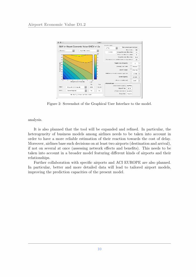
The tool developed in this project could be used for various applications. First,with more detailed airline and passenger data, it could be used as a decision-makingsupport tool for new investments at an airport. For example, the tool could easilyshow if new infrastructures are needed at congested airports, or if incentives to airlinesshould be developed for higher load factors. Moreover, it is easy to use and featuresa Graphical User Interface (GUI), as shown on Figure 2, which allows to exploreinteractively the model.
The tool could also be used by regulators to drive the adoption of new regulationsfor different groups of airports, based on the results of the model and the cluster
9
Airport Economic Value D1.2
Figure 2: Screenshot of the Graphical User Interface to the model.
analysis.
It is also planned that the tool will be expanded and refined. In particular, theheterogeneity of business models among airlines needs to be taken into account inorder to have a more reliable estimation of their reaction towards the cost of delay.Moreover, airlines base such decisions on at least two airports (destination and arrival),if not on several at once (assessing network effects and benefits). This needs to betaken into account in a broader model featuring different kinds of airports and theirrelationships.
Further collaboration with specific airports and ACI EUROPE are also planned.In particular, better and more detailed data will lead to tailored airport models,improving the prediction capacities of the present model.
10

1 Introduction and objectives
The primary objective of the Airport Economic Value project is to assess the valueof additional passengers or additional capacity at an airport. It aims to qualify andquantify the main relationships and trade-offs between capacity, quality of service andprofitability. The purpose of the project is to produce a model capable of capturingthe consequences of the decisions taken by different types of airports, for exampleregarding possible expansion.
In order to do this, the project builds a functional model based on supply and de-mand curves and utility theory embedding causal relationships. Although the AirportEconomic Value model started from a theoretical perspective, the implementation fol-lows a data-driven approach. All modelling decisions are ultimately supported bydata and data analysis only; this encompasses multiple techniques from knowledgediscovery, clustering and factor analysis, among others.
Decisions at the airport are typically based on capacity considerations (both forairlines and passengers), management processes, profitability of added passengers orairlines, and future demand. These decisions result in multiple consequences for air-lines and for passengers, which adapt their behaviour to the new environment providedby the airport. Moreover, the airport usually has to deal with considerable uncertaintyregarding the demand, due to the long-term time frame of the decisions. Airport ex-pectations are thus highly important for the model as they shape the future in whichthe consequences of their actions will be manifested. The final model of the Air-port Economic Value project is able to answer very specific questions related to thesemechanisms, such as the economic viability of the construction of a new runway ata given airport based on several parameters, such as the size of the airport and therequirements of the airport and airlines.
This deliverable presents the final model, the data analysis performed to supportits creation, and the review of the literature and data availability. The aim is topresent work which leads to the implementation of the model, results obtained duringthe design process, the model itself with all its assumptions, and some key resultsobtained from the model. The main text is intentionally concise. Further materialcan be found in the annexes, such as full tables and equations.
The report is organised as follows. Section 2 provides the literature and data
11

Airport Economic Value D1.2
review. Section 3 then details the building process of the model, including the mainresults of the final data analysis. This is followed by Section 4 which presents a shortoverview of the technical implementation of the model, followed by some key resultsobtained with the model. We finally summarise the lessons learnt from the model, andits possible applications, in Section 5. The annexes contain the full technical detailsrelated to data analysis and the model.
12

2 Literature and data availability reviews
2.1 Literature review
Summary
This section reviews the academic and industry literature re-lated to the Airport Economic Value concept by discussing theimplications of airport delays and the options for capacity ex-pansion. The main mechanisms of relevance are ‘soft manage-ment’ processes (such as price schemes, slot allocation strate-gies, etc.) and ‘hard management’ processes (such as infras-tructure improvement). The main variables to consider include:capacity utilisation; traffic mix; aircraft occupation; ‘Net BasicUtility’ (revenues taking the cost of delay into account); thevalue of time of passengers; the share of domestic flights; and,all metrics related to the infrastructures of airports (e.g. thenumber of runways).
2.1.1 The implications of airport congestion and delays
Excess capacity will create minimal delays but will be unprofitable for airports, whichwill be incentivised to utilise their facilities as much as they can, since a significantproportion of their operating costs are fixed, giving a relatively low cost elasticity (0.27(US) [1] and 0.3-0.5 (UK) [2]). Excess demand will produce delay costs for airlinesand passengers [3]. Some airports will pay service-level rebates to airlines when delaysand congestion occurs (4-7% of airport charges at Heathrow and Paris [4], [5]).
The delays will mean that passengers spend longer at the airport and, assumingthat this translates into additional dwell time to use for commercial purchases, thiscan be viewed as a positive externality of congestion [6] This is supported by evidencethat shows that there is a favourable influence of dwell time on passenger spending
13
Airport Economic Value D1.2
[7], [8], [9] with time pressures having a detrimental impact [10]. However, a negativerelationship between unit commercial revenues and passengers has also been found,arguably due to congestion discouraging sales [11] [12] [13]. No direct significantrelationship between commercial revenues and delayed flights has been found [11]although it has been argued that congestion in the terminal should be differentiatedfrom congestion on the runways, since passengers cannot control their time to take-offor shop whilst the aircraft is queuing, whilst they can choose when to arrive at theairport [14].
Airport passenger satisfaction, which is likely to drop with congestion and delays,may also influence commercial spend. At a global level a 1% increase in passengersatisfaction scores is associated with a 1.5% growth in commercial revenues [15] Soeven though greater satisfaction may not directly influence passenger airport choice(this being driven more by locational factors and airline fare/service preferences [16])it may help airport profitability by enhancing commercial revenues. The resultingrelationship between satisfaction and profitability has not always been confirmed [17]as research here is very scarce because of the lack of appropriate and publicly availablesatisfaction data.
2.1.2 Soft management options
In trying to match more closely demand and capacity, the literature discusses twomain options for airports. First, there are so-called ‘soft’ management approaches,that tend to be quick to implement, potentially low cost, but limited in scope asthey do not involve any major changes to the physical infrastructure. ‘Hard’ options,by contrast, are slow to implement and expensive. These can yield large increasesin capacity, because they are lumpy and are made infrequently in relatively large,indivisible units. These two approaches are simultaneously considered by airports,and lead to a two stage optimisation, as shown in [18], with different time frames.
The soft options can relate to both strategic planning and tactical adjustments[19]. In the broadest sense, these can include substituting short-distance air travel withhigh-speed trains, diverting traffic to other airports or using multi-airport systems [20].Related to the airport itself, options may be infrastructure improvement planning [21],[22], changing the ATC rules, and reorganising traffic to make better off-peak use offacilities, or by using aircraft with higher seat capacity, even though this may lead toadditional congestion in the terminals [23], [24].
On the demand side, a major consideration is whether congestion or peak pricingcan be used to manage the traffic. This has been discussed in depth in theory [25]particularly related to the ability of dominant carriers with market power (rather thanbeing atomistic in perfect competition) to internalise the congestion costs. Potentially,peak pricing would push up airline and passenger costs, and bring extra revenuesto the airport, (assuming that it is not introduced in a revenue-neutral manner).
14

Airport Economic Value D1.2
However, in practice, peak pricing has proved difficult to implement and is unpopularwith airlines, particularly since it is viewed as unfairly discriminatory and consideredineffectual in changing behaviour because of complex scheduling operations and slotallocation constraints [26].
Relating congestion pricing to passenger value of time, theoretical research hasdemonstrated that business passengers, exhibiting a greater value, would benefit fromhigher charges to protect them from excessive congestion caused by leisure passengerswith a lower relative value of time [27] [14] and the optimal airport charge would behigher than if passengers were treated as a single type [6]. However in practice airportsdo not discriminate between business and leisure passengers in their pricing, and evenusing airline models types as a proxy (e.g. full service carrier - FSCs, low cost carriers- LCCs) does not hold really true in today’s environment as the distinction betweenthe markets for these two types of airlines is becoming increasingly blurred.
In the short-term, any changes in prices to reflect congestion may not be possibleif the airport is subject to economic regulation, especially incentive regulation, whichtypically places limits on the price increases which are allowed [28]. An alternativedemand management technique, frequently researched [29] [30] and independent ofthe economic regulation mechanism, is a reformed slot allocation process, probablyusing slot auctions or trading systems, which would have major financial consequencesfor airlines and passengers, but less certain impacts on airport revenues.
2.1.3 Hard infrastructure approaches
In discussing the provision of hard infrastructure, it has been argued that the uncer-tainty of future demand [18] and the unpredictability of capacity degradation shouldbe considered [31]. Increasing local capacity can have major unforeseen wider im-pacts, for example, because of the network effects of delays [32]. Trade-offs betweenproviding different types of capacity at departure, and capacity at arrival, have beenidentified [33] and the relationship between runway and terminal capacity examined[14], [34]. It has been contended that the runway capacity should be prioritised sincethis is what causes bottlenecks for most airports [23], [24]. There is also the trade-offbetween focusing on operational and commercial capacity and the extent of comple-mentarity between these two different areas. This is affected by the choice of tillor cost allocation method used when setting prices, with the single till including allairport activities compared to the dual till, when just the aeronautical aspects of theoperation are taken into account [35], [6].
Airports will have different incentives to invest, particularly if they are subject toeconomic regulation. So-called ‘cost-based’ or ‘rate-of-return’ regulation can set in-centives for excessive and too costly investment; price-cap regulation, whilst providingincentives for cost efficiency, can be associated with under-investment. The situationwith light-handed regulation is not so clear [36].
15

Airport Economic Value D1.2
If the airport does invest, growing in size and evolving into a new type of airportwith different operations and/or traffic mix, there will be cost and revenue implica-tions. Larger airports are generally able to provide a greater range of commercialfacilities and services, increasing the commercial spend (less than US $5 per squaremetre for airports of less than 5 million passengers growing to excess of US $30 for air-ports with more than 25 million passengers [37]. Leisure passengers have been shownto spend more than business passengers [11], [9] with some evidence indicating thatLCC passengers spend less [9], [38].
Traffic mix changes will also bring associated costs, related to the service expec-tations of the airlines, such as ensuring a fast transfer time for hub airports, or swiftturnarounds for LCCs. As regards airport size, evidence is mixed but generally itshows that airports experience economies of scale, albeit with different findings re-lated to if, and when, these are exhausted and if diseconomies then occur [39], [40],[41]. As a consequence of these apparent cost and revenue disadvantages for smallerairports, the European Commission (EC)’s view is that airports under 1 million pas-sengers find it hard to cover all of their operating costs, let alone their capital costs.At a size of 3-5 million they should be able to cover all their costs to large extent,whereas beyond 5 million they should be profitable [42].
The costs of any additional capacity can be allocated to airport charges in differentways. There may be a degree of pre-financing, unpopular with airlines, when certaincosts are covered in advance of the capacity becoming operational [43]. Research alsoconfirms the strong influence of market-oriented factors (price sensitivity, competition)on pricing [44], [45]), [46], [47]. The airline’s responses to charge increases will dependon their relative importance to overall costs, with LCCs arguably being the mostsensitive [48]. If charges are passed directly to the passengers, their own sensitivity willreflect the typically quite small influence of charges on airline fares, and subsequentlytheir charges elasticity will be relatively small (estimated at Stansted to be less than-0.15, rising to -0.2 to -0.6 after considering some degree to airport substitution [49],suggesting a fairly marginal impact). However, the evidence is unclear as to the extentto which airlines pass on changes in charges, or whether they choose to absorb at leastsome of these, with a supply-side response to adjust capacity by making changes toroutes and schedules [50]. Irrespective of whether charges are passed on or not, airlinesmay see their profit margins reduced, because any supply response will involve lumpyreductions in airline capacity, having considerable impacts on the passengers [51]. Thisis an example of the wider impacts of capacity provision, which, as with delay impacts,can intuitively be understood but are difficult to support with empirical research.
In summary, this literature review has identified many of the key potential trade-offs relevant to this research. It has discussed the implications of delays at airports andthe various approaches different airports can adopt to increase their capacity. It hasconsidered key airport management issues such as non-aeronautical revenue generationand service quality. This has helped to provide the research context, and to inform
16
Airport Economic Value D1.2
the model where comparisons are made of the marginal costs of extra airport capacitywith the increase in demand due to decreased delays. The review has also coveredthe complex area of airport charging/economic regulation and the wider consequencesfor airline network planning, identifying the difficulties involved with including suchfactors in any trade-off analysis. The overall discussion has enabled an assessment tobe made of the main variables commonly used in the literature, for example relatedto aircraft movements, passengers, airport characteristics and capacities, which hasinformed our own choice of parameters. This now leads on to the consideration ofdata availability.
2.2 Data availability
Summary
Eleven sources of data have been considered and acquired.Data management included data cleaning and small extrapola-tions, as well as cross-checks for plausibility. Data acquisitionand consolidation comprised a large effort within the project.
One of the most intensive efforts of the project has been dedicated to data acquisition,cleaning and consolidation. In order to have a model which could be calibrated asmuch as possible, different kinds of data have been collected. Table 2.1 shows asummary of the data collected, with a brief description of their use.
The reference year for the analyses is 2014, this being the most recent year forwhich the data required were most generally available. A major component was air-port financial and operational data sourced (through subscription) from FlightGlobal(London, UK). ATRS (Air Transport Research Society; USA and Canada) bench-marking study data were purchased, in addition, particularly for the provision ofcomplementary data on airports’ costs and revenues. At the time of analyses, onlyATRS data for 2013 were available, and these selected data were used as a proxyfor 2014. Financial and operational data were compared with in-house, proprietarydatabases, with adjustments made as necessary. Data on airport ownership, and ad-ditional data on passenger numbers, were provided by Airports Council International(ACI) EUROPE (Brussels). European traffic data were sourced from EUROCON-TROL’s Demand Data Repository (DDR) with delay data primarily from the CentralOffice for Delays Analysis (EUROCONTROL, Brussels). Note that, importantly, localturnaround delay is used throughout this work, as this reflects airport in situ effects,whereas air traffic flow management departure delay is generated due to en-route de-lay, or delay at the destination airport - i.e. it is attributable to remote effects. We
17

Airport Economic Value D1.2
Source Typical Content Use
FlightGlobalNumber of flights, number
of passengers, share ofEuropean flights
Cluster analysis,calibration
EUROCONTROL CODADelay per airport & per
typeComparison with DDR
delays
EUROCONTROL DDRFull trajectories of aircraft
for one month of data
Delay distribution,capacity fitting, share of
different types ofcompanies
ACINumber of passengers
(domestic, international,etc.)
Calibration purposes
ACI Ownership airport Not used in final analysesPrivate communication,
EUROCONTROL (2016)Coordination of airport Not used in final analyses
Skytrax, etc Passenger satisfaction Cluster analysis
ATRS Financial dataCluster analysis,
calibration
ATRS Airport chargesComparison with
aeronautical revenues peraircraft
Private communication,EUROCONTROL (2016)
Maximum Take-Off Weight Cost of delay calibration
University of Westminster[3]
Cost of delay Cost of delay calibration
Table 2.1: Data sources, content, and use.
18

Airport Economic Value D1.2
did not have access to clean, local (airport generated) air navigation service (ANS)delay data. Other in-house sources of data were used in addition to those listed, alsodrawing on the literature review.
Considering the wider context of operations in 2014, there were 1.7% more flightsper day in the EUROCONTROL statistical reference area, compared with 2013. Thenetwork delay situation remained stable compared to 2013, notwithstanding industrialaction, a shifting jet stream and poor weather affecting various airports throughout theyear, particularly during the winter months [52]. The average delay per delayed flightdemonstrated a slight fall relative to 2013, and operational cancellations remainedstable ibid. We return to the issue of industrial action shortly.
In the absence of access to a single, comprehensive source of passenger quality ofservice data, airports were assigned an overall passenger satisfaction ranking for 2014,initially based on Skytrax “The World’s Top 100 Airports in 2014” ranking data1, andthen adjusted according to independent reviews by two experts, in addition to somelimited inputs from ACI (Montreal, Canada) drawing on its Airport Service Quality[15] programme data. On this basis, the airports were allocated to a ‘top’, ‘middle’or ‘lower’ ranking. Notwithstanding fairly extensive industrial action in 20142, clearlyimpacting a number of passengers at specific airports, it is difficult to assess the col-lateral (confounding) impact of such events on corresponding passenger satisfactionscores for such airports. The final rankings derived cannot be shown due to confiden-tiality restrictions. This new parameter derived by the team is one of many importantinputs informing the cluster analysis of 3.1.2.3.
To our knowledge, this is the first time that such a very wide range of data hasbeen synthesised in one database and used to characterise airport performance.
1http://www.worldairportawards.com/Awards/world_airport_rating_2014.html2Air traffic control – Belgium: June, December; France: January, March, May, June; Greece:
November; Italy: December. Airlines – Air France: September; Germanwings: April, August,October; Lufthansa: April, September, October, December; TAP Air Portugal: December.
19

3 Model preparation and calibration
The modelling process is presented in this section, as well as the resulting model andthe calibration process.
3.1 Preparing for the modelling process
3.1.1 Using the literature review
The literature review has been used to inform the selection of the main mechanismsand variables for the final model. These are detailed below:
• Airlines are affected by delays through compensation payments and duty of care,as required by Regulation 261 [53], and through the loss of market share arisingfrom reduced punctuality.
• Passenger spending is not directly dependent on the delay at the airport, buton overall passenger satisfaction.
• Airports create delays primarily by operating over or near their capacity thresh-olds.
• Many airport charges are subject to economic regulation and thus charges cannotgenerally be considered as a variable that the airport is freely able to adjust.
• Airport capacity is not a simple value, but rather a concept embedding sev-eral complex and interrelated mechanisms (terminal, runway, gates etc.) anduncertainty.
• Airports are quite diverse in terms of size, business models, types of airlines andpassenger profiles.
• Passenger demand drivers are exogenous to the airport.
20

Airport Economic Value D1.2
These considerations lead to several conclusions. First, it is important to havea model which can be differentiated based on the type of airport considered (hubairport, regional airport, etc.). Second, the impact of delay on the airport resultsfrom airlines being less willing to operate a route because of the corresponding coststhey incur (and possibly as a shortfall in traffic too). Third, uncertainty means thateven levels of traffic under the theoretical airport capacity can imply some delay, andthat the mean average delay is not a sufficient measure for consideration. Fourth,the modelling of the decision-making process of the airport cannot take into accountchanges in airport charges, but merely comparisons of the marginal operational costof some extra capacity with the increase in demand due to decreased delays. Finally,the passenger perspective should not be directly modelled, because passenger choiceof airport is largely independent of factors which can be influenced by the airport.
3.1.2 Using the data analysis
Summary
The data analysis supporting the modelling process is pre-sented. A variable correlation matrix is studied, giving someinsights into the relationships between ‘extensive’ and ‘inten-sive’ variables, infrastructure and traffic data, financial andtraffic data, etc. In order to reduce the complexity of the analy-sis, a principal components analysis shows that the main driverfor variance is the size of the airport, followed by the airportbusiness model and the balance between aeronautical and non-aeronautical revenues. A clustering analysis divides the mainairports into three communities, which are roughly consistentwith expert judgement.
3.1.2.1 Correlations
One of the challenges of constructing a comprehensive model for an airport is inbuilding causal relationships between a small number of core variables. The choiceof these core variables is determined by considering the dependencies of the differentvariables on each other in the data. The first step is thus to compute the correlationcoefficients between each variables as these give the magnitude of the linear statisticalcorrelations. The table of correlations can be found in Annex A.1, as well as thedifferent variables considered and their meaning.
21

Airport Economic Value D1.2
Airport operating revenues are strongly correlated with several metrics, includingthe number of passengers and the number of flights, which is expected, but also withaircraft occupation (number of passengers per flight) and the number of passengers perroute, with correlation coefficients as high as 0.97. This is especially striking becausethe latter metrics are not trivially linked to the number of passengers or flights, so itis not a simple scaling effect. In fact, it shows how ‘extensive’ variables, i.e. scalingwith the number of passengers or flights, can interact with ‘intensive’ variables. Theseeffects are very important to capture, because intensive variables usually reflect thefundamental organisation of the system, related to the interaction between differentagents (e.g. some kind of management rule). Regarding the precise meaning of thiscorrelation, it is not clear at this stage why the operating revenues should be so closelyrelated to these metrics, except if they are linked to some kind of capacity, as discussedbelow.
More interestingly, some of the intensive variables, like aircraft occupancy, are cor-related with the size of the airport (0.61). This is also expected since small airportsusually have more versatile functionality, which requires smaller aircraft for flexibility.Other features are worth exploring. For instance, the proportion of intra-Europeanflights seems to be strongly (negatively) correlated with different variables, includingthe total number of flights and number of gates (-0.77 and -0.65, respectively). Thiswas expected since intercontinental airports are also the largest ones. More impor-tantly, total delays seem to be positively correlated with the number of runways, thenumber of gates and the number of terminals (0.41, 0.58, and 0.45, respectively), i.e.with the size of the infrastructure. This is because longer delays are expected at thebigger airports, which have the largest infrastructure. On the other hand, the delayper flight is less correlated with the infrastructure (0.38, 0.34, and 0.2). This is a goodsign, because it could mean that the airports increase their infrastructure to counter-balance delays. It is also observed that runway and terminal usage have non-trivialbehaviour with respect to the number of runways and terminals, since they are weaklyor negatively correlated with them (-0.25 and 0.02), which could loosely mean thataverage airports are ‘over-building’, i.e. the number of runways and the number ofterminals increase more quickly than the number of passengers. Note that, strangely,the terminal usage increases (weakly) with the number of runways (0.25), whereasthe runway usage is quite independent of the terminal usage. This is the productof a subtle co-evolution of different capacities, namely the terminal capacity and therunway capacity.
Indeed, this is typically where simple correlation scores begin to show their limit.It is not clear at this point what are the drivers of the different metrics and whethera few causes only can explain most of the correlations. In order to explore this, weturn now to principal components analysis (PCA).
22

Airport Economic Value D1.2
3.1.2.2 Principal components analysis
Since there are different types of airports, this is likely to have major consequencesthat should be reflected in the model. Rather than relying on purely expert-drivenclusters, the clusters are defined in a data-driven way. In order to do this, a fewvariables of importance in the data were selected, which are presented in Table 3.1.We tried to select different types of variables with the most reliable data. Clearly,some of the variables are correlated, as shown in the correlation table in Annex A.1.In order to have a better picture, the decision was made to use PCA, reducing thenumber of independent variables to four, while keeping 80% of the initial variance.
Abbreviation Short descriptionAO tot Number of airlines
CUI Capacity utilisation index
NBUNet basic utility
(net operational incomeminus costs of delay)
cap Runway hourly capacitycht Share of low-cost carriers and chartersfsc Share of full-service carriers
delay per flight Delay per flightdelay tot Cumulative turnaround delayexp tot Total yearly expenses
flight EU Share of European flightsflight per rnwy Flights per runwayflight per term Flights per terminal
flight tot Total number of flightsgate tot Number of gatesterm tot Number of terminals
pax per flight Passengers per flightpax tot Number of passengersrev areo Aeronautical revenues
rev non area Non-aeronautical revenuesrnwy tot Number of runwaysroute tot Number of routes
sat Passenger satisfaction
Table 3.1: Variables used to characterise the airports.
Indeed, the objective of the PCA is to explain as much variance as possible in thedata, and this is generally a key indication of the quality of the solution. However,
23

Airport Economic Value D1.2
it is not acceptable to obtain a purely ‘mathematical’ solution in the analysis, i.e.whereby the analyst is not able to assign real meaning to the factors, which may be achallenge when there are too many of them. There is thus usually a trade-off betweenthe number of components and the amount of variance explained.
It is also often desirable to ‘rotate’ the factors, to increase loadings on some of theoriginal variables, and decrease them on others, in order to ease the interpretation ofthe solution and improve its simplicity. Thus to allow for a better interpretation ofthe results, we used varimax rotation. This is an orthogonal rotation method thatminimises the number of variables with high loadings on each factor [54].
After this procedure, the four new components – linear combinations of the ini-tial variables – have the weights displayed in Figure 3.1. The new variables explain
Figure 3.1: Weights of the initial variables for each component.
approximately 46%, 9%, 14% and 9% of the variance, respectively. The remainingvariance (22%) can be explained by additional components, but the more we have,the less they are individually significant. For instance, the next component only ex-plains 5% of the variance. Presenting four components, explaining some 80% of thevariance of ∼30 initial components, is sufficient to draw reasonable conclusions, evenif their interpretation is not completely straightforward.
24
Airport Economic Value D1.2
The first component (labelled 0) is homogeneously composed of all initial vari-ables, in particular the ‘extensive’ variables such as the total number of flights or thenumber of delays. Hence, this first variable can be seen as the ‘size’ of the airport,which appears to be the main driver of most of the initial variables, because this firstcomponent accounts for almost half of the variance.
The second one (labelled 1) is clearly linked to the type of airlines which areoperating at the airport. Specifically, it seems that 9% of the variance is closelyrelated to the fact that airports serve more traditional/full-service carriers or morelow-cost carriers. It is also evident that the infrastructure is closely linked to this,since the number of runways and terminals play a large role in this component too.Interestingly, the component is related to the number of passengers per aircraft, whichis low when the component is low, i.e. when the airport is more ‘low-cost-oriented’– in spite of pressures on these airlines to be punctual and have minimal turnaroundtimes. This is not unexpected, since low-cost carriers often operate smaller aircraft,especially as they have very little long-haul traffic. It is also worth noting that thedelay per flight increases when the airport is more ‘low-cost-oriented’.
The third component (labelled 2) is related to the financial state of the airport,with net basic utility and non-aeronautical revenues playing major roles. Interestingly,the total number of runways has a positive impact on this component, whereas thenumber of terminals has a negative effect. Since the capacity being measured islinked to the air traffic movements, it is clear that it has an impact on the componentaccordingly with the number of runways.
Finally, the last component (labelled 3) is linked to the physical infrastructure ofthe airport, which affects its usage (number of flights per runway and per terminal),but also the passenger satisfaction.
3.1.2.3 Clustering
Having defined a smaller number of variables with a clearer understanding of theirmeaning, we now cluster the airports, gathering together the ones which are similarin the same ‘community’. Note that in this part, the number of airports considered isequal to 32, which are the airports for which all the fields of table 3.1 are informed.Together, they represent more than half of the traffic in Europe in terms of passengers(53%).
There are many different ways of clustering data, depending on the definition of‘clustering’. Several methods are routinely used in the literature but the specific choiceof method is always quite subjective.
Indeed, the problem of clusterisation in community detection is mathematicallypoorly defined. The main reason is that the definition of a ‘cluster’ or ‘community’is subjective, and varies among the different fields in which it is used. As a result,one should first define what one thinks would be the ‘right’ definition of a cluster
25

Airport Economic Value D1.2
in the particular context, before trying to find the right method. In this research,we are interested in discovering whether some airports have similar behaviours. Thesimplest and most accurate way of finding this, it is proposed, is through the use of aEuclidean distance of their different characteristics, weighted by the PCA results. Thebest definition of a cluster is then related to the probability of two airports being closer(in terms of this Euclidean distance) to each other, than to the rest of the network.This technique, from network theory (and based on modularity), thus presents itselfas being appropriate.
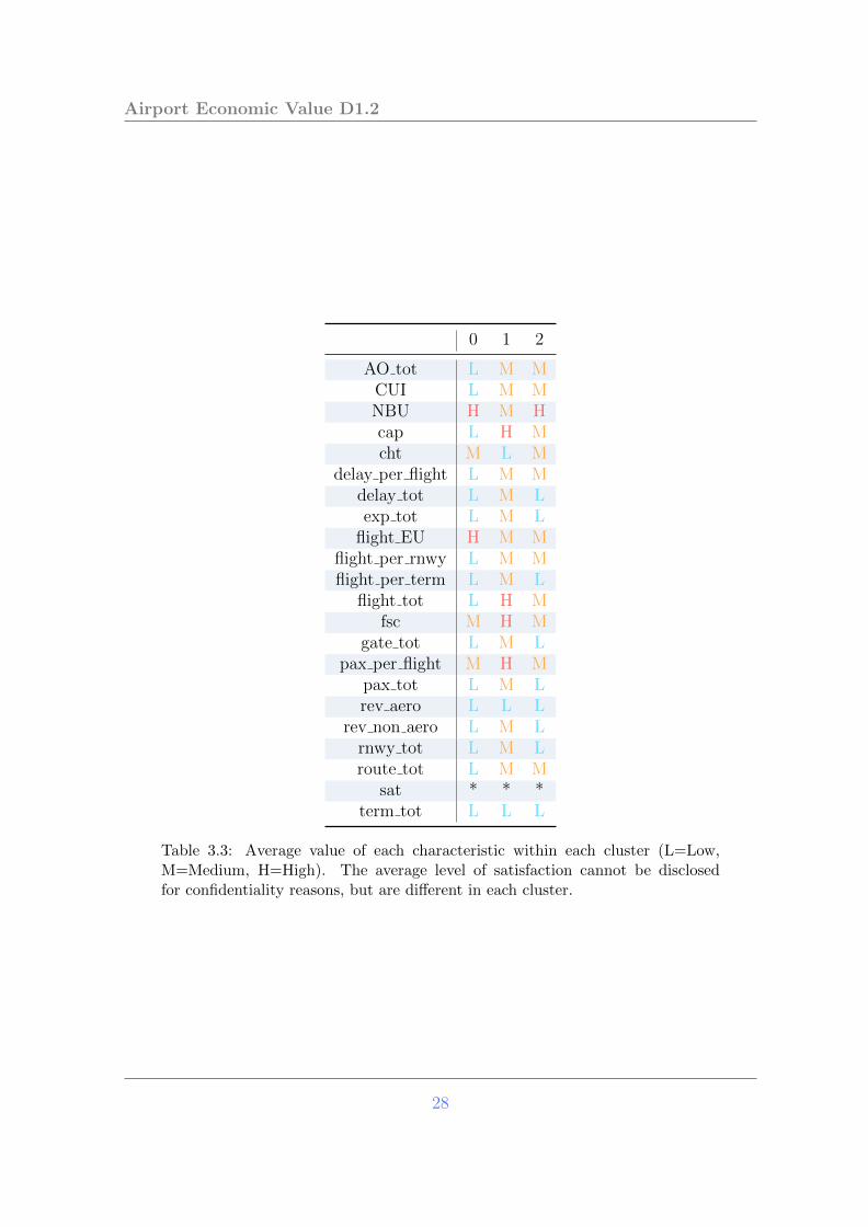
The details of the method can be found in Annex A.2. Here, we emphasise thefact that the previous PCA was directly integrated with the clustering analysis, sincewe used as distance between airports the Euclidean distance of the four componentsof the PCA, each weighted with their ratios of variance explained. In the same annex,we also show how we checked that the partition is robust with respect to uncertaintyin the data. This partition is presented in Table 3.2. Cluster 1 includes mostly majorhubs, whereas clusters 0 and 2 include airports with less traffic. Cluster 2 contains anumber of secondary hub airports.
In order to inspect the clusters more closely, we also show in Table 3.3 the aver-age value of each of the airports’ characteristics, according to three categories: low,medium and high. Upon inspection of the table, the difference between clusters 0and 2 appear more clearly. Indeed, the first one includes airports which have pro-portionally lower delays per flight, fewer routes, lower passenger satisfaction, fewerflights, and less congestion (lower CUI value) with respect to cluster 2. The tablealso confirms the status of ‘major hubs’ of the airports of cluster 1, with high num-bers of passengers, numbers of flights, revenues and expenses. It confirms a tendencyof such hubs to attract non-low-cost carriers, to experience higher delays per flight,and to have a more international profile. Interestingly, the passenger satisfaction isalso different in this cluster, although the average level cannot be disclosed (for rea-sons of confidentiality). The net basic utility is not so high, however, probably drivenby higher delays per flight, whereas the load factor is high for major hubs, as expected.
The cluster analysis thus gives us a suitable basis on which we can build differenti-ated models. In the following analysis, we use it to simplify some parts of the model.Taking into account the full diversity of the airports is not necessary.
26

Airport Economic Value D1.2
Cluster Id ICAO Code Airport Name
2 EBBR BrusselsEDDL DusseldorfEGCC ManchesterEIDW DublinEKCH Copenhagen KastrupENGM Oslo GardermoenESSA Stockholm Arlanda
LOWW ViennaLPPT Lisbon
1 EDDF FrankfurtEDDM MunichEGKK London GatwickEGLL London HeathrowEHAM Amsterdam SchipholLEBL Barcelona-El PratLEMD Madrid BarajasLFPG Paris Charles de GaulleLIRF Rome FiumicinoLSZH ZurichLTBA Istanbul Ataturk
0 EDDH HamburgEDDK Cologne BonnEFHK HelsinkiEGBB BirminghamEGSS London StanstedELLX LuxembourgEPWA Warsaw ChopinLFMN Nice Cote d’AzurLGAV AthensLHBP BudapestLKPR PragueLPPR Porto
Table 3.2: Composition of the partition from the clustering analysis. Theseairports combined represent 53% of the traffic in number of passengers.
27
Airport Economic Value D1.2
0 1 2
AO tot L M MCUI L M MNBU H M Hcap L H Mcht M L M
delay per flight L M Mdelay tot L M Lexp tot L M L
flight EU H M Mflight per rnwy L M Mflight per term L M L
flight tot L H Mfsc M H M
gate tot L M Lpax per flight M H M
pax tot L M Lrev aero L L L
rev non aero L M Lrnwy tot L M Lroute tot L M M
sat * * *term tot L L L
Table 3.3: Average value of each characteristic within each cluster (L=Low,M=Medium, H=High). The average level of satisfaction cannot be disclosedfor confidentiality reasons, but are different in each cluster.
28

Airport Economic Value D1.2
3.2 High-level principles of the modelling process
Summary
Important mechanisms and variables are considered and jus-tified in this section. Airport congestion creates delay for theairline, and thus economic loss. An airline may decide not tooperate from the airport if the cost is too high. The airportmay increase capacity, which decreases the delay, but has anoperational cost. The revenues of the airport are dependant onthe number of flights (aeronautical revenues) and the numberof passengers (non-aeronautical revenues).
In this section, the model used for the final version is presented. The correspond-ing equations, with some more details, can be found in Annex B.2. The model is asimple functional model based on representative agents, with the following fundamen-tal principles.
First, we use a functional relationship linking the delay at an airport with thecapacity and traffic. The progression is exponential (based on regression, see the cal-ibration Section 3.3). The delay is then converted into a cost for the airline, based onthe average maximum take-off weight (MTOW) at the airport. The cost is quadraticwith the delay [3], which means that longer delays have proportionally higher coststhan shorter ones.
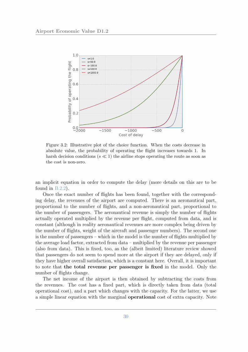
This cost then fixes the probability that the airline actually operates the flight,through a probability function based on a hyperbolic tangent function. This choice ismotivated by the fact that this probability is linked to some form of utility functionfor the airline, taking into account other (strategic) parameters (as described above).It allows us to have a smooth function which varies continuously between 0 and 1, andto have a ‘risk aversion’ of the agent which can directly be linked to the parameter s –henceforth referred to as the ‘smoothness’ of the decision. Indeed, when s is sufficientlysmall, the airline takes ‘harsher’ decisions, switching from operating to non-operatingthe route once costs are driven high enough. This behaviour is illustrated in Figure3.2. Note that, in fact, we should strictly be referring to the net revenue contributionto the network, since airlines will tolerate loss-making legs that have a net benefit tothe system. This parameter is the only behavioural parameter of the model and theonly free parameter.
Note that the probability depends on the delay, which depends on the traffic, whichin turn depends on the probability itself. As a consequence, there is a need to solve
29
Airport Economic Value D1.2
Figure 3.2: Illustrative plot of the choice function. When the costs decrease inabsolute value, the probability of operating the flight increases towards 1. Inharsh decision conditions (s� 1) the airline stops operating the route as soon asthe cost is non-zero.
an implicit equation in order to compute the delay (more details on this are to befound in B.2.2).
Once the exact number of flights has been found, together with the correspond-ing delay, the revenues of the airport are computed. There is an aeronautical part,proportional to the number of flights, and a non-aeronautical part, proportional tothe number of passengers. The aeronautical revenue is simply the number of flightsactually operated multiplied by the revenue per flight, computed from data, and isconstant (although in reality aeronautical revenues are more complex being driven bythe number of flights, weight of the aircraft and passenger numbers). The second oneis the number of passengers – which in the model is the number of flights multiplied bythe average load factor, extracted from data – multiplied by the revenue per passenger(also from data). This is fixed, too, as the (albeit limited) literature review showedthat passengers do not seem to spend more at the airport if they are delayed, only ifthey have higher overall satisfaction, which is a constant here. Overall, it is importantto note that the total revenue per passenger is fixed in the model. Only thenumber of flights change.
The net income of the airport is then obtained by subtracting the costs fromthe revenues. The cost has a fixed part, which is directly taken from data (totaloperational cost), and a part which changes with the capacity. For the latter, we usea simple linear equation with the marginal operational cost of extra capacity. Note
30

Airport Economic Value D1.2
that this is not the cost of the infrastructure itself (e.g. runways, terminals), sincewe are interested in the recurring costs only, and not fixed lump sums associated withmajor investments.
Finally, in order to have an idea of the impact of delay on passengers, we com-pute a utility function based on value of time, which is a function of the share ofbusiness passengers at the airport. As an approximation for this, we use the shareof traditional/full-cost carriers at the airport, as opposed to low-cost, although it isacknowledged that a growing share of business travellers now use low-cost carriers.
The model is not only based on average values, since one of the key features ofthe cost of delay is its non-linearity with the delay. As a consequence, we use certaindistributions for the traffic and integrate the other values of the model with the traffic.More details about the types of distributions that we use are given in the followingsection on calibration.
3.3 Calibration
Summary
The model’s calibration is presented. Data are used in threeways: (i) directly estimating input parameters for the model;(ii) extracting functional relationships from the literature ordata regression; (iii) tuning input parameters by matching anoutput metric of the model to a target value from the data.The fully calibrated model has only two free parameters: themarginal operational cost of additional capacity and an internalbehavioural parameter. The results are not strongly dependanton the latter, and it could in principle be post-calibrated usingthe average delay returned by the model. The first parametershould be considered as a variable, or be precisely estimated forindividual airports.
Here we describe how we calibrate the model. The calibration itself is performed invarious steps. Indeed, some parameters can be calibrated directly from the data, butsome need to be swept, matching an output of the model to the corresponding valueextracted from data. Moreover, we need different functional relationships comingdirectly from data.
31

Airport Economic Value D1.2
3.3.1 Functional relationships
The first functional relationship we use is the one between the traffic and the delay.In order to compute it for each airport, we used DDR data, with the use of thedifference between M3 (actual, radar-tracked flight) and M1 (last-filed flight plan)departure times as an approximation for the real delay. In appendix B.1.1, we studythe potential difference between these delays and the real ones, that are only availableat an aggregated level from CODA data (and not throughout the day). We use onemonth of data, and we compute the number of departures during each hour of eachday, as well as the corresponding mean delay. We then average them over the wholemonth of data and for each airport, and perform an exponential fit. There are onlytwo parameters to the fit, one of them being a measure of the capacity. Finally, theairports were gathered according to the three clusters found in Section 3.1.2.3, whichmeans that we use only three relationships in total.
The passenger costs cover compensation and duty of care, as required by Regu-lation 261 [53], and also reduced market share costs arising from poorer punctuality(they do not include (internalised) passenger value of time costs). The delay costsare sourced from [3]. Based on this source, we carried out a regression fit for primarydelay (to avoid double-counting across the network by including reactionary impacts)costs using the weights of the aircraft and the delay durations. The final function is:
cd = −7.0 δt− 0.18 δt2 + (6.0 δt+ 0.092 δt2)√MTOW, (3.1)
For the model, we set√MTOW to its average across all aircraft departing from the
airport.In this equation, the delay should not be an average one, but the actual delay of
each flight. This is a potential issue for the model, given that we are using average de-lays (per hour). Indeed, it is clear, for instance, that a null average delay still producesa cost, since some flights are still delayed, and thus bear a cost, whereas airlines withflights ahead of schedule are assumed not to benefit financially (they may even suffercosts). Moreover, the cost is super-linear with the delay, which means that long delayscost proportionally much more than shorter ones. As a consequences, we used DDRdata to compute the intra-hour distribution of delays. These distributions are fittedwith log-normal distributions (see Annex B.1.3), which is a suitable approximation,even though very long delays are sometimes underestimated. The previous equationis then corrected, using the expected values of the cost, based on the probabilitydensity of delays. This procedure is undertaken airport by airport, increasing thetotal real cost. Note that, in particular, the expected cost of delay for a null averagedelay is not null any more.
32

Airport Economic Value D1.2
3.3.2 Direct calibration of parameters
Some parameters can be directly estimated from the data, for each airport:
• The load factor lf is given by the ratio of the number of flights and the number ofpassengers (this is not the real average load factor which would need to considereach flight separately).
• The (average) aeronautical revenues per flight P are given by the total aeronau-tical revenues divided by the number of flights.
• The (average) non-aeronautical revenues per passenger w are given by the totalnon-aeronautical revenues divided by the number of passengers.
• The distribution of traffic {T} through the day is fixed by averaging one monthof data, splitting the day into 24 hour periods.
The value of time for all passengers, not useful per se for the model but impactingon passenger satisfaction, can be found in the literature. To have a more realisticdescription, we decided to use two values of time, which are usually associated withbusiness (vb) and leisure passengers (vl), sourced from [55]. We then consider thatmost passengers on low-cost carriers have a lower value of time – often associated withleisure trips – whereas passengers travelling with traditional/full service airlines havea higher value of time, reflecting more business trips. As a consequence, the averagevalue of time in our model is:
v = vlrlcc + vb(1− rlcc),
where rlcc is the share of low-cost carriers at the airport. This value is also directlytaken from data (i.e. DDR data). Note that this is a very crude approximation, sincemany business-purpose trips are made on low-cost carriers, for example. However,since precise passenger profiles are not currently available to the research team, thisis a reasonable approximation, and better than simply considering as equal businessand leisure passenger volumes across all flights.
Finally, an important parameter is the marginal cost of extra capacity per pas-senger α. This value is quite difficult to extract from data, so we consider it as afree parameter most of the time. However, in order to have an approximate idea ofits value, one can assume that the main objective of an airport is to deliver capacity,and thus all of its costs should be related to this delivery. A regression of the totalcosts is thus carried out (outlay on infrastructure, such as a new runway) for thevarious airports, as a function of capacity. A linear regression is reasonable in thiscase (R2 = 0.53) except for the high cost airports (essentially CDG, LHR, and FRA).The cost is thus around 24 000 euros per unit of capacity per day. This correspondsto 220 euros per passenger, per day, taking CDG as an example.
33

Airport Economic Value D1.2
3.3.3 Post-calibration of parameters
We call post-calibration the operation of running the model with different values of oneor more parameters, and comparing an output of the model to some values extractedfrom the data.
With the final version of the model, we only need to post-calibrate one parameter(β), tuning the demand at the airport. More specifically, it is a multiplicative factor forthe traffic. When calibrating this, we match the effective number of flights operated atthe airport with the real ones in the data, sweeping the value of β. After calibration,β is usually a value greater than 1. Indeed, we need to increase the traffic volumesobtained from data, since the probability that the airline operates the flight is smallerthan 1. In other words, we compensate for the disincentive of airlines (i.e. due to thecost of delay) associated with an increase in demand, in order to match the observednumber of flights.
3.3.3.1 Summary of calibration
In summary, the calibration includes the following steps:
• Maximum take-off weight MTOW is included in the cost-delay relationship.
• Average load factor lf , aeronautical revenues per flight P and non-aeronauticalrevenues per passenger w, value of time v, total initial cost cinit, and distributionof traffic {T} through the day are taken directly from data.
• Fitting parameters cc and Cinit (the latter being the capacity) for delay-trafficload relationship are set.
• Cost of delay relationship is corrected based on intra-hour log-normal fittingdistributions of delays.
• Demand factor β is post-calibrated by matching of the number of flights withthe data.
The ‘total initial cost cinit’ represents the total current costs of the airport, i.e. costsfor providing the current capacity. Finally, we have two parameters remaining, thesmoothness of the airline decision s and the marginal cost of capacity α, which is theoperational cost of running one extra unit of capacity. The latter could be estimated,for instance, with the current cost per passenger, but we prefer to keep it as a variable,since the exact figure is likely to be different from just ‘capacity/passengers’.
The smoothness is thus the last free parameter of the model. It represents thesensitivity of the airline to the cost of delay. The higher it is, the smoother thedecision will be, i.e. the airline will not suddenly cease operating at an airport when
34

Airport Economic Value D1.2
the cost increases. When the decision is harsh (low value of s), the airline ceases tooperate the flight as soon as the cost is non-zero.
It is clearly linked to the elasticity of demand (associated with the airline) and thecost (of the airline operating a flight at the airport), which is very hard to estimatebecause of lack of detailed airline data. It is worth noting, however, that:
• a basic sensitivity analysis (see Annex C) shows that the results of the modeldo not depend strongly on the value of s,
• the parameter is actually not totally free, but is constrained at low values. Thiscomes from the fact that a low elasticity cannot fulfil demand requirements.
As a result, the model is only slightly over-fitted and thus suitable for the task.
In Table 3.4, we present a summary of all the parameters1 and their types, corre-sponding to the ways that they are calibrated.
Name of parameter Short descriptionType of
parameterValue for
calibrated airport
MTOW Max. take-off weight DC 120 euroslf Load factor DC 271 pax/flightP Airport charges DC 2393 eurosCinit (Departure) capacity DC 35.59 flightscc Delay at zero traffic DC -1.83 minutesv Value of time DC 39.91 eurosT Distribution of traffic DC (distribution)w Average revenue per passenger DC 17.78 euroscinit total initial cost DC 3.3m eurosβ Traffic multiplier (demand) PC 3.45 (no units)α Marginal cost of capacity FP –s Smoothness FP –
Table 3.4: List of parameters of the model, with their types related to calibration.DC: Direct calibration, FP: Free parameter, PC: Post-calibrated. The last columnpresents the value obtained for the calibration with the selected airport.
Once the model is calibrated, it is possible to change some of the parameters tosee the impact on other variables, as is demonstrated in the next section.
1This list of parameters is different from the metrics considered in the data analysis section.Indeed, only those parameters were selected that could be included in the model and calibrated.Many of the parameters of the data analysis were included at first in the model, but were thenremoved as progress was made to a fully calibrated model.
35

4 Model implementation and results
4.1 Implementation
Summary
The model is implemented in Python and uses a MATLABgraphical user interface (GUI) for user-friendly interactions.The user can change the values of different parameters, and theoutput representation, for a seamless experience of the model.
4.1.1 Engine implementation
The model is written in Python and is divided into two parts. The first relates to thecalibration, where relevant data are extracted from our sources and several operationsare performed to prepare the model, such as regressions. The output of this part isa Python object embedding all the calibrated parameters. The second part of thecode is the object itself, which is able to produce different outputs based on the freevariables passed in the inputs. The output is then used by the graphical user interface(GUI), described below.
4.1.2 Graphical user interface (GUI)
The model developed is aimed at experts in air transport, that do not necessarilyhave the technical or programming skills to execute or modify a software platform.In order to make the model more accessible, a visualisation layer, or GUI, has beendeveloped on top of the data-driven, ‘back-end’ model (engine). The model is thendelivered as an autonomous piece of software usable without programming skills.
This visualisation helps the user to understand the underlying model behaviourand evolution when varying certain input parameters and airport types, for exampledetermining the combination of parameters that lead to desirable outputs or, in some
36

Airport Economic Value D1.2
cases, optimum values. The visualisation tool also helps to determine the stabilityand sensitivity of the optimal points, the local behaviour in small neighbourhoods,visually.
Figure 4.1: Screenshot of the visualisation layer.
The engine has been developed in MATLAB and can be deployed on Windows, Macand Linux platforms. It is packed as a MATLAB standalone application. Therefore, alicensed copy of MATLAB is required. If not available, MATLAB runtime needs to beinstalled. (Instructions for installing MATLAB standalone applications and runtimelibraries can be found at [56].) The engine is compatible with modules (airport andairline models) written either in MATLAB or Python programming languages andexports output data into common formats: .png for figures, plus .xml and Excel-compatible .csv files for tables. Although the visualisation layer has been developedas intuitively as possible, embedded in the software, there is a user manual to facilitatethe use of the GUI. It can be accessed from the ‘Help’ menu at the top right-handcorner of the application window, as shown in Figure 4.2.
Source codes are stored in a private and secure GitHub repository. GitHub is anonline control version repository with collaborative capabilities. Updates, bug fixesand new versions of the model will be released beyond the current project. Snapshotsas a MATLAB standalone application could be made on demand. The source codewill be hosted and maintained indefinitely.
37

Airport Economic Value D1.2
Figure 4.2: Help menu.
4.2 Calibrated model results
Summary
The model calibrated on a large, European hub airport showsthe presence of an optimum in capacity greater than the currentcapacity, for a wide range of marginal operational costs. At theoptimum, the mean delay has fallen by approximatively 5% andthe passenger utility has increased by the same amount. Whencalibrating different airports, one can compare the maximumoperational cost for which a given increase is profitable to theairport. As expected, bigger airports can, in general, sustaingreater extra operational cost, in particular because they arethe most congested. However, the number of passengers is notthe only factor, and some large airports cannot sustain highoperational costs.
4.2.1 Calibrated airport
We have two free variables. The first is the new capacity C targeted by the airport,and the second is the marginal cost of capacity α. All other variables have beencalibrated, as described previously.
Figure 4.3 shows the net income of the airport when changing these two variables.The global maximum is clearly reached when the marginal cost is null and the capacityis at its maximum value. It is interesting that, for a given value of α, there are twopossibilities: either there is a maximum in capacity, or there is not. Indeed, for asmall value of α, when the capacity increases, the net income also increases, up to acertain point, after which it starts decreasing. This is because increasing the capacity
38

Airport Economic Value D1.2
decreases the delay, and more flights are operated. However, in contrast, the incomeper passenger decreases with capacity, as we explain below.
Figure 4.3: Evolution of the net income of the airport as a function of the capacityand the marginal operational cost.
In order to see this effect more clearly, we present various graphs in Figure 4.4,where we have fixed α = 60k. Starting from the top left, graph (a), we first show therevenues per passenger, which in our model is a constant. Indeed, only the number offlights, and thus the number of passengers, change when the capacity is altered. Notethat in reality, there might be two different opposite effects related to this. On the onehand, the non-aeronautical revenues have been found to be weakly correlated withpassenger satisfaction. As a result, increasing capacity may increase the passengersatisfaction, and hence the non-aeronautical revenues per passenger. On the otherhand, it may be possible that some diseconomies of scale might occur when the airportis handling more passengers and reaches a certain size threshold, as discussed in theliterature review.
Graph (b) shows the cost of capacity, which increases with the number of pas-sengers. This is the case because increasing capacity by one unit does not bring allthe potential passengers, but only a fraction of them. As a result, the income perpassenger decreases with the capacity, as shown in graph (c).
In graph (d), we show that average delay decreases with capacity, which is themain objective. As a consequence, the cost of delay for airlines decreases too (graph
39

Airport Economic Value D1.2
(e)), and the airport serves the demand better (graph (g)), with a higher number offlights (graph (h)).
The relationships between the increase in the number of passengers and the de-crease in the net income per passenger leads to a maximum for total net income(at least for some values of α), see graph (i)). Finally, as average delay decreases,passenger utility monotonically increases (i.e. with better satisfaction), see graph (j).
Figure 4.4: All results are expressed per day. Evolution of (a) revenues perpassenger, (b) cost per passenger, (c) net income per passenger, (d) averagedelay per flight, (e) cost of delay per flight, (g) ratio between operated flightsand demand, (h) number of flights actually operated, (i) total net income of theairport, and (j) passenger utility, as functions of the airport capacity.
4.2.2 Comparing different airports
In order to compare the different airports, we identify the value of α for which thenet income of the airport reaches a maximum, when the capacity is increased by 50%
40

Airport Economic Value D1.2
with respect to its current value. This gives a rough idea of the maximum marginalcost at which it is profitable to increase the capacity. Table 4.1 show the results forvarious airports, as well as some other metrics, for comparison. It is striking to seehow this typical marginal cost varies significantly among airports, from LPPR with541 euros, to EGLL with 83 540 euros. This means, roughly, that an increase of 50%of the capacity at Heathrow is profitable up to a marginal operational cost of 83 540euros per day per unit of capacity. On the other hand, an increase of 50% of thecapacity for Porto airport would be profitable only if the marginal operational costwere below 541 euros per day.
C α Pax (millions) CUI
EDDF 37.6 43087 59.6 0.54EDDH 14.3 10404 14.8 0.49EDDK 40.7 5106 9.45 0.53EDDL 35.5 5106 21.9 0.49EDDM 73.5 19038 39.7 0.52EFHK 29.6 5586 15.9 0.44EGBB 10.5 1424 9.72 0.45EGCC 14.9 3409 22.1 0.47EGKK 20.2 6127 38.1 0.61EGLL 28.7 83540 73.4 0.59EGSS 17.5 7148 19.9 0.49EHAM 50.2 29615 55.0 0.53EIDW 45.5 4085 21.7 0.59EKCH 45.0 8477 25.6 0.49ESSA 30.8 3179 22.5 0.53LEMD 29.9 17687 41.8 0.55LFPG 41.3 53073 63.8 0.54LGAV 13.1 7014 15.2 0.44LIRF 288.9 8323 38.5 0.51LOWW 34.3 8784 22.5 0.46LPPR 4.7 541 6.93 0.37LPPT 16.5 2234 18.1 0.49LSZH 26.1 8630 25.4 0.53LTBA 12.8 3179 56.7 0.67
Table 4.1: Capacity, typical marginal cost for which an increase of 50% of thecapacity is profitable, number of passengers and capacity utilisation index for allcalibrated airports.
It is interesting to see that this threshold seems to be highly correlated with the
41

Airport Economic Value D1.2
size of the airport (see Figure 4.5), in a quite non-linear way (the initial analysis showsthat it is compatible with a power law). This could be related to economies of scaleas discussed in the literature review.
Figure 4.5: Threshold of the marginal cost of capacity for which an increase 50%of the capacity is profitable for different airports.
4.2.3 Effect of parameters on the position of the optimum
In this section we examine the effect of the various parameters on the position of theoptimum. Since all the parameters are calibrated, or considered as variables, someparts of the calibration procedure are relaxed to allow some of the parameters to vary.
The first parameter that we are interested in is the load factor. As highlighted inthe literature review, the average load factor at airports has been increasing in recentyears, except at highly congested airports. The main reason is that this is a relativelycheap way of increasing their effective capacity. As a consequence, many of them tryto find incentives for airlines to increase the size of their aircraft.
In the calibrated model, the load factor lf is derived simply by dividing the totalnumber of passengers by the total number of flights for a given airport. Here, we relaxthis calibration and sweep the parameter, every other parameters being unchanged.This load factor in our model has a very simple effect: it increases the non-aeronauticalrevenues linearly. As a consequence, the optimal capacity is shifted, as shown in Figure4.6. The figure shows the optimal capacity as a function of the load factor.
42

Airport Economic Value D1.2
Figure 4.6: Optimal capacity as a function of the average load factor.
For low load factors, the optimal capacity is at the current capacity or below (bydesign, here the capacity cannot fall below the current value). At a certain point, theload factor is high enough, and the optimal capacity starts to increase linearly withit. This simple effect is due to the fact that higher load factors act as a “free” increasein capacity, and thus the airport has less need to increase actual infrastructure.
The second interesting feature that we study is the effect of predictability whenpunctuality is fixed. In other words, the effect of the variance of the delay when themean delay is fixed. To simulate this effect, we change the ’correction term’ of the costof delay function, reducing progressively the variance of the log-normal distributionwhile keeping a constant mean.
First in Figure 4.7, we show the impact of decreasing predictability on the cal-ibrated model with the current capacity, for different metrics. The right-hand sideof each graph corresponds to the situation in the data, i.e. a normalised standarddeviation of 1. The extreme left-hand side corresponds to a perfectly predictable sit-uation, but not perfectly punctual. This last limit is not very realistic and the modelprobably fails in this region, due to the fact that in reality airlines would integrate asimple off-set of departure times into their objective functions.
Nevertheless, moderate increases of predictability (decreases of standard deviation)are probably well captured by the model. Unsurprisingly, the net income starts byincreasing when the standard deviation falls. This is due to the fact that it is lesscostly for airlines to operate at this airport, and thus they are more willing to do so.However, the net income is not monotonic - we return to this point later.
We first focus on the average delay at the airport. The counter-intuitive results
43

Airport Economic Value D1.2
Figure 4.7: Evolution of different metrics with the increase of the standard devi-ation of delay at the airport (decrease of predictability).
44

Airport Economic Value D1.2
from the model indicate that increasing the predictability actually increases the meandelay at the airport. Apparently, the airport trades the extra predictability againstsome extra average delay, in some kind of mean-variance trade-off. In other words,the airport can have a higher mean delay and still be more attractive to the airlinesbecause of the increase in predictability. Associated implications, such as those relatedto strategic buffers, could be modelled in future.
Driving the standard deviation even lower, the airport reaches a maximum inits net income, before this decreases slightly and then increases substantially. Theresults for the extreme values are probably not reliable, but the moderately low valuescould still be meaningful. To understand the latter properly, further study would berequired.
Figure 4.8: Optimal capacity as a function of the standard deviation of delay.
The consequences of this complex behaviour on the position of the optimal capacityare quite difficult to predict. Indeed, as shown in Figure 4.8, the optimal capacitydoes not vary monotonically with the predictability. When the latter increases, theoptimal capacity falls, reaching a minimum higher than the current capacity, beforeincreasing again. This is perfectly consistent with the fact that average delay firstincreases with the predictability in Figure 4.7. Indeed, increasing predictability canbe seen here as an effective reduction of capacity.
These results shed light on a potentially deleterious effect relating to a reductionof predictability, namely that the airport might react in such a way that punctualitydecreases.
45

Airport Economic Value D1.2
4.3 Exploratory results
Summary
The fully calibrated model has a very simple, constant non-aeronautical revenue per passenger type. In this section, thisassumption is relaxed and more complex behaviours are ex-plored. In particular, passengers can now shop more when theyare delayed, but since their satisfaction decreases, they mightspend less per unit of time. Since there are no data supportingthe calibration of this part, the potential impacts are illustratedby choosing some ad hoc functions. The results show that sev-eral optima in capacity can occur for some values of the param-eters. In particular, a small maximum can appear at low valuesof capacity, whereas a higher one (more profitable) occurs atlarger capacity increases. This means that a risk-averse airportcould decide to reach only the first maximum instead of thesecond one, thus not maximising its profit - leaving passengersand flights with higher delays.
In this section, we slightly modify the model in order to explore its possibilities.These results are less realistic, because they rely on more assumptions. In particular,there are more free parameters, which are impossible to calibrate with the currentdata. However, we include this part because it allows us to explore the missingfeatures of the model and their potential consequences.
The general feature we add to the model is the possibility of modifying the non-aeronautical revenues per passenger. In particular, we decide to allow the passengersto spend more at the airport: (1) if their flight is delayed; (2) if their overall satisfactionincreases. These two effects are opposite to each other (because the general satisfactionshould decrease when the delay increases), but it is quite likely that they do not canceleach other out. Indeed, we assume here that with short delays the passengers spendmore at the airport, whereas satisfaction is likely to fall with longer delays. In order tomodel this, we choose a linear dependence for the first effect, and a quadratic one forthe second. Hence, the typical revenues per passenger will look like the curve plottedin Annex B.3, in Figure B.5. The exact equation we used is also shown in the annex.In the following, we show some examples of what could happen with this effect, usingthe calibrated airport.
46

Airport Economic Value D1.2
4.3.1 ‘Better shopping time’
It is first interesting to see what happens with only one effect or the other. In Figure4.9, we show what happens when we include only the effect of changing satisfactionlevels. As expected, the revenue per passenger is now increasing with the capacity ofthe airport (as passengers are more satisfied). This has the consequence of creating anet income per passenger that first increases and then decreases, which is contrary tothe results obtained for the fully calibrated model. However, the effect on the total netincome of the airport is qualitatively null. If the maximum is clearly shifted towardshigher capacity, resulting in higher net income, there is still only one maximum, aspreviously highlighted for the fully calibrated model.
Figure 4.9: Different outputs of the models with satisfaction effect (see caption ofFigure 4.4 for the meaning of each graph). These plots have been obtained withthe following values of free parameters: te = 0, se = 1500, cap = 24, α = 40000.
4.3.2 ‘Longer shopping time’
When disabling the effect of satisfaction and keeping only the ‘more shopping time’effect, the results for net income are again quite similar (not shown here). Indeed, the
47

Airport Economic Value D1.2
revenue per passenger is now clearly decreasing with capacity, and since the cost isincreasing, the net income per passenger also decreases monotonically. As a result ofthe increase in the number of flights, there is still a maximum for the net income, whichis clearly shifted towards the low capacities this time. Note that this is interesting perse, because in this case the airport has much less incentive to increase capacity.
4.3.3 Both effects
Finally, we run the two effects at the same time. Figure 4.10 shows the same typeof plots as before, which are now more complex. First, the revenues per passengersare no longer monotonically decreasing. At first, the increase in capacity shortensthe shopping time and decreases the revenues, but then the increase in satisfactiontakes effect and the revenues increase again. The effect on the income per passengeris dampened by the costs, and thus still monotonically decreasing. However, therelationship between the revenues per passenger and the number of passengers, createsan interesting pattern for the total net income. Indeed, this first increases slightlybecause of the rise in passengers, which is strong at the beginning, then decreasesbecause the revenues per passenger fall. It then increases again when the satisfactioneffect exerts itself, and finally drops for high capacities: being significantly affected bythe cost of capacity. This is an interesting pattern, because it means, for instance, thatthe airport could be trapped in the first, local, maximum without sufficient incentiveto reach higher capacity, which is much more expensive in terms of investment.
The important conclusion of this section is that the modification of the revenuesper passenger, which is clearly linked to the economic efficiency of the airport, canblur the picture drawn by the fully calibrated model and create some local maximafor the expected net income of the airport. More specific studies would be needed todiscover if one effect or the other – or both – is more likely to happen in reality. It isimportant to note that aeronautical revenues are not considered here because of thecomplexities identified in the literature review.
48
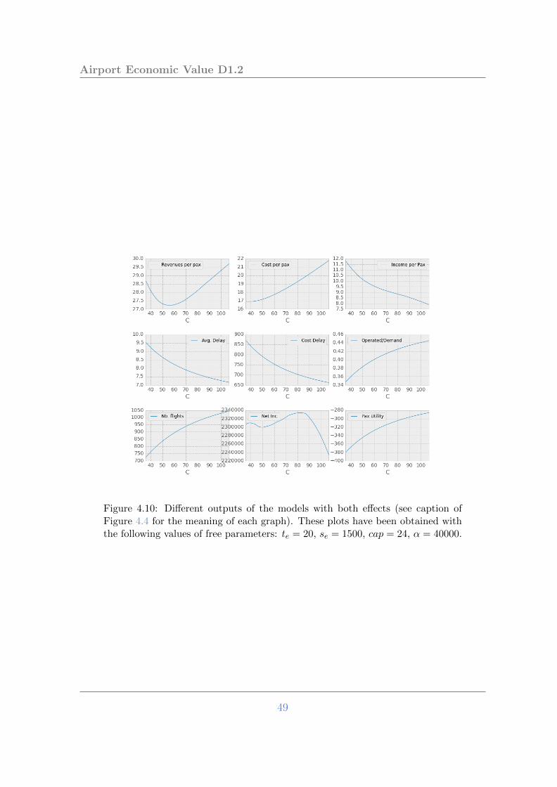
Airport Economic Value D1.2
Figure 4.10: Different outputs of the models with both effects (see caption ofFigure 4.4 for the meaning of each graph). These plots have been obtained withthe following values of free parameters: te = 20, se = 1500, cap = 24, α = 40000.
49

5 Conclusions
The work presented in this deliverable aimed at producing a new, highly data-drivenmodel able to give quantitative insights into the costs and benefits of extra capacityat an airport.
Technically, one of the most difficult tasks was the acquisition of data, and theirconsolidation. Indeed, it took a large amount of the effort just to acquire, clean,extrapolate and consolidate the data. Most of the sources have been used one way oranother, but two severe limitations have hindered the modelling process.
First, the lack of times series is a problem when one tries to build causal relation-ships, because correlations between different airports are typically less interpretablethan correlations in time for a single airport. Second, we were able to calibrate themodel only for a few airports, because there were several fields missing in the data formost of them. An analysis of more airports, especially for the cluster analysis, wouldhave allowed us to differentiate the model better, based on different types of airport.
A further main challenge was producing a model which can be calibrated, butwith enough realism to produce some quantitative outputs. Several tests have beenmade (we have produced around 15 versions of the model in total), but the final onewas simplified as much as possible to allow a full calibration: only one free parameterremains, which can be in fact roughly estimated, as shown in the sensitivity analysisC.
However, if the model is functionally simple, it embeds potentially complex be-haviour through the use of full distributions of delay and the corresponding expectedcosts. In fact, special attention has been applied to the impact of the non-linearity ofthe cost of delay, which can be taken into account only by using the full distributionof delays (in our case, a log-normal fit for each airport and each hour of the day).For the same reason, it was important for the model not to take for granted the basicdefinition of airport capacity, but to use a data-driven relationship, which, in essence,includes uncertainties regarding delays – with the consequence, for instance, that thecost of delay is not null even when the airport is operating below its theoretical ca-pacity threshold.
50

Airport Economic Value D1.2
Another advantage of a functional model is that it is very easy to modify andto include different relationships, either for further exploratory research or for moreairport-tailored results. This was performed in the more exploratory part of theresults, where we showed that complex interactions may arise between time spentshopping, passenger satisfaction, cost of capacity and satisfying demand – creatingdifferent types of curves for net income. This, is turn, will likely influence the futurechoices of the airport with respect to potential extensions of capacity.
However, it is clear that a functional model such as this one cannot capture all thecomplexity of reality. For instance, compared to some other simulation-based models,it is hard to introduce the feedback between different airports. Indeed, it is clear thatairlines make decisions at least on a two-airport basis (departure and arrival), and, insome cases, model route impacts at the full network level.
Hence, airlines will react differently to an increase in capacity at a departure air-port depending on the current state (and future, expected state) of the arrival airport.An increase or decrease in delay will thus meet different reactions, based on the delayat the other airport.
Another point not captured by our current model is the diversity of airlines. Notall of them react in the same way to the cost of delay, because they have differentbusiness models, different networks, different schedule buffers, etc. An operator suchas Ryanair, for instance, known to deploy large schedule buffers, may be more flexiblein terms of delay than some other operators, e.g. those operating connecting wavestructures at given airports (especially hubs).
The business models of the airports themselves will also attract different types ofoperator, and increases in capacity will have different impacts on them. Stated moregenerally, the heterogeneity of the different agents cannot be well captured by thistype of representative agents model.
Particular care has been taken regarding the choice of the right metrics and mech-anisms to consider in the model, constrained by the data available. For example,delay at an airport can obviously have many causes. Since it was desirable to capturethe delay directly caused by congestion, turnaround delay was focused upon. It wasalso important to treat aeronautical and non-aeronautical revenues separately, sincethey are two distinct sources that the airport can manipulate (to varying extents) tomaximise revenue. In particular, as seen in the exploratory analyses, airports mayhave a strong incentive to increase delay in some cases.
We have demonstrated that the model can be easily calibrated on real data andruns very well for the airports in our dataset. It produces reliable and realistic results.
51

Airport Economic Value D1.2
Some of them, in particular, are worth noting.
First, all the airports exhibit a maximum in net income as a function of capacity,if the marginal cost of operating extra capacity is sufficiently low (as illustrated inFigure 5.1). This threshold in the marginal cost is, however, rather different acrossairports, and only a few airports can sustain a high cost of capacity. As expected,these are the largest and most congested airports, which clearly need extra capacity.Moreover, we have shown that this threshold is roughly consistent with the airports’current operational cost of capacity, which means that they should be able to managethis growth, subject to the availability of investment.
Figure 5.1: Illustration of optimum capacity at an airport.
The exploratory results show that the picture can be significantly modified bythe introduction of variable, non-aeronautical revenues per passenger as illustrated inFigure 5.2. When tendencies to ‘shop more with more time’ and ‘shop better withincreased satisfaction’ are introduced, the net income can exhibit different maximaand minima. The direct consequence is that an airport would probably not be willing(or able) to invest sufficient capital to reach the global maximum, and is likely to be‘trapped’ in a local maximum. Since an increase in capacity is incremental (e.g. newrunway, new terminal), this may actually render it impractical for the airport to reachany maximum.
In future work, we hope to carry out a full calibration exercise on a specific airport.
52

Airport Economic Value D1.2
Figure 5.2: Complex landscape with local minima arising from the non-trivialnon-aeronautical revenues per passenger.
53

A Data analysis
In this annex, we give some detail about the data analysis performed in support ofthe modelling process.
A.1 Correlation structure
The full correlation matrix can be found in the next three pages. Table A.1 shows themeaning of each of the variables:
Abbreviation MeaningRegionE Share of European flightsAirlines Number of air operatorsRoutes Number of routes
Terminals Number of terminalsGates Number of gates
Runway number Number of runwaysTotal pax Total number of passengers
Delay per flight CODA turn-around delay per flightAvg pax/route Number of passengers per route
Net basic utility Net income minus aggregated cost of delayRunway usage Number of flight per runwayTerminal usage Number of flight per terminalAvg pax/flight Number of passengers per flight (load factor)
FLT DEP 1 Number of flightsturn delay Total turn-around delay
Capacity (hour) Maximum number of movements per hourCUI Capacity utilisation Index
Peak hour vol Peak hour volumeDom pax 2014 Number of domestic passengersInt pax 2014 Number of international passengers
Public ownership Share of public share in airportCHT% Percentage of charter flightsFSC% Percentage of full-service flightsLCC% Percentage of low-cost flightsREG% Percentage of regional flightsOTH% Percentage of other flights
TotalAeroRev13 Aeronautical RevenuesTotalNoneAeroRev13 Non-aeronautical revenues
TotalOpExp13 Operational expensesNetOpIncome13 Operational net income
Satisfaction Degree of passenger satisfaction at the airportCoordination Degree of coordination of the airport
Low Aggregated market share of regional and scheduled flightsHigh Aggregated market share of low-cost and charter flights
Table A.1
54
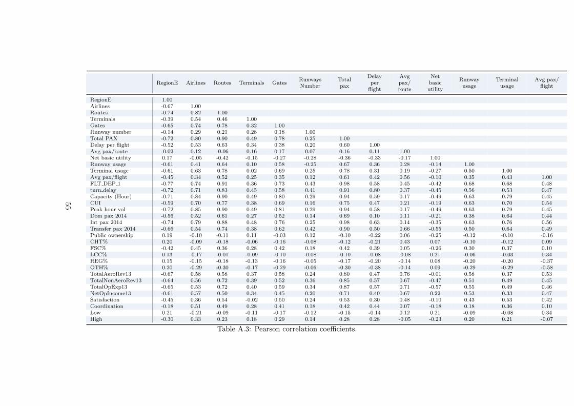
RegionE Airlines Routes Terminals GatesRunwaysNumber
Totalpax
Delayper
flight
Avgpax/route
Netbasicutility
Runwayusage
Terminalusage
Avg pax/flight
RegionE 1.00Airlines -0.67 1.00Routes -0.74 0.82 1.00Terminals -0.39 0.54 0.46 1.00Gates -0.65 0.74 0.78 0.32 1.00Runway number -0.14 0.29 0.21 0.28 0.18 1.00Total PAX -0.72 0.80 0.90 0.49 0.78 0.25 1.00Delay per flight -0.52 0.53 0.63 0.34 0.38 0.20 0.60 1.00Avg pax/route -0.02 0.12 -0.06 0.16 0.17 0.07 0.16 0.11 1.00Net basic utility 0.17 -0.05 -0.42 -0.15 -0.27 -0.28 -0.36 -0.33 -0.17 1.00Runway usage -0.61 0.41 0.64 0.10 0.58 -0.25 0.67 0.36 0.28 -0.14 1.00Terminal usage -0.61 0.63 0.78 0.02 0.69 0.25 0.78 0.31 0.19 -0.27 0.50 1.00Avg pax/flight -0.45 0.34 0.52 0.25 0.35 0.12 0.61 0.42 0.56 -0.10 0.35 0.43 1.00FLT DEP 1 -0.77 0.74 0.91 0.36 0.73 0.43 0.98 0.58 0.45 -0.42 0.68 0.68 0.48turn delay -0.72 0.71 0.83 0.45 0.58 0.41 0.91 0.80 0.37 -0.45 0.56 0.53 0.47Capacity (Hour) -0.71 0.84 0.90 0.49 0.80 0.29 0.94 0.59 0.17 -0.49 0.63 0.79 0.45CUI -0.59 0.70 0.77 0.38 0.69 0.16 0.75 0.47 0.21 -0.19 0.63 0.70 0.54Peak hour vol -0.72 0.85 0.90 0.49 0.81 0.29 0.94 0.58 0.17 -0.49 0.63 0.79 0.45Dom pax 2014 -0.56 0.52 0.61 0.27 0.52 0.14 0.69 0.10 0.11 -0.21 0.38 0.64 0.44Int pax 2014 -0.74 0.79 0.88 0.48 0.76 0.25 0.98 0.63 0.14 -0.35 0.63 0.76 0.56Transfer pax 2014 -0.66 0.54 0.74 0.38 0.62 0.42 0.90 0.50 0.66 -0.55 0.50 0.64 0.49Public ownership 0.19 -0.10 -0.11 0.11 -0.03 0.12 -0.10 -0.22 0.06 -0.25 -0.12 -0.10 -0.16CHT% 0.20 -0.09 -0.18 -0.06 -0.16 -0.08 -0.12 -0.21 0.43 0.07 -0.10 -0.12 0.09FSC% -0.42 0.45 0.36 0.28 0.42 0.18 0.42 0.39 0.05 -0.26 0.30 0.37 0.10LCC% 0.13 -0.17 -0.01 -0.09 -0.10 -0.08 -0.10 -0.08 -0.08 0.21 -0.06 -0.03 0.34REG% 0.15 -0.15 -0.18 -0.13 -0.16 -0.05 -0.17 -0.20 -0.14 0.08 -0.20 -0.20 -0.37OTH% 0.20 -0.29 -0.30 -0.17 -0.29 -0.06 -0.30 -0.38 -0.14 0.09 -0.29 -0.29 -0.58TotalAeroRev13 -0.67 0.58 0.58 0.37 0.58 0.24 0.80 0.47 0.76 -0.01 0.58 0.37 0.53TotalNonAeroRev13 -0.64 0.56 0.72 0.39 0.52 0.36 0.85 0.57 0.67 -0.47 0.51 0.49 0.45TotalOpExp13 -0.65 0.53 0.72 0.40 0.59 0.34 0.87 0.57 0.71 -0.57 0.55 0.49 0.46NetOpIncome13 -0.61 0.57 0.50 0.34 0.45 0.20 0.71 0.40 0.67 0.22 0.53 0.33 0.47Satisfaction -0.45 0.36 0.54 -0.02 0.50 0.24 0.53 0.30 0.48 -0.10 0.43 0.53 0.42Coordination -0.18 0.51 0.49 0.28 0.41 0.18 0.42 0.44 0.07 -0.18 0.18 0.36 0.10Low 0.21 -0.21 -0.09 -0.11 -0.17 -0.12 -0.15 -0.14 0.12 0.21 -0.09 -0.08 0.34High -0.30 0.33 0.23 0.18 0.29 0.14 0.28 0.28 -0.05 -0.23 0.20 0.21 -0.07
Table A.3: Pearson correlation coefficients.
55
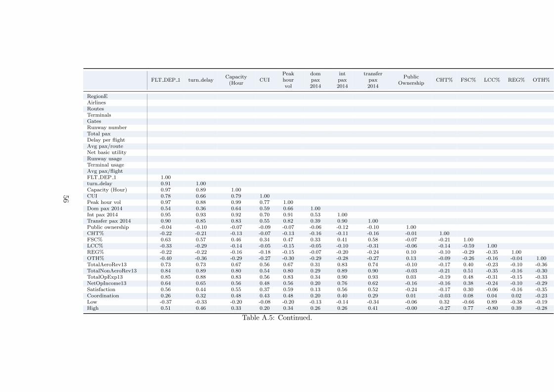
FLT DEP 1 turn delayCapacity
(HourCUI
Peakhourvol
dompax2014
intpax2014
transferpax2014
PublicOwnership
CHT% FSC% LCC% REG% OTH%
RegionEAirlinesRoutesTerminalsGatesRunway numberTotal paxDelay per flightAvg pax/routeNet basic utilityRunway usageTerminal usageAvg pax/flightFLT DEP 1 1.00turn delay 0.91 1.00Capacity (Hour) 0.97 0.89 1.00CUI 0.78 0.66 0.79 1.00Peak hour vol 0.97 0.88 0.99 0.77 1.00Dom pax 2014 0.54 0.36 0.64 0.59 0.66 1.00Int pax 2014 0.95 0.93 0.92 0.70 0.91 0.53 1.00Transfer pax 2014 0.90 0.85 0.83 0.55 0.82 0.39 0.90 1.00Public ownership -0.04 -0.10 -0.07 -0.09 -0.07 -0.06 -0.12 -0.10 1.00CHT% -0.22 -0.21 -0.13 -0.07 -0.13 -0.16 -0.11 -0.16 -0.01 1.00FSC% 0.63 0.57 0.46 0.34 0.47 0.33 0.41 0.58 -0.07 -0.21 1.00LCC% -0.33 -0.29 -0.14 -0.05 -0.15 -0.05 -0.10 -0.31 -0.06 -0.14 -0.59 1.00REG% -0.22 -0.22 -0.16 -0.18 -0.15 -0.07 -0.20 -0.24 0.10 -0.10 -0.29 -0.35 1.00OTH% -0.40 -0.36 -0.29 -0.27 -0.30 -0.29 -0.28 -0.27 0.13 -0.09 -0.26 -0.16 -0.04 1.00TotalAeroRev13 0.73 0.73 0.67 0.56 0.67 0.31 0.83 0.74 -0.10 -0.17 0.40 -0.23 -0.10 -0.36TotalNonAeroRev13 0.84 0.89 0.80 0.54 0.80 0.29 0.89 0.90 -0.03 -0.21 0.51 -0.35 -0.16 -0.30TotalOpExp13 0.85 0.88 0.83 0.56 0.83 0.34 0.90 0.93 0.03 -0.19 0.48 -0.31 -0.15 -0.33NetOpIncome13 0.64 0.65 0.56 0.48 0.56 0.20 0.76 0.62 -0.16 -0.16 0.38 -0.24 -0.10 -0.29Satisfaction 0.56 0.44 0.55 0.37 0.59 0.13 0.56 0.52 -0.24 -0.17 0.30 -0.06 -0.16 -0.35Coordination 0.26 0.32 0.48 0.43 0.48 0.20 0.40 0.29 0.01 -0.03 0.08 0.04 0.02 -0.23Low -0.37 -0.33 -0.20 -0.08 -0.20 -0.13 -0.14 -0.34 -0.06 0.32 -0.66 0.89 -0.38 -0.19High 0.51 0.46 0.33 0.20 0.34 0.26 0.26 0.41 -0.00 -0.27 0.77 -0.80 0.39 -0.28
Table A.5: Continued.
56

Airp
ort
Eco
nom
icV
alu
eD
1.2
TotalAeroRev13 TotalNonAeroRev13 TotalOpExp13 NetOpIncome13 Satisfaction coordination low high
RegionEAirlinesRoutesTerminalsGatesRunways NumberTotal paxDelay per flightAvg pax/routeNet basic utilityRunway usageTerminal usageAvg pax/flightFLT DEP 1turn delayCapacity (Hour)CUIPeak hour volDom pax 2014Int pax 2014Transfer pax 2014Public OwnershipCHT%FSC%LCC%REG%OTH%TotalAeroRev13 1.00TotalNonAeroRev13 0.77 1.00TotalOpExp13 0.80 0.97 1.00NetOpIncome13 0.94 0.74 0.69 1.00Satisfaction 0.50 0.51 0.49 0.47 1.00Coordination 0.30 0.26 0.31 0.20 0.17 1.00Low -0.26 -0.37 -0.34 -0.26 -0.12 0.02 1.00High 0.36 0.45 0.43 0.34 0.21 0.09 -0.89 1.00
Table A.7: Continued.
57

Airp
ort
Eco
nom
icV
alu
eD
1.2
Re-gionE
Air-lines Routes
Ter-mi-nals
Gates
Run-waysNum-ber
TotalPAX
Delayper
flight
Avgpax/route
NetBasicUtil-ity
Run-wayUs-age
Ter-minalUs-age
Avgpax/flight
RegionEAirlinesRoutesTerminalsGatesRunways NumberTotal PAXDelay per flightAvg pax/routeNet Basic Utility N/S N/SRunway UsageTerminal UsageAvg pax/flightFLT DEP 1 N/Sturn delay N/SCapacity (Hour)CUIPeak Hour Vol.dom pax 2014int pax 2014transfer pax 2014 N/SPublic OwnershipCHT% N/S N/SFSC%LCC% N/SREG% N/S N/S N/SOTH% N/S N/STotalAeroRev13TotalNonAeroRev13 N/STotalOpExp13NetOpIncome13Satisfaction N/Scoordination N/Slow N/Shigh
Table A.8: Significance statistical tests of correlation coefficients. All correlationsare significant with a 5% p-value, except where N/S is indicated.
58

Airp
ort
Eco
nom
icV
alu
eD
1.2
FLTDEP 1
turndelay
Ca-pac-ity
(Hour)
CUIPeakHourVol.
dompax2014
intpax2014
trans-ferpax2014
Pub-lic
Own-er-
ship
CHT% FSC% LCC% REG% OTH%
RegionEAirlinesRoutesTerminalsGatesRunways NumberTotal PAXDelay per flightAvg pax/routeNet Basic UtilityRunway UsageTerminal UsageAvg pax/flightFLT DEP 1turn delayCapacity (Hour)CUIPeak Hour Vol.dom pax 2014int pax 2014transfer pax 2014Public OwnershipCHT% N/SFSC%LCC% N/S N/SREG% N/S N/S N/S N/SOTH% N/S N/STotalAeroRev13TotalNonAeroRev13TotalOpExp13 N/SNetOpIncome13 N/SSatisfactioncoordinationlow N/S N/S N/Shigh
Table A.9: Continued.
59

Airp
ort
Eco
nom
icV
alu
eD
1.2
Tota-lAeroRev13
TotalNon-AeroRev13
TotalOp-Exp13
NetOpIn-come13
Satisfactioncoordina-
tionlow high
RegionEAirlinesRoutesTerminalsGatesRunways NumberTotal PAXDelay per flightAvg pax/routeNet Basic UtilityRunway UsageTerminal UsageAvg pax/flightFLT DEP 1turn delayCapacity (Hour)CUIPeak Hour Vol.dom pax 2014int pax 2014transfer pax 2014Public OwnershipCHT%FSC%LCC%REG%OTH%TotalAeroRev13TotalNonAeroRev13TotalOpExp13NetOpIncome13Satisfactioncoordinationlow N/Shigh
Table A.10: Continued.
60

Airport Economic Value D1.2
A.2 Clustering analysis
A.2.1 Methodology
There are many different ways of clustering data, each corresponding to the definitionof ‘clustering’. Several methods are routinely used in the literature but the specificchoice of method is always quite subjective. We decided to use a technique comingfrom network theory, based on modularity. If we consider a network with an adjacencymatrix A and a partition P of its nodes, the modularity is defined as:
Q =1
2m
∑C∈P
∑i,j∈C
(Aij − Pij), (A.1)
where Pij is the expected value of the adjacency matrix for the link i, j, and m is thetotal weights of the links. The modularity is typically a measure of how much thenodes are tightly linked to each other within the communities (clusters), with respectto how much they are linked with the rest of the network. The null model for thematrix is usually the one proposed by Newman and Girvan [57]: Pij = kikj/2m, whichcorresponds to a randomisation of the links, conserving the local strengths. There isthen the need to find the partition P of nodes which maximises the modularity, andfor this several algorithms exist. Here we use the Louvain method, which is veryefficient and widely used [58].
It is well known that the modularity suffers from a resolution issue, but there is aneasy and elegant way to circumvent this, by adding a scaling term to the null model’smatrix, i.e. Pij = γkikj/2m. If γ is high enough, typically very small communitiesare obtained (down to the size of one node each). A small value means on the otherhand that the partition maximising the modularity is the one where all nodes arein the same partition. In between, different levels of granularity of the system arespanned. If there is again a certain degree a subjectivity in the choice of the rightscale, this is strongly guided by the appearance of plateaus in the number of clusterswhen sweeping the scale – as shown below.
In order to use this method, the data must be organised in some type of network.A typical approach is to define a degree of similarity – or distance – between airports.Several choices are possible, but a common choice is to use the Euclidean distance onstandardised data, i.e. computing:
dij =
√∑k
(cki − ckj )2, (A.2)
where cki is the standardised value of the component k for airport i. The components
61

Airport Economic Value D1.2
are standardised as follows:
cki =c̃ki −minj c̃
kj
maxj c̃kj −minj c̃kj, (A.3)
where c̃kj is the initial, absolute value of the component. This means that all compo-nents span the interval [0, 1]. Note that different weights can also be put on differentcomponents, to better reflect either their importance or some prior knowledge of thedata.
In this study we use the components of the PCA for the distances between airports,instead of the initial variables, which reflect the natural organisation of the data.Moreover, we use the relative variance weights of each component in the Euclidean
distance, i.e. dij =√∑3
k=0wk(cki − ckj )2, where wk is the ratio of variance explained
with component k.In summary, we define a certain number of components (the same that we used for
the PCA), we build a network where each node is an airport and each pair of airportshas links of strength 1−dij, we sweep the parameter γ, and for each value we computethe best partition with the Louvain algorithm. In the following subsection we showthe result of the procedure.
A.2.2 Analysis of clusters
The first step is to check if there are some scales for which the system has a non-trivialnumber of clusters. Figure A.1 shows the existence of plateaus when sweeping thescaling parameter, more specifically a plateau with three communities and anotherone with four.
We then check that these plateaus actually correspond to stable partitions and not,for example, to a sequence of different partitions with the same number of clusters.We thus compute the normalised mutual information (NMI), which is a widely-usedmeasure of how alike two partitions are. We take several values of the γ within eachplateau, compute the NMI between each pair of the corresponding partitions, andaverage these results. The NMI score ranges between 0 and 1, where 0 indicates twototally unrelated partitions and 1 indicates that the partitions coincide exactly. Inother words, if the average NMI is 1, we conclude that the partition within each plateauis unique, which is indeed the case here. Overall, this indicates ‘good’ partitions,since they are stable in a finite range of the scaling parameters. Another check of therelevance of the partition can be made by disturbing the data with some noise andobserving whether the new partition is similar to the undisturbed one. The procedureapplied is as follows: we first choose a level of noise (for instance α = 1%) and foreach characteristic of each airport, we modify its value by a factor drawn randomly
62

Airport Economic Value D1.2
Figure A.1: Number of communities in the network of airports as a function ofthe scaling parameter. The presence of plateaus indicates the existence of naturalcluster structure at these scales.
between 1− α and 1 + α. We then recompute the partition (with the same value forγ) and compute the NMI between this partition and the initial one.
In Figure A.2, we show the NMI as a function of the level noise applied to the data.Clearly, for high levels of noise, the partitions are very different from the initial ones.The fact that there is a small plateau for low levels of noise is a further indicationthat the partition is quite robust. However, it is also clear that the clusters of theinitial partition do not differ greatly, since the NMI drops quite substantially after theplateau. Overall, we can conclude that this partition is robust statistically speaking,but that the characteristics of the airports tend to be continuous rather than harshlycategorical, which was as expected. Note also that a clustering analysis with manydifferent characteristics tends to produce these types of results, because of the varianceinduced by each additional component.
We then inspect the partitions themselves. In Table 3.2 we display the compositionof the 3-cluster partition. We firstly compare this partition with the 4-cluster partition(not shown), which is, in fact, very similar. The only difference is the presence of thenew cluster containing two airports, Copenhagen and Vienna, otherwise in clusternumber 2. Since the operational meaning of this small cluster is not obvious, we focusin this study on the 3-cluster partition.
63

Airport Economic Value D1.2
Figure A.2: Average Normalised Mutual Information (NMI) between partitionsbased on disturbed data and the original 3-clusters partition, as a function ofthe level of noise applied to the data. The error bars represent the standarddeviations over the 100 realisations of noise.
64
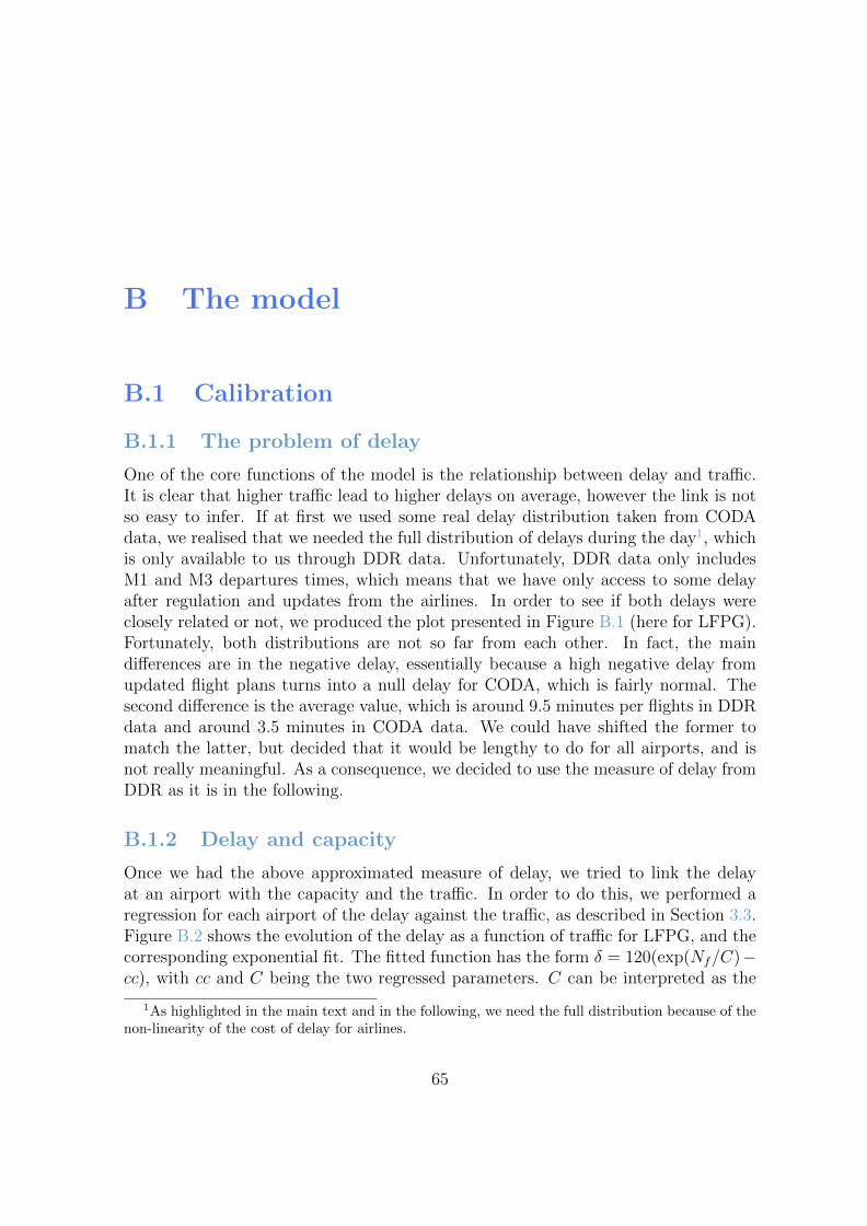
B The model
B.1 Calibration
B.1.1 The problem of delay
One of the core functions of the model is the relationship between delay and traffic.It is clear that higher traffic lead to higher delays on average, however the link is notso easy to infer. If at first we used some real delay distribution taken from CODAdata, we realised that we needed the full distribution of delays during the day1, whichis only available to us through DDR data. Unfortunately, DDR data only includesM1 and M3 departures times, which means that we have only access to some delayafter regulation and updates from the airlines. In order to see if both delays wereclosely related or not, we produced the plot presented in Figure B.1 (here for LFPG).Fortunately, both distributions are not so far from each other. In fact, the maindifferences are in the negative delay, essentially because a high negative delay fromupdated flight plans turns into a null delay for CODA, which is fairly normal. Thesecond difference is the average value, which is around 9.5 minutes per flights in DDRdata and around 3.5 minutes in CODA data. We could have shifted the former tomatch the latter, but decided that it would be lengthy to do for all airports, and isnot really meaningful. As a consequence, we decided to use the measure of delay fromDDR as it is in the following.
B.1.2 Delay and capacity
Once we had the above approximated measure of delay, we tried to link the delayat an airport with the capacity and the traffic. In order to do this, we performed aregression for each airport of the delay against the traffic, as described in Section 3.3.Figure B.2 shows the evolution of the delay as a function of traffic for LFPG, and thecorresponding exponential fit. The fitted function has the form δ = 120(exp(Nf/C)−cc), with cc and C being the two regressed parameters. C can be interpreted as the
1As highlighted in the main text and in the following, we need the full distribution because of thenon-linearity of the cost of delay for airlines.
65

Airport Economic Value D1.2
Figure B.1: Distribution of delays in CODA data (‘real’ delays) and DDR data forLFPG. The data has been truncated in the [−15, 120] region (following truncationfrom CODA data).
Figure B.2: Delay in seconds as a function of the traffic, for each hour of the day.The solid line is an exponential fit.
66

Airport Economic Value D1.2
capacity, since it is the typical traffic for which the delay significantly differs from itsoriginal value. cc is the delay when the traffic tends to zero, which is slightly negativefor most of the airports. Note that a linear fit is sometimes as good as an exponentialone, as shown below. Also the delays are still quite small (less than 10 minutes), sincethey are averaged over an hour. We will tackle the issue of very high delays for airlinesin the discussion that follows. Finally, note that the exact resolution for the fit is notobvious a priori, as our definition of capacity is now detached of any time period otherthan the averaging window. To tackle this problem, we performed for each airport amaximisation of the fit goodness by sweeping the resolution. Interestingly, the optimalresolution is not the same for every airport, which may reflect different operationalchoices.
Table B.1 shows the results of the fits for all the airports. For most of them, thefit is good, except for a couple (LIRF and EIDW). In order to use the capacity inthe model, we rescale it to have the equivalent hourly capacity (Chour in the table).Moreover, we decided to use the clusters found in the data analysis section in orderto get an average capacity. Indeed, it is quite clear that the fitted capacities fluctuatesignificantly within one cluster, so we are more confident in using an average one,since the airports in the same cluster should have similar operations. The last columnof the table show these averages, which are used in the model.
B.1.3 Cost of delay
The cost of delay is quite complex to assess, given the non-linearity of the cost asa a function of delay, and of the large distribution of delay. The basic cost perflight is shown in equation 3.1. However, the average delay in this equation cannotsimply be used in order to have the average cost. The easiest way to explain thisis to acknowledge that, even when the average delay is null, the average cost is not,because some flights have a positive delay (i.e. arrive early) whereas others have anegative delay and do not increase profits. As a result, a full distribution of delay wasconsidered.
In order to do this, and maintain a relatively simple model, we used a lognormalfit of the distribution of delay. Since for each hour of the day, the distribution is likelyto differ, we fitted the distribution of delay of each hour independently. Note that weused the whole month of data by aggregating each hour of each of the month. FigureB.3 shows an example of a fit for 9.00 am for LFPG. The fit is far from perfect, butroughly matches the data, and thus allows us to have a computation of the expected.Once we have fitted the probability of delay p(δ), the expected cost of delay c̄d is:
c̄d =
∫cd(δt)p(δt)d(δt)
By performing this procedure for each hour of the day, the total cost of delay for
67

Airport Economic Value D1.2
Res. Cres cc R2 Cluster Chour CcomEBBR 74 28.296911 -1.429895 0.709285 2 22.943441 29.393561EDDL 20 11.831204 -4.072900 0.617365 2 35.493611 29.393561EGCC 81 20.052234 0.451433 0.642084 2 14.853507 29.393561EIDW 94 71.311668 -3.025547 0.056397 2 45.518086 29.393561EKCH 18 13.500190 -3.626090 0.870522 2 45.000634 29.393561ENGM 46 26.990120 -0.837604 0.382568 2 35.204504 29.393561ESSA 50 25.630759 -0.869383 0.564417 2 30.756911 29.393561LOWW 29 16.600777 -1.437840 0.881326 2 34.346435 29.393561LPPT 57 15.721970 -3.438412 0.732810 2 16.549442 29.393561EDDF 35 21.956503 -2.452524 0.719974 1 37.639719 35.587806EDDM 24 29.398295 -3.367913 0.599480 1 73.495738 35.587806EGKK 46 15.507388 -1.136089 0.780133 1 20.227027 35.587806EGLL 29 13.882645 -0.810045 0.821380 1 28.722714 35.587806EHAM 46 38.471294 -2.787346 0.494721 1 50.179949 35.587806LEMD 46 22.940405 -2.734194 0.521661 1 29.922268 35.587806LFPG 47 32.313652 -1.483228 0.628944 1 41.251471 35.587806LIRF 91 438.107591 -3.775606 0.000976 1 288.862148 35.587806LSZH 70 30.412924 -2.072356 0.640382 1 26.068220 35.587806LTBA 84 17.896407 0.334670 0.817061 1 12.783148 35.587806EDDH 91 21.696123 -1.831217 0.522407 0 14.305136 17.813555EDDK 22 14.923674 -3.962501 0.327822 0 40.700929 17.813555EFHK 35 17.240393 -1.771224 0.660697 0 29.554959 17.813555EGBB 53 9.316811 -0.074231 0.886582 0 10.547333 17.813555EGSS 67 19.592047 -0.633787 0.544832 0 17.545117 17.813555EPWA 80 17.771291 -2.708330 0.656717 0 13.328468 17.813555LFMN 91 13.716757 -2.999108 0.840659 0 9.044016 17.813555LGAV 74 16.173872 -0.549414 0.902492 0 13.113950 17.813555LHBP 45 17.058659 -2.998551 0.496665 0 22.744879 17.813555LKPR 63 21.392047 -2.366516 0.685793 0 20.373378 17.813555LPPR 82 6.410945 -0.009339 0.322322 0 4.690935 17.813555
Table B.1: Results of the exponential fits of the delay against the traffic. Thefirst column is the resolution (in minutes) which gives the best fit. The secondand third columns are the corresponding values of the fitting parameters, and thefourth one is the corresponding coefficient of determination. The fifth column isthe cluster ownership (as found in the data analysis part). The sixth column isthe capacity recomputed for one hour, which is the resolution of the model. Thelast column features the average capacity in each cluster, which is taken as theinput by the model.
68

Airport Economic Value D1.2
Figure B.3: Histogram of the delays for LFPG at 9am, with a lognormal fit.
the airlines in one day is obtained by summing all the individual contributions. This‘corrected’ cost is indeed significantly different form the cost of the average delay, asshown on Figure B.4. Note that the correction itself depends on each airport, becausethe exact distribution of delay also does. This is the curve we directly use in themodel.
B.2 Model implementation
In this section, we present the specific equations that we used in the model. The firsttwo equations we used are relate to the delay-capacity relationship and the cost ofdelay, as presented previously. The other equations are detailed below.
B.2.1 Probability of operation
The core principle of the model is that the airline has a probability PA of operating aflight based on the expected cost of delays, which reads:
PA = 21
1 + ecd/s,
where cd is the expected cost of delay computed along the lines presented previously,and s is the smoothness parameter, discussed in the main text. This choice is moti-vated by the fact that the probability is linked to some form of utility function for
69

Airport Economic Value D1.2
Figure B.4: Correction of cost of delay for airline. The blue points are the costof the average delay, the violet ones are the expected costs taking into accountthe distribution of delay, and the solid red line is a quadratic fit of the latter.
the airline, taking into account other (strategic) parameters (as described above). Itallows us to have a smooth function which varies continuously between 0 and 1, andto have a risk aversion of the agent which can directly be linked to the parameters – henceforth referred to as the ‘smoothness’ of the decision. Indeed, when s issufficiently small, the airline takes harsh decisions, switching from operating to non-operating the route when the costs are driven high enough. Note that, in fact, weshould strictly be referring to net revenue contribution to the network, since airlineswill tolerate loss-making legs that have a net benefit to the system.
Moreover, we are able to introduce with this function an element of prospect theory,in the sense that the utility of the airline does not depend only on its revenues, butalso on a pre-determined level r0 (some kind of ‘anchoring’), by using cd + r0 insteadof simply cd. This parameter could include the direct revenues from the passengers(i.e prices of the tickets) and other costs linked to the operations. In the final versionof the model we decided not to use this parameter because it was hard to calibrateand did not bring interesting features (we would need to consider a full distribution ofr0 for this, which is beyond the scope of this research). Finally, this function mimicsstandard functions from prospect theory, since it is convex in the positive region (withrevenues greater than the value anchor) and concave otherwise.
70

Airport Economic Value D1.2
B.2.2 Implicit equation of delay
One important feature of the model is that it is auto-consistent for the delays, i.e. thedelays in the output are exactly the right level to match the actual traffic, which inturn sets the average delay through the delay-capacity relationship. In other words,setting a distribution of delays fixes the actual traffic through the use of probabilityPA, which in turn fixes the delay at each hour of the day through the capacity-delayrelationship. In order to solve this circular issue, we need to solve the implicit equation:
δ = 120 (exp(PA(δt)T/C)− cc) (B.1)
= 120
(exp
(2
1
1 + ecd(δt)/s
T
C
)− cc
), (B.2)
(B.3)
using the corrected function cd of the delay, as described above. T is the demand trafficfor this specific hour, i.e. the traffic extracted from data multiplied by β, as explainedin the main text. This equation is solved numerically using the Brent method. Theconvergence is assured by the fact that the right hand side is monotonically decreasingwith delay, and is strictly superior to 0 when δt = 0. So, there is always a solution,and only one, which is why we use a local optimisation algorithm.
B.2.3 The airport
Regarding the airport, we assume that its revenues come from aeronautical revenuesand non-aeronautical revenues. The former depends on the airport charges P and thepotential number of flights operated N , with:
rA,aero = PNPA.
The latter is directly linked to the number of passengers:
rA,non-aero = lfwNPA,
where lf is the average load factor and w is the average revenue coming from eachindividual passenger. In the final version of the model, the latter is a constant too.
Finally, we consider the expenses of the airport. Since we are interested in capacity-related costs, we choose a very simple form for the cost, linear with the extra capacity.The cost function reads:
cinf = α(C − Cinit) + cinit, (B.4)
where C − Cinit represents the increase in capacity desired by the airport, α is themarginal cost per unit of capacity, and cinit is the initial total expense of the airport– i.e. the expenses found in the data.
71

Airport Economic Value D1.2
In order to compare the consequences of the model for the different actors, we alsocompute a utility for the passengers:
up = −vδt, (B.5)
where v is the average value of time of the passengers. This is a very crude approxi-mation, and the computed utility has no intrinsic meaning, but is nevertheless usefulto compare different situations where delays are different and passengers are likely tobe satisfied at different levels. Note that we do not compare the results of the modelfor different airports and thus the satisfaction coming from the airport does not needto be estimated.
B.3 Exploratory analysis
This section shows some details of the results presented in 4.3.The equation we used to modify the non-aeronautical revenues of the airport is
the following:w(δt) = winit + wshop(δt) + wsat(δt).
It is composed of two components, plus the constant part winit, coming directly fromthe calibration. The first one is increasing with δt, and represents the tendency ofpeople to spend more when they have more time (‘more shopping time’). The secondcomponent is decreasing with δt and represents the tendency of people to spend morewhen their satisfaction is higher (‘better shopping time’). Since we assumed that thesecond component has an effect only when the delay is very high, whereas the firstone is present as soon as waiting increases, we use a quadratic and linear form forthese. The first reads:
wshop(δt) = teδt− δtinit
120winit,
and the second:
wsat(δt) =
{se(δt−δtinit
120
)2winit if δt < δtinit
−se(δt−δtinit
120
)2winit otherwise.
In these equations, δtinit represents the initial delay (the delay just after calibration).te and se are the weights given to each component, and are considered as free pa-rameters. Finally, we cap the value w, to avoid infinite revenues. The correspondingvariable is noted cap in the main text and is set to 24 euros to produce the results (tobe compared to the 17.7 euros after calibration).
As a result of this formulation, we are able to produce a non-trivial curve, shownin Figure B.5, which in turns contribute to the net income curve shown in the maintext.
72

Airport Economic Value D1.2
Figure B.5: Evolution of the function w with the delay, with δtinit = 9.5, winit =17.8, te = 15, and se = 1000.
73

C Sensitivity analysis
In this annex, we briefly show the results of a sensitivity analysis performed on acalibrated example of a large, European hub airport.
Since we have only one free parameter left in the model, we simply sweep it andsee how the calibrated parameters changes. In Figure C.1, we show the evolution ofthe average delay in the output and the revenues of the airlines (in fact, only the costof delay, negatively counted). These two outputs are the ones which are of interest,all others being fixed (e.g. the revenues per passengers) or trivially related to them(e.g. the utility of the passenger). Both quantities are changing with the smoothness,
Figure C.1: Evolution of the average delay (left) and revenues of airlines (right)in the calibrated model for various values of the smoothness parameter s.
but not drastically. For instance the delay goes from around 9 minutes per flight upto 11.7 minutes, which is a fairly narrow window, even though it is not negligible.It is worth noting that the actual value of the delay for the calibrated airport is 9.5minutes in the data, which means in fact that we could calibrate this last parameterto fit the average delay. We did not do it for technical reasons, but in the main text wechose s = 500, which gives a delay close to 9.5. We are thus confident that the resultspresented in the main text are sufficiently reliable with regard to the parameters.
74

Bibliography
[1] P. McCarthy, US airport costs and production technology a translog cost functionanalysis, Journal of Transport Economics and Policy 48 (3) (2014) 427–447.
[2] S. Gleave, Prepared for the UK CAA (2012).
[3] A. Cook, G. Tanner, European airline delay cost reference values, updated andextended values, version 4.1, https://www.eurocontrol.int/publications/
european-airline-delay-cost-reference-values (2015).
[4] CAA, Licence granted to heathrow airport limited by the civil aviation authorityunder section 15 of the civil aviation act 2012 on 13 february 2014 (2016).
[5] D. G. D. l’Aviation Civile, Economic regulation agreement between the govern-ment and Aeroports de Paris 2016-2020 (2015).
[6] T. D’Alfonso, C. Jiang, Y. Wan, Airport pricing, concession revenues and pas-senger types, Journal of Transport Economics and Policy (1) (2013) 71–89.
[7] E. Torres, J. S. Domı́nguez, L. Valdes, R. Aza, Passenger waiting time in an air-port and expenditure carried out in the commercial area, Journal of Air TransportManagement 11 (6) (2005) 363–367.
[8] M. Geuens, D. Vantomme, M. Brengman, Developing a typology of airport shop-pers, Tourism Management 25 (5) (2004) 615–622.
[9] J. Castillo-Manzano, Determinants of commercial revenues at airports: lessonslearned from Spanish regional airports, Tourism Management 31 (2010) 788–796.
[10] Y. Lin, C. Chen, Passengers’ shopping motivations and commercial activities atairports – the moderating effects of time pressure and impulse buying tendency,Tourism Management 36 (2013) 426–434.
[11] F. Fuerst, S. Gross, U. Klose, The sky is the limit? the determinants and con-straints of European airports’ commercial revenues, Journal of Air TransportManagement 17 (5) (2011) 278–283.
75

Airport Economic Value D1.2
[12] V. Fasone, L. Kofler, R. Scuderi, Business performance of airports: Non-aviationrevenues and their determinants (2016).
[13] S. Appold, J. Kasarda, The appropriate scale of us airport retail activities (2006).
[14] Y. Wan, C. Jiang, A. Zhang, Airport congestion pricing and terminal investment:Effects of terminal congestion, passenger types, and concessions, TransportationResearch Part B: Methodological 82 (2015) 91–113.
[15] Airports Council International, Does passenger satisfaction increase airport non-aeronautical revenue? A comprehensive assessment, research report (2016).
[16] CAA, Heathrow: Market power assessment (2012).
[17] R. Merkert, G. Assaf, Using DEA models to jointly estimate service quality per-ception and profitability – evidence from international airports, TransportationResearch Part A: Policy and Practice 75 (2015) 42–50.
[18] Y. Xiao, X. Fu, A. Zhang, Demand uncertainty and airport capacity choice,Transportation Research Part B: Methodological 57 (2013) 91–104.
[19] C. Barnhart, D. Fearing, A. Odoni, V. Vaze, Demand and capacity managementin air transportation, EURO Journal on Transportation and Logistics 1 (1-2)(2012) 135–155.
[20] J. Mart́ın, A. Voltes-Dorta, The dilemma between capacity expansions and multi-airport systems: Empirical evidence from the industry’s cost function, Trans-portation Research Part E: Logistics and Transportation Review 47 (3) (2011)382–389.
[21] J. Daniel, Benefit-cost analysis of airport infrastructure: the case of taxiways,Journal of Air Transport Management 8 (3) (2002) 149–164.
[22] J.-D. Jorge, G. de Rus, Cost-benefit analysis of investments in airport infrastruc-ture: a practical approach, Journal of Air Transport Management 10 (5) (2004)311–326.
[23] M. Gelhausen, P. Berster, D. Wilken, Do airport capacity constraints have aserious impact on the future development of air traffic?, Journal of Air TransportManagement 28 (2013) 3–13.
[24] P. Berster, M. Gelhausen, D. Wilken, Is increasing seat capacity common practiceof airlines at congested airports?, Journal of Air Transport Management 46 (2013)1–25.
76

Airport Economic Value D1.2
[25] A. Zhang, A. Czerny, Airports and airlines economics and policy: an interpretivereview of recent research, Economics of Transportation 1 (1) (2012) 15–34.
[26] IATA, Peak/off-peak charges.
[27] A. Czerny, A. Zhang, Airport congestion pricing and passenger types, Trans-portation Research Part B: Methodological 45 (3) (2011) 595–604.
[28] N. Adler, P. Forsyth, J. Mueller, H.-M. Niemeier, An economic assessment ofairport incentive regulation, Transport Policy 41 (2015) 5–15.
[29] M. Madas, K. Zografos, Airport capacity vs. demand: Mismatch or misman-agement?, Transportation Research Part A: Policy and Practice 42 (1) (2008)203–226.
[30] E. Verhoef, Congestion pricing, slot sales and slot trading in aviation, Trans-portation Research Part B: Methodological 44 (3) (2010) 320–329.
[31] B. Desart, D. Gillingwater, M. Janic, Capacity dynamics and the formulation ofthe airport capacity/stability paradox: a European perspective, Journal of AirTransport Management 16 (2) (2010) 81–85.
[32] A. Cook, G. Tanner, S. Anderson, Evaluating the true cost to airlines of oneminute of airborne or ground delay, University of Westminster, for EUROCON-TROL Performance Review Commission, Brussels, (2004).
[33] E. Gilbo, Airport capacity: Representation, estimation, optimization, IEEETransactions on Control Systems Technology (3) (1993) 144–154.
[34] FAA, Economic values for faa investment and regulatory decisions, a guide (2014).
[35] A. Zhang, Y. Zhang, Airport capacity and congestion pricing with both aeronauti-cal and commercial operations, Transportation Research Part B: Methodological44 (3) (2010) 404–413.
[36] International Transport Forum, Expanding airport capacity under constraints inlarge urban areas, discussion paper, (2013), p. 242.
[37] A. Montreal, Airport economics survey (2015).
[38] Z. Lei, A. Papatheodorou, E. Szivas, The effect of low-cost carriers on regionalairports’ revenue: evidence from the UK in Forsyth P., Gillen D., Muller J. andNiemeier H-M. (eds), Airport Competition: The European Experience, Alder-shot: Ashgate (2010).
77

Airport Economic Value D1.2
[39] V. Liebert, H. Niemeier, A survey of empirical research on the productivity andefficiency measurement of airports, J. Transp. Econ and Policy 47 (2) (2013)157–189.
[40] E. Pels, P. Nijkamp, P. Rietveld, Inefficiencies and scale economies of Europeanairport operations, Transportation Research Part E: Logistics and TransportationReview 39 (5) (2003) 341–361.
[41] J. Martin, A. Voltes-Dorta, International airports: economies of scale andmarginal costs 47 (1) (2010) 5–22.
[42] EC, Communication from the commission: Guidelines on state aid to airportsand airlines, Official Journal C99, 4 April (2014).
[43] CAA, Economic regulation at new runway capacity, cap 1279, london, caa (2015).
[44] K. Van Dender, J. Urban Econ. 62 (2007) 317–336.
[45] Y. Choo, Factors affecting aeronautical charges at major us airports, Transporta-tion Research Part A 62 (2014) 54–62.
[46] G. Bel, X. Fageda, Privatization, regulation and airport pricing: an empiricalanalysis for Europe, Journal of Regulatory Economics 37 (2) (2010) 142–161.
[47] V. Bilotkach, J. Clougherty, J. Mueller, Z. A, Regulation, privatization, and air-port charges: panel data evidence from European airports, Journal of RegulatoryEconomics 42 (1) (2012) 73–94.
[48] X. Fu, M. Lijesen, T. H. Oum, An analysis of airport pricing and regulation inthe presence of competition between full service airlines and low cost carriers,Journal of Transport Economics and Policy (JTEP) 40 (3) (2006) 425–447.
[49] CAA, Stansted: Market power assessment - annex 3 (2013).
[50] SEO, Impacts of expanding airport capacity on competition and connectivity, itf(2014).
[51] D. Starkie, G. Yarrow, Why airports can face price-elastic demands: Margins,lumpiness and leveraged passenger losses, International Transport Forum discus-sion paper 23 (2013).
[52] EUROCONTROL, Coda digest: All-causes delay and cancellations to air trans-port in Europe (2014).
78
Airport Economic Value D1.2
[53] European Commission, Regulation (ec) No 261/2004 of the European Parliamentand of the Council of 11 february 2004 establishing common rules on compen-sation and assistance to passengers in the event of denied boarding and of can-cellation or long delay of flights, and repealing Regulation (EEC) No 295/91, 17february 2004, 1-7 (2004).
[54] J.-O. Kim, C. Mueller, Factor Analysis – Statistical Methods and Practical Issues,SAGE Publications, Newbury Park, California, (1978).
[55] EUROCONTROL, Standard Inputs for EUROCONTROL Cost BenefitAnalysis (Edition Number: 7.0, November 2015), accessed on 28.06.2016,https://www.eurocontrol.int/sites/default/files/publication/files/
standard-input-for-eurocontrol-cost-benefit-analyses-2015.pdf
(2015).
[56] http://www.mathworks.com/products/compiler/mcr.
[57] M. Newman, M. Girvan, Finding and evaluating community structure in net-works, Phys Rev E 69 (2003) 026113.
[58] V. Blondel, J. Guillaume, R. Lambiotte, E. Lefebvre, Fast unfolding of commu-nities in large networks, JSTAT (2008) P10008.
79


![Building Value for Airport Communities - Trammell Crowmarketing.trammellcrow.com/Cynthia/Airport_Mini-Brochure[1].pdf · success for the airport and its tenants; • Adept at customizing](https://img.dokumen.tips/doc/110x75/5f02048f7e708231d4022b43/building-value-for-airport-communities-trammell-1pdf-success-for-the-airport.jpg)