Study on tangentially viewed 2D-SXR imaging system in the

九州大学学術情報リポジトリKyushu University Institutional Repository

Study on tangentially viewed 2D-SXR imagingsystem in the QUEST tokamak

黄, 燦斌

https://doi.org/10.15017/2534475

出版情報：九州大学, 2019, 博士（工学）, 課程博士バージョン：権利関係：

Study on tangentially viewed 2D-SXR imaging system in the QUEST tokamak

Doctoral Thesis

2019. 08

By

Huang Canbin (� ��)

Supervisor: HANADA Kazuaki (�� )

Advanced Energy Engineering Science

Interdisciplinary Graduate School of Engineering Sciences

Kyushu University, Japan

(i)

Abstract

This thesis reports investigations of soft x-ray (SXR) emission from the Q-shu

University experiments with Steady State Spherical Tokamak (QUEST) plasma using

a developed 2D-SXR imaging system. The system is a routine diagnostic on the

QUEST. The purpose is to develop a fast and high spatial resolved SXR imaging

system that can be applied to widely different plasma parameters in the various

operational scenarios. Since the intensity of SXR emission is related to plasma density,

temperature and impurity contents, the system in so-called imaging mode is used for

monitoring of fast changing plasma events, although the obtained images are the

line-integration of SXR emissivity at only center of QUEST chamber due to limited

field of view (FOV). By extrapolating the core signal to the edge, a tomography

reconstruction method—Abel inversion is expected to be performed to obtain the

emission profile with high accuracy.

In addition, owing to the fast time response of soft x-ray detector—microchannel

plate assembly and high framing rate of fast camera (up to 100 kHz), the system can

be used as soft x-ray photon counting device, which can provide the SXR energy

spectra and electron temperature measurement at the sacrifice of time resolution. It is

called the photon counting mode. The mode can be applied in only plasma being kept

constant during 1~2 seconds of sampling time. The photon counting mode was used

in the steady state operation with non-inductive current drive.

The thesis is organized as follows:

Chapter 1 is the introduction to SXR emission and SXR diagnostics on tokamak

devices. One type of regular SXR diagnostics is one-dimensional (1D)

scintillator-based arrays or diode-based arrays. With a wide coverage of the target

plasma, it can be used for tomographic reconstruction of two-dimensional (2D) soft

x-ray emissivity. Another type is direct 2D imaging of SXR emissivity, including SXR

camera or image intensifiers.

Chapter 2 is the introduction to the QUEST device and the 2D-SXR system.

QUEST is a medium sized spherical tokamak with all metal plasma facing wall (PFW)

and a temperature controllable “hot wall”. It is capable of generating long-duration

(ii)

discharges. One of the main goals of QUEST operation is to demonstrate the ability to

steady state operation. The schematic of 2D-SXR imaging system, including key

components of metallic filters, pinholes, MCP assembly and high-speed camera are

introduced in chapter 2. A mathematic gain model of the image intensifier is proposed

based on the characteristics of microchannel plate (MCP) and phosphor. The model is

consistent with bench test result of voltage scan on MCP and phosphor.

In chapter 3, the result of photon counting mode and SXR spectra are presented.

The algorithm of processing photon counting data is introduced, including the

integration of photons that occupy two or more pixels due to spreading of the finitely

sized electron clouds into neighboring pixels. Because energy calibration is not

available in 2D-SXR imaging system, a novel method of in-situ energy calibration

using Be filter transmission is proposed. It is applied in calculating SXR spectra and

electron temperature, and the error is evaluated.

In chapter 4, the result of imaging mode is presented. Spikes of SXR radiation

caused by slide-away electrons is detected by 2D-SXR imaging system. The temporal

waveform is consistent with other visible measurement on QUEST. With the

co-application of 8.2 and 28 GHz electron cyclotron waves (ECW), ~20 Hz

low-frequency plasma oscillation is observed. The imaging mode is used to study this

phenomenon in detail.

In summary, the innovative research works in this thesis focus on a compatible use of

the 2D SXR system such as photon counting mode and imaging mode. These

techniques were applied to QUEST plasmas and I could obtain the results of electron

temperature and slow plasma oscillation. Future work would include upgrading “bare”

MCP to KBr-coated MCP as well as improving the FOV of the system.

(iii)

��&'%��'��

�� !'%"�(�'�"!��

1.1.� ENERGY AND NUCLEAR FUSION��

1.2.� MAGNETIC CONFINEMENT FUSION AND TOKAMAK DEVICES��

1.3.� SOFT X-RAY RADIATION AND APPLICATION ON TOKAMAKS��

�� &�,'��)(-$(..'� '$,,$)(��

�� '*.+$-1�' �,.+ ' (-��

�� & �-+)(�- '* +�-.+ �' �,.+ ' (-��

1.4.� SOFT X-RAY DIAGNOSTICS ON TOKAMAKS��

�� ++�1,�,1,- '��

�� $'�"$("�,1,- '��

�� .&, �# $"#-��(�&12 +��

1.5.� MOTIVATION OF CURRENT RESEARCH��

�� '��&+%�� !��&,&'� �"!�$(�&'��

2.1.� THE QUEST SPHERICAL TOKAMAK��

2.2.� SCHEMATIC OF THE 2D-SXR SYSTEM��

�� %.,-��& �!$ &��)!�/$ 0��

�� $(#)& ,��(��!$&- +,��

�� ,, '�&1��

�� ,-��' +��

2.3.� GAIN MODEL OF 2D-SXR SYSTEM��

2.4.� BENCH TEST RESULTS��

� #�"'"!��"(!'�!��!��&+%�&#��'%( � ��&(%� �!'��

3.1.� PHOTON COUNTING MODE��

3.2.� ENERGY CALIBRATION USING BE FILTER��

3.3.� SXR SPECTRA AND TE CALCULATION��

3.4.� DISCUSSION��

�� !�� "��!��#��& �� "!�'"%�!��

4.1.� SLIDE-AWAY ELECTRONS DETECTION��

4.2.� PLASMA OSCILLATION��

(iv)

�� &( �%,��!��'��('(%��*"%��

�##�!��+��!)�%&�"!�"!��&+%�#%"��

��&'�"��#(��'�"!&��

%��%�!��&��

1

1. Introduction

1.1. Energy and nuclear fusion

In modern society, the demand for energy is kept increasing with the growth of

world population and economics. International Energy Agency (IEA) reported in “Key

world energy statistics 2018” that, in 2018, total primary energy supply was 13761

Mtoe or 1.6 ×10'()ℎ [1]. Fossil fuels are not renewable energy and they will be

exhausted within several tens or hundreds of years (petroleum is 30 years; natural gas is

30 years and coal are 500 years approximately) [2].

Among them, hydropower and other renewable energy only account for 10%, and

the nuclear fission energy is about 4%. The demand for nuclear energy decreased, in

part due to nuclear disasters (e.g. Three Mile Island in 1979, Chernobyl in 1986, and

Fukushima in 2011). Moreover, the nuclear waste from fission power plant remains a

big issue because of the high-level radioactive and long-lived fission products.

Fusion energy is very clean. Fusion energy is widely regarded as the ultimate

solution to the energy crisis. It is the energy source of the Sun and stars. As a source of

power, nuclear fusion is expected to have several theoretical advantages over fission.

These include reduced radioactivity in operation and little high-level nuclear waste,

ample fuel supplies, and increased safety.

The fusion reaction with the largest cross section is the D-T reaction:

D + T → He1 (3.5MeV) + n(14.1MeV) :1. 1;

If a nucleus of deuterium (D) fuses with a nucleus of tritium (T), an α-particle is

produced, and a neutron released. A total energy of 17.6 MeV is produced.

Naturally occurring tritium is extremely rare on Earth because it’s radioactive and

highly unstable. The half-life of tritium is about 12 years. For future nuclear fusion

reactors, tritium can be produced by neutron activation of lithium-6:

n + Li> → He1 (2.1MeV) + T(2.7MeV) :1. 2;

This is so called tritium breeding.

2

1.2. Magnetic confinement fusion and Tokamak devices

Due to the existence of Coulomb force, positive charged particles will be repelled

from each other. Sufficient kinetic energy of charged particles is required to overcome

the Coulomb force. Therefore, fusion processes require fuel and a confined

environment with sufficient temperature, pressure and confinement interval, to create a

plasma in which fusion can occur. It is feasible to heat the plasma to sufficient

temperature for fusion, such as using atomic bomb to ignite hydrogen bomb. Hydrogen

bomb is the exploitation of fusion energy in an uncontrolled method. However, the

question is how to confine the hot plasma and fusion reaction for energy outputs. This is

one of the major difficulties in nuclear fusion.

The Lawson criterion is a figure of merit showing the progress of performance in

nuclear fusion. It is suggested that the triple product of plasma electron density AB,

electron temperature C and the energy confinement time DE should reach a minimum

required value for net energy output of fusion. Fusion ignitron is the point at which a

nuclear fusion reaction becomes self-sustaining. For ignitron of deuterium–tritium, the

Lawson criterion gives [3]

ACDE ≥ 6 × 10G'keV s mK⁄ :1. 3;

This number has not yet been achieved in any reactor, although the latest generations of

machines have come close. JT-60U reported a maximum triple product of 1.5 ×

10G'keV s mK⁄ [4]. It is seen in Figure 1.1 that steady progress has been made in

fusion parameters over the past 50 years.

Magnetic confinement is one of two major branches of fusion energy research, the

other being inertial confinement fusion. The idea of magnetic confinement is to confine

the fusion fuel using high magnetic fields. The magnetic confinement devices consist

of Tokamaks, Stellarators, Z-pinch devices and so on. The largest magnetic

confinement device in the world is the International Thermonuclear Experimental

Reactor, or ITER in Acronym. ITER is currently under construction, and it is planned to

be finished in 2025 (www.iter.org). Figure 1.2 shows the schematic layout of the ITER

reactor. One of the major goals in ITER is to confine a D-T plasma with a-particle

self-heating to produce about 500 MW of fusion power with a ten-fold return on energy

(Q = 10).

3

Figure 1.1 Progress in fusion parameters over the past 50 years. Cited from [3]

Figure 1.2 Schematic layout of the ITER reactor experiment. Cited from [3]

4

1.3. Soft x-ray radiation and application on Tokamaks

1.3.1. Plasma continuum emission

There are several ways in which free electrons can emit radiation as well as

simply affecting its passage through the plasma via the refractive index. This radiation

proves to be of considerable value in diagnosing the plasma, especially since the

emission depends strongly upon the electron energy distribution, for example the

temperature of a Maxwellian plasma.

The plasma spectral emission consists of continuum emission and line emission.

The bremsstrahlung radiation occurs when a free electron makes a coulomb collision.

When the collision is with a positively charged particle such as an ion, the radiative

event can take one of two forms. It may be a free-free transition when the final state

of the electron is also free (total energy greater than zero) or it may be a free-bound

transition in which the electron is captured by the ion into a bound final state (total

energy less than zero). To distinguish these two types, the free-bound transitions are

often called recombination radiation.

Bremsstrahlung can be emitted over an exceptionally wide spectral range, from

the plasma frequency, usually in the microwave region, right up to the frequency whose

energy is of order the electron temperature or more, usually in the x-ray region. The

plasma continuum radiation is described in [5] using the following formula:

OPOℎQ ≈ CB

S' G⁄ T(CB, V)VBWWABG × exp Z−ℎQ\CB

] , (1.4)

where P is the radiated X-ray power, ℎQ is the SXR photon energy, CB, AB, and VBWW

are the electron temperature, electron density, and effective ion charge, respectively.

The factor T(CB, V) is the enhancement of the radiated power from recombination

radiation, which depends on the charge state distribution of the impurities V and

electron temperature. It is assumed in this formulation that the electrons are described

by a Maxwellian electron energy distribution function.

5

Figure 1.3 Bremsstrahlung spectrum and the recombination enhancement spectrum from a

0.17% oxygen contamination in ALCATOR A Tokamak. Cited from [6]

6

Figure 1.3 shows the Bremsstrahlung spectrum and the recombination

enhancement spectrum in ALCATOR A Tokamak [6]. To illustrate the contribution of

recombination to the hydrogenic bremsstrahlung spectrum, the enhanced spectrum has

been calculated for the case of a 0.17% oxygen contamination. The plasma temperature

is 870 eV and VBWW = 1.1. The effect of the oxygen is to produce a discontinuity at 870

eV (the ionization potential of the K shell in oxygen) and to enhance the spectrum in

ℎ^ > 870eV by about a factor of 2. If the ion species are identified, the enhancement

can provide a sensitive measurement of VBWW.

1.3.2. Impurity measurement

Since the continuum radiation is related to impurity contents in plasma, it can be

applied for impurity measurement. Impurity control is important in plasma operation as

they play an important role in the plasma performance. The presence of impurities in a

tokamak plasma affects the particle collisionality, the electrical resistivity and the

transport properties as well as diluting the fuel density and reducing the thermal

confinement through radiation losses. Moreover, control of plasma-wall interactions

(PWI) is one of the key issues for steady state plasma operation. In modern tokamaks,

wall conditioning is necessary to reduce the impurity contents and create a clean

background for the plasma. On the EAST tokamak, real-time wall conditioning with

lithium powder injection is applied in long-pulse (> 30a) H-mode plasmas [7].

The average plasma ion charge, or “effective Z”, is given by:

VBWW =∑AcVcG

∑ AcVc=∑AcVcG

AB(1.5)

where AB is the electron density and Ad is the density of ions of charge state Vc in the

plasma. is required by quasi-neutrality in electrical charge in plasma

VBWW profile can be measured from bremsstrahlung imaging in the MAST

spherical tokamak [8]. The electron temperature and density profiles are required to

determine the VBWW profile. A system measures bremsstrahlung radiation in the range

of visible to near infrared radiation to avoid the complicating contribution from the

recombination continuum. The most important precaution in performing the

VBWWmeasurement in the visible is to ensure that the intensity is measured in a spectral

7

region free from strong impurity line radiation. This is often a difficult requirement to

meet.

On QUEST tokamak, the main impurities are ionized carbon and oxygen

impurities [9]. The enhancement factor arises predominantly from ionized carbon and

oxygen impurities.

1.3.3. Electron temperature measurement

For ℎ^ ≥ C, the emission from both free-free and free-bound transitions has a

strong (exponential) dependence upon the temperature (see Equation 1.4 and Figure

1.1). In this energy range, the main diagnostic with the emission is as a measurement of

electron temperature. Usually the instrument used to obtain the Bremsstrahlung

spectrum is an X-ray pulse height analyzer (PHA), as introduced in Section 1.4.3.

In our system, we use the photon counting mode of 2D-SXR imaging system to

obtain the Bremsstrahlung spectrum. The spatial resolution is better than typical PHA

system.

8

1.4. Soft X-ray diagnostics on Tokamaks

Soft x-ray diagnostics are common in low and high temperature plasma research,

and can provide information on plasma temperature, density, and impurity content.

Here we introduce different types of regular SXR diagnostics, as well as their

advantages and disadvantages.

1.4.1. 1D SXR arrays system

One-dimensional (1D) SXR arrays are commonly used for SXR imaging system.

They are often poloidally distributed around the plasma cross section, viewing the

plasma through identical filters to provide a tomographic reconstruction of the x-ray

emission. Two types of detectors can be used in the SXR arrays – indirect detector of

scintillator that convert x-rays to visible lights, or direct detector of semiconductors that

directly convert x-ray photons to electrical charge. The former is called

scintillator-based arrays (examples in [5]).The latter is called diode-based arrays

(examples in [10, 11]).

Diode-based system over the optical, scintillator-based arrays has an advantage of

wide energy dynamic range, higher sensitivity and signal-to-noise ratio (SNR) even for

low energy, calibration stability [11]. These factors enable SXR detection in lower

energy and allows to use for the multi-energy soft x-ray (ME-SXR) measurement from

the plasma core to the lower temperature edge region. On the other hand, the optical,

scintillator-based arrays have better resistance to the noise signal introduced by neutron

bombardment and electromagnetic pickup. Other advantages include that it can create a

large detector area with a relatively inexpensive phosphor deposition on

medium-to-large (5–15 cm) fiber optic windows. It can provide a portable, compact

design with ultrahigh vacuum (UHV) and high-temperature bakeout compatibility [12].

9

Figure 1.4 Tangential geometry for 48-channel the multicolor scintillator-based

optical soft x-ray array diagnostic on NSTX. Cited from [5]

Figure 1.4 show a “multicolor” scintillator-based optical soft x-ray on NSTX

Tokamak [5]. It has been developed for time- and space-resolved measurements of the

electron temperature [CB(f, g)] profiles in magnetically confined fusion plasmas.

Potentially, it can also measure profiles of the electron and impurity density product

[ABAi(f, g)] as well. Here the word “multicolor” denotes the device uses Be filter of

three different thickness (10-μm, 100-μm and 300-μm) to provide energy

discrimination. This device consists of three arrays of tangential sight lines that view

the same plasma volume at the machine’s midplane, as shown in Figure 1.4. Each array

observes the plasma through a separate pinhole and filter, with the capability of

providing time- and space resolved measurements of the radial SXR emissivity with

rough energy discrimination. To be noted, the device cannot provide the absolute

electron temperature profile alone. By calculating the ratio of the SXR emissivity

measured over two or more energy ranges from different Be filters, high time resolution

profiles of relative change in electron temperature [∆CB(f, g)] can be obtained. In

conjunction with the absolute measurements produced by a multipoint Thomson

scattering (MPTS) system, fast evolution of the electron temperature profile between

the MPTS sampling times can be obtained.

10

1.4.2. 2D SXR imaging system

Soft x-ray tomographic reconstruction methods are used in 1D SXR arrays system

to reconstruct plasma image for magnetohydrodynamic (MHD) studies. However, the

spatial resolution is limited by the channel number of soft x-ray arrays. Moreover, a

large number of equally spaced detectors surrounding the plasma is needed to obtain a

reliable reconstruction. Due to limited access and scarcity of ports, this is not always

possible.

Direct 2D SXR imaging with high spatial and time resolutions has recently been

made possible through the use of charge coupled device (CCD) cameras sensitive to

SXR [13] or image intensifiers comprising a microchannel plate (MCP) detector and a

phosphor screen coupled to a high-speed video camera [14, 15]. These systems can

measure two dimensional SXR images directly with high spatial and time resolution.

Figure 1.5 Top view of experimental setup for soft x-ray CCD camera system in compact helical

system (CHS). Cited from [13]

11

Figure 1.5 shows the schematic of soft x-ray charge coupled device (CCD) camera

system in compact helical system (CHS) [13]. The amount of charge in each pixel of

the CCD created by the individual x-ray photon is proportional to the energy of the x

ray. Therefore, it can be used as a photon counting device with good spatial resolution.

The flux of soft x rays can be adjusted by changing the size of the pinhole (0.03, 0.1,

and 0.3 mm). The energy range measured can be selected by rotating a filter disk and

changing six Be filters, with different thicknesses of (10, 30, 70, 140, 300, and 800 μm).

The x-ray energy calibration of the CCD camera was done using Fe Ka line (6.4 keV)

and Fe Kb line (7.06 keV) from a Fe target x-ray sources. The system can measure a

two-dimensional profile of energy spectra of x-ray emission and electron temperature

for magnetically confined plasmas.

Compared with SXR cameras, the image intensifier of an MCP detector can

measure SXR signals with higher gain, enabling their use in low-density plasmas.

Figure 1.6 shows the schematic of the high-speed vacuum ultraviolet (VUV) imaging

system for the Experimental Advanced Superconducting (EAST) Tokamak [15]. Its

key optics is composed of an inverse type of Schwarzschild telescope made of a set of

Mo/Si multilayer mirrors, a micro-channel plate (MCP) equipped with a P47 phosphor

screen and a high-speed camera with CMOS sensors. These multilayer mirrors can

selectively measure photons with 13.5 nm wavelength, which comes from impurity line

emission of interests on EAST. It is noted that this system is optimized for imaging of

mono-energy VUV photons. In contrast with normal pinhole structure, the X-ray

mirrors allow much more photons to be detected (10k times higher than in a pinhole of

100 μm in diameters.). Unlike the SXR camera in CHS (see Figure 1.5), the VUV

imaging system is not capable of photon counting measurement. The gain of the MCP

is about 10l with an operation voltage of 2.4 kV.

12

Figure 1.6 Schematic of the optics of the high-speed VUV imaging system on the EAST. MCP

equipped with a P47 phosphor screen is used as the image intensifier. Cited from [15].

1.4.3. Pulse height analyzer

As a conventional soft x-ray diagnostic, the pulse height Analyzer (PHA) has been

well developed to measure electron temperature as well as the concentration of high-z

impurity from the x-ray energy spectra [16, 17]. In prototype PHA system, silicon or

germanium doped with lithium (Si(Li) or Ge(Li)) semiconductor detectors are used

[18]. However, they need to be cooled with liquid nitrogen. Now Silicon drift detectors

(SDDs) is widely used in PHA system. It is cost-effective with higher performance. It

allows for the use of Peltier cooling instead of the traditional liquid nitrogen. The

advantage of PHA system is that they have high time and energy resolution, and high

signal-noise ratio. The disadvantage of PHA systems is that they have a relatively small

number of spatial channels (limited by the number of detectors) and poor spatial

resolution.

Figure 1.7 shows the schematic of PHA system on the J-TEXT tokamak [17]. The

detector system consists of detectors, pre-amplifiers, main amplifiers, and

multi-channel analyzers (MCA), as illustrated in Figure 1.7 (b). The Silicon Drift

Detectors (SDDs) have high performance, such as high-count rate (~100 kHz) with

almost no dead time, high quantum efficiency (mn > 0.9 over the range of 2-12 keV)

and high energy resolution (150 eV at 5.9 keV). A DC voltage supply and cooling

system are required for the SDDs operation. The system uses Fe and Cu standard

radiation sources for the energy calibration.

Figure 1.8 shows a typical soft X-ray spectrum acquired by the J-TEXT PHA

13

system. Only the relative spectral intensity is plotted (on a log scale) because the great

advantage of this method is that it requires only the gradient of the spectrum, not its

absolute intensity, to give the electron temperature. The electron temperature of 770 eV

can be derived directly from the slope of the semi-log plot of the spectrum using linear

regression analysis.

Figure 1.7 (a) The schematic of the J-TEXT PHA system and (b) the flow chart of detection part

of the system. Cited from [17].

14

Figure 1.8 A typical semi-log spectrum obtained by J-TEXT PHA system which gives an

electron temperature of ~770 eV. Here the Y-axis is the logarithm of radiation intensity. Cited

from [17].

15

1.5. Motivation of current research

Regular SXR diagnostics have been briefly introduced in Section 1.4. They all

have their own disadvantages and are considered not suitable for applying on the

QUEST tokamak. 1D SXR arrays system measures the SXR emissivity along the arrays.

It has wide coverage but poor spatial resolution (limited by number of channels). The

pulse height analyzer is capable of photon counting and SXR spectra measurement.

The spatial resolution is limited by the number of SSD detectors.

2D imaging systems have better spatial resolution than 1D arrays system. They

can provide 2D images, which allows study of plasma shape evolution and spatial

movement. For SXR camera-based imaging system, it is small and compact. The CCD

camera sensitive to SXR is used as the SXR detector and image readout device.

However, the image gain is usually limited as no image intensifier is used. This is not

suitable for measuring low density plasma on the QUEST tokamak.

In this thesis, the author introduces a tangentially viewing 2D SXR imaging

system developed for the QUEST tokamak. It used an image intensifier that consists of

a two-stage MCP, P46 phosphor and fast camera as image readout device. It has very

high gain (1 × 10(), thus can be applied for QUEST plasma with low density and low

heating power. It is flexible to change the gain by changing the applied voltage on MCP

and phosphor; thus, the system can be easily applied for different operational scenarios.

Similar image intensifier was used in the VUV imaging system on EAST (see Figure

1.6). In contrast, our system on QUEST is optimized for SXR imaging, and is capable

of measuring the SXR spectra.

Two operational modes have been developed --- photon counting mode and

imaging mode. Photon counting mode is capable of photon counting and calculating

SXR spectra in long discharges, when plasma parameter should be constant during data

sampling time. While HXR spectra can be obtained by the HXR system available on

QUEST [19], photon counting mode of 2D-SXR is the only method to obtain reliable

SXR spectra in energy range of 1~8 keV. Compared with pulse height analyzer, the

position of photons is also recorded by the system, because of high spatial resolution of

MCP detector. Thus, the spatial resolution of SXR spectra can be increased by dividing

data into more spatial channels at the cost of lower count rate.

16

On the other hand, imaging mode can provide high spatial and temporal resolution

images of SXR emissivity viewing at the center of plasma, which reveals information

on plasma density, temperature and impurity content. The spatial and temporal

resolution of the system is limited by the read-out device of fast camera. Compared

with SXR cameras, the performance of system can be upgraded by simply changing a

better camera. Imaging mode can be applied to monitor fast changing plasma events, as

seen in the two examples (impurity radiation and plasma oscillation phenomenon)

discussed in Chapter 4.

Since the gain of MCP assembly changed with different applied voltage, it is

difficult to apply convention energy calibration using X-ray sources. Therefore, we

developed an in-situ method of energy calibration using the transmission of Be filter, as

described in Section 3.2. The method is useful for both photon counting mode and

imaging mode. The calibrated values in the photon counting mode can be used to

determine the absolute value of SXR radiation energy. And the energy-calibration

relation and the calibrated values can be used for imaging mode that the signal is piled

up, as long as the applied voltage on MCP and phosphor is the same. In this way, we can

get the absolute value of SXR emission energy, which can then be used to estimate the

radiation loss from the plasma. This is another merit of the system.

In the appendix, the author discussed the efforts of developing an algorithm to

perform Abel inversion on mid-plane profile of SXR images, when the edge and center

profile is unknown (only the center of QUEST chamber can be observed).

17

2. The 2D-SXR imaging system on QUEST

2.1. The QUEST Spherical Tokamak

The Q-shu University experiments with Steady State Spherical Tokamak

(QUEST) is a medium size Spherical Tokamak (ST) device in Kyushu University,

which starts first plasma experiment at Oct. 2008 [20, 21]. A photography of QUEST is

shown in Figure 2.1. The main purpose of QUEST is to study the generation of high p

plasma and current drive, as well as the steady state operation (SSO) and recycling

control in Spherical Tokamak. Table 2.1 shows the main parameters of the QUEST

tokamak. The electron density is about 10'>~10'lrSK, 100 times lower than other

big devices.

Table 2.1 The main parameters of QUEST

Major radius 0.64 m Minor radius 0.4 m

Radius of outer limiter 1.32 m Radius of inner limiter 0.22 m

Outer diameter of the

vacuum chamber

2.74 m Inner diameter of the

vacuum chamber

0.44 m

Aspect ratio 1.7 Height of the vacuum

chamber

2.8 m

Maximum toroidal

magnetic field at major

radius

0.25 T (steady state)

0.5 T (pulse)

Maximum plasma

current

100 kA

�Obtained�

300kA

(Designed)

Number of toroidal coils 16 Number of poloidal coils 11

Electron density AB 10'>~10'lrSK

18

Particle recycling and heat control are important issues for the steady-state

operation. QUEST is capable of performing steady state operations with all-metal

plasma facing walls (PFWs) [21, 22]. Water-cooled hot walls were installed on the top

and bottom conical portions of the vacuum vessel. They are able to control its

temperature in the range of 373K-737K for the purpose of particle flux control. The

body of plasma facing components PFCs including vessel chamber, center stack cover,

hot wall and divertor plates is made of type 316-L stainless steel. The surface of PFCs is

coated with a layer of 0.1 mm-thick atmospheric plasma-sprayed tungsten (APS-W). A

record of long discharge lasting 1h 55mins with well-controlled wall temperatures

using the hot wall [21] and proper Hα level feedback control was achieved on QUEST

[22].

Two 8.2 GHz with power up to 200 kW and a 28 GHz electron cyclotron wave

Figure 2.1 Left figure: photograph of the QUEST tokamak. Right figure: schematic diagram

of poloidal field (PF) coils and plasma facing components (PFCs) of the QUEST tokamak.

The body of PFCs is made of type 336-L stainless steel and its surface is coated with a layer

of 0.1 mm-thick atmospheric plasma-sprayed tungsten (APS-W).

19

(ECW) system are used for current start-up and current drive[20, 23]. Another 2.45

GHz system with power up to 50 kW is used for low power discharging such as during

cleaning of the chamber wall [20]. Fully non-inductive second (2nd) harmonic electron

cyclotron (EC) plasma current ramp-up was demonstrated with a newly developed 28

GHz system in the QUEST spherical tokamak [23]. A center solenoid (CS) coil is used

for Ohmic heating [21].

20

2.2. Schematic of the 2D-SXR system

2.2.1. Adjustable field of view (FOV)

The 2D-SXR imaging system was installed at a tangential port on QUEST. Due to

the limitation of current system, it can only watch the core region of QUEST plasma

and some of the ECW harmonic resonance layers. When st is fixed at 0.13T at major

radius(f = 0.64m), the fundamental and second harmonic resonance layers of 8.2

GHz ECW are located at fuBv' = 0.29m and fuBvG = 0.58m, respectively. Figure

2.2 (a) shows 3-D field of view (FOV) of the system. The viewing area is a range of

36-cm circle at the poloidal section of QUEST, which is changeable at radial direction

by moving the rear end of the system. Figure 2.2 (b) shows the typical FOV at imaging

mode (f = 0.26– 0.62m) and photon counting mode (f = 0.48– 0.84m) in this

paper.

Figure 2.2 Schematic of FOV of the tangential SXR imaging system on QUEST. (a) 3-D view;

(b) poloidal section with movable FOV (red color circle in imaging mode and green color circle

in photon counting mode). Fundamental and second harmonic resonance layers of 8.2 GHz

ECW at st = 0.13T are denoted by red and green lines. Cited from [24, 25]

21

2.2.2. Pinholes and filters

Figure 2.3 Schematic of the SXR imaging system on QUEST. A 25-μm-thick Be filter mounted

on 1 and 6-mm pinhole plates is displayed; another set of 2- and 4-mm pinhole plates is also

available. Cited from [24, 25]

Figure 2.3 shows a schematic of the QUEST 2D-SXR diagnostics. The incoming

SXR flux can be adjusted by changing the size of the pinhole (between 1, 2, 4, and 6

mm) using a slider. Unfortunately, the slider must be changed manually (see the

photography in Figure 2.4). It means the pinhole size and filter can only be changed at

the interval of two discharges. The pinhole plate is made of 1mm SUS304 stainless

steel. Figure 2.5 shows the transmission rate of the pinhole plate. It is seen that 1mm

SUS304L (stainless steel type 304L) stainless steel can block soft x-ray less than 20

keV. However, the pinhole plate is not enough to shield the hard X-rays produced by

energetic electrons in non-inductive current drive on QUEST [26]. Therefore, we used

a 30-mm-thick tungsten mask with a V-shaped hole mounted at the front of the pinhole

plate as an additional shield against hard X-rays. It is noted that the hard X-ray

shielding is not perfect. Some of hard X-rays can still be recorded in the images. If they

are within the MCP viewing area, it is difficult to remove them.

QUESTPlasma

Al filter5 µm Vacuum

Pump

Visiblelight

Camera viewer

MCP

P46 phosphor

Gate Valve

Soft x-ray

Be filter25 µm

Magnetic shield

Gate Valve

Shutter

Pinhole slider

V-shape W Mask

22

Figure 2.4 Photograph of 2D-SXR system on QUEST.

23

Figure 2.5 Transmission data pinhole plate made of 1mm stainless steel (SUS304). (a) In

soft x-ray energy range of 0~10 keV. (b) In soft x-ray energy range of 10~30 keV. The

absorption edge around 6 keV comes from K-edge of Cr (5.99 keV).

The filters are important in SXR diagnostics. By choosing different filters we can

select the energy window of measurement. If several filters can be used at the same

time, a good energy resolution can be obtained by subtracting the intensity of different

filters. In our system, we use a 5-μm-thick Al filter mounted on a shutter to prevent

visible and ultraviolet (UV) photons from entering the imaging system. The photograph

of the shutter and Al filter is shown in Figure 2.6. Due to limited number of pinholes,

we use a 25-μm-thick Be filter mounted on the plate to cover the middle two of the four

pinholes. In this way we can compare two similar discharges with and without Be filter

at the same pinhole size. This method is applied in the energy calibration in photon

counting mode. The details of the energy calibration are described in Section 3.2. The

photograph of the 2-4 mm and 1-6 mm pinhole plates and Be filter is shown in Figure

2.7.

10 15 20 25 30Photon Energy (keV)

0

0.5

1

1.5

2

2.5

Tran

smis

sion

10-30 2 4 6 8 10

Photon Energy (keV)0

0.5

1

1.5

2

2.5

Tran

smis

sion

10-28 1mm SUS304 pinhole plate

(a)

(b)

24

Figure 2.6 Photograph of (a) 5-μm-thick Al filter mounted on an openable shutter. (b)

Half-open shutter.

Figure 2.7 Photograph of (a) back and front side of 2mm and 4mm pinhole plates. (b) back and

front side of 1mm and 6mm pinhole plates. 25-μm-thick Be filter is attached to the middle two

of the four pinholes.

25

Figure 2.8 Filter transmission data in soft x-ray energy range (a) the transmission of

5 μm Al filter, 25 μm Be filter and two filters together. (b) the transmission of 0.4 μm

Al filter and 5 μm Al filter.

Besides, we have another set of 0.4-μm Al filter mounted on the pinhole plate that

can be used in the imaging mode. This will allow soft x-ray detection above ~300 eV.

The filter transmission data of these filters are shown in Figure 2.8.

0 1 2 3 4 5 6 7 8 9 10Photon Energy (keV)

0

0.2

0.4

0.6

0.8

1

Tran

smis

sion

Al 5 mBe 25 mAl+Be

0 1 2 3 4 5Photon Energy (keV)

0

0.2

0.4

0.6

0.8

1

Tran

smis

sion

Al 0.4 mAl 5 m

(a)

(b)

26

2.2.3. MCP assembly

The core component of the SXR imaging system is a chevron detector assembly

from PHOTONIS USA, INC. It contains two Imaging Quality Advanced Performance

Long-LifeTM Microchannel Plates (MCP) and a fiberoptic phosphor screen with P46

phosphor mounted to a 6.0" vacuum flange. Figure 2.9 shows the photograph of the

MCP assembly. The green area denotes the phosphor screen. The fiberoptic is frit

sealed into the flange to form a vacuum seal that is tight to a leak rate of 10S'xcc/sec of helium. The detector assembly is mounted in stainless steel hardware which is

bake-able to 300°C. The specification of the MCP assembly is shown in Table 2.2.

MCP is composed of many miniature electron multipliers (or channels) parallel to

each other, as shown in Figure 2.10. MCP can amplify the electron signal via electron

cascade process inside a single channel. The spacing of channels determines the spatial

resolution of MCP. In the current MCP, the channel size is 10 μm and the

center-to-center spacing of channels is 12 μm, which is very fine structure. The time

response of MCP is very fast (< 1ns) [27].

Figure 2.9 Photograph of the MCP assembly mounted to 6.0" vacuum flange. Left figure:

front side. Right figure: back side. The green area is the phosphor screen.

27

Figure 2.10 Left: Micro-channel plate structure. Middle: Image intensifier structure with 1

MCP inside. Right: Amplified view of electron cascade process inside a single channel. Cited

from Reference [28]

Table 2.2 Specification of the MCP assembly

PHYSICAL CHARACTERISTICS of MCP SPECIFICATION

Quality Diameter 40 mm Minimum

Center-to-Center Spacing 12 μm Nominal

Channel Size 10 μm Nominal

Bias Angle 8° ± 1°

Open Area Ratio 55 % Minimum

Quality Level Imaging

ELECTRICAL CHARACTERISTICS of

DETECTOR1

SPECIFICATION

Electron Gain 1 × 10( Minimum

Dark Count 5cts/sec/cmG Maximum

Maximum Operating Bias Voltages 2400 Volts

1) Electrical characteristics are measured at the optimum MCP operating voltage (the

lowest bias voltage required to attain the specified values).

28

Figure 2.11 Relative detection efficiency of uncoated MCP. Photon energy in UV to hard

x-ray range. Cited from Reference [29].

MCP has very high detection efficiency to electrons (50-85% in the energy range

of 0.2-2 keV [27]). In conventional image intensifier a crystalline photocathode was put

in front of the MCP to enhance the detection efficiency by transforming photons to

electrons (see middle figure of Figure 2.10). In our system, we use uncoated MCP as an

SXR detector, in which the detection efficiency is rather low (5–15% in the energy

range 0.02–10 keV [27]). The relative detection efficiency of uncoated MCP is shown

in Figure 2.11.

Phosphor material is a substance that exhibits the phenomenon of luminescence. It

can be excited by ultraviolet radiation, electron beams or X-rays. The phosphor screen

is made up of phosphor material coated onto fiberoptic plate. The diameter of granular

phosphor is about 2 μm, much less than channel size of MCP. Type P46 phosphor was

used because the decay time constant is very short. The 10% decay time of P46

phosphor is about 0.2 μs to 0.4 μs. When the phosphor is used with a high-speed camera,

it is important to select phosphor with short time decay to make sure no afterglow

29

remains in the next frame. This is very important in photon counting mode when the

framing rate is 100 kHz (Frame interval is 10 μs).

Figure 2.12 The wiring schematic of MCP assembly for soft x-ray detection and image

enhancement.

Figure 2.12 shows wiring schematic of MCP assembly for soft x-ray detection and

image enhancement. When incident SXR photon is absorbed by the MCP, it produces

photoelectrons that induce an MCP electron cascade. The secondary electrons are

accelerated by the applied voltage, and then transformed into visible images at the

phosphor screen.

The gains of the MCP and phosphor are described in Section 2.3. According to the

specification, the electron gain of the MCP is up to 1 × 10( at the optimum MCP

operating voltage. Gain of this magnitude has been shown to be useful in monitoring

the relatively low-density and -temperature QUEST plasma. The maximum operational

voltage of MCP and phosphor is 2.4 kV and 5.0 kV, respectively. To avoid arcing

problem of MCP, the applied voltage on MCP is usually less than 1.9 kV.

MCP (2-STAGE)

P46 Phosphor Screen

Incident softx-ray photons

Multiplied secondary electrons

To Ground

+ 5.0 kVMax.

-2.4 kVMax.

Visible photons

IN OUT

ASSEMBLYSUBTRATE

30

2.2.4. Fast camera

The visible images on the phosphor screen are recorded by a read-out device of

fast camera. The spatial and time resolution of 2D-SXR system is limited by the

read-out device. We used a Model FASTCAM SA-X from PHOTRON, INC. It delivers

mega-pixel resolution at 10,000 fps, a maximum frame rate of 324,000 fps at reduced

resolution. The camera can save images in Region of Interest (ROI), which is the

phosphor screen area. These images can be saved into 12-bit uncompressed data, or

8-bit data to save the memory.

The photograph of the fast camera is shown in Figure 2.13. During the experiment,

the fast camera was put on a shelf that is 0.5 m away from the phosphor screen. A black

curtain was put between the camera lens and phosphor to prevent background light

from entering.

Figure 2.13 Photograph of fast camera. Model FASTCAM SA-X from PHOTRON,

INC.

31

2.3. Gain model of 2D-SXR system

The MCP is made of lead glass, whose work function is very small (ℎ^x ≈ 6.2eV)

[27]. When a photon falls on the MCP, it is absorbed, and re-emits a photoelectron. The

energy of created photoelectron n}c = ℎ^ − ℎ^x ≈ ℎ^is very close to incident photon

energy ℎ^. The quantum detection efficiency of MCP detector, C~�Ä depends on the

angle and energy of incident soft x-ray photons. To be simplified, only the energy

dependence of detection efficiency is considered. The detection efficiency of uncoated

MCP is shown in Figure 2.11.

When a photoelectron penetrates the channel wall, it deposits its energy along the

way and produces several secondary electrons (SE). Secondary electron emission was

extensively studied on MCP glass [30] as well as other materials [31]. It is found most

SE have low energy (0~50 eV) and very small escape depth (in the order of 10 nm) [31].

The secondary electron emission yield ÅÄE increases as a function of n}c at low

primary energy, due to more SE can be excited with increasing energy. However, at a

certain energy the penetration depth of the primary electrons becomes higher than the

escape depth of the secondaries, resulting in a decrease of yield.

A model based on the physics of secondary electron emission has been proposed

and applied to MCP [28, 32, 33]. By ignoring the angle variation, mean SE yield as a

function of primary PE energy is given by

ÅÄE = ÅÇÉÑan}cnÇÉÑ

a − 1 + Ön}cnÇÉÑ

Üv (2.1)

where a is an adjustable material-dependent parameter (a = 1.3 is used for

MCP), ÅÇÉÑ is the maximum yield for normal incident primary PE which basically

range from ~3.0 to 4.0, nÇÉÑ is the primary energy that gives maximum yield at

normal incidence whose typical value varies between 200 to 300 eV . This formula

implies δàâ ∝ Eåç'Sé at large n}c (n}c ≫ 300eV).

The produced SE get accelerated by the electric field induced by bias voltage and

again hit the wall to produce more SEs. To model this multiplication process, the MCP

channel is represented as a segmented dynode having n discrete stages [34, 35].

Assuming the MCP gain is not saturated, the MCP gain can be represented as

32

ê~�Ä = ÅÄEÅëS' = ÅÄE Öí~�ÄAíì

Üc(ëS')

(2.2)

where Å is mean SE yield resulting from the impact of avalanche electrons on a

channel wall, í~�Ä is applied voltage to the MCP, \ is constant that describes the

power dependence of Å on í~�Ä, and íì is the so-called first crossover potential (i.e.,

the minimum potential for unity secondary emission ratio) whose typical value is about

23 V [35]. This formula suggests the MCP gain has a large power dependence of \(A −

1) on í~�Ä, which is a universal character of MCP.

The secondary electrons coming out of MCP are accelerated by a bias voltage

í}îv, projected onto the phosphor screen which generates an amplified image. For P46

phosphor, the electron-photon energy efficiency is about 3.3%, equivalent to a light

yield of 0.014photons/eV [36]. For the given soft x-ray flux, the photon gain (visible

photon per detected soft x-ray photon) by image intensifier is given by [37]

m} = ê~�Ä ∙ :í}îv − íò; ∙ P (2.3)

where íò is the phosphor “dead voltage” introduced by aluminum layer before

phosphor [38], and P is phosphor screen efficiency.

Based on the gain model, the soft x-ray image intensity is given by ô = N} ∙ ôë (2.4)

N} = Ψ} ∙ CWdútBu ∙ C~�Ä (2.5) ôë = ℎ^ ∙ m} ∙ D (2.6)

ôë ∝ [ℎ^]GSv ∙ í~�Äc(ëS') ∙ :í}îv − íò; (2.7)

where N} is the soft x-ray flux detected by MCP, ôA is the image intensity caused by

one incident soft x-ray photons (called intensity per photon here).Ψ} is the soft x-ray

flux emitted from plasma, CWdútBu is transmission of filters, C~�Ä is the detection

efficiency of MCP, D is image exposure time of the camera. The effect of transmission

loss and camera lens is ignored here. The intensity of the light falling into CMOS is

divided into 256 grey levels (8 bits images) and is expressed in the range of 0~255.

2.4. Bench test results

The gain performance of the MCP/phosphor assembly has been tested

33

experimentally by scanning the applied voltage on MCP and phosphor. The waveform

is shown in Figure 2.14. Plasma current of ~10 kA is driven by 8.2 GHz electron

cyclotron current drive (ECCD) of 47 kW. The plasma is inner null configuration. st =

0.13T.He gas was injected from 1.8-2.8s at every 0.2 s, which caused the fluctuation

in plasma current and Ha signal. The discharge conditions were kept the same in all

bench test discharges. The frame rate of the high-speed camera in all voltage scan

discharges is 100 fps.

In phosphor scan group, the applied voltage on phosphor was increased from 3.0

kV to 5.0 kV while the applied voltage on MCP was kept constant at 1.5 kV. Likewise,

in MCP scan group, the applied voltage on MCP was increased from 1.5 kV to 2.0 kV

while the applied voltage on phosphor was kept constant at 3.0 kV. The image intensity

of phosphor scan group and MCP scan group is shown in Figure 2.15 and Figure 2.16,

respectively. Typical images are shown in Figure 2.17. To be noted, no filter was used

in the phosphor scan group, while 5-μm Al filter was used in the MCP scan group. The

brightness in Figure 2.15 and Figure 2.16 is the sum up of image intensity at the circle

window in Figure 2.17. The latter is the area of phosphor screen as shown in the green

area in Figure 2.9.

34

Figure 2.14 Typical waveform of bench test shot # 17350. (a) Plasma current (b)

8.2 GHz ECCD (c) ùû signal (d) He gas injection from 1.8 s to 2.8 s at every 0.2

s. The discharge conditions were kept the same in all bench test discharges.

0

5

10

Ip [k

A]

shot # 17350

0

50

8.2

GH

z [k

W]

0

1

2

H [a

.u.]

1 2 3 4 5Time [s]

0

0.5

1

He

gas

[a.u

.](a)

(b)

(c)

(d)

35

Figure 2.15 Comparison of image intensity during bench test voltage scan of

phosphor screen. í~�Ä = 1.5kV. No filter was used during the scan. The framing

rate is 100 fps.

Figure 2.16 Comparison of image intensity during bench test voltage scan of MCP.

í}îüv}îüu = 3.0kV. Al filter was used during the scan. The framing rate is 100 fps.

1 2 3 4 5 6Time [s]

0

1

2

3

4

5

6

7

8

Brig

htne

ss [a

.u.]

105 Phosphor scan

shot #17351, Vphosphor = 3 kVshot #17350, Vphosphor = 3.5 kVshot #17352, Vphosphor = 4 kVshot #17353, Vphosphor = 4.5 kVshot #17354, Vphosphor = 5 kV

1 2 3 4 5 6 7Time [s]

0

2

4

6

8

10

12

14

Brig

htne

ss [a

.u.]

105 MCP scan

shot #17355, VMCP = 1.5 kVshot #17356, VMCP = 1.6 kVshot #17357, VMCP = 1.7 kVshot #17358, VMCP = 1.75 kVshot #17359, VMCP = 1.8 kVshot #17360, VMCP = 1.85 kVshot #17361, VMCP = 1.9 kVshot #17362, VMCP = 1.95 kVshot #17363, VMCP = 2 kV

36

Figure 2.17 Typical images of (a) shot # 17354 with No filter in phosphor scan group; (b)

shot # 17359 with Al filter in MCP scan group. The dark area in the middle of circle

window denotes the center part of MCP was broken by arcing.

The difference of images w/o Al filter is obvious in Figure 2.17. When no filter is

used, the system is measuring the visible photons because the quantity of them is much

larger than X-ray photons. The visible image is rather uniform, while the soft x-ray

image has a narrow peak at the center. The dark area in the middle of circle window

denotes the center part of MCP was broken by arcing. This problem was fixed by

replacing the MCP.

Figure 2.18 shows the gain increment of image intensity during the voltage scan.

Here the intensity is the mean value of image intensity over 200 frames. The upper and

lower limit data are obtained from the intensity variation. For comparison, the gains at

í~�Ä = 1.5kV and í}îüv}îüu = 3.0kV are set to be unity. It is seen that increasing

the MCP voltage from 1.5 to 2.0 kV increased the image intensity by a factor of 11,

while increasing the phosphor voltage from 3.0 to 5.0 kV increased the intensity by

only a factor of 2.5. The fitting results of the gain are:

ê†°A ∝ í~�Ä'G (2.8)

for the MCP, and ê†°A ∝ í}îv − íò (2.9)

for the phosphor.

According to the gain model, the gain of MCP has an exponential dependence on

the MCP voltage, while the gain of phosphor has a linear dependence on the phosphor

voltage. The result of bench test agrees with the gain model. It is inferred that

37

\(A − 1) = 12, and the dead voltage of phosphor is íò = 1.8kV. Note the gain begins

to deviate from the exponentially increase at MCP voltages above 1.8 kV. It may

indicate the presence of current saturation in some of the MCP channels.

Figure 2.18 Variation of image intensity during bench test voltage scan of: (a) MCP and (b)

phosphor screen. The upper and lower limit data are obtained from the intensity variation

over 200 frames. Exponential and linear fitting were applied to the MCP and phosphor

data, respectively.

1.3 1.4 1.5 1.6 1.7 1.8 1.9 2 2.1MCP Voltage [kV]

0

5

10

15

Gai

n in

crem

ent

1.5 2 2.5 3 3.5 4 4.5 5 5.5Phosphor Voltage [kV]

0

1

2

3

Gai

n in

crem

ent

(a)

(b)

38

3. Photon counting and SXR spectrum measurement

3.1. Photon counting mode

The MCP is capable of single-photon detection. Thus, the 2D-SXR system can be

operated in photon counting mode to measure the SXR spectra of QUEST plasma.

There are several requirements to avoid photon pile up (i.e. two or more photons arrive

at the same pixel in one frame) in photon counting measurement:

1) Fast time response of MCP detector.

The time response of MCP has been measured in [39]. The authors used a high gain

curved channel (40 μm) MCP sandwiched between an S-20 photocathode and a 50 Ω

anode as the testing device. Using pulsed optical techniques, these authors measured

single photoelectron time spread, which is 270¢a as shown in Figure 3.1. This is

much faster than the time response of P46 phosphor.

2) Fast time response of phosphor screen

The 10% decay time of P46 phosphor is about 0.2 μs to 0.4 μs. This is much faster than

the exposure time of camera (10 μs) in photon counting mode.

3) High framing rate of camera.

The maximum framing rate of FASTCAM SA-X camera can be up to 324,000 fps.

However, the spatial resolution is too small in this case. We use the 100-kHz framing

rate of the fast camera in photon counting mode. The spatial resolution of the images is

256 × 256 pixels.

4) Low incident photon flux.

The incident photon flux should be limited during MCP detection. One can regard MCP

as a parallel plate capacitor. After a channel “fires” the charge in the channel walls must

be replenished. “Dead time” of the channel is the time needed for “recharging”. Each

channel of an MCP has a dead time on the order of 10SGa [27]. Since the incident

photon flux is considered to be uniformly distributed over the active area of MCP, no

39

serious gain degradation will happen if no single channel is excited more frequently

than once every 10SGa. According to the specification of Table 2.2, the diameter of

MCP active area is 40 mm and center-to-center spacing of channels is 12 μm. It is

estimated the number of channels is about 10>~10(. The incident flux of photon

detected by MCP should be less than 10l¢ℎ£g£Aa/a.

Figure 3.1 Single photoelectron time spread of the PPM137 S/II photomultiplier. The

photomultiplier consists of two microchannel plates in cascade. Cited from Reference [39]

40

Figure 3.2 Waveforms of typical photon counting shots # 20268 with Al filter and #20273 with

“Al+Be” filter (a) Plasma current (b) ùû signal (c-d) two sources of 8.2 GHz ECW, heating

power. The plasma parameters are constant during photon counting.

In photon counting discharges, the plasma must remain constant when photon

counting images were taken. In order to perform energy calibration using Be filter, two

repeated discharges are necessary. One with only 5 μm Al filter and the other one with

both 5 μm Al filter and 25 μm Be filter. Here the latter is referred to as “Al+Be” filter.

The waveforms of typical photon counting shots (# 20268 with Al filter and # 20273

with “Al+Be” filter) are shown in Figure 3.2. The plasma is in limiter configuration.

st = 0.13C. Plasma current of ~5 kA is driven by 8.2 GHz ECCD of 30 kW and 50

kW.

Figure 3.3 (a) show a typical photon counting image taken at the fast camera

framing rate of 100 kHz. X-ray photons are detected at a rate of seven counts per

41

256 × 256 pixels in each frame. This photon flux is much smaller than the upper limit

of photon flux in photon counting mode.

It is seen that some photons occupy two or more pixels. This phenomenon is

similar to the observation with SXR camera reported on the compact helical system

(CHS) [13]. The reason is that the finitely sized electron clouds produced by individual

X-ray photons may spread into neighboring pixels [13].

Figure 3.3 (a) Photon counting frame. The red dash circle denotes the phosphor screen area. (b)

Pixel information of yellow rectangular region in left image. Some photons occupy more than

one pixel. The noise signals in ôA = 1 are removed.

To determine the energy of X-ray photons accurately, the photon intensity of

electron spreading to two or more pixels is integrated together. This is done using

digital image processing in MATLAB in the following process:

1) Create a mask for the phosphor screen on the image.

The mask is shown in the white circle in Figure 3.4 (a). It is also denoted by a red circle

in Figure 3.3 (a). The photons outside the phosphor screen is caused by Hard x-ray

emission or due to background noise. Thus, on the photons inside are considered to be

effective.

2) Calculate the connected pixels of spreading photon.

There are two kinds of connectivity: 4-connected and 8-connected [40], as shown in

42

Figure 3.5 (a) and (b). The 4-connected is used because Figure 3.5 (c) is regarded as one

photon while Figure 3.5 (d) is not one photon.

Figure 3.4 Mask image of phosphor screen. Only the photons inside the white area is

calculated.

43

Figure 3.5 The connectivity of image pixels in digital image processing (a) 4-connected. (b)

8-connected. (c) and (d) are examples of one photon spreading and two photons (not

spreading). White square refers to pixel value of 0 and gray square refers to pixel value larger

than 0. The 4-connected is used to integrate photon spreading into neighboring pixels, so (d) is

not one photon spreading.

3) Remove the random noise signal.

When the framing rate of fast camera is higher than 1000 fps, the background value of

images is zero. However, there is some random noise whose pixel value is 1. Figure 3.6

(a) shows the image of random noise from photon counting images. It looks like pepper

and salt noise. The reason for the noise is unknown. It could be read noise introduced as

the signal is read out i.e. passed through the preamplifier and ADC in CMOS sensor. Or

dark current that arises from charge building up on the sensor caused by thermal energy.

44

By subtracting the noise, the photon counting signal can be obtained, as seen in Figure

3.6 (b).

Figure 3.6 Raw data of typical photon counting image (a) Random noise signal, the pixel

intensity is 1 and the pixels are not connected. (b) Photon counting signal. The photon intensity

ôA > 1. The pixels connected are integrated into the same photon. The red dash circle denotes

the phosphor screen area.

4) Calculate the histogram of photons.

The histogram of photon counting data calculate the number of photons within the

same photon intensity. Here the photon intensity ôA is defined as the sum up of pixels

intensity that belong to the same photon energy (connected as Figure 3.5 (a)).

For each photon counting shot, a 2.6-second video was recorded, which include

260,000 frames (frame rate of 100 kHz). The plasma parameters are constant during the

video. The data were divided into 26 groups. Each group contains 10,000 frames of

images. Figure 3.7 (a) shows the histogram of all 26 groups of data. It is seen that the

photon number in 10,000 frames is about 10K~10k. The maximum photon intensity is

about 120, where the number is less than 10. §•ú¶ßB is much smaller than §•ú for low

photon intensity. This is understandable because the Be filter will stop the transmission

45

of low energy photon (see Figure 2.8 (a)).

Figure 3.7 The histogram of photon counting data in semi-logy scale (shot #20268 with Al filter

and shot 20273 with “Al+Be” filter. (a) All 26 groups of data. Each group consists of 10,000

frames. (b) Mean value of data in (a). The error bar is the standard deviation of data.

0 20 40 60 80 100 120Photon Intensity, In

100

102

104

Phot

on N

umbe

r

All 26 groups of data, each 10,000 frames

NAlNAl+Be

0 20 40 60 80 100Photon Intensity, In

101

102

103

Phot

on N

umbe

r

Mean value with standard deviation

NAlNAl+Be

(b)

(a) NAl

NAl+Be

46

Figure 3.8 Comparison of photon counting number data between 26 groups. Photon intensity of

40 is chosen. The mean values of §•ú and §•ú¶ßB are denoted by the dash lines.

The variation of data from different groups is studied by taking a slice of Figure

3.8 by choosing ôA = 40, as shown in Figure 3.8. The mean value of §•ú is 192, while

the standard deviation of §•ú is 15, much smaller than the mean value. The data of

“Al+Be” filter is similar. This agrees with the plasma parameters are constant during

2.6 s. The mean value and standard deviation of 26 groups data is shown in Figure 3.7

(b). It is used for the energy calibration as discussed in the following section.

0 5 10 15 20 25Number of groups

0

50

100

150

200

250

300

Phot

on N

umbe

r

NAlMean of NAlNAl+BeMean of NAl+Be

47

3.2. Energy calibration using Be filter

The energy of an SXR spectrum is typically calibrated against that of an X-ray

source [13, 41]. However, since the gain of the 2D-SXR imaging system varies with the

applied MCP and phosphor voltages that are regulated to match the signal level of the

targeted plasma, it is difficult to perform conventional calibration. Here, we propose a

new in situ calibration method based on the transmission curve of a Be filter as follows:

The ratio of SXR photons detected with and without Be filter is given by

ℜ(ôA) =§•ú¶ßB§•ú

=Ψ} ∙ (C•ú ∙ CßB) ∙ C~�Ä

Ψ} ∙ C•ú ∙ C~�Ä= CßB(ℎQ) (3.1)

where Ψ} is the SXR photon flux from the plasma, §•ú¶ßB and §•ú are the photon

numbers obtained by the MCP detector with the “Al+Be” and Al filters, respectively,

C•ú and CßB are the transmission rates of the Al and Be filters, respectively, C~�Ä is

the quantum detection efficiency of the MCP, ôA is photon intensity on the images, and

ℎQ is the incident SXR photon energy. Equation (3.1) indicates the ratio equals to the

Be filter transmission, thus the relationship between ôA and ℎQ can be found, which is

the energy calibration function.

The ratio data is shown in Figure 3.9 (a). The mean value in Figure 3.9 (b) is the

average of 26 groups of data, and the error bar is estimated by the standard deviation of

data. At ôA ≥ 60, the ratioℜ is close to 0.8 and starts to fluctuate around 1.0. This is

because CßB is close to one, so is §•ú¶ßB close to §•ú. At ôA ≥ 60, the error bar in ℜ

is significantly large, because the small number of photons which error bar in §•ú and

§•ú¶ßB is large was used to estimate ℜ.

The photon energy ℎQ is calculated as follows. According to the reference paper

[42], the Be filter transmission can be approximated in

CßB = exp©−nxK

[ℎ^]K™(3.2)

Where nx = (log2)' K⁄ nì,kx%, and 50% cutoff energy of 25µm Be filter is nì,kx% =

1588.4eV. It is seen the approximated function fits real Be transmission curve very

well in Figure 3.10 (a).

48

Figure 3.9 Ratio of §•ú¶ßB to §•ú. (a) All 26 groups of data. (b) Mean value and standard

deviation of data in (a). Ratio equals to 1 is denoted by the dash line in (b).


0

0.5

1

1.5

Rat

io

All 26 groups of data


0

0.5

1

1.5

Rat

io(a)

(b)

49

Figure 3.10 (a) Transmission data of 25 μm Be filter and approximated function of Equation

(3.2); (b) The inverse curve of Be transmission and photon energy data calculated from

equation (2). The flat region (0.2 < ℜ < 0.8) for energy calibration is labeled by green color.

Using Equation (3.1) and Equation (3.2), photon energy can be expressed as

ℎ^ =nx

[−log(CßB)]' K⁄ =nx

[−log(ℜ)]' K⁄ (3.3)

The curve of Equation 3.3 is shown in Figure 3.10 (b). It is seen that two very fast

changing areas (ℜ < 0.2 or ℜ > 0.8). These areas are not used in energy calibration

because a small change in ℜ will cause a big error in photon energy.

In 25 ≤ ôA < 60, the photon energy can be calculated using Equation (3.3), as

shown in Figure 3.11. Here we assume the response of MCP is linear, so a linear fitting

using least squares is performed to fit the data. The weights of the data are defined as

∞d = ± ×1≤d

(3.4)

where ± is the scale factor chosen so that ∑ ∞d =d 1.

We get the energy calibration function with weights

≥1:ℎ^ = [24 ± 2] × ôA + [590 ± 90][eV] (3.5)

and without weights (∞d = 1)

≥2:ℎ^ = [30 ± 3] × ôA + [380 ± 120][eV] (3.6) It is seen in Figure 3.11 that energy calibration function is within the data’s error bar.

0 2000 4000 6000 8000 10000Photon Energy [eV]

0

0.1

0.2

0.3

0.4

0.5

0.6

0.7

0.8

0.9

1Be

filte

r tra

nsm

issi

on

Be transmission curveapproximated function

0 0.2 0.4 0.6 0.8 1Be filter transmission or Ratio

0

1000

2000

3000

4000

5000

6000

7000

8000

9000

10000

Phot

on E

nerg

y [e

V]

inverse curve of Be transmissionflat region for energy calibration(a) (b)

50

Figure 3.12 shows the result of energy calibration at 0 < ôA < 100. Be filter

transmission curve is plotted for comparison. For most photons detected, the photon

energy is less than 3 keV in typical photon counting shots. It is seen that CßB is within

the error bar of ratio data ℜ, except at ôA < 25, the ratioℜ is higher than CßB. This

data deviation region in low energy part is curious, thus is removed from the fitting in

Figure 3.11. The reason for the data deviation region is still unknown. Two assumptions

are considered in the discussion (Section 3.4), but we could not have any conclusion

yet.

In Section 2.3 a semi-empirical model of SE yield was introduced (see Equation

2.1). According to the model, the response of MCP to incident SXR photon is

non-linear, which predict ôë ∝ [ℎ^]GSv from Equation 2.7. Here a = 1.3 was used for

MCP glass. Here I try to apply the non-linear model to the data. In comparison with the

linear fit, non-linear fit was performed by changing ℎ^ data to [ℎ^]x.(. We get the

energy calibration function with weights

≥3:ℎ^ = [1.8 ± 0.2 × ôA + 96 ± 6]'/x.([eV] (3.7)

and without weights (∞d = 1)

≥4:ℎ^ = [2.2 ± 0.2 × ôA + 82 ± 8]'/x.([eV] (3.8)

The result of non-linear fit is shown in Figure 3.13. Data deviation region still

exist in ôA < 25 in nonlinear fit. We think it arises from the systematic error. Figure

3.14 shows the comparison of four fit equations (3.5-3.8). It is seen in Figure 3.14 (a)

that ≥1, ≥3and ≥4 predict similar intercept around 600 eV at ôA = 0, which denote

the lower limit of detection range in the system. Figure 3.14 (b) shows that linear and

non-linear fit with weights predict photon energy around 3000 eV at ôA = 100, while

linear and non-linear fit with weights predict photon energy around 3500 eV. Figure

3.14 (c) shows that linear and non-linear fit with weights have smaller sum of squares

due to error (SSE), which is defined as

∂∂n =∑∞dë

d∏'

(πd − π∫ª)G (3.9)

In summary, fits with weights are better than without weights because them have

smaller SSE and error bar. Non-linear fit predicts similar photon energy range (at ôA ≤

100) as linear fit, but it is more complicated. Therefore, linear fit with weights ≥1 is

used in SXR spectra calculation in the next Section.

51

Figure 3.11 Energy calibration data and linear fit w/o weights.

Figure 3.12 Energy calibration using linear fit of Equation 3.4. The Be filter

transmission is plotted together with the Ratio data.

25 30 35 40 45 50 55 60Photon intensity, In

1000

1500

2000

2500

3000

3500

Phot

on e

nerg

y, h

[eV]

Linear fitting

hv vs. Inh = 24 2 In + 590 90 [eV], with weightsh = 30 3 In + 380 120 [eV], without weights


0

0.5

1

1.5

Rat

io, R

= N

Al+B

e/NAl

1000 1500 2000 2500 3000Photon Energy, h [eV]

0

0.5

1

1.5Tr

ansm

issi

on o

f Be

filte

r

Datadeviationregion

52

Figure 3.13 Energy calibration data and non-linear fit.

0 10 20 30 40 50 60Photon intensity, In

500

1000

1500

2000

2500

3000

3500

Phot

on e

nerg

y, h

[eV]

Non-linear fitting

hv vs. Inh = [2 0.2 In + 93 6]1/0.7 [eV], with weightsh = [2.2 0.2 In + 82 8]1/0.7 [eV] without weights

Data fitting region

Data deviation region

53

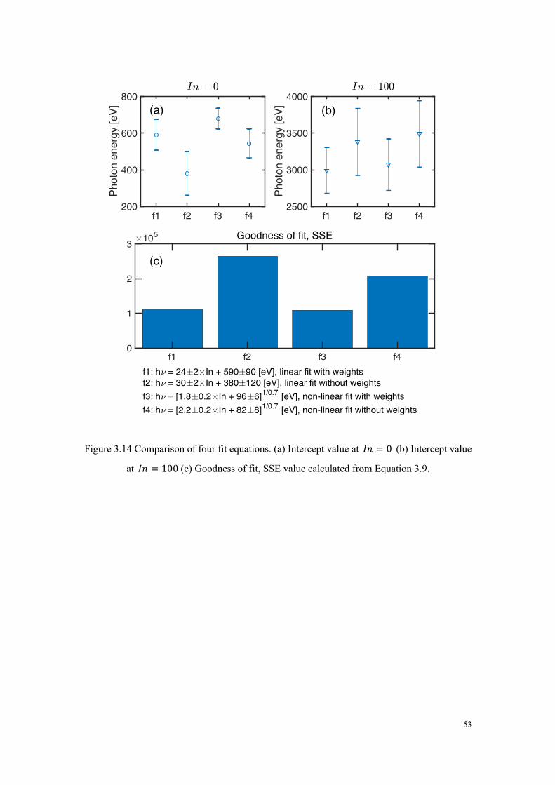
Figure 3.14 Comparison of four fit equations. (a) Intercept value at ôA = 0 (b) Intercept value

at ôA = 100(c) Goodness of fit, SSE value calculated from Equation 3.9.�

f1 f2 f3 f4200

400

600

800Ph

oton

ene

rgy

[eV]

f1 f2 f3 f42500

3000

3500

4000

Phot

on e

nerg

y [e

V]

Goodness of fit, SSE

f1 f2 f3 f40

1

2

3 105

(a) (b)

(c)

f1: h = 24 2 In + 590 90 [eV], linear fit with weightsf2: h = 30 2 In + 380 120 [eV], linear fit without weightsf3: h = [1.8 0.2 In + 96 6]1/0.7 [eV], non-linear fit with weightsf4: h = [2.2 0.2 In + 82 8]1/0.7 [eV], non-linear fit without weights

54

3.3. SXR spectra and Te calculation

Figure 3.15 shows the SXR spectra in the energy range 1.5–3.5 keV using energy

calibration function of Equation 3.6. The result has been corrected with quantum

efficiency of MCP detector and filter transmission. This energy range is free of the

characteristic radiation lines of metal and light impurities that are produced in other

tokamak devices [41].

The energy spectra produced by the left and right halves of the viewing area is

compared. The calculated bulk plasma temperature for each half is about 110–130 eV.

Unfortunately, electron temperature measurement for shot # 20268 and 20273 is not

available. Figure 3.16 shows the electron temperature measured by Thomson

Scattering (TS) in similar inboard limiter configuration of shot # 25477~25500. The

plasma current is about 10 kA, close to ô} in shot #20268 and 20273 (see Figure 3.2).

The heating power of 8.2 GHz ECW is 80 kW, close to that of shot #20268 and 20273.

The toroidal field of shot # 25477~25500 is st = 0.15T. The fundamental and second

harmonic resonance layer of the 8.2-GHz ECW is located at fuBv'l.GºΩæ = 0.33m and at

fuBvGl.GºΩæ = 0.66m, respectively. The electron temperature at 0.48 < f < 0.64r is

about CB ≈ 90~100 ± 30eV, while at 0.64r < f < 0.84r, CB ≈ 60~80 ±

15eV in shot # 25477~25500. This is a little bit lower than the calculation result in

Figure 3.15, probably due to only one cyclotron was used in shot # 25477~25500 (Only

RFPC).

It is seen in Figure 3.15 that the SXR spectra have a temperature component that is

much higher than the bulk temperature (260-400 eV). It indicates the presence of

higher-energy components in the RF current-driven plasma that might play an essential

role in non-inductive current driving. Because the second harmonic resonance layer lies

in left half (high field side), as shown in Figure 2.2 (b), the measured bulk electron

temperature in this half is higher than that in the right half (low field side).

55

Figure 3.15 SXR energy spectra corrected using the quantum efficiency of MCP

detector and filter transmission. The imaging area of the MCP assembly is divided

into a left half (f = 0.48– 0.66m) and a right half (f = 0.66– 0.84m). Core

plasma temperatures of 110 and 130 eV are derived from the fitting.

1.5 2 2.5 3 3.5Photon Energy (keV)

102

103

104

105

106

107

Inte

nsity

Left: R = 0.48~0.66 mRight: R = 0.66~0.84 m

140 10 eV

120 10 eV400 30 eV

260 20 eV

56

Figure 3.16 Electron temperature measured by Thomson Scattering (TS) in shot #

25477~25500. The plasma is in inboard limiter configuration, similar to shot # 20268 and

20273. The data is averaged over 20 shots at the same plasma conditions.

300 400 500 600 700 800 900 1000 1100 1200Major radius [mm]

-50

0

50

100

150

200

250

300Te

[eV]

TS measurement of shot #25477-25500, t = 3.5~3.6 s

57

3.4. Discussion

One of the assumptions for data deviation region in Figure 3.12 and Figure 3.13 is

that high energy SXR or HXR can penetrate the MCP and then directly reach the

phosphor screen. It was confirmed by the HX measurement that there are plenty of

energetic electron and HXR exist on QUEST plasma. According to the reference paper

(P.M. Shikhaliev, “Hard X-ray detection model for microchannel plate detectors”),

hard x-rays can penetrate into the MCP. As the phosphor is sensitive to SXR photons,

the phosphor screen can be illuminated by those photons that pass the MCP. These SXR

or HXR are not absorbed and amplified by the MCP, thus they cause additional photon

counting data in low ôA region.

ℜ =§•ú¶ßB + §}Évvdëø§•ú + §}Évvdëø

>§•ú¶ßB§•ú

= CßB (3.9)

The “passing photons” can cause a shift in ratio data. Most of passing photons

cause illumination at low ôA value compared with photons detected by MCP, because

the latter was amplified by secondary electrons. Thus, we expect the effect of “passing

photons” to be smaller at high ôA region.

Another possibility is that because of Compton scattering, the energy of scattered

photons became lower. We cannot confirm these assumptions using current data.

58

4. Imaging mode and plasma monitoring

Besides photon counting mode in which the system is used as photon counting

detector, the 2D-SXR system can be operated at imaging mode, when high spatial and

temporal resolution images of SXR emissivity were taken. It can be used as a plasma

monitor. Here the author presents two examples in imaging mode. The SXR image

intensity is calculated by summing the pixel intensities inside phosphor area (The green

area in Figure 2.9)

4.1. Slide-away electrons detection

Non-inductive current ramp-up has previously been obtained in QUEST through

the use of ECW [23, 43], and the generation and confinement of energetic electrons has

been shown to play an important role in driving plasma current [26]. Normally, the

presence of energetic electrons is indicated by the hard X-rays produced when the

electrons hit a wall. In this thesis, the author proposed an indirect detection method of

detecting impurity radiations caused by slide-away electrons.

Figure 4.1 shows the waveform of shot # 22069. At g = 1.2– 1.35s an 8.2 GHz

ECW of 50 kW was used to inductively drive a 10-kA plasma current during the period.

st increased from 0.13 T at 1.35 s to 0.26 T at 1.8 s. After inductively increasing to

about 50 kA, the plasma current began to decrease as the ECW power and Ohmic

heating were turned off. At g = 1.3a the ECW power was stopped, and the CS coil

current was decreased to drive and decelerate the plasma current. The CS coil current

began to decrease from g = 1.5a. As shown in Figure 4.1 (e–h), the drop in plasma

current created an enhancement of the loop voltage applied to the plasma, which

efficiently accelerated the electrons driving the plasma current.

Visible radiation measurement of spectral lines (Ha 656.461 nm, CIII 190.873 nm,

OII 372.709 nm) is available on QUEST. The data is shown in Figure 4.1 (c) and (g). It

is shown in Figure 4.1 (g) that carbon and oxygen impurities increase as a result of the

bombardment of slide-away electrons on the plasma-facing wall. The burst in SXR

signal is found to be consistent with CIII and OII signal, which suggested SXR

59

radiation came from the enhancement of impurities (see Equation 1.4), mostly Carbon

and Oxygen for QUEST plasma.

Figure 4.1 Waveforms of: (a) plasma current, ô}, and toroidal field coil current, ô¿¡; (b) Ohmic

heating by CS coil and ECW heating power; (c) hydrogen Balmer line radiation, Ha; and (d)

SXR intensity. (e–h) Zoomed waveforms of: (e) Ip; (f) loop voltage and Ha; (g), C, OII line

radiations; and (h) SXR intensity. I1–I3 denote the timing of SXR images in Figure 4.2.

0

20

40

60

Ip [k

A]

shot 22069

IpItf

0

5

10

CS [k

A]

Ohmic Heating8.2 GHz ECW (50kW)

0

1

2

3

H [a

.u.]

1.2 1.4 1.6 1.8Time [s]

0

2

4

6

SXR

[a.u

.]

35

40

45

50

Ip [k

A]

zoomed

-1

-0.5

0

vloop

[V]

0

0.5

1

1.5

H [a

.u.]

0

2

4

OII

[a.u

.]

0

2

4

CIII

[a.u

.]

1.45 1.5 1.55 1.6Time [s]

2

4

6

SXR

[a.u

.]

(a)

(b)

(c)

(d)

(e)

(f)

(g)

(h)I1

I3

I2

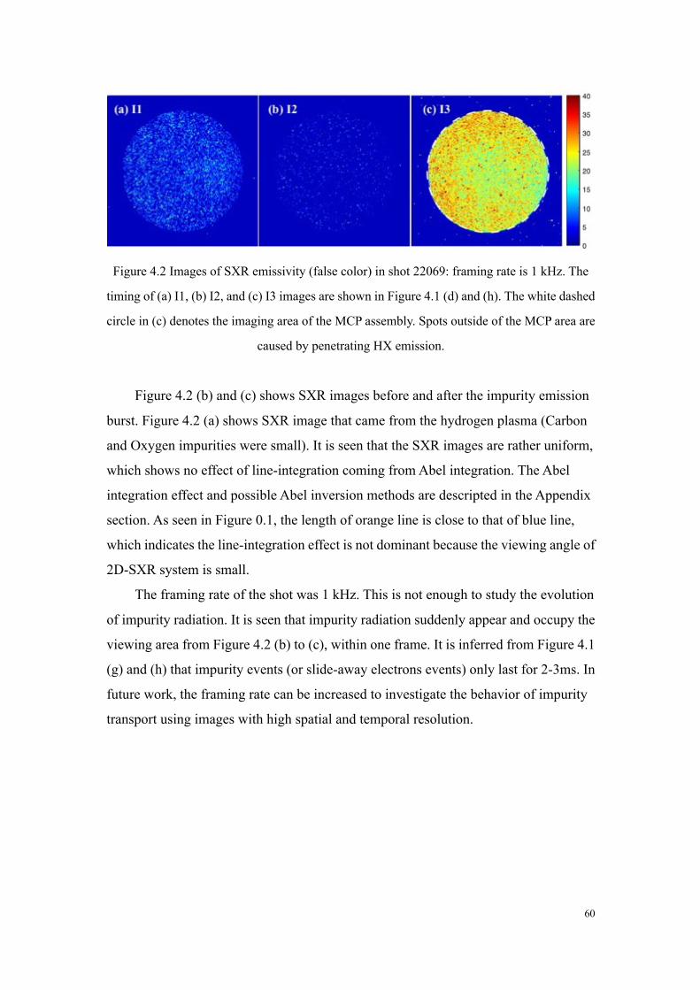
60

Figure 4.2 Images of SXR emissivity (false color) in shot 22069: framing rate is 1 kHz. The

timing of (a) I1, (b) I2, and (c) I3 images are shown in Figure 4.1 (d) and (h). The white dashed

circle in (c) denotes the imaging area of the MCP assembly. Spots outside of the MCP area are

caused by penetrating HX emission.

Figure 4.2 (b) and (c) shows SXR images before and after the impurity emission

burst. Figure 4.2 (a) shows SXR image that came from the hydrogen plasma (Carbon

and Oxygen impurities were small). It is seen that the SXR images are rather uniform,

which shows no effect of line-integration coming from Abel integration. The Abel

integration effect and possible Abel inversion methods are descripted in the Appendix

section. As seen in Figure 0.1, the length of orange line is close to that of blue line,

which indicates the line-integration effect is not dominant because the viewing angle of

2D-SXR system is small.

The framing rate of the shot was 1 kHz. This is not enough to study the evolution

of impurity radiation. It is seen that impurity radiation suddenly appear and occupy the

viewing area from Figure 4.2 (b) to (c), within one frame. It is inferred from Figure 4.1

(g) and (h) that impurity events (or slide-away electrons events) only last for 2-3ms. In

future work, the framing rate can be increased to investigate the behavior of impurity

transport using images with high spatial and temporal resolution.

61

4.2. Plasma oscillation

Another interesting observation of imaging mode is the plasma oscillation

phenomenon on QUEST. Onchi reported ~ 20-Hz oscillation in plasma current and heat

flux observed in inboard poloidal null configuration (IPN) in QUEST [44], as shown in

shot # 19418 in Figure 4.3. Plasma current remains above 20 kA and starts to oscillate

after the ô} ramp-up phase. Non-inductive current drive is realized by confining the

energetic trapped electrons produced 30 kW 8.2 GHz ECW. It is found the oscillations

are global in ô} and SOL parameters, which might be similar to relaxation oscillations

of the high-p} equilibrium. Similar relaxations have been observed on Hard X-ray

emission in TFR tokamak [45]. HXR measurement on QUEST also revealed on

oscillation of photon counts in IPN configuration [46], as shown in Figure 4.4. It is

considered that variation in HXs is because of the change in the confinement of the

energetic electrons depending on ô}.

62

Figure 4.3 Waveforms of typical discharge of IPN plasma with 20-Hz oscillation. The

parameters are as follows from the first panel: plasma current ô}, electron density

measured by the Langmuir probe at the top of the thermal probe head, estimated heat flux

¬BÑt and temperature at the probe head C¿Ä, Mach numbers at the far-SOL, and plasma

rotation (line of sight) velocity at the core. Cited from Onchi et. al [44]

63

Figure 4.4 Relaxation on Upper: plasma current and HXR; Lower: density of shot # 12006 in

IPN configuration on QUEST. Cited from [46]

Figure 4.5 Waveform of: (a) plasma current, ô}; (b) 8.2- and 28-GHz ECW heating (the

28-GHz power is much larger than 20kW, as shown in the figure); (c) Ha and (d) SXR intensity.

(e–h) Zoomed waveforms of: (e) Ip, (f) ion saturation current on upper divertor probes, (g) Ha

(h) SXR intensity of the three areas shown in Figure 4.6.

0

10

20

30

Ip [k

A]

0

20

40

60

ECW

8.2 GHz (50 kW)28 GHz

0

1

2

3

H [a

.u.]

2 2.5 3Time [s]

0

20

40

SXR

[a.u

.]

1416182022

Ip [k

A]

0

0.5

1

I sat,d

iv [A

]

1

1.5

2

H [a

.u.]

2.7 2.75 2.8Time [s]

0.40.60.8

1

SXR

[a.u

.] Left Mid Right

(a)

(c)

(d)

(e)

(b)

shot 22069 zoomed

(g)

(h)

(f)

64

Here, we report on the phenomenon of ~20-Hz low-frequency plasma oscillation

and its observation using the SXR imaging system. A typical waveform is shown for

shot # 22069 in Figure 4.5. The plasma oscillation occurs from 2.3– 2.9s under the

co-application of 8.2 and 28 GHz ECWs. The plasma is in limiter configuration, where

fdë = 0.2r. As shown in Figure 4.5 (a), the amplitude of ô}oscillation increases with

time. This low-frequency oscillation behavior is also seen in the Ha and SXR radiation,

which are in phase with each other. Although the oscillation is dominant in the plasma

core, it can also affect the plasma boundary, as indicated by the ion saturation current

signal on the upper divertor probes.

Figure 4.6 Images of SXR emissivity (false color) during one cycle of shot 22069. 15 out of 50

frames in one cycle are shown. The timing of frame 1 to frame 22 is 2.712 s to 2.733 s, with a

framing rate of 1 kHz. Three circular areas chosen to analyze spatial variation are shown in

frame 1; fuBvGGlºΩæ = 0.32m and fuBv'l.GºΩæ = 0.54m are indicated in frame 10 by cyan and

red dashed lines, respectively. The range of color map is [0, 12].

The shape and spatial evolution of a plasma oscillation can be monitored in the

imaging mode, as shown in Figure 4.6. The framing rate is 1 kHz. Only part of the

plasma oscillation cycle is shown here. It is seen that the oscillation activity is related to

spatial movement in the radial direction. The value of st is fixed at 0.26T during the

oscillation and the resonance layers of the 8.2- and 28-GHz ECWs are within the

observation window. The fundamental harmonic resonance layer of the 8.2-GHz ECW

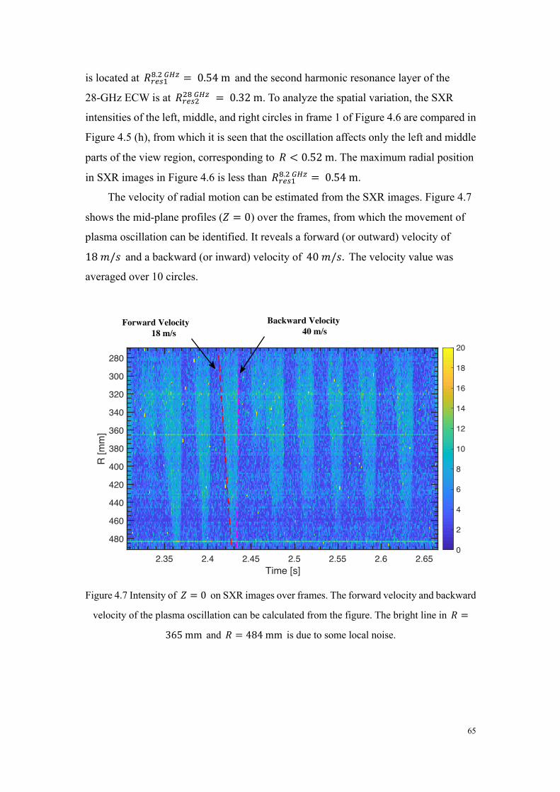
65

is located at fuBv'l.GºΩæ = 0.54m and the second harmonic resonance layer of the

28-GHz ECW is at fuBvGGlºΩæ = 0.32m. To analyze the spatial variation, the SXR

intensities of the left, middle, and right circles in frame 1 of Figure 4.6 are compared in

Figure 4.5 (h), from which it is seen that the oscillation affects only the left and middle

parts of the view region, corresponding to f < 0.52m. The maximum radial position

in SXR images in Figure 4.6 is less than fuBv'l.GºΩæ = 0.54m.

The velocity of radial motion can be estimated from the SXR images. Figure 4.7

shows the mid-plane profiles (V = 0) over the frames, from which the movement of

plasma oscillation can be identified. It reveals a forward (or outward) velocity of

18r/a and a backward (or inward) velocity of 40r/a. The velocity value was

averaged over 10 circles.

Figure 4.7 Intensity of V = 0 on SXR images over frames. The forward velocity and backward

velocity of the plasma oscillation can be calculated from the figure. The bright line in f =

365mm and f = 484mm is due to some local noise.

2.35 2.4 2.45 2.5 2.55 2.6 2.65Time [s]

280

300

320

340

360

380

400

420

440

460

480

R [m

m]

0

2

4

6

8

10

12

14

16

18

20

Backward Velocity 40 m/s

Forward Velocity 18 m/s

66

5. Summary and the future work

This thesis focused on the development and application of 2D-SXR imaging

system based on image intensifier with MCP detector on the QUEST tokamak. The

system was installed on a tangential port at mid-plane that watches the core area of

QUEST chamber. The field of view (FOV) can be changed in radial direction to match

the area of interest, which can cover the resonance layer of 8.2 GHz and 28 GHz

electron cyclotron wave (ECW) on QUEST.

Micro-channel plate (MCP) was used as the SXR detector and image intensifier,

which provides image gain of 10( that can be applied to low density plasma. As the

plasma density may be changed by a factor of 100 depending on different experimental

scenarios, and SXR emissivity may be changed by 10,000 times accordingly, the

flexible gain of image intensifier is important for operation in different plasma

parameters. The model of image gain was proposed, and tested by scanning the applied

voltage on MCP and phosphor.

Our system was compatible of both photon counting mode and imaging mode.

SXR spectra was obtained in photon counting mode with a framing rate of 100 kHz

provided by high speed camera. Energy calibration was performed using photon

counting data from two different filters, Al filter and “Al+Be”filter. Non-linear effect of

secondary emission was considered in the energy calibration, however, this effect

turned out to be smaller and the result is similar with linear fitting. Electron temperature

was derived from SXR spectra and energy calibration, which is in agreement with TS

data.

The imaging mode was applied to study fast variation of SXR emissivity in

plasma with fast and high spatial resolution images. The framing rate can be up to 1~10

kHz for the study of MHD instabilities. In this thesis, 1 kHz was used in the imaging

mode. Impurity radiation by slide-away electrons was observed by SXR images. Yet

the time resolution is not enough to catch up the details of spatial variation of impurity

radiation, which last for less than 1ms. An oscillation of ~20 Hz was observed in

plasma current, density, edge heat flux. Our system was applied to observe this plasma

oscillation phenomenon, which suggest a radial movement with forward velocity of 18

m/s and backward velocity of 40 m/s. This velocity is close to the current relaxation

67

time, which suggest the plasma oscillation was related to current relaxation.

While we use the system, we found some limitations of current system, which can

be improved in the future work. Possible improvements are listed as follows:

1) Reduce the cost of replacing MCPs

MCP is very fragile component and should be worked under high vacuum environment.

Gas can be easily absorbed in miniature electron multipliers inside MCP, which may

cause afterglow in the MCP, or even serious arcing problem and permanent damage to

the MCP. Left figure of Figure 5.1 shows SXR image with an inactive area in the

middle. This area, highlighted in the right figure, is caused by arcing inside the MCP.

Every image after that shows the same inactive part, denoting that the MCP has been

permanently damaged. We have to replace it.

Besides, there is a life time limit of the MCP. The electrical performance of MCP

becomes worse with time. Based on our experience, the life time is about two years.

Currently we use MCP assembly from PHOTONIS USA, INC. We have to replace the

whole assembly (including MCP, phosphor and vacuum flange), which is very

expensive. For the new system, we would like to use MCP from Hamamatsu Photonics,

INC. The MCP alone can be replaced, which can reduce the cost significantly.

2) Replace current “bare” MCP with a Cs-I coated or kBr-coated MCP

The detection efficiency of “bare” MCP to SXR is rather low (about 5~15%). We would

like to replace with alkali halide coated MCP for higher detection efficiency (up to the

50% reported for CsI photocathodes [47]).

3) Replace the shutter and Al filter with a vacuum Be window

One of the largest limitations in 2D-SXR imaging system is that it only watches the

center of QUEST chamber. This is due to a gate valve and openable shutter were

installed (see Figure 2.3) in front of pinhole plate and MCP detector, so that the distance

of MCP detector to the vacuum window is large (about 65 cm). Therefore, we would

like to replace the shutter and Al filter with a vacuum Be window that can withstand the

atmospheric pressure. Be window of 40 μm has been used in SXR camera in LHD [48].

It can simplify the design of the system and allow the MCP to be placed much closer to

the QUEST plasma without incurring arcing from QUEST gas injection. These

improvements will extend the viewing area into the edge region, which will enable the

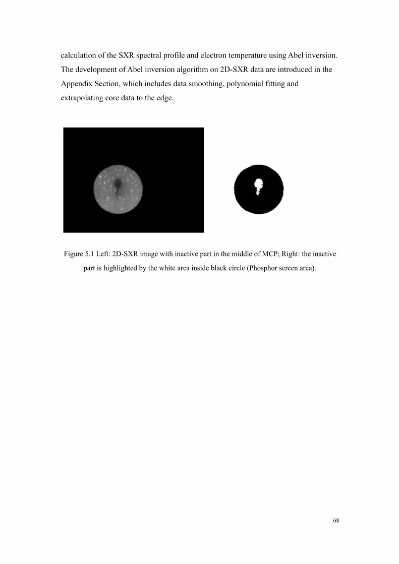
68

calculation of the SXR spectral profile and electron temperature using Abel inversion.

The development of Abel inversion algorithm on 2D-SXR data are introduced in the

Appendix Section, which includes data smoothing, polynomial fitting and

extrapolating core data to the edge.

Figure 5.1 Left: 2D-SXR image with inactive part in the middle of MCP; Right: the inactive

part is highlighted by the white area inside black circle (Phosphor screen area).

69

Appendix: Abel inversion on 2D-SXR profile

Tomography reconstruction has been widely used in 1D SXR arrays to reconstruct

local plasma emissivity [5, 10]. A special case of this reconstruction problem is the

Abel transformation, which has to be used in the study of radially symmetrical objects,

side-on observation of a plasma column in Tokamaks. As shown in Figure 0.1 (a), if an

unknown function ≥(√) can be only measured by integrating it along straight-line

paths, thus producing the projection ℎ(ƒ). The relation between these two functions is

given by the forward Abel transformation [49]

ℎ(ƒ) = 2≈≥(√)√

∆√G − ƒGO√

«

»

(0.1)

The reconstruction of the unknown function ≥(√) from the measured data ℎ(ƒ) can

be done analytically by means of the inverse Abel transformation [49]

≥(√) = −1…≈

Oℎ(ƒ)Oƒ

Oƒ∆ƒG − √G

«

»

(0.2)

Figure 0.1 Illustration figure of Abel inversion in (a) plane projection (b) pinhole projection.

The location of MCP plate and pinhole are plotted.

This is the case of plane projection. It has been fully discussed and there are many

algorithms to solve this problem, as discussed in Section 5.2. However, the Abel

inversion problem for 2D-SXR system on QUEST is much more complicated, due to

70

the following reasons:

1) The 2D-SXR images is formed through a pinhole.

It is a pinhole projection problem in Figure 0.1 (b). It can be solved by transforming the

pinhole projection into plane projection. For instance, the line-integration signal of the

orange line equals to that of the orange dash line, because of cylindrical symmetry and

both lines have the radial of tangency √¿.

Consider 1D problem. The SXR power emitted by a local volume element and later

filtered by a filter and absorbed by the MCP detector is given by [5]

À(√) = ≈OP(√)OℎQ

EÃ

EÕ∙ CWdútBu ∙ C~�Ä ∙ O(ℎQ) (0.3)

where the plasma continuum radiation òÄ(u)òîŒ

is given by Equation 1.4, nœ and n– is

the lower and upper energy limit of detected photons.

The tangential, line-integrated SXR brightness at the plasma midplane can be

calculated using forward Abel transformation

ℬ(√¿) = 2 ≈ À(√)√

∆√G − √¿GO√

«“”‘

u’

(0.4)

Where fÇÉÑ = 1.37m is the radius of QUEST vacuum chamber. Suppose the

intensity of SXR image in y direction is ô(ƒë), which comes from the line-integration

signal of orange line in Figure 0.1 (b). The mapping function between ƒë and √¿ is

found using the geometry relationships

± = tanS' ©ƒë − ƒxπ}v − πx

™ (0.5)

f¿ = ƒx − πx ∙ tan ± =π}vƒx − πxƒëπ}v − πx

(0.6)

√¿ = ◊(ƒë) = f¿ ∙ cos ± (0.7)

Where ± is the angle between the orange line and blue line (parallel to x axis), f¿ is

the intercept of orange line with y axis, √¿ is the radial of tangency of orange line, (πx,

ƒx) is the pinhole position, π}v is the position of phosphor screen. Therefore, local

SXR emissivity À(√, g) can be calculated using inverse Abel transformation

(Equation 0.2) and mapping function (Equation 0.7) from the input data ô(ƒë, g).

2) It is a 2D image reconstruction.

71

Real images are two-dimensional function of ô(ƒë, ÿë), where z direction is the vertical

direction. It is difficult to calculate Abel inversion of ô(ƒë, ÿë), ÿë ≠ 0, because the

lines of sight are oblique. Up-down symmetry should be assumed in 2D images.

However, up-down symmetry is not guaranteed in real plasma. In this thesis, the author

only reconstructed the 1D profile on mid-plane (ÿë = 0), where the toroidal symmetry

is satisfied. The full reconstruction of 2D images remain as a future work.

3) 2D-SXR imaging system only have limited spatial coverage in QUEST chamber.

For instance, the area between blue line and orange line in Figure 0.1 (b) denotes the

coverage of 2D-SXR imaging system. The spatial coverage is limited by the chamber

port size, distance of pinhole plate and MCP assembly to the port. The edge signals are

required to fully reconstruct local SXR emission profile from Equation 0.2. This is

solved by assuming the edge signals according to extrapolation of the known center

signals.

There are many different numerical approaches to solve the integral in Equation

0.2, see e.g. [49-52]. These methods have different performance in terms of speed,

accuracy, resistance to noise. The realization of these methods is available in an

open-sourced python library called PyAbel (https://pyabel.readthedocs.io/en/latest/).

The author used Python and openCV for Abel inversion and digital image processing in

this chapter.

The methods used in this thesis consist of

1) Direct method

Direct method is direct integration of the Abel transform integral (Equation 0.3

and 0.4). It makes no assumptions about the data (apart from cylindrical symmetry), but

it typically requires fine sampling to converge.

2) BASEX method

The idea of BASEX method is to have basis functions ≥c⁄ in the space of distributions

≥ [51][51][51]. The choice of base functions can be made arbitrarily but it is useful if

they satisfy following properties:

l Every function should be easily analytically integrable to perform the

Abel-transformation

72

l Intensity-distributions obtained by this transformation shall permit imaging of

sufficiently small structures

l The projections shall be sufficiently smooth on even smaller distances

3) Hansenlaw method

This method is developed by Hansen et al [52]. It has the advantage that it can be used

on arbitrary length data, and the data do not have to have constant spacing along the

x-axis.

4) Onion peeling� Two-point and Three-point method

These methods are introduced by Cameron Dasch [50]. In the onion-peeling method

the projection is approximated by rings of constant property between √¤ − ∆√ 2⁄ and

√¤ + ∆√ 2⁄ for each data point √¤, where ∆√ is the spatial resolution.

In order to test the accuracy of these methods, analytical expressions of Forward

and Inversion Abel transformation profiles are necessary. Here we adopted the gaussian

profile and other profiles from [53-57].

73

Table 0.1 Mathematical descriptions of the test profiles used in this work

Theoretical radial !(#) and lateral ℎ(&)profile Refs.

1 !(#) = exp ,

−#.

/.0 , 0 ≤ # ≤ 1

ℎ(&) = /√6exp ,−&.

/.0 , 0 ≤ & ≤ 1

2 !(#) = 7

1 − 2#., 0 ≤ # ≤ 0.52(1 − #)., 0.5 ≤ # ≤ 1

ℎ(&) =

⎩⎨

⎧43@A(1 + 2&C) −

[email protected]

(1 + 8&.) − 4&. ln1 + @A

0.5 + @D.E, 0 ≤ & ≤ 0.5

43@A(1 + 2&C) − 4&. ln

1 + @A&

, 0.5 ≤ & ≤ 1

[53,

54]

3 !(#) = 1 − 3#. + 2#C, 0 ≤ # ≤ 1

ℎ(&) = @A I1 −52&.J +

32&K ln

1 + @A&

, 0 ≤ & ≤ 1

[54]

74

4 !(#) = L

0.75 + 12#. − 32#C, 0 ≤ # ≤ 0.251627(1 + 6# − 15#. + 8#C), 0.25 ≤ # ≤ 1

ℎ(&) =

⎩⎨

⎧1108

(128@A + @D..E) +227&.([email protected] − 112@A) +

89&. P4(1 + &.) ln

1 + @A&

− (4 + 31&.) ln0.25 + @D..E

&Q , 0 ≤ & ≤ 0.25

3227I@A − 7@A& + 3&.(1 + &.) ln

1 + @A&

J , 0.25 ≤ & ≤ 1

[54]

5 !(#) = (1 − #.)

RC. exp P1.1. I1 −

11 − #.

JQ , 0 ≤ # ≤ 1

ℎ(&) =√61.1@A

exp P1.1. I1 −1

1 − &.JQ , 0 ≤ & ≤ 1

[55]

6 !(#) =

12(1 + 10#. − 23#K + 12#S), 0 ≤ # ≤ 1

ℎ(&) =8105

@A(19 + 34&. − 125&K + 72&S), 0 ≤ & ≤ 1

[55]

7 !(#) = [−47.7(1 − #.)U + 43.5(1 − #.)S + 5.5(1 − #.)E − 0.9(1 − #.)K]/3, 0 ≤ # ≤ 1

ℎ(&) = [−30.361(1 − &.)U.E + 29.667(1 − &.)S.E + 4.063(1 − &.)E.E − 0.9731(1 − &.)K.E]/3, 0 ≤ & ≤ 1

[56]

In the table, @X is defined as Y(Z. − &2). Test function 1 is the gaussian distribution, and / is its variance.

75

Figure 0.2 Theoretical (a) radial emissivity !(#) and (b) lateral emission ℎ(&) of the seven

test profiles used in this study. The radial and lateral position is normalized to 1. The

mathematical expression of test profiles is shown in Table 0.1. For profile-1, ' = 0.5.

76

Figure 0.2 shows the (a) radial emissivity!(#) and (b) lateral emissionℎ(&) of

the seven test profiles. The radial emissivity !(#) is the Abel inversion of lateral

emission ℎ(&). The outmost lateral and radial position of test functions have been

normalized to 1. And the edge emissivity !(# = 1), ℎ(& = 1) should be zero or very

small. Profile 1-3 peak at the center # = 0 while profile 4-7 peak at elsewhere.

The above mentioned six methods are tested using the gaussian distribution. The

result is shown in Figure 0.3. The lateral emission profile ℎ(&) of profile-1 is used as

the input signal. The Abel inverted profile using six methods is shown in Figure 0.3 (a).

It is seen that all six methods can reconstruct ideal gaussian distribution (noise-free)

pretty well, except at the edge and center. In the thesis, the relative residue ∆012, is

defined as the error between Abel-inverted profile and theoretical profile [57]

∆012(#3) = !4524(#3) − !7819(#3)

∑ !7819(#3);<=3>?

(0.8)

Where !4524(#) is the calculated profile using the Abel inversion method, and !7819(#)

is the theoretical profile. A is the number of data in the profile. Total relative residue is

used for comparison of the reconstruction error between different profiles

Τ = C|∆012(#3)|

;<=

3>?

(0.9)

Figure 0.3 (b) shows the relative residue profile in percentage. It is seen that the

error is less than 0.02% in 0.1 < # < 0.9 for all methods. The BASEX method, onion

method, two-point and three-point method have large error at the edge # > 0.9. (The

edge goes up in Figure 0.3 (a)). For the center signal# < 0.1, the BASEX method,

onion method and three points method have small error. Figure 0.3 (c) shows the total

relative residue of all data and data at the center (0.1 < # < 0.9). Basically, the BASEX

method and three-point method give the best reconstruction. This is only applicable to

the noise-free signal.

77

Figure 0.3 Abel inversion of profile-1 ℎ(&) using six methods. Number of data is 101. (a) The

Abel inversion result !4524(#). Each curve is offset from the nearest by 0.1 unit for clarity. (b)

The relative residue profile ∆#HI in percentage, calculated from Equation 0.8. (c) Total relative

residue of all data and data except the edge (# < 0.9).

78

It is known that Abel-inverted radial profile exhibits the greatest error in the center

of the source (i.e., when # → 0), since measurement error and noise propagate from the

edge to the center of the source (see Equation 0.2). Moreover, the Abel inversion is very

sensitive to noise in the lateral profile because the derivative of ℎ(&) (i.e. Kℎ(&) K&⁄ )

is used in Equation 0.2. Figure 0.4 (a) shows the example of profile-4 added with no

noise, and with 0.1%, 0.3% and 1% gaussian noise. Here the 1% gaussian noise means

~68% of the noise magnitude is within 1% of the signal strength. Figure 0.4 (b) shows

the Abel-inverted profile calculated by Hansenlaw method without any data smoothing

or noise filtering. It is evident that even a noise level of 0.3% in the lateral emission

profile could cause large error in the Abel-inverted profile. For lateral emission profile

with a noise level of 1%, it is difficult to identify the peak location in its Abel-inverted

profile.

Figure 0.5 compares the performance of all six methods using profile-2 added

with 0.3% gaussian noise. Each curve in Figure 0.5 (a) is offset from the nearest by 0.1

unit for clarity. The Abel-inverted profiles are similar by different methods, but the

noise amplitude in each profile is different. Figure 0.5 (b) shows the error of Abel

inversion (from Equation 0.8). The error is larger at the center, because the noise

propagates from the edge to the center. It is seen in Figure 0.5 (c) that direct method,

Hansenlaw method and three-point method have the highest performance with noisy

profiles. This is also true for other profiles (The result is not shown here).

The random noise in the 2D-SXR images can be reduced by averaging over

images in which the plasma parameters are constant, and the image profiles are also

identical.

Besides, digital smoothing and image denoising methods can be applied to further

reduce the effect of noise. One of the typical methods is to apply a low pass filter to

filter out the high frequency noise in the image. It can be accomplished by doing a

convolution between a blur kernel and the image. Linear filter such as moving average

filter or gaussian filter are usually used. Non-linear filter such as median filter is not

preferable, even if it can reduce salt-and-pepper noise effectively.

79

Figure 0.4 (a) Lateral emission profile with 0%, 0.1%, 0.3% and 1%

added noise in profile-4. (b) Abel-inverted radial emission profile

from the lateral emission profiles in (a), with 0%, 0.1%, 0.3% and 1%

added noise. Hansenlaw method is used for Abel inversion. Each

curve is offset from the nearest by 0.1 unit for clarity in (a) and (b).

80

Figure 0.5 Comparison of Abel inversion to profile-2 with 0.3% gaussian noise. (a) The Abel

inversion result !4524(#). Each curve is offset from the nearest by 0.1 unit for clarity. (b) The

relative residue profile ∆#HI in percentage, calculated from Equation 0.8. (c) Total relative

residue of all data and data except the edge (# < 0.9).

The 1D kernel function of moving average filter and gaussian filter is given by

MN15O(P) =1

QRPSH(0.10)

MT5UVV35O(P) = W × exp[−(P − (QRPSH − 1) 2⁄ )^ (2')^⁄ ] (0.11)

Where QRPSH is the blurring kernel size, which should be positive and odd. P =

0,1, . . , QRPSH − 1. W is the scale factor chosen so that ∑ MT5UVV35O(P) =3 1. It is also

required that ∑ MN15O(P) =3 1, so that the blurring kernel wouldn’t change mean value

81

of the signal. The sigma ' in gaussian filter can be any positive value. Here we use its

default value in OpenCV which is computed from QRPSH

' = 0.3 × a√QRSPH − 1 − 1c + 0.8 (0.12)

Note image padding is necessary in calculating the convolution between an image with

a kernel. The author padded the image with replicates of the image border, in order not

to affect the mean value of pixels in the border.

Figure 0.6 shows the result of image smoothing using moving average filter and

gaussian filter. Profile-7 with 3% gaussian noise is used as test function. The kernel size

from 3 to 19 is scanned for optimization. The Hansenlaw method is used for Abel

inversion of smoothed profiles. The smoothed profiles and Abel-inverted profiles are

shown in (a,c) and (b,d), respectively. The accuracy (total residue error) is shown in

Figure 0.6 (e). Generally speaking, moving average filter has better performance in

reducing the error than gaussian filter. For gaussian filter, the accuracy is higher with

larger kernel size. However, larger kernel size causes longer computing time. For

moving average filter, there is an optimum kernel size of 11, which is about one tenth of

the data number (A = 101). Note the smoothing kernels can be applied again to the

Abel-inverted profiles to reduce the noise further.

Another method discussed in this paper is smoothing by polynomial fit [56]. It

means to apply a polynomial function to fit the data

e3 = f? + f=g3 + f^g3^ + ⋯+ fOg3

O, (P = 1,2, … , j) (0.13)

Where j is the highest order of polynomial function, and the coefficient f is

determined by the least squares method. Figure 0.7 shows the result of polynomial

smoothing. Profile-7 with 3% gaussian noise is used as test function. The Hansenlaw

method is used for Abel inversion of the smoothed profiles. It is seen that 3-order

polynomial function is not enough to fit the test function, thus producing very large

error. The total relative error is almost constant for j ≥ 5. Actually, high order

polynomial function may cause overfitting in the center as seen in Figure 0.7 (b). The

optimum result is about j = 4~6. This is also true for other profiles. The total relative

error of j = 5 in Figure 0.7 (c) is about 0.029, less than the minimum total relative

error in moving average filter and gaussian filter (about 0.04). It indicates the

performance of polynomial smoothing is better than image blurring. The reason maybe

polynomial fitting is global (all data are used for fitting in Equation 0.13).

82

Figure 0.6 Comparison of two smoothing kernels and kernel size. Profile-7 with 3% gaussian

noise is used as test function. Each curve is offset from the nearest by 0.1 unit for clarity. (a)

Smoothing using moving average filter; (b) Abel-inversion of smoothed profiles in (a); (c)

Smoothing using gaussian filter; (b) Abel-inversion of smoothed profiles in (c); (e) Total

relative residue of two kernels and kernel size from 3 to 19.

83

Figure 0.7 Comparison of polynomial smoothing. Profile-6 with 3% gaussian noise is used as

test function. Each curve is offset from the nearest by 0.1 unit for clarity. (a) Smoothing using

polynomial fit (b) Abel-inversion of smoothed profiles in (a); (c) Total relative residue of all

data and data in the 0.1 < # < 0.9.

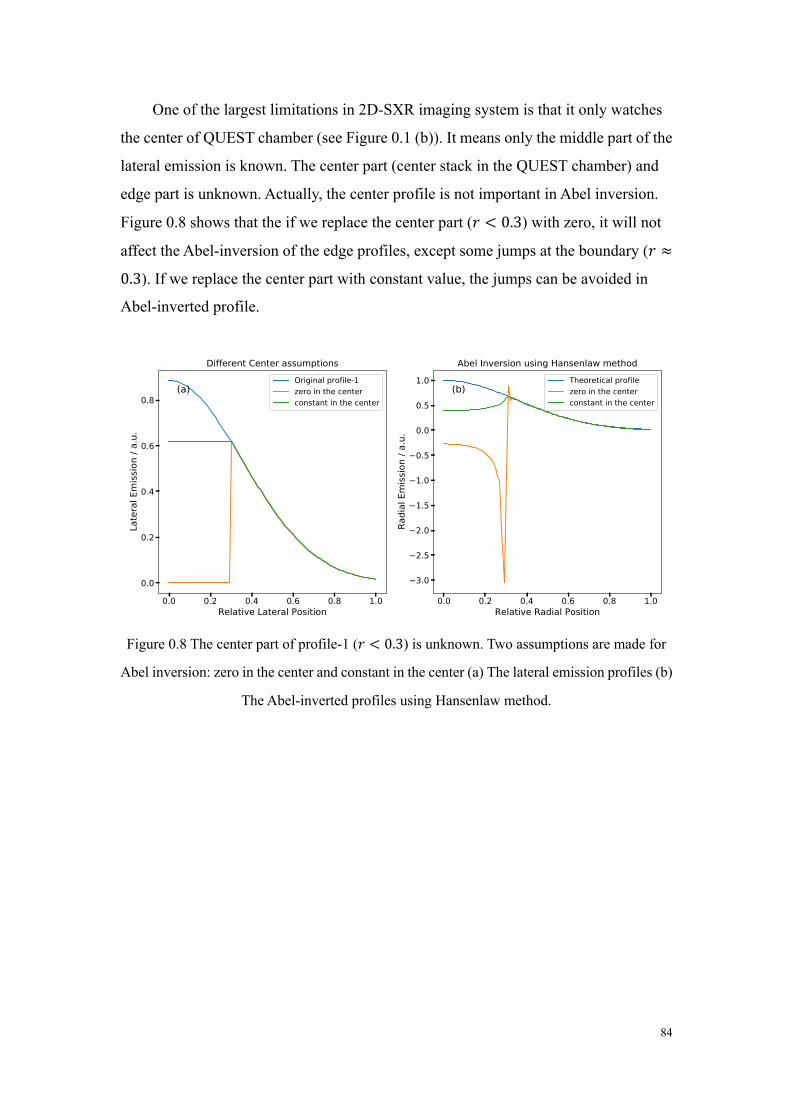
84

One of the largest limitations in 2D-SXR imaging system is that it only watches

the center of QUEST chamber (see Figure 0.1 (b)). It means only the middle part of the

lateral emission is known. The center part (center stack in the QUEST chamber) and

edge part is unknown. Actually, the center profile is not important in Abel inversion.

Figure 0.8 shows that the if we replace the center part (# < 0.3) with zero, it will not

affect the Abel-inversion of the edge profiles, except some jumps at the boundary (# ≈

0.3). If we replace the center part with constant value, the jumps can be avoided in

Abel-inverted profile.

Figure 0.8 The center part of profile-1 (# < 0.3) is unknown. Two assumptions are made for

Abel inversion: zero in the center and constant in the center (a) The lateral emission profiles (b)

The Abel-inverted profiles using Hansenlaw method.

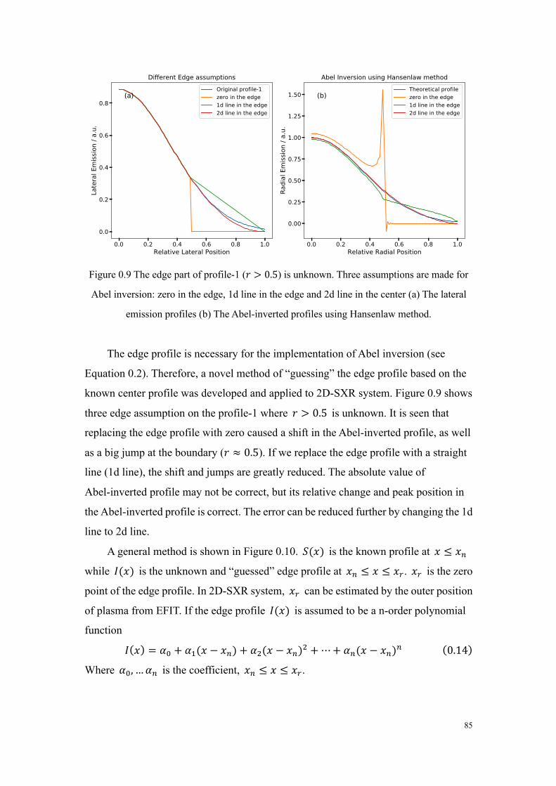
85

Figure 0.9 The edge part of profile-1 (# > 0.5) is unknown. Three assumptions are made for

Abel inversion: zero in the edge, 1d line in the edge and 2d line in the center (a) The lateral

emission profiles (b) The Abel-inverted profiles using Hansenlaw method.

The edge profile is necessary for the implementation of Abel inversion (see

Equation 0.2). Therefore, a novel method of “guessing” the edge profile based on the

known center profile was developed and applied to 2D-SXR system. Figure 0.9 shows

three edge assumption on the profile-1 where # > 0.5 is unknown. It is seen that

replacing the edge profile with zero caused a shift in the Abel-inverted profile, as well

as a big jump at the boundary (# ≈ 0.5). If we replace the edge profile with a straight

line (1d line), the shift and jumps are greatly reduced. The absolute value of

Abel-inverted profile may not be correct, but its relative change and peak position in

the Abel-inverted profile is correct. The error can be reduced further by changing the 1d

line to 2d line.

A general method is shown in Figure 0.10. p(g) is the known profile at g ≤ gO

while r(g) is the unknown and “guessed” edge profile at gO ≤ g ≤ g0. g0 is the zero

point of the edge profile. In 2D-SXR system, g0 can be estimated by the outer position

of plasma from EFIT. If the edge profile r(g) is assumed to be a n-order polynomial

function

r(g) = W? + W=(g − gO) + W^(g − gO)^ + ⋯+ WO(g − gO)

O (0.14)

Where W?, …WO is the coefficient, gO ≤ g ≤ g0.

86

Figure 0.10 Illustration of polynomial fitting and extrapolation. p(g) is the known

profile at g ≤ gO, r(g) is the “guessed” edge profile at gO ≤ g ≤ g0, where g0

is the zero point of r(g). The derivatives of r(g) and S(g) is the same at gO.

The signal p(g) can be fitted by a (n-1) order polynomial function

p(g) = f? + f=(g − gO) + f^(g − gO)^ + ⋯+ fO<=(g − gO)

O<= (0.15)

Where f?, …fO<= is the coefficient of polynomial fitting, 0 ≤ g ≤ gO.

The unknown coefficient in Equation 0.15 can be calculated using the derivatives

of p(gO) and end point g0by the following equations

r(gO) = p(gO)

rs(gO) = ps(gO)(0.16)

⋮rO<=(gO) = pO<=(gO)

r(g0) = 0

In this case the edge profile r(g) is perfectly connected with center profile p(g) and

confined by the end point. Equation 0.16 yields W? = f?

W= = f=(0.17)

⋮WO<= = fO<=

WO = −W? + W=∆g +⋯+ WO<=∆g

O<=

∆gO,∆g = g0 − gO

Next step we would like to test this method with the test functions of Profiles 1-7.

The left half of Profiles 1-7 (0 ≤ g ≤ 0.5) are used as the input p(g), and edge profile

r(g) (0.5 ≤ g ≤ 1) is calculated according to this algorithm. Then the whole profile is

reconstructed using Abel inversion and compared with the theoretical profile. The

BASEX method is used for Abel inversion. The results of Profile-1 to Profile -7 are

shown in Figure 0.11 to Figure 0.13, respectively. Generally speaking, the total relative

residue becomes smaller with larger n, where n is the highest order of r(g). The total

87

relative residue for left half data (this is what we care about) is in the order of

1 × 10<v~1 × 10<w, when n is about 4~5. However, for some cases large n causes

overfit, such as j ≥ 6 in Profile-2 (Figure 0.12). In fact, the edge profile r(g) should

be a monotonically decreasing function, which requires

rs(g) < 0, (gO ≤ g ≤ g0) (0.18)

The overfit curve is easy to identify, thus can be avoided manually. If there is an

overfit, it means smaller n should be chosen. Another exception is that r(g) may be

less than 0, such as j ≥ 6 in Profile-5 (Figure 0.13). This can be avoided by changing

the zero point g0 to other zero point r(g3) = 0, g3 < g0. For future work, the author

would like to include Equation 0.18 in the algorithm.

88

Figure 0.11 Polynomial fit and extrapolation. Left half of profile-1 (0 < # < 0.5) is used as the

input. (a) Edge profile (0.5 < # < 1) is guessed by n-d lines, n is the highest polynomial order

of edge profile (b) Abel-inversion of profiles in (a); (c) Total relative residue of all data and data

in the left half 0 < # < 0.5.

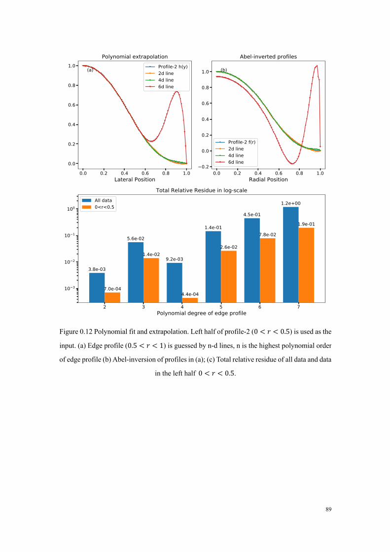
89





90





91

List of publications

Papers [1] Canbin Huang, K. Hanada, …, et al, “Fast Tangentially Viewed Soft X-Ray

Imaging System Based on Image Intensifier with Microchannel Plate Detector on

QUEST”, Plasma and Fusion Research 14, 1402128 (2019).

[2] K. Kuroda, …, C. Huang, et al, “Initial results from solenoid-free plasma start-up

using Transient CHI on QUEST”, Plasma Phys. Control. Fusion 60 (2018) 115001

[3] K. Hanada, …, C. Huang, et al, “Estimation of fuel particle balance in steady

state operation with hydrogen barrier model”, Nuclear Materials and Energy 19 (2019)

544–549

Conferences [1] C. Huang, K. Hanada et al, “Result of transient Coaxial Helicity Injection

experiments on QUEST”, Poster, the 27th International Toki Conference on Plasma and

Fusion Research, National Institute for Fusion Science, Toki, Gifu, Japan, 2018.11.19-22

[2] C. Huang, K. Hanada et al, “Initial results of Transient Coaxial helicity injection

experiments on QUEST”, Poster, the 12nd Fusion Energy Joint Conference, Saga,

Japan, 2018.6.28

[3] C. Huang, K. Hanada et al, “Observation of ELM mitigation by counter current

direction NBI on EAST”, Oral, the 72nd Annual Meeting of the Japanese Physical

Society, Osaka, Japan, 2017.3.17-20

[4] C. Huang, K. Hanada et al, “High spatial and temporal resolution measurement of

2D-SXR on QUEST”, Oral, the 5th A3 Foresight Workshop on ST, Kunming, Yunnan,

China, 2017.2.15-17

[5] C. Huang, K. Hanada et al, “Study of steady-state operation and ELM control in

tokamak”, Oral, the 18th Cross Straits Symposium on Energy and Environmental Science

and Technology (CSS-EEST18), Shanghai, China, 2016.12.4-6

92

References

1. IEA, I., Key World Energy Statistics, 2013. 2013, International Energy Agency

publication.

2. Wesson, J. and A.K. Sen, Tokamaks. Physics Today, 1989. 42: p. 78.

3. Horvath, A. and E. Rachlew, Nuclear power in the 21st century: Challenges

and possibilities. Ambio, 2016. 45(1): p. 38-49.

4. Ushigusa, K. Steady state operation research in JT-60U. in Fusion energy 1996.

V. 1. Proceedings of the 16. international conference. 1997.

5. Delgado-Aparicio, L.F., et al., Fast electron temperature measurements using a

"multicolor" optical soft x-ray array. Journal of Applied Physics, 2007. 102(7).

6. Rice, J.E., K. Molvig, and H.I. Helava, Continuum x-ray emission from the

Alcator A tokamak. Physical Review A, 1982. 25(3): p. 1645.

7. Sun, Z., et al., Real time wall conditioning with lithium powder injection in long

pulse H-mode plasmas in EAST with tungsten divertor. Nuclear Materials and

Energy, 2019. 19: p. 124-130.

8. Patel, A., et al., Z eff profile measurements from bremsstrahlung imaging in the

MAST spherical tokamak. Review of scientific instruments, 2004. 75(11): p.

4944-4950.

9. Sharma, S., et al., Analysis of PWI footprint traces and material damage on the

first walls of the spherical tokamak QUEST. Fusion Engineering and Design,

2012. 87(1): p. 77-86.

10. Hanada, K., et al., COMPUTER-TOMOGRAPHY OF M=1 MODE DURING

SAWTOOTH OSCILLATION WITH 3 SOFT-X-RAY DETECTOR ARRAYS ON

THE WT-3 TOKAMAK. Plasma Physics and Controlled Fusion, 1990. 32(14): p.

1289-1299.

11. Tritz, K., et al., Compact "diode-based" multi-energy soft x-ray diagnostic for

NSTX. Review of Scientific Instruments, 2012. 83(10).

12. Delgado-Aparicio, L., et al., High-efficiency fast scintillators for" optical" soft

x-ray arrays for laboratory plasma diagnostics. Applied optics, 2007. 46(24): p.

6069-6075.

13. Liang, Y., et al., Energy and spatial resolved measurement of soft x-ray emission

93

with photon counting x-ray charge coupled device camera in compact helical

system. Review of Scientific Instruments, 2000. 71(10): p. 3711-3717.

14. Tritz, K., et al., Tangential soft x-ray imaging for shape and current profile

measurements. Review of scientific instruments, 2003. 74(3): p. 2161-2164.

15. Zhou, F., et al., Development of a high-speed vacuum ultraviolet (VUV)

imaging system for the Experimental Advanced Superconducting Tokamak.

Review of Scientific Instruments, 2017. 88(7).

16. Shi, Y., et al., Soft x-ray pulse height analyzer in the HT-7 tokamak. Review of

scientific instruments, 2004. 75(11): p. 4930-4933.

17. Jin, W., et al., Development of a soft X-ray pulse height analyzer on the J-TEXT

tokamak. Nuclear Instruments and Methods in Physics Research Section A:

Accelerators, Spectrometers, Detectors and Associated Equipment, 2012. 674:

p. 15-19.

18. Hill, K., et al., Tokamak Fusion Test Reactor prototype x‐ray pulse‐height

analyzer diagnostic. Review of Scientific Instruments, 1985. 56(5): p. 840-842.

19. Tashima, S., et al., Hard X-ray measurement during the current startup phase in

QUEST. Journal of Plasma and Fusion Research Series, 2010. 9: p. 316-321.

20. Ishiguro, M., et al., Non-inductive current start-up assisted by energetic

electrons in Q-shu University experiment with steady-state spherical tokamak.

Physics of Plasmas, 2012. 19(6): p. 11.

21. Hanada, K., et al., Steady-state operation scenario and the first experimental

result on QUEST. Plasma and Fusion Research, 2010. 5: p. S1007-S1007.

22. Hanada, K., et al., Estimation of fuel particle balance in steady state operation

with hydrogen barrier model. Nuclear Materials and Energy, 2019. 19: p.

544-549.

23. Idei, H., et al., Fully non-inductive second harmonic electron cyclotron plasma

ramp-up in the QUEST spherical tokamak. Nuclear Fusion, 2017. 57(12).

24. Yamada, T., 2D-SXR imaging system, in Interdisciplinary Graduate School of

Engineering Sciences. 2014, Kyushu University.

25. Fujiyoshi, H., 2D-SXR imaging system on QUEST, in Interdisciplinary

Graduate School of Engineering Sciences. 2016, Kyushu University.

26. Tashima, S., et al., Role of energetic electrons during current ramp-up and

production of high poloidal beta plasma in non-inductive current drive on

94

QUEST. Nuclear Fusion, 2014. 54(2): p. 11.

27. Wiza, J.L., MICROCHANNEL PLATE DETECTORS. Nuclear Instruments &

Methods, 1979. 162(1-3): p. 587-601.

28. Han, L., et al., The effect of gain variation in micro-channel plates on

gamma-ray energy resolution, in Medical Applications of Radiation Detectors

Iii, H.B. Barber and H. Roehrig, Editors. 2013.

29. Hirata, M., et al., X‐ray detection characteristics of microchannel plates using

synchrotron radiation in the energy range from 0.06 to 0.6 keV. Review of

scientific instruments, 1990. 61(10): p. 2566-2570.

30. Hill, G., Secondary Electron Emission and Compositional Studies on Channel

Plate Glass Surfaces. Advances in Electronics and Electron physics, 1976: p.

153.

31. Scholtz, J., D. Dijkkamp, and R. Schmitz, Secondary electron emission

properties. Philips journal of research, 1996. 50(3-4): p. 375-389.

32. Furman, M. and M. Pivi, Probabilistic model for the simulation of secondary

electron emission. Physical review special topics-accelerators and beams, 2002.

5(12): p. 124404.

33. Price, G.J. and G.W. Fraser, Calculation of the output charge cloud from a

microchannel plate. Nuclear Instruments & Methods in Physics Research

Section a-Accelerators Spectrometers Detectors and Associated Equipment,

2001. 474(2): p. 188-196.

34. Eberhardt, E.H., GAIN MODEL FOR MICROCHANNEL PLATES. Applied

Optics, 1979. 18(9): p. 1418-1423.

35. Eberhardt, E.H., AN OPERATIONAL MODEL FOR MICROCHANNEL PLATE

DEVICES. Ieee Transactions on Nuclear Science, 1981. 28(1): p. 712-717.

36. Baciero, A., et al., A study of the response of Y3Al5O12 : Ce phosphor powder

screens in the vacuum ultraviolet and soft X-ray regions using synchrotron

radiation. Journal of Synchrotron Radiation, 2000. 7: p. 215-220.

37. Johnson, C.B. and L.D. Owen, Image tube intensified electronic imaging.

38. Johnson, C.B. and B.N. Laprade, Electron tubes and image intensifiers;

Proceedings of the Meeting, San Jose, CA, Feb. 10, 11, 1992. Conference:

Society of Photo-Optical Instrumentation Engineers (SPIE) technical

conference and exhibition on electronic imaging, San Jose, CA (United States),

95

9-14 Feb 1992. 1992: Bellingham, WA (US); Society of Photo-Optical

Instrumentation Engineers; None. Medium: X; Size: Pages: (219 p).

39. Lo, C. and B. Leskovar, Studies of Prototype High-Gain Microchannel Plate

Photomultiliers. IEEE Transactions on Nuclear Science, 1979. 26(1): p.

388-394.

40. Blanchet, G. and M. Charbit, Digital signal and image processing using

MATLAB. Vol. 4. 2006: Wiley Online Library.

41. Jin, W., et al., Development of a soft X-ray pulse height analyzer on the J-TEXT

tokamak. Nuclear Instruments & Methods in Physics Research Section

a-Accelerators Spectrometers Detectors and Associated Equipment, 2012. 674:

p. 15-19.

42. Delgado-Aparicio, L., et al., Soft x-ray continuum radiation transmitted

through metallic filters: An analytical approach to fast electron temperature

measurements. Review of Scientific Instruments, 2010. 81(10): p. 10E303.

43. Ishiguro, M., et al., Non-inductive current start-up assisted by energetic

electrons in Q-shu University experiment with steady-state spherical tokamak.

Physics of Plasmas, 2012. 19(6).

44. Onchi, T., et al., Heat flux and plasma flow in the far scrape-off layer of the

inboard poloidal field null configuration in QUEST. Physics of Plasmas, 2015.

22(8): p. 14.

45. Brossier, P., Runaway-driven kinetic instabilities in tokamaks. Nuclear Fusion,

1978. 18: p. 1069-1080.

46. Zushi, H., et al., Non-inductive current start-up and plasma equilibrium with an

inboard poloidal field null by means of electron cyclotron waves in QUEST.

2012, National Inst. for Fusion Science.

47. Kowalski, M.P., et al., QUANTUM EFFICIENCY OF CESIUM IODIDE

PHOTOCATHODES AT SOFT-X-RAY AND EXTREME ULTRAVIOLET

WAVELENGTHS. Applied Optics, 1986. 25(14): p. 2440-2446.

48. Ohdachi, S., et al., High-speed tangentially viewing soft x-ray camera to study

magnetohydrodynamic fluctuations in toroidally confined plasmas (invited).

Review of Scientific Instruments, 2003. 74(3): p. 2136-2143.

49. Pretzier, G., et al., Comparison of different methods of Abel inversion using

computer simulated and experimental side-on data. Zeitschrift für

96

Naturforschung A, 1992. 47(9): p. 955-970.

50. Dasch, C.J., One-dimensional tomography: a comparison of Abel,

onion-peeling, and filtered backprojection methods. Applied optics, 1992. 31(8):

p. 1146-1152.

51. Dribinski, V., et al., Reconstruction of Abel-transformable images: The

Gaussian basis-set expansion Abel transform method. Review of Scientific

Instruments, 2002. 73(7): p. 2634-2642.

52. Hansen, E.W. and P.-L. Law, Recursive methods for computing the Abel

transform and its inverse. JOSA A, 1985. 2(4): p. 510-520.

53. Minerbo, G.N. and M.E. Levy, Inversion of Abel’s integral equation by means

of orthogonal polynomials. SIAM Journal on Numerical Analysis, 1969. 6(4): p.

598-616.

54. Cremers, C.J. and R.C. Birkebak, Application of the Abel integral equation to

spectrographic data. Applied Optics, 1966. 5(6): p. 1057-1064.

55. Buie, M., et al., Abel's inversion applied to experimental spectroscopic data

with off axis peaks. Journal of Quantitative Spectroscopy and Radiative

Transfer, 1996. 55(2): p. 231-243.

56. Sato, M., Data smoothing effects on the Abel inversion method in plasma

spectroscopy. Beiträge aus der Plasmaphysik, 1987. 27(2): p. 119-125.

57. Chan, G.C.-Y. and G.M. Hieftje, Estimation of confidence intervals for radial

emissivity and optimization of data treatment techniques in Abel inversion.

Spectrochimica Acta Part B: Atomic Spectroscopy, 2006. 61(1): p. 31-41.

Documents

Study on tangentially viewed 2D-SXR imaging system in the