Embed Size (px)
Citation preview

HAL Id: tel-00348112https://tel.archives-ouvertes.fr/tel-00348112
Submitted on 17 Dec 2008
HAL is a multi-disciplinary open accessarchive for the deposit and dissemination of sci-entific research documents, whether they are pub-lished or not. The documents may come fromteaching and research institutions in France orabroad, or from public or private research centers.
L’archive ouverte pluridisciplinaire HAL, estdestinée au dépôt et à la diffusion de documentsscientifiques de niveau recherche, publiés ou non,émanant des établissements d’enseignement et derecherche français ou étrangers, des laboratoirespublics ou privés.
Study of geometric integrators for differential equationsGilles Vilmart
To cite this version:Gilles Vilmart. Study of geometric integrators for differential equations. Mathematics [math]. Uni-versité Rennes 1; University of Geneva, 2008. English. tel-00348112

UNIVERSITÉ DE GENÈVE FACULTÉ DES SCIENCESSection de mathématiques Prof. Ernst HAIRER
UNIVERSITÉ DE RENNES 1 UFR MATHÉMATIQUESInstitut National de Recherche en Informatique et Dr. Philippe CHARTIERAutomatique de Rennes Bretagne Atlantique – Projet IPSOÉcole Normale Supérieure de Cachan, antenne de Bretagne
Étude d’intégrateurs géométriques
pour des équations différentielles
Thèse
présentée à la Faculté des Sciences de l’Université de Genève
en co-tutelle internationale avec l’Université de Rennes 1
pour obtenir les grades de
Docteur ès Sciences de l’Université de Genève, mention Mathématiques
Docteur de l’Université de Rennes 1, mention Mathématiques et applications
par
Gilles VILMART
(France)
Thèse No 4038
(No pour l’Université de Rennes 1 : 3758)
RENNES & GENÈVE
Atelier d’impression ReproMail de l’Université de Genève
2008


à Thierry
à Shaula


Remerciements
Ma plus sincère gratitude va d’abord à Philippe Chartier et Ernst Hairer pour leuramitié, leur disponibilité, leurs encouragements, et pour la confiance qu’ils m’ont témoignéeen encadrant ma thèse, en me laissant toujours une grande liberté. Ce fut un immensehonneur de travailler sous leur direction.
Je suis très reconnaissant à Christian Lubich et Hans Z. Munthe-Kaas qui ont acceptéde rapporter sur ma thèse et m’ont fait l’honneur d’être membres du jury de soutenance. Jesouhaite en particulier les remercier pour l’intérêt qu’ils ont bien voulu porter à ce travail.
Ces trois années de thèse en cotutelle m’ont donné l’occasion de nombreuses rencontresmathématiques, avec des discussions agréables et stimulantes (même si la prononciationde mon prénom fut parfois non-standard). Je remercie avec plaisir Assyr Abdulle, Ser-gio Blanes, Fernando Casas, François Castella, Elena Celledoni, David Cohen, StéphaneDescombes, Erwan Faou, Francesco Fasso, Martin Gander, Roman Kozlov, Ander Murua,Brynjulf Orwen, Gerhard Wanner et Antonella Zanna pour leurs conseils et leur gentillesseà chaque occasion, et en particulier Monique Chyba et Thomas Haberkorn pour leur hospi-talité à l’Université de Hawaii. Merci également à Damien Calaque, Kurush Ebrahimi-Fardet Dominique Manchon, les algébristes, pour leur gentillesse et leur enthousiasme.
La cotutelle de la thèse m’a permis d’intégrer non seulement la Section de mathéma-tiques de l’Université de Genève, mais aussi l’équipe IPSO à l’IRISA/INRIA à Rennes, etpar la suite le département de mathématiques de l’Ecole Normale Supérieure de Cachan,antenne de Bretagne, après le déménagement d’IPSO. J’exprime ma profonde gratitude àtous leurs membres pour leur accueil chaleureux. J’ai ainsi bénéficié – triplement – d’unenvironnement de travail exceptionnel.
Un grand merci à Bernard Dudez et Anne-Sophie Crippa, bibliothécaires de la Sectionde mathématiques, pour leur gentillesse, leur disponibilité et leur dynamisme. Merci éga-lement aux secrétaires de la Section pour leur gentillesse. Je remercie chaleureusement lesassistant-e-s de l’IRISA, Angélina, Myriam, Fabienne, Sara, Loïc et Laurence, la super-assistante, et aussi Elisabeth et Violaine du Service Relations extérieures, pour leur gen-tillesse et leur efficacité. Merci également aux membres de l’Atelier informatique pour leurcompétence et leur dévouement.
Un grand merci aux membres du département de mathématiques de l’ENS Cachan Bre-tagne, qui m’ont d’abord supporté comme étudiant pendant mes études à Rennes. Je re-mercie tout particulièrement Virginie Bonnaillie-Noël, François Castella, Michel Crouzeix,Eric Darrigrand, Arnaud Debussches, Michel Pierre, Rozenn Texier-Picard et Grégory Vialqui m’ont donné le goût de l’analyse numérique. Un grand merci à Adrien, Agnès, Fanny,Jimmy, Ludovic du plateau de mathématiques, pour leur bonne humeur, les pauses ca-fés, les crêperies, et le reste également. Je remercie chaleureusement tous les membres de

iv
l’équipe IPSO pour leur accueil. Remerciement spécial à Guillaume qui a tant partagé avecmoi.
Un grand merci dans le désordre d’apparition aux assistants de la Section à Genève :Felix, Benjamin, Heike, Yves, Masha, Daniele, Alfredo, Benoît, Jérôme, Jean-Luc, Ema-nuela, Carlo, Samuel, Jérémy, Guilherme, Luc, Nicolas, Pavol, Rudolphe, Clément, Victor,Vincent, José et bien sûr Grégoire, toujours témoin, pour la bonne humeur et la sympa-thique ambiance qui règne à la Section. Merci aussi à Pierre-Alain. Je remercie aussi tousceux que je n’ai pas cité.
Je remercie chaleureusement le Swiss Doctoral Program in Mathematics et ses direc-teurs dynamiques Bruno Colbois et Norbert Hungerbüler, pour les nombreuses et sympa-thiques rencontres de l’École Doctorale, et pour avoir financé certains de mes déplacements.Merci également à l’École Doctorale Matisse et son directeur Olivier Bonnaud, pour lesnombreuses formations organisées. Merci au Fond National Suisse et à l’IRISA/INRIApour leur contribution financière majeure, en particulier en finançant mes déplacements,notamment mes allers-retours entre Rennes et Genève.
Un grand merci à mes amis parisiens, rennais, genevois et maintenant d’un peu partout,pour tous les moments passés ensemble, studieux ou détendus ou les deux.
Enfin, je remercie tout particulièrement mes parents et mon frère Thierry pour leursencouragements et pour m’avoir toujours soutenu avec fierté, en me laissant toujours librede mes choix. Je termine par un grand merci à mon épouse Shaula en particulier pourtout (également pour m’avoir aidé à taper la fin de la traduction de l’introduction, pourpasser des vacances d’été détendues).

Contents
Introduction and main results 1
0.1 Geometric numerical integration . . . . . . . . . . . . . . . . . . . . . . . . 30.1.1 Hamiltonian systems and symplectic integrators . . . . . . . . . . . . 50.1.2 Backward error analysis . . . . . . . . . . . . . . . . . . . . . . . . . 8
0.2 New results . . . . . . . . . . . . . . . . . . . . . . . . . . . . . . . . . . . . 11Chapter 1: Modifying numerical integrators . . . . . . . . . . . . . . . . . . 11Chap. 1–2: Analysis for B-series methods: a substitution law . . . . . . . . . 13Chapter 3: A high-order integrator for the motion of a rigid body . . . . . . 16Chapter 4: The role of symplectic integrators in optimal control . . . . . . . 18Chapter 5: Splitting methods based on modified potentials . . . . . . . . . . 20Chapter 6: Splitting methods with complex coefficients . . . . . . . . . . . . 21
1 Numerical integrators based on modified differential equations 25
1.1 The modified differential equation . . . . . . . . . . . . . . . . . . . . . . . . 261.1.1 Construction of the modified equation . . . . . . . . . . . . . . . . . 261.1.2 Geometric properties . . . . . . . . . . . . . . . . . . . . . . . . . . . 27
1.2 Modifying midpoint rule for the rigid body . . . . . . . . . . . . . . . . . . . 281.2.1 Solving the Euler equations of the rigid body . . . . . . . . . . . . . 281.2.2 The full dynamics: the configuration update . . . . . . . . . . . . . . 281.2.3 Efficient implementation . . . . . . . . . . . . . . . . . . . . . . . . . 29
1.3 Analysis for B-series methods . . . . . . . . . . . . . . . . . . . . . . . . . . 311.3.1 Substitution law for B-series vector fields . . . . . . . . . . . . . . . 311.3.2 Modifying implicit midpoint rule . . . . . . . . . . . . . . . . . . . . 331.3.3 Elementary differential Runge–Kutta methods . . . . . . . . . . . . . 33
1.4 An explicit formula for the substitution law . . . . . . . . . . . . . . . . . . 341.4.1 Partitions and skeletons . . . . . . . . . . . . . . . . . . . . . . . . . 341.4.2 The substitution law formula . . . . . . . . . . . . . . . . . . . . . . 351.4.3 Proof of the substitution law formula . . . . . . . . . . . . . . . . . . 35
2 An algebraic counterpart of modified fields 39
2.1 Two composition laws on B-series . . . . . . . . . . . . . . . . . . . . . . . . 402.1.1 The Butcher group . . . . . . . . . . . . . . . . . . . . . . . . . . . . 402.1.2 Substitution law . . . . . . . . . . . . . . . . . . . . . . . . . . . . . 41
2.2 The Hopf tree algebra of Connes & Kreimer . . . . . . . . . . . . . . . . . . 422.2.1 The coproduct and antipode . . . . . . . . . . . . . . . . . . . . . . . 422.2.2 Hopf algebra convolution and the Butcher group . . . . . . . . . . . 43
2.3 A Hopf trees algebra based on the substitution law . . . . . . . . . . . . . . 432.4 Algebraic properties of the substitution law for modified fields . . . . . . . . 452.5 The logarithmic map . . . . . . . . . . . . . . . . . . . . . . . . . . . . . . . 46

vi Contents
2.5.1 The ω map . . . . . . . . . . . . . . . . . . . . . . . . . . . . . . . . 472.5.2 Hamiltonian fields and symplectic methods . . . . . . . . . . . . . . 49
2.6 Extension to P-series . . . . . . . . . . . . . . . . . . . . . . . . . . . . . . . 50
3 A high-order geometric integrator for the motion of a rigid body 533.1 Preprocessed DMV algorithm . . . . . . . . . . . . . . . . . . . . . . . . . . 543.2 Comparison with other rigid body integrators . . . . . . . . . . . . . . . . . 573.3 Proof of the main theorem . . . . . . . . . . . . . . . . . . . . . . . . . . . . 59
3.3.1 Backward error analysis for DMV . . . . . . . . . . . . . . . . . . . . 593.3.2 The modified moments of inertia . . . . . . . . . . . . . . . . . . . . 603.3.3 Backward error analysis for the preprocessed DMV . . . . . . . . . . 60
3.4 Quaternion implementation of DMV . . . . . . . . . . . . . . . . . . . . . . 613.5 Reducing round off errors . . . . . . . . . . . . . . . . . . . . . . . . . . . . 62
3.5.1 Probabilistic explanation of the error growth . . . . . . . . . . . . . 623.5.2 Compensated summation . . . . . . . . . . . . . . . . . . . . . . . . 633.5.3 Algorithm based on Jacobi elliptic functions: study of round-off . . . 64
3.5.3.1 Standard implementation . . . . . . . . . . . . . . . . . . . 643.5.3.2 New implementation . . . . . . . . . . . . . . . . . . . . . . 65
3.6 Accurate computation of the tangent map . . . . . . . . . . . . . . . . . . . 663.6.1 Motivation: conjugate points . . . . . . . . . . . . . . . . . . . . . . 673.6.2 Representation of the tangent map . . . . . . . . . . . . . . . . . . . 673.6.3 Numerical implementation . . . . . . . . . . . . . . . . . . . . . . . . 69
4 The role of symplectic integrators in optimal control 714.1 A Martinet type sub-Riemannian structure . . . . . . . . . . . . . . . . . . 72
4.1.1 Geodesics . . . . . . . . . . . . . . . . . . . . . . . . . . . . . . . . . 724.1.2 Conjugate points . . . . . . . . . . . . . . . . . . . . . . . . . . . . . 73
4.2 Comparison of symplectic and non-symplectic integrators . . . . . . . . . . 744.2.1 Martinet flat case . . . . . . . . . . . . . . . . . . . . . . . . . . . . . 744.2.2 Non integrable perturbation . . . . . . . . . . . . . . . . . . . . . . . 764.2.3 An asymptotic formula on the first conjugate time . . . . . . . . . . 77
4.3 Backward error analysis . . . . . . . . . . . . . . . . . . . . . . . . . . . . . 784.3.1 Backward error analysis and energy conservation . . . . . . . . . . . 784.3.2 Backward error analysis for the Martinet problem . . . . . . . . . . . 79
4.3.2.1 Martinet flat case . . . . . . . . . . . . . . . . . . . . . . . 794.3.2.2 Non integrable perturbation . . . . . . . . . . . . . . . . . . 79
4.4 Orbital transfer of a spacecraft . . . . . . . . . . . . . . . . . . . . . . . . . 804.5 Submerged rigid body . . . . . . . . . . . . . . . . . . . . . . . . . . . . . . 824.6 Backward error analysis for optimal control problems? . . . . . . . . . . . . 84
4.6.1 Pontryagin principle and Runge-Kutta discretizations . . . . . . . . 844.6.2 Backward error analysis . . . . . . . . . . . . . . . . . . . . . . . . . 864.6.3 The linear-quadratic case . . . . . . . . . . . . . . . . . . . . . . . . 87
5 Splitting methods based on modified potentials 935.1 Examples of splitting methods . . . . . . . . . . . . . . . . . . . . . . . . . . 95
5.1.1 Splitting methods without processing . . . . . . . . . . . . . . . . . . 965.1.2 Splitting methods with processing . . . . . . . . . . . . . . . . . . . 97
5.2 Processed Takahashi–Imada splitting method . . . . . . . . . . . . . . . . . 985.3 Applications to mechanical problems . . . . . . . . . . . . . . . . . . . . . . 99
5.3.1 The N-body problem in Jacobi coordinates. . . . . . . . . . . . . . . 99

Contents vii
5.3.2 The motion of a rigid body with an external potential. . . . . . . . 1015.3.2.1 Asymmetric heavy top . . . . . . . . . . . . . . . . . . . . . 1025.3.2.2 Motion of a satellite . . . . . . . . . . . . . . . . . . . . . . 102
5.3.3 Molecular dynamics simulation: dipolar soft spheres . . . . . . . . . 103
6 Splitting methods with complex times for parabolic equations 1076.1 Composition methods . . . . . . . . . . . . . . . . . . . . . . . . . . . . . . 110
6.1.1 Triple Jump composition methods with real coefficients . . . . . . . 1116.1.2 Triple Jump composition methods with complex coefficients . . . . . 1116.1.3 Quadruple Jump composition methods . . . . . . . . . . . . . . . . . 112
6.2 Convergence analysis for unbounded operators . . . . . . . . . . . . . . . . . 1136.3 Numerical comparison of splitting methods . . . . . . . . . . . . . . . . . . 115
A Maple script for the modified moments of inertia 119
B Fortran code for the Preprocessed DMV algorithm of order 10 121
C Exact resolution of the two–body Kepler problem 127
D Résumé de la thèse en français 129D.1 Intégration numérique géométrique . . . . . . . . . . . . . . . . . . . . . . . 131
D.1.1 Systèmes hamiltoniens et intégrateurs symplectiques . . . . . . . . . 134D.1.2 L’analyse rétrograde . . . . . . . . . . . . . . . . . . . . . . . . . . . 137
D.2 Principaux résultats obtenus . . . . . . . . . . . . . . . . . . . . . . . . . . . 141Chapitre 1: Intégrateurs à champ de vecteurs modifié . . . . . . . . . . . . . 141Chap. 1–2: Analyse pour les B-séries: une loi de susbstitution . . . . . . . . 142Chapitre 3: Une méthode d’ordre élevé pour le mouvement d’un corps rigide 145Chapitre 4: Le rôle des intégrateurs symplectiques en contrôle optimal . . . 147Chapitre 5: Méthode de splitting avec potentiels modifiés . . . . . . . . . . . 149Chapitre 6: Méthodes de splitting avec des coefficients complexes . . . . . . 151
Bibliography 155
List of figures 165
List of tables 167

viii Contents

Introduction and main results
The aim of the work described in this thesis is the construction and the study of structure-preserving numerical integrators for differential equations, which share some geometricproperties of the exact flow, for instance symmetry, symplecticity of Hamiltonian systems,preservation of first integrals, Poisson structure, etc. It may be divided into three closelyrelated parts.
In the first part (Chapters 1, 2, 3), we introduce a new approach to high-order structure-preserving numerical integrators, inspired by the theory of modified equations (backwarderror analysis). We focus on the class of B-series methods for which a new composition lawcalled substitution law is introduced. This approach is illustrated with the derivation of anefficient and high-order geometric integrator for the motion of a rigid body. We also obtainan accurate integrator for the computation of conjugate points in rigid body geodesics.
In the second part (Chapter 4), we study to which extent the excellent performanceof symplectic integrators for long-time integrations in astronomy and molecular dynamicscarries over to problems in optimal control. We also discuss whether the theory of backwarderror analysis can be extended to symplectic integrators for optimal control.
The third part (Chapters 5 and 6) is devoted to splitting methods. In the spirit ofmodified equations, we consider splitting methods for perturbed Hamiltonian systems thatinvolve modified potentials. Finally, we investigate the use of splitting methods involvingcomplex coefficients for parabolic partial differential equations with special attention toreaction-diffusion problems.
Chapter 1 Inspired by the theory of modified equations (backward error analysis), a newapproach to high-order, structure-preserving numerical integrators for ordinary differentialequations is developed. It is called modifying (or preprocessed) vector field integrator be-cause the vector field is modified before the method is applied. This approach is illustratedwith the implicit midpoint rule applied to the full dynamics of the free rigid body. Spe-cial attention is paid to methods represented as B-series, for which explicit formulae forthe modified differential equation are given. A new composition law on B-series, calledsubstitution law, is presented.
Chapter 2 We explain the common algebraic structure of two composition laws on B-series: the Butcher composition, which corresponds to the composition of flows of integra-tors, and the substitution law, introduced in the previous chapter, which corresponds tothe composition of B-series vector fields. Hopf algebra structures on rooted trees are a well-studied object, especially in the context of combinatorics, and are essentially characterizedby the coproduct map. It is well-known that the first composition law corresponds to theconvolution product on the Hopf tree algebra of Connes & Kreimer in renormalization inquantum field theory, while it was shown recently that the second composition law can beturned into a new coproduct, which allows to build another Hopf tree algebra. We explain
2 Introduction and main results
their algebraic relationships from the point of view of geometric numerical integration.
Chapter 3 As an application of the idea of modifying integrators, we construct a com-putationally efficient and highly accurate integrator for the motion of a free rigid body.The Discrete Moser-Veselov algorithm is an integrable discretisation of the equations ofmotion. It is symplectic and time-reversible, and it conserves all first integrals of the sys-tem. The only drawback is its low order. We present a modification of this algorithm toarbitrarily high order which has negligeable overhead but considerably improves the accu-racy. We also study the propagation with time of round-off error and explain how it canbe reduced. Finally we propose a modification which allows to compute the tangent map,for the accurate computation of conjugate points of rigid body geodesics.
Chapter 4 For general optimal control problems, Pontryagin’s maximum principle givesnecessary optimality conditions which are in the form of a Hamiltonian differential equa-tion. For its numerical integration, symplectic methods are a natural choice. We investigateto which extent the excellent performance of symplectic integrators for long-time integra-tions in astronomy and molecular dynamics carries over to problems in optimal control.Numerical experiments supported by a backward error analysis show that, for problems inlow dimension close to a critical value of the Hamiltonian, symplectic integrators have aclear advantage. This is illustrated using the Martinet case in sub-Riemannian geometry.For problems like the orbital transfer of a spacecraft or the control of a submerged rigidbody such an advantage cannot be observed. The Hamiltonian system is a boundary valueproblem and the time interval is in general not large enough so that symplectic integratorscould benefit from their structure preservation of the flow. We also discuss whether itis possible to extend the theory of backward error analysis to symplectic integrators foroptimal control.
Chapter 5 We study splitting methods for (perturbed) Hamiltonian systems using mod-ified potentials that involve several Lie brackets. We show that this approach initially de-veloped for order-two differential equations (e.g. N -body problems in Jacobi coordinates)can be successfully applied also to asymmetric rigid body problems with an external poten-tial. This is illustrated with the asymmetric heavy top, a satellite model, and a moleculardynamics simulation with dipolar soft spheres. We also build a new processor for theTakahashi-Imada method (a modification of the Störmer-Verlet method), to achieve orderO(h10ε + h4ε2) for perturbed Hamiltonian systems, where h is the stepsize and ε is thesize of the perturbation. It turns out to be very efficient in many situations.
Chapter 6 The last chapter is devoted to splitting methods involving complex coeffi-cients for linear and non-linear parabolic equations. It is known that all splitting methodswith real coefficients of order greater than 2 must have negative coefficients. Thus, thesemethods with real coefficients cannot be used when one operator, like the Laplacian ∆, isnot time-reversible and cannot be solved with negative times. To circumvent this order-barrier, we derive new high-order splitting methods using complex coefficients, based oncomposition techniques originally developed for the geometric numerical integration of ordi-nary differential equations. We give a theoretical justification of the order of the introducedmethods in the linear case for exponential maps. Our numerical simulations show that theorder of accuracy is the one expected especially in case of a non-linear source, and for thePeaceman-Rachford discretization as basic ingredient.

0.1 Geometric numerical integration 3
0.1 Geometric numerical integration
In this section, we present important aspects of geometric numerical integration for ordinarydifferential equations, see the monographs [SSC94, LR04, HLW06]. Geometric integrationis a wide field, and we give here only a few ideas which are relevant for understanding thework in this thesis. We illustrate these ideas with the example of the Kepler problem, thethree-body-problem in celestial mechanics, and the asymmetric pendulum.
Consider a system of differential equations1,
y = f(y), y(0) = y0 (0.1)
with sufficiently differentiable vector field f(y) and an initial condition y0. The simplestof all numerical integrators for the system (0.1) was designed by Euler in 1768 [Eul68],
yn+1 = yn + hf(yn).
It uses a stepsize h to compute recursively approximations y1, y2, y3, . . . to the valuesy(h), y(2h), y(3h), . . . of the solution. It is called the explicit Euler method because thecomputation of yn+1 is performed explicitly with one evaluation of f at the already knownvalue yn. In contrast, the implicit Euler method
yn+1 = yn + hf(yn+1)
requires the numerical resolution of a nonlinear system of equations at each step.
Exact flow We define the (exact) flow ϕt of differential equation (0.1) over time t tobe the mapping which, to any point y0 in the phase space associates the value y(t) ofthe solution of the ordinary differential equation with initial value y(0) = y0. This map,denoted ϕt is thus given by
ϕt(y0) = y(t) if y(0) = y0.
A numerical one-step method Φh is a mapping that approximates the time-h flow ϕh
of the differential equation (0.1).
Definition 0.1.1 A numerical method yn+1 = Φh(yn) has order p for problem (0.1) if thelocal error satisfies
Φh(y) − ϕh(y) = O(hp+1) for h → 0.
It can be verified by Taylor series expansion that the implicit and explicit Euler methodshave order 1, by comparing the exact and numerical flows.
To achieve higher accuracy, Runge [Run95] and Heun [Heu00] constructed methodsincluding several Euler steps and Kutta [Kut01] then formulated general Runge-Kuttamethods one century ago. For instance, the method
Y1 = yn Y2 = yn +h
2f(Y1)
Y3 = yn +h
2f(Y2) Y4 = yn + hf(Y3) (0.2)
yn+1 = yn +h
6
(f(Y1) + 2f(Y2) + 2f(Y3) + f(Y4)
)
1 Notice that a nonautonomous system y = f(t, y) can be cast into this form by considering theadditional equation t = 1.

4 Introduction and main results
is ofter referred to as ‘The’ Runge-Kutta method of order 4 (even if there are infinitelymany choices). The derivation of order conditions for Runge-Kutta methods becomes veryelegant using the framework for rooted trees and B-series, a theory initiated by Butcher inthe years 1963-72 [But63, But64a, But64b, But69, But72].
B-series methods B-series were introduced by Hairer & Wanner [HW74]. The Taylorseries of the exact solution of (0.1) with initial value y(0) = y can be written as
y(h) = y + hf(y) +h2
2!f ′(y)f(y) +
h3
3!
(f ′′(f(y), f(y)) + f ′(y)f ′(y)f(y)
)+ . . .
This is because y = f(y), y = f ′(y)y = f ′(y)f(y), etc. B-series methods are numericalintegrators yn+1 = Φh(yn) whose Taylor series have the same structure with real coefficientsa(τ):
Φh(y) = y+ha( )f(y)+h2a( )f ′(y)f(y)+h3(a( )
2f ′′(f(y), f(y))+a( )f ′(y)f ′(y)f(y)
)+. . .
where coefficients a(τ) are defined for all rooted trees and characterize the integrator. B-series not only comprise all Runge-Kutta methods, but also Taylor series methods, theunderlying one-step method of linear multistep methods, etc (see [HLW06, Chap.XIV]).
For special classes of differential equations, it is essential to use numerical integratorsthat share geometric properties of the exact flow to reproduce the qualitative behavior ofthe solution.
Example: Newton’s historical proof of Kepler’s second law The Kepler problemwhich describes the motion of two bodies attracting each others, e.g. a planet rotatingaround the Sun, is given by the differential equation
q = p, p = f(q) = − q
‖q‖3, (0.3)
where q = (q1, q2) and p = (p1, p2) represent the positions and momenta of the planetrelative to the Sun. We shall see below that this system possesses several geometric prop-erties, in particular, it is a Hamiltonian system. Kepler’s second law states that the angularmomentum
det(q, p) = q1p2 − q2p1
is a first integral, i.e. a conserved quantity along any solution of the system of differentialequations (0.3). Of course, this can be checked by direct differentiation. In 1687, Newtongave in ‘Theorema 1’ of his Principia [New87] an elegant geometric proof of Kepler’ssecond law. Surprisingly, his proof relies on a geometric integrator: the symplectic Eulermethod, which is closely related to the Störmer–Verlet scheme, a widely used integrator inmolecular dynamics because of its excellent geometric behaviour. A presentation of Keplerand Newton’s great discoveries, actually made by very geometric reasoning, can be foundin [HLW06, Sect. I.1.4] and in the forthcoming book of Ostermann & Wanner [OW08].Newton’s proof. The proof of Newton relies on the following discretization of the differentialequation (0.3)
qn+1 = qn + hpn, pn+1 = pn + hf(qn+1),
which is known today as the symplectic Euler method and can be interpreted as follows.Consider Newton’s Figure 1, where S represents the Sun and let A = qn−1, B = qn,C = qn+1, D = qn+2, etc. During the first time step, the body moves from A to B without

0.1 Geometric numerical integration 5
A
B
C
V
S
e
Figure 1: Facsimile from Newton’s Principa (right picture)
force, i.e. with constant velocity pn−1. At point B, we suppose to have a force-impulsef(qn), where the speed is slightly changed in direction of the Sun. During the second timestep, the body moves to C with the constant speed pn, and so on, repeatedly. A directcomputation shows that the above discretization implies the following natural discretization
qn+1 − 2qn + qn+1 = h2f(qn). (0.4)
In fact, considering (0.4) together with the more accurate speed approximation pn =(qn+1 − qn−1)/(2h), we obtain what is known today as the Störmer–Verlet or leap-fropmethod (see further on an equivalent one-step formulation). Now, Newton’s geometricargument is the following. The diagonal (BV) of the parallelogram ABCV points towardsthe Sun S because
−−→BV =
−−→BC −−−→
AB = (qn+1 − qn) − (qn − qn−1) = h2f(qn) = Const · qn.
Notice that in the absence of the force, the planet would have continued to move withconstant speed in straight line from B to e, so CV Be is a parallelogram. Then, trianglesSAB and SBe have the same base length (
−−→AB =
−→Be) and the same altitude, and thus the
same area. Similarly, triangles SBC and SBe with the common base SB and the samealtitude, have the same area. Hence, triangles SAB and SBC have the same areas:
det(qn−1, qn − qn−1) = det(qn, qn+1 − qn).
In the same way, all triangles SAB, SBC, SCD, etc, have the same area. Substitutingpn as a function of qn, qn+1, . . ., we obtain that the angular momentum det(qn, pn) =det(qn−1, pn−1) is exactly conserved along the discretization (0.4) (for both symplectic Eulerand Störmer–Verlet). We conclude that the motion of a body, urged by any centripedalforce satisfies Kepler’s second law. ¤
0.1.1 Hamiltonian systems and symplectic integrators
One of the most important class of problems in geometric numerical integration is Hamilto-nian systems, see the survey [Hai05] on long-time energy conservation. These are problemsof the form
p = −Hq(p, q), q = Hp(p, q)
where H(p, q) is a scalar function which represents the total energy, the vectors q and p ofdimension d represent the position and the momenta, and d is the number of degrees of

6 Introduction and main results
freedom. Here, Hp and Hq denote the vectors of partial derivatives. Hamiltonian systemscan be written out in the form (0.1) using matrices,
y = J−1∇H(y) with J =
(0 Id
−Id 0
), (0.5)
where the vector y = (p, q)T has dimension 2d in the phase space and Id denotes theidentity matrix of size d. For instance, the Kepler problem (0.3) is a Hamiltonian systemwith d = 2 degrees of freedom and with H(p, q) = pT p/2 + 1/‖q‖.
Hamiltonian systems possess the following two fundamental properties.
Energy conservation The energy H(y) = H(p, q) is constant along solutions of thedifferential equation. We say that it is a first integral of the system. This can bechecked easily by differentiation: d
dtH(y(t)) = 0.
Symplecticity The Jacobian derivative of the flow ϕt with respect to y of a Hamiltoniansystem (0.5) satisfies the matrix identity (Poincaré [Poi92])
ϕ′t(y)T Jϕ′
t(y) = J.
In fact, this property characterizes Hamiltonian systems, see [HLW06, TheoremVI.2.8]. It implies the preservation of volume (|detΦ′
h(y)| = 1) in all dimensions,and it is equivalent to the preservation of volume in dimension d = 1, see [HLW06,Sect. VI.2].
This motivates the following definition.
Definition 0.1.2 A numerical integrator yn+1 = Φh(yn) is symplectic for a Hamiltoniansystem (0.5) if the Jacobian matrix of the numerical flow satisfies
Φ′h(y)T JΦ′
h(y) = J
for all stepsize h (small enough).
Unfortunately, a numerical integrator cannot be simultaneously symplectic and energy-preserving, otherwise it is a time-transformation of the exact flow. This result is due to Ge& Marsden [GM88] and an algebraic proof was given by Chartier, Faou & Murua [CFM06].However, a symplectic integrator conserves d(2d− 1) invariants by definition, and we shallsee further that under precise hypotheses, symplectic integrators for Hamiltonian systemswell-conserve the energy over exponentially long times.
We start with examples of symplectic methods.
Implicit midpoint rule One of the simplest symplectic integrator is the implicit mid-point rule,
yn+1 = yn + h f(yn + yn+1
2
).
It is a two-stage Runge-Kutta method, and thus a B-series integrator.The next two integrators are not B-series methods but P-series methods, a natural
extension to partitioned systems, involving bi-colored rooted trees.
Symplectic Euler Combining the explicit and implicit Euler methods yields two adjointmethods (called with the same name),
pn+1 = pn − hHq(pn+1, qn)qn+1 = qn + hHp(pn+1, qn)
and
pn+1 = pn − hHq(pn, qn+1)qn+1 = qn + hHp(pn, qn+1)
.

0.1 Geometric numerical integration 7
Störmer–Verlet scheme Composing a half-step of each symplectic Euler methods yields
pn+1/2 = pn − h
2Hq(pn+1/2, qn)
qn+1 = qn +h
2
(Hp(pn+1/2, qn) + Hp(pn+1/2, qn+1)
)
pn+1 = pn+1/2 −h
2Hq(pn+1/2, qn+1)
These methods already appeared in Newton’s geometric proof of Kepler’s second lawpresented at the beginning of this introduction. For separable Hamiltonian H(q, p) =pT p/2 + U(q) it can be shown that this scheme is the one-step formulation of the equiva-lent discretization (0.4) where f(q) = −∇U(q), together with the velocity approximationpn = (qn+1 − qn−1)/(2h). Notice that both the symplectic Euler method and the Störmer–Verlet method are explicit for separable Hamiltonian.
Symmetric integrators It can be shown that both the implicit midpoint rule and theStörmer–Verlet scheme are symmetric methods, i.e.,
Φh Φ−h(y) = y or equivalently Φ−1−h(y) = Φh(y).
This can be easily checked by observing that the interchanges yn ↔ yn+1, h ↔ −h donot modify the methods. These two integrators thus have order 2, because a symmetricmethod always has a even order of accuracy [HLW06, Theorem II.3.2].
Numerical experiment: three-body problem We consider the three-body problem(Sun-Jupiter-Saturn) which is a Hamiltonian system with
H(p, q) =1
2
2∑
i=0
1
mipT
i pi − G2∑
i=1
i−1∑
j=0
mimj
‖qi − qj‖.
We take the initial values qi(0), pi(0) in R3, the constant G and the masses mi from [HLW06,Table I.2.2]. To this system we apply the explicit Euler method with stepsize h = 2, thesymplectic Euler method and the Störmer–Verlet method with much larger stepsize h = 50,both over a period of 450 000 days. We also give the results for the explicit Runge-Kuttamethod (0.2) with order 4, and thus a larger stepsize h = 250. In Figure 2, we observethat both the symplectic Euler method and Störmer–Verlet show the correct behaviour.For the explicit Euler method, we observe that the planets spiral outwards with increasingenergy, whereas for the explicit Runge-Kutta method Jupiter falls into the Sun and isthrown away. Notice the symplectic Euler method and Störmer–Verlet would still showthe correct behaviour even if we had used the larger stepsize h = 250.
In our next experiment (Figure 3), we study the conservation of energy. We observethat the energy error grows linearly with time for the non-symplectic methods (the explicitEuler and the Runge-Kutta method of order 4). The justification of this linear growth withtime is straightforward, using the fact that the exact flow ϕh conserves the Hamiltonian,we have
H(yn+1) − H(yn) = H(yn+1) − H(ϕh(yn)) = O(hp+1),
where we use yn+1 = ϕh(yn) + O(hp+1). After summation of this estimate from n = 0 toN − 1, we obtain the linear bound
H(yN ) − H(y0) = O(thp),

8 Introduction and main results
J S
explicit Eulerorder 1 h = 2
225 000 steps
J S
symplectic Eulerorder 1 h = 50
9 000 steps
J
S
explicit Runge–Kuttaorder 4 h = 250
1 800 steps
J S
Störmer–Verletorder 2 h = 50
9 000 steps
Figure 2: Symplectic and non-symplectic integrators for the Sun-Jupiter-Saturn system(large stepsizes).
where t = Nh and p is the order of the method.In contrast, the energy error remains bounded and small (without linear drift) for the
symplectic integrators (symplectic Euler and Störmer–Verlet),
H(yN ) − H(y0) = O(hp).
The theoretical explanation of this behaviour is due to Benettin & Giorgilli [BG94] andTang [Tan94]. It is obtained using the theory of backward error analysis.
0.1.2 Backward error analysis
Consider a system of ordinary differential equations (0.1) y = f(y) and a numerical inte-grator
yn+1 = Φh(yn).
The idea of backward error analysis is to search for a modified differential equation
z = fh(z) = f(z) + hf2(z) + h2f3(z) + . . . , z(0) = y0, (0.6)
which is a formal series in powers of the stepsize h, such that the numerical solution ynis formally equal to the exact solution of (0.6),
yn = z(nh) for n = 0, 1, 2, . . . , (0.7)
that is (see the top picture of Figure 5)
Φf,h(y) = ϕfh,h
(y), (0.8)

0.1 Geometric numerical integration 9
0 1 2 3 4 5
expl
icit
Eul
erh
=2
explicit Runge–Kutta 4, h = 250
symplectic Euler, h = 50
Störmer–Verlet, h = 100
Hamiltonian error (in percents)
days (×104)
1%
0
−1%
Figure 3: Energy conservation for the three-body problem Sun-Jupiter-Saturn.
where ϕfh,h
denotes the exact flow of (0.6).The idea of backward error analysis was originally introduced by Wilkinson (1960) in
the context of numerical linear algebra. For the integration of ordinary differential equa-tions it was not used until one became interested in the long-time behaviour of numericalsolutions. Without considering it as a theory, Ruth [Rut83] uses the idea of backward er-ror analysis to motivate symplectic integrators for Hamiltonian systems. In fact, applyinga symplectic numerical method to a Hamiltonian system y = J−1∇H(y) gives rise to amodified differential equation that is Hamiltonian,
z = fh(z) = J−1∇Hh(z), Hh(z) = H(z) + hH2(z) + h2H3(z) + . . . . (0.9)
Backward error analysis permits to transfer known properties of perturbed Hamiltoniansystems (e.g., conservation of energy, KAM theory for integrable systems) to propertiesof symplectic numerical integrators. One became soon aware that this kind of reasoningis not restricted to Hamiltonian systems, and new insight can be obtained with the sametechniques also for reversible differential equations, for Poisson systems, for divergence-freeproblems, etc.
A rigorous analysis has been developed in the nineties. We have the following centralTheorem which rigorously justifies the use of symplectic integrators and is due to Benettin& Giorgilli [BG94] and Tang [Tan94], see [HLW06, Sect. IX.8].
Theorem 0.1.3 Consider a Hamiltonian system (0.5) with analytic H : U → R and aB-series (or P-series) integrator yn+1 = Φh(yn) of order p applied with constant2 stepsizeh. Assume
• the integrator is symplectic for all Hamiltonian systems y = J−1∇H(y) ;
• and the numerical solution stays in a compact set.
Then, we have for tn = nh and h → 0,
H(yn) = H(y0) + O(e−γ/(ωh)),
H(yn) = H(y0) + O(hp),
on exponentially long time intervals nh ≤ eγ/(ωh), where γ > 0 depends only on the method,and ω > 0 is related to the Lipschitz constant (highest frequency) of the differential equation.
2 The excellent behaviour of symplectic integrators is lost in general for variable stepsizes, see [HLW06,Sect. VIII.2]. Here, we always consider a constant stepsize h.

10 Introduction and main results
This means that for small enough stepsize h, the energy is well conserved up to a boundedterm O(hp) on exponentially long time intervals. The main idea of the proof is that thenumerical solution yn is (formally) the exact solution of the perturbed Hamiltoniansystem (0.9), via backward error analysis. Then, the numerical solution (formally) exactlyconserves the modified Hamiltonian Hh(z). Since this modified Hamiltonian is a smallperturbation of size O(hp) of the original Hamiltonian H(y), the original Hamiltonian iswell-conserved.
Notice that modified differential equations (0.6) are formal series which do not con-verge in general (except for linear problems), and this makes the rigorous analysis rathertechnical. One has to truncate the series so that the resulting error is as small as possi-ble. It can be shown that truncating the series (0.6) after the term of size O(hN(h)) whereN(h) = O(1/h) yields the exponentially small truncation error appearing in Theorem 0.1.3.
Nevertheless, energy conservation results obtained using backward error analysis as de-scribed previously DO NOT apply to highly oscillatory differential equations or to infinitelydimensional problems (partial differential equations) because the conclusion of Theorem0.1.3 becomes void for ω → ∞.
Remark 0.1.4 Not only symplectic integrators have a good long time-behaviour. Forinstance, the trapezoidal rule
yn+1 = yn +h
2
(f(yn) + f(yn+1)
)=: Φtrap
h (yn)
is not symplectic, but it is conjugate to the implicit midpoint rule which is symplectic.Indeed, there exists a map χh, which is a O(h2) perturbation of the identity, such that
Φtraph = (χh)−1 Φmidpoint
h χh
Thus, after n steps of the method, (Φtraph )n = (χh)−1(Φmidpoint
h )nχh and the trapezoidalrule has the same good long-time behaviour as the symplectic implicit midpoint rule. Thisis called conjugate symplecticity ([Sto88], see [HLW06, Sect. VI.8]).
Remark 0.1.5 Let us mention that similar conservation results can be obtained for B-series (or P-series) symmetric methods applied to integrable reversible systems (like theKepler problem) and perturbed integrable reversible systems (like the tree-body problemSun-Jupiter-Saturn), see [HLW06, Chap.XI]. This is of importance as the symmetry prop-erty is in general easier to achieve than the symplecticity of a numerical integrator.
Asymmetric pendulum To illustrate the difficulties that can be encountered by asymplectic method, we end this section with the asymmetric pendulum problem proposedin [FHP04] which is a one-degree-of-freedom Hamiltonian system with
H(p, q) = p2/2 − cos q + 0.2 sin(2q).
We consider the initial condition q(0) = 0, p(0) = 2.5. The initial velocity is sufficientlylarge so that the pendulum turns around, and the velocity p(t) remains positive. Here,the symmetry p ↔ −p has no influence on the numerical solution, and the perturbation+0.2 sin(2q) destroys the symmetry q ↔ −q. Thus, Remark 0.1.5 for symmetric methodsdoes not apply. For the Störmer–Verlet method (see Figure 4 with stepsize h = 0.05),the energy is well conserved, and this is a direct consequence of Theorem 0.1.3. One may

0.2 New results 11
0 1 2
Hamiltonian error (in percents) h = 0.05
time (×105)
Störmer–Verlet: energy error O(h2)
simplified Takahashi-Imada method: energy error O(h2 + th4)
0.5%
−0.5%
0
−1.0%
Figure 4: Hamiltonian error along the numerical solution of the asymmetric pendulum.This counter-example illustrates that symplecticity alone is not sufficient for a good long-time energy conservation. It is taken from [HMS08].
argue that the solution does not remain in a compact set because q(t) grows infinitely asthe pendulum turns around. However, q(t) represents the angle of the pendulum which isdefined modulo 2π, thus the natural phase space for (p, q) is the cylinder R × [0, 2π], andthe solution is actually periodic.
For the simplified Takahashi-Imada method, we observe a linear drift in Figure 4 andthe energy is not well-conserved. This method has the same order 2 as the Störmer–Verletmethod. It is a modification where f(q) is replaced by f(q+h2/12 f(q)). The motivation forthis modification is the integrator has improved effective order 4, i.e. there exists a changeof coordinates χh such that χ−1
h Φh χh is a method of order 4. This concept of effectiveorder was first introduced by Butcher [But69] in the context of Runge-Kutta methods.The simplified Takahashi-Imada method is non-symplectic for all Hamiltonian systemsand therefore does not satisfy the hypothesis of Theorem 0.1.3. Nevertheless, it is still a B-series symmetric method and it is volume-preserving. The numerical flow is thus symplecticfor the pendulum problem because it is one-degree-of-freedom Hamiltonian system. Thiscounter-example is taken from [HMS08], and the explanation of the non-conservation ofenergy is that the modified Hamiltonian is not globally defined on the cylinder: the integralon a period along the exact solution of the coefficient function H4(q, p) in the modifiedHamiltonian is not zero. This simple example illustrates that symplecticity alone is notsufficient for a good long-time energy conservation.
0.2 New results
We describe here, chapter by chapter, the main ideas of the new results presented in thisthesis.
Chapter 1: Modifying numerical integrators
Backward error analysis is a theoretical tool that gives much insight into the long-termintegration with geometric numerical methods. We shall show that by simply exchangingthe roles of the “numerical method” and the “exact solution” (cf. the two pictures in Figure5), it can be turned into a means for constructing high order integrators that conservegeometric properties. They will be useful for integrations over long times.
Let us be more precise. As before, we consider an initial value problem (0.1) and anumerical integrator. But now we search for a modified differential equation z = fh(z),again of the form (0.6), such that the numerical solution zn of the method applied with

12 Introduction and main results
q
Backward error analysis
y = f(y)
z = fh(z)
z(0), z(h), z(2h), . . .
=
y0, y1, y2, y3, . . .
numericalmethod
exact
solution
q
Modifying numerical method
y = f(y)
z = fh(z)
y(0), y(h), y(2h), . . .
=
z0, z1, z2, z3, . . .
exactsolution
numerical
method
Figure 5: Backward error analysis opposed to modifying numerical integrators
stepsize h to (0.6) yields formally the exact solution
Φfh,h
(y) = ϕf,h(y) (0.10)
of the original differential equation (0.1), i.e.,
zn = y(nh) for n = 0, 1, 2, . . . , (0.11)
see the bottom picture of Figure 5. Notice that this modified equation is different from theone considered before. However, due to the close connection with backward error analysis,all theoretical and practical results have their analogue in this new context. The modifieddifferential equation is again an asymptotic series that usually diverges, and its truncationinherits geometric properties of the exact flow if a suitable integrator is applied. Thecoefficient functions fj(z) can be computed recursively by using a formula manipulationprogram like maple. This can be done by developing both sides of z(t + h) = Φ
fh,h(z(t))
into a series in powers of h, and by comparing their coefficients. Once a few functions fj(z)are known, the following algorithm arises naturally.
Algorithm 0.2.1 (modifying integrator) Consider the truncation
z = f[r]h (z) = f(z) + hf2(z) + · · · + hr−1fr(z) (0.12)
of the modified differential equation corresponding to Φf,h(y). Then,
zn+1 = Ψf,h(zn) := Φf[r]h
,h(zn)
defines a numerical method of order r that approximates the solution of (0.1). We call it
modifying integrator, because the vector field f(y) of (0.1) is modified into f[r]h before the
basic integrator is applied.

0.2 New results 13
This is an alternative approach for constructing high order numerical integrators forordinary differential equations (classical approaches are multistep, Runge–Kutta, Taylorseries, extrapolation, composition, and splitting methods). It is particularly interesting inthe context of geometric integration because, as known from backward error analysis, themodified differential equation inherits the same structural properties as (0.1) if a suitableintegrator is applied.
A few known methods can be cast into the framework of modifying integrators althoughthey have not been constructed in this way. The most important are the generating func-tion methods as introduced by Feng [Fen86]. These are high order symplectic integratorsobtained by applying a simple symplectic method to a modified Hamiltonian system. Thecorresponding Hamiltonian is the solution of a Hamilton–Jacobi partial differential equa-tion. The general approach of Algorithm 0.2.1 is introduced and discussed in [CHV07b].
Chap. 1–2: Analysis for B-series methods: a substitution law
The discrete flow of many numerical integrators (including Runge–Kutta methods) can beexpanded into a B-series as introduced and studied in [HW74], see [HLW06, Chap. III].
Let T = , , , . . . be the set of rooted trees, and let ∅ be the empty tree. Forτ1, . . . , τm ∈ T , we denote by τ = [τ1, . . . , τm] the tree obtained by grafting the roots of τ1,. . . , τm to a new vertex which becomes the root of τ . Elementary differentials Ff (τ) aredefined by induction as
Ff ( )(y) = f(y), Ff (τ)(y) = f (m)(y)(Ff (τ1)(y), . . . , Ff (τm)(y)
). (0.13)
For real coefficients a(∅) and a(τ), τ ∈ T , a B-series is a series of the form
B(f, a) = a(∅) Id +∑
τ ∈T
h|τ |
σ(τ)a(τ)Ff (τ)
= a(∅) Id + ha( ) f + h2a( ) f ′f + h3 + h3a( ) f ′′(f, f) + . . . ,
where Id stands for the identity Id (y) = y and the scalars σ(τ) are known normalizationcoefficients. The Taylor series of the exact solution of (1.1) can be written as a B-seriesy(h) = B(f, e)(y0) with coefficients e(τ). The flow yn+1 = Φf,h(yn) of a Runge–Kuttamethod is of the form Φf,h = B(f, a) with a(τ) depending only on the coefficients of themethod (see [HLW06, Chap. III] for more details).
With the aim of unifying the theory of modifying integrators with backward erroranalysis, we let (0.6) be the modified equation defined by
Φfh,h
(y) = Ψf,h(y) (0.14)
where Φ and Ψ are two numerical integrators that can be expressed as B-series Φf,h =B(f, a) and Ψf,h = B(f, c). For Ψf,h(y) = ϕf,h(y) we recover formula (0.10) for modifyingnumerical integrators, and for Φ
fh,h(y) = ϕ
fh,h(y) we get (0.8) for backward error analysis.
In terms of B-series, formula (0.14) becomes B(fh, a) = B(f, c). When computingrecursively some of the coefficient functions of (1.2), one is quickly convinced that theyare linear combinations of elementary differentials and that fh(y) = h−1B(f, b)(y) withcoefficients b(τ) that have to be determined (notice that we necessarily have b(∅) = 0).This motivates the following theorem, introduced in [CHV05].

14 Introduction and main results
Theorem 0.2.2 For b(∅) = 0, the vector field h−1B(f, b) inserted into B(·, a) gives aB-series
B(h−1B(f, b), a
)= B(f, b ⋆ a).
We have (b ⋆ a)(∅) = a(∅), some further coefficients are given in Table 1.2 below, and ageneral formula for (b ⋆ a)(τ) is given in (1.27) of Sect. 1.4.
Sketch of proof. To illustrate Theorem 0.2.2, we now compute by hand the coefficientsobtained by the substitution law, for trees up to order 3. We consider a B-series
B(g, a)(y) = a(∅)y + ha( )g(y) + h2a( )g′(y)g(y) +h3
2a( )g′′(y)(g(y), g(y))
+h3a( )g′(y)g′(y)g(y) + . . . (0.15)
where the vector field g is replaced by a B-series g = h−1B(f, b). Computing each termindividually and omitting the argument (y) leads to
hg = hb( )f + h2b( )f ′f +h3
2b( )f ′′(f, f) + h3b( )f ′f ′f + . . .
h2g′g = h2(b( )f + hb( )f ′f + ...)′(b( )f + hb( )f ′f + . . .)
= h2b( )2f ′f + 2h3b( )b( )f ′f ′f + h3b( )b( )f ′′(f, f) + . . .
h3
2g′′(g, g) =
h3
2(b( )f + . . .)′′(b( )f + . . . , b( )f + . . .)
=h3
2b( )3f ′′(f, f) + . . .
h3g′g′g = h3(b( )f + . . .)′(b( )f + . . .)′(b( )f + . . .)
= h3b( )3f ′f ′f + . . .
We then substitute expressions of hg, h2g′g, h3g′g′g, h3
2 g′′(g, g) into (0.15), and collect
terms in hf , h2f ′f , h3f ′f ′f , h3
2 f ′′(f, f). This gives
B(g, a)(y) = a(∅) + ha( )b( )f + h2(a( )b( ) + a( )b( )2
)f ′f
+h3
2
(a( )b( ) + 2a( )b( )b( ) + a( )b( )3
)f ′′(f, f)
+h3(a( )b( ) + 2a( )b( )b( ) + a( )b( )3
)f ′f ′f + . . .
= B(f, b ⋆ a)(y)
We obtain the substitution law for the first few trees:
(b ⋆ a)(∅) = a(∅)
(b ⋆ a)( ) = a( )b( )
(b ⋆ a)( ) = a( )b( ) + a( )b( )2
(b ⋆ a)( ) = a( )b( ) + 2a( )b( )b( ) + a( )b( )3
(b ⋆ a)( ) = a( )b( ) + 2a( )b( )b( ) + a( )b( )3 (0.16)

0.2 New results 15
The question of finding the modified equation defined by (0.14), i.e., of finding thecoefficients b(τ) for given a(τ) and c(τ) in the relation
B(h−1B(f, b), a
)= B(f, c),
comes to solving for b(τ) the algebraic system
(b ⋆ a)(τ) = c(τ) for τ ∈ T. (0.17)
We notice that(b ⋆ a)(τ) = a( )b(τ) + · · · + a(τ)b( )|τ |,
where the three dots involve only trees of order strictly less than |τ |. Consequently, forconsistent integrators Φf,h = B(f, a) and Ψf,h = B(f, c), for which a(∅) = a( ) = 1 andc(∅) = c( ) = 1, the coefficients b(τ) can be computed recursively from (0.17). In thisway, the computation of the vector fields fj(y) in the modified differential equation (0.6)or (0.12) is reduced to that of real coefficients.
Modifying integrators. In this case Ψf,h in (0.14) is the exact h-flow which is a B-series with coefficients e(τ). Consequently, the coefficients b(τ) of the modified differentialequation for Φf,h = B(f, a) are obtained from
(b ⋆ a)(τ) = e(τ) for τ ∈ T.
Backward error analysis. The modified differential equation of a method Ψf,h = B(f, c)is obtained by putting Φf,h equal to the exact flow. Its coefficients b(τ) are thereforeobtained from
(b ⋆ e)(τ) = c(τ) for τ ∈ T.
A group on B-series The B-series h−1B(f, b) corresponding to mappings b : T ∪∅ →R with b(∅) = 0 represent vector fields made of elementary differentials of f . The productb ⋆ a defines a group structure on the set
c : T ∪ ∅ → R ; c(∅) = 0, c( ) = 1
which
represents such vector fields. Its unit element is given by c( ) = 1 and c(τ) = 0 for |τ | > 1,and it corresponds to the original vector field f(y).
In Chapter 2, we give further algebraic properties of the substitution law on B-series.We explain the common algebraic structure of two composition laws on B-series: theButcher composition, which corresponds to the composition of integrators, and the substi-tution law, introduced in the previous chapter, which corresponds to the composition ofB-series vector fields.
Hopf algebra structures on rooted trees are well-studied object, especially in the contextof combinatorics, and are essentially characterized by the coproduct map. It is well-knownthat the first composition law corresponds to the convolution product on the Hopf treealgebra of Connes & Kreimer in renormalization in quantum field theory. It was shownrecently by Calaque, Ebrahimi-Fard & Manchon [CEFM08], in the context on combinatoryalgebra, that the substitution law on B-series can be turned into a new coproduct ∆CEM ,which allows to build another Hopf tree algebra, e.g. (compare with (0.16))
∆CEM ( ) = ⊗ + 2 ⊗ + 3 ⊗
We prove that this new composition law is compatible with the standard compositionof B-series,
B(f, a)(B(f, b)(y)
)= B(f, b · a)(y).

16 Introduction and main results
For instance, we have the distributivity relation
b ⋆ (a · c) = (b ⋆ a) · (b ⋆ c).
We also show that the subgroup of symplectic B-series (for the standard composition ofB-series) is in one-to-one correspondence via backward error analysis with the subgroup ofHamiltonian B-series equipped with the substitution law.
Finally, we explain the extension of the presented theory to partitioned integrationmethods (P-series). This is particularly important for the consideration of symplecticintegrators.
Chapter 3: A high-order integrator for the motion of a rigid body
As illustration of how efficient modifying integrators can be, we consider the equations ofmotion for a free rigid body, which are determined by a Hamiltonian system constrainedto the Lie group SO(3),
y = y I−1y, Q = Q I−1y, where a =
0 −a3 a2
a3 0 −a1
−a2 a1 0
(0.18)
for a vector a = (a1, a2, a3)T . Here, I = diag(I1, I2, I3) is the matrix formed by the
moments of inertia, y is the vector of the angular momenta, and Q is the orthogonalmatrix that describes the rotation relative to a fixed coordinate system. As numericalintegrator we choose the Discrete Moser–Veselov algorithm (DMV) [MV91],
yn+1 = Ωn yn ΩTn , Qn+1 = Qn ΩT
n , (0.19)
where the orthogonal matrix Ωn is computed from
ΩTnD − D Ωn = h yn. (0.20)
Here, the diagonal matrix D = diag(d1, d2, d3) is determined by d1 + d2 = I3, d2 + d3 =I1, and d3 + d1 = I2. This algorithm is an excellent geometric integrator and sharesmany geometric properties with the exact flow. It is symplectic, it exactly preserves theHamiltonian, the Casimir and the angular momentum Qy (in the fixed frame), and it keepsthe orthogonality of Q. Its only disadvantage is the low order two.
The technique of modifying integrators cannot be directly applied to increase the orderof this method, because the algorithm (0.19) is not defined for general problems (0.1). Itis, however, defined for arbitrary Ij , and therefore we look for modified moments of inertiaIj such that the DMV algorithm applied with Ij yields the exact solution of (0.18). It isshown in [HV06] that this is possible with
1
Ij
=1
Ij
(1 + h2s3(yn) + h4s5(yn) + · · ·
)+ h2d3(yn) + h4d5(yn) + · · · . (0.21)
The expressions sk(y) and dk(y) can be computed by a formula manipulation packagesimilar as the modified differential equation is obtained. The first of them are
s3(yn) = −1
3
(1
I1+
1
I2+
1
I3
)H(yn) +
I1 + I2 + I3
6 I1 I2 I3C(yn),
d3(yn) =I1 + I2 + I3
6 I1 I2 I3H(yn) − 1
3 I1 I2 I3C(yn),

0.2 New results 17
10−4 10−3
10−12
10−9
10−6
10−3
100
10−4 10−3
10−12
10−9
10−6
10−3
100error
cpu time
order 2
order 4
order 6order
8
order10
angular momentum y error
cpu time
order 2
order 4
order 6order
8
order10
rotation matrix Q
Figure 6: Work-precision diagram for the DMV algorithm (order 2) and for the modifyingDMV integrators of orders 4, 6, 8, and 10.
where
C(y) =1
2
(y21 + y2
2 + y23
)and H(y) =
1
2
(y21
I1+
y22
I2+
y23
I3
)
are the Casimir and the Hamiltonian of the system. The physical interpretation of thisresult is the following: after perturbing suitably the form of the body, an application ofthe DMV algorithm yields the exact motion of the body. Truncating the series in (0.21)after the h2r−2 terms, yields a modifying DMV algorithm of order 2r.
Numerical experiment We consider an asymmetric rigid body with moments of in-ertia I1 = 0.6, I2 = 0.8, and I3 = 1.0 on the interval [0, 10]. Initial values are y(0) =(1.8, 0.4,−0.9)T and Q(0) is the identity matrix. The implementation of the modifyingDMV algorithm is done using quaternions as explained in [HV06]. Although H(y) andC(y) are constant along the numerical solution, we recompute the values of Ij in everystep to simulate the presence of an external potential.
We apply the DMV algorithm and its extensions to order 4, 6, 8, and 10 with manydifferent stepsizes, and we plot in Figure 6 the global error at the endpoint as a functionof the cpu times. The execution times are the average of 1000 experiments. The symbolsindicate the values obtained with the stepsizes h = 0.1 and h = 0.01, respectively.
The pictures nicely illustrate the expected orders of the algorithms (order p correspondsto a straight line with slope −p). Much more interesting is the fact that high accuracy isobtained more or less for free. Consider the results obtained with stepsize h = 0.1. Theerror for the DMV algorithm (order 2) is more than 20%. With very little extra work, themodification of order 10 gives an accuracy of more than 11 digits with the same stepsize.
We also study the propagation with time of round-off error and explain how it can bereduced, so that round-off behaves like a random walk. We compare with the integratorsbased on Jacobi elliptic functions.
Conjugate points of rigid body geodesics In [BF07], the conjugate locus (i.e. theset of conjugate points) of rigid body geodesics is studied in the case where two momentsof inertia are equal (e.g. I2 = I3), and the general case is currently investigated in [BF07].
With motivation of computing conjugate points of asymmetric rigid body geodesics,we give an accurate algorithm for the computation of the derivatives of the rigid flow withrespect to the initial conditions. This is called the tangent map:
∂y(t)
∂y0,
∂Q(t)
∂y0.

18 Introduction and main results
We show that the derivatives of Q(t) can be conveniently approximated in the form
∂Qn
∂y0,j= Qnan,j , j = 1, 2, 3
where the an,j ’s are skew-symmetric matrices. Then, conjugate points are simply obtainedwhen the 3 × 3 matrix whose columns are the vectors an,j becomes singular.
The idea of the computation is to differentiate with respect to initial conditions thehigh-order discretization of the preprocessed Discrete Moser–Veselov algorithm. We showthat it can be efficiently implemented.
Chapter 4: The role of symplectic integrators in optimal control
We consider an optimal control problem of the form
(P )
Min Φ(x(1)),x(t) = f(x(t), u(t)), t ∈ (0, 1),x(0) = x0,
where f : Rn ×Rm → Rn and Φ : Rn → R are two smooth functions (C∞), and we assumefor simplicity that the state x(t) : (0, 1) → Rn and the control function u(t) : (0, 1) → Rm
are continuous. The necessary optimality condition given by the Pontryagin Maximumprinciple, a major tool in optimal control (see e.g. [Eva83, MS82]) are the following. Thereexists a co-state function p : (0, 1) → Rn such that the solution of (P ) is solution of aboundary value problem,
(OC)
x(t) = Hp(x(t), p(t), u(t))p(t) = −Hx(x(t), p(t), u(t))
H(x(t), p(t), u(t)) = minα∈A H(x(t), p(t), α)x(0) = x0, p(1) = Φ′(x(1)).
for t ∈ (0, 1), where the Hamiltonian function H : Rn × Rn × Rm → R is defined by
H(x, p, u) = pT f(x, u).
Furthermore, the Hamiltonian is conserved, i.e. H(x(t), p(t), u(t)) is constant along thesolution of (OC).
The work of [Hag00, BLV06] shows that applying a Runge-Kutta discretization directlyto the optimal control problem (P ) is equivalent to applying a partitioned symplecticRunge–Kutta discretizations to the Hamiltonian system in the Pontryagin formulation ofthe optimal control problem.
For instance, consider the explicit Euler method with h = 1/N , and x(tk) ≈ xk, tk = kh:
Min Φ(xN ),xk+1 = xk + hf(xk, uk), k = 0, . . . N − 1
x0 = x0.
By introducing Lagrange multipliers, this discretization is equivalent to apply a symplecticpartitioned Runge-Kutta method, here the symplectic Euler method :
xk+1 = xk + hf(xk, uk),pk+1 = pk − hpT
k+1fx(xk, uk),0 = pT
k+1fu(xk, uk), i.e uk = ϕ(xk, pk+1),x0 = x0, pN = Φ′(xN ).

0.2 New results 19
with k = 0, . . . N − 1. It is shown in [Hag00, BLV06] that this is true for all Runge-Kuttadiscretizations.
The aim of Chapter 4 is to investigate to which extent the excellent performance ofsymplectic integrators for long time integrations in astronomy and molecular dynamicscarries over to problems in optimal control. We first study the Martinet case in sub-Riemannian geometry. After elimination of the control, using the Pontryagin maximumprinciple, we arrive at the Hamiltonian
H(q, p) =1
2
((px + pz
y2
2
)2+
p2y
(1 + βx)2
).
where q = (x, y, z)T is the state, and p = (px, py, pz)T is the adjoint state. The interesting
dynamics takes place in the two-dimensional space of coordinates (y, py). Using the theoryof backward error analysis, we show that symplectic integrators have a clear advantagefor the integrable Martinet case where β = 0 (see Figure 7) and also a non integrableperturbation (β = −10−4) (see Figure 8), even if long-time integration is not an issue here.
−.5 .5
−1
1
.5
−1
1
y
pynon-symplectic meth. h = 0.05
y
pyStörmer–Verlet h = 0.05
zoom×100
Figure 7: Phase portraits in the (y, py)-plane for the flat case β = 0.
−.5 .5
−1
1
.5
−1
1
y
pynon-symplectic meth. h = 0.05
y
pyStörmer–Verlet h = 0.05
zoom×10
Figure 8: Phase portraits in the (y, py)-plane for the non integrable case β = −10−4.
Nevertheless, for problems like the orbital transfer of a spacecraft or the control of asubmerged rigid body such an advantage cannot be observed. The Hamiltonian systemis a boundary value problem and the time interval is in general not large enough so thatsymplectic integrators could benefit from their structure preservation of the flow.
Backward error analysis for optimal control problems? We also discuss whetherit is possible to extend the theory of backward error analysis to symplectic integratorsfor optimal control. We show that this is possible for linear quadratic optimal controlproblems, with state x(t) ∈ Rn, and control u(t) ∈ Rm,
Min 12
∫ 10 (xT Zx + uT Su)dt,
x = Ax + Bux(0) given

20 Introduction and main results
where A, Z ∈ Rn×n, with Z symmetric, and S ∈ Rm×m is symmetric positive definite,and B ∈ Rn×m has rank m. Precisely, we prove that the numerical solution obtainedby applying a symplectic method (e.g. a symplectic partitioned Runge-Kutta method) tothe Hamiltonian system in the Pontryagin formulation formally yields the exact solutionof a modified control problem. In general, this perturbed control problem is no longer anoptimal control problem, but can be interpreted as a stationary control problem, or also amin−max control problem, where we possibly add extra control functions. For instance,consider the implicit midpoint rule for the optimal control problem
Min 12
∫ 10 (x2
1 + u21)dt,
x1 = x2
x2 = −x1 + u1
x1(0), x2(0) given
The numerical solution can be interpreted as the exact solution of the following perturbedcontrol problem, where we add an extra control u2.
minu1
maxu2
1
2
∫ 1
0
(x2
1 + u21 − h2u2
2 +h2
12(−2x2
1 − x22) + . . .
)dt,
x1 = x2 +h2
√12
u2 −h2
12x2 + . . .
x2 = −x1 + u1 −h2
12u1 + . . .
x1(0), x2(0) given
This result has an interpretation in game theory, where the first player controls u1 tominimize the cost function, while the second player controls u2 and tries to maximize thecost.
Chapter 5: Splitting methods based on modified potentials
In Chapter 5, we consider splitting methods for perturbed Hamiltonian systems of the formH = HA + HB, see the survey [MQ02]. The vector field f(x) = J−1∇H(x) is split asf(x) = A(x) + B(x), and we assume that the flows of vector fields A = J−1∇HA andB = J−1∇HB can be approximated efficiently either exactly or with high-accuracy. Astandard approach for this type of problem is to consider splitting methods of the form
eamhAebmhBeam−1hAebm−1hB · · · ea1hAeb1hB
where ehA and ehB denote the flows associated to A and B. We also consider splittingmethods with modified potentials, e.g.
B = B + h2C
where C = [B, [B, A]] involves Lie-brackets. In the context of geometric integration, thiskind of integrator is of great interest because it preserves qualitative properties of the exactsolution. Indeed, when A and B are two Hamiltonian vector fields, all the flows eaihA andebihB are symplectic, and the resulting splitting method is symplectic as a composition ofsymplectic flows, which guarantees the correct conservation of energy over exponentiallylong times.
A significant improvement, to reduce the number of compositions, and thus the compu-tational cost, is to consider processed methods. In order to reduce the number of evaluations

0.2 New results 21
per step in the integration, the idea of processing, first introduced by Butcher [But69] inthe context of Runge-Kutta methods, is to consider a composition of the form
eP ehKe−P
where ehK is called the Kernel and should be cheap, and the order of eP ehKe−P , calledeffective order, is higher than that of ehK . Using a constant stepsize h, after N steps, weobtain eP (ehK)Ne−P . At first, we apply the processor (or corrector) e−P , then ehK onceper step, and the postprocessor eP is evaluated only when output is needed. A generalanalysis of symplectic splitting methods with processing in given in [BCR99].
In practice, the main tool for the derivation of order conditions for splitting methodsis the Baker-Campell-Hausdorff (BCH) formula (see e.g. [HLW06, Sect. III.4.2]) whichimplies that the local error for these methods is formally a linear combination of Lie bracketterms in the Lie-algebra generated by the vector fields A and B.
Now, assume that the vector field B is a small perturbation of vector field A, i.e.
B = O(ε)
where ε is a small parameter. In this case, Lie brackets involving few B’s are dominant andshould be canceled in priority to reduce the error of the method. For instance, [A, [A, B]] =O(ε) is dominant compared to [B, [B, A]] = O(ε2). The idea of processing has been appliedto the symplectic integration of near-integrable Hamiltonian systems in [WHT96, McL96].
These methods are called ‘Runge-Kutta Nyström methods’ in [BCR01] because theywere introduced in the context of second order differential equations x = f(x). However,the class of methods applies not only to second order differential equations. (e.g. theN-body problems in Jacobi coordinates as studied in [WH91]).
The main contribution of this chapter is the construction of a new processor for theTakahashi–Imada method (a modification [Row91, TI86] of the Stang splitting),
eh2B−h3
48CehAe
h2B−h3
48C ,
to achieve order O(h10ε+h4ε2). We also show that this class of methods can be successfullyapplied to asymmetric rigid body problems with an external potential:
• the asymmetric heavy top (linear external potential) ;
• a satellite simulation (quadratic external potential) ;
• a molecular dynamics simulation: this is a N -body problem where N water molecules aremodelised as asymmetric rigid bodies and interact as dipolar magnetic soft sphere.
Our numerical experiments show that this method is very efficient for small ε when thecost of evaluating the vector field C = [B, [B, A]] together with B is small compared tothe cost of evaluating of A and B alone.
Chapter 6: Splitting methods involving complex coefficients for parabolic
equations
The last chapter is devoted to splitting methods involving complex coefficients for parabolicequations.
Although the numerical simulation of the Heat equation in several space dimensions isnow well understood, there remain a lot of challenges in the presence of an external source,

22 Introduction and main results
e.g. for reaction-diffusion problems, or more generally for the complex Ginzburg-Landauequation. From a mathematical point of view, they belong to the class of semi-linearparabolic partial differential equations and can be represented in the general form
∂u
∂t= D∆u + F (u),
where each component of the vector u(x, t) ∈ Rd represents the population of one species,D is the matrix of diffusion coefficients (often diagonal) and F accounts for all local inter-actions between species. The solutions of reaction-diffusion equations display a wide rangeof behaviours, like traveling waves and wave-like phenomena or dissipative solitons.
For the sake of simplicity, let us illustrate the method on the linear case
∂u
∂t= ∆u + V u, (0.22)
where V is a linear operator, say V u = v(x)u with v(x) a smooth function. Splittingmethods basically rely on the identity
eh(∆+V ) = eh∆ ehV + O(h2
),
or on higher order approximations obtained by combining eh∆ and ehV in the appropriatefashion. Dividing time t into n time steps of size h (where t = nh), the above approximationindeed leads to the equality
u(t) = et(∆+V ) u(0) = enh(∆+V ) u(0) =(eh∆ ehV
)nu(0) + O(h).
The extension to the non-linear case is straightforward, replacing ehV by the flow of anonlinear differential equation.
For a positive stepsize h, the most simple numerical integrator is the Lie-Trotter split-ting
ehV eh∆ (0.23)
which is an approximation of order 1 of the solution of (0.22), while the symmetric version
eh/2 V eh∆eh/2 V (0.24)
is referred to as the Strang splitting and is an approximation of order 2. For higher orders,one can consider general splitting methods of the form
eb1hV ea1h∆eb2hV ea2h∆ . . . ebshV eash∆. (0.25)
However, achieving higher order is not as straightforward as it looks. A disappointingresult indeed shows that all splitting methods (or composition methods) with real coeffi-cients must have negative coefficients ai and bi in order to achieve order 3 or more. Theexistence of at least one negative coefficient was shown in [She89, SW92], and the existenceof a negative coefficient for both operators was proved in [GK96]. An elegant geometricproof can be found in [BC05]. As a consequence, such splitting methods cannot be usedwhen one operator, like ∆, is not time-reversible.
In order to circumvent this order-barrier, there are two possibilities. One can use linear,convex combinations (see [GRT02, GRT04] for methods of order 3 and 4) or non-convexcombinations (see [Sch02, Des01] where an extrapolation procedure is exploited) of elemen-tary splitting methods like (0.25). Another possibility is to consider splitting methods with

0.2 New results 23
complex coefficients ai and bi with positive real parts. In 1962/1963, Rosenbrock [Ros63]considered complex coefficients in a similar context.
It is interesting to note that raising the order can also be achieved by consideringcomposition methods of the form
Ψh := Φγsh . . . Φγ1h, (0.26)
where Φh is a low order approximation. Symmetry can even be obtained by imposingγj = γs+1−j (1 ≤ j ≤ s), and by choosing Φh symmetric. For instance, when Φh is theStrang splitting (0.24), this approach leads to
Ψh = ehγs/2 V ehγs∆eh(γs+γs−1)/2 V ehγs−1∆ . . . ehγ1∆ehγ1/2 V .
The advantage of the approach with composition methods is that we can replace theStrang splitting with exponential maps (0.24) by a symmetric discretization, for instance,
Φh = ΦIh/2 ΦM
h ΦEh/2
where ΦEh denotes the flow of the explicit Euler method yn+1 = yn+hf(yn) and ΦI
h denotesthe flow of the implicit Euler method yn+1 = yn + hf(yn+1) for the approximation of thereaction, and ΦM
h is the Crank-Nicholson discretization (which is equivalent to the implicitmidpoint rule for linear systems)
ΦMh =
(Id − h
2∆
)−1 (Id +
h
2∆
).
This is called the Peaceman-Rachford formula [PJ55] originally developed for the Heatequation, and extended to reaction-diffusion problems in [DR03].
What is new in this chapter is that we consider splitting methods of the form (0.26),and we derive new high-order methods using composition techniques originally developedfor the geometric numerical integration of ordinary differential equations [HLW06]. Themain advantages of this approach are the following:
– the splitting method inherits the stability property of exponential operators;
– we can replace the costly exponentials of the operators by cheap low order approxima-tions without altering the overall order of accuracy;
– using complex coefficients allows to reduce the number of compositions needed to achieveany given order;
Our numerical simulations show that the order of accuracy is the one expected especiallyin case of a non-linear source, and for the Peaceman-Rachford discretization.

24 Introduction and main results

Chapter 1
Numerical integrators based on
modified differential equations
Note: This chapter is identical to the article [CHV07b] in collaboration with P. Chartierand E. Hairer.
For an accurate numerical integration of a system of differential equations
y = f(y), y(0) = y0 (1.1)
it is important to use methods of high order (say, at least order 4). Classical approaches forgetting high order are multistep, Runge–Kutta, Taylor series, extrapolation, composition,and splitting methods. In this article we present a new approach for constructing highorder methods by using modified differential equations.
The idea is the following: for a given one-step method yn+1 = Φf,h(yn) (typically verysimple to implement, and of order 1 or 2), find a modified differential equation, written asa formal series in powers of the stepsize h,
y = f(y) = f(y) + hf2(y) + h2f3(y) + · · · , y(0) = y0, (1.2)
such that the numerical solution of the method Φh applied to the modified differentialequation (1.2) yields the exact solution of (1.1) in the sense of formal power series, i.e.,
Φf ,h
(y) = ϕf,h(y). (1.3)
Here, ϕf,t(y) denotes the exact time-t flow of the problem y = f(y).Once a few coefficient functions fj(y) are known, this permits us to construct high
order integration methods for (1.1). We suggest the name modifying integrators for thisapproach, because the vector field (1.1) is modified into (1.2) before the basic method isapplied.
Modifying integrator. For r > 1, consider the truncation
y = f [r](y) = f(y) + hf2(y) + · · · + hr−1fr(y) (1.4)
of the modified equation (1.2) for which (1.3) holds. Then,
yn+1 = Φf [r],h(yn) (1.5)
defines a numerical method of order r for (1.1).

26 Chapter 1: Numerical integrators based on modified differential equations
An intrinsic feature of this approach is that geometric properties of the flow of (1.1)which are conserved by the basic method, are in general retained by the high order modi-fying integrator (see Sect. 1.1 below).
There are a few methods that can be cast into the framework of modifying integrators.This is the case for the generating function methods of Feng Kang [Fen86], Feng, Wu, Qin& Wang [FWQW89], and Channel & Scovel [CS90]. There, Hamiltonian systems f(y) =J−1∇H(y) in canonical form are considered together with simple symplectic integrators(e.g., symplectic Euler method, or the implicit midpoint rule). It turns out that themodified differential equation is Hamiltonian and can be obtained as formal solution ofthe Hamilton–Jacobi partial differential equation (see [HLW06, Sect. VI.5.4]). A recentmodification by McLachlan & Zanna [MZ05] of the discrete Moser–Veselov algorithm forsolving the Euler equations for the free rigid body can also be interpreted as a modifyingmethod (although it is not constructed in this way).
Modifying integrators will be efficient when the evaluation of the truncated vector fieldin (1.4) is not much more expensive than that of f(y). This is definitely the case for theequations of motion for the full dynamics of a rigid body (see Sect. 1.2). We shall see laterin Sect. 1.3 that the coefficient functions fj(y) depend on derivatives of f(y). McLachlan[McL07] discusses situations (N -body problems, lattice systems) where the computationof derivatives is cheap when it is performed together with the evaluation of f(y). In thesesituations the modifying integrators have a large potential.
This paper is organized as follows: the construction of the modified differential equation(1.2) is discussed in Sect. 1.1, where also some important geometric properties are presented.As an example of modifying integrators, a new efficient high-order method (based on theimplicit midpoint rule) is developed in Sect. 1.2 for the motion of a free rigid body. Manynumerical one-step methods (e.g., all Runge–Kutta and Taylor series methods) can berepresented as a B-series. For this case, a substitution law for B-series is introduced,which yields general formulae for the modified equation (Sect. 1.3), with technical detailspostponed to Sect. 1.4.
1.1 The modified differential equation
We explain the construction of the modified equation (1.2), and we discuss how the modifiedequation inherits the geometric properties of the numerical integrator.
1.1.1 Construction of the modified equation
In the following, we assume that the vector field of (1.1) is infinitely differentiable, andthat the numerical integrator Φf,h is smooth in h and in f , and of order at least one.
If the basic integrator Φf,h(y) is well-defined for all smooth vector fields f(y), then onecan simply develop both sides of (1.3) into a Taylor series around h = 0. A comparisonof equal powers of h then yields recursively the functions fj(y) of the modified differentialequation (1.2). This can conveniently be done with a formula manipulation program likemaple.
It may happen that the basic integrator is only defined for a subclass of differentialequations (e.g., the Discrete Moser–Veselov algorithm for the motion of a free rigid body,cf. [HV06]). In this case, the following recursive construction is in general possible. Supposethat the functions fj(y) are known for j = 1, . . . , r (we use f1(y) = f(y)). If the basicmethod is well-defined for the vector field f [r](y) of (1.4) (this is certainly the case forr = 1) and if it satisfies Φf+εg,h(y) = Φf,h(y) + hεg(y) + O(h2ε) , the function fr+1(y) is

1.1 The modified differential equation 27
obtained from the relation
Φf [r],h(y) = ϕf,h(y) − hr+1fr+1(y) + O(hr+2). (1.6)
Remark 1.1.1 The above construction is similar to that for modified differential equationsconsidered in the theory of backward error analysis. There, one interprets the numericalsolution Φf,h(y) as the exact solution of a modified differential equation of the form (1.2),i.e.,
ϕf ,h
(y) = Φf,h(y). (1.7)
The only difference between (1.3) and (1.7) is that the roles of the integrator Φ and of theexact flow ϕ are interchanged. Backward error analysis is fundamental for the study ofgeometric integrators and it is treated in much detail in the monographs of Sanz-Serna &Calvo [SSC94], Hairer, Lubich & Wanner [HLW06], and Leimkuhler & Reich [LR04].
1.1.2 Geometric properties
The importance of backward error analysis in the context of geometric numerical integra-tion lies in the fact that properties of numerical integrators are transfered to correspondingproperties of modified equations (see [HLW06, Chap. IX]). Due to the close relationshipbetween backward error analysis and our approach of modifying integrators, it is not asurprise that most results of backward error analysis can be extended to our situation. Letus collect the most important properties of the modified equation (1.2):
• if the numerical integrator Φf,h(y) has order p, i.e., the local error satisfies Φf,h(y)−ϕf,h(y) = O(hp+1), then we have fj(y) = 0 for j = 2, . . . , p;
• if the integrator Φf,h(y) is symmetric, i.e., Φf,−h(y) = Φ−1f,h(y), then the modified
differential equation has an expansion in even powers of h, i.e., f2j(y) = 0 for all j,and the modifying integrator is symmetric;
• if the basic method Φf,h(y) exactly conserves a first integral I(y) of (1.1), then themodified differential equation has I(y) as first integral, and the modifying integratorexactly conserves I(y);
• if the basic method is symplectic for Hamiltonian systems of the form y = J−1∇H(y),then the modified differential equation is also Hamiltonian, i.e., f(y) = J−1∇H(y);the modifying integrator is also symplectic;
• if the basic method is a Poisson integrator for Poisson systems of the form y =B(y)∇H(y), then the modified differential equation is also a Poisson system with thesame structure matrix B(y), and the modifying integrator is a Poisson integrator;
• if the basic method is reversible for reversible differential equations, then the modifieddifferential equation and the modifying integrator are reversible;
• if the basic method is volume preserving for divergence-free differential equations,then the modified differential equation is also divergence-free, and the modifyingintegrator is volume preserving.
Rigorous proofs of these statements are obtained by adapting those of Theorems IX.1.2,IX.2.2, IX.2.3, IX.3.1, IX.3.5, and Corollary IX.5.4 in [HLW06]. One only has to interchangethe roles of the numerical and the exact flows.

28 Chapter 1: Numerical integrators based on modified differential equations
1.2 Modifying midpoint rule for the rigid body
As an example of a modifying integrator, we introduce a new efficient high-order methodfor the dynamics of a free rigid body. As basic numerical integrator yn+1 = Φf,h(yn), wechoose the implicit midpoint rule,
yn+1 = yn + hf(yn + yn+1
2
). (1.8)
It is a simple symmetric method that exactly preserves quadratic first integrals. For sim-plicity, we present the modifying implicit midpoint rule of order 6, but the procedure canbe extended straight-forwardly to higher orders.
1.2.1 Solving the Euler equations of the rigid body
The Euler equations of motion for the free rigid body are
y1 = α y2y3, α = I−13 − I−1
2 ,
y2 = β y3y1, β = I−11 − I−1
3 ,
y3 = γ y1y2, γ = I−12 − I−1
1 ,
(1.9)
where y1(t), y2(t), y3(t) are the angular momenta of the rigid body, and the constantsI1, I2, I3 are the three moments of inertia. This system has two quadratic first integrals(Casimir and Hamiltonian)
C(y) =1
2
(y21 + y2
2 + y23
)and H(y) =
1
2
(y21
I1+
y22
I2+
y23
I3
). (1.10)
Since the midpoint rule exactly conserves C(y) and H(y), the modified differentialequation (1.2) has these two functions as first integrals (see Sect. 1.1.2). Therefore, it is atime transformation of (1.9). Since the method is also symmetric, it is in even powers ofh, and the truncated modified equation (order 6) reduces to
y = f [5](y) =(1 + h2s3(y) + h4s5(y)
)f(y), (1.11)
where f(y) is the right-hand side of (1.9). The scalar functions s3(y), s5(y) can be computedusing maple and are given by
s3(y) = − 1
12
(βγy2
1 + αγy22 + αβy2
3
), (1.12)
s5(y) =6
5s23(y) +
1
60α β γ
(β y1
2y32 + γ y2
2y12 + α y3
2y22).
Notice that the scalar functions s3(y) and s5(y) are not constant along a particularsolution (except in the case of a symmetric body). A modified equation of the samestructure has been studied in [Zan05] in the context of backward error analysis.
1.2.2 The full dynamics: the configuration update
To obtain the full dynamics of the free rigid body, one has to solve the augmented differ-ential equation
(y
Q
)=
(f(y)
QW (y)
)with W (y) =
0 −y3
I3y2
I2y3
I30 −y1
I1−y2
I2y1
I10
, (1.13)

1.2 Modifying midpoint rule for the rigid body 29
where Q(t) is an orthogonal matrix that gives the position of the body in the fixed coordi-nate system at time t. The modified vector field for the implicit midpoint rule is given by
(y
Q
)=
(f [5](y)
QW [5](y)
), (1.14)
where f [5](y) is the vector field of (1.11) and the skew-symmetric matrix W [5](y) is givenby
W [5](y) = W (y[5]). (1.15)
Here, y[5] is the vector with components
y[5]j = yj
(1 + h2
(s3(y) + Ij d3(y)
)+ h4
(s5(y) + Ij d5(y)
)), j = 1, 2, 3,
where s3(y) and s5(y) are the functions of (1.12), and (using maple)
d3(y) =1
3∆
(−C(y) + δ0H(y)
),
d5(y) =1
30∆
(δ1C(y)2 + δ2C(y)H(y) + δ3H(y)2 + y2
1
(δ4C(y) + δ5H(y)
)).
The constants ∆, δ0, . . . , δ5 only depend on the three moments of inertia I1, I2, I3, and aregiven by
∆ = I1I2I3, δ2 =1
∆
(2I2
2 + 2I23 − 3I2
1
)+
8
I1− 7
I2− 7
I3,
δ0 =1
2
(I1 + I2 + I3
), δ3 = 3 + 2
I1 + I3
I2+ 2
I1 + I2
I3− 3
I2 + I3
I1,
δ1 =1
∆
(10I1 − 6δ0
), δ4 = 5
( 1
I1− 1
I3
)( 1
I2− 1
I1
), δ5 = −δ0δ4.
Since the vectors y and y[5] are not collinear, the modified equation (1.14) is not a timetransformation of the original system (except in the case of a symmetric body).
Applying the implicit midpoint rule to the system (1.14) thus yields a numerical inte-grator of order 6 for the full dynamics of the free rigid body.
1.2.3 Efficient implementation
Since C(y) and H(y) are two invariants, for the modifying integrator of order 4 (andsimilarly for higher orders) it is possible to avoid some costly multiplications in (1.12) forthe computation of s3(y) by writing it in the form
s3(y) = c1C(y) + c2H(y) + c3 y21, (1.16)
where the constants cj only depend on I1, I2, I3, and can be calculated once for all. Then,when using a fixed point iteration to compute the internal stage
Y =yn + yn+1
2, (1.17)
it is not necessary to evaluate C(Y ) and H(Y ) with the formulae (1.10). Indeed, one canuse the estimates C(yn) and H(yn) instead of C(Y ) and H(Y ),
s3(Y ) ≈ c1C(yn) + c2H(yn) + c3 Y 21 ,

30 Chapter 1: Numerical integrators based on modified differential equations
where Y1 is the first component of Y . The method is still symmetric because C(yn) =C(yn+1), and the order remains 4 since C(Y ) = C(yn) + O(h2) (and similarly for H(Y )).
We now turn our attention to the computation of the configuration update. For an effi-cient implementation, it is a standard approach to use quaternions to represent orthogonalmatrices (see [HLW06] in the context of rigid body integrators implementations). Thisreduces the midpoint rule
Qn+1 = Qn + h(Qn + Qn+1
2
)W [5](Y ),
where W [5] in given in (1.15) and Y is defined in (1.17), to a simple multiplication ofquaternions through the equivalent formulation
Qn+1 = Qn Ω.
Here, Ω is the orthogonal matrix defined by the Cayley transform
Ω =(I +
h
2W [5](Y )
)(I − h
2W [5](Y )
)−1
which can be represented by the quaternion ω‖ω‖ of norm 1 given by
ω = 1 +h
2
(iY
[5]1
I1+ j
Y[5]2
I2+ k
Y[5]3
I3
).
Numerical experiment. We consider the system (1.13) for the free rigid body on theinterval [0, 100], and we use I1 = 0.9144, I2 = 1.0980, I3 = 1.6600, and initial valuesy(0) = (0.4165, 0.9072, 0.0577)T as in [MZ05]. As numerical integrators we apply thestandard implicit midpoint rule and also the modifying versions of orders 4 and 6. Theerrors as a function of the computational work (number of steps) are drawn as solid linesin Figure 1.1.
We are also curious to see how much work the modifying versions require with respectto the standard application of the midpoint rule. For this, we have carefully implementedthe implicit midpoint rule imr2 and the modifying versions imr4 and imr6 of orders 4 and6 (using quaternions for the rotation matrices). Table 1.1 shows the cpu time (normalizedwith respect to that of imr2) of the different implementations, and also the error in theangular momentum for three different choices of the stepsize. Although the numbers shouldnot be overestimated, one clearly sees that imr4 needs not more than twice and imr6 notmore than 2.5 times the work of imr2. This is cheaper than what can be expected for eithers-stage Runge–Kutta methods of the same order or for composition methods. fortran
codes for the modifying implicit midpoint rule introduced in this article can be obtainedfrom the authors on request.
Table 1.1: Normalized computational work and accuracy
imr2 imr4 imr6
nstep work error work error work error
100 1.0 4.0 · 10−2 1.5 7.4 · 10−4 1.8 2.1 · 10−5
400 1.0 2.5 · 10−3 1.9 3.0 · 10−6 2.5 5.4 · 10−9
1600 1.0 1.5 · 10−4 1.8 1.2 · 10−8 2.2 1.3 · 10−12

1.3 Analysis for B-series methods 31
102 103 104 105
10−9
10−6
10−3
100
102 103 104 105
10−9
10−6
10−3
100error
steps
angular momentum y
order 2order4
order6
error
steps
rotation matrix Q
order 2
order4order
6
Figure 1.1: Work-precision diagram for the implicit midpoint rule (order 2) and its modi-fying versions of orders 4 and 6.
1.3 Analysis for B-series methods
The discrete flow of many numerical integrators (including Runge–Kutta methods) can beexpanded into a B-series as introduced and studied in [HW74]. We follow the notation of[HLW06, Chap. III], where a more comprehensive presentation of this theory is given.
1.3.1 Substitution law for B-series vector fields
Let T = , , , . . . be the set of rooted trees, and let ∅ be the empty tree. Forτ1, . . . , τm ∈ T , we denote by τ = [τ1, . . . , τm] the tree obtained by grafting the roots ofτ1, . . . , τm to a new vertex which becomes the root of τ . The order |τ | of a tree τ is itsnumber of vertices and its symmetry coefficient is defined recursively by
σ( ) = 1, σ(τ) = σ(τ1) · · ·σ(τm)µ1!µ2! · · · , (1.18)
where the integers µ1, µ2, . . . count equal trees among τ1, ..., τm. Eventually, elementarydifferentials Ff (τ) are given by
Ff ( )(y) = f(y), Ff (τ)(y) = f (m)(y)(Ff (τ1)(y), . . . , Ff (τm)(y)
). (1.19)
For real coefficients a(∅) and a(τ), τ ∈ T , a B-series is a series of the form
B(f, a) = a(∅) Id +∑
τ ∈T
h|τ |
σ(τ)a(τ)Ff (τ), (1.20)
where Id stands for the identity Id (y) = y. The Taylor series of the exact solution of (1.1)can be written as a B-series y(h) = B(f, e)(y0) with coefficients e(τ) = γ(τ)−1, where
γ( ) = 1, γ(τ) = |τ | γ(τ1) · · · γ(τm) . (1.21)
The flow yn+1 = Φf,h(yn) of a Runge–Kutta method is of the form Φf,h = B(f, a) witha(τ) depending only on the coefficients of the method (see [HLW06, Chap. III] for moredetails).
With the aim of unifying the theory of this article with backward error analysis, we let(1.2) be the modified equation defined by
Φf ,h
(y) = Ψf,h(y) (1.22)
where Φ and Ψ are two numerical integrators that can be expressed as B-series Φf,h =B(f, a) and Ψf,h = B(f, c). For Ψf,h(y) = ϕf,h(y) we recover formula (1.3), and forΦ
f ,h(y) = ϕ
f ,h(y) we get (1.7).

32 Chapter 1: Numerical integrators based on modified differential equations
In terms of B-series, formula (1.22) becomes B(f , a) = B(f, c). When computingrecursively some of the coefficient functions of (1.2), one is quickly convinced that theyare linear combinations of elementary differentials and that f(y) = h−1B(f, b)(y) withcoefficients b(τ) that have to be determined (notice that we necessarily have b(∅) = 0).This motivates the following theorem, introduced in [CHV05].
Theorem 1.3.1 For b(∅) = 0, the vector field h−1B(f, b) inserted into B(·, a) gives aB-series
B(h−1B(f, b), a
)= B(f, b ⋆ a).
We have (b ⋆ a)(∅) = a(∅), some further coefficients are given in Table 1.2, and a generalformula for (b ⋆ a)(τ) is given in (1.27) of Sect. 1.4 below.
Table 1.2: Coefficients of the substitution law for B-series vector fields.
b ⋆ a(∅) = a(∅),b ⋆ a( ) = a( )b( ),
b ⋆ a( ) = a( )b( ) + a( )b( )2,
b ⋆ a( ) = a( )b( ) + 2a( )b( )b( ) + a( )b( )3,
b ⋆ a( ) = a( )b( ) + 2a( )b( )b( ) + a( )b( )3,
b ⋆ a( ) = a( )b( ) + a( )b( )b( ) + a( )b( )2 + a( )b( )b( )
+2a( )b( )2b( ) + a( )b( )2b( ) + a( )b( )4,
b ⋆ a( ) = a( )b( ) + a( )b( )b( ) + 2a( )b( )b( ) + a( )b( )2b( )
+2a( )b( )2b( ) + a( )b( )4,
b ⋆ a( ) = a( )b( ) + 2a( )b( )b( ) + a( )b( )2 + 3a( )b( )2b( ) + a( )b( )4,
b ⋆ a( ) = a( )b( ) + 3a( )b( )b( ) + 3a( )b( )2b( ) + a( )b( )4.
We postpone the proof of this theorem to Sect. 1.4, and briefly discuss some of the mostimportant properties and applications. Further properties may be found in [CHV05].
The question of finding the modified equation defined by (1.22), i.e., of finding thecoefficients b(τ) for given a(τ) and c(τ) in the relation
B(h−1B(f, b), a
)= B(f, c),
results in solving for b(τ) the algebraic system
(b ⋆ a)(τ) = c(τ) for τ ∈ T. (1.23)
We notice that(b ⋆ a)(τ) = a( )b(τ) + · · · + a(τ)b( )|τ |,
where the three dots involve only trees of order strictly less than |τ |. Consequently, forconsistent integrators Φf,h = B(f, a) and Ψf,h = B(f, c), for which a(∅) = a( ) = 1 andc(∅) = c( ) = 1, the coefficients b(τ) can be computed recursively from (1.23). In thisway, the computation of the vector fields fj(y) in the modified differential equation (1.2)is reduced to that of real coefficients.

1.3 Analysis for B-series methods 33
Modifying integrators. In this case Ψf,h is the exact h-flow of (1.1) which is a B-series with coefficients e(τ) = γ(τ)−1. Consequently, the coefficients b(τ) of the modifieddifferential equation for Φf,h = B(f, a) are obtained from
(b ⋆ a)(τ) = e(τ) for τ ∈ T. (1.24)
Backward error analysis. The modified differential equation of a method Ψf,h = B(f, c)is obtained by putting Φf,h equal to the exact flow. Its coefficients b(τ) are thereforeobtained from
(b ⋆ e)(τ) = c(τ) for τ ∈ T. (1.25)
Remark 1.3.2 The B-series h−1B(f, b) of mappings b : T ∪ ∅ → R with b(∅) = 0represent vector fields. The product b⋆a defines a group structure on the set
c : T ∪∅ →
R ; c(∅) = 0, c( ) = 1
which represents such vector fields. Its unit element is given byc( ) = 1 and c(τ) = 0 for |τ | > 1, and it corresponds to the original vector field f(y).
We mention that the presented theory can be extended straightforwardly to partitionedintegration methods (P-series). This is particularly important for the consideration ofsymplectic integrators.
1.3.2 Modifying implicit midpoint rule
As an example, consider the implicit midpoint rule (1.8) which admits a B-series expansion
B(f, a) with a(τ) =(
12
)|τ |−1. Determining the functions f3(y) and f5(y) in the modified
differential equation (1.2) amounts to computing (up to order 5) the coefficients b(τ) of theB-series B(f, b) from the relation (1.24). The formulae of Table 1.2 yield
b( ) = 1, b( ) = 0, b( ) =1
12, b( ) = − 1
12.
The coefficients for trees of order 4 vanish due to the symmetry of the method, and thosefor order 5 can be calculated from (1.27). We thus arrive at the following modified vectorfield:
f[5]h = f +
h2
12
(− f ′f ′f +
1
2f ′′(f, f)
)(1.26)
+h4
120
(f ′f ′f ′f ′f − f ′′(f, f ′f ′f) +
1
2f ′′(f ′f, f ′f)
)
+h4
240
(− 1
2f ′f ′f ′′(f, f) + f ′f ′′(f, f ′f) +
1
2f ′′(f, f ′′(f, f))
)
+h4
240
(− 1
2f (3)(f, f, f ′f) − 1
2f ′f (3)(f, f, f) +
1
8f (4)(f, f, f, f)
)
This formula reduces to (1.11) for the Euler equations and to (1.14) for the full dynamicsof the rigid body.
1.3.3 Elementary differential Runge–Kutta methods
The idea of modifying integrators applied to Runge–Kutta methods provides an easy wayto construct high-order methods for the numerical solution of (1.1). Methods obtainedin this manner are a particular case of the so-called elementary differential Runge-Kuttamethods (EDRK), introduced by Murua [Mur94].
Consider a s-stage Runge–Kutta method yn+1 = Φf,h(yn) of order p. It admits a B-series expansion Φf,h = B(f, a). Applying this method to the modified vector field f [r](y),

34 Chapter 1: Numerical integrators based on modified differential equations
truncated at some order r greater than p, leads to a r-derivative EDRK method of order(at least) r given by
Yi = yn + hs∑
j=1
aijf[r](Yj), i = 1, . . . , s,
yn+1 = yn + hs∑
j=1
bjf[r](Yj).
By Theorem 1.3.1 the modified vector field is a B-series
f [r](y) = f(y) + hpfp+1(y) + · · · + hr−1fr(y),
fj(y) =∑
|τ |=j
b(τ)
σ(τ)Ff (τ)(y), j = 1, . . . , r.
Its coefficients b(τ) are obtained from the relation (1.24).
Example 1.3.3 Consider the s-stage Runge–Kutta method of order p = 2s (this is theGauss method). Since it is symplectic and symmetric, the modified vector field f [r](y) isHamiltonian for all Hamitonian systems y = J−1∇H(y), and we have f2j(y) = 0 for allj (see Sect. 1.1.2). Then, if we take an odd integer r, we obtain an implicit symplecticand symmetric r-derivative EDRK method of order (at least) r + 1. The special cases = 1 yields the symplectic generating function methods based on the implicit midpointrule [FWQW89].
For instance, for s = 2 and r = 5, we obtain a 5-derivative EDRK method of order 6,and coefficients b(τ) for trees of order |τ | = 5 are given by
b( ) =1
180, b( ) =
1
360, b( ) =
1
720,
together with the algebraic conditions on the coefficients b(τ) for f [r](y) to be a Hamiltonianvector field (see [HLW06, Sect. IX.9.2]).
Remark 1.3.4 It would be interesting to know whether there exist symplectic (and sym-metric) EDRK methods that are not modifying classical Runge–Kutta methods and havean order higher than max(2s, r + 1).
1.4 An explicit formula for the substitution law
In this section, we give a computation formula for the substitution law of B-series intro-duced in Sect. 1.3.1. We begin with some definitions.
1.4.1 Partitions and skeletons
A partition pτ of a tree τ is obtained by cutting some of its edges [CHV05]. The resultinglist of trees is denoted P (pτ ). Eventually, the set of all partitions pτ of τ is denoted Pτ .Now, given a partition pτ , the corresponding skeleton χ(pτ ), as introduced in [CL98], is thetree obtained by contracting each tree of P (pτ ) to a single vertex and by re-establishingthe cut edges (see Table 1.3). We observe that a tree τ ∈ T has exactly 2|τ |−1 partitionspτ ∈ Pτ , and that different partitions may lead to the same list P (pτ ).

1.4 An explicit formula for the substitution law 35
Table 1.3: The 8 partitions of a tree of order 4 with associated functions
pτ
χ(pτ )
P (pτ )
1.4.2 The substitution law formula
We are now in position to state the main result of this section. The coefficients (b ⋆ a)(τ)of the substitution law can be expressed in terms of the coefficients a(θ) and b(θ) with|θ| ≤ |τ | in the following polynomial expression:
(b ⋆ a)(τ) =∑
pτ∈P(τ)
a(χ(pτ )
) ∏
δ∈P (pτ )
b(δ) (1.27)
for τ ∈ T . For the example of Table 1.3, this formula yields
(b ⋆ a)( ) = a( )b( ) + a( )b( )b( ) + 2a( )b( )b( )
+ a( )b( )2b( ) + 2a( )b( )2b( ) + a( )b( )4.
1.4.3 Proof of the substitution law formula
Multiplying (1.28) with a(θ) and summing up yields B(g, a) = B(f, b ⋆ a). Formula (1.27)is thus obtained by multiplying (1.29) with a(θ) and summing up. It therefore remains toprove the following lemma.
Lemma 1.4.1 Let g(y) = h−1B(f, b)(y) be a (h-dependent) vector field defined by a B-series with b(∅) = 0. Then, for θ ∈ T , we have
h|θ|
σ(θ)Fg(θ) = B(f, bθ), (1.28)
where the coefficients bθ(τ) are given by bθ(∅) = 0, and for τ ∈ T ,
bθ(τ) =∑
pτ∈Pτ , χ(pτ ) = θ
∏
δ∈P (pτ )
b(δ). (1.29)
Before proving this lemma, we need the following Lemma 1.4.2 which requires a fewmore definitions illustrated in Table 1.4. Given a partition pτ of a tree τ , the tree of P (pτ )which contains the root of τ is denoted r(pτ ). For brevity of formulae, we further useP ∗(pτ ) = P (pτ )\r(pτ ). A partition pτ is said to be admissible if the path from the rootto any vertex has at most one cut. The set of admissible partitions of τ is denoted AP τ .
Lemma 1.4.2 Let g(y) be defined by g(y) = h−1B(f, b)(y) with b(∅) = 0. Then, forδ = [δ1, . . . , δm] ∈ T , we have
h|δ|
σ(δ)g(m)(y)
(Ff (δ1)(y), . . . , Ff (δm)(y)
)= B(f, dδb)(y), (1.30)

36 Chapter 1: Numerical integrators based on modified differential equations
Table 1.4: The 8 partitions of a tree of order 4 with other associated functions
pτ
r(pτ )
P ∗(pτ ) ∅ pτ ∈ APτ ? yes yes yes yes yes no no no
where dδb(τ) is defined by dδb(∅) = 0, and for τ ∈ T ,
dδb(τ) =∑
pτ∈APτ , P ∗(pτ )=δ1,...,δm
b(r(pτ )
). (1.31)
Proof. The proof follows closely that of Lemma IX.9.1 in [HLW06] and it is thus omitted.Notice that admissible partitions correspond to ordered subtrees in [HLW06]. ¤
Proof of Lemma 1.4.1. We proceed by induction on |θ|. From Fg( ) = g = h−1B(f, b) wehave b (τ) = b(τ) for all τ ∈ T . Consider now a tree θ = [θ1, . . . , θm] with |θ| ≥ 2, andassume (1.28) and (1.29) are satisfied for trees of order strictly less than |θ|. By definitionof Fg(θ) and multi-linearity of g(m)(y)(·, . . . , ·), we have
h|θ|
σ(θ)Fg(θ)(y) =
σ(θ1) · · ·σ(θm)
σ(θ)
∑
τ1,...,τm∈T
1
σ(τ1) · · ·σ(τm)
(m∏
i=1
bθi(τi)
)
· h|τ |g(m)(y)(Ff (τ1)(y), . . . , Ff (τm)(y))
with τ = [τ1, . . . , τm]. Formula (1.30) of Lemma 1.4.2 then gives, for v ∈ T :
bθ(v) =σ(θ1) · · ·σ(θm)
σ(θ)
∑
τ1,...,τm∈T
σ(τ)
σ(τ1) · · ·σ(τm)
(m∏
i=1
bθi(τi)
)dτ b(v).
Now, taking into account the fact that permutations among τ1, . . . , τm do not change thetree τ = [τ1, . . . , τm] (and similarly for θ), it follows that
bθ(v) =∑
τ=[τ1, ..., τm]∈T
∑
θ1, . . . , θm ∈ T,[θ1, . . . , θm] = θ
(m∏
i=1
bθi(τi)
)dτ b(v)
and Formula (1.31) allows one to write
bθ(v) =∑
[τ1, ..., τm]∈T
∑
pv ∈ APv,P ∗(pv) = τ1, . . . , τm
∑
θ1, . . . , θm ∈ T,[θ1, . . . , θm] = θ
b(r(pv)
) m∏
i=1
bθi(τi).

1.4 An explicit formula for the substitution law 37
Using the induction hypothesis we eventually obtain
bθ(v) =∑
[τ1, . . . , τm] ∈ T,pv ∈ APv,
P ∗(pv) = τ1, . . . , τm
∑
pτ1 ∈ Pτ1 , . . . , pτm ∈ Pτm ,[χ(pτ
1), . . . , χ(pτm)] = θ
b(r(pv)
) ∏
δ∈∪mi=1P (pτi)
b(δ)
=∑
pv∈Pv , χ(pv)=θ
∏
δ∈P (pv)
b(δ),
which proves the statement of Lemma 1.4.1. ¤

38 Chapter 1: Numerical integrators based on modified differential equations

Chapter 2
An algebraic counterpart of modified
fields
The concept of B-series was introduced in [HW74], following the pioneering work of Butcher[But69, But72], for studying order conditions for Runge-Kutta methods, and is now exposedin various textbooks and articles, though possibly with different normalizations. It turnedout to be a powerful tool for the study of numerical integrators in geometric integration[CMSS94, Hai94, Hai99, HLW06].
A surprising connection of the B-series theory with renormalization in quantum fieldtheory was established by Brouder [Bro00, Bro04] (see also Arne Dür [Dür86]). It turnsout that the composition law (2.3) of B-series is precisely the one underlying the coproductin the graded Hopf algebra of (rooted) trees, constructed by Connes & Moscovici [CM98]in the context of non-commutative geometry and by Connes & Kreimer [CK98, CK00]where it is used to describe renormalization in quantum field theory. This Hopf algebrais generalized in [MKW08] to a Hopf algebraic structure of unordered rooted trees in thecontext of Lie group integrators. It is also studied in [Mur06] in the context of splittingmethods.
The goal of this chapter is to explain the fundamental role in numerical analysis of twocomposition laws on B-series, the Butcher composition [HW74] and the substitution law ⋆(Theorem 1.3.1) introduced in [CHV05, CHV07b] (see Chapter 1), emphasize their commonalgebraic structure, and expose their relationships. The motivation for putting forwardthese results is the the recent article of Calaque, Ebrahimi-Fard & Manchon [CEFM08],where it is shown that the substitution law on B-series can be turned into a new coproduct,which allows to build a new Hopf tree algebra, which is also graded, commutative and non-cocommutative.
The ideas sustaining the substitution law ⋆ on B-series rely on the theory of modi-fied differential equations. Modified equations have proved to be of great importance forthe study of integration methods. Consider for instance the well-known Euler-McLaurinformula
q−1∑
j=p
f(j) + f(j + 1)
2=
∫ q
pf(t)dt +
∑
j≥1
B2j
(2j)!
(f (2j−1)(q) − f (2j−1)(p)
)
where f(t) is a sufficiently differentiable function on R and the Bj ’s are the Bernoullinumbers. Here, the series should be considered as formal because it does not converge ingeneral. It can be interpreted by saying that the trapezoidal rule for approximating the

40 Chapter 2: An algebraic counterpart of modified fields
integral of f(t) formally yields the exact integral of a modified function f(t):
f(j) + f(j + 1)
2=
∫ j+1
jf(t)dt, f(t) = f(t) +
∑
j≥1
B2j
(2j)!f (2j)(t),
as explained in [HLW06, Example IX.7.1] More generally, the idea of backward error anal-ysis for ordinary differential equations (not necessarily Hamiltonian) of the form
y = f(y)
y(0) = y0, (2.1)
comes to computing the first coefficients of a modified equation. For instance, consideringagain the trapezoidal rule with stepsize h,
y1 = y0 +h
2
(f(y0) + f(y1)
)(2.2)
= y0 + hf(y0) +h2
2f ′(y0)f(y0)
+h3
4
(f ′(y0)f
′(y0)f(y0) + f ′′(y0)(f(y0), f(y0)))
+ . . .
we search for a h-dependent modified field f(y) such that the trapezoidal rule formallyyields the exact solution of a modified differential equation,
˙y = f(y) = f(y) +h2
12f ′(y)f ′(y)f(y) +
h2
12f ′′(y)(f(y), f(y)) + . . . ,
i.e. yn = y(nh) for n = 0, 1, 2, . . .In [CHV07b], we introduce the idea of modifying (or preprocessed) vector integrators.
For instance, applying the trapezoidal rule to a suitable modified differential equation
y = f(y) − h2
12f ′(y)f ′(y)f(y) − h2
12f ′′(y)(f(y), f(y)) + . . . ,
formally yields the exact solution of (2.1). Truncating after the second-order terms thenprovides a fourth-order approximation to the solution of (2.1).
Though the computations can theoretically be carried on up to any order, gettingfurther terms soon becomes very tedious. A general procedure -which amounts to solvingthe Hamilton-Jacobi equation in the case where (2.1) is Hamiltonian [Fen86, FWQW89,CS90] - appears to be of great help. Getting the modified equation is not important perse: one is usually only interested in exhibiting some of its structural properties (suchas symmetry, existence of a Hamiltonian, ...), a task usually accomplished without theknowledge of the coefficients themselves. However, recurrence formulas have been given byHairer [Hai94] and by Calvo, Murua and Sanz-Serna [CMSS94] and allow to give alternativealgebraic proofs of some known results. The approach followed in [Hai99] is based on aformula for the Lie-derivatives of a B-series and leads to recursive formulas.
2.1 Two composition laws on B-series
2.1.1 The Butcher group
The term ‘Butcher group’ was introduced by Hairer & Wanner [HW74], and relies onthe following fundamental result on the composition of B-series. A direct proof can be

2.1 Two composition laws on B-series 41
found in [HLW06, Theorem III.1.10]. From a numerical analysis point of view, the mostfundamental realization of this group is the composition of Runge-Kutta methods [But72],which can be expended into B-series (or P-series for partitioned Runge-Kutta methods).
Theorem 2.1.1 Let a, b : T ∪∅ → R be two mappings, with a(∅) = 1. Then the B-seriesB(a, y) inserted into B(b, ·) is still a B-series
B(b, B(a, y)) = B(a · b, y),
and a · b : T ∪ ∅ → R is defined by
a · b(∅) = b(∅), a · b(τ) = b(∅)a(τ) +∑
pτ∈AP(τ)
b(r(pτ ))∏
δ∈P ∗(pτ )
a(δ). (2.3)
Here, we use the notations on partitions defined is Sect. 1.4.1. In particular, AP denotesthe set of admissible partitions.
The set of mappings a : T ∪∅ → R, satisfying a(∅) = 1, is a group for the compositionlaw (2.3), called the Butcher group [But72]. Its unit element is δ∅, defined as
δ∅(∅) = 1, δ∅(τ) = 0 for τ ∈ T ,
and the inverse of a, as shown in [CK98], is given by
a·−1(∅) = 1, a·−1(τ) =∑
pτ ∈ P(τ)
(−1)#(pτ )∏
δ∈P (pτ )
a(δ). (2.4)
We shall see further in Remark 2.4.2 that the general formula (1.27) for the substitutionlaw ⋆ allows to retrieve this formula (2.4) for the inverse in the Butcher group.
a · b( ) = b(∅)a( ) + b( ),
a · b( ) = b(∅)a( ) + b( )a( ) + b( ),
a · b( ) = b(∅)a( ) + b( )a( )2 + 2b( )a( ) + b( ),
a · b( ) = b(∅)a( ) + b( )a( ) + b( )a( ) + b( ),
a·−1( ) = −a( ),
a·−1( ) = −a( ) + a( )2,
a·−1( ) = −a( ) + 2a( )a( ) − a( )3,
a·−1( ) = −a( ) + 2a( )a( ) − a( )3.
Table 2.1: Composition law (2.3) on B-series and inverse (2.4) in the Butcher group fortrees of order ≤ 3.
2.1.2 Substitution law
In the previous chapter, we introduced a new composition law on B-series, see [CHV05,CHV07b], denoted ⋆ and called law of substitution, obtained as the result of the substitution

42 Chapter 2: An algebraic counterpart of modified fields
of a vector field g(y) = h−1B(f, b)(y) with b(∅) = 0 into another B-series B(g, a)(y).Formally, this writes
B(h−1B(f, b), a)(y) = a(∅)y + a( )B(f, b)(y) + a( )∂y
(B(f, b)(y)
)B(f, b)(y)
+a( )
2∂2
y
(B(f, b)(y)
)(B(f, b)(y), B(f, b)(y)
)+ . . .
:= B(f, b ⋆ a)(y).
and an explicit formula (1.27) for b ⋆ a(τ) is given in Theorem 1.3.1. We have (b ⋆ a)(∅) =a(∅), and a general formula for (b ⋆ a)(τ) is given by
(b ⋆ a)(τ) =∑
pτ∈P(τ)
a(χ(pτ )
) ∏
δ∈P (pτ )
b(δ)
for τ ∈ T .
2.2 The Hopf tree algebra of Connes & Kreimer
We describe the Hopf algebra H of trees [CM98, CK98, CK00], and expain its close con-nection with the Butcher group.
Let (H, +, ·, µ, η) denote the commutative R-algebra of polynoms on trees T ∪ ∅.Then, H is the set of all linear combinations of forests of rooted trees. For instance itcontains 2 − 5∅, 4 − , and we have
µ(( + 2 ) ⊗ ( + 5 )
)= + 5 + 2 + 10 .
The unit for multiplication is simply the monomial of the empty forest ∅:
µ(τ ⊗ ∅) = µ(∅ ⊗ τ) = τ,
and we have 2∅ = 2, ∅ = , etc.
2.2.1 The coproduct and antipode
To make H a coalgebra, we need a coproduct ∆ : H → H⊗H which has to be coassociative,
(id ⊗ ∆) ∆ = (∆ ⊗ id) ∆.
and if it is compatible with the algebra laws, we obtain a bialgebra. Finally, to obtain aHopf algebra, we need an antipode S : H → H, which is a map satisfying
µ (S ⊗ Id) ∆ = µ (Id ⊗ S) ∆ = δ∅
We shall see below that the antipode allows to compute the inverse in the Butcher group,and also for the substitution law.
For a tree τ = [τ1, . . . , τm] ∈ T , we put B−(τ) = τ1 · · · τm, B+(τ1 · · · τm) = [τ1, . . . , τm].
For instance, B−( ) = and B+( ) = . The coproduct ∆CK : H → H ⊗H is nowdefined recursively as
∆CK(τ) = τ ⊗ ∅ + (IdH ⊗ B+) ∆CK B−(τ). (2.5)
with ∆CK(∅) = ∅ ⊗ ∅, and ∆CK(∏
j τj) =∏
j ∆CK(τj).

2.3 A Hopf trees algebra based on the substitution law 43
It can be shown by induction the equivalent formula, very similar to (2.3),
∆CK(τ) = τ ⊗ ∅ +∑
pτ∈AP(τ)
( ∏
δ∈P ∗(pτ )
δ)⊗ r(pτ ).
For the first trees, this yields (compare with formulas in Table 2.1),
∆CK(∅) = ∅ ⊗ ∅∆CK( ) = ⊗ ∅ + ∅ ⊗∆CK( ) = ⊗ ∅ + ⊗ + ∅ ⊗∆CK( ) = ⊗ ∅ + ⊗ + 2 ⊗ + ∅ ⊗
∆CK( ) = ⊗ ∅ + ⊗ + ⊗ + ∅ ⊗ .
(2.6)
2.2.2 Hopf algebra convolution and the Butcher group
A map a : T → R can by extended as an algebra map on H by linearity and using a(∅) = 1and a(ττ ′) = a(τ)a(τ ′). The convolution product b · a of two mappings b, a : H → R (witha(∅) = b(∅) = 1) is then defined as:
(b · a) = µR (b ⊗ a) ∆CK (2.7)
Of course a ·b 6= b ·a and the Hopf algebra in not cocommutative. The convolution producta · b makes the set of algebra mappings from H to R a group: the Butcher group.
Then, it is standard that the inverse for the convolution product of a mapping a : H →R is given by the antipode:
a·−1(τ) = a SCK(τ).
In fact, this is true for all graded and connected Hopf algebra: the set of characters (i.e.unitary algebra mappings) of the Hopf algebra is a group for the convolution product.
For the first trees, this yields (compare with formulas in Table 2.1),
SCK(∅) = ∅,
SCK( ) = − ,
SCK( ) = − + 2,
SCK( ) = − + 2 − 3,
SCK( ) = − + 2 − 3.
Explicit formula for the antipode SCK is discussed in Remark 2.4.2.
2.3 A Hopf trees algebra based on the substitution law
In the recent article [CEFM08] a Hopf tree algebra has been constructed, with a newcoproduct that is closely related to the substitution law (1.27). We consider the coproduct1
∆CEM (τ) =∑
pτ∈P(τ)
( ∏
δ∈P (pτ )
δ)⊗ χ(pτ )
1This formula is slightly different from the one given in [CEFM08], see Remark 2.3.1.

44 Chapter 2: An algebraic counterpart of modified fields
(b ⋆ a)( ) = a( )b( )
(b ⋆ a)( ) = a( )b( ) + a( )b( )2
(b ⋆ a)( ) = a( )b( ) + 2a( )b( )b( ) + a( )b( )3
(b ⋆ a)( ) = a( )b( ) + 2a( )b( )b( ) + a( )b( )3
∆CEM ( ) = ⊗∆CEM ( ) = ⊗ + 2 ⊗∆CEM ( ) = ⊗ + 2 ⊗ + 3 ⊗
∆CEM ( ) = ⊗ + 2 ⊗ + 3 ⊗
Table 2.2: Substitution law ⋆ on B-series and coproduct ∆CEM .
so that the substitution law ⋆ simply corresponds to the convolution product associated to∆CEM , see Table 2.2
b ⋆ a = µR (b ⊗ a) ∆CEM .
The Hopf tree algebra of Connes & Kreimer is defined as the free commutative algebragenerated by all trees τ ∈ T ∪ ∅, including the empty tree ∅, which is the unit elementfor multiplication. In contrast, the new Hopf tree algebra of Calaque, Ebrahimi-Fard &Manchon in [CEFM08] is generated by trees τ ∈ T\ with at least one edge, and theunit element of the algebra is identified with the tree with no edge.
Remark 2.3.1 In a private communication, Dominique Manchon pointed out that thereare two possible algebraic structures for the coproduct ∆CEM :
Choice 1 The first choice is the new Hopf tree algebra given in [CEFM08], and we havefor instance k = , and k = for all k ≥ 1. In practice, we simply omit allcomponents in formulas of Table 2.2, e.g.
∆CEM ( ) = ⊗ + 2 ⊗ + ⊗
In [CEFM08], an elegant formula for the antipode SCEM is also given (see a few termsin Table 2.3), and they obtain a new Hopf tree algebra, which is graded, commutativeand not cocommutative, like the Hopf tree algrebra of Connes & Kreimer.
Choice 2 If one wishes to distinguish the empty tree ∅, the tree with only one vertex ,and forests like k, k ≥ 2, one can consider the tree algebra of Connes & Kreimerpresented in Sect. 2.2. However, the coproduct ∆CEM yields a bialgebra which is nota Hopf algebra, because we would need virtual inverses like for the antipode, e.g.S( k) = ( k)−1 = −1. We also loose what is called connexity: there are infinitelymany elements of degree zero (no edge): the unity ∅ (the empty tree), the tree withone vertex , and the forests k.
If we consider the quotient of the bialgebra obtained in the second choice by the idealgenerated by − ∅ (which is in fact a bi-ideal, so the quotient is a bialgebra), this isequivalent to identify again the empty tree ∅ with , and we recover exactly the Hopf treealgebra of the first choice. The convolution product ⋆ is defined in the same manner in

2.4 Algebraic properties of the substitution law for modified fields 45
b⋆−1( ) = b( ) = 1
b⋆−1( ) = −b( )
b⋆−1( ) = −b( ) + 2b( )2
b⋆−1( ) = −b( ) + 2b( 2).
SCEM ( ) = ,
SCEM ( ) = − ,
SCEM ( ) = − + 2 2,
SCEM ( ) = − + 2 2.
Table 2.3: Inverse for the subtitution law ⋆ on B-series and antipode of the Hopf treealgebra.
both choices. A linear form b on the vector space generated by non-empty trees τ ∈ T canbe extended into a non trivial algebra morphism if and only if b( ) = 1. In that case, allterms a( ), b( ) disappear in the formulas of the convolution product b ⋆ a.
Remark 2.3.2 Notice that if b : T → R, b( ) = 1 is the map of coefficients for backwarderror analysis of some method B-series integrator, then its inverse for the substitutionlaw ⋆ is simply b⋆−1(τ) = b SCEM (τ) (see Table 2.3), which yields the map of B-seriescoefficients for modifying vector fields integrators (see Sect. 1.3.1).
In [CEFM08], the authors show that their new Hopf tree algebra interact with thewell-known Hopf tree algebra of Connes & Kreimer presented in Sect. 2.2, by means ofa natural bicomodule structure. This also allows them to given alternate proofs of somealgebraic results given in this chapter.
2.4 Algebraic properties of the substitution law for modified
fields
The product b⋆a defines a group structure on the setc : T ∪∅ → R ; c(∅) = 0, c( ) = 1
which represents vector fields. In this section, we shall study its algebraic properties. Inparticular, we show that it is compatible with the composition (2.3) of B-series for theButcher group.
Proposition 2.4.1 Let a, b, b, c, c : T ∪ ∅ → R be mappings satisfying a(∅) = 1 andb(∅) = b(∅) = 0. The following properties hold for all λ and µ in R:
b ⋆ δ∅ = δ∅, (δ∅ absorbing element for ⋆), (2.8)
b ⋆ δ = δ ⋆ b = b, (δ unit element for ⋆), (2.9)
b ⋆ (λc + µc) = λ(b ⋆ c) + µ(b ⋆ c), (right-sided linearity of ⋆), (2.10)
(b ⋆ b) ⋆ c = b ⋆ (b ⋆ c), (associativity of ⋆), (2.11)
b ⋆ (a · c) = (b ⋆ a) · (b ⋆ c), (right-sided distributivity of ⋆ on ·), (2.12)
(b ⋆ a)·−1 = b ⋆ a·−1, (2.13)
a·−1 = (a − δ∅) ⋆ (δ∅ + δ )·−1, (2.14)

46 Chapter 2: An algebraic counterpart of modified fields
Remark 2.4.2 We recall that the notation a·−1 denotes the inverse (2.4) for the standardcomposition · of B-series as defined in (2.3). We can notice that the last formula (2.14) isequivalent to formula (2.4). As a matter of fact, given a tree τ , we have (δ∅ + δ )−1(τ) =(−1)|τ |, and for all partitions pτ of τ , |χ(pτ )| = #(pτ ). Therefore, formula (2.14) togetherwith (1.27) gives formula (2.4).
An alternative proof of these algebraic properties is given in [CEFM08, Corollary 10,Prop. 11, Prop. 12] in a pure algebraic manner.Proof. (of Proposition 2.4.1) Formulas (2.8), (2.9), (2.10) are an immediate consequence of(1.27). Now, consider the fields g, g : Rd → Rd defined by
hg(y) = Bf (b, y),
hg(y) = Bg(b, y).
On one hand, we have hg(y) = Bf (b ⋆ b, y), and therefore, Bg(c, y) = Bf ((b ⋆ b) ⋆ c, y). Onthe other hand, we have Bg(c, y) = Bg(b ⋆ c, y), which leads to Bg(c, y) = Bf (b ⋆ (b ⋆ c), y).This proves (2.11).
Consider the field g : Rd → Rd defined by
hg(y) = Bf (b, y).
We have Bg(a·c, y) = Bg(a, Bg(c, y)). However, for all mapping s : T ∪∅ → R, Bg(s, y) =Bf (b ⋆ s, y). By taking s successively equal to a · c, c and a, we get
Bf (b ⋆ (a · c), y) = Bf (b ⋆ a, Bf (b ⋆ c, y)).
Therefore, Bf (b ⋆ (a · c), y) = Bf ((b ⋆ a) · (b ⋆ c), y), which leads to (2.12).The mapping a is invertible for the composition law · because a(∅) = 1. Applying
(2.12) to c = a−1 together with (2.8) gives (2.13).
Finally, notice (a − δ∅) ⋆ (δ∅ + δ )(2.10)
= (a − δ∅) ⋆ δ∅ + (a − δ∅) ⋆ δ(2.8)−(2.9)
=δ∅ + (a − δ∅) = a. Formula (2.13) then leads to (2.14). ¤
2.5 The logarithmic map
Equation (1.25) giving the coefficients b(τ) for backward error analysis can be solved asexplicitly computed in terms of a(τ) (with a(∅) = 1). Indeed, let ω : T ∪ ∅ → R denotethe inverse element of 1
γ − δ∅ for ⋆. This gives a new formula to compute the coefficientsb(τ) for backward error analysis:
b(τ) = (a − δ∅) ⋆ ω(τ). (2.15)
Since, ω ⋆ ( 1γ − δ∅) = δ , we get by adding δ∅ on both sides of the equation
ω ⋆1
γ= δ∅ + δ .
The coefficients ω(τ) can thus be interpreted as the coefficients of the modified field ob-tained by backward error analysis, for the Euler explicit method y1 = y0 + hf(y0), cor-responding to a = δ∅ + δ . They may be computed by induction using formula (1.27).

2.5 The logarithmic map 47
Note that the same ω already appears in [Mur06] with the same definition and a recurrenceformula is also given therein. This corresponds to the formal logarithm of Bf (a, y)
log(a) = (a − δ∅) ⋆ ω (2.16)
as defined in [Mur06]. Algebraic properties of the logarithmic map are studied in [CEFM08,Sect. 9] using quasi-shuffle products, which provides alternative proofs of Lemma 2.5.1 andPropositions 2.5.2 and 2.5.3.
2.5.1 The ω map
It is now of great interest to study the coefficients ω(τ). In order to obtain recurrenceformulas involving only ω, we first derive properties of ω that are mostly inherited fromthose of 1
γ and which shall turn out to be interesting per se. To this aim, we recall inparticular the following relations (see for instance [CFM06]).
Lemma 2.5.1 The coefficients 1γ of the exact flow satisfy the following relation for all
m ≥ 2:
∀(t1, . . . , tm) ∈ T m,m∑
i=1
1
γ(ti
∏
j 6=i
tj) =m∏
i=1
1
γ(ti), (2.17)
This relation corresponds to the preservation of polynomial invariants of degree m, and itis shown in [CFM06] that if a B-series method yn+1 = B(·, a)(yn) (with a(∅) = a( ) = 1)satisfies this relation with m = 2 and m = 3 then a = 1
γ and it reduces to the exact flow.Here, and × denote respectively the Butcher and the merging products (see for in-
stance [HLW06], Definition III.3.7),
u v = [u1, . . . un, v] u × v = [u1, . . . un, v1, . . . vn],
where u = [u1, . . . , un] ∈ T and u = [v1, . . . , vn] ∈ T . For the sake of brevity, we shallsometimes use in the sequel the following notation:
c(∑
i
ti
):=
∑
i
c(ti)
for any mapping c : T → R and any ti’s in T .Relations (2.17) fully determine the (scaled) γ-function. For m = 2, the induced
relation for ω is given in the next proposition:
Proposition 2.5.2 The coefficients ω of the modified field (obtained by backward analysis)of the explicit Euler method satisfy the following relation:
∀ (u, v) ∈ T 2, ω(u v) + ω(v u) + ω(u × v) = 0. (2.18)
Proof. We show that a map b : T ∪ ∅ → R with b(∅) = 0 satisfies (2.18) if and only if itsinverse b⋆−1 for the substitution law satisfies (2.17) with m = 2. This result can be provedusing the ideas of the Switching Lemma [HLW06, Lemma III.3.8]. A direct proof can beobtained using the substitution law formula, see [CHV05, Prop. 4.4] for details. An otheralgebraic proof of Prop. 2.5.2 using quasi-shuffle products is given in [CEFM08, Sect. 9]. ¤

48 Chapter 2: An algebraic counterpart of modified fields
We give the full generalization of Proposition 2.5.2. Its proof relies on the same ideasas the proof of Proposition 2.5.2, and can be found in [CHV05].
Proposition 2.5.3 The coefficients ω of the modified equation of the explicit Euler methodsatisfy the following relation for all m-uplets, m ≥ 2, of trees (u1, . . . , um) ∈ T m:
∑
I ∪ J = 1, . . . , m,I ∩ J = ∅
ω(×i∈I ui
∏
j∈J
uj
)= 0, (2.19)
with the conventions u e = u and e u = e.
Remark 2.5.4 If we take u1 = u2 = . . . = um = , relation (2.19) becomes:
m∑
i=1
m!
i!(m − i)!ω([ m−i]) = 0.
Since ω( ) = 1, this shows that
ω([ i]) = Bi
where the Bi’s are the Bernoulli numbers. Hence, we have
ω( ) = B1 = −1/2, ω( ) = B2 = 1/6, ω( ) = B3 = 0, . . .
Notice that this result is also an immediate consequence of [HLW06, Example IX.7.1].
More generally, the values of ω can be computed from Formula (2.19) by induction, asthe following lemma shows.
Proposition 2.5.5 The coefficients ω(τ) can be computed recursively for increasing valuesof γ(τ).
Proof. The proof proceeds by induction on the values of γ. For γ(τ) = 1, we have ω( ) = 1.Assume the value of ω is determined for all trees with γ ≤ n − 1 with n ≥ 2 and considerτ = [τ1, . . . , τm] such that γ(τ) = n. By (2.19) with the m + 1 trees τ0 = , τ1, . . . , τm, wehave
(k + 1)ω(τ) +
m∑
j=0,τj 6=
ω(τj ∏
i6=j
τi) + α(τ0, τ1, . . . , τm) = 0
where α(τ0, τ1, . . . , τm) involves a sum of ω(u)’s for u of the form
u = ×il=0τjl
m∏
l=i+1
τjl, i ≥ 1.
This defines ω(τ) uniquely since
γ(×i
l=0 τjl
m∏
l=i+1
τjl
)=
|τ | − i
|τ | |τj1 | . . . |τji| γ(τ) < γ(τ),
and similarly γ(τj ∏
i6=j τi) < γ(τ).

2.5 The logarithmic map 49
Remark 2.5.6 Another relation can be obtained from the functional equality
fh(y + hf(y)) = fh(y) + hf ′(y)fh(y),
where fh(y) = h−1Bf (ω, y). This translates in terms of B-series in
(δ∅ + δ ) · ω = ω + ω
where ω is defined by
ω([t]) = ω(t) and ω(u) = 0 if u is not of the form [t].
Hence, ω can also be computed recursively for increasing values of γ by
ω(τ) =∑
pτ ∈ AP(τ)\τ,P ∗(pτ ) = , . . . ,
ω([R(pτ )]).
τ ∅
ω(τ) 0 1 −12
16
13 0 −1
6 −14 − 1
12
τ
ω(τ) − 130
130
15
120
130
320
160 − 1
60110
Table 2.4: Coefficients ω(τ) for trees of order ≤ 5.
2.5.2 Hamiltonian fields and symplectic methods
A remarkable result of Calvo and Sanz-Serna [CSS94] gives an algebraic characterizationof symplectic B-series, while the characterization of Hamiltonian vector fields has beenobtained in [Hai94].
Theorem 2.5.7 (Hairer, [Hai94]) The set of mappings
b : T ∪ ∅ → R ; b(∅) = 0, ∀u, v ∈ T , b(u v) + b(v u) = 0, (2.20)
is the set of Hamiltonian fields. More precisely, the vector field g(y) = 1hBf (b, y) with
b(∅) = 0 is Hamiltonian for all f(y) = J−1∇H(y) if and only if b belongs to this set.
Theorem 2.5.8 (Calvo & Sanz-Serna, [CSS94]) The set of mappings
a : T ∪ ∅ → R ; a(∅) = 1, ∀u, v ∈ T , a(u v) + a(v u) = a(u)a(v),
is the set of symplectic mappings. More precisely, the numerical method Φfh(y) = Bf (a, y)
is symplectic for all f(y) = J−1∇H(y) if and only if a belongs to this set.

50 Chapter 2: An algebraic counterpart of modified fields
An important result in geometric integration (see Theorem IX.3.1 in [HLW06]) statesthat a B-series is symplectic if and an only if the B-series vector fields for backward erroranalysis (or for modifying integrators) is Hamiltonian. This result can be interpreted interms of abstract group mappings in the following result.
Theorem 2.5.9 The logarithmic map log in (2.16) establishes a one-to-one correspon-dence between the subgroup of symplectic B-series in Theorem 2.5.8 (in the Butcher groupequipped with the composition · of B-series) and the subgroup Hamiltonian B-series vectorfields in Theorem 2.5.7 (equipped with the substitution law ⋆).
Notice that a similar statement holds for symmetric B-series methods. The correspondingsubgroup for B-series vector fields is b : T ∪ ∅ → R; b(|τ |) = 0 for |τ | even.
2.6 Extension to P-series
To conclude this chapter, we explain how the results for the substitution law on B-series canbe extended straightforwardly to P-series. Let us mention that it can be also extended tothe more general S-series [CFM06]. Many numerical methods, such as partitioned Runge-Kutta methods, can me written as P-series (see [HLW06]). Given two fields f [1], f [2] :Rd × Rd → Rd, we consider the partitioned system of the form
p = f [1](p, q), q = f [2](p, q).
Let T P = , , , , , . . . denote the set of bi-coloured trees, and ∅p, ∅q denote emptytrees. We first recall the definition of a P-series.
Definition 2.6.1 Consider a mapping a : T P ∪ ∅p, ∅q → R. A P-series is a series ofthe form
P (f, a)(p, q) =( a(∅p)p
a(∅q)q
)+h
( a( )f [1](p, q)
a( )f [2](p, q)
)+h2
( a( )(f[1]p f [1]) + a( )(f
[1]q f [2])
a( )(f[2]p f [1]) + a( )(f
[2]q f [2])
)+. . . ,
where terms like f[2]p f [1], f
[1]q f [2], . . . are evaluated at (p, q).
We may now give the following extension of Theorem 1.3.1.
Theorem 2.6.2 Let a, b : T P ∪ ∅p, ∅q → R be two mappings with b(∅p) = b(∅q) = 0.Given two fields f [1], f [2] : Rd × Rd → Rd, consider the (h-dependent) fields g[1], g[2] :Rd × Rd → Rd defined by
h( g[1](p, q)
g[2](p, q)
)= P (f, b)(p, q).
Then, there exists a mapping b ⋆ a : T P ∪ ∅p, ∅q → R satisfying
P (g, a)(p, q)) = P (f, b ⋆ a)(p, q))
and b ⋆ a is defined by b ⋆ a(∅p) = a(∅p) and the same formula (1.27) in Theorem 1.3.1where analogously to Sect. 1.4.1, P(τ) denotes the set of partitions of τ .
Remark 2.6.3 Similarly to Sect. 1.4.1, the skeleton χ(pτ ) ∈ T P of a partition pτ ∈ P(τ)of a bi-coloured tree τ ∈ T P is the tree obtained by replacing in pτ each tree of P (pτ ) by

2.6 Extension to P-series 51
a single vertex with the same color as the color of its root, and then dashed edges by solidones. For instance, we have
χ( ) = .
We finally give a few examples for trees of order 3
b ⋆ a( ) = a( )b( ) + 2a( )b( )b( ) + a( )b( )b( )2,
b ⋆ a( ) = a( )b( ) + a( )b( )b( ) + a( )b( )b( ) + a( )b( )2b( ).
Results of previous sections for B-series may now be extended to P-series. For instance, ifthe method (p1, q1) = Φf,h(p0, q0) can be written as a P-series P (f, a)(p, q) with a(∅p) =a(∅q) = 1, then the real coefficients b(τ) for backward error analysis are defined by
b = (a − δ∅) ⋆ ω,
where the ω(τ) and the δ∅(τ) with τ ∈ T P have the same values as for mono-colouredtrees.

52 Chapter 2: An algebraic counterpart of modified fields

Chapter 3
A high-order geometric integrator for
the motion of a rigid body
Note: Sections 3.1,3.2,3.3,3.4 are taken without modification from the article [HV06] incollaboration with E. Hairer. Section 3.5 is taken from the article [Vil08] but with aslightly different presentation. Results of Section 3.6 where obtained while the author wasa Program Participant at the Isaac Newton Institute programme on Highly OscillatoryProblems on May 2007.
The motion of a rigid body, relative to a fixed coordinate system, is described by anorthogonal matrix Q(t). Its dynamics is determined by a Hamiltonian system constrainedto the Lie group SO(3). In the absence of an external potential, the Hamiltonian is givenby T = 1
2
(I1ω
21 + I2ω
22 + I3ω
23
), where (ω1, ω2, ω3)
T is the angular velocity in the bodyframe and the constants I1, I2, I3 are the three moments of inertia of the rigid body. Theequations of motion can be written in terms of the angular momentum y = (y1, y2, y3)
T ,yj = Ijωj , as follows:
y = y I−1y, Q = Q I−1y, (3.1)
where I = diag (I1, I2, I3) (see [HLW06, Sect. VII.5]). We use the standard hatmap nota-tion for the correspondence between vectors and skew-symmetric matrices,
y =
y1
y2
y3
, y =
0 −y3 y2
y3 0 −y1
−y2 y1 0
. (3.2)
We notice that the flow of (3.1) exactly conserves the energy and the angular momentumrelative to the fixed frame. In formulae, this means that Qy and
C(y) =1
2
(y21 + y2
2 + y23
)and H(y) =
1
2
(y21
I1+
y22
I2+
y23
I3
)(3.3)
(Casimir and Hamiltonian) are first integrals of the system.As numerical integrator we consider the Discrete Moser–Veselov (DMV) algorithm
[MV91] with update for Qn proposed by [LS96]. It can be written as
yn+1 = ωn yn ωTn , Qn+1 = Qn ωT
n , (3.4)
where the orthogonal matrix ωn is computed from
ωTn D − D ωn = h yn. (3.5)

54 Chapter 3: A high-order geometric integrator for the motion of a rigid body
Here, yn ≈ y(tn), Qn ≈ Q(tn), and h is the stepsize. The entries of the diagonal matrixD = diag (d1, d2, d3) are determined by
d1 + d2 = I3, d2 + d3 = I1, d3 + d1 = I2, (3.6)
so that ωT I ω = trace (ωD ωT ). It is shown in [MZ05] that this discretisation is equiva-lent to the rattle algorithm which is designed to solve general constrained Hamiltoniansystems (see also [LR04, Chap. 8] and [HLW06, Sect. VII.5.3]).
This Discrete Moser–Veselov algorithm (3.4)-(3.5) is an excellent geometric integrator.It exactly conserves (up to round-off) the Hamiltonian H(y), the angular momentum Qy(in the fixed frame) and, since Q is orthogonal, also the Casimir C(y). It is a symmetric(time-reversible) and symplectic discretisation of (3.1) and therefore well suited for long-time integrations.
The DMV algorithm gives a second order approximation to the solution of (3.1), andthis low order is its only drawback. Based on the ideas of [CHV07b] we propose here amodification that allows us to increase the order arbitrarily high, so that a significantlyimproved accuracy can be obtained. The modification simply consists in replacing themoments of inertia Ij by expressions that depend in a suitable way on H(y) and C(y)(Sect. 3.1). Numerical experiments and a theoretical justification are presented in Sects. 3.2and 3.3, respectively. An important suggestion for the implementation of the algorithmusing quaternions (Sect. 3.4) and a maple script for the computation of the modifiedmoments of inertia is given in Appendix (Sect. A). It is natural to study the accumulationwith time of round-off errors now that we have a developed an efficient high-order geometricintegrator. This is done in Sect. 3.5. Finally, in Sect. 3.6 we present a modification of theProprecessed DMV algorithm that allows to compute efficiently the tangent map, in thecontext of the conjugate points computations.
Let us mention that a time transformation has been proposed recently in [MZ05] whichimproves the order of the DMV algorithm for the angular momentum y but not for therotation matrix Q. Our modification for the y variables is closely related to but differentfrom this time transformation.
3.1 Preprocessed DMV algorithm
A technique for increasing the order of numerical methods has recently been proposed in[CHV07b] (modifying vector field integrators). It consists in applying the same numericalscheme to a modified differential equation. In the context of the equations of motion for thefree rigid body, we consider a modified equation which consists in replacing the momentsof inertia Ij by Ij = Ij(y) of the form (j = 1, 2, 3)
1
Ij
=1
Ij
(1 + h2s3(y) + h4s5(y) + . . .
)+ h2d3(y) + h4d5(y) + . . . . (3.7)
In the DMV algorithm we only have to use D = diag (d1, d2, d3) instead of D, where thedj are computed from Ij = Ij(yn) via the relations (3.6).
Theorem 3.1.1 There exist two formal series,
1 + h2s3(y) + h4s5(y) + . . . = s(H(y), C(y)
),
h2d3(y) + h4d5(y) + . . . = d(H(y), C(y)
),

3.1 Preprocessed DMV algorithm 55
depending on y only via H(y) and C(y), such that the DMV algorithm (3.4)-(3.5) appliedwith Ij(yn) from (3.7) yields the exact solution of (3.1) in the sense of formal power seriesin h. The first terms of these series are given in Table 3.1 (see also Sect. A).
The proof of this theorem is postponed to Sect. 3.3. We notice that the modifieddifferential equation
y = y I(y)−1y, Q = Q ˜I(y)−1y, (3.8)
with I(y) from (3.7) shares most of the geometric properties with that of (3.1). It stillhas Qy, the Casimir C(y), and the Hamiltonian H(y) as first integrals. For the angularmomentum this is true for general sj(y) and dj(y); for the Hamiltonian only if they dependexclusively on H(y) and C(y). However, the Hamiltonian structure is inherited only ifI(y)−1y is the gradient of a scalar function. This is the case when the series in (3.7) aretruncated after the h2 term, but not in general.
Theorem 3.1.1 suggests the following modification of the DMV algorithm.
Algorithm 3.1.2 (Preprocessed DMV of order 2r)
1. Compute the modified moments of inertia I1, I2, I3 from (3.7) truncated after theh2r−2 terms and evaluated at yn.
2. Apply the DMV algorithm (3.4)-(3.5) to a rigid body with the moments of inertiaI1, I2, I3 instead of I1, I2, I3.
Table 3.1: Scalar functions for the preprocessed DMV algorithm
δ = I1I2I3, σa = Ia1 + Ia
2 + Ia3 , τb,c =
Ib2 + Ib
3
Ic1
+Ib3 + Ib
1
Ic2
+Ib1 + Ib
2
Ic3
,
s3(y) = −σ−1
3H(y) +
σ1
6δC(y), d3(y) =
σ1
6δH(y) − 1
3δC(y),
s5(y) =3σ1 + 2δσ−2
60δH(y)2 +
1 − τ1,1
30δC(y)H(y) +
σ2 − δσ−1
30δ2C(y)2,
d5(y) = −9 + τ1,1
60δH(y)2 +
6δσ−1 − σ2
60δ2C(y)H(y) − σ1
60δ2C(y)2,
s7(y) =15 − δσ−3 − 2τ1,1
630δH(y)3 +
6δτ1,2 − 100δσ−1 + 53σ2
2520δ2C(y)H(y)2
+9σ1 + 10δσ−2 − 6τ2,1
420δ2C(y)2H(y) +
4δ + 17σ3 − 15δτ1,1
2520δ3C(y)3,
d7(y) =9δσ−1 + δτ1,2 − 11σ2
1260δ2H(y)3 +
47σ1 + 13τ2,1 − 38δσ−2
2520δ2C(y)H(y)2
+σ3 + 2δτ1,1 − 85δ
1260δ3C(y)2H(y) +
34δσ−1 − 19σ2
2520δ3C(y)3.

56 Chapter 3: A high-order geometric integrator for the motion of a rigid body
For instance, the preprocessed version of order 4 reads
1
Ij
=1
Ij
(1 + h2s3(yn)
)+ h2d3(yn), j = 1, 2, 3,
s3(yn) = −1
3
( 1
I1+
1
I2+
1
I3
)H(yn) +
I1 + I2 + I3
6 I1 I2 I3C(yn),
d3(yn) =I1 + I2 + I3
6 I1 I2 I3H(yn) − 1
3 I1 I2 I3C(yn).
Proposition 3.1.3 The numerical solution obtained with Algorithm 3.1.2 satisfies the fol-lowing properties:
• it has order 2r;
• it exactly preserves Qy, C(y), and H(y);
• it is symmetric (time-reversible);
• restricted to the angular momentum y, it is a Poisson integrator.
Proof. By Theorem 3.1.1 the error after one step is a O(h2r+1) perturbation of the exactflow. This implies that the method is of order 2r.
One step of Algorithm 3.1.2 is precisely the DMV method with Ij replaced by theconstant value Ij(yn). Hence, it exactly conserves Qy, C(y) and H(y), where H(y) =12
∑j Ij(yn)−1y2
j . Due to the particular structure in (3.7) we have
H(y) =(1 + h2s3(yn) + . . .
)H(y) +
(1 + h2d3(yn) + . . .
)C(y),
and the conservation of C(y) and H(y) implies that of H(y).The statement on the symmetry follows from the exact conservation of H(y) and C(y),
so that Ij(yn+1) = Ij(yn). In Sect. 3.3.3 we shall show that this algorithm is a Poissonintegrator for the angular momentum. ¤
Remark 3.1.4 The time transformation of the DMV algorithm (3.4)-(3.5) proposed in[MZ05] is equivalent to replace the stepsize h by a modified stepsize h of the form
h = h(1 + h2s3(yn) + h4s5(yn) + . . .
). (3.9)
It is possible to complement this time transformation to obtain high order also for therotation matrix Q. Since the matrix ωT
n is orthogonal, it can be represented by a Cayleytransform
ωTn =
(Id +
h
2I−1Yn
)(Id − h
2I−1Yn
)−1, (3.10)
where Id stands for the identity matrix, and Yn is a vector close to yn. Now, one can usethe new update
Qn+1 = Qn ωTn ,
where the matrix ωTn is defined as in (3.10), but with modified moments of inertia I(yn) =
diag (I1, I2, I3) of the form (3.7), instead of the diagonal matrix I.We notice that this modification of the DMV algorithm is not equivalent to the prepro-
cessed DMV Algorithm 3.1.2 (for y and also for Q). The scalar functions sk(y), dk(y) in(3.9) and in I(yn) are the same as in Table 3.1 for k = 3 but not for k > 3. Our numericaltests revealed that this modification of DMV is inferior to that of Algorithm 3.1.2.

3.2 Comparison with other rigid body integrators 57
3.2 Comparison with other rigid body integrators
In this section, we compare the preprocessed Discrete Moser–Veselov Algorithm 3.1.2 (de-noted dmv2r), with several free rigid body integrators1:
• dmv, the Discrete Moser–Veselov algorithm (3.4)-(3.5),
• imr2r, the implicit midpoint rule for r = 1, and the modifying implicit midpoint rulefor r > 1, introduced in [CHV07b],
• jem2r [CS06] where the Euler equations are integrated exactly using Jacobi ellipticfunctions, and the rotation matrix is approximated using a truncated Magnus series,
• sr2r, the so-called Symmetric+Rotation Splitting algorithm based on the Strangsplitting H(y) = 1
2R(y) + S(y) + 12R(y) where
R(y) =( 1
I1− 1
I2
)y21
2, S(y) =
1
2
(y21 + y2
2
I2+
y23
I3
),
combined with a composition method of order 2r (see for instance [HLW06]). For thenumerical experiments, sr4 and sr6 are chosen as compositions of respectively 5 and9 times the basic method sr2.
Geometric properties In Table 3.2, we compare the geometric properties of the aboveintegrators. Column “symplectic” indicates whether the method is a symplectic integrator.In the context of backward error analysis (see Sect. 3.3.3) this means that the modifieddifferential equation is of the form
y = y∇H[2r]h (y), Q = Q
∇H[2r]h (y).
If the modified equation has this form only for the y component, the method is still aPoisson integrator. This is indicated in column “Poisson”.
Table 3.2: Geometric properties
order of exact preservation ofintegrator accuracy quadratic invariants Poisson symplectic
y Q Qy C(y) H(y)
dmv2r 2r 2r√ √ √ √
nodmv 2 2
√ √ √ √ √
imr2r 2r 2r√ √ √
no1 nojem2r exact 2r no
√ √ √no
sr2r 2r 2r√ √
no√ √
Numerical experiments We consider the system (3.1) for the free rigid body on theinterval [0, 10] with two different sets of moments of inertia: an asymmetric body withI1 = 0.6, I2 = 0.8, I3 = 1.0 (as in [CS06]) and a flat body with I1 = 0.345, I2 = 0.653, I3 =
1The fortran codes are available from the authors upon request (see also Appendix B).1It can be shown that imr2r (r ≥ 1) is Poisson with respect to a different bracket generated by γ
[2r]h (y) y,
where γ[2r]h (y) is a scalar function (see [FGS05]). We thank an anonymous referee for drawing our attention
to this fact.

58 Chapter 3: A high-order geometric integrator for the motion of a rigid body
10−4 10−3
10−12
10−9
10−6
10−3
100
10−4 10−3
10−12
10−9
10−6
10−3
100
10−4 10−3
10−12
10−9
10−6
10−3
100
10−4 10−3
10−12
10−9
10−6
10−3
100
10−4 10−3
10−9
10−6
10−3
100
10−4 10−3
10−9
10−6
10−3
100
10−4 10−3
10−9
10−6
10−3
100
10−4 10−3
10−9
10−6
10−3
100
10−4 10−3
10−12
10−9
10−6
10−3
100
10−4 10−3
10−12
10−9
10−6
10−3
100
10−4 10−3
10−12
10−9
10−6
10−3
100
10−4 10−3
10−12
10−9
10−6
10−3
100
10−4 10−3
10−9
10−6
10−3
100
10−4 10−3
10−9
10−6
10−3
100
10−4 10−3
10−9
10−6
10−3
100
10−4 10−3
10−9
10−6
10−3
100
error
cpu time
asymmetric rigid body
angular momentum yerror
cpu time
asymmetric rigid body
angular momentum yerror
cpu time
asymmetric rigid body
angular momentum yerror
cpu time
asymmetric rigid body
angular momentum y error
cpu time
rotation matrix Qerror
cpu time
rotation matrix Qerror
cpu time
rotation matrix Qerror
cpu time
rotation matrix Q
error
cpu time
flat rigid body
angular momentum yerror
cpu time
flat rigid body
angular momentum yerror
cpu time
flat rigid body
angular momentum yerror
cpu time
flat rigid body
angular momentum y error
cpu time
rotation matrix Qerror
cpu time
rotation matrix Qerror
cpu time
rotation matrix Qerror
cpu time
rotation matrix Q
Figure 3.1: Work-precision diagrams for rigid body integrators: dmv, dmv4, dmv6, dmv8(solid lines), imr2, imr4, imr6 (dotted lines), jem2, jem4 (dashed lines), sr2, sr4, sr6(dashed-dotted lines).
1.0, which corresponds to the water molecule as considered in [Fas03]. Initial values arey(0) = (1.8, 0.4, −0.9)T and Q(0) is the identity matrix.
We have carefully implemented the above integrators in fortran, using quaternionsfor the rotation matrices in all codes. Since there is no external potential, the invariantsH(y), C(y) and the modified moments of inertia are constant along the numerical solution,so they need to be computed only once. However, to simulate the presence of an externalpotential, in our implementation we recalculate them in every step. All codes permit toinclude an external potential.
For each method and many different stepsizes, we plot in Figure 1 the global errors atthe endpoint for the angular momentum (left pictures) and the quaternion representationof the rotation matrix (right pictures), as a function of the cpu times (on a SUN Blade1500 work station). The execution times are taken as the average of 1000 experiments. Forsymmetric bodies similar results are obtained with the exception that the splitting methodused yields the exact solution.
We observe that all methods show the correct order (lines of slope 2, 4, and 6). It isremarkable that the modifying (preprocessed) vector field integrators imr2r and dmv2rsignificantly improve the accuracy with increasing order, even if we use very large stepsizes.This is due to the fact that the higher order versions have only very little overhead withrespect to the basic methods. For example, one step of dmv8 costs only about 50% morecpu time than dmv.
Remark 3.2.1 In the situation of a small and costly external potential, one would liketo use a large stepsize for dmv2r. If it is so large that the iterations for the nonlinearequations do not converge, one can replace the step of dmv2r by m steps with stepsize

3.3 Proof of the main theorem 59
h/m. It can be efficiently implemented, because the Ik(yn) do not change within these msteps and need to be computed only once. As illustration, 10 steps of dmv8 is only about4 times more expensive than one step.
3.3 Proof of the main theorem
The proof of Theorem 3.1.1 relies heavily on backward error analysis [HLW06, Chapter IX]and on the theory of modified differential equations presented in [CHV07b].
3.3.1 Backward error analysis for DMV
The DMV algorithm is equivalent to rattle [MZ05] which is a symplectic discretisation forconstrained Hamiltonian systems. Backward error analysis allows one to interpret formallythe numerical solution of this method as the exact solution of a modified constrainedHamiltonian system (Theorem IX.5.6 of [HLW06]). For the special case of the rigid bodyproblem it follows from Sect. VII.5.5 of [HLW06] that the modified differential equation isof the form
y = y∇Hh(y), Q = Q ∇Hh(y). (3.11)
where Hh(y) is the modified Hamiltonian,
Hh(y) = H(y) + h2H3(y) + h4H5(y) + . . . ,
so that yn = y(nh) and Qn = Q(nh) in the sense of formal power series. It is in evenpowers of h because the numerical method is symmetric.
Lemma 3.3.1 The numerical solution of the DMV algorithm is formally equal to the ex-act solution of (3.11) where the modified Hamiltonian Hh(y) depends on y only via theconserved quantities H(y) and C(y),
Hh(y) = K(H(y), C(y)) (3.12)
K(H, C) = H + h2K3(H, C) + h4K5(H, C) + . . . .
Proof. The Hamiltonian H(y) is a first integral of (3.11), because it is exactly preservedby the DMV agorithm (see [HLW06, Sect. IX.5.1]), i.e., for all k
∇H(y)T y∇Hk(y) = 0.
Since ∇H(y) and ∇C(y) are also orthogonal to y∇H(y), the vector ∇Hk(y) lies in thespan of the two vectors ∇H(y),∇C(y), as long as they are linearly independent (which isthe case when y is not a stationary point of (3.1)).
We choose local coordinates z = χ(y), where z1 = H(y) and z2 = C(y), and we defineKk(z) via Kk(χ(y)) = Hk(y). Since ∇Hk(y) is a linear combination of ∇H(y) and ∇C(y),the function Kk(z) does not depend on the variable z3. ¤
The scalar functions Kj(H, C) for the modified Hamiltonian can be computed recur-sively as
K3(H, C) =σ−1
6H2 − σ1
6δCH +
1
6δC2,
K5(H, C) =3σ1 + 2δσ−2
20δH3 − 7 + 3τ1,1
20δCH2
+σ2 + 4δσ−1
20δ2C2H − σ1
20δ2C3,
. . .

60 Chapter 3: A high-order geometric integrator for the motion of a rigid body
where the constants δ, σa, τb,c are those of Table 3.1.
3.3.2 The modified moments of inertia
We shall show that the modified equation (3.11) is of the form (3.1) with modified momentsif inertia.
Lemma 3.3.2 The numerical solution of DMV applied to the rigid body problem (3.1) canbe interpreted (formally) as the exact solution of a rigid body problem (3.8) with modifiedmoments of inertia I1, I2, I3, given by
1
Ij
=1
Ij
∂K
∂H
(H(y), C(y)
)+
∂K
∂C
(H(y), C(y)
), j = 1, 2, 3, (3.13)
where K(H, C) is the function of Lemma 3.3.1.
Proof. The special form of the modified Hamiltonian Hh(y) in (3.12) implies that
∇Hh(y) =∂K
∂H
(H(y), C(y)
)∇H(y) +
∂K
∂C
(H(y), C(y)
)∇C(y) = I
−1y,
where I = diag (I1, I2, I3) with Ij from (3.13). ¤
Proof of Theorem 3.1.1. For fixed y, formula (3.13) defines a mapping
Ψ : (I1, I2, I3) 7−→ (I1, I2, I3)
which is O(h2)-close to the identity. Notice that in (3.13) the moments of inertia Ij alsoappear in K(H, C) and in H(y).
Letting (I1, I2, I3) = Ψ−1(I1, I2, I3) , it follows from Lemma 3.3.2 that the DMV algo-rithm applied with Ij(yn) yields the exact solution of (3.1). This relation can be reformu-lated as
1
Ij
=1
Ij− h2
(1
Ij
∂K3
∂H
(H(y), C(y)
)+
∂K3
∂C
(H(y), C(y)
))− . . . ,
where H(y) = 12
∑j I−1
j y2j . Formal fixed point iteration shows that the Ij are of the form
(3.7). ¤
3.3.3 Backward error analysis for the preprocessed DMV
We study here symplecticity properties of the preprocessed DMV algorithm. This will bedone with help of backward error analysis.
Theorem 3.3.3 The numerical solution of the preprocessed DMV Algorithm 3.1.2 appliedto (3.1) is (formally) the exact solution of
y = y I(y)−1y, Q = Q I(y)−1y, (3.14)
where I(y) is obtained from (3.13), with Ij replaced by I[2r]j (y) given by
1
I[2r]j
=1
Ij
(1 + h2s3(y) + . . . + h2r−2s2r−1(y)
)+ h2d3(y) + . . . + h2r−2d2r−1(y) .

3.4 Quaternion implementation of DMV 61
Furthermore, there exists a modified Hamiltonian
H[2r]h (y) = H(y) + h2rH
[2r]2r+1(y) + h2r+2H
[2r]2r+3(y) + . . . ,
such that the modified equation for the angular momentum y in (3.14) has the Poissonstructure
y = y∇H[2r]h (y). (3.15)
Proof. The first statement is an immediate consequence of Lemma 3.3.2, where the Ij are
replaced by I[2r]j .
The fixed point argument in the proof of Theorem 3.1.1 implies that
1
Ij
=1
Ij
(1 + h2σ3
(H(y), C(y)
)+ . . .
)+ h2δ3
(H(y), C(y)
)+ . . . ,
for some scalar functions σk(H, C), δk(H, C), k = 3, 5, . . . Since y y = 0, the modifiedequation (3.14) for y has the form
y = y I−1y(1 + h2σ3
(H(y), C(y)
)+ . . .
)= y∇H
[2r]h (y), (3.16)
where H[2r]h (y) = K
[2r]h
(H(y), C(y)
)and K
[2r]h (H, C) is chosen as an integral with respect
to H of the scalar factor 1 + h2σ3(H, C) + . . . . The derivative of K[2r]h (H, C) with respect
to C is not involved in (3.16), because y∇C(y) = 0. ¤
Theorem 3.3.3 implies that the preprocessed DMV Algorithm 3.1.2 is a Poisson integra-tor for all orders 2r. However, in the modified equation (3.14) for the rotation matrix Q we
cannot replace I(y)−1y by ∇H[2r]h (y). This means that the preprocessed DMV Algorithm
3.1.2 is not symplectic for the complete system for r > 1.
3.4 Quaternion implementation of DMV
For an efficient implementation, it is a standard approach to use quaternions to representorthogonal matrices (see [HLW06] in the context of rattle and splitting implementations).Let Yn be the vector defined from ωT
n through the Cayley transform mentioned in (3.10).The orthogonal matrix ωT
n can then be represented by the quaternion ρn of norm 1 givenby
ρn =1√αn
(1 +
h
2
(iYn,1
I1+ j
Yn,2
I2+ k
Yn,3
I3
)), (3.17)
αn = 1 +h2
4
(Y 2n,1
I21
+Y 2
n,2
I22
+Y 2
n,3
I23
).
In a similar way, we represent the rotation matrix Qn by a quaternion qn. Some algebraicmanipulations show that the DMV algorithm (3.4)-(3.5) reduces to the following compu-tation, with a simple multiplication of quaternions for the update of the rotation matrix,
yn+1 = yn + α−1n h f(Yn), qn+1 = qn · ρn, (3.18)
where f(y) = y I−1y, and αn, ρn are defined in (3.17). Here, the internal stage Yn can becomputed from the implicit relation
Yn = αnyn +h
2f(Yn). (3.19)

62 Chapter 3: A high-order geometric integrator for the motion of a rigid body
A simple way for solving the nonlinear (quadratic) system (3.19) is by fixed-point iteration.To improve efficiency, one may calculate the vector en = h
2 I−1Yn instead of Yn, so that thecomputation of αn reduces to
αn = 1 + e2n,1 + e2
n,2 + e2n,3.
Formulae (3.18) for yn+1 and qn+1 are explicit. Other approaches for the solution of (3.5)are discussed in [MZ05]. Suppressing the factor αn in (3.18) and in (3.19), but not in thedefinition (3.17) of ρn, yields the implicit midpoint rule for problem (3.1) which is discussedin [CHV07b].
3.5 Reducing round off errors
Now that we have developed an efficient high-order geometric integrator for the equations ofmotion of a rigid body, it is natural to study the accumulation with time of round-off errorsand explain how they can be reduced. We analyze the propagation of round-off errors, firstfor the Preprocessed Discrete Moser-Veselov algorithm, and then we compare with thealgorithm based on Jacobi elliptic functions, as proposed in several recent publications[CS06, CFSZ08, vZS07a, vZS07b]. We focus on the conservation of the first integrals ofthe system, i.e. the energy H(y) and the angular momentum relative to the fixed frame(Qy and C(y)), see (3.3). These quantites are exactly conserved (up to round-off errors)by the considered numerical integrators.
3.5.1 Probabilistic explanation of the error growth
The long-time behavior of round-off errors can be explained with probabilistic argumentslike those developed in the classical book of Henrici [Hen62]. We assume that the errorcontribution over one step in the Hamiltonian H(y) (and similarly for the other invariants)is a sequence of independent random variables
H(yn+1) − H(yn) = εn
with variance Var(εn) proportional to the square of the round-off unit eps of the computer.Under the additional assumption that the mean of all εn is zero, the sum for N steps
of the εn’s is a random variable with mean zero and variance proportional to N eps2. Thisshows that the error errN in the Hamiltonian after N steps grows like (random walk, seeFigure 3.2)
Var(errN )1/2 = O(σ eps√
N)
for some constant σ (e.g. σ ≈ 0.11 in right picture of Figure 3.3). It is often calledBrouwer’s law [Bro37] in celestial mechanics, see also [HLW06, Section VIII.5].
If the mean average of the εn’s is different from zero, due to a deterministic error source,then the round-off errors accumulate linearly (see further in left picture of Figure 3.3).
Numerical experiment In figure 3.2, we consider the following initial condition withnorm 1,
y1(0) = 0.5, y2(0) = 0.2, y3(0) =√
1 − y1(0)2 − y2(0)2 (3.20)
and integrate for 200 initial values randomly chosen close to this initial condition, on theinterval of time [0, 104] with stepsize h = 0.01 (one million steps). We consider a rigid bodywith moment of inertia I1 = 0.345, I2 = 0.653, I3 = 1.0, which corresponds to the water

3.5 Reducing round off errors 63
0 2 4 6 8 10
−2
−1
0
1
2
0 2 4 6 8 10
−2
−1
0
1
2
0 2 4 6 8 10
−2
−1
0
1
2
0 2 4 6 8 10
−4
−2
0
2
4
Hamiltonian error×10−13
standardimplementation steps ×105
spatial momentumerror
×10−13
standardimplementation steps ×105
Hamiltonian error×10−15
compensatedsummation steps ×105
spatial momentumerror
×10−15
compensatedsummation steps ×105
Figure 3.2: Preprocessed Discrete Moser-Veselov algorithm of order 10. Roundoff errors inHamiltonian and spatial momentum (first component of Qy) for 200 initial values randomlychosen close to the one in (3.20). One million steps with stepsize h = 0.01. Top pictures:standard implementation. Bottom pictures: compensated summation. The average as afunction of time and the standard deviation over all 1000 trajectories are included as boldcurves.
molecule, as considered in [Fas03]. The angular momentum y(t) is a periodic function oftime (in the absence of an external potential), and we integrate over about 822 periods.We also tried many different initial values and moments of inertia, and numerical resultswhere similar to those presented here.
3.5.2 Compensated summation
For solving the Euler equations (3.1), the Preprocessed Discrete Moser-Veselov algorithm[HV06] requires the computation of a recursion of the form
yn+1 = yn + δn (3.21)
where the increment δn has size O(h). In the case of a standard summation in floatingpoint arithmetic, the last digits of the increment δ are lost at each step, because δn issmaller than yn by a factor O(h):
yn
δn LOST
yn+1
However, it is possible to apply the so-called ‘compensated summation’ algorithm of[Kah65, Møl65] for reducing round-off errors. A famous analysis and presentation is givenin [Hig93]. The idea of compensated summation is to store the lost digits LOST at each

64 Chapter 3: A high-order geometric integrator for the motion of a rigid body
step, and add them to the next increment δn+1:
yn+1 := yn + δn
LOST := δn + (yn − yn+1)
δn+1 := δn+1 + LOST
Applying compensated summation allows to compute recursion 3.21 in high-precision andthus to reduce by a factor h the effect of round-off errors, as illustrated in bottom picturesin Figure 3.2. Notice that we do not lose information if we do not normalize to 1 thequaternions qn, n = 0, 1, 2, . . . representing rotation matrices. This allows to apply com-pensated summation also for the attitude Q(t) in (3.1) of the rigid body (see bottom rightpicture in Figure 3.2). To avoid the manipulation of large quaternion components, one candivide the quaternion qn by 2 from time to time (this operation is performed exactly dueto the binary representation in the computer). The round-off errors in the preservation ofinvariants H(y), C(y) and Qy now grow like O(eps h
√N), or equivalently
Var(errN )1/2 = O(eps h1/2t1/2)
where t = Nh.Here, the only constants involved are the modified moments of inertia I1, I2, I3, and
we avoid using other constants in the numerical implementation. The DMV algorithmshows the correct probabilistic behavior (see Figure 3.2). As recommended in [HMR08],the fixed point iteration is performed until convergence: the stopping criterion is ∆(k) = 0or ∆(k) > ∆(k−1) which indicates that the increments ∆(k) of the iteration starts to oscillatedue to round-off.
3.5.3 Algorithm based on Jacobi elliptic functions: study of round-off
errors
In the historical article [Jac50], Jacobi derived the analytic solution for the motion of afree rigid body and defined to this aim the so-called ‘Jacobi analytic functions’ as
sn(u, k) = sin(ϕ), cn(u, k) = cos(ϕ), dn(u, k) =
√1 − k2 sin2(ϕ), (3.22)
where the Jacobi amplitude ϕ = am(u, k) is defined implicitly by an elliptic integral of thefirst kind.
In several recent publications [CS06, CFSZ08, vZS07a, vZS07b], it is proposed to inte-grate the equations of motion of the free rigid body analytically, using the Jacobi ellipticfunctions. Although this approach yields the exact solution, a standard implementationyields an unexpected linear propagation (accumulation) of round-off errors (see Figure 3.3and [CFSZ08, Fig. 3.1]). We explain how round-off errors can be reduced, to achieveBrouwer’s law (Sect. 3.5.1).
3.5.3.1 Standard implementation
We consider here the numerical algorithm based on Jacobi elliptic functions as proposed in[CS06, CFSZ08, vZS07a, vZS07b], and we focus on the numerical resolution of the Eulerequations (left equation in (3.1)), see e.g. Proposition 2.1 in [CFSZ08].
Algorithm 3.5.1 Assume I1 ≤ I2 ≤ I3 and y(t0) is not a saddle point. Consider thequantities
a1 =√
2H(y)I3 − 2C(y) a3 =√
2C(y) − 2H(y)I1,

3.5 Reducing round off errors 65
which are conserved along time. To simulate the presence of an external potential, theyare recalculated before each step. For (I2 − I1)a
21 ≤ (I3 − I2)a
23, the solution of the Euler
equations at time t = t0 + h is
y1(t) = b1a1cn(u, k), y2(t) = b2a1sn(u, k), y3(t) = b3a3δdn(u, k),
where δ = sign(y3) = ±1 and
b1 =√
I1/(I3 − I1), b2 =√
I2/(I3 − I2), b3 =√
I3/(I3 − I1).
Here, cn(u, k), sn(u, k) and dn(u, k) are the Jacobi elliptic functions (3.22) with modulusk and parameter u,
k2 = b0a21/a
23, b0 = (I2 − I1)/(I3 − I2), u = hδ
√(I3 − I2)/(I1I2I3)a3 + ν,
where ν is a constant of integration (see [CS06, Sect. 3] for details). Similar formulas holdfor (I2 − I1)a
21 ≥ (I3 − I2)a
23.
Notice that round-off errors in the computation of u and ϕ for the Jacobi ellipticfunctions (3.22) have no influence on the preservation of first integrals, because it can beinterpreted as a time transformation.
Numerical experiment The algorithm based on Jacobi elliptic functions is fully ex-plicit and no iterative solution of non-linear equations is involved (excepted the code forcomputing Jacobi elliptic functions). Nevertheless, the standard implementation (Algo-rithm 3.5.1) shows a linear growth of round-off errors (see left picture in Figure 3.3). Theerror for the Hamiltonian is about 1.25 × 10⁻¹⁷ per step, or 0.056 × eps per step, whereeps = 2−52 is the machine precision. The error is a superposition of a small statisticalerror and a deterministic error which grows linearly with time, due to a tiny non-zero biasin the pattern of positive and negative round-off errors.
In [HMR08], it is shown that for implicit Runge-Kutta methods, the use of roundedcoefficients aij and bj induces a systematic error in long-time integrations. Here, thesituation is similar, because there are many constants involved: b0, b1, b2, b3, I1, I3, . . . Thesame rounded coefficients are used along the numerical integration, and this induces adeterministic error which propagates linearly with time.
To reduce round-off errors in the Jacobi elliptic functions based algorithm, our firstidea was to compute all above constants in quadruple-precision arithmetic, and then makeall corresponding multiplications in quadruple-precision. Alternatively, we explain in thenext section how round-off errors can be reduced using only standard double-precisionarithmetic.
3.5.3.2 New implementation
We present here a modification of Algorithm 3.5.1 which makes round-off behave likea random walk (see right picture of Figure 3.3). The idea is to reduce the number ofconstants involved, so that, in the spirit of backward error analysis, all constants can beinterpreted as exact values corresponding to modified moments of inertia. We show thatthis can be achieved with Algorithm 3.5.2 which uses only two independent constants c1
and λ defined below.

66 Chapter 3: A high-order geometric integrator for the motion of a rigid body
0 2 4 6 8 10
−1
0
0 2 4 6 8 10
−1
0
1standard
implementation×10−11
steps ×105
few constantsimplementation
×10−13
steps ×105
Figure 3.3: Hamiltonian errors for the integrators based on Jacobi elliptic functions. Onemillion steps with stepsize h = 0.01. Left picture: standard implementation (Algorithm3.5.1). Right picture: new implementation (Algorithm 3.5.2). The plots show the erroras a function of time for 200 initial values (with norm 1) randomly chosen close to theone in (3.20). The mean as a function of time and the standard deviation over all 1000trajectories are included as bold curves.
Algorithm 3.5.2 Consider the constants (we still assume I1 ≤ I2 ≤ I3),
c1 =I1(I3 − I2)
I2(I3 − I1), c2 = 1 − c1, (3.23)
and the quantities
d1 =√
y21 + c1y2
2, d3 =√
c2y22 + y2
3,
(recalculated before each step). For c2d21 ≤ c1d
23, the solution of the Euler equations at
time t = t0 + h is
y1(t) = d1cn(u, k), y2(t) = d2sn(u, k), y3(t) = δ√
d23 − c2y2(t)2,
where d2 =√
y21/c1 + y2
2.Here, cn(u, k), sn(u, k) are the Jacobi elliptic functions (3.22)with
k2 = (c2d21)/(c1d
23), u = δhλd3 + ν, λ =
√(I3 − I2)(I3 − I1)/(I1I2I2
3 ),
δ = sign(y3) = ±1, and ν is a constant of integration. We have similar formulas forc2d
21 ≥ c1d
23.
It is essential in (3.23) that the identity c1 + c2 = 1 holds exactly. This can be done asfollows:
compute c1;c2 = 1 − c1;c1 = 1 − c2;
It makes c1 and c2 have a floating point arithmetic representation with the same exponent.
3.6 Accurate computation of the tangent map
We consider here the computation of the derivatives of the flow of the free rigid body equa-tions with respect to initial conditions. Notice that y(t) and Q(0)T Q(t) are independentof the initial rotation matrix Q(0) (this is also true for the numerical solution). Thus,the only interesting part is the computation of the derivatives ∂y/∂y0 and ∂Q/∂y0 withrespect to the initial angular momentum y0 = y(0). The idea is to formally differentiatethe discretization given by the high-order dmv10 algorithm.

3.6 Accurate computation of the tangent map 67
3.6.1 Motivation: conjugate points
An accurate computation of the tangent map allows to calculate the conjugate locus for thefree rigid body. In [BF07], the conjugate locus is studied in the case where two momentsof inertia are equal (e.g. I2 = I3), and the general case is currently investigated in [BF07].We briefly explain first what is the issue.
Consider a point q0 on a Riemannian manifold Q, and an oriented geodesic γ parame-trized by q(t) and passing through q0 (q(0) = q0) with initial velocity q0 ∈ Tq0Q. On onehand, one can study the global optimality of the geodesic: the first point of γ at whichγ ceases to minimize the distance from q (if it exists) is called the (first) cut point. Onthe other hand, on can study the local optimality of γ by introducing conjugate points, atwhich the minimization property is lost locally, i.e. among infinitesimally close geodesics.Precisely, if tc is the minimal time such that the Jacobian matrix
∂q(tc)
∂q0
is singular, then qc = q(tc) is called the (first) conjugate point of q along the geodesic.The cut locus (resp. conjugate locus) of q0 is the union of all cut points (resp. conjugatepoints) along all geodesics through q0.
There is a strong connection between conjugate points and cut points: if qc is the firstconjugate point of q along γ, then either qc is the cut point, or there is a cut point q′
between q and qc. Only the cut locus has a clear geometric significance, but it is moreconvenient to study the conjugate locus. Also it gives information on the cut locus.
In the case of the free rigid body equations, the flow is a geodesic flow on the manifoldSO(3) with a left-invariant metric induced by the scalar product
⟨y, y′
⟩=
y1y′1
I1+
y2y′2
I2+
y3y′3
I3,
see [BF07] for details. Consider the solution y(t), Q(t) of the free rigid body equationswith initial angular momentum y(0) = y0 ∈ R3 (we take Q(0) = Id). The (first) conjugatetime is then defined as
tc = inft > 0 ; rank∂Q(t)
∂y0< 3,
and Q(tc) is called the (first) conjugate point in the direction y0 (if it exists).
3.6.2 Representation of the tangent map
A first approach could be to differentiate all four components q0(t), q1(t), q2(t), q3(t) of thequaternion representing the rotation matrix Q(t) with respect to the initial angular momen-
tum y0 = (y0,1, y0,2, y0,3)T . This produces a 4 × 3 rectangular matrix
(∂qi(t)∂y0,j
)i=0...3,j=1...3
.
Then, conjugate points are obtained when this matrix has rank < 3, which can be detectedwhen all three 3×3 submatrices obtained by deleting one line have determinant zero, or byconsidering the singular value decomposition (SVD). However, this is not very convenientfrom a numerical point of view.
Alternatively, we propose the following approach, where only a 3× 3 square matrix An
is involved to represent the derivative (∂Qn)/(∂y0) of Qn with respect to the initial angularmomentum y0.

68 Chapter 3: A high-order geometric integrator for the motion of a rigid body
Proposition 3.6.1 The derivatives of the attitude matrix can be represented as
∂Qn
∂y0,j= Qnan,j , j = 1, 2, 3
where the an,j’s are skew-symmetric matrices. Thus, conjugate points are obtained whenthe 3 × 3 matrix
An = (an,1, an,2, an,3),
whose columns are the an,j’s becomes singular.Moreover, the matrix An can be computed recursively as A0 = 0 and
An+1 = α−1n (Id − en)(αn(Id + en)−1An + 2
∂en
∂y0). (3.24)
Here, vector en = (en,1, en,2, en,3)T and αn = 1+e2
n,1 +e2n,2 +e2
n,3 are defined via the Cayleytransform
Vn =Id + en
Id − en
where Vn = QTnQn+1 is an orthogonal matrix.
Notice that the coefficients of the matrix αn(Id+ en)−1 are in fact polynomials in the en,j ’s(so there is no need to compute any matrix inverse).
Proof. Let dQ denote a derivative with respect to a scalar parameter (in our situation, they0,j ’s). Differentiating the orthogonality condition QT
nQn = Id yields dQTnQn+QT
ndQn = 0,which means that an := QT
ndQn is a skew-symmetric matrix. The update for the rotationmatrix Qn can be written as
Qn+1 = QnVn
Then, differentiating this relation,
dQn+1 = dQnVn + QndVn.
Using dQn = Qnan and QTn+1Qn = V T
n yields
an+1 = V Tn anVn + V T
n dVn.
Then, computing the derivative of the Cayley transform,
dVn = 2(Id − en)−1den(Id − en)−1,
and substituting,
an+1 =Id − en
Id + enan
Id + en
Id − en+ 2(Id + en)−1den(Id − en)−1.
This relation between skew-symmetric matrices can be written out using vectors,
an+1 = (Id − en)(Id + en)−1an + 2α−1n (Id − en)den,
and one can factorize the term α−1n (Id − en) to gain one matrix multiplication. ¤

3.6 Accurate computation of the tangent map 69
3.6.3 Numerical implementation
It remains to compute the 3× 3 Jacobian matrices ∂en
∂y0appearing in Proposition 3.6.1. We
explain how this can be performed efficiently, by differentiating the discretization givenby the DMV10 algorithm. The algorithm involves three modified moments of inertia Ij
defined as1
Ij
=s
Ij+ d
where the scalars s = s(y) and d = s(y) are given in Theorem 3.1.1. As detailed in Sect. 3.4,the internal stage in the algorithm can be implemented as
en,1 =αnh
2I1
yn,1 +I2 − I3
I1
en,2en,3
and similarly for the other components. The idea is to introduce new variables
zn,j := sIjen,j , j = 1, 2, 3,
so that the nonlinear system reduces to
zn,1 = byn,1 +
(1
I3− 1
I2
)zn,2zn,3
with non-modified moments of inertia I1, I2, I3 in the non-linearity. This makes the deriva-tives of zn with respect to initial conditions simpler to compute than those of en. Here,the scalar
b := αnsh
2(3.25)
is the same for every component. Similarly, the update for y becomes
yn+1,1 = yn,1 +2
b
(1
I3− 1
I2
)zn,2zn,3
(and similarly for the other components).Next, when computing the derivatives of b, αn, en, . . ., one has to compute derivatives
of the terms 1/(sIj), j = 1, 2, 3. The idea is to use the identity
1
sIj
=1
Ij+
d
s,
which implies that these derivatives are independent of j, and depend only on the deriva-tives of d/s.
We are now in position to state the modification of the DMV10 algorithm to computethe tangent map together with the equations of motion of the free rigid body.
Algorithm 3.6.2 Numerical computation of the tangent map using DMV10.The derivatives of the angular momentum yn ≈ y(tn) and the attitude matrix Qn ≈
Q(tn) with respect to the initial angular momentum y0 = y(0) can be computed recursivelyat each step of DMV10 as detailed below.
1. Compute the derivatives of the scalar functions s = s(H, C) and d = d(H, C) withrespect to H and C, and then the following scalars:
s[j] :=1
Ij
∂s
∂H+
∂s
∂C, (d/s)[j] :=
1
Ij
∂(d/s)
∂H+
∂(d/s)
∂C, j = 1, 2, 3.
In the absence of an external potential, this computation can be performed only one.

70 Chapter 3: A high-order geometric integrator for the motion of a rigid body
2. Compute the 3 × 3 Jacobian matrix ∂zn
∂y0by solving the following linear system
A∂zn
∂y0= B
where A and B are 3 × 3 matrices,
A =
1 −( 1I3
− 1I2
)zn,3 −( 1I3
− 1I2
)zn,2
−( 1I1
− 1I3
)zn,3 1 −( 1I1
− 1I3
)zn,1
−( 1I2
− 1I1
)zn,2 −( 1I2
− 1I1
)zn,1 1
−
(h
Ij
en,jyn,i
)
i,j=1,2,3
B =
(b∂yn,i
∂y0,j+ h
3∑
k=1
(s[k] αn
2+ (d/s)[k](
z2n,1
I1
+z2n,2
I2
+z2n,3
I3
))∂yn,k
∂y0,jyn,iyn,j
)
i,j=1,2,3
and b is defined in (3.25). This linear system can be solved with the Gaussianelimination without pivot search because the matrix A is close to identity.
3. Compute the derivative ∂en
∂y0:
∂en,i
∂y0,j=
( 1
Ii+
d
s
)∂zn,i
∂y0,j+ zn,i
3∑
k=1
(d/s)[k]yn,k∂yn,k
∂y0,j, i, j = 1, 2, 3.
4. Finally update ∂yn+1
∂y0:
∂yn+1
∂y0,j=
∂yn
∂y0,j+
2
b
( 1I3
− 1I2
)(
∂zn,2
∂y0,jzn,3 + zn,2
∂zn,3
∂y0,j− 1
b∂b
∂y0,jzn,2zn,3
)
( 1I1
− 1I3
)(
∂zn,3
∂y0,jzn,1 + zn,3
∂zn,1
∂y0,j− 1
b∂b
∂y0,jzn,3zn,1
)
( 1I2
− 1I1
)(
∂zn,1
∂y0,jzn,2 + zn,1
∂zn,2
∂y0,j− 1
b∂b
∂y0,jzn,1zn,2
)
where1
b
∂b
∂y0,j=
1
s
3∑
k=1
s[k]yn,k∂yn,k
∂y0,j+
2
αn
3∑
k=1
∂en,k
∂y0,jen,k j = 1, 2, 3.
5. The derivatives ∂Qn+1
∂y0,j= Qn+1an+1,j , j = 1, 2, 3, can be computed recursively using
(3.24) in Proposition 3.6.1 below.
Numerical experiment. Our computations have shown that the accurate computationof the solution together with the tangent map costs about 4 times more cpu time comparedto the computation of the solution alone.

Chapter 4
The role of symplectic integrators in
optimal control
Note: This chapter is identical to the article [CHV08] in collaboration with M. Chyba andE. Hairer, with the exception of the additional Section 4.6 on backward error analysis foroptimal control problems.
For the numerical solution of optimal control problems there are essentially two ap-proaches: the direct approach which consists in discretizing the problem directly and ap-plying optimization techniques, and the so-called indirect approach which is based onPontryagin’s maximum principle. This gives necessary conditions that reduce the optimalcontrol problem to a system of Hamiltonian differential equations with boundary condi-tions, which can be solved by shooting techniques. The present article is concerned withthe indirect approach.
There are many arguments in favour of using symplectic integrators for the numericalsolution of the Hamiltonian system. Firstly, geometric numerical integration [HLW06] putsforward the use of structure-preserving algorithms for the solution of structured problemslike Hamiltonian systems. This is justified by a backward error analysis which allows oneto interpret the numerical solution of a symplectic method as the exact flow of a modifiedHamiltonian system. This explains the excellent long-time behavior of such integrators.Furthermore, a series of papers [WM97, MW01, BCMR02, GB04] develops variational in-tegrators for optimal control problems and emphasizes their symplecticity. The work of[Hag00, BLV06] shows that, for partitioned Runge–Kutta discretizations based on sym-plectic pairs, the direct and indirect approaches are equivalent.
On the other hand, the Hamiltonian systems arising in optimal control are quite differ-ent from those in astronomy and molecular dynamics, where symplectic integrators haveproven to be the method of choice. Pontryagin’s maximum principle yields a boundaryvalue problem and long-time integration is in general not an issue. Furthermore, the mod-ified Hamiltonian system (in the sense of backward error analysis) is not necessarily adifferential equation that arises from a modified optimal control problem. It is thereforenot obvious whether symplectic integrators will be superior to standard methods. Theaim of this article is to study this question and to investigate the practical effect of usingsymplectic integrators in the numerical solution of optimal control problems. This will bedone at several case studies.
For problems in low dimension which are close to a critical value of the Hamiltonian,symplectic integrators turn out to have a significant advantage. This happens for theso-called Martinet case in sub-Riemannian geometry, see [ABCK97, BCK99] and the ref-

72 Chapter 4: The role of symplectic integrators in optimal control
erences therein. The Martinet flat case and a non integrable perturbation are introducedin Sect. 4.1 together with the corresponding differential equations. Numerical experimentswith an explicit Runge–Kutta method and with the symplectic Störmer–Verlet method arepresented in Sect. 4.2 and illustrated with figures. Close to abnormal geodesics, the resultsare quite spectacular. For a relatively large stepsize, the symplectic integrator providesa solution with the correct qualitative behavior and a satisfactory accuracy, while for thesame stepsize the non-symplectic integrator gives a completely wrong numerical solution,particularly for the non integrable case. The explanation relies on the theory of backwarderror analysis (Sect. 4.3).
Unfortunately, this explanation cannot be extended to general optimal control prob-lems. We present two examples: the orbital transfer of a spacecraft (Sect. 4.4) and thecontrol of a submerged rigid body (Sect. 4.5). The Hamiltonian system for the submergedrigid body is very sentitive when considered as an initial value problem and thus requiresthe use of multiple shooting for solving the boundary value problem. For both problems,symplectic integrators do not show any real advantage. The reason is that the time in-terval is not long enough so that the symplectic integrator could benefit from structurepreservation.
4.1 A Martinet type sub-Riemannian structure
Let (U,∆, g) be a sub-Riemannian structure where U is an open neighborhood of R3,∆ a distribution of constant rank 2 and g a Riemannian metric. When ∆ is a contactdistribution, there are no abnormal geodesics, and a non-symplectic integrator is as efficientas a symplectic one. However, when the distribution is taken as the kernel of the Martinetone-form, we show that a symplectic integrator is much more efficient for the computationof the normal geodesics and their conjugate points near the abnormal directions.
We briefly recall some results of [ABCK97] for a sub-Riemannian structure (U,∆, g).Here, U is an open neighborhood of the origin in R3 with coordinates q = (x, y, z), and g isa Riemannian metric for which a graduated normal form, at order 0, is g = (1 + αy)dx2 +
(1+βx+ γy)dy2. The distribution ∆ is generated by the two vector fields F1 = ∂∂x + y2
2∂∂z
and F2 = ∂∂y which correspond to ∆ = kerω where ω = dz− y2
2 dx is the Martinet canonicalone-form. To this distribution we associate the affine control system
q = u1(t)F1(q) + u2(t)F2(q),
where u1(t), u2(t) are measurable bounded functions which act as controls.We consider two cases, the Martinet flat case g = dx2 + dy2, an integrable situation,
and a one parameter perturbation g = dx2 + (1 + βx)2dy2 for which the set of geodesics isnon integrable.
4.1.1 Geodesics
It follows from the Pontryagin maximum principle, see [ABCK97, BCK99], that the normalgeodesics corresponding to g = dx2 + (1 + βx)2dy2 are solutions of an Hamiltonian system
q =∂H
∂p(q, p), p = −∂H
∂q(q, p), (4.1)
where q = (x, y, z) is the state, p = (px, py, pz) is the adjoint state, and the Hamiltonian is
H(q, p) =1
2
((px + pz
y2
2
)2+
p2y
(1 + βx)2
).

4.1 A Martinet type sub-Riemannian structure 73
In other words, the normal geodesics are solutions of the following equations:
x = px + pzy2
2
y =py
(1 + βx)2
z =(px + pz
y2
2
)y2
2
px =β p2
y
(1 + βx)3
py = −(px + pz
y2
2
)pzy
pz = 0.
(4.2)
Notice that the variables z and pz do not influence the other equations (except viathe initial value pz(0)), so that we are actually confronted with a Hamiltonian system indimension four. For the Martinet flat case (β = 0), the interesting dynamics takes placein the two-dimensional space of coordinates (y, py). The Hamiltonian is
H(y, py) =p2
y
2+
1
2
(px + pz
y2
2
)2,
where px and pz have to be considered as constants. This is a one-degree of freedommechanical system with a quartic potential. For px < 0 < pz, the Hamiltonian H(y, py)has two local minima at (y =±
√−2px/pz, py =0), which correspond to stationary points
of the vector field. In this case, the origin (y=0, py =0) is a saddle point.Whereas normal geodesics correspond to oscillating motion, it is shown in [ABCK97,
BCK99] that the abnormal geodesics are the lines z = z0 contained in the plane y = 0. Forthe considered metrics, the abnormal geodesics can be obtained as projections of normalgeodesics, we say that they are not strictly abnormal. In [BCK99], the authors introducea geometric framework to analyze the singularities of the sphere in the abnormal directionwhen β 6= 0. See also [BLT99, BT01] for a precise description of the role of the abnormalgeodesics in sub-Riemannian geometry in the general non-integrable case, i.e., when theabnormal geodesics can be strict. The major result of these papers is the proof that thesub-Riemannian sphere is not sub-analytic because of the abnormal geodesics.
Interesting phenomena arise when the normal geodesics are close to the separatricesconnecting the saddle point. Therefore, we shall consider in Sect. 4.2 the computation ofnormal geodesics with y(0) = 0 and py(0) > 0 but small.
4.1.2 Conjugate points
For the Hamiltonian system (4.1) we consider the exponential mapping
expq0,t : p0 7−→ q(t, q0, p0)
which, for fixed q0 ∈ R3, is the projection q(t, q0, p0) onto the state space of the solutionof (4.1) starting at t = 0 from (q0, p0). Following the definition in [ABCK97] we saythat the point q1 is conjugate to q0 along q(t) if there exists (p0, t1), t1 > 0, such thatq(t) = expq0,t(p0) with q1 = expq0,t1(p0), and the mapping expq0,t1 is not an immersion atp0. We say that q1 is the first conjugate point if t1 is minimal. First conjugate points playa major role when studying optimal control problems since it is a well known result that ageodesic is not optimal beyond the first conjugate point.
For the numerical computation of the first conjugate point, we compute the solution ofthe Hamiltonian system (4.1) together with its variational equation,
y = J−1∇H(y), Ψ = J−1∇2H(y)Ψ. (4.3)

74 Chapter 4: The role of symplectic integrators in optimal control
Here, y = (q, p) and J is the canonical matrix for Hamiltonian systems. It can be shownthat for Runge-Kutta methods, the derivative of the numerical solution with respect to theinitial value, Ψn = ∂yn/∂y0, is the result of the same numerical integrator applied to theaugmented system (4.3), see [HLW06, Lemma VI.4.1]. Here, the matrix
Ψ =
(∂q/∂q0 ∂q/∂p0
∂p/∂q0 ∂p/∂p0
)
has dimension 6 × 6. The conjugate points are obtained when ∂q/∂p0 becomes singular,i.e., det(∂q/∂p0) = 0.
4.2 Comparison of symplectic and non-symplectic integrators
For the numerical integration of the Hamiltonian system (4.1), where we rewrite ∂H∂q (q, p) =
Hq(q, p) and ∂H∂p (q, p) = Hp(q, p), we consider two integrators of the same order 2:
• a non-symplectic, explicit Runge–Kutta discretization, denoted rk2 (see [HLW06,Sect. II.1.1]),
qn+1/2 = qn +h
2Hp(qn, pn)
qn+1 = qn + hHp(qn+1/2, pn+1/2)
pn+1/2 = pn − h
2Hq(qn, pn)
pn+1 = pn − hHq(qn+1/2, pn+1/2)(4.4)
• the symplectic Störmer–Verlet scheme (see e.g. [HLW06, Sect. VI.3]),
pn+1/2 = pn − h
2Hq(qn, pn+1/2)
qn+1 = qn +h
2
(Hp(qn, pn+1/2) + Hp(qn+1, pn+1/2)
)(4.5)
pn+1 = pn+1/2 −h
2Hq(qn+1, pn+1/2)
where qn = (xn, yn, zn) and pn = (px,n, py,n, pz,n). Here, qn ≈ q(nh), pn ≈ p(nh) and h isthe stepsize.
For the computation of the conjugate points, we apply the numerical methods to thevariational equation (4.3). Notice that only the partial derivatives with respect to p0 haveto be computed. Conjugate points are then detected when det(∂qn/∂p0) changes sign. Weapproximate them by linear interpolation which introduces an error of size O(h2). This iscomparable to the accuracy of the chosen integrators which are both of second order.
Remark 4.2.1 The Störmer–Verlet scheme (4.5) is implicit in general. A few fixed pointiterations yield the numerical solution with the desired accuracy. Notice however that themethod becomes explicit in the Martinet flat case β = 0. One simply has to computethe components in a suitable order, for instance px,n+1, pz,n+1, py,n+1/2, yn+1, xn+1, zn+1,py,n+1.
4.2.1 Martinet flat case
We consider first the flat case β = 0 in the Hamiltonian system (4.2). As initial values wechoose (cf. [ABCK97])
x(0) = y(0) = z(0) = 0, px(0) = cos θ0, py(0) = sin θ0, pz(0) = 10, where θ0 = π−10−3,(4.6)

4.2 Comparison of symplectic and non-symplectic integrators 75
so that we start close to an abnormal geodesics, and we integrate the system over theinterval [0, 9].
Figure 4.1 displays the projection onto the (x, y)-plane of the numerical solution ob-tained with different stepsizes h by the two integrators. The initial value is at the origin,and the final state is indicated by a triangle. The circles represent the first conjugate pointdetected along the numerical solution, while the stars give the position of the first conju-gate point on the exact solution of the problem. There is an enormous difference betweenthe two numerical integrators. The symplectic (Störmer–Verlet) method (4.5) provides aqualitatively correct solution already with a large stepsize h = 0.1, and it gives an excellentapproximation for stepsizes smaller than h = 0.05. On the other hand, the non-symplectic,explicit Runge–Kutta method (4.4) gives completely wrong results, and stepsizes smallerthan 10−3 are needed to provide an acceptable solution. An explanation of the differentbehavior of the two integrators will be given in Sect. 4.3 below.
As noticed in Sect. 4.1, the normal geodesics in the flat case are determined by a one-degree of freedom Hamiltonian system in the variables y and py. We therefore show inFigure 4.2 the projection onto the (y, py)-space of the solutions previously computed withstepsize h = 0.05. The exact solution starts at (0, sin θ0) above the saddle point, turnsaround the positive stationary point, crosses the py-axis at (0,− sin θ0), turns around thenegative stationary point, and then continues periodically. The numerical approxima-tion by the non-symplectic method covers more than one and a half periods, whereas theStörmer–Verlet and the exact solution cover less than one period for the time interval [0, 9].
−6 −4 −2
−.5
.5
−6 −4 −2
−.5
.5
−6 −4 −2
−.5
.5
−6 −4 −2
−.5
.5
−6 −4 −2
−.5
.5
−6 −4 −2
−.5
.5
x
ynon-symplectic method, h = 0.1
x
yStörmer–Verlet, h = 0.1
x
ynon-symplectic method, h = 0.05
x
yStörmer–Verlet, h = 0.05
x
ynon-symplectic method, h = 0.02
x
yStörmer–Verlet, h = 0.02
Figure 4.1: Trajectories in the (x, y)-plane for the flat case β = 0.

76 Chapter 4: The role of symplectic integrators in optimal control
Table 4.1: Accuracy for the first conjugate time.Martinet flat case
h rk2 Verlet10
−14.504945 8.504716
10−2
6.748262 8.416622
10−3
8.360340 8.416412
10−4
8.416349 8.416410
exact solution: t1 ≈ 8.416409
Non integrable situationh rk2 Verlet
10−1
4.511294 4.883832
10−2
7.380322 4.877056
10−3
4.877183 4.876998
10−4
4.876997 4.876997
exact solution: t1 ≈ 4.876997
Since the conjugate point is not very sensitive with respect to perturbations in the initialvalue for py, the (y, py) coordinates of the conjugate point obtained by the non-symplecticintegrator are rather accurate, but the corresponding integration time is completely wrong.
Table 4.1 lists the conjugate time obtained with the two integrators using various step-sizes. There is a significant difference between the two methods. We can see that withthe Störmer–Verlet method (4.5) a stepsize of order h = 10−2 provides a solution with 4correct digits. A stepsize a hundred times smaller is needed to get the same precision withthe non-symplectic method.
4.2.2 Non integrable perturbation
For our next numerical experiment we choose the perturbation parameter β = −10−4 inthe differential equation (4.2). We consider the same initial values and the same integrationinterval as in Sect. 4.2.1. The exact solution is no longer periodic and, due to the fact thatβ is chosen negative, its projection onto the (y, py)-space slowly spirals inwards around thepositive stationary point (see right picture in Figure 4.4).
Figures 4.3 and 4.4 and Table 4.1 display the numerical results obtained by the twointegrators for the differential equation (4.2) with β = −10−4. The interpretation of thesymbols (triangles, circles, and stars) is the same as before. The excellent behavior ofthe symplectic integrator is even more spectacular than in the flat case, and the picturesobtained for the Störmer–Verlet method agree extremely well with the exact solution.The non-symplectic method gives qualitatively wrong solutions for stepsizes larger thanh = 0.01. In the (y, py)-space it alternatively spirals around the right and left stationarypoints whereas the exact solution spirals only around the positive stationary point. Incontrast to the Martinet flat case, the conjugate point obtained by the non-symplecticmethod is here wrong also in the (y, py)-space.
−.5 .5
−1
1
.5
−1
1
y
pynon-symplectic meth. h = 0.05
y
pyStörmer–Verlet h = 0.05
zoom×100
Figure 4.2: Phase portraits in the (y, py)-plane for the flat case β = 0.

4.2 Comparison of symplectic and non-symplectic integrators 77
−6 −4 −2
−.5
.5
−6 −4 −2
−.5
.5
−6 −4 −2
−.5
.5
−6 −4 −2
−.5
.5
x
ynon-symplectic method, h = 0.05
x
ynon-symplectic method, h = 0.02
x
ynon-symplectic method, h = 0.009
x
yStörmer–Verlet, h = 0.1
Figure 4.3: Trajectories in the (x, y)-plane for the non integrable case β = −10−4.
−.5 .5
−1
1
.5
−1
1
y
pynon-symplectic meth. h = 0.05
y
pyStörmer–Verlet h = 0.05
zoom×10
Figure 4.4: Phase portraits in the (y, py)-plane for the non integrable case β = −10−4.
4.2.3 An asymptotic formula on the first conjugate time in the Martinet
flat case
Now that we have shown the efficiency of symplectic integrators, we can make more precisethe asymptotic behavior studied in [ABCK97]. For the initial values of (4.6) and β = 0,consider the ratio R = t1
√pz/(3K(k)) where t1 is the first conjugate time for the normal
geodesic, and K(k) is an elliptic integral of the first kind,
K(k) =
∫ π/2
0
1√1 − k2 sin2 u
du, k = sin(θ0/2).
By studying analytic solutions for the normal geodesics, it is proved in [ABCK97] that thisratio satisfies the inequality 2/3 ≤ R ≤ 1. It follows from a rescaling of the equations (4.2)that R is independent of pz.
In Figure 4.5, we represent the values of 1 − R as a function of ε = π − θ0, for variousinitial values θ0. The numerical results indicate that the ratio R depends on θ0, andR −→ 1− slowly for θ0 −→ π−.

78 Chapter 4: The role of symplectic integrators in optimal control
4.3 Backward error analysis
The theory of backward error analysis is fundamental for the study of geometric integratorsand it is treated in much detail in the monographs of Sanz-Serna & Calvo [SSC94], Hairer,Lubich & Wanner [HLW06, Chap. IX], and Leimkuhler & Reich [LR04]. It allows us toexplain the numerical phenomena encountered in the previous section.
4.3.1 Backward error analysis and energy conservation
We briefly present the main ideas of backward error analysis for the study of symplecticintegrators, see [HLW06, Chap. IX]. Consider a system of differential equations
y = f(y), y(0) = y0 (4.7)
and a numerical integrator yn+1 = Φh(yn) of order p. The idea is to search for a modifieddifferential equation written as a formal series in powers of the stepsize h,
˙y = f(y) = f(y) + hpfp+1(y) + hp+1fp+2(y) + . . . , (4.8)
such that yn = y(tn) for tn = nh, n = 0, 1, 2, . . ., in the sense of formal power series. Themotivation of this approach is that it is often easier to study the modified equation (4.8)than directly the numerical solution.
What makes backward error analysis so important for the study of symplectic integra-tors is the fact that, when applied to a Hamiltonian system y = J−1∇H(y), the modifiedequation (4.8) has the same structure ˙y = J−1∇H(y) with a modified Hamiltonian
H(y) = H(y) + hpHp+1(y) + hp+1Hp+2(y) + . . . .
However, the series usually diverges, so a truncation at a suitable order N(h) is necessary,
H(y) = H(y) + hpHp+1(y) + . . . + hN−1HN (y).
This truncation induces an error that can be made exponentially small, by choosing N(h) ∼C/h, see [HLW06, Theorem IX.8.1]. More precisely, we have that for tn = nh and h → 0,
H(yn) = H(y0) + O(tne−h0/h). (4.9)
as long as the numerical solution yn stays in a compact set. On intervals of lengthO(eh0/2h), the modified Hamiltonian H(y) is thus exactly conserved up to exponentiallysmall terms.
10−6 10−5 10−4 10−3 10−2 10−1 100
10−2
2 · 10−2
1 − R
π − θ0
Figure 4.5: Illustration of the asymptotic behavior of R (Störmer–Verlet scheme with step-size h = 10−4).

4.3 Backward error analysis 79
4.3.2 Backward error analysis for the Martinet problem
Symplectic integrators are successfully applied in the long-time integration of Hamiltoniansystems, for instance in astronomy (e.g. the Outer Solar System over 100 million years[HLW06, Sect. I.2.4]), or in molecular dynamics [LR04, Chap. 11]. The situation for theMartinet case is quite different because we are interested in the numerical integration ofHamiltonian systems on relatively short time intervals. Nevertheless, symplectic integratorsstill reveal very efficient. Here, the essential difficulty is that the solution approaches a fewtimes the critical point (y, py) = 0 in the phase space. We show in this section thatsymplectic integrators resolve close approaches to such a critical point with high accuracyeven for large stepsizes, whereas non-symplectic ones do not reproduce the correct behavior(except for very small stepsizes).
4.3.2.1 Martinet flat case
Consider the Martinet problem (4.2) in the flat case β = 0. Its interesting dynamics takesplace in the (y, py) plane, and it is not influenced by the other variables (only by theirinitial values). We put η = (y, py), and we denote by f(η) the Hamiltonian vector fieldcomposed by the corresponding two equations of (4.2). For a numerical integrator of orderp = 2, the associated modified differential equation has the form
˙η = f(η) + h2f3(η) + O(h3). (4.10)
Consider first the symplectic Störmer–Verlet method. It follows from Sect. 4.3.1 that itsmodified differential equation is Hamiltonian, and from (4.9) that the modified HamiltonianH(η) is preserved up to exponentially small terms along the numerical solution. Thisimplies that the numerical solution remains exponentially close to a periodic orbit in the(y, py)-space. The critical point (y = 0, py = 0) is a saddle point also for the modifieddifferential equation (because the origin is stationary also for the numerical solution andthus for the modified equation). Therefore, any numerical solution starting close to theorigin has to come back to it after turning around one of the stationary points. The minimaldistance to the origin will always stay the same (see the zoom in Figure 4.2). This explainsthe good behavior of symplectic integrators.
For the non-symplectic integrator, the term h2f3(η) is not Hamiltonian. Therefore thesolution of the modified differential equation (and hence also the numerical solution) isno longer periodic. In fact, it spirals outwards and after surrounding the first stationarypoint, the numerical solution does not approach the saddle point sufficiently close, whichinduces a faster dynamics as can be observed in Figures 4.1 and 4.2. This causes a hugeerror, because close to the saddle point the numerical solution is most sensitive to errors.
4.3.2.2 Non integrable perturbation
In this case, the argument in the comparison of symplectic and non-symplectic integratorsis very similar to the discussion of the Van der Pol’s equation in [HLW06, Sect. XII.1]. Forβ 6= 0 (non integrable perturbation), the dynamics takes place in the four dimensionalspace with variables η = (x, y, px, py). In this space the system (4.2) becomes
η = f(η) + βg(η)
where f(η) is the Hamiltonian vector field corresponding to β = 0 and g(η) = O(1) dependssmoothly on β. Here, the modified equation becomes
˙η = f(η) + βg(η) + h2f3(η) + O(h3 + βh2),

80 Chapter 4: The role of symplectic integrators in optimal control
1.5
2.0
0
1
2
3
−2
−1
−1
0
1
0
1
2
3
4
5
6
×1011
state r
×104
state u
×104
state v
×100
costate pr
×104
costates pu, pv
pu
pv
×100
control φ
Figure 4.6: Exact solution of the orbit transfer problem on the time interval [0, tf ].
where the perturbation term h2f3(η) is the same as for the Martinet flat case.For the symplectic integrator, the perturbation βg(η) has the same effect for the original
problem as for ˙η = f(η) + h2f3(η) + . . . . This explains the correct qualitative behavior forsmall h and small β. There is no restriction on the stepsize h compared to the size of β.
For the non-symplectic integrator, each of the perturbation terms βg(η) and h2f3(η)destroys the periodic orbits in the subsystem for the (y, py) variables, and the dominant onewill determine the behavior of the numerical solution. Only when h2 ≪ |β|, the numericalsolution will catch the correct dynamics of the problem. In Figures 4.3 and 4.4, whereβ = −10−4, this condition is not satisfied for h ≥ 10−2. Since β is chosen small andnegative, the two perturbation terms are conflicting. The term βg(η) causes the solutionto spiral around the positive stationary point, whereas the term h2f3(η) causes it to spiralalternatively around both stationary points. For too large stepsizes the qualitative behaviorof the non-symplectic integrator (4.4) is thus completely wrong.
Remark 4.3.1 The problem (4.2) with β = 0 has a lot of symmetries. In the (y, py)-space the orbits are symmetric with respect to the y-axis and also with respect to thepy-axis. If we apply a symmetric numerical integrator (not necessarily symplectic), itis possible to prove the same qualitative behavior as for the symplectic Störmer–Verletmethod. This follows from the fact that the solution of the modified equation (numericalorbit) corresponding to a symmetric method has the same symmetry properties as theexact flow (see [HLW06, Sect. IX.2] for precise statements). Consequently, in the (y, py)plane and for β = 0, the solution will stay exponentially near to a closed orbit, as it is thecase for symplectic integrators. In the non integrable case, the good behavior of symmetricmethods can be explained as in Sect. 4.3.2.2 for symplectic methods.
4.4 Orbital transfer of a spacecraft
We consider the orbit transfer problem presented in [BH69, pp. 66–68] and studied in[Hag00]. The problem is to transfer a spacecraft with constant thrust force T from a given

4.4 Orbital transfer of a spacecraft 81
initial circular orbit r0 to the largest possible circular orbit for a given length of time tf .The control function is the thrust-direction given by an angle φ(t). The state functions are(r, u, v), where r(t) is the radial distance of spacecraft from attracting center, u(t) is theradial component of velocity, and v(t) is the tangential component of velocity.
The optimal control problem can be formulated as maximizing the radial distance r(tf )at the final time, subject to the differential equations
r = u
u =v2
r− µ
r2+
T sinφ
m0 − |m|t (4.11)
v = −uv
r+
T cos φ
m0 − |m|t
with boundary conditions
r(0) = r0, u(tf ) = 0
u(0) = 0 v(tf )2r(tf ) − µ = 0 (4.12)
v(0) =
õ
r0
The constants are m0 = 10000 kg (initial mass of spacecraft), |m| = 12.9 kg/day (fuelconsumption rate), r0 = 1.496 · 1011 m (distance Sun-Earth), T = 8.336 N (thrust force),µ = 1.32733 · 1020m3/s2 (gravitational constant for sun), and tf = 193 days (≈ 1.67 · 107
seconds).We solve this problem using Pontryagin’s maximum principle. The Hamiltonian is
H = pru + pu
(v2
r− µ
r2+
T sin φ
m0 − |m|t)
+ pv
(−uv
r+
T cos φ
m0 − |m|t)
+ pt (4.13)
and the differential equation for the adjoint state (pr, pu, pv, pt) is
pr = pu
(v2
r2− 2
µ
r3
)− pv
uv
r2
pu = −pr + pvv
r(4.14)
pv = −2puv
r+ pv
u
r
pt = −puT |m|
(m0 − |m|t)2 sinφ − puT |m|
(m0 − |m|t)2 cos φ, pt(0) = 0.
The extremality condition for p(tf ) is given by
pv(tf )v(tf ) − 2(pr(tf ) − 1)r(tf ) = 0. (4.15)
Applying the Pontryagin principle, the control φ(t) minimizes the Hamiltonian (4.13) atall times. This yields
sin(φ) =−pu√p2
u + p2v
, cos(φ) =−pv√p2
u + p2v
.
The Hamiltonian system (4.11) & (4.14) with boundary conditions (4.12) & (4.15) issolved by the standard single shooting technique. In Figure 4.6 we plot the exact solution(computed numerically with high precision). The thrust direction φ starts close to the

82 Chapter 4: The role of symplectic integrators in optimal control
−3
0
3
−5
0
−3
0
3×101
rk1
symplecticEuler
×10−2midpoint rule
rk2
×10−4
rk3
Figure 4.7: Errors in the Hamiltonian for various numerical integrators applied with con-stant stepsize (1000 steps). Explicit Runge Kutta methods (non-symplectic) of orders1, 2, 3 (rk1,rk2,rk3) compared to the symplectic Euler method (order 1) and the implicitmidpoint rule (order 2, symplectic).
tangential direction, and rotates during the orbit transfer with an angle of about ≈ 2π. Atthe middle of the time interval, the thrust direction rotates more rapidly.
In Figure 4.7 we plot the relative errors in the Hamiltonian as functions of time (com-pared to the Hamiltonian of the exact solution) for various symplectic and non-symplecticnumerical integrators of orders 1, 2, and 3. We do not oberve any significant advantagefor the symplectic integrators. We notice a qualitative different behavior of the methodsof order 2. There, the error in the Hamiltonian has a peak in the middle of the integrationinterval, and it comes back to about the same value it had before. For the midpoint rulethis is due to its symmetry, and for the second order Runge–Kutta methods this followsfrom the fact that for methods with even order the dominant error term behaves like thatof a symmetric integrator (backward error analysis). The results of this experiment arenot really surprising, because the solution does not have a quasi-oscillatory behavior, sothat errors in the Hamiltonian could be compensated by a symplectic integrator.
4.5 Submerged rigid body
We consider the autonomous submarine model introduced in [CHSC08b]. For simplicity, werestrict ourself to the vertical planar situation: the rigid body moves in the xz−plane exclu-sively. The state of the rigid body is given by q(t) =
(b1(t), b3(t), θ(t), ν1(t), ν3(t), Ω2(t)
),
where b1(t), b3(t) denote the position vector and θ(t) represents the diving angle, andν1(t), ν3(t), and Ω2(t) are the corresponding translational and angular velocities.
Given a fixed time interval of length tf > 0, we search for the energy minimizingtrajectory to get the submarine from a configuration q(0) to a configuration q(tf ), e.g.tf = 5 and
q(0) = (0, 0, 0, 0, 0, 0), q(5) = (1, 1, 0, 0, 0, 0).
Here, the energy is defined as (a more realistic energy model is derived in [CHSC08a])
E(q) =1
2
∫ tf
0(ϕ2
ν1+ ϕ2
ν3+ τ2
Ω2)dt

4.5 Submerged rigid body 83
where ϕν1(t), ϕν3(t), τΩ2(t) are the control functions. The dynamics are
b1 = ν1 cos θ + ν3 sin θ, ν1 =1
m1
(−m3ν3Ω2 − D2
νν31 − D1
νν1 + G sin θ + ϕν1
)
b3 = −ν1 sin θ + ν3 cos θ, ν3 =1
m3
(m1ν1Ω2 − D2
νν33 − D1
νν3 − G cos θ + ϕν3
)
θ = Ω2, Ω2 =1
Ib2
(−D2
ΩΩ32 − D1
ΩΩ2 + ρgV(−zB sin θ + xB cos θ) + τΩ2
)
with positive constants: m1 = m3 = m + M (masses) m = 126.55 kg, M = 70 kg,D1
ν = −27.0273, D2ν = −897.6553, D1
Ω = −13.793, D2Ω = −6.45936 (drags), G = −3 N
(Archimède), Ib2 = 5.29 kg.m2, g = 9.80 m.s−2, ρgV = mg−G, zB = −7·10−3 m, xB = 0 m(buoyancy). These numerical values were derived from experiments performed on a test-bed vehicule, see [CHSC08b].
Here, the Hamiltonian system is very sensitive when considered as an initial valueproblem (i.e. q(0) and p(0) given). When ones slightly perturbates initial conditions (e.g.by multiplying p(0) or q(0) by 1 + 10−10), the corresponding solution explodes. For thisreason, single shooting methods fail to solve the boundary value problem, and we use amultiple shooting method.
For this system we found one normal extremal with a conjugate point. The corre-sponding states, costates and controls are represented in Figure 4.8 (using a high-orderintegrator).
0 1 2 3 4 5
0
1
0 1 2 3 4 5
−1
0
1
0 1 2 3 4 5
−50
0
50
states adjoint states
×104
controls
Figure 4.8: Extremal obtained for p(0) = (7709.864500233298, 7988.036994413952,−3.0163588901640024, 11707.858394005056, 12318.149504556683, −1.0570538454444238).
In Figure 4.9, we compare for the same stepsize (h = 0.05) the accuracy of the implicitmidpoint rule (order 2), which is a symplectic integrator, with an explicit Runge-Kuttamethod (non symplectic) of the same order (rk2, see (4.4)). The numerical solution andthe determinant of the Jacobian ∂q
∂p0are obtained on the grid points of integration. For
the computation of conjugate points we need a continuous approximation of the solution,which is obtained by cubic Hermite interpolation. The resulting interpolation error is ofsize O(h4) and thus negligible for second order methods. Notice that linear interpolationwould introduce an error O(h2) that is of the same size as the truncation (global) errorof the numerical integrators. The mark in the middle of Figure 4.9 corresponds to theconjugate point of the exact solution. There is again no real advantage for the symplecticintegrator. The implicit midpoint rule (symplectic) is only twice more accurate than thenon-symplectic method rk2, and this is due to the size of the error constants of the methodsand not to symplecticity.

84 Chapter 4: The role of symplectic integrators in optimal control
0 1 2 3 4 5
−1
0
1 ×10⁻¹¹
conjugate point at t ≈ 4.443
−.5
.0
.5h = 0.05×10⁻¹²
4.44 4.45
explicit rk2
midpoint rule
Figure 4.9: Computation of det ∂q∂p0
. Left picture: exact solution on the time interval [0, 5].Right picture: Implicit midpoint rule (symplectic) and an explicit Runge-Kutta method(rk2, non-symplectic) for the same stepsize h = 0.05 with cubic Hermite interpolation.
4.6 Backward error analysis for optimal control problems?
The aim of the section is to investigate the possible extension of the well-established theoryof backward error analysis for ordinary differential equations [HLW06, Sect. IX] to optimalcontrol problems. The motivation for this study is the recent result of Hager [Hag00] andBonnans & Laurent-Varin [BLV06]. The main result of Hager [Hag00] is that if a Runge-Kutta discretization is applied to an optimal control problem, then it is equivalent to asymplectic partitioned Runge-Kutta method applied to the Hamiltonian system arising inthe Pontryagin maximum principle. In [BLV06], the symplecticity of the arising partitionedRunge-Kutta method is highlighted and used to derive order conditions for general Runge-Kutta discretizations.
4.6.1 Pontryagin principle and Runge-Kutta discretizations
Let f : Rn × Rm → Rn and Φ : Rn → R be two smooth functions (C∞). Let A ⊂ Rmbea domain of admissible controls (typically A = [0, 1]m or A = [−1, 1]m or A = Rm). Notethat in applications, we usually have m ≪ n, i.e. few controls and lots of state equations.
We consider an optimal control problem of the form
(P )
Min Φ(x(1)),x(t) = f(x(t), u(t)), t ∈ (0, 1),x(0) = x0,
u(t) ∈ A, t ∈ (0, 1).
In general the regularity of the control is very poor (only mesurable in the generaltheory). However, for simplicity we restrict our analysis to continuous control functions(in fact C∞). The main tool for studying optimal control problems is the Pontryaginmaximum principle. It states that the solution (if is exists) of on optimal control problemsatisfies a boundary value problem, which is Hamiltonian, and involves a costate functionp(t).
Theorem 4.6.1 Pontryagin principle : necessary conditions of optimality
Consider the Hamiltonian function H : Rn × Rn × Rm → R defined by
H(x, p, u) = pT f(x, u). (4.16)

4.6 Backward error analysis for optimal control problems? 85
Under some additional technical hypothesis (see e.g. [Eva83, MS82]), there exists a co-statefunction p : (0, 1) → Rn which never vanishes such that the solution of (P ) satisfies, fort ∈ (0, t)
(OC)
x(t) = Hp(x(t), p(t), u(t))p(t) = −Hx(x(t), p(t), u(t))
H(x(t), p(t), u(t)) = minα∈A H(x(t), p(t), α)x(0) = x0, p(1) = Φ′(x(1)).
Furthermore, the Hamiltonian is conserved, i.e. H(x(t), p(t), u(t)) is constant along (0, 1).
If minα∈A H est attained at an interior point of A, which is true e.g. for A = Rm, then(OC) implies the following differential algebraic system (OC ′) with boundary conditions:
(OC ′)
x(t) = Hp(x(t), p(t), u(t)) = f(x(t), u(t))p(t) = −Hx(x(t), p(t), u(t)) = −pT fx(x(t), u(t))0 = Hu(x(t), p(t), u(t))) = pT fu(x(t), u(t))
x(0) = x0, p(1) = Φ′(x(1)).
From here, we assume A = Rm (problem without constraints).
Case of a differential algebraic system of index 1.Assume that at each point (x, p, u) of the trajectory of the solution of (OC), the matrix
pT fuu(x, u) ∈ Rm×m
is invertible. The implicit functions theorem implies the (local) existence of a controlfunction ϕ : Rn × Rn → Rm satisfying
pT fu(x, u) = 0 ⇐⇒ u = ϕ(x, p), (4.17)
The couple (x(t), p(t)) is then the solution of a Hamiltonian system (see [BLV06]),
x(t) = Hp(x(t), p(t)), p(t) = −Hx(x(t), p(t)),
with HamiltonianH(x, p) = pT f(x, ϕ(x, p)).
Symplectic partitioned Runge-Kutta discretization For the numerical solution of(P ), we apply a Runge-Kutta discretization.
(DP )
Min Φ(xN ),xk+1 = xk + h
∑si=1 bif(xki, uki), k = 0, . . . N − 1
xki = xk + h∑s
j=1 aijf(xkj , ukj), i = 0, . . . s
x0 = x0.
We obtain a discrete optimization problem with constraints which can be solved using agradient-type method as in [Hag99]. Alternatively, a standard approach is to introduceLagrange parameters pk, pki, i = 1 . . . s associated to the constraints. The results of Hager[Hag00] and Bonnans & Laurent-Varin [BLV06] show that the discretization (DP ) is equiv-alent to the symplectic Runge-Kutta method applied to the Hamiltonian system (OC),
(DOC)
xk+1 = xk + h∑s
i=1 bif(xki, uki), k = 0, . . . N − 1xki = xk + h
∑sj=1 aijf(xkj , ukj), i = 0, . . . s
pk+1 = xk − h∑s
i=1 bipTpifx(xki, uki), k = 0, . . . N − 1
pki = xk − h∑s
j=1 aijpTpjfx(xkj , ukj), i = 0, . . . s
0 = pTkifu(xki, uki), i.e uki = ϕ(xki, pki),
x0 = x0, pN = Φ′(xN ).
86 Chapter 4: The role of symplectic integrators in optimal control
wherebi = bi, bibj = biaij + bj aji (4.18)
is precisely the condition for partioned Runge-Kutta methods to be symplectic. This istrue under the assumption bi 6= 0 for all i, which permits to solve system (4.18) for theaij ’s.
This result is very useful for studying order conditions of Runge-Kutta discretizationin optimal control problems. It has been shown that the order of convergence of theRunge-Kutta discretization in (DP ) is not the order q of the Runge-Kutta discretizationwhen applied to (uncontrolled) ordinary differential equations but it is precisely the order ofconvergence p of the partitioned Runge-Kutta method in (DOC). In particular, computingthe order conditions by hand, Hager [Hag00] shows that p = q for p ≤ 2 and for p ≤ 4 ifthe method is explicit. Bonnans & Laurent-Varin [BLV06] give simplified order conditionsfor general Runge-Kutta methods with the help of bi-coloured rooted trees.
Example We consider the explicit Euler method with h = 1N , and x(tk) ≈ xk, tk = kh:
Min Φ(xN ),xk+1 = xk + hf(xk, uk), k = 0, . . . N − 1
x0 = x0.
This discretization is equivalent to apply a symplectic partitioned Runge–Kutta methodto problem (OC ′), here the symplectic Euler method :
Min Φ(xN ),xk+1 = xk + hf(xk, uk),pk+1 = pk − hpT
k+1fx(xk, uk),0 = pT
k+1fu(xk, uk), i.e uk = ϕ(xk, pk+1),x0 = x0, pN = Φ′(xN ).
with k = 0, . . . N − 1.
4.6.2 Backward error analysis
To better understand the role of symplectic integrators for optimal control problems, anatural question is to investigate whether the numerical solution (DP ) of the optimalcontrol problem (P ) can be interpreted (formally) as the exact solution of a modifiedoptimal control problem (P ),
(P )
Min Φ(x(1)),
x(t) = f(x(t), u(t)), t ∈ (0, 1),x(0) = x0,
wheref(x, u) = f(x, u) + hf2(x, u) + h2f3(x, u) + . . . . (4.19)
Here, the modified problem (P ) has also modified necessary conditions (OC) from thePontryagin principle,
(OC)
x(t) = f(x(t), u(t)),
p(t) = −pT fx(x(t), u(t)),
0 = pT fu(x(t), u(t)) ⇐⇒ u(t) = ϕ(x(t), p(t)),x(0) = x0, p(1) = Φ′(x(1)),
4.6 Backward error analysis for optimal control problems? 87
whereϕ(x, p) = ϕ(x, p) + hϕ2(x, p) + h2ϕ3(x, p) + . . . .
is (formally) given by0 = pT fu(x, u) ⇐⇒ u = ϕ(x, p).
Statement 4.6.2 There exists a modified vector field (4.19) such that the numerical solu-tion (xk, pk, uk) of (DOC), with
uk := ϕ(xk, pk),
can be interpreted (formally) as the exact solution (x(t), p(t), u(t)) of (OC), i.e.
xk = x(tk), pk = p(tk), uk = u(tk), tk = kh.
4.6.3 The linear-quadratic case
A situation where Statement 4.6.2 is true. Consider the following optimal con-trol problem, where the state and control x, u ∈ Rn have the same dimension n = m,A, Z, S, B ∈ Rn×n, with Z symmetric, and S symmetric positive definite, and B invertible(e.g. B = Id).
Min 12
∫ 10 (xT Zx + uT Su)dt,
x = Ax + Bux(0) given
Notice that this optimal control problem can be rewritten in the form (P ) by introducingan additional state c satisfying c = (xT Zx + uT Su)/2, and by putting Φ(c, x) = c. Theassociated adjoint variable pc is constant, and it can be shown that it cannot be zero (wesay that there exists no abnormal extremal). We normalize pc to 1 and the Hamiltonianfor this optimal control problem writes
H =1
2(xT Zx + uT Su) + pT (Ax + Bu).
Applying the Pontryagin principle, and eliminating the control as detailed in Sect. 4.6.1,we arrive at the following reduced Hamiltonian:
H(x, p) =1
2xT Zx + pT Ax − 1
2pT BS−1BT p.
and the associated Hamiltonian system with boundary conditions is
x = Ax + Bu (u = −S−1BT p)p = −Zx − AT p
x(0) givenp(1) = 0
We observe that the system is still linear,
y = My, where y =
(xp
), M =
(A −BS−1BT
−Z −AT
).
Consider a symplectic integrator for this Hamiltonian system. Then the modified equa-tion is also Hamiltonian:
y = Mhy, where Mh = JΣh,

88 Chapter 4: The role of symplectic integrators in optimal control
and Σh is a symmetric matrix because Σhy = ∇2H(y). Therefore, Mh has the same formas M :
Mh =
(Ah −Λh
−Zh −ATh
).
and Λh = BS−1BT + O(h) is still symmetric positive definite for small h.
Lemma 4.6.3 Matrix Λh ∈ Rn×n can be decomposed in the form Λh = BhS−1BTh where
Bh ∈ Rn×n depends smoothly on h.
Remark 4.6.4 Matrix Bh is not unique, for instance BhS− 12 QhS
12 instead of Bh is suitable
for any orthogonal matrix Qh.
Proof. Consider the (unique) Cholesky decomposition Λ = LLT , where L is a lower-triangular matrix with positive diagonal. Define Bh := LhL−1B where Lh is given bythe Cholesky decomposition Λh = LhLT
h . Here, Lh is a smooth function of h. ¤
We therefore obtain the following modified optimal control problem:
Min 12
∫ 10 (xT Zhx + uT Su)dt,
x = Ahx + Bhux(0) given
Counterexample for Statement 4.6.2. Consider the following optimal control prob-lem, where x1(t), x2(t), u1(t) ∈ R,
Min 12
∫ 10 (x2
1 + u21)dt,
x1 = x2
x2 = −x1 + u1
x1(0), x2(0) given
Applying the Pontryagin principle, we arrive at a Hamiltonian system:
x1 = x2
x2 = −x1 + u1 (u1 = −p2)p1 = −x1 + p2
p2 = −p1
x1(0), x2(0) givenp1(1) = p2(1) = 0
with Hamiltonian
H =1
2(x2
1 + u21) + p1x2 + p2(−x1 + u1)
Again, the system is linear,
y = My, where y =
x1
x2
p1
p2
, M =
0 1 0 0−1 0 0 −1−1 0 0 10 0 −1 0
.
4.6 Backward error analysis for optimal control problems? 89
We consider the implicit midpoint rule for solving this Hamiltonian system. It is thesimplest symplectic and symmetric method. The modified differential equation for standardbackward error analysis reads:
y =(M +
h2
12M3 + O(h4)
)y, where M3 =
0 −1 1 00 0 0 22 0 0 00 1 1 0
.
with modified Hamiltonian
H(x, p) = H(x, p) + h2H3(x, p) + . . .
H(x, p) =1
2x2
1 + p1x2 − p2x1 −1
2p22,
H3(x, p) = −x21 −
1
2x2
2 − p1x2 +1
2p21 + p2
2.
In particular, the modified differential equation for x1 has the from
x1 = x2 + h2f13 (x, ϕ(x, p)) + O(h4) =? x2 + h2(−x2 + p1) + O(h4)
This yieldsf13 (x, ϕ(x, p)) = −x2 + p1 + O(h2)
and f13 (x, ϕ(x, p)) depends at order O(1) of p1. However
ϕ(x, p) = ϕ(x, p) + O(h2) = p2 + O(h2),
is independent of p1 at O(h2) close, and so is f13 (x, ϕ(x, p)) which is a contradiction.
However, there is a result when one considers more general stationary point controlproblems.
Stationary point control problems For optimal control problems, one searches fora minimum of the functional which to a control u associates the cost Φ(x(1)). Now,we consider stationary points of this functional. We show that one can still interpret thenumerical discretization of the optimal control problem as the exact solution of a stationarypoint control problem. The idea is to add extra controls to gain more freedom. In ourexample, we consider a new control u2.
Stat1
2
∫ 1
0
(x2
1 + u21 − h2u2
2 +h2
12(−2x2
1 − x22) + . . .
)dt,
x1 = x2 +h2
√12
u2 −h2
12x2 + . . .
x2 = −x1 + u1 −h2
12u1 + . . .
x1(0), x2(0) given
Here, the cost function contains a negative term −h2u22. This is no longer an optimal
control problem. This is why we consider a stationary point problem (notation Stat),related to the functional u →
∫ 10 (xT Zhx + uT Shu)dt. Notice that one can replace the
stationary objective Stat my a min-max problem minu1 maxu2 .For a general linear quadratic optimal control problem we have the following result.
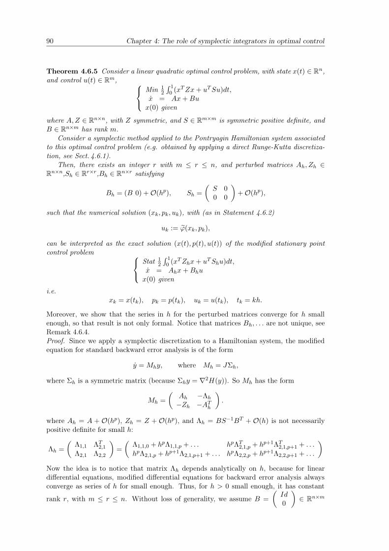
90 Chapter 4: The role of symplectic integrators in optimal control
Theorem 4.6.5 Consider a linear quadratic optimal control problem, with state x(t) ∈ Rn,and control u(t) ∈ Rm,
Min 12
∫ 10 (xT Zx + uT Su)dt,
x = Ax + Bux(0) given
where A, Z ∈ Rn×n, with Z symmetric, and S ∈ Rm×m is symmetric positive definite, andB ∈ Rn×m has rank m.
Consider a symplectic method applied to the Pontryagin Hamiltonian system associatedto this optimal control problem (e.g. obtained by applying a direct Runge-Kutta discretiza-tion, see Sect. 4.6.1).
Then, there exists an integer r with m ≤ r ≤ n, and perturbed matrices Ah, Zh ∈Rn×n,Sh ∈ Rr×r,Bh ∈ Rn×r satisfying
Bh = (B 0) + O(hp), Sh =
(S 00 0
)+ O(hp),
such that the numerical solution (xk, pk, uk), with (as in Statement 4.6.2)
uk := ϕ(xk, pk),
can be interpreted as the exact solution (x(t), p(t), u(t)) of the modified stationary pointcontrol problem
Stat 12
∫ 10 (xT Zhx + uT Shu)dt,
x = Ahx + Bhux(0) given
i.e.xk = x(tk), pk = p(tk), uk = u(tk), tk = kh.
Moreover, we show that the series in h for the perturbed matrices converge for h smallenough, so that result is not only formal. Notice that matrices Bh, . . . are not unique, seeRemark 4.6.4.Proof. Since we apply a symplectic discretization to a Hamiltonian system, the modifiedequation for standard backward error analysis is of the form
y = Mhy, where Mh = JΣh,
where Σh is a symmetric matrix (because Σhy = ∇2H(y)). So Mh has the form
Mh =
(Ah −Λh
−Zh −ATh
).
where Ah = A + O(hp), Zh = Z + O(hp), and Λh = BS−1BT + O(h) is not necessarilypositive definite for small h:
Λh =
(Λ1,1 ΛT
2,1
Λ2,1 Λ2,2
)=
(Λ1,1,0 + hpΛ1,1,p + . . . hpΛT
2,1,p + hp+1ΛT2,1,p+1 + . . .
hpΛ2,1,p + hp+1Λ2,1,p+1 + . . . hpΛ2,2,p + hp+1Λ2,2,p+1 + . . .
)
Now the idea is to notice that matrix Λh depends analytically on h, because for lineardifferential equations, modified differential equations for backward error analysis alwaysconverge as series of h for small enough. Thus, for h > 0 small enough, it has constant
rank r, with m ≤ r ≤ n. Without loss of generality, we assume B =
(Id0
)∈ Rn×m

4.6 Backward error analysis for optimal control problems? 91
and S = Id ∈ Rm×m. (Indeed, one can consider the change of coordinates for the controlu = S1/2u and x = Px where P ∈ Rn×n is a left inverse of the maximum rank matrixBS−1/2 ∈ Rn×m). We search for perturbed matrices Bh ∈ Rn×r and Sh ∈ Rr×r (diagonal)of the form
Bh =
(B1 0B2 B3
)=
(Id 00 0
)+ O(hp) Sh =
(Id 00 hpD
)
where D is a diagonal matrix with coefficients ±1 (thus D = D−1), so that
Λh = BhS−1h BT
h = BS−1BT + O(hp).
This identity is equivalent to
(Λ1,1 ΛT
2,1
Λ2,1 Λ2,2
)=
(B1B
T1 B1B
T2
B2BT1 B2B
T2 + h−pB3DBT
3
)
Matrix Λ1,1 is a perturbation of Id, so it is still positive definite. Therefore, one can take forB1 = Id+O(hp) the Cholesky decomposition of the positive definite matrix Λ1,1 = B1B
T1 .
For B2, one can take B2 = Λ2,1(BT1 )−1 = O(hp). Finally, for B3 = O(hp), we need
B3DBT3 = hp(Λ2,2 − B2B
T2 ) = O(h2p). For h small enough, this matrix has constant
rank, and this decomposition exists with a constant matrix D with coefficients ±1. Thisconcludes the proof. ¤
Conclusion
From the point of view of “geometric numerical integration” it is natural to use symplecticintegrators when solving Hamiltonian differential equations. This has been proved verysuccessful in many fields, in particular, in molecular dynamics simulations and in long-timeintegrations of planetary motion. For Hamiltonian systems arising form the Pontryaginmaximum principle in optimal control our conclusion is the following.
Due to the fact that one is concerned with boundary value problems, long-term in-tegration is not an issue. For integrations over short intervals, e.g. half a period of themotion of a planet, there is no real advantage of using a symplectic method. The solutionsof problems of Sects. 4.4 and 4.5 neither show a periodic or quasi-periodic behavior noran ergodic behavior like in molecular dynamics simulations. Therefore, no improvement ofsymplectic integrators can be expected, which is confirmed by numerical experiments.
For special problems, typically in low dimension and in situations where the Hamil-tonian is close to a critical value (Sect. 4.2), the structure preservation of symplecticintegrators is very important and symplectic methods can be much more efficient thannon-symplectic ones. Indeed, the theory of backward error analysis allows one to provethat the numerical solution of a symplectic method has the same qualitative behavior asthe exact flow. For example, in the integrable Martinet case, where the exact solution isperiodic, the numerical solution remains exponentially close to a periodic orbit, which ex-plains the excellent results, even on a relatively short interval of integration (a few periods).For non symplectic integrators, this structure is destroyed in general. We have shown thatbackward error analysis is possible for linear quadratic problems, involving the modifiedcontrol problem which are stationary point control problems, and not necessarily optimalcontrol problems (it depends on the signs of the eigenvalues of matrix Λh in the proof

92 Chapter 4: The role of symplectic integrators in optimal control
of Theorem 4.6.5). It is not clear whether this result can be extended also to non-linearproblems
Min∫ 10 g(x, u)dt
x = f(x, u)x(0) given.

Chapter 5
Splitting methods based on modified
potentials
Consider a system of ordinary differential equations
x = f(x), x(0) = x0 ∈ Rd
where the vector field f(x) is split as f(x) = A(x)+B(x), and the flows of A and B can beapproximated efficiently either exactly or with high-accuracy. Then, a standard approachfor this problem is to consider splitting methods of the form
eamhAebmhBeam−1hAebm−1hB · · · ea1hAeb1hB (5.1)
where ehA and ehB denote the flows associated to A and B. In the context of geometricintegration, this kind of integrator is of great interest because it preserve qualitative prop-erties of the exact solution. If A and B are two Hamiltonian vector fields, then all the flowseaihA and ebihB are symplectic, and the splitting method is symplectic as a composition ofsymplectic flows, which guaranties the well conservation of energy over exponentially longtimes.
A simple way to obtain high-order splitting methods is to use composition methods.One can consider as basic method the Strang splitting Φh = e
h2BehAe
h2B of order 2, and
then the associated standard composition methods of the form
Φγsh . . . Φγ1h (5.2)
of orders 4,6,8, involving respectively s = 5,9 and 17 compositions of the basic method, asdescribed in [HLW06] and as already used in Sect. 3.2. We shall consider these compositionsmethods in the numerical experiments as references for comparison.
A significant improvement, to reduce the number of compositions in (5.1), and thus thecomputational cost, is to consider processed methods. In order to reduce the number ofevaluations per step in the integration, the idea of processing, first introduced by Butcher[But69] in the context of Runge-Kutta methods, is to consider a composition of the form
eP ehKe−P .
where ehK is called the Kernel and should be cheap, and the order of eP ehKe−P , calledeffective order, is higher than that of ehK . Using a constant stepsize h, after N steps,we obtain eP (ehK)Ne−P . At first, we apply the processor (or corrector) e−P , then ehK
once per step, and the postprocessor eP is evaluated only when output is desired. The

94 Chapter 5: Splitting methods based on modified potentials
Kernel and the processor are taken as compositions of the flows associated to A, B whichmakes the splitting method symplectic for Hamiltonian vector fields. A general analysis ofsymplectic splitting methods with processing in given in [BCR99].
In practice, the main tool for the derivation of order conditions for splitting methodsis the Baker-Campell-Hausdorff (BCH) formula (see e.g. [HLW06, Sect. III.4.2]) whichimplies that the error for these methods is formally a linear combination of Lie bracketterms in the Lie-algebra generated by the vector fields A and B. For instance, for the LieTrotter splitting ehAehB, it yields
exp(hA) exp(hB) = exp(hA + hB + h2S2 + h3S3 + h4S4 + . . .) (5.3)
S2 =1
2[A, B]
S3 =1
12[A, [A, B]] +
1
12[B, [B, A]]
S4 =1
24[A, [B, [B, A]]]
To derive the order conditions for a splitting method (5.1) with unknown coefficientsai, bi, ci, . . ., one can apply repeatedly the BCH formula, this yields a system of polynomialequations in the coefficients of the splitting methods which can be solved numerically.
Now, assume that the vector field B is a small perturbation of vector field A, i.e.
B = O(ε)
where ε is a small parameter. Then, we obtain that Lie brackets involving few B’s arehigher than those with many B’s and should be canceled in priority to reduce the error ofthe method. For instance, [A, [A, B]] = O(ε) is dominant compared to [B, [B, A]] = O(ε2).The idea of processing has been applied to the symplectic integration of near-integrableHamiltonian systems in [WHT96, McL96].
An other improvement is possible for following special class of problems:
p = fA(p, q) + fB(q) (5.4)
q = gA(p, q)
where x = (p, q)T (p, q not necessarily of the same dimension) so that the flow associatedto B can be computed explicitly:
pn+1 = pn + hfB(qn), qn+1 = qn
and we assume the flow associated to A can be computed with high-accuracy efficiently.Consider the Lie Bracket C = [B, [B, A]]. A straightforward computation of vector fieldLie Brackets shows
C =
(fC
0
)where fC = fA
pp(fB, fB) − 2fB
q gAp fB.
Now, we assume that the derivatives fApp and gA
p are independent of p. This means thatfA(p, q) is (at most) quadratic in p and gA
p = 0 is (at most) linear in p. Then, the flow of C
can be integrated explicitly (similarly to fB), and the flows of B and C commute ([B, C] =0). It thus makes sense to compute the flow ebhB+βh3C associated to the vector fieldbhFB +βh3FC . Moreover, the brackets [B, . . . [B, [B, A]]] (with at least 3 B’s) all vanishes,which reduces significantly the number of order conditions. Notice that for Hamiltonian

5.1 Examples of splitting methods 95
vector fields A and B, the bracket C = [B, [B, A]] is also a Hamiltonian vector field. andthe corresponding Hamiltonian is given simply by the Poisson bracket B, B, A (seee.g. [HLW06] for details). A general study in this context is conducted in [BCR01], andalso [BCR00] in the situation of near integrable Hamiltonian systems, i.e. B = O(ε).Here, in addition to the term C = [B, [B, A]] they also consider additional terms like[B, [B, [A, [A, B]]]] as well as higher order terms.
In [BC05], they give an elegant elementary proof of the fact that any splitting method(or processed splitting method) with real coefficients of order greater or equal to three musthave a negative coefficient for A and also for B, as first shown in [GK96]. However, theyhighlight that this is not the case for splitting methods involving more general Lie bracketssince
eh6Be
h2Ae
2h3
B−h3
72Ce
h2Ae
h6B
has order 4 [Kos94], and the integrator
eh2AehB−h3
24Ce
h2A (5.5)
has effective order 4 [Row91, TI86], with positive coefficients ai, bi.These methods are called ‘Runge-Kutta Nyström methods’ in [BCR01] because they
were introduced in the context of second order differential equations x = f(x). However,the class of problems (5.4) includes not only second order differential equations like theN-body problems in Jacobi coordinates as studied in [WH91]. The main contribution ofthis chapter is to show that this method can also be successfully applied to asymmetricrigid body problems with an external potential. We also build a new processor for theTakahashi–Imada method (a modification of the Störmer-Verlet method), to achieve orderO(h10ε + h4ε2) (Sect. 5.2). Our numerical experiments indicate that this method is veryefficient for small ε when the cost of evaluating the vector field C = [B, [B, A]] togetherwith B is small compared to the cost of evaluating of A and B alone.
5.1 Examples of splitting methods
For the numerical solution of problems of the form (5.4), consider a splitting method ofthe form
ea1hAeb1hB . . . eanhAebnhB = ehK
or more generally,
ea1hAeb1hB+c1h3C . . . eanhAebnhB+cnh3C = ehK (5.6)
where C = [B, [B, A]]. Repeatedly applying the BCH formula (5.3), we obtain that themethod ehK is the exact flow of a linear combination in L(A, B) of nested Lie-Brackets,where L(A, B) is the free Lie algebra generated by the Lie operators associated to thevector fields A and B:
K = k1,1A + k1,2B + k2,1h[A, B] + k3,1h2[A, [A, B]] + k3,2h
2[B, [B, A]] + . . . (5.7)
= k1,1A + k1,2B +
∞∑
i=2
hi−1
d(i)∑
j=1
ki,jEi,j
where k1,1 = a1 + . . . an = 1 and k1,2 = b1 + . . . bn = 1 for consistent methods. Here, the
set Ei,jd(i)j=1 is a basis of the subspace Ln(A, B) generated by the independent brackets

96 Chapter 5: Splitting methods based on modified potentials
of order n, its dimension d(n) being 2, 1, 2, 3, 6 for n = 1 . . . 5 (see e.g. [BCR99]). Thesplitting method has order p if and only if K = A + B + O(hp), i.e. ki,jEi,j = 0 for all(i, j) with i = 2 . . . p. Notice that for symmetric splitting methods, ki,j = 0 for even i, i.ethe formal expansion of K in (5.3) is in even powers of h.
In our situation, for the special class of problems (5.4), all Lie brackets of the from[B, [. . . [B, A]]] with at least three B’s vanish, so the dimension of Ln(A, B) (and thus thenumber of order conditions) is reduced to d′(n) = 2, 1, 2, 2, 4 for orders n = 1 . . . 5.
5.1.1 Splitting methods without processing
A general study of splitting methods with processing is conducted in [BCR01], and also[BCR00] in the context of near integrable Hamiltonian systems, i.e. B = O(ε).
Example: a method of order 6 Solving order conditions (using MAPLE), we foundthat the minimal number of evaluations of A and B to get a symmetric method of order6 without processing, and involving terms of the form eahA and ebhB+ch3C is 4, and themethod is unique:
eb1hBeha1Aeb2hB+β2h3Cea2hAeb3hB+β3h3Cea2hAeb2hB+β2h3Cea1hAeb1hB (5.8)
and surprisingly, β1 = β5 = 0. In fact, this method was already derived in [OMF03].Since B = O(ε), the dominant terms of size O(ε) in (5.7) are the brackets E2,1 = [A, B],
E3,1 = [A, [A, B]], Ei,1 = [A, Ei−1] = O(ε) with only one A. Cancelling these terms in(5.7) allows to increase the accuracy for small ε.
Example: a new method of order O(h8ε + h6ε2) Next we searched for symmetricmethods of order O(h8ε + h6ε2). The idea is to vanish the coefficient k7,1 of the bracketE7,1 = [A, [A, [A, [A, [A, [A, B]]]]]] in the BCH formula. Numerically solving the orderconditions, we found a dozen of solutions. The one with minimal
∑i |ai| and positive bi is
eb1hB+β1h3Ceha1Aeb2hB+β2h3Ceha2Aeb3hB+β3h3Ceha3A (5.9)
eb3hB+β3h3Ceha2Aeb2hB+β2h3Ceha1Aeb1hB+β1h3C
a1 = a5 = 0.168735950563437422 b1 = b5 = 0.049086460976116245a2 = a4 = 0.377851589220928304 b2 = b4 = 0.264177609888976700a3 = −0.093175079568731453 b3 = 0.186735929134907054β1 = β5 = 0.00166171386175851684 β2 = β4 = −0.00461492847770001641β3 = 0.0000446959494108217
Notice that roundoff errors are proportional to max(∑
i |ai|,∑
i |bi|) ≥ 1. Here,∑
i |ai| ≈1.093 is quite small compared to standard splitting methods (5.1).
More generally, the next proposition gives a general formula to compute the coefficientski,1 of the brackets Ei,1 involving only one A. It is very similar to Proposition 2 in [LR01].
Proposition 5.1.1 Consider a splitting of the form (5.6). Then the coefficients ki,1, i =1, 2, 3, . . . of the brackets E11 = A, E21 = [A, B], Ei,1 = [A, Ei−1,1] (i ≥ 3), in the BCHexpansion (5.7) are given by the series expansion
γnt
eγnt − 1
n∑
k=1
bkeγkt =
∑
j≥0
kj+1,1tj
where γk = a1 + . . . + ak.

5.1 Examples of splitting methods 97
Proof. This is a consequence of the identity
ea1Ueb1V . . . eanUebnV = eW W = γnU +ad(γnU)
ead(γnU) − 1
n∑
k=1
bkead(γkU)V.
where ad(X)(Y ) = [X, Y ] (see [LR01, Prop. 2] for details). ¤
If the method splitting method is consistent then γn = 1 and the condition ki,1 = 0,i = 2 . . . p write
t
et − 1
n∑
k=1
bkeγkt = 1 + O(hp+1)
or equivalently, as shown in [McL95],
n∑
k=1
bkeγkt =
∫ 1
0etxdx + O(hp+1).
The solution of this problem which yields the highest order is known classically as the Gaussintegration formula. This permits the construction in [McL95] of a family of symmetricsplittings of the form (5.1) of orders O(hpε+h2ε2) with positive coefficients ai, bi. However,for small stepsize h, the error term O(h2ε2) becomes dominant. Therefore, these integratorsare improved in [LR01] to order O(hpε+h4ε2) in the context of the N-body Kepler problem,by performing a corrector term eβhC with C = [B, [B, A]] at each step.
Order O(h10ε+h4ε2) methods without processing For instance, the method denotedSBAB10 of order O(h10ε + h4ε2) proposed in [LR01] writes
eb11hB+h3βCea10hAeb10hB · · · ea1hAeb1hB+βh3C (5.10)
where the coefficients ai, bi are obtained from the weights of the Gauss-Lobatto formula.It is the unique method of the form (5.10) with positive coefficients ai and bj (see [LR01,Table I]).
5.1.2 Splitting methods with processing
We give here examples of splitting methods with processing. Our numerical experiments(see further) indicate that processed splitting methods are more efficient in general thanunprocessed methods.
Order O(h6ε) methods with processing In [BCR01] families of 6 and 8-order splittingmethod with processing are introduced. The method 6 : ABA − 3, 6; 3 of order 6 has theform
eP ea1hAeb1hBea2hAeb2hB+c2h3Cea2hAea1hAeb1hBe−P (5.11)
where eP is the processor composed of explicitly computable flows involving terms of thethe type as the Kernel. They also investigate the use of higher order terms like D =[B, B, A, A, B], E = [B, A, B, B, A, A, B], F = [B, B, B, A, A, A, B] and build the methoddenoted (6 : ABA − 3, 6; 7) of order 6
eP ea1hAeb1hBea2hAeb2hB+c2h3C+e2h7E+f2h7F ea2hAea1hAeb1hBe−P (5.12)
where eP is a processor (see [BCR01, Table 2] for the coefficients of these two methods).

98 Chapter 5: Splitting methods based on modified potentials
Order O(h6ε + h4ε2) method with processing In [BCR00], new processed splittingmethods of orders 3, 4, 5 for perturbed Hamiltonian systems are introduced. For instance,the first method in [BCR00, Table V] is a processor for method (5.5) of order O(h6ε+h4ε2).
The next proposition states that by using the processing technique, it is always possibleto cancel the terms ki,jEi,1 of size O(ε), ie. the brackets [A, . . . A, B]. This result, true forany splitting method, is originally due to [WHT96].
Proposition 5.1.2 Consider a splitting method ehK of the form (5.7) and assume it hasorder O(hα1ε + hα2ε2 + . . . + hαkεk) for B = O(ε). Consider a processor eP of the form
P =∞∑
i=2
hi
d(i)∑
j=1
pi,jEi,j .
Then, for pi−1,1 = ki,1, i = 2 . . . p, the processed method eP ehKe−P has order O(hpε +hα′
2ε2 + . . . + hα′
kεk).
Proof. The idea is to notice that the coefficient of Ei,1 in the BCH expansion of eP ehKe−P
is simply ki,1 − pi−1,1. ¤
5.2 Processed Takahashi–Imada splitting method
Consider the Takahashi–Imada method of effective order 4, as introduced in [Row91, TI86],
eh2B−h3
48CehAe
h2B−h3
48C .
Notice that in the particular case of a Hamiltonian system with Hamiltonian H(p, q) =12pT p + U(q), this method simply writes
pn+1/2 = pn − h
2
(I − βh2∇2U(qn))∇U(qn)
qn+1 = qn + hpn+1/2
pn+1 = pn+1/2 −h
2
(I − βh2∇2U(qn+1))∇U(qn+1)
with β = 1/12. It can be interpreted as the Störmer–Verlet method applied with themodified potential U = U − β
2 h2‖∇U‖2.Using the techniques presented in the previous section, we present in this section the
construction of a family of processors to achieve effective orders O(hpε + h4ε2) for arbi-trary p.
For the Takahashi–Imada method, Proposition 5.1.1 with n = 2 yields the series
t
1 − et
(1
2e0 +
1
2et
)=
t
2+
t
et − 1= 1 +
∞∑
j=2
Bj
j!tj = 1 +
t2
12− t4
720+ . . .
where the B′js are the Bernoulli numbers. Now, we consider a processor of the same form
as in Proposition 5.1.1, with γn = a1 + . . . + an = 0 and b1 + . . . + bn = 0, so the termγnt
eγnt−1 has to be replaced by 1. To achieve order p, the condition pi−1,1 = ki,1, i = 2, . . . pis equivalent to
1 + tn∑
k=1
bkeγkt =
t
2+
t
et − 1+ O(tp)

5.3 Applications to mechanical problems 99
or alson−1∑
k=1
bk(γk)i−1 =
Bi
i, i = 2, . . . p − 1
Notice that for arbitrary distinct γi’s, and n = p − 1, this system of equation is a squareVandermonde linear problem for coefficients bk’s which possesses a unique solution.
One solution of this system with p = 10 is given by the following new processor for theTakahashi–Imada method. It yields a processed method of order O(h10ε + h4ε2).
eP = ea1hAeb1hB+c1h3Cea2hAeb2hB · · · ea8hAeb8hBea9hAec2h3C
a1 = a9 = −5/4, a2 = a8 = 1/8, a3 = a7 = 1/4, a4 = a6 = 1/2, a5 = 3/4
d1 = −d8 = 0.041139583138698574 d2 = −d7 = −0.108267614767371103
d3 = −d6 = 0.135191882308478947 d4 = −d5 = −0.238887935991110594
c1 = −1/900 c2 = −0.014597270750786141
Moreover, c1, c2 are chosen so that the brackets [A, B, B, A] and [A, A, B, B, A] of sizeO(ǫ2) in the BCH expansion of eP ehKe−P vanishes. Thus, the dominant error term in thelocal error is given by
eP ehKe−P − ehA+hB =h5
1440[B, A, A, A, B] + O(h11ε + h5ε3).
Notice that this dominant error term cannot be reduced by processing, because the coef-ficient for [B, A, A, A, B] equals 1/360 − p21/12 + p2
21/2 − p41 = 11440 , where parameters
p21 = 1/12 and p41 = −1/720 are already used to cancel the brackets E31, E51.
Remark 5.2.1 Similarly to the simplified Takahashi–Imada method proposed in [WHT96]and as studied in [HMS08], a possibility to avoid the derivative evaluation fB
q (q) of thevector fields fB(q) is to replace
(Id−2βh2gA
p fBq (q)
)fB(q) by f
(q−2βh2gA
p fq(q))
and thusconsider the approximation
fB(q) + βh2fC(q) = fB(q − 2βh2gAp fB
q (q)) + βh2fApp
(fB(q), fB(q)
)+ O(ε3h4)
This approximation of fB(q) + βh2fC(q) requires only two evaluations of fB(q). We givehere some consequences of the analysis in [HMS08] in our context of perturbed Hamiltoniansystem integration. This simplification used for the Kernel of the processed Takahashi–Imada integrator still yields a symmetric and reversible integrator, with effective orderO(hpε + h4ε2), and it is still volume preserving (because a map (p, q) 7→ (p + a(q), q) isalways volume preserving), However, as shown in [HMS08, Sect. 4], the modified methodit is no longer symplectic. In general, without any particular assumption on the potential,this adds a linear drift in the energy, of size O(tε3h4).
Notice that the considered simplification can be successfully applied to the processorseP and e−P alone, and the energy error will remain bounded with size O(hpε + ε2h4) onexponentially long-time intervals, because the processed integrator is still conjugate to asymplectic integrator.
5.3 Applications to mechanical problems
5.3.1 The N-body problem in Jacobi coordinates.
We consider the N -body problem with Hamiltonian,
H(p, q) =1
2
N∑
i=0
1
mipT
i pi − G
N∑
i=1
i−1∑
j=0
mim0
‖qi − q0‖

100 Chapter 5: Splitting methods based on modified potentials
As proposed in [WH91], the Hamiltonian can be split as H = HA+HB where HA representsthe integrable Keplerian part, corresponding to the interactions Sun-planets, and the Bpart is a small perturbation, corresponding to the interactions between the planets. Theuse of Jacobi coordinates makes HB depend only on the positions of the planets (see e.g.[Mey99, Sect. 3.5] for a presentation of Jacobi coordinates), and thus easy to integrate(explicit).
The integrable part A corresponds to (N − 1) decoupled two-body Kepler problemswhich can be solved exactly using the Kustaanheimo-Stiefel transformation (1965) (seeAppendix C for details). The B part can be integrated explicitly (see below).
We detail the integration for the 3 body problem Sun-Jupiter-Saturn. Let m0, m1, m2,q0, q1, q2 and p0, p1, p2 denote respectively the masses, the positions and momenta of theSun, Jupiter and Saturn. We assume m0q0 + m1q1 + m2q2 = 0 (center of mass is at theorigin) and p0 + p1 + p2 = 0 (total momentum).
Introducing the Jacobi coordinates Q1, Q2, and P1, P2,
Q1 = q1 − q0 Q2 = q2 − (α0q0 + α1q1)
P1
M1=
p1
m1− p0
m0
P2
M2=
p2
m2− p0 + p1
m0 + m1
with scalars α0 = m0m0+m1
, α1 = m1m0+m1
and masses M1 = m0m1m0+m1
, M2 = (m0+m1)m2
m0+m1+m2, then
the Hamiltonian becomes H = HA + HB, where
HA =( P 2
1
2M1− Gm1m0
‖Q1‖)
+( P 2
2
2M2− Gm2m0
‖Q2‖)
HB = Gm2m0
( 1
‖Q2‖− 1
‖Q2 + α1Q1‖)− Gm1m2
‖Q2 − α0Q1‖
Since the Sun is the heaviest body, we have α1 = O(ε) and B = O(ε). For the Solarsystem, we have approximately ε ≈ 10−3.
100 101
10−12
10−9
10−6
10−3Hamiltonian error
cpu time
Figure 5.1: Three body problem Sun-Jupiter-Saturn. Comparison of Hamiltonian errorversus cpu time for various splitting methods. Without processing: Strang splitting andcomposition methods (5.2) of orders O(hpε), p = 2, 4, 6, 8 (dotted lines), method (5.10)order O(h10ε + h4ε2) (dashed lines). With processing: methods (5.5) and (5.11) of ordersO(h6ε+h4ε2) and O(h6ε) (dashed-dotted lines), new method (Sect. 5.2) of order O(h10ε+h4ε2) (solid line).

5.3 Applications to mechanical problems 101
Numerical experiment We consider the 3-body problem Sun-Jupiter-Saturn with theinitial data given in [HLW06, Table I.2.2]. We integrate on the interval of days [0, 108] andmany stepsizes (e.g. h = 400 · 2−j/4, j = 1 . . . 20 for the Strang splitting). In Figure 5.1,we plot the relative Hamiltonian error as a function of the cpu times of computation. Weobserve that the preprocessed methods are the most efficient. For the processed Takahashi–Imada method of order O(h10ε+h4ε2) with observe a line with slop p = 10. This indicatesthat the second error term of size O(h4ε2) is negligible in this numerical experiment.
5.3.2 The motion of a rigid body with an external potential.
In the presence of an external potential V (Q), the motion of a rigid rigid body, relative toa fixed coordinate system, is determined by a Hamiltonian system constrained to the Liegroup SO(3) and the Hamiltonian is
H(y, Q) =1
2
(y21
I1+
y21
I2+
y21
I3
)+ V (Q)
where the constants I1, I2, I3 are the moments of inertia, y(t) = (y1(t), y2(t), y3(t)) is theangular momentum and Q(t) is the orthogonal matrix that gives the orientation of therigid body in the fixed frame (see Chapter 3). The equations of motion are
y = y I−1y + f(Q), Q = Q I−1y,
where I = diag (I1, I2, I3) and the hatmap notation y is defined already in (3.2),
y =
y1
y2
y3
, y =
0 −y3 y2
y3 0 −y1
−y2 y1 0
.
The torque is given by
f(Q) = −rot (QT ∂V
∂Q)
where∂V
∂Q=
(∂V
∂Qij
)
i,j=1...3
∈ R3×3
is the Jacobian matrix. Here, for all 3 × 3 matrix M ,the vector rotM in R3 is defined by
rotM = M − MT . (5.13)
A standard approach to solve this problem is to split it into the free rigid body motion
A : y = y I−1y, Q = Q I−1y,
which can be solved using e.g. the high-order preprocessed DMV, plus a torqued motion,
B : y = f(Q), Q = 0,
It can be easily verified that this problem is in the form (5.4). A direct computation shows
fC(Q) = 2fB(Q)I−1fB(Q) − 2∂fB(Q)
∂Q(Q I−1fB(Q))
We consider two different external potentials.

102 Chapter 5: Splitting methods based on modified potentials
5.3.2.1 Asymmetric heavy top
We consider an asymmetric rigid body and we assume the center of gravity to be (0, 0, 1)in the body frame, and that the third coordinate is the stationary frame is vertical. Thepotential energy for gravity is given by (see e.g. [HLW06, Sect. VII.5.3.(II)])
V (Q) = εQ33.
The torques corresponding to the brackets C = [B, [B, A]], D, . . ., reduce to polynomi-als in Q31, Q32, Q33,
fB(Q) = ε(Q32,−Q31, 0)T
fC(Q) = ε2(Q32Q33
I1,−Q31Q33
I2, 0)T
fD(Q) = 2ε3
+ 2I21Q32Q
233 − 1
I21Q3
32 − 1I22Q2
31Q32
− 2I22Q31Q
233 + 1
I22Q3
31 + 1I21Q31Q
232
( 2I22− 2
I21)Q31Q32Q33
and similar formulas for fE(Q) and fF (Q). It requires to compute at each step the compo-nents Q31, Q32, Q33 from the quaternion q = (q0, q1, q2, q3) representing the rotation matrixQ,
Q31 = −2q0q2 + 2q1q3 Q32 = 2q0q1 + 2q2q3 Q33 = q20 − q2
1 − q22 + q2
3.
All constants depending on the moments of inertia I1, I2, I3 can be computed only once.Thus, the cost of evaluating altogether fB(Q), fC(Q), fD(Q), fE(Q) is negligible comparedto the resolution of the free rigid body part.
Numerical experiment In Figure 5.2 with consider a rigid body with moments ofinertia I1 = 0.345, I2 = 0.653, I3 = 1.0, which corresponds to the water molecule, andwe integrate on the interval [0, 100]. The initial condition for the angular momentum isy1(0) = 1.8, y2(0) = 0.4, y3(0) = −0.9 and we take Q(0) = Id.
We compare the relative Hamiltonian error versus the number of evaluations of the freerigid body part eA (which clearly dominates the cost) for various sizes ε of the gravitytorque. Again we observe that the processed methods are very efficient. For small ε, weobserve for the processed Takahashi–Imada method of order O(h10ε + h4ε2) (solide line)a line op slop p = −10 for large stepsize and a line of slop p = −4 for small stepsizes.Indeed, for ε → 0, the error term O(h4ε2) becomes negligible compared to O(h10ε), andthe efficiency of the method gets better and better.
5.3.2.2 Motion of a satellite
We consider the simplified model describing the motion of a satellite is a circular orbitaround the Earth considered in [Mit00, LLM06]. The numerical integration of this problemis discussed in [CFSZ08]. For this problem, the potential, due to the action of the earthon the satellite, is quadratic in Q,
V (Q) =ε
2(QT e3)
T (IQT e3) =ε
2
(I1Q
231 + I2Q
232 + I3Q
233
)
where e3 = (0, 0, 1)T . The torques are
fB(Q) = εx × (Ix) where x = (QT e3),
fC(Q) = 2fB(Q) × (I−1fB(Q)) + 2ε(x × (Iy) + y × (Ix)) where y = (I−1fB) × x,
and similarly for fD(Q).

5.3 Applications to mechanical problems 103
102 103 104 105 106
10−15
10−12
10−9
10−6
10−3
102 103 104 105 106
10−15
10−12
10−9
10−6
10−3
102 103 104 105 106
10−15
10−12
10−9
10−6
10−3
102 103 104 105 106
10−15
10−12
10−9
10−6
10−3
Hamiltonian error
ε = 100
evaluations
Hamiltonian error
ε = 10−2
evaluations
Hamiltonian error
ε = 10−3
evaluations
Hamiltonian error
ε = 10−4
evaluations
Figure 5.2: Asymmetric heavy top problem. Comparison of Hamiltonian error versusnumber of evaluations of ehA and ehB for various splitting methods. Without processing:Strang splitting and composition methods (5.2) of orders O(hpε), p = 2, 4, 6, 8 (dottedlines), method (5.9) order O(h8ε + h6ε2) (dashed lines). With processing: methods (5.11)and (5.12) of order O(h6ε) (dashed-dotted lines), new method (Sect. 5.2) of order O(h10ε+h4ε2) (solid line).
Numerical experiment In Figure 5.3 with consider a rigid body with moments ofinertia I1 = 0.6, I2 = 0.8, I3 = 1.0, which corresponds to an asymmetric body, and weintegrate on the interval [0, 100]. The initial condition for the angular momentum is y1(0) =1.8, y2(0) = 0.4, y3(0) = −0.9 and we take Q(0) = Id. The numerical are very similar asfor the heavy top problem in the previous section. Again, the processed methods are themost efficient.
5.3.3 Molecular dynamics simulation: dipolar soft spheres
Splitting algorithm for multi-rigid body dynamics have been studied in [DLM97, BCF01].We consider a molecular dynamics simulation where the molecule are described by dipolarsoft sphere, as described in [DLM97, Appendix A]. This problem is also considered in[CFSZ08] as a numerical illustration for rigid body integrators. This model model can beused to study water and aqueous solutions, as water can be modeled by small dipoles.
We consider N molecules with mass m, positions qi ∈ R3, orientations Qi ∈ SO(3),linear momenta pi ∈ R3 and angular momenta yi ∈ R3. The Hamiltonian for this problemis
H(y, p, Q, q) = T (y, p) + V (Q, q)

104 Chapter 5: Splitting methods based on modified potentials
102 103 104 105 106
10−15
10−12
10−9
10−6
10−3
102 103 104 105 106
10−15
10−12
10−9
10−6
10−3
Hamiltonian error
ε = 100
evaluations
Hamiltonian error
ε = 10−3
evaluations
Figure 5.3: Motion of a satellite. Comparison of Hamiltonian error versus number ofevaluations of ehA and ehB for various splitting methods. Without processing: Strangsplitting and composition methods (5.2) of orders O(hpε), p = 2, 4, 6, 8 (dotted lines),method (5.10) order O(h10ε + h4ε2) (dashed lines). With processing: methods (5.5) and(5.11) of orders O(h6ε + h4ε2) and O(h6ε) (dashed-dotted lines), new method (Sect. 5.2)of order O(h10ε + h4ε2) (solid line).
where
T (y, p) =1
2
N∑
i=1
(p2i,1 + p2
i,2 + p2i,3
m+
y2i,1
I1+
y2i,2
I2+
y2i,3
I3
)
is the sum of the translational and rotational kinetic energies of each rigid body. Weconsider an inter-body potential V (Q, q) of the form
V (Q, q) =∑
1≤i<j≤N
Vi,j(Qi, qi, Qj , qj)
where the interaction between particle i and particle j has the form
Vi,j = εV shorti,j + εV dip
i,j
V shorti,j = 4r−12
i,j ri,j = ‖qi − qj‖V dip
i,j = r−3i,j µT
i µj + 3r−5i,j µT
i (qi − qj)µTj (qj − qi).
Here, the term V shorti,j corresponds to a repulsive short range interaction, while V dip
i,j modelsthe dipole interaction which depends on the dipole vector orientations µi ∈ R3 given by
µi = Qiµi
for some fixed reference orientations µi ∈ R3.The problem can be split as
yi = yiI−1yi
pi = 0
Qi = QI−1yi
qi = pi
m
yi = −rot (QTi
∂V∂Qi
)
pi = −∂V∂qi
Qi = 0qi = 0
i = 1 . . . N.
where the operator rot is defined in (5.13). The vectors
vi = rot (QTi
∂V
∂Qi) = ε
∑
j 6=i
aij and wi =∂V
∂qi= ε
∑
j 6=i
bij (5.14)

5.3 Applications to mechanical problems 105
can be computed straightforwardly using
aij =3∑
k=1
αijk2Qik3 − αijk3Qik2
αijk3Qik1 − αijk1Qik3
αijk1Qik2 − αijk2Qik1
, αijkl =
∂Vi,j
∂Qikl
= r−3i,j µilµjk + 3r−5
i,j γjiµilq(k)ij ,
bij =(− 48r−14
ij − 3r−5i,j µT
i µj − 15r−7i,j γijγji
)qij + 3r−5
i,j γjiµi − 3r−5i,j γijµj ,
where we use the notations
qij = qi − qj γij = µTi (qi − qj), (5.15)
and q(k)ij is the kth component of vector qij .
Computation of fC Consider the vector fields fA, gA, fB given by
fAi =
(yiI
−1yi
0
)gAi =
(QiI−1yi
pi
m
)fB
i =
(−rot (QT
i∂V∂Qi
)
−∂V∂qi
)i = 1 . . . N.
Then, vector field fC is given by
fCi (Q, q) =
∂2fAi
∂(y, p)2(fB, fB) − 2
∂fBi
∂(Q, q)
∂gA
∂(y, p)fB
=
(2viI
−1vi − 2ε∑
j 6=i ci,j
−2ε∑
j 6=i di,j
)
where the vectors vi are given in (5.14) and the vectors cij , dij can be computed as follows.
cij =3∑
k=1
βijk2Qik3 − βijk3Qik2 + αijk2Qik3 − αijk3Qik2
βijk3Qik1 − βijk1Qik3 + αijk3Qik1 − αijk1Qik3
βijk1Qik2 − βijk2Qik1 + αijk1Qik2 − αijk2Qik1
βijkl = r−3i,j µilµjk − 3r−5
i,j µTj qijµilq
(k)ij
+3
mr−5i,j µil
((µjk + 5r−2
i,j γjiq(k)ij
)qTijwji + µT
j wjiq(k)ij − γjiwjik
)
dij = 3r−5ij
(− µT
i µj − µTj µi + 5r−2
ij γijµTj qij − 5r−2
ij γjiµTi qij
+ 5r−2ij
m(γjiw
Tjiµi − γijw
Tjiµj)
+r−2ij
mqTijwji((−224r−9
ij − 5µTi µj − 35r−2
ij γijγji)))qij
+ 3r−5ij
(− µT
j qij +1
mµT
j wji + 5r−2ij
mqTijwjiγji
)µi
+ 3r−5ij
(− µT
i qij +1
mµT
i wji − 5r−2ij
mqTijwjiγij
)µj
+ 3r−5ij γjiµi − 3r−5
ij γijµj
+ 3r−5ij
m
(16r−9
ij + µTi µj + 5r−2
ij γijγji
)wji

106 Chapter 5: Splitting methods based on modified potentials
We have used the following notations
wij = wi − wj , Qi = QiI−1vi, µi = Qiµi
where vi and wi are given in (5.14) and qij , q(k)ij , γij are given in (5.15).
100 101 102
10−12
10−9
10−6
10−3
100 101
10−12
10−9
10−6
10−3
Hamiltonian error
ε = 100
cpu time
Hamiltonian error
ε = 10−2
cpu time
Figure 5.4: Molecular dynamics simulation: dipolar soft spheres. Comparison of Hamil-tonian error versus cpu time for various splitting methods. Without processing: Strangsplitting and composition methods (5.2) of orders O(hpε), p = 2, 4, 6, 8 (dotted lines),method (5.10) order O(h10ε + h4ε2) (dashed lines). With processing: methods (5.5) and(5.11) of orders O(h6ε + h4ε2) and O(h6ε) (dashed-dotted lines), new method (Sect. 5.2)of order O(h10ε + h4ε2) (solid line).
Numerical experiment We integrate in the interval [0, 5]. Similarly to the numericalexperiments in [CFSZ08], we take 125 particles with initial positions qi(0) the points withinteger coordinates of the cube [0, 4]3 in R3, and initial velocities pi(0) zero. The angularmomentum yi(0) and the orientations of each particle is chosen randomly with a quaternionwith random components in [−1, 1]. We take m = 1, the moments of inertia of the rigidbodies are I1 = 0.345, I2 = 0.653, I3 = 1.0 corresponding water molecules, and the fixedorientations for the dipoles are µi = (0, 1, 1)T .
For this problem, the processed method (5.11) of [BCR01] is more efficient than theprocessed Takahashi–Imada. An explanation is the following. The cost of computing f A
is O(N), linear with the number of particles, whereas the cost of the torque fB growsquadratically O(N 2), and thus dominates the cost. Our numerical experiments indicatethat the computation of fB together with fC costs about 3 times the computation of fB
alone. Unlike previous problems considered in this chapter, this is far from negligible.Method (5.11) and the processed Takahashi–Imada method both require one evaluation offC per step. Method (5.11) requires 3 evaluations of fB , thus the relative overcost due tothe expensive evaluation of fC is about 2/3 ≈ 0.66%, whereas the processed Takahashi–Imada method requires one evaluation of fB so the relative overcost is about 200%.

Chapter 6
Splitting methods with complex
times for parabolic equations
Note: This chapter is identical to the article [CCDV08] in collaboration with F. Castella,P. Chartier and S. Descombes.Similar results are derived independently by E. Hansen & A. Ostermann in [HO08b].
Although the numerical simulation of the heat equation in several space dimensions isnow well understood, there remain a lot of challenges in the presence of an external source,e.g. for reaction-diffusion problems, or more generally for the complex Ginzburg-Landauequation.
Reaction-diffusion equations are mathematical models that describe how the populationof one or several species distributed in space evolves under the action of two concurrentphenomena:
– “reactions” between species in which predators eat preys;
– diffusion which makes the species spread out in space.
Apart from biology and ecology, systems of this sort also appear in chemistry (hence theterm reaction), geology and physics. From a mathematical point of view, they belong tothe class of semi-linear parabolic partial differential equations and can be represented inthe general form
∂u
∂t= D∆u + F (u),
where each component of the vector u(x, t) ∈ Rd represents the population of one species,D is the matrix of diffusion coefficients (often diagonal) and F accounts for all local inter-actions between species. The solutions of reaction-diffusion equations display a wide rangeof behaviours, like traveling waves and wave-like phenomena, or dissipative solitons.
The most simple reaction-diffusion equation occurs in chemistry and involves the con-centration u of a single reactant in one spatial dimension,
∂tu = D∂2xu + F (u), (6.1)
is also referred to as the KPP (Kolmogorov-Petrovsky-Piscounov [KPP37]) equation. Ifthe reaction term vanishes, then the corresponding equation is the heat equation. Specificforms of this one-dimensional reaction-diffusion equation appear in the litterature:

108 Chapter 6: Splitting methods with complex times for parabolic equations
– the choice F (u) = u(1−u) yields Fisher’s equation and is used to describe the spreadingof biological populations;
– the choice F (u) = u(1 − u2) describes Rayleigh-Benard convection;
– the choice F (u) = u(1 − u)(u − α) with 0 < α < 1 arises in combustion theory and isreferred to as Zeldovich equation.
Two-component (and more) systems are also possible and allow for a much larger range ofpossible phenomena than their one-component counterparts. They can be represented inthe following form
∂tu1...
∂tud
=
D1
. . .Dd
∆u1...
∆un
+
F1(u1, . . . , ud)...
Fd(u1, . . . , ud)
Even more generally, the diffusion operator may involve a complex number: we shalldenote Re z the real part, Im z the imaginary part, and arg z ∈] − π, π] the argument of acomplex number z. In this case, we obtain a complex Ginzburg-Landau equation with apolynomial non-linearity of the form
∂u
∂t= δ∆u −
K∑
j=0
µj |u|2ju (6.2)
where K ≥ 1 is an integer, δ and µj , j = 1 . . .K, are complex numbers with Re δ > 0, andReµK > 0. For example, when K = 1, we obtain the well-known cubic Ginzburg-Landauequation [FT88], and when K = 2, the equation given by Fauve-Thual in [6] as a model oflocalized structures generated by subcritical instabilities.
When one wishes to approximate the solution of the above parabolic non-linear problem(6.1) or (6.2), a method of choice is based on operator-splitting: the idea is to split theabstract evolution equation (6.1) (or (6.2)) into two parts which can be solved explicitlyor at least approximated efficiently.
For the sake of simplicity, let us illustrate the method on the linear case
∂u
∂t= ∆u + V u, (6.3)
where V is a linear operator, say V u = v(x)u with v(x) a smooth function. Splittingmethods basically rely on the identity
eh(∆+V ) = eh∆ ehV + O(h2
),
or on higher order approximations obtained by combining eh∆ and ehV in the appropriatefashion. Dividing time t into n time steps of size h (where t = nh), the above approximationindeed leads to the equality
u(t) = et(∆+V ) u(0) = enh(∆+V ) u(0) =(eh∆ ehV
)nu(0) + O(h).
The extension to the non-linear case is straightforward, replacing ehV by the flow of anonlinear differential equation.
For a positive stepsize h, the most simple numerical integrator is the Lie-Trotter split-ting
ehV eh∆ (6.4)

109
which is an approximation of order 1 of the solution of (6.3), while the symmetric version
eh/2 V eh∆eh/2 V (6.5)
is referred to as the Strang splitting and is an approximation of order 2. For higher orders,one can consider general splitting methods of the form
eb1hV ea1h∆eb2hV ea2h∆ . . . ebshV eash∆. (6.6)
The number of order conditions can be significantly reduced by imposing the symmetryas = 0 and aj = as−j , bj = bs+1−j whenever 1 ≤ j ≤ s. It is interesting to note that raisingthe order can also be achieved by considering composition methods of the form
Ψh := Φγsh . . . Φγ1h, (6.7)
where Φh is a low order approximation. Symmetry can even be obtained by imposingγj = γs+1−j (1 ≤ j ≤ s), and by choosing Φh symmetric. For instance, when Φh is theStrang splitting (6.5), this approach leads to
Ψh = ehγs/2 V ehγs∆eh(γs+γs−1)/2 V ehγs−1∆ . . . ehγ1∆ehγ1/2 V .
However, achieving higher order is not as straightforward as it looks. A disappointingresult indeed shows that all splitting methods (or composition methods) with real coeffi-cients must have negative coefficients ai and bi in order to achieve order 3 or more. Theexistence of at least one negative coefficient was shown in [She89, SW92], and the existenceof a negative coefficient for both operators was proved in [GK96]. An elegant geometricproof can be found in [BC05]. As a consequence, such splitting methods cannot be usedwhen one operator, like ∆, is not time-reversible.
In order to circumvent this order-barrier, there are two possibilities. One can usea linear, convex combination (see [GRT02, GRT04, BDL06] for methods of order 3 and4) or non-convex combination (see [Sch02, Des01] where an extrapolation procedure isexploited), of elementary splitting methods like (6.6). Another possibility is to considersplitting methods with complex coefficients ai and bi with positive real parts (see [Cha03]in celestial mechanics). In 1962/1963, Rosenbrock [Ros63] considered complex coefficientsin a similar context.
In this article, we consider splitting methods of the form (6.7), and we derive newhigh-order methods using composition techniques originally developed for the geometricnumerical integration of ordinary differential equations [HLW06]. The main advantages ofthis approach are the following:
– the splitting method inherits the stability property of exponential operators;
– we can replace the costly exponentials of the operators by cheap low order approxima-tions without altering the overall order of accuracy;
– using complex coefficients allows to reduce the number of compositions needed to achieveany given order;
This paper is organized as follows. In Sect. 6.1, we derive new high-order splittingmethods. In Sect. 6.2 we give a rigorous order estimate in the linear case, obtained asa direct consequence of the recent results by Hansen & Ostermann [HO08a]. Sect. 6.3presents several numerical simulations, confirming the formally expected order of accuracyin the non-linear case.

110 Chapter 6: Splitting methods with complex times for parabolic equations
6.1 Composition methods
Composition methods were mainly developed in the the 90’s in the papers of Suzuki [Suz90],Yoshida [Yos90] and McLachlan [McL95] in the context of ordinary differential equations.In the classical theory, only real coefficients γ1, . . . , γs were considered. In this section, weconstruct new composition methods, involving complex coefficients.
The idea is to compose with different stepsizes a basic one-step method Φh of low orderof accuracy. Given the scalars γ1, . . . , γs, the corresponding composition method is definedas
Ψh = Φγsh . . . Φγ1h (6.8)
with stepsizes γ1h, γ2h, . . . , γsh.For the method Φh, the simplest choice is the symmetric Strang splitting
Φh = eh/2 V eh∆eh/2 V .
Then, we obtain the splitting method
Ψh = ehγs/2 V ehγs∆eh(γs+γs−1)/2 V ehγs−1∆ . . . ehγ1∆ehγ1/2 V
Another possibility, to avoid computing the exact flow eh∆, is to replace it by a symmetricapproximation, e.g. the Crank-Nicholson discretization (which is equivalent to the implicitmidpoint rule for linear systems)
ΦMh =
(Id − h
2∆
)−1 (Id +
h
2∆
).
One can also discretize the flow ehV of the reaction, and consider the cheaper basic sym-metric method
Φh = ΦIh/2 ΦM
h ΦEh/2 (6.9)
where ΦEh denotes the flow of the explicit Euler method yn+1 = yn+hf(yn) and ΦI
h denotesthe flow of the implicit Euler method yn+1 = yn + hf(yn+1) for the approximation of thereaction. This is the Peaceman-Rachford formula [PJ55] originally developed for the heatequation, and extended to reaction-diffusion problems in [DR03].
Focusing back to composition methods, their construction relies on the following clas-sical result in geometric integration.
Theorem 6.1.1 (see [HLW06, Theorem II.4.1]) Let Φh be a method of (classical) orderp. If
γ1 + . . . + γs = 1 γp+11 + . . . + γp+1
s = 0, (6.10)
then composition method (6.7) has (classical) order p + 1.
Proof. The idea of proof is to show that if the basic method has order p,
Φh(y) = ϕh(y) + C(y)hp+1 + O(hp+2),
where ϕh denotes the exact flow, then
Φγsh . . . Φγ1h(y) = ϕh(y) + C(y)(γp+11 + . . . + γp+1
s )hp+1 + O(hp+2).
¤

6.1 Composition methods 111
6.1.1 Triple Jump composition methods with real coefficients
Using only real coefficients, equations (6.10) have no real solution for odd p, so the orderincrease is only possible for even p. In this case, the smallest s which allows for the existenceof a solution is s = 3. If we impose symmetry, γ1 = γ3 and we obtain a unique solution
γ1 = γ3 =1
2 − 21/(p+1), γ2 = − 21/(p+1)
2 − 21/(p+1). (6.11)
If the basic method Φh is symmetric of order p (p even), then we reach order p + 1, butdue to the symmetry of the method the order is in fact p + 2. Now, this procedure can berepeated up to any order: we start with a symmetric method of order 2, we apply (6.11)with p = 2 to obtain order 4. With this new method, we repeat (6.11) with p = 4 to obtaina symmetric composition method of order 6 with 9 stages and so on.
These methods are originally due to Creutz & Gocksch [CG89], Forest [For89], Suzuki[Suz90], Yoshida [Yos90]. The name ‘Triple Jump composition methods’ was given in[HLW06, Example II.4.2]. However, since γ2 < 0, these methods cannot be applied tonon-reversible problems. In addition, the estimate |γj | > 1 implies a terrible zig-zag inthe coefficients of the methods. Thus, this technique is not very efficient in the contextof ordinary differential equations, and to reach high order it is much better to resort togeneral composition methods by directly solving the p-order conditions for large p.
6.1.2 Triple Jump composition methods with complex coefficients
For s = 3, equation (6.10) possesses p + 1 solutions in C,
γ1 = γ3 =1
2 − 21/(p+1)e2ikπ/(p+1), γ2 = − 21/(p+1)e2ikπ/(p+1)
2 − 21/(p+1)e2ikπ/(p+1), k = 0, . . . p.
The real solution with k = 0 is the one in (6.11), and the two conjugate solutions whichminimize |γ1|+ |γ2|+ |γ3| are obtained for k = ±p/2 (here p is even). It yields the solutions(γ1, γ2, γ3) and (γ1, γ2, γ3) where
γ1 = γ3 =eiπ/(p+1)
2eiπ/(p+1) + 21/(p+1), γ2 =
21/(p+1)
2eiπ/(p+1) + 21/(p+1). (6.12)
Notice that these two conjugate solutions also minimize the quantity maxi=1,2,3 | arg(γi)|.As a consequence, the method Φ
[4]h of order 4 is defined as
Φ[4]h = Φγ1 Φγ2 Φγ1 (6.13)
where γ1 = γ3 and γ2 are given in (6.12) with p = 2, and requires three compositions.Then, similarly to the approach with real coefficients, symmetric composition methods
Φ[p]h of order p (p even) can be constructed by induction:
Φ[2]h = Φh, Φ
[p+2]h = Φ
[p]γ3h Φ
[p]γ2h Φ
[p]γ1h for p ≥ 2, (6.14)
where γ1, γ2, γ3 are given in (6.12). The method Φ[p]h requires s = 3p/2−1 compositions of
the basic method Φh.We observe in Figure 6.2 that the quantity maxi=1...s | arg(γi)| increases with the order p
of the composition methods in (6.14). For the method (6.14) of order p = 10 this quantityis greater than π/2. Indeed, it possesses s = 81 compositions and the middle coefficient

112 Chapter 6: Splitting methods with complex times for parabolic equations
method Φ[4]h
γ1 γ2 γ1
order 4
method Φ[6]h
order 6
method Φ[8]h
order 8
method Ψ[4]h
order 4order 4
method Ψ[6]h
order 6order 6
method Ψ[8]h
order 8order 8
Figure 6.1: Diagrams of coefficients for compositions methods (6.15) and (6.16).
γ41 has a negative real part: Re (γ41) ≈ −5 · 10−5 < 0. Thus, this method cannot be usedfor non-reversible problems. An improvement to reduce the quantity maxi=1...s | arg(γi)| isto replace in (6.14) the coefficients (γ1, γ2, γ3) by (γ1, γ2, γ3) alternatively, e.g.
Φ[p+2]h = Φ
[p]γ3h Φ
[p]γ2h Φ
[p]γ1h if p/2 odd, Φ
[p+2]h = Φ
[p]γ3h Φ
[p]γ2h Φ
[p]γ1h else. (6.15)
This yields a family of composition methods with maxi=1...s | arg(γi)| ≤ π/2 for p = 2 . . . 14,as we can see in Figure 6.2.
Remark 6.1.2 Surprisingly, the sum of the moduli of coefficients |γ1| + |γ2| + |γ3| + . . .involved in (6.8) in the considered family of composition methods is bounded as the ordergoes to infinity:
∞∏
k=1
2 + 21/(2k+1)
|2eiπ/(2k+1) + 21/(2k+1)| =∞∏
k=1
(1 +
π2
36k2+ O
( 1
k3
))< +∞
This means that the length of the family of polygons in Figure 6.1 above is bounded (thislimit is ≈ 1.315).
2 4 6 8 10 12 14 16
triple jump (6.14)
triple jump Φ[p]h (6.15)
quadruple jump Ψ[p]h (6.16)
π/2
π/4
0order p
maxi=1...s
|arg(γi)|
Figure 6.2: Values of maxi=1...s |argγi| for various composition methods.
6.1.3 Quadruple Jump composition methods
For s = 4, imposing symmetry (γ1 = γ4, γ2 = γ3) equation (6.10) possesses p complexsolutions
γ1 = γ2 = γ3 = γ4 =1
2 − 2ekiπ/(p+1), k = 1 . . . p.

6.2 Convergence analysis for unbounded operators 113
The two complex conjugate solutions with minimal sum of moduli (and also minimalmaxi=1...4 | arg(γi)|) are obtained with k = ±p/2, e.g.
γ1 = γ2 = γ3 = γ4 =1
4+ i
sin(π/(p + 1)
4 + 4 cos(π/(p + 1)).
Hence, similarly to the triple jump composition methods in the previous section, for asymmetric basic method of order p, e.g. Φ
[p]h in (6.15), we obtain a composition method
Ψ[p+2]h = Φ
[p]γ4h Φ
[p]γ3h Φ
[p]γ2h Φ
[p]γ1h (6.16)
of order p + 2.The main advantage of this type of composition is that we obtain an accurate approx-
imation of the solution in the middle as well (notice γ1 + γ2 = 1/2), namely
Φ[p]γ2h Φ
[p]γ1h.
Indeed, it can be checked that (2γ1, 2γ2) and (2γ2, 2γ1) are solutions of equation (6.10)with s = 2. This shows that
yn+1/2 = Φ[p]γ2h Φ
[p]γ1h(yn) (6.17)
yields an approximation of the solution at time t = tn + h/2 with local error O(hp+2).Since this error is not propagated (it is only an inner stage), we obtain an approximationof order p + 2 not only for yn+1 at time tn + h but also for yn+1/2 at time tn + h/2.
We now give the details for the composition method of order 4
Ψ[4]h = Φγ1h Φγ1h Φγ1h Φγ1h. (6.18)
Algorithm 6.1.3 Take a basic method for the solution of problem (6.1): either the Strangsplitting with exponential maps (6.5),
Φh = eh/2 V eh∆eh/2 V
or the Peaceman-Rachford formula (6.9),
Φh = ΦIh/2 ΦM
h ΦEh/2
One step of the “quadruple jump” composition method reads
yn+1/2 = Φγ1 h Φγ1 h(yn)
yn+1 = Φγ1 h Φγ1 h(yn+1/2)
where γ1 = 1/4 + i√
3/6. This yields an approximation yn+1 of (formal) order 4 at timetn + h, and an approximation yn+1/2 of (formal) order 4 at time tn + h/2.
6.2 Convergence analysis for unbounded operators
In this section, we introduce the notion of mα-dissipative operator and we describe theframework introduced in [HO08a]. We then show how it can be adapted in our situationto derive order results for linear parabolic equations.
Let α belong to [0, π/2] and let us define the sector Sα in the complex plane by
Sα = z ∈ C, z = 0or | arg z| ≤ α.

114 Chapter 6: Splitting methods with complex times for parabolic equations
0
α
Sα
Let H be a complex Hilbert space with scalar product denoted by (·, ·). We recall thata linear operator A with domain D(A) dense in H is mα-dissipative if for all u in D(A),−(Au, u) belongs to Sα and if for all complex z which does not belong to Sα, zId + A isan isomorphism from D(A) to H.
A nice introduction to mα-accretive operators1 can be found in [Cro05]. A mα-dissipative operator generates a C0 semigroup on H and is a contraction operator fromH to H. This framework is well adapted for our study since, on the one hand, the twolinear operators defined in the introduction A = ∆ and Ac = c∆ with Re c > 0 with thesame domain H2(Rd) are respectively m0-dissipative and mα-dissipative with α = arg c,and, on the other hand, if A is a mα-dissipative operator and c is a complex number withβ = | arg c| such that α + β ≤ π/2 then cA is a m(α + β)-dissipative operator.
We now quote the main result of [HO08a]. Let X an arbitrary complex Banach spacewith norm ‖ · ‖, and consider s + 1 linear unbounded operators L and Aj (j = 1, . . . , s),with L = A1 + · · ·As satisfying the following assumption :
Assumption 6.2.1 The linear operators L and Aj (j = 1, . . . , s), generate a C0 semigroupon X. Moreover there exist a real ω and s real numbers ωj (j = 1, . . . , s) such that fort ≥ 0 the operator L satisfies the following bound
∥∥etL∥∥ ≤ eωt, (6.19)
and the operators Aj, j = 1, . . . , s, satisfy the following bounds
∥∥etAj∥∥ ≤ eωjt. (6.20)
As mentioned previously this assumption is satisfied in the context of mα-dissipativeoperators.
The authors then introduce the function u defined for t ≥ 0 and u0 in X by
u(t) = etLu0, (6.21)
and a splitting method S of the form
S =s∏
j=1
eγjhAj
where γj , 1 ≤ j ≤ s, are nonnegative reals, and this splitting method is assumed to possessorder p.
For an integer k they denote by Ek various compositions of the operators Aj (j =1, . . . , s), that consist of exactly k factors and introduce the following assumption :
Assumption 6.2.2 All expressions of the form Ep+1u(t) are uniformly bounded on theinterval 0 ≤ t ≤ T for some T > 0.
1An operator B is said mα-accretive whenever A = −B is mα-dissipative.

6.3 Numerical comparison of splitting methods 115
Under the previous assumptions they obtain the following theorem :
Theorem 6.2.3 Let T > 0, h > 0 and n an integer, if assumptions 6.2.1 and 6.2.2 arevalid, then ∥∥∥
(Sn − enhL
)u0
∥∥∥ ≤ Chp, nh ≤ T,
where the constant C can be chosen uniformly on bounded time intervals and, in particular,independent of n and h.
We now present the application of the previous theorem in our framework with H anHilbert space. Since we are working with parabolic operators we only treat the case ofmα-dissipative operators with α ≤ π/2.
Theorem 6.2.4 Let s+1 linear unbounded operators L and Aj (j = 1, . . . , s). Let βj (1 ≤j ≤ s), be complex numbers with positive real part and assume that L = β1A1 + · · ·+βsAs.Moreover, assume that there exist ηj (1 ≤ j ≤ s), real numbers such that βjAj + ηjId ismαj-dissipative with αj belonging to [0, π/2( and such that L +
∑sj=1 ηjId generates a C0
semigroup on H and satisfies (6.19).Let S an approximation of order p given by
S =s∏
j=1
ehβjAj .
If Assumption 6.2.2 with L and Aj (1 ≤ j ≤ s) is satisfied, then∥∥∥(Sn − enhL
)u0
∥∥∥ ≤ Chp, nh ≤ T,
where the constant C can be chosen uniformly on bounded time intervals and, in particular,independent of n and h.
Proof. This is a simple application of Theorem 6.2.3 with L+∑s
j=1 ηjId and βjAj + ηjId,1 ≤ j ≤ s. ¤
We now give two examples. Let V be a real bounded function of C∞ class. The firstexample is obtained by taking for even j, Aj = ∆ with domain D(Aj) = H2(Rd), andfor odd j, Aj = V . Since the operator ∆ with domain D(A) = H2(Rm) is mα-dissipativewith α = 0 and the second operator is a bounded operator, we have no limitation onthe coefficients β. Since Assumption 6.2.2 is clearly satisfied, Theorem 6.2.4 applies. Thesecond example is obtained by taking for even j, Aj = c∆ with Re c > 0 (Ginzburg-Landauequation) with domain D(Aj) = H2(Rm), and Aj = V for odd j. In this case, either allthe coefficients βj are real for even j and no restrictions are imposed or we have to imposethat | arg(cβj)| ≤ π/2 for even j.
6.3 Numerical comparison of splitting methods
We consider the scalar equation in one-dimension
ut = ∆u + F (u)
where F (u) is a non-linear reaction term. For the purpose of testing our methods, we takeFisher’s potential
F (u) = u(1 − u).

116 Chapter 6: Splitting methods with complex times for parabolic equations
102 103
10−10
10−8
10−6
10−4
10−2
102 103
10−10
10−8
10−6
10−4
10−2“Triple Jump”error
function evals
“Quadruple Jump”error
function evals
Figure 6.3: Plot: Error of composition methods versus number of evaluations of the basicmethod Φh. Strang splitting and “triple jump” composition methods Φ
[p]h , p = 4, 6, 8 in
(6.15) (left picture) and “quadruple jump” composition methods Ψ[p]h , p = 4, 6, 8 in (6.16)
(right picture). Solide lines: Basic method is the Strang splitting with exponential maps(6.5). Dashed lines: Pieceman-Rachford formula (6.9).
The differential equation
∂u
∂z= u(1 − u), u(0) = u0
can be solved analytically as
u(z) = u0 + u0(1 − u0)(ez − 1)
1 + u0(ez − 1),
which is well defined for small complex time z. For the numerical experiments, we searchu(x, t) as a periodic function on the interval [0, 1]. After discretization in space, we arriveat the differential equation
u = Au + F (u). (6.22)
Vector u(t) belongs to RN , and has the form
u(t) = (u1(t), . . . , uN (t))
where uj(t) is an approximation on the space grid. The Laplacian ∆ is approximated bythe matrix A of size N × N given by
A = (N + 1)2
−2 1 11 −2 1
1 −2 1. . . . . . . . .
1 1 −2
.
Notice that the vector F (u) is now defined by
F (u) =(u1(1 − u1), . . . , uN (1 − uN )
).
We take the C∞ initial condition u0(x) = sin(2πx), and consider a spatial discretizationwith N = 100 points. In Figure 6.3, we compare the accuracy of the composition methodsintroduced in this article (“triple” (6.15) and “quadruple” (6.16) jump compositions) on the

6.3 Numerical comparison of splitting methods 117
time interval [0, T ], where T = 0.2. We plot for many stepsizes the solution error at timeT as a function of the number of evaluations of the basic method. As basic method, weconsider (in solide lines) alternatively the Strang splitting (6.5) involving exponentials (i.e.exact flows)
Φh = eh/2 F eh∆eh/2 F
and (in dashed lines) the Pieceman-Rachford formula (6.9)
Φh = ΦIh/2 ΦM
h ΦEh/2.
The ‘exact’ solution is computed with a very small stepsize. We observe the expected orders(lines of slopes 2, 4, 6, 8). Surprisingly, composition methods using the Pieceman-Rachfordformula are slightly more accurate than the one using exponentials.
In Figure 6.4, we compare the “quadruple jump” composition method of order 4 withtwo extrapolation methods. We also give the results for the Strang splitting of order 2.We use the same initial data and parameters as before. The first extrapolation formula weconsider is
4
3Φh/2 Φh/2 −
1
3Φh (6.23)
where for the basic method Φh, we take alternatively the Strang splitting with exponentialmaps (6.5), see left picture in Figure 6.4, and the Pieceman-Rachford formula (6.9), seeright picture. However, as pointed out in [Sch02, Sect. 6], this scheme is not stable anddoes not converge in the second case (see dashed-dotted line in right picture). Anotherextrapolation method is considered in [Sch02] and taken from [Dia96],
45
64Φh/3 Φh/3 Φh/3 +
1
2Φh/2 Φh/2 −
13
64Φh. (6.24)
Although the formal order of this method is 4, it is said in [Sch02] that the true order ofconvergence of this method is not clearly understood, and in the numerical experiments forlinear problems in [Dia96], “the formal order is not reached ; the experimental precision issmaller than the theoretical precision, and the difference is smaller that 1”.
Finally, for a fair comparison in Figure 6.4, it should be mentioned that computationsusing complex numbers are actually about four times more expensive than computationswith reals numbers (because of the cost of a multiplication).
102 10310−10
10−8
10−6
10−4
10−2
102 10310−10
10−8
10−6
10−4
10−2exponential mapserror
function evals
Peaceman-Rachforderror
function evals
Figure 6.4: Plot: Error versus number of evaluations of the basic method Φh. Strangsplitting (dotted lines), and “quadruple jump” composition method Ψ
[4]h (6.16) (solid line),
extrapolation method (6.23) (dashed-dotted line), extrapolation method (6.24) (dashedlines). Left picture: Basic method is the Strang splitting with exponential maps (6.5).Right picture: Pieceman-Rachford formula (6.9).
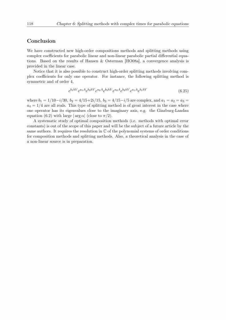
118 Chapter 6: Splitting methods with complex times for parabolic equations
Conclusion
We have constructed new high-order compositions methods and splitting methods usingcomplex coefficients for parabolic linear and non-linear parabolic partial differential equa-tions. Based on the results of Hansen & Osterman [HO08a], a convergence analysis isprovided in the linear case.
Notice that it is also possible to construct high-order splitting methods involving com-plex coefficients for only one operator. For instance, the following splitting method issymmetric and of order 4,
eb1hV ea1Aeb2hV ea2Aeb3hV ea2Aeb2hV ea1Aeb1hV (6.25)
where b1 = 1/10−i/30, b2 = 4/15+2i/15, b3 = 4/15−i/5 are complex, and a1 = a2 = a3 =a4 = 1/4 are all reals. This type of splitting method is of great interest in the case whereone operator has its eigenvalues close to the imaginary axis, e.g. the Ginzburg-Landauequation (6.2) with large | arg α| (close to π/2).
A systematic study of optimal composition methods (i.e. methods with optimal errorconstants) is out of the scope of this paper and will be the subject of a future article by thesame authors. It requires the resolution in C of the polynomial systems of order conditionsfor composition methods and splitting methods. Also, a theoretical analysis in the case ofa non-linear source is in preparation.

Appendix A
Maple script for the modified
moments of inertia
Using a symbolic manipulation package like maple, the functions in Table 3.1 can becomputed formally by comparing the Taylor series of the exact solution of (3.1), recursivelywith the series expansion of the DMV algorithm applied with modified moments of inertia.A maple script for this computation is the following:# MAPLE SCRIPT
> with(linalg): Order := 8:
# Modified moments of inertia
> s := 1+h^2*s3+h^4*s5+h^6*s7:
> d := h^2*d3+h^4*d5+h^6*d7:
> i1mod := 1/(s/i1+d): i2mod := 1/(s/i2+d): i3mod := 1/(s/i3+d):
# SERIES EXPANSION OF THE NUMERICAL SOLUTION (DMV)
> e1 := 0: e2 := 0: e3 := 0:
> for i from 1 to 13 do
> alpha := series(1+e1^2+e2^2+e3^2,h);
> e1 := series(alpha*h/2*y1/i1mod+(i2mod-i3mod)/i1mod*e2*e3,h);
> e2 := series(alpha*h/2*y2/i2mod+(i3mod-i1mod)/i2mod*e3*e1,h);
> e3 := series(alpha*h/2*y3/i3mod+(i1mod-i2mod)/i3mod*e1*e2,h);
> od:
> y1dmv := series(y1+4/h/alpha*(i2mod-i3mod)*e2*e3,h):
# Cayley transform
> Id := matrix(3,3,[1,0,0,0,1,0,0,0,1]):
> ehat := matrix(3,3,[0,-e3,e2,e3,0,-e1,-e2,e1,0]):
> Qdmv := evalm((Id+ehat)&*inverse((Id-ehat))):
# SERIES EXPANSION OF THE EXACT SOLUTION
> fncy := y1(t),y2(t),y3(t):
> fncQ := q11(t),q12(t),q13(t),q21(t),q22(t),q23(t),q31(t),q32(t),q33(t):
> Qexact := matrix(3,3,[fncQ]):
# Equations of motion
> eqy := diff(y1(t),t)=y2(t)*y3(t)*(i2-i3)/i2/i3,
> diff(y2(t),t)=y1(t)*y3(t)*(i3-i1)/i1/i3,
> diff(y3(t),t)=y1(t)*y2(t)*(i1-i2)/i2/i1:
> W := matrix(3,3,[0, -y3(t)/i3, y2(t)/i2,
> y3(t)/i3, 0, -y1(t)/i1,
> -y2(t)/i2, y1(t)/i1, 0]):
> QW := evalm(Qexact&*W):
> eqQ := seq(seq(diff(Qexact[i,j],t)=QW[i,j],j=1..3),i=1..3):
# Initial condition
> init := q11(0)=1,q12(0)=0,q13(0)=0,
> q21(0)=0,q22(0)=1,q23(0)=0,
> q31(0)=0,q32(0)=0,q33(0)=1,
> y1(0)=y1,y2(0)=y2,y3(0)=y3:
# Exact solution
> assign(dsolve(eqy,eqQ,init,fncy,fncQ,type=series)):
> y1exact := subs(t=h,y1(t)):
> Qexact := simplify(subs(t=h,matrix(3,3,[fncQ]))):
# LOCAL ERROR
> erry := simplify(series(y1exact-y1dmv,h)):
> errQ := simplify(series(Qexact[3,2]-Qdmv[3,2],h)):

120 Maple script for the modified moments of inertia
# COMPUTATION OF s3,d3,s5,d5,...
> sol := proc(coeff,err,n)
> solve(convert(series(err,h,n),polynom),coeff):
> end:
> s3 := sol(s3,erry,4): d3 := sol(d3,errQ,4):
> s5 := sol(s5,erry,6): d5 := sol(d5,errQ,6):
> s7 := sol(s7,erry,8): d7 := sol(d7,errQ,8):
# DECOMPOSITION as polynomials in H(y) and C(y)
> C:=(y1^2+y2^2+y3^2)/2: H:=(y1^2/i1+y2^2/i2+y3^2/i3)/2:
> decomp := proc(expr,vars)
> solve(subs(y1=1,y2=0,y3=0,expr),subs(y1=0,y2=1,y3=0,expr),
> subs(y1=0,y2=0,y3=1,expr),subs(y1=1,y2=1,y3=1,expr),vars);
> end:
> decomp(s3=a1*C+a2*H,a1,a2);
/ i2 i3 + i1 i3 + i1 i2 i2 + i1 + i3\
a2 = - ---------------------, a1 = ------------
\ 3 i1 i2 i3 6 i1 i2 i3 /
> decomp(s5=a1*C^2+a2*C*H+a3*H^2,a1,a2,a3);

Appendix B
Fortran code for the Preprocessed
Discrete Moser–Veselov algorithm of
order 10
SUBROUTINE DMV10 (AM,Q,POTENP,H,NSTEP,RPAR,IPAR)
C-----------------------------------------------------------------------
C PREPROCESSED DISCRETE MOSER-VESELOV ALGORITHM
C-----------------------------------------------------------------------
C PREPROCESSED DISCRETE MOSER-VESELOV ALGORITHM OF ORDER 10 FOR THE
C NUMERICAL SOLUTION OF THE EQUATIONS OF MOTION OF THE FREE RIGID BODY.
C ORTHOGONAL MATRICES ARE REPRESENTED BY QUATERNIONS.
C THE CODE IS READY TO INCLUDE AN EXERNAL POTENTIAL (SYMMETRIC STRANG
C SPLITTING OF ORDER 2).
C-----------------------------------------------------------------------
C AUTHORS: ERNST HAIRER (1) AND GILLES VILMART (1)(2)
C (1) UNIVERSITE DE GENEVE, DEPT. DE MATHEMATIQUES
C 2-4 RUE DU LIEVRE, CASE POSTALE 64
C CH-1211 GENEVE 4, SWITZERLAND
C (2) IRISA/INRIA RENNES, PROJET IPSO
C CAMPUS DE BEAULIEU, F-35042 RENNES CEDEX, FRANCE
C E-MAILS: [email protected]
C
C THIS CODE IS DESCRIBED IN:
C E. HAIRER AND G. VILMART, PREPROCESSED DISCRETE MOSER-VESELOV
C ALGORITHM FOR THE FULL DYNAMICS OF A RIGID BODY
C J. Phys. A: Math. Gen. 39 (2006) 13225-13235.
C http://stacks.iop.org/0305-4470/39/13225
C
C VERSION: AUGUST 29, 2006
C (latest correction of a small bug: December 28, 2007)
C-----------------------------------------------------------------------
C INPUT PARAMETERS
C ----------------
C AM(I) INITIAL ANGULAR MOMENTUM (I=1,2,3)
C Q(I) INITIAL QUATERNION FOR ORTHOGONAL MATRIX (I=1,2,3,4)
C H STEP SIZE
C NSTEP NUMBER OF STEPS
C POTENP NAME (EXTERNAL) OF SUBROUTINE FOR AN EXTERNAL POTENTIAL
C SUBROUTINE POTENP(Q,POTP,RPAR,IPAR)
C DIMENSION Q(4),POTP(3)
C POTP(1)=... ETC.
C RPAR,IPAR REAL AND INTEGER PARAMETERS (OR PARAMETER ARRAYS) WHICH
C CAN BE USED FOR COMMUNICATION BETWEEN SUBROUTINES
C RPAR(11), RPAR(12), RPAR(13) ARE THE THREE MOMENTS OF INERTIA OF
C THE RIGID BODY
C
C OUTPUT PARAMETERS
C -----------------

122 Fortran code for the Preprocessed Discrete Moser–Veselov algorithm of order 10
C AM(I) SOLUTION (ANGULAR MOMENTUM) AT ENDPOINT
C Q(I) SOLUTION (QUATERNION) AT ENDPOINT
C-----------------------------------------------------------------------
PARAMETER (MSPLIT=1)
C-----------------------------------------------------------------------
IMPLICIT REAL*8 (A-H,O-Z)
DOUBLE PRECISION Q(4),AM(3),POTP(3)
DIMENSION IPAR(20),RPAR(20)
EPS=ABS(1.D-15*H)
HA=H/2.0D0
HB=H/MSPLIT
C
HD=HB/2.0D0
HC=4.0D0/HB
AI1=RPAR(11)
AI2=RPAR(12)
AI3=RPAR(13)
C--- CONSTANT COEFFICIENTS FOR THE MODIFIED MOMENTS OF INERTIA
XI1=1.0D0/AI1+1.0D0/AI2+1.0D0/AI3
XI2=1.0D0/AI1**2+1.0D0/AI2**2+1.0D0/AI3**2
XI3=1.0D0/AI1**3+1.0D0/AI2**3+1.0D0/AI3**3
XI4=1.0D0/AI1**4+1.0D0/AI2**4+1.0D0/AI3**4
XDET=AI1*AI2*AI3
XDET2=XDET**2
XDET3=XDET**3
XDET4=XDET2**2
XS1=AI1+AI2+AI3
XS2=AI1**2+AI2**2+AI3**2
XS3=AI1**3+AI2**3+AI3**3
XS4=AI1**4+AI2**4+AI3**4
XSI=(AI1+AI2)/AI3+(AI2+AI3)/AI1+(AI3+AI1)/AI2
XSI12=(AI1+AI2)/AI3**2+(AI2+AI3)/AI1**2+(AI3+AI1)/AI2**2
XSI21=(AI1**2+AI2**2)/AI3+(AI2**2+AI3**2)/AI1+(AI3**2+AI1**2)/AI2
XSI13=(AI1+AI2)/AI3**3+(AI2+AI3)/AI1**3+(AI3+AI1)/AI2**3
XSI31=(AI1**3+AI2**3)/AI3+(AI2**3+AI3**3)/AI1+(AI3**3+AI1**3)/AI2
XSI22=(AI1**2+AI2**2)/AI3**2+(AI2**2+AI3**2)/AI1**2
& +(AI3**2+AI1**2)/AI2**2
C
S3C1=XS1/(6.0D0*XDET)
S3C2=-XI1/3.0D0
D3C1=-1.0D0/(3.0D0*XDET)
D3C2=S3C1
C
S5C1=(XS2/XDET-XI1)/(30.0D0*XDET)
S5C2=(1.0D0-XSI)/(30.0D0*XDET)
S5C3=(3.0D0*XS1/XDET+2.0D0*XI2)/60.0D0
D5C1=-XS1/XDET2/60.0D0
D5C2=XI1/XDET/10.0D0-XS2/XDET2/60.0D0
D5C3=-(9.0D0+XSI)/XDET/60.0D0
C
S7C1=(4.0D0*XDET+17.0D0*XS3-15.0D0*XDET*XSI)/(2520.0D0*XDET3)
S7C2=(9.0D0*XS1+10.0D0*XDET*XI2-6.0D0*XSI21)/(420.0D0*XDET2)
S7C3=((6.0D0*XSI12-1.0D2*XI1)*XDET+53.0D0*XS2)/(2520.0D0*XDET2)
S7C4=(15.0D0-XDET*XI3-2.0D0*XSI)/(630.0D0*XDET)
D7C1=(34.0D0*XDET*XI1-19.0D0*XS2)/(2520.0D0*XDET3)
D7C2=(XS3+2.0D0*XDET*XSI-85.0D0*XDET)/(1260.0D0*XDET3)
D7C3=(47.0D0*XS1+13.0D0*XSI21-38.0D0*XDET*XI2)/(2520.0D0*XDET2)
D7C4=(9.0D0*XDET*XI1+XDET*XSI12-11.0D0*XS2)/(1260.0D0*XDET2)
C
S9C1=(62.0D0*XS4-94.0D0*XDET*XSI21
& +66.0D0*XDET2*XI2+81.0D0*XDET*XS1)/(45360.0D0*XDET4)
S9C2=(-77.0D0*XSI31+75.0D0*XDET*XSI12
& +214.0D0*XS2-240.0D0*XDET*XI1)/(22680.0D0*XDET3)
S9C3=(26.0D0*XDET*XSI22+55.0D0*XS3+204.0D0*XDET
& -50.0D0*XDET2*XI3-59.0D0*XDET*XSI)/(7560.0D0*XDET3)
S9C4=(137.0D0*XDET*XI2-XDET*XSI13
& +3.0D0*XS1-69.0D0*XSI21)/(11340.0D0*XDET2)
S9C5=(2.0D0*XDET2*XI4+5.0D0*XDET*XSI12
& -171.0D0*XDET*XI1+159.0D0*XS2)/(45360.0D0*XDET2)
D9C1=(60.0D0*XSI*XDET-61.0D0*XS3-247.0D0*XDET)/(45360.0D0*XDET4)

Fortran code for the Preprocessed Discrete Moser–Veselov algorithm of order 10 123
D9C2=(54.0D0*XDET*XS1-XS4+218.0D0*XDET*XSI21
& -426.0D0*XDET2*XI2)/(45360.0D0*XDET4)
D9C3=(125.0D0*XDET*XI1-5.0D0*XSI31-130.0D0*XS2
& +4.0D0*XDET*XSI12)/(7560.0D0*XDET3)
D9C4=(67.0D0*XS3-735.0D0*XDET-15.0D0*XDET*XSI22
& +87.0D0*XDET*XSI+34.0D0*XDET2*XI3)/(22680.0D0*XDET3)
D9C5=(165.0D0*XS1-XDET*XSI13-9.0D0*XSI21
& -145.0D0*XDET*XI2)/(45360.0D0*XDET2)
c---
CALL POTENP(Q,POTP,RPAR,IPAR)
AM1=AM(1)-HA*POTP(1)
AM2=AM(2)-HA*POTP(2)
AM3=AM(3)-HA*POTP(3)
c
DO ISTEP=1,NSTEP
C --- COMPUTATION OF THE MODIFIED MOMENTS OF INERTIA
HAM0=0.5D0*HB**2*(AM1**2/AI1+AM2**2/AI2+AM3**2/AI3)
ANOR0=0.5D0*HB**2*(AM1**2+AM2**2+AM3**2)
HAM2=HAM0**2
ANOR2=ANOR0**2
HAM3=HAM0**3
ANOR3=ANOR0**3
HAM4=HAM2**2
ANOR4=ANOR2**2
ANORHAM=HAM0*ANOR0
ANOR2HAM=HAM0*ANOR2
ANORHAM2=HAM2*ANOR0
ANOR3HAM=HAM0*ANOR3
ANOR2HAM2=HAM2*ANOR2
ANORHAM3=HAM3*ANOR0
CSS=1.0D0+(S3C1*ANOR0+S3C2*HAM0)
& +(S5C1*ANOR2+S5C2*ANORHAM+S5C3*HAM2)
& +(S7C1*ANOR3+S7C2*ANOR2HAM+S7C3*ANORHAM2+S7C4*HAM3)
& +(S9C1*ANOR4+S9C2*ANOR3HAM+S9C3*ANOR2HAM2
& +S9C4*ANORHAM3+S9C5*HAM4)
CDD=(D3C1*ANOR0+D3C2*HAM0)
& +(D5C1*ANOR2+D5C2*ANORHAM+D5C3*HAM2)
& +(D7C1*ANOR3+D7C2*ANOR2HAM+D7C3*ANORHAM2+D7C4*HAM3)
& +(D9C1*ANOR4+D9C2*ANOR3HAM+D9C3*ANOR2HAM2
& +D9C4*ANORHAM3+D9C5*HAM4)
AI1MODI=CSS/AI1+CDD
AI2MODI=CSS/AI2+CDD
AI3MODI=CSS/AI3+CDD
AI1MOD=1.0D0/AI1MODI
AI2MOD=1.0D0/AI2MODI
AI3MOD=1.0D0/AI3MODI
FAD1=AI2MOD-AI3MOD
FAD2=AI3MOD-AI1MOD
FAD3=AI1MOD-AI2MOD
FAC1=FAD1*AI1MODI
FAC2=FAD2*AI2MODI
FAC3=FAD3*AI3MODI
DO ISPLIT=1,MSPLIT
C --- SOLVE FOR INTERNAL STAGE
AM1I=AM1*HD*AI1MODI
AM2I=AM2*HD*AI2MODI
AM3I=AM3*HD*AI3MODI
CM1=AM1I+FAC1*AM2I*AM3I
CM2=AM2I+FAC2*CM1*AM3I
CM3=AM3I+FAC3*CM1*CM2
DO I=1,50
CM1B=CM1
CM2B=CM2
CM3B=CM3
CALPHA=1+CM1**2+CM2**2+CM3**2
CM1=CALPHA*AM1I+FAC1*CM2*CM3
CM2=CALPHA*AM2I+FAC2*CM1*CM3
CM3=CALPHA*AM3I+FAC3*CM1*CM2
ERR=ABS(CM1B-CM1)+ABS(CM2B-CM2)+ABS(CM3B-CM3)
IF (ERR.LT.EPS) GOTO 22

124 Fortran code for the Preprocessed Discrete Moser–Veselov algorithm of order 10
END DO
22 CONTINUE
C --- UPDATE Q
Q0=Q(1)
Q1=Q(2)
Q2=Q(3)
Q3=Q(4)
Q(1)=Q0-CM1*Q1-CM2*Q2-CM3*Q3
Q(2)=Q1+CM1*Q0+CM3*Q2-CM2*Q3
Q(3)=Q2+CM2*Q0+CM1*Q3-CM3*Q1
Q(4)=Q3+CM3*Q0+CM2*Q1-CM1*Q2
C --- UPDATE M
CALPHA=HC/CALPHA
AM1=AM1+FAD1*CM2*CM3*CALPHA
AM2=AM2+FAD2*CM1*CM3*CALPHA
AM3=AM3+FAD3*CM1*CM2*CALPHA
END DO
C --- PROJECTION
QUAT=1.0D0/SQRT(Q(1)**2+Q(2)**2+Q(3)**2+Q(4)**2)
Q(1)=Q(1)*QUAT
Q(2)=Q(2)*QUAT
Q(3)=Q(3)*QUAT
Q(4)=Q(4)*QUAT
C
CALL POTENP(Q,POTP,RPAR,IPAR)
AM1=AM1-H*POTP(1)
AM2=AM2-H*POTP(2)
AM3=AM3-H*POTP(3)
END DO
AM(1)=AM1+HA*POTP(1)
AM(2)=AM2+HA*POTP(2)
AM(3)=AM3+HA*POTP(3)
RETURN
END
C * * * * * * * * * * * * * * * * * * * * * * * * * * *
C --- DRIVER FOR DMV10 FOR THE MOTION OF A RIGID BODY
C * * * * * * * * * * * * * * * * * * * * * * * * * * *
include ’dmv10.f’
IMPLICIT DOUBLE PRECISION (A-H,O-Z)
DIMENSION Q(4),AM(3),RPAR(20),IPAR(20)
REAL TIME0,TIME1
EXTERNAL POTENP
C --- INITIAL VALUES
C ANGULAR MOMENTUM
AM(1)=1.8D0
AM(2)=0.4D0
AM(3)=-0.9D0
C QUATERNION
Q(1)=1.0D0
Q(2)=0.0D0
Q(3)=0.0D0
Q(4)=0.0D0
C --- MOMENTS OF INERTIA
AI1=0.6D0
AI2=0.8D0
AI3=1.0D0
RPAR(11)=AI1
RPAR(12)=AI2
RPAR(13)=AI3
C ---
H=0.01
XEND=10.0D0
NSTEP=XEND/H
H=XEND/NSTEP
WRITE (6,*) ’XEND=’,XEND,’ H=’,H,’ NSTEP=’,NSTEP
C ---
DO I=1,10
RPAR(I)=0.0D0
IPAR(I)=0

Fortran code for the Preprocessed Discrete Moser–Veselov algorithm of order 10 125
END DO
C
WRITE (6,*) ’--- INITIAL CONDITION’
WRITE (6,*) ’ AM ’,AM(1),AM(2),AM(3)
WRITE (6,*) ’ QQ ’,Q(1),Q(2),Q(3),Q(4)
CALL HAMIL(Q,AM,HAM0,RPAR,IPAR)
CALL CPU_TIME(TIME0)
C ---
CALL DMV10 (AM,Q,POTENP,H,NSTEP,RPAR,IPAR)
C ---
CALL CPU_TIME(TIME1)
CALL HAMIL(Q,AM,HAM1,RPAR,IPAR)
WRITE (6,*) ’--- SOLUTION AT ENDPOINT’
WRITE (6,*) ’ AM ’,AM(1),AM(2),AM(3)
WRITE (6,*) ’ QQ ’,Q(1),Q(2),Q(3),Q(4)
WRITE (6,*) ’ERR HAM=’,(HAM1-HAM0)/HAM0,’ TIME=’,TIME1-TIME0
STOP
END
C
SUBROUTINE HAMIL (Q,AM,HAM,RPAR,IPAR)
IMPLICIT REAL*8 (A-H,O-Z)
DIMENSION Q(4),AM(3)
DIMENSION IPAR(*),RPAR(*)
CALL POTEN(Q,POT,RPAR,IPAR)
HAM=AM(1)**2/RPAR(11)+AM(2)**2/RPAR(12)+AM(3)**2/RPAR(13)
HAM=HAM/2.0D0+POT
RETURN
END
c
SUBROUTINE POTEN(Q,POT,RPAR,IPAR)
IMPLICIT REAL*8 (A-H,O-Z)
DIMENSION Q(4)
DIMENSION IPAR(*),RPAR(*)
POT=Q(1)**2-Q(2)**2-Q(3)**2+Q(4)**2
POT=0.0D0
RETURN
END
c
SUBROUTINE POTENP(Q,POTP,RPAR,IPAR)
IMPLICIT REAL*8 (A-H,O-Z)
DIMENSION Q(4),POTP(3)
DIMENSION IPAR(*),RPAR(*)
POTP(1)=-2*(Q(1)*Q(2)+Q(3)*Q(4))
POTP(2)=-2*(Q(1)*Q(3)-Q(2)*Q(4))
POTP(1)=0.0d0
POTP(2)=0.0d0
POTP(3)=0.0d0
RETURN
END

126 Fortran code for the Preprocessed Discrete Moser–Veselov algorithm of order 10

Appendix C
Exact resolution of the two–body
Kepler problem
In several recent publications [MN02, MN04, Koz07], conservative approximations for theexact numerical resolution of the 2-body Kepler problem in R3 are proposed,
q = p, p = − K
|q|3 q, q(t0) = q0, p(t0) = p0. (C.1)
for some constant K > 0. These discretizations exactly conserve all first integrals, the an-gular momentum, the Hamiltonian and Runge-Lenz vector, and are based on the Kustaan-heimo–Stiefel transformation (1965), introduced in [KS65], which links the Kepler problemsto the four-dimensional harmonic oscillator.
However, an efficient implementation of the exact solution of the 2-body Kepler problem(C.1) using this KS transformation does not seem documented in the literature1.
Algorithm C.0.1 (Exact solution of Kepler problem (C.1), elliptic trajectory)
1. Compute the scalars
r = |q0|, P =|p0|2
2, M = qT
0 p0, A =K
r− P > 0, λ =
√2A.
2. Compute x from the implicit relation
f(x) = K arctan(x) +a1x + a2x
2 − a1x3
(1 + x2)2+ a3 = 0 (C.2)
wherea1 = r(A − P ), a2 = 2λM, a3 = −Aλh/2.
This can be done with a few Newton iterations xn+1 = xn − f(xn)/f ′(xn).
3. The solution of (C.1) at time t = t0 +h is given by updating q0 and p0 (compensatedsummation can be applied, see Sect. 3.5.2):
q1 = q0 + (d1q0 + d2p0), p1 = p0 + (d3q0 + d4p0), (C.3)
1 In fact, the algorithm proposed in [Koz07] does not give the solution of the Kepler problem (C.1)after a fixed time of integration h. It gives the exact solution after a time which is not known a priori anddepends on the initial conditions.

128 Exact resolution of the 2-body Kepler problem
whered1 = −s2(1 + P/A), d2 = (csλr + s2M)/A,
d3 = −csλ(1 + P/A)/|q1|, d4 = rd1/|q1|
|q1| = r + rs2(P/A − 1) + csλM/A,
and we usec = (1 − x2)/(1 + x2) s = 2x/(1 + x2). (C.4)
Proposition C.0.2 For stepsize h smaller than half a period of elliptic motion (similarformulas hold for parabolic or hyperbolic trajectories), Algorithm C.0.1 yields the exactsolution of the 2-body Kepler problem (C.1). Also, the nonlinear equation (C.2) processesa unique solution.
Proof. Using the Kustaanheimo-Stiefel transformation (q, p) ∈ R3 × R3 7→ (Q, P ) ∈ R4 ×R4 as introduced in [KS65], the Kepler problem (C.1) can be transformed into the 4-dimensional harmonic oscillator with a transformed time t(s):
∂Q(s)
∂s=
1
4P (s)
∂P (s)
∂s= −2AQ(s)
∂t(s)
∂s= |Q(s)|2,
where we use the notations of [Koz07]. The derivation of the exact solution of this systemas a function of cos(λs), and sin(λs) is straightforward, and all formulas can be expressedin terms of (q, p) in (C.3). Then, the main idea is to put x = tan(λs0/2) where s0 isdefined implicitly by t(s0) − t0 = h. This allows to express the quantities c = cos(λs0),and s = sin(λs0) as rational functions of x (C.4), and relation t(s0) − t0 = h is equivalentto (C.2). Since the solution of t(s0)− t0 = h is unique (t(s) is an increasing function), thenon linear equation (C.2) possesses a unique solution and the algorithm is valid as long asx is well defined, i.e. λs0 < π, or equivalently the stepsize h is lower than half a period. ¤

Annexe D
Résumé de la thèse en français
Le sujet de la thèse est l’étude et la construction de méthodes numériques géométriquespour les équations différentielles, c’est-à-dire qui préservent des propriétés géométriques duflot exact, notamment la symétrie, la symplecticité des systèmes hamiltoniens, la conser-vation d’intégrales premières, la structure de Poisson, etc. Ce mémoire s’articule en troisparties étroitement liées.
Dans la première partie (Chapitres 1, 2 et 3), on introduit une nouvelle approche deconstruction d’intégrateurs numériques géométriques d’ordre élevé, en s’inspirant de lathéorie des équations différentielles modifiées (backward error analysis). Le cas des mé-thodes développables en B-séries est spécifiquement analysé, et on introduit une nouvelleloi de composition sur les B-séries. L’efficacité de cette approche est illustrée par la construc-tion d’un nouvel intégrateur géométrique d’ordre élevé pour les équations du mouvementd’un corps rigide. On obtient également une méthode numérique précise pour le calcul depoints conjugués pour les géodésiques du corps rigide.
Dans la seconde partie (Chapitre 4), on étudie dans quelle mesure les excellentes per-formances des méthodes symplectiques, pour l’intégration à long terme en astronomie eten dynamique moléculaire, persistent pour les problèmes de contrôle optimal. On discuteégalement l’extension de la théorie des équations modifiées aux problèmes de contrôle op-timal.
La dernière partie (Chapitres 5 et 6) est dédiée aux méthodes de pas fractionnaire(splitting en anglais). Dans le même esprit que les équations modifiées, on considère desméthodes de splitting pour les systèmes hamiltoniens perturbés, qui font intervenir des po-tentiels modifiés. On termine par la construction de méthodes de splitting d’ordre élevé aveccoefficients complexes pour les équations aux dérivées partielles paraboliques, notammentles problèmes de réaction-diffusion en chimie.
Chapitre 1 En s’inspirant de la théorie des équations modifiées (backward error analy-sis), on présente une nouvelle approche pour la construction d’intégrateurs géométriquesd’ordre élevé pour les équations différentielles ordinaires. On l’appelle ‘intégrateur à champsde vecteurs modifiés’, car on modifie le champ de vecteurs avant d’appliquer la méthode.Cette approche est illustrée avec la règle du point milieu appliquée à la dynamique complètedes équations du corps rigide libre. On accorde une attention particulière aux méthodesdéveloppables en B-séries pour lesquelles des formules explicites pour les équations diffé-rentielles modifiées sont données. Une nouvelle loi de composition sur les B-séries, appeléeloi de substitution, est présentée.

130 Résumé de la thèse en français
Chapitre 2 On présente la structure algébrique commune de deux lois de compositionsur les B-séries : la composition de Butcher, qui correspond à la composition du flot desintégrateurs, et la loi de substitution introduite au chapitre précédent, qui correspond àla composition de champs de vecteurs de B-séries. Les structures d’algèbre de Hopf surles arbres racinés sont un objet bien étudié, particulièrement en combinatoire, et sontcaractérisées essentiellement par une loi de coproduit. Il est bien connu que la premièreloi de composition correspond au produit de convolution sur l’algèbre de Hopf d’arbresde Connes & Kreimer pour la renormalisation en théorie des champs quantiques. Il aété démontré récemment que la loi de substitution peut être vue comme un coproduit,permettant de construire une nouvelle algèbre de Hopf d’arbres. On explique leur relationalgébrique du point de vue de l’intégration numérique géométrique.
Chapitre 3 Comme application de l’idée des intégrateurs des champs de vecteurs modi-fiés, on construit un intégrateur efficace d’ordre élevé pour les équations du mouvement ducorps rigide libre. L’algorithme “Discrete Moser-Veselov” est une discrétisation intégrabledes équations du mouvement. Il est symplectique et réversible en temps et il conserve toutesles intégrales premières du système. Son seul défaut est son faible ordre de convergence.On présente une modification de cet algorithme jusqu’à un ordre arbitrairement élevé quia un surcoût négligeable mais améliore considérablement la précision. On étudie égalementl’accumulation des erreurs d’arrondi au cours du temps et on explique comment la réduire.Enfin, on propose une modification qui permet de calculer le champ tangent, pour le calculde points conjugués sur les géodésiques de corps rigides.
Chapitre 4 Pour des problèmes de contrôle optimal, le principe du maximum de Pon-tryagin donne les conditions nécessaires d’optimalité sous la forme d’une équation différen-tielle hamiltonienne. Pour son intégration numérique, les méthodes symplectiques sont unchoix naturel. On étudie dans quelle mesure les excellentes performances des intégrateurssymplectiques pour l’intégration à long terme en astronomie et en dynamique moléculaire,s’étendent aux problèmes de contrôle optimal. Les expériences numériques et l’analyse ré-trograde montrent que, pour des problèmes en petite dimension et une trajectoire proched’une valeur critique de l’hamiltonien, les intégrateurs symplectiques ont un net avantage.On illustre cela avec les cas Martinet en géométrie sous-riemannienne. Pour des problèmescomme le transfert orbital d’un satellite ou le contrôle d’un corps rigide sous-marin, un telavantage n’est pas observé. Le système hamiltonien est un problème aux deux bouts et l’in-tervalle de temps n’est en général pas assez grand pour que les intégrateurs symplectiquespuissent bénéficier de leur préservation structurelle du flot. On discute également l’exten-sion éventuelle de la théorie de l’analyse rétrograde pour les intégrateurs symplectiques auxproblèmes de contrôle optimal.
Chapitre 5 On étudie des méthodes de splitting pour des systèmes hamiltoniens quiutilisent des potentiels modifiés contenant des crochets de Lie. On montre que cette ap-proche, initialement développée pour des équations différentielles d’ordre 2 (par exemple,problèmes à N corps en coordonnées de Jacobi), peut être aussi appliquée avec succès àdes problèmes de corps rigide asymétrique avec un potentiel externe. On illustre cela avecle corps pesant asymétrique, un modèle de satellites, et une simulation de dynamique mo-léculaire avec des sphères molles dipolaires. On construit également un nouveau processeurpour la méthode de Takahashi-Imada (une modification de Störmer-Verlet) pour atteindrel’ordre O(h10ε + h4ε2) pour des systèmes hamiltoniens perturbés, où h est le pas de tempset ε est la taille de la perturbation. Il se révèle efficace dans de nombreuses situations.

D.1 Intégration numérique géométrique 131
Chapitre 6 Le dernier chapitre est dédié aux méthodes de splitting avec coefficientscomplexes pour les équations aux dérivées partielles paraboliques linéaires et non-linéaires.Il est connu que toute méthode de splitting avec des coefficients réels d’ordre strictementplus grand que 2 possède nécessairement des coefficients négatifs. Ainsi, ces méthodes aveccoefficients réels ne peuvent pas être utilisées lorsqu’un opérateur comme le laplacien ∆n’est pas réversible en temps et ne peut pas être résolu pour des temps négatifs. Pourcontourner cette barrière d’ordre, on construit de nouvelles méthodes de splitting d’ordreélevé avec coefficients complexes, en s’appuyant sur les techniques de composition initia-lement développées pour l’intégration géométrique des équations différentielles ordinaires.On donne une justification théorique de l’ordre de convergence des méthodes introduitesdons le cas linéaire avec des opérateurs exponentiels. Nos expériences numériques montrentque l’ordre est bien celui attendu, en particulier dans le cas d’une source non-linéaire, etaussi avec la discrétisation de Peaceman-Rachford comme ingrédient de base.
D.1 Intégration numérique géométrique
Le domaine de l’intégration géométrique étant très vaste, on présente dans cette sec-tion les aspects les plus importants de l’intégration numérique géométrique des équationsdifférentielles ordinaires (voir les ouvrages [SSC94, LR04, HLW06]) pour la compréhensionde ce travail de thèse. Ces idées sont illustrées par les exemples du problème de Kepler, leproblème à trois corps en mécanique céleste, et le problème du pendule asymétrique.
Considérons un système d’équations différentielles1,
y = f(y), y(0) = y0, (D.1)
où f(y) est un champ de vecteurs suffisamment différentiable. La première et la plus simpledes méthodes numériques est due à Euler [Eul68] en 1768,
yn+1 = yn + hf(yn).
Étant donnée une longueur de pas h, on calcule récursivement des approximations y1,y2, y3, . . . des valeurs y(h), y(2h), y(3h), . . . de la solution. On l’appelle méthode d’Eulerexplicite car le calcul de yn+1 est effectué explicitement avec une évaluation du champ devecteurs f en supposant le vecteur yn déjà connu. A l’inverse, la méthode d’Euler implicite
yn+1 = yn + hf(yn+1)
requiert la résolution numérique d’un système non linéaire d’équations à chaque pas.
Flot exact On définit le flot (exact) ϕt de l’équation différentielle (D.1) pendant le tempst comme l’application qui, à tout point y0 de l’espace des phases associe la valeur y(t) dela solution de l’équation différentielle avec la valeur initiale y(0) = y0. Autrement dit,
ϕt(y0) = y(t) si y(0) = y0.
On appelle méthode numérique à un pas une application Φh qui approche le flot pourun temps h de l’équation différentielle (D.1).
1 Il est à noter q’un système non autonome y = f(t, y) peut être mis sous cette forme en considérantl’équation supplémentaire t = 1.
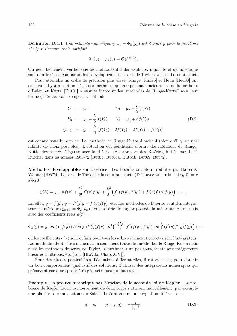
132 Résumé de la thèse en français
Définition D.1.1 Une méthode numérique yn+1 = Φh(yn) est d’ordre p pour le problème(D.1) si l’erreur locale satisfait
Φh(y) − ϕh(y) = O(hp+1).
On peut facilement vérifier que les méthodes d’Euler explicite, implicite et symplectiquesont d’ordre 1, en comparant leur développement en série de Taylor avec celui du flot exact.
Pour atteindre un ordre de précision plus élevé, Runge [Run95] et Heun [Heu00] ontconstruit il y a plus d’un siècle des méthodes qui comportent plusieurs pas de la méthoded’Euler, et Kutta [Kut01] a ensuite introduit les “méthodes de Runge-Kutta” sous leurforme générale. Par exemple, la méthode
Y1 = yn Y2 = yn +h
2f(Y1)
Y3 = yn +h
2f(Y2) Y4 = yn + hf(Y3) (D.2)
yn+1 = yn +h
6
(f(Y1) + 2f(Y2) + 2f(Y3) + f(Y4)
)
est connue sous le nom de ‘La’ méthode de Runge-Kutta d’ordre 4 (bien qu’il y ait uneinfinité de choix possibles). L’obtention des conditions d’ordre des méthodes de Runge-Kutta devint très élégante avec la théorie des arbres et des B-séries, initiée par J. C.Butcher dans les années 1963-72 [But63, But64a, But64b, But69, But72].
Méthodes développables en B-séries Les B-séries ont été introduites par Hairer &Wanner [HW74]. La série de Taylor de la solution exacte (D.1) avec valeur initiale y(0) = ys’écrit
y(h) = y + hf(y) +h2
2!f ′(y)f(y) +
h3
3!
(f ′′(f(y), f(y)) + f ′(y)f ′(y)f(y)
)+ . . .
En effet, y = f(y), y = f ′(y)y = f ′(y)f(y), etc. Les méthodes de B-séries sont des intégra-teurs numériques yn+1 = Φh(yn) dont la série de Taylor possède la même structure, maisavec des coefficients réels a(τ) :
Φh(y) = y+ha( )f(y)+h2a( )f ′(y)f(y)+h3(a( )
2f ′′(f(y), f(y))+a( )f ′(y)f ′(y)f(y)
)+. . .
où les coefficients a(τ) sont définis pour tous les arbres racinés et caractérisent l’intégrateur.Les méthodes de B-séries incluent non seulement toutes les méthodes de Runge-Kutta maisaussi les méthodes de séries de Taylor, la méthode à un pas sous-jacente aux intégrateurslinéaires multi-pas, etc (voir [HLW06, Chap.XIV]).
Pour des classes particulières d’équations différentielles, il est essentiel, pour obtenirun bon comportement qualitatif des solutions, d’utiliser des intégrateurs numériques quipréservent certaines propriétés géométriques du flot exact.
Exemple : la preuve historique par Newton de la seconde loi de Kepler Le pro-blème de Kepler décrit le mouvement de deux corps s’attirant mutuellement, par exempleune planète tournant autour du Soleil. Il s’écrit comme une équation différentielle
q = p, p = f(q) = − q
‖q‖3, (D.3)

D.1 Intégration numérique géométrique 133
où q = (q1, q2) et p = (p1, p2) représentent la position et le moment de la planète relative-ment au Soleil. Comme nous allons le voir, ce problème possède de nombreuses propriétésgéométriques, en particulier, il est hamiltonien. La seconde loi de Kepler stipule que lemoment angulaire, défini par
det(q, p) = q1p2 − q2p1
est une intégrale première, c’est-à-dire une quantité conservée le long de toute solution dusystème d’équations différentielles (D.3). Bien sûr, ce résultat peut être vérifié par simpledérivation. En 1687, Newton donna dans le ‘Theorema 1’ de son Principia [New87] uneélégante preuve géométrique de ce résultat. Étonnement, sa preuve repose sur un intégra-teur géométrique : la méthode d’Euler symplectique, qui est étroitement liée à la méthodede Störmer–Verlet, un intégrateur aujourd’hui largement utilisé en dynamique moléculairepour son excellent comportement. Dans le livre de Ostermann & Wanner [OW08], on peuttrouver une description des grandes découvertes de Newton, en fait obtenues par des rai-sonnement très géométriques.
A
B
C
V
S
e
Fig. D.1 – Reproduction du Principa de Newton (à droite)
La preuve de Newton La preuve historique s’appuie sur la discrétisation suivante de l’équa-tion différentielle (D.3)
qn+1 = qn + hpn, pn+1 = pn + hf(qn+1),
qui est connue aujourd’hui sous le nom de méthode d’Euler symplectique et peut s’inter-préter de la manière suivante. Considérons le dessin 1 de Newton, où S représente le Soleil,et soient A = qn−1, B = qn, C = qn+1, D = qn+2, etc. Pendant le premier pas de temps, laplanète se déplace de A à B en ligne droite, sans force externe, avec une vitesse constantepn−1. Au point B, une force ponctuelle f(qn) est appliquée, où la vitesse est légèrementmodifiée en direction du Soleil. Pendant le second pas de temps, le corps se déplace enC avec une vitesse constante pn et ainsi de suite. Un calcul direct montre que le schémaci-dessus implique la discrétisation naturelle suivante
qn+1 − 2qn + qn+1 = h2f(qn). (D.4)
En fait, si l’on considère (D.4) avec l’approximation de vitesse plus précise pn = (qn+1 −qn−1)/(2h), on obtient la célèbre méthode de Störmer–Verlet, ou saute-mouton (leap frogen anglais), voir plus loin une formulation à un pas équivalente.
Revenons maintenant à la preuve géométrique de Newton. La diagonale (BV ) du pa-rallélogramme ABCV est orientée vers le Soleil S car
−−→BV =
−−→BC −−−→
AB = (qn+1 − qn) − (qn − qn−1) = h2f(qn) = Const · qn.

134 Résumé de la thèse en français
On note qu’en l’absence de force, la planète aurait continué son déplacement en ligne droitede B vers e à vitesse constante, ainsi CV Be est un parallélogramme. Ensuite, les trianglesSAB et SBe ont une base de même longueur (
−−→AB =
−→Be) et la même hauteur, et donc
la même aire. De même, les triangles SBC et SBe avec la base commune SB et la mêmehauteur ont la même aire. Ainsi, les triangles SAB et SBC ont la même aire :
det(qn−1, qn − qn−1) = det(qn, qn+1 − qn).
De la même manière, tous les triangles SAB, SBC, SCD, etc, ont la même aire. En rem-plaçant pn en fonction de qn, qn+1, . . ., on obtient que le moment angulaire det(qn, pn) =det(qn−1, pn−1) est conservé exactement par la discrétisation (D.4) (aussi bien pour Eulersymplectique que pour Störmer–Verlet). On conclut que le mouvement d’un corps, soumisà une force centripède, satisfait la seconde loi de Kepler. ¤
D.1.1 Systèmes hamiltoniens et intégrateurs symplectiques
Une des classes de problèmes les plus importantes en intégration numérique géométriqueest la classe des systèmes hamiltoniens, voir l’article introductif [Hai05]. Il s’agit d’équationsdifférentielles de la forme
p = −Hq(p, q), q = Hp(p, q)
où H(p, q) est une fonction scalaire représentant l’énergie totale du système, les vecteurs qet p de dimension d représentent la position et le moment, et d est le nombre de degrés deliberté. Ici, Hp et Hq sont les vecteurs des dérivées partielles. Le système peut se réécrirematriciellement sous la forme (D.1)
y = J−1∇H(y) avec J =
(0 Id
−Id 0
), (D.5)
où le vecteur y = (p, q)T est de dimension 2d dans l’espace des phases, et Id est la matriceidentité de taille d. Par exemple, le problème de Kepler (D.3) est un système hamiltonienà d = 2 degrés de liberté, avec H(p, q) = pT p/2 + 1/‖q‖.
Les systèmes hamiltoniens possèdent les deux propriétés fondamentales suivantes :
Conservation de l’énergie L’énergie H(y) = H(p, q) est constante le long de toute so-lution de l’équation différentielle. On dit que c’est une intégrale première du système.On peut le montrer facilement par dérivation : d
dtH(y(t)) = 0.
Symplecticité La matrice jacobienne du flot ϕt des dérivées par rapport à y du systèmehamiltonien (D.5) vérifie l’identité matricielle (Poincaré [Poi92])
ϕ′t(y)T Jϕ′
t(y) = J.
En fait, cette propriété caractérise les systèmes hamiltoniens [HLW06, TheoremVI.2.8]. Elle implique la préservation du volume (|detΦ′
h(y)| = 1) et est équivalenten dimension d = 1, voir [HLW06, Sect. VI.2].
Ceci motive la définition suivante :
Définition D.1.2 Un intégrateur numérique yn+1 = Φh(yn) est symplectique pour un sys-tème hamiltonien (D.5) si la matrice jacobienne du flot numérique satisfait
Φ′h(y)T JΦ′
h(y) = J
pour tout pas de temps h (suffisamment petit).

D.1 Intégration numérique géométrique 135
Malheureusement, un intégrateur numérique ne peut pas être simultanément symplectiqueet préserver l’énergie exactement, sinon il se réduit à une transformation du temps du flotexact. Ce résultat est dû à Ge & Marsden [GM88] et une preuve algébrique est donnée parChartier, Faou & Murua [CFM06]. Cependant, un intégrateur symplectique conserve pardéfinition d(2d − 1) invariants, et nous verrons par la suite que sous certaines hypothèses,il préserve bien l’énergie des systèmes hamiltoniens sur des temps exponentiellement longs.
On commence par quelques exemples de méthodes symplectiques.
La règle du point milieu Un des intégrateurs symplectiques les plus simples est larègle du point milieu
yn+1 = yn + hf(yn + yn+1
2
).
C’est une méthode de Runge-Kutta à deux étages et donc une méthode de B-séries.Les deux intégrateurs suivants ne sont pas des méthodes de B-séries mais de P-séries,
une extension naturelle aux systèmes partitionnés, faisant intervenir des arbres bicolores.
Méthode d’Euler symplectique En combinant les méthodes d’Euler explicite et im-plicite, on obtient deux méthodes adjointes (désignées sous le même nom),
pn+1 = pn − hHq(pn+1, qn)qn+1 = qn + hHp(pn+1, qn)
et
pn+1 = pn − hHq(pn, qn+1)qn+1 = qn + hHp(pn, qn+1)
.
Méthode de Störmer–Verlet En composant un demi-pas de chaque méthode d’Eulersymplectique, on obtient
pn+1/2 = pn − h
2Hq(pn+1/2, qn)
qn+1 = qn +h
2
(Hp(pn+1/2, qn) + Hp(pn+1/2, qn+1)
)
pn+1 = pn+1/2 −h
2Hq(pn+1/2, qn+1)
Ces méthodes apparaissent déjà dans la preuve géométrique de la seconde loi de Keplerpar Newton, présentée au début de cette introduction. Pour les hamiltoniens séparables,H(q, p) = pT p/2 + U(q) on peut montrer que cette méthode est la formulation à un pasde la discrétisation équivalente (D.4) où f(q) = −∇U(q), avec l’approximation de vitessepn = (qn+1 − qn−1)/(2h). On peut noter que les méthodes d’Euler symplectique et deStörmer–Verlet sont des schémas explicites lorsque l’hamiltonien est séparable.
Intégrateurs symétriques On peut montrer que la règle du point milieu et la méthodede Störmer–Verlet sont symétriques, c’est-à-dire
Φh Φ−h(y) = y ou de manière équivalente Φ−1−h(y) = Φh(y).
On peut le vérifier en observant que la substitution yn ↔ yn+1 et h ↔ −h ne modifie pasles formules. Ces deux intégrateurs sont donc d’ordre 2, car une méthode symétrique atoujours un ordre de convergence pair [HLW06, Theorem II.3.2].

136 Résumé de la thèse en français
J S
explicit Eulerorder 1 h = 2
225 000 steps
J S
symplectic Eulerorder 1 h = 50
9 000 steps
J
S
explicit Runge–Kuttaorder 4 h = 250
1 800 steps
J S
Störmer–Verletorder 2 h = 50
9 000 steps
Fig. D.2 – Intégrateurs symplectiques et non symplectiques pour le système Soleil-Jupiter-Saturn (grands pas de temps).
Expérience numérique : le problème à trois corps On considère le problème à troiscorps (Soleil-Jupiter-Saturne) qui est un système hamiltonien avec
H(p, q) =1
2
2∑
i=0
1
mipT
i pi − G
2∑
i=1
i−1∑
j=0
mimj
‖qi − qj‖.
On prend les conditions initiales qi(0), pi(0) dans R3, la constante G et les masses mi dans[HLW06, Table I.2.2]. À ce système, on applique la méthode d’Euler explicite avec le pasde temps h = 2 jours, la méthode d’Euler symplectique et la méthode de Störmer–Verletavec le pas bien plus grand h = 50, toutes sur une période de 450 000 jours. On donneaussi le résultat pour la méthode de Runge-Kutta explicite (D.2) d’ordre de convergence4, et donc avec une longueur de pas plus grande h = 250. Dans la figure D.2, on observeque les méthodes d’Euler symplectique et de Störmer–Verlet présentent toutes deux uncomportement correct. Pour la méthode d’Euler explicite, on observe que les planètes sontéjectées en spirales avec une énergie croissante, alors que pour la méthode Runge-Kutta(D.2) Jupiter s’écrase dans le soleil avant d’être éjectée à son tour. Il est à noter que les mé-thodes d’Euler symplectique et de Störmer–Verlet présenteraient encore un comportementcorrect avec le plus grand pas de temps h = 250.
Dans l’expérience suivante (Figure D.3), on étudie la conservation de l’énergie. Onobserve que l’erreur dans l’énergie croît linéairement avec le temps pour les méthodesnon symplectiques (Euler explicite et Runge-Kutta d’ordre 4). La justification de cettecroissance linéaire en temps est immédiate, en utilisant le fait que le flot exact ϕh conserve

D.1 Intégration numérique géométrique 137
0 1 2 3 4 5
expl
icit
Eul
erh
=2
explicit Runge–Kutta 4, h = 250
symplectic Euler, h = 50
Störmer–Verlet, h = 100
Hamiltonian error (in percents)
days (×104)
1%
0
−1%
Fig. D.3 – Conservation de l’énergie pour le système à trois corps Soleil-Jupiter-Saturn
l’hamiltonien on a
H(yn+1) − H(yn) = H(yn+1) − H(ϕh(yn)) = O(hp+1),
car yn+1 = ϕh(yn)+O(hp+1). En sommant cette estimation pour n = 0 à N −1, on obtientla borne linéaire
H(yN ) − H(y0) = O(thp),
où t = Nh et p est l’ordre de la méthode.En revanche, l’erreur dans l’énergie reste bornée et petite pour les intégrateurs sym-
plectiques (Euler syplectique et Störmer–Verlet),
H(yN ) − H(y0) = O(hp).
L’explication théorique de ce comportement est due à Benettin & Giorgilli [BG94] et Tang[Tan94], voir [HLW06, Sect. IX.8]. Elle s’obtient en utilisant la théorie de l’analyse rétro-grade (backward error analysis).
D.1.2 L’analyse rétrograde
Considérons un système d’équations différentielles ordinaires (D.1) y = f(y), et unintégrateur numérique
yn+1 = Φh(yn).
L’idée de l’analyse rétrograde est de chercher et d’étudier une équation différentielle modi-fiée
z = fh(z) = f(z) + hf2(z) + h2f3(z) + . . . , z(0) = y0, (D.6)
qui soit une série formelle en puissance de la longueur de pas h, telle que la solutionnumérique yn soit formellement égale à la solution exacte de (D.6),
yn = z(nh) pour n = 0, 1, 2, . . . ,
c’est-à-dire (le dessin du haut de la Figure D.5)
Φf,h(y) = ϕfh,h
(y), (D.7)
où ϕfh,h
désigne le flot exact de (D.6).

138 Résumé de la thèse en français
L’idée de l’analyse rétrograde à été introduite par Wilkinson (1960) dans le contexte del’algèbre linéaire numérique. Elle ne fut pas appliquée à l’intégration des équations différen-tielles ordinaires avant que l’on s’intéresse au comportement en temps longs des solutionsnumériques. Ruth [Rut83] utilisa l’idée de l’analyse rétrograde pour motiver l’utilisationd’intégrateurs symplectiques pour les systèmes hamiltoniens. En fait, si on applique uneméthode symplectique à un système hamiltonien y = J−1∇H(y), l’équation différentiellemodifiée (D.6) est aussi hamiltonienne,
z = fh(z) = J−1∇H(z), H(z) = H(z) + hH2(z) + h2H3(z) + . . . .
Ceci permet de transférer des propriétés des systèmes hamiltoniens perturbés (par exemple :conservation de l’énergie, théorie KAM pour les systèmes intégrables) vers les intégrateurssymplectiques. Rapidement, il est apparu que ce type de raisonnement ne se restreint pasaux systèmes hamiltoniens mais que ces techniques s’étendent aux équations différentiellesréversibles, aux systèmes de Poisson, aux problèmes à divergence nulle, etc.
Une analyse rigoureuse à été développée dans les années quatre-vingt-dix2. On a lethéorème fondamental suivant qui justifie rigoureusement l’utilisation des méthodes sym-plectiques et qui est dû à Benettin & Giorgilli [BG94] et Tang [Tan94], voir [HLW06,Sect. IX.8].
Théoreme D.1.3 Considérons un système hamiltonien (D.5) avec H : U → R analytiqueet une méthode de B-série (ou P-série) yn+1 = Φh(yn) d’ordre p appliquée avec un pasconstant3 h. On suppose
• l’intégrateur est symplectique pour tout système hamiltonien y = J−1∇H(y) ;
• et la solution numérique reste contenue dans un compact.
Alors, pour tn = nh et h → 0 on a
H(yn) = H(y0) + O(e−γ/(ωh))
H(yn) = H(y0) + O(hp)
sur des intervalles exponentiellement longs nh ≤ eγ/(ωh), où γ > 0 dépend uniquement dela méthode et ω > 0 est relié à la constante de Lipschitz (plus haute fréquence) de l’équationdifférentielle.
Cela signifie que pour un pas h assez petit, l’énergie est bien conservée et bornée par O(hp)sur des intervalles de temps exponentiellement longs. L’idée principale de la preuve est quela solution numérique yn étant (formellement) la solution exacte du système hamiltonienperturbé via l’analyse rétrograde (D.1.2), la solution numérique conserve (formellement)exactement l’hamiltonien modifié Hh(z). Comme cet hamiltonien modifié est une petiteperturbation de taille O(hp) de l’hamiltonien original H(y), l’hamiltonien original est bienconservé.
La série formelle dans l’équation différentielle modifiée (D.6) ne converge pas en général(sauf pour des problèmes linéaires), ceci rend l’analyse rigoureuse très technique ; on estobligé de tronquer les séries de manière à ce que l’erreur soit la plus petite possible. On peutmontrer que, si l’on tronque la série (D.6) après le terme de taille O(hN(h)) où N(h) =O(1/h), on obtient l’erreur de troncature exponentiellement petite qui apparaît dans leThéorème D.1.3.
2nonante pour les Suisses3 Le comportement excellent des intégrateurs symplectiques est en général perdu avec des pas variables,
voir [HLW06, Sect. VIII.2]. Ici, on considère un pas constant h.

D.1 Intégration numérique géométrique 139
0 1 2
Hamiltonian error (in percents) h = 0.05
time (×105)
Störmer–Verlet : energy error O(h2)
simplified Takahashi-Imada method :energy error O(h2 + th4)
0.5%
−0.5%
0
−1.0%
Fig. D.4 – Erreur hamiltonienne le long de la solution numérique du pendule asymétrique.Ce contre-exemple montre que la symplecticité seule ne suffit pas pour une bonne conser-vation à long terme. Il est tiré de [HMS08].
Néanmoins, les résultats de conservation de l’énergie obtenus avec l’analyse rétrogradedécrits précédemment, ne s’appliquent PAS aux équations différentielles hautement oscil-lantes ou aux problèmes en dimension infinie (équations aux dérivées partielles), car laconclusion du Théorème D.1.3 devient caduque pour ω → ∞.
Remarque D.1.4 Il n’y a pas seulement les méthodes symplectiques qui ont un bon com-portement en temps long. Par exemple, la règle du trapèze
yn+1 = yn +h
2
(f(yn) + f(yn+1)
)
n’est pas symplectique, mais elle est conjuguée à la règle du point milieu qui, elle, estsymplectique. En effet, il existe une application χh, qui est une perturbation O(h2) del’identité, telle que
Φtraph = (χh)−1 Φpoint milieu
h χh.
Ainsi, après n pas de la méthode, on a (Φtraph )n = (χh)−1 (Φmidpoint
h )n χh et la règle dutrapèze a le même comportement en temps long que la règle du point milieu, symplectique.On appelle cela la symplecticité conjuguée ([Sto88], voir [HLW06, Sect. VI.8]).
Remark D.1.5 Il existe des résultats de conservation similaires pour les méthodes deB-séries (ou P-séries) symétriques appliquées à des systèmes intégrables réversibles (parexemple le problème de Kepler) ou des systèmes intégrables réversibles perturbés (comme leproblème à trois corps Soleil-Jupiter-Saturn), voir [HLW06, Chap.XI]. D’un point de vuepratique, la propriété de symétrie est en en général plus facile à obtenir que la symplecticitéd’un intégrateur numérique.
Pendule asymétrique Pour illustrer les difficultés que peut rencontrer une méthodesymplectique, on termine cette section par l’exemple du pendule asymétrique proposé dans[FHP04], qui est un système hamiltonien à un seul degré de liberté, avec
H(p, q) = p2/2 − cos q + 0.2 sin(2q).
On considère la condition initiale q(0) = 0, p(0) = 2.5. La vitesse initiale est suffisammentgrande pour que le pendule fasse des tours, et la vitesse reste positive au cours du temps.Ainsi, la symétrie p ↔ −p n’a pas d’influence sur la solution numérique, et la perturbation

140 Résumé de la thèse en français
q
Analyse rétrograde
y = f(y)
z = fh(z)
z(0), z(h), z(2h), . . .
=
y0, y1, y2, y3, . . .
méthodenumérique
solution
exacte
q
intégrateurs à champs de vecteurs modifiés
y = f(y)
z = fh(z)
y(0), y(h), y(2h), . . .
=
z0, z1, z2, z3, . . .
solutionexacte
méthode
numérique
Fig. D.5 – L’analyse rétrograde comparée aux intégrateurs à champs de vecteurs modifiés
+0.2 sin(2q) dans l’hamiltonien détruit la symétrie q ↔ −q. La Remarque D.1.5 pourles méthodes symétriques ne s’applique donc pas pour ce problème. Pour la méthode deStörmer–Verlet (voir Figure D.4 avec le pas h = 0.05), l’énergie est bien conservée au coursdu temps, et c’est une conséquence directe du Théorème D.1.3. On pourrait opposer que lasolution ne reste pas contenue dans un compact, car q(t) croit indéfiniment pendant que lependule fait des tours. Néanmoins, l’angle du pendule est en fait défini modulo 2π, ainsi,l’espace des phases naturel pour (p, q) est le cylindre R × [0, 2π], et la solution est en faitpériodique.
A l’inverse, pour la méthode de Takahashi-Imada simplifiée, l’énergie n’est pas bienconservée, et on observe un biais linéaire dans la Figure D.4 (même pas de temps h = 0.05).Cette méthode possède le même ordre de convergence 2 que Störmer–Verlet. Il s’agit d’unemodification où le champs f(q) est remplacé par f(q + h2/12 f(q)) dans la définition. Lamotivation pour cela est que la nouvelle méthode est d’ordre effectif 4, c’est-à-dire qu’ilexiste un changement de coordonnées χh tel que χ−1
h Φh χh est d’ordre 4. Le conceptd’ordre effectif a été introduit initialement par Butcher [But69] dans le contexte des mé-thodes de Runge-Kutta. La méthode de Takahashi-Imada simplifiée est non symplectiqueen général (et ne vérifie donc pas les hypothèses du Théorème D.1.3), mais c’est encore uneméthode de B-série symétrique qui préserve le volume. Le flot numérique est alors sym-plectique pour le problème du pendule, car c’est un problème à un seul degré de liberté. Cecontre-exemple est tiré de [HMS08], et l’explication de la non conservation de l’énergie estque l’hamiltonien modifié n’est pas globalement défini sur le cylindre : l’intégrale sur unepériode le long de la solution exacte de la fonction coefficient H4(q, p) dans l’hamiltonienmodifié est non nulle. Ce contre-exemple simple illustre que la symplecticité seule n’est passuffisante pour assurer une bonne conservation à long terme de l’énergie.

D.2 Principaux résultats obtenus 141
D.2 Principaux résultats obtenus
On décrit ici, chapitre par chapitre, les principales idées des nouveaux résultats présen-tés dans cette thèse.
Chapitre 1 : Intégrateurs à champ de vecteurs modifié
L’analyse rétrograde est un outil théorique qui donne de nombreuses informations sur lecomportement à long terme des intégrateurs numériques géométriques. Nous allons montrerque simplement en échangeant les rôles de la “solution numérique” et de la “solution exacte”(cf. les deux schémas de la Figure D.5), on obtient un nouveau moyen de construire desintégrateurs d’ordre élevé, qui préservent les propriétés géométriques et seront utiles pourl’intégration à long terme.
Précisément, on considère comme précédemment un problème d’équation différentielleà valeur initiale (D.1) et un intégrateur numérique. Mais à présent, on cherche une équationdifférentielle modifiée z = fh(z), toujours de la forme (D.6), de sorte que la solutionnumérique zn de la méthode appliquée avec le pas h à l’équation modifiée z = fh(z)soit formellement égale à la solution exacte
Φfh,h
(y) = ϕf,h(y) (D.8)
du problème initial (D.1), c’est-à-dire
zn = y(nh) pour n = 0, 1, 2, . . . ,
(voir le schéma du bas dans la Figure D.5). Remarquons que cette équation modifiée estdifférente de celle considéré précédemment pour l’analyse rétrograde. Cependant, en raisonde sa grande similarité avec l’analyse rétrograde, tous les résultats théoriques et pratiquess’étendent dans ce nouveau contexte. L’équation différentielle modifiée est encore une sérieasymptotique en générale divergente, et ses troncatures héritent des propriétés géomé-triques du flot exact lorsqu’un intégrateur adapté est appliqué. Les fonctions coefficientsfj(z) peuvent être calculées récursivement à l’aide d’un logiciel de calcul formel commemaple. Pour cela, on développe chacun des membres de l’équation z(t + h) = Φ
fh,h(z(t))
en séries en puissances de h, et on compare les coefficients. Une fois que quelques fonctionsfj(z) sont connues, on obtient l’algorithme suivant.
Algorithme D.2.1 (intégrateurs à champ de vecteurs modifié)Considérons la troncature
z = f[r]h (z) = f(z) + hf2(z) + · · · + hr−1fr(z) (D.9)
de l’équation différentielle modifiée correspondant à l’intégrateur Φf,h(y). Alors,
zn+1 = Ψf,h(zn) := Φf[r]h
,h(zn)
définit une méthode numérique d’ordre r qui approche la solution de (D.1). On l’appelleintégrateur à champ de vecteurs modifié, car le champ de vecteurs f(y) de (D.1) est modifié
en f[r]h avant que l’intégrateur de départ soit appliqué.
Cette approche est une alternative pour construire des intégrateurs numériques d’ordreélevé. Les approches classiques sont les méthodes multi-pas, les méthode de Runge-Kutta,de séries de Taylor, l’extrapolation, la composition, et les méthodes de splitting. Elle est

142 Résumé de la thèse en français
d’un grand intérêt dans le contexte de l’intégration numérique géométrique car, comme pourl’analyse rétrograde, l’équation différentielle modifiée hérite des propriétés structurelles de(D.1) si un intégrateur adapté est appliqué.
Peu de méthodes déjà connues peuvent s’inscrire dans le cadre des intégrateurs à champde vecteurs modifié, bien que non construits de cette manière. Les plus importantes sontles méthodes de fonctions génératrices introduites par Feng [Fen86]. Ce sont des intégra-teurs symplectiques d’ordre élevé pour les systèmes hamiltoniens, obtenus en appliquantune méthode symplectique de base à un système hamiltonien modifié. L’hamiltonien cor-respondant est solution formelle d’une équation aux dérivées partielles de Hamilton-Jacobi.L’approche générale de l’algorithm D.2.1 introduite est décrite dans [CHV07b].
Chapitres 1–2 : Analyse pour les B-séries : une loi de susbstitution
La plupart des méthodes numériques a un flot développable en B-séries (notammentles méthodes de Runge–Kutta), comme introduit et étudié dans [HW74], voir [HLW06,Chap. III].
Soit T = , , , . . . l’ensemble des arbres racinés, et soit ∅ l’arbre vide. Pourτ1, . . . , τm ∈ T , on note τ = [τ1, . . . , τm] l’arbre obtenu en rattachant les racines de τ1,. . . , τm à un nouveau noeud, qui devient la racine de l’arbre τ . Les différentielles élémen-taires Ff (τ) sont définies par récurrence par
Ff ( )(y) = f(y), Ff (τ)(y) = f (m)(y)(Ff (τ1)(y), . . . , Ff (τm)(y)
). (D.10)
Étant donnés des coefficients réels a(∅) et a(τ), τ ∈ T , une B-série est une série de la forme
B(f, a) = a(∅) Id +∑
τ ∈T
h|τ |
σ(τ)a(τ)Ff (τ)
= a(∅) Id + ha( ) f + h2a( ) f ′f + h3 + h3a( ) f ′′(f, f) + . . . ,
où Id représente l’application identité Id (y) = y et les scalaires σ(τ) sont des coefficients denormalisation connus. La série de Taylor de la solution exacte de (1.1) peut s’écrire commeune B-série y(h) = B(f, e)(y0) avec des coefficients e(τ). Le flot yn+1 = Φf,h(yn) d’uneméthode de Runge-Kutta est de la forme Φf,h = B(f, a) où a(τ) dépend exclusivement descoefficients de la méthode (voir [HLW06, Chap. III] pour plus de détails).
Dans la perspective d’unifier la théorie des intégrateurs à champs de vecteurs modifiésavec l’analyse rétrograde, on définit (D.6) comme l’équation différentielle modifiée donnéepar
Φfh,h
(y) = Ψf,h(y) (D.11)
où Φ et Ψ sont deux intégrateurs numériques développables en B-séries Φf,h = B(f, a) etΨf,h = B(f, c). Pour Ψf,h(y) = ϕf,h(y) (flot exact), on retrouve la formule (D.8) pour lesintégrateurs à champs de vecteurs modifiés, tandis que pour Φ
fh,h(y) = ϕ
fh,h(y) on obtient
l’équation (D.7) pour l’analyse rétrograde.En termes de B-séries, l’équation (D.11) s’écrit B(fh, a) = B(f, c). En calculant ré-
cursivement les premiers coefficients de (1.2), on se convainc rapidement que ce sont descombinaisons linéaires de différentielles élémentaires et que fh(y) = h−1B(f, b)(y) avecdes coefficients b(τ) à déterminer (on remarque que l’on a nécessairement b(∅) = 0). Cecimotive le théorème suivant, introduit dans [CHV05].

D.2 Principaux résultats obtenus 143
Théoreme D.2.2 Pour b(∅) = 0, le champ de vecteurs h−1B(f, b) inséré dans B(·, a)donne une B-séries
B(h−1B(f, b), a
)= B(f, b ⋆ a).
On a (b ⋆ a)(∅) = a(∅), et les valeurs des premiers coefficients sont données dans la Table1.2 plus loin. Une formule générale pour (b ⋆ a)(τ) est donnée dans (1.27) en Sect. 1.4.
Éléments de la preuve. On calcule à présent à la main les coefficients de la loi de substitutionpour les premiers arbres, jusqu’à l’ordre 3. On considère une B-série
B(g, a)(y) = a(∅)y + ha( )g(y) + h2a( )g′(y)g(y) +h3
2a( )g′′(y)(g(y), g(y))
+h3a( )g′(y)g′(y)g(y) + . . . (D.12)
où le champ de vecteurs g est lui-même remplacé par une B-série g = h−1B(f, b). Endéveloppant chaque terme de la série individuellement, et en omettant l’argument (y), onobtient
hg = hb( )f + h2b( )f ′f +h3
2b( )f ′′(f, f) + h3b( )f ′f ′f + . . .
h2g′g = h2(b( )f + hb( )f ′f + ...)′(b( )f + hb( )f ′f + . . .)
= h2b( )2f ′f + 2h3b( )b( )f ′f ′f + h3b( )b( )f ′′(f, f) + . . .
h3
2g′′(g, g) =
h3
2(b( )f + . . .)′′(b( )f + . . . , b( )f + . . .)
=h3
2b( )3f ′′(f, f) + . . .
h3g′g′g = h3(b( )f + . . .)′(b( )f + . . .)′(b( )f + . . .)
= h3b( )3f ′f ′f + . . .
On substitue ensuite les expressions de hg, h2g′g, h3g′g′g, h3
2 g′′(g, g) dans (D.12), et on
regroupe les termes en hf , h2f ′f , h3f ′f ′f , h3
2 f ′′(f, f). Cela donne
B(g, a)(y) = a(∅) + ha( )b( )f + h2(a( )b( ) + a( )b( )2
)f ′f
+h3
2
(a( )b( ) + 2a( )b( )b( ) + a( )b( )3
)f ′′(f, f)
+h3(a( )b( ) + 2a( )b( )b( ) + a( )b( )3
)f ′f ′f + . . .
= B(f, b ⋆ a)(y)
On obtient ainsi les premiers coefficients de la loi de substitution :
(b ⋆ a)(∅) = a(∅)
(b ⋆ a)( ) = a( )b( )
(b ⋆ a)( ) = a( )b( ) + a( )b( )2
(b ⋆ a)( ) = a( )b( ) + 2a( )b( )b( ) + a( )b( )3
(b ⋆ a)( ) = a( )b( ) + 2a( )b( )b( ) + a( )b( )3 (D.13)

144 Résumé de la thèse en français
La détermination de l’équation modifiée définie par (D.11), c’est-à-dire des coefficientsb(τ) pour a(τ) et c(τ) donnés, dans la relation
B(h−1B(f, b), a
)= B(f, c),
revient à résoudre en b(τ) le système algébrique d’équations
(b ⋆ a)(τ) = c(τ) pour τ ∈ T. (D.14)
On remarque que
(b ⋆ a)(τ) = a( )b(τ) + · · · + a(τ)b( )|τ |,
où les trois petits points ne comportent que des arbres d’ordres strictement plus petits que|τ |. Par conséquent, pour des intégrateurs consistants Φf,h = B(f, a) et Ψf,h = B(f, c),pour lesquels a(∅) = a( ) = 1 et c(∅) = c( ) = 1, les coefficients b(τ) peuvent être calculésrécursivement à partir de (D.14). De cette manière, le calcul des champs de vecteurs fj(y)dans l’équation différentielle modifiée (D.6) ou (D.9) se réduit au calcul de coefficients réels.
Intégrateurs à champs de vecteurs modifiés. Dans ce cas, Ψf,h dans (D.11) est leh-flot exact qui est une B-série avec des coefficients e(τ). Par conséquent, les coefficientsb(τ) de l’équation différentielle modifiée pour l’intégrateur Φf,h = B(f, a) s’obtiennent àpartir de
(b ⋆ a)(τ) = e(τ) pour τ ∈ T.
Analyse rétrograde. L’équation différentielle modifiée pour une méthode Ψf,h = B(f, c)est obtenue en prenant Φf,h égal au flot exact. Ses coefficients b(τ) sont alors donnés parla relation
(b ⋆ e)(τ) = c(τ) pour τ ∈ T.
Une loi de groupe sur les B-séries Les B-séries h−1B(f, b) correspondant aux appli-cations b : T ∪ ∅ → R avec b(∅) = 0 représentent des champs de vecteurs. Le produitb ⋆ a définit une structure de groupe sur l’ensemble
c : T ∪ ∅ → R ; c(∅) = 0, c( ) = 1
représentant de tels champs de vecteurs. Son élément unité est donné par c( ) = 1 etc(τ) = 0 pour |τ | > 1, il correspond au champ de vecteurs d’origine construit à partir def(y).
Dans le chapitre 2, on étudie plus avant les propriétés algébriques de la loi de sub-stitution sur les B-séries. On présente la structure algébrique commune de deux lois decomposition sur les B-séries : la composition du groupe de Butcher, qui correspond à lacomposition du flot des intégrateurs, et la loi de substitution introduite au chapitre précé-dent qui correspond à la composition des champs de vecteurs de B-séries.
Les structures d’algèbres de Hopf sur les arbres racinés sont maintenant bien étudiées,particulièrement en combinatoire, et sont essentiellement caractérisées par une loi de co-produit. Il est bien connu que la première loi de composition correspond au produit deconvolution sur l’algèbre de Hopf d’arbres de Connes & Kreimer pour la renormalisa-tion dans la théorie des champs quantiques. Il a été démontré récemment par Calaque,Ebrahimi-Fard & Manchon [CEFM08], dans le contexte de l’algèbre combinatoire, que laloi de substitution sur les B-séries permet de définir un nouveau coproduit ∆CEM qui per-met la construction d’une nouvelle algèbre de Hopf sur les arbres, par exemple (compareravec (D.13))
∆CEM ( ) = ⊗ + 2 ⊗ + 3 ⊗

D.2 Principaux résultats obtenus 145
On montre que la nouvelle loi de substitution ainsi construite est compatible avec lacomposition standard des B-séries,
B(f, a)(B(f, b)(y)
)= B(f, b · a)(y).
Par exemple, on a la distributivité
b ⋆ (a · c) = (b ⋆ a) · (b ⋆ c).
On montre également que le sous-groupe des B-séries symplectiques (pour la compositionstandard des B-séries) est en bijection naturelle via l’analyse rétrograde avec le sous-groupedes B-séries hamiltoniennes muni de la loi de substitution.
Enfin, on explique l’extension de cette théorie aux méthodes d’intégrations partition-nées (P-séries). C’est particulièrement important dans le contexte des intégrateurs sym-plectiques.
Chapitre 3 : Un intégrateur d’ordre élevé pour le mouvement d’un corps
rigide
Pour illustrer l’efficacité que peuvent avoir les intégrateurs à champs de vecteurs mo-difiés, on considère les équations du mouvement d’un corps rigide,
y = y I−1y, Q = Q I−1y, où a =
0 −a3 a2
a3 0 −a1
−a2 a1 0
(D.15)
pour un vecteur a = (a1, a2, a3)T . Ici, I = diag(I1, I2, I3) est la matrice des moments
d’inertie, y est le vecteur du moment angulaire, et Q est la matrice orthogonale qui décritla rotation relativement à un système de coordonnées fixé. Comme intégrateur numérique,on choisit l’algorithme Discrete Moser–Veselov (DMV) [MV91],
yn+1 = Ωn yn ΩTn , Qn+1 = Qn ΩT
n , (D.16)
où la matrice orthogonale Ωn est donnée par
ΩTnD − D Ωn = h yn.
Ici, la matrice diagonale D = diag(d1, d2, d3) est déterminée par d1 + d2 = I3, d2 + d3 =I1, et d3 + d1 = I2. Cet algorithme est un excellent intégrateur géométrique et partagede nombreuses propriétés géométriques avec le flot exact. Il est symplectique, il préserveexactement l’hamiltonien, le casimir et le moment angulaire Qy (dans le référentiel fixé), etil préserve l’orthogonalité de Q. Son seul inconvénient est son faible ordre de convergencedeux.
La technique des intégrateurs à champs de vecteurs modifiés ne peut pas être appli-quée directement pour augmenter l’ordre de la méthode car l’algorithme (D.16) n’est pasdéfini pour des problèmes généraux (D.1). Il est cependant défini pour Ij arbitraires etpar conséquent on cherche des moments d’inertie modifiés Ij tels que l’algorithme DMVappliqué avec Ij donne la solution exacte de (D.15). Il est démontré dans [HV06] que celaest possible avec
1
Ij
=1
Ij
(1 + h2s3(yn) + h4s5(yn) + · · ·
)+ h2d3(yn) + h4d5(yn) + · · · . (D.17)

146 Résumé de la thèse en français
10−4 10−3
10−12
10−9
10−6
10−3
100
10−4 10−3
10−12
10−9
10−6
10−3
100error
cpu time
order 2
order 4
order 6order
8
order10
angular momentum y error
cpu time
order 2
order 4
order 6order
8
order10
rotation matrix Q
Fig. D.6 – Diagramme travail-précision pour l’intégrateur DMV (ordre 2) et les versionsmodifiées d’ordre 4, 6, 8 et 10.
Les expressions sk(y) et dk(y) peuvent être calculées avec un logiciel de calcul formel de lamême manière que l’on obtient les équations différentielles modifiées. Les premiers termessont
s3(yn) = −1
3
(1
I1+
1
I2+
1
I3
)H(yn) +
I1 + I2 + I3
6 I1 I2 I3C(yn),
d3(yn) =I1 + I2 + I3
6 I1 I2 I3H(yn) − 1
3 I1 I2 I3C(yn),
où
C(y) =1
2
(y21 + y2
2 + y23
)et H(y) =
1
2
(y21
I1+
y22
I2+
y23
I3
)
sont le casimir et l’Hamiltonien du système. L’interprétation physique de ce résultat estla suivante : après une perturbation adaptée de la forme du corps rigide, l’application del’algorithme DMV donne le mouvement exact du corps rigide de départ. En tronquant lesséries dans (D.17) après le terme h2r−2 on obtient l’algorithme DMV à champs modifiésd’ordre 2r.
Expérience numérique On considère un corps rigide asymétrique avec les momentsd’inertie I1 = 0.6, I2 = 0.8, et I3 = 1.0 sur l’intervalle [0, 10]. Les valeurs initiales sonty(0) = (1.8, 0.4,−0.9)T et Q(0) est la matrice identité. L’implémentation de l’algorithmeDMV à champs modifiés est faite à l’aide de quaternions, comme expliqué dans [HV06].Bien que H(y) et C(y) soient constants le long de la solution numérique, on recalcule lesvaleurs de Ij à chaque pas pour simuler la présence d’un potentiel externe.
On applique l’algorithme DMV et ses extensions d’ordre 4, 6, 8, et 10 avec de nombreuxpas différents, et on trace dans la Figure D.6 l’erreur globale au temps final comme unefonction du temps de calcul CPU. Les temps d’exécution sont une moyenne sur 1000expériences. Les symboles donnent les valeur obtenues avec les longueurs de pas h = 0.1et h = 0.01, respectivement.
Les figures illustrent bien les ordres de convergence espérés (l’ordre p correspond à unedroite de pente −p). Le plus intéressant est le fait qu’une grande précision est obtenue plusou moins gratuitement. Considérons les résultats obtenus avec les pas h = 0.1. L’erreurpour l’algorithme DMV (ordre 2) est supérieure à 20%. Pour un très faible surcoût, lamodification d’ordre 10 fournit une précision de plus de 11 chiffres avec le même pas detemps.

D.2 Principaux résultats obtenus 147
Points conjugués sur les géodésiques de corps rigides Dans [BF07], le lieu conjugué(l’ensemble des points conjugués) des géodésiques de corps rigides est étudié dans le cas oùdeux moments d’inertie sont égaux (par exemple I2 = I3), et le cas général asymétriqueest actuellement étudié dans [BF07].
Dans la perspective de calculer des points conjugués sur des géodésiques de corps rigides,on donne un algorithme précis pour le calcul de dérivées du flot par rapport aux conditionsinitiales. Il s’agit du champ tangent
∂y(t)
∂y0,
∂Q(t)
∂y0.
On montre que les dérivées de Q(t) peuvent être aisément approchées sous la forme
∂Qn
∂y0,j= Qnan,j , j = 1, 2, 3
où les an,j sont des matrices antisymétriques. Ensuite, les points conjugués sont simplementobtenus lorsque la matrice 3× 3 dont les colonnes sont les vecteurs an,j devient singulière.
L’idée de l’algorithme est de dériver par rapport aux conditions initiales la discrétisationd’ordre élevé des équations du mouvement données par l’algorithme DMV modifié. Onmontre que cela peut être implémenté efficacement.
Chapitre 4 : Le rôle des intégrateurs symplectiques en contrôle optimal
On considère un problème de contrôle optimal de la forme
(P )
Min Φ(x(1)),x(t) = f(x(t), u(t)), t ∈ (0, 1),x(0) = x0,
où f : Rn × Rm → Rn et Φ : Rn → R sont deux fonctions lisses (C∞), et on suppose,pour simplifier, que l’état x(t) et la fonction de contrôle u(t) sont continues. Les conditionsnécessaires d’optimalité données par le principe du maximum de Pontryagin, un outil ma-jeur en contrôle optimal (voir par exemple [Eva83, MS82]), sont les suivantes. Il existe unefonction co-état p : (0, 1) → Rn telle que la solution (P ) est solution du problème aux deuxbouts,
(OC)
x(t) = Hp(x(t), p(t), u(t))p(t) = −Hx(x(t), p(t), u(t))
H(x(t), p(t), u(t)) = minα∈A H(x(t), p(t), α)x(0) = x0, p(1) = Φ′(x(1)).
pour t ∈ (0, 1), où la fonction hamiltonienne H : Rn × Rn × Rm → R est définie par
H(x, p, u) = pT f(x, u).
De plus, l’hamiltonien est conservé, c’est-à-dire H(x(t), p(t), u(t)) est constant le long dela solution de (OC).
Le travail de [Hag00, BLV06] montre qu’appliquer une discrétisation de Runge-Kuttadirectement au problème de contrôle optimal (P ) est équivalent à appliquer une méthodede Runge-Kutta partitionnée symplectique au système hamiltonien issu de la formulationde Pontryagin du problème de contrôle optimal.

148 Résumé de la thèse en français
Par exemple, on considère la méthode d’Euler explicite avec h = 1N , et x(tk) ≈ xk, tk =
kh :
Min Φ(xN ),xk+1 = xk + hf(xk, uk), k = 0, . . . N − 1
x0 = x0.
En introduisant des multiplicateurs de Lagrange, cette discrétisation est équivalente àappliquer une méthode de Runge-Kutta partitionnée symplectique, ici la méthode d’Eulersymplectique :
xk+1 = xk + hf(xk, uk),pk+1 = pk − hpT
k+1fx(xk, uk),0 = pT
k+1fu(xk, uk), i.e uk = ϕ(xk, pk+1),
x0 = x0, pN = Φ′(xN ).
avec k = 0, . . . N − 1. Ils démontrent que ceci est vrai pour toute discrétisation de Runge-Kutta.
L’objet du Chapitre 4 est d’étudier dans quelle mesure les excellentes performances desintégrateurs symplectiques pour l’intégration à long terme en astronomie et en dynamiquemoléculaire, s’étendent aux problèmes de contrôle optimal. On étudie d’abord le cas Marti-net en géométrie sous-riemannienne. Après élimination du contrôle en utilisant le principedu maximum de Pontryagin, on aboutit à l’hamiltonien
H(q, p) =1
2
((px + pz
y2
2
)2+
p2y
(1 + βx)2
).
où q = (x, y, z)T est l’état, et p = (px, py, pz)T est l’état adjoint. La dynamique intéressante
se trouve dans l’espace à deux dimensions de coordonnées (y, py). En utilisant la théoriede l’analyse rétrograde, on montre que les intégrateurs symplectiques ont un net avantagepour le cas Martinet où β = 0 (voir Figure D.7) et aussi une perturbation non intégrable(β = −10−4) (voir Figure D.8), même si l’intégration à long terme n’est pas centrale ici.
−.5 .5
−1
1
.5
−1
1
y
pynon-symplectic meth. h = 0.05
y
pyStörmer–Verlet h = 0.05
zoom×100
Fig. D.7 – Portrait de phase dans le plan (y, py) pour le cas plan β = 0.
Néanmoins, pour des problèmes comme le transfert orbital d’un satellite ou le contrôled’un corps rigide sous-marin, un tel avantage ne peut être observé. Le système hamiltonienest un problème aux deux bouts et l’intervalle de temps n’est en général pas assez longpour que les intégrateurs symplectiques puissent bénéficier de leur préservation structurelledu flot.
L’analyse rétrograde pour des problèmes de contrôle optimal ? On discute éga-lement la possibilité d’étendre la théorie de l’analyse rétrograde et des équations modifiéesaux intégrateurs symplectiques pour le contrôle optimal. On montre que cela est possible
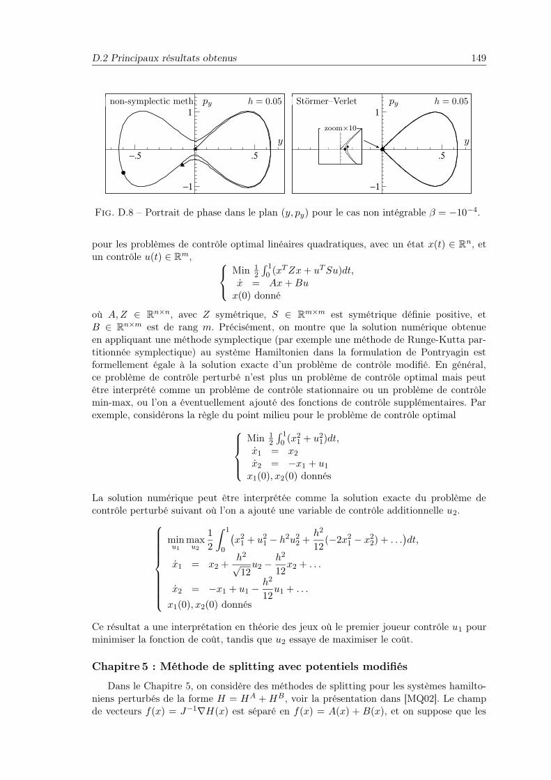
D.2 Principaux résultats obtenus 149
−.5 .5
−1
1
.5
−1
1
y
pynon-symplectic meth. h = 0.05
y
pyStörmer–Verlet h = 0.05
zoom×10
Fig. D.8 – Portrait de phase dans le plan (y, py) pour le cas non intégrable β = −10−4.
pour les problèmes de contrôle optimal linéaires quadratiques, avec un état x(t) ∈ Rn, etun contrôle u(t) ∈ Rm,
Min 12
∫ 10 (xT Zx + uT Su)dt,
x = Ax + Bux(0) donné
où A, Z ∈ Rn×n, avec Z symétrique, S ∈ Rm×m est symétrique définie positive, etB ∈ Rn×m est de rang m. Précisément, on montre que la solution numérique obtenueen appliquant une méthode symplectique (par exemple une méthode de Runge-Kutta par-titionnée symplectique) au système Hamiltonien dans la formulation de Pontryagin estformellement égale à la solution exacte d’un problème de contrôle modifié. En général,ce problème de contrôle perturbé n’est plus un problème de contrôle optimal mais peutêtre interprété comme un problème de contrôle stationnaire ou un problème de contrôlemin-max, ou l’on a éventuellement ajouté des fonctions de contrôle supplémentaires. Parexemple, considérons la règle du point milieu pour le problème de contrôle optimal
Min 12
∫ 10 (x2
1 + u21)dt,
x1 = x2
x2 = −x1 + u1
x1(0), x2(0) donnés
La solution numérique peut être interprétée comme la solution exacte du problème decontrôle perturbé suivant où l’on a ajouté une variable de contrôle additionnelle u2.
minu1
maxu2
1
2
∫ 1
0
(x2
1 + u21 − h2u2
2 +h2
12(−2x2
1 − x22) + . . .
)dt,
x1 = x2 +h2
√12
u2 −h2
12x2 + . . .
x2 = −x1 + u1 −h2
12u1 + . . .
x1(0), x2(0) donnés
Ce résultat a une interprétation en théorie des jeux où le premier joueur contrôle u1 pourminimiser la fonction de coût, tandis que u2 essaye de maximiser le coût.
Chapitre 5 : Méthode de splitting avec potentiels modifiés
Dans le Chapitre 5, on considère des méthodes de splitting pour les systèmes hamilto-niens perturbés de la forme H = HA + HB, voir la présentation dans [MQ02]. Le champde vecteurs f(x) = J−1∇H(x) est séparé en f(x) = A(x) + B(x), et on suppose que les

150 Résumé de la thèse en français
flots des champs de vecteurs A = J−1∇HA et B = J−1∇HB peuvent être approchés ef-ficacement soit exactement ou avec une grande précision. Une approche standard pour cetype de problèmes est de considérer des méthodes de splitting de la forme
eamhAebmhBeam−1hAebm−1hB · · · ea1hAeb1hB
où ehA et ehB sont les flots associés à A et B. Dans le contexte de l’intégration géométrique,ce type d’intégrateur est d’un grand intérêt, car il préserve les propriétés qualitatives dela solution exacte. En effet, lorsque A et B sont des champs de vecteurs hamiltoniens,tous les flots eaihA et ebihB sont symplectiques, et la méthode de splitting qui en résulteest symplectique en tant que composition de flots symplectiques. Ceci garantit la bonneconservation de l’énergie sur les temps longs.
Pour réduire le nombre de compositions, et donc le coût de calcul, une amélioration sub-stantielle est de considérer des méthodes avec processeur. Pour réduire le nombre d’évalua-tions à chaque pas d’intégration, l’idée des processeurs, initialement introduits par Butcher[But69] dans le contexte des méthodes de Runge-Kutta, est de considérer des compositionsde la forme
eP ehKe−P
où ehK s’appelle le noyau et doit être peu coûteux, et l’ordre de eP ehKe−P , appelé ordreeffectif, est plus grand que celui de ehK . En utilisant un pas de temps h constant, aprèsN pas, on obtient eP (ehK)Ne−P . D’abord, on applique le processeur (ou correcteur) e−P ,ensuite ehK une fois par pas, et le post-processeur eP est évalué seulement lorsque unrésultat est désiré.
Une analyse générale des méthodes de splitting symplectique avec processeur est donnéedans [BCR99].
En pratique, le principal outil pour l’obtention des contions d’ordre des méthodes desplitting est la formule de Baker-Campell-Hausdorff (BCH) (voir par exemple [HLW06,Sect. III.4.2]) qui implique que l’erreur locale pour ces méthodes est formellement unecombinaison linéaire de crochets de Lie dans l’algèbre de lie engendrée par les champs devecteurs A et B.
Maintenant, on suppose que le champs de vecteurs B est une petite perturbation duchamp de vecteurs A,
B = O(ε)
où ε est un petit paramètre. Dans ce cas, les crochets de Lie impliquant peu de B sontdominants et devraient donc être supprimés en priorité pour réduire l’erreur de la méthode.Par exemple, [A, [A, B]] = O(ε) est dominant comparé à [B, [B, A]] = O(ε2). L’idée desprocesseurs a été utilisée pour l’intégration symplectique de systèmes hamiltoniens presqueintégrables dans [WHT96, McL96].
Ces méthodes sont appelées ‘méthodes de Runge-Kutta Nyström’ dans [BCR01], carelles ont été introduites dans le cadre des équations différentielles du second ordre x =f(x). Cependant, cette classe de méthodes ne s’applique pas seulement aux équationsdifférentielles du second ordre, comme le problème à N corps avec coordonnées de Jacobiétudié dans [WH91].
La principale contribution de ce chapitre est la construction d’un nouveau processeurpour la méthode de Takahashi–Imada (une modification [Row91, TI86] du splitting deStang),
eh2B−h3
48CehAe
h2B−h3
48C .

D.2 Principaux résultats obtenus 151
pour atteindre l’ordre O(h10ε + h4ε2). On montre également que cette classe de méthodespeut être appliquée avec succès aux problèmes de corps rigide asymétrique avec un potentielexterne :
• le corps pesant asymétrique (potentiel externe linéaire) ;
• un simulation de satellite (potentiel externe quadratique) ;
• une simulation en dynamique moléculaire : c’est un problème à N corps où N moléculesd’eau sont modélisées comme des corps rigides asymétriques et interagissent commedes sphères molles magnétiques dipolaires.
Les expériences numériques montrent que cette méthode est très efficace pour ε petit,lorsque le coût d’évaluation du champ de vecteurs C = [B, [B, A]] cumulé avec avec celuide B est petit comparé au coût d’évaluation de A et B seuls.
Chapitre 6 : Méthodes de splitting avec des coefficients complexes pour
les équations paraboliques
Le dernier chapitre est dédié aux méthodes de splitting avec coefficients complexes pourles équations aux dérivées partielles paraboliques linéaires et non-linéaires. La résolutionnumérique de l’équation de la chaleur en plusieurs dimensions d’espace est maintenantbien connue mais il reste de nombreux défis en présence d’une source externe, par exemplepour les équations de réaction-diffusion, ou plus généralement pour l’équation complexede Ginzburg-Landau. D’un point de vue mathématique, ils appartiennent à la classe deséquations aux dérivées partielles semi-linéaires paraboliques et peuvent être représentéssous la forme générale
∂u
∂t= D∆u + F (u),
où chaque composante du vecteur u(x, t) ∈ Rd représente la population d’une espèce, Dest la matrice des coefficients de diffusion (souvent diagonale) et F correspond à toutesles interactions locales entre espèces. Les solutions des équations de réaction-diffusion pré-sentent un large éventail de comportements, comme les ondes voyageuses, les phénomènesd’ondes, et les solitons dissipatifs. Considérons le cas linéaire
∂u
∂t= ∆u + V u, (D.18)
où V est un opérateur linéaire, par exemple V u = v(x)u avec v(x) une fonction lisse.L’idée naturelle des méthodes de splitting consiste à combiner les exponentielles d’opé-
rateurs et∆ et etV de telle manière que l’approximation obtenue soit aussi précise quepossible. La généralisation au cas non-linéaire est immédiate en remplaçant etV par le flotde l’équation différentielle associée.
Pour un pas h > 0, l’intégrateur numérique le plus simple est la méthode de Lie-Trotter
ehV eh∆ (D.19)
qui est une approximation d’ordre 1 de la solution de (D.18), et la version symétrique
eh/2 V eh∆eh/2 V (D.20)
est connue sous le nom de splitting de Strang et est une approximation d’ordre 2. Pour desordres plus élevés, on peut considérer des méthodes de splittting de la forme
eb1hV ea1h∆eb2hV ea2h∆ . . . ebshV eash∆. (D.21)

152 Résumé de la thèse en français
Cependant, construire des méthodes d’ordre supérieur à la méthode de Strang (D.20)n’est pas aisé. Un résultat négatif montre que toute méthode de splitting (ou méthode decomposition) avec des coefficients réels d’ordre strictement plus grand que 2 possède néces-sairement un coefficient négatif à la fois pour ai et bi. Ainsi, de telles méthodes de splittingavec coefficients réels ne peuvent pas être utilisées lorsque un opérateur comme ∆ n’estpas réversible en temps et ne peut donc pas être résolu pour des temps négatifs. L’exis-tence d’au moins un coefficient négatif est montrée dans [She89, SW92], et le fait que celaconcerne les deux opérateurs est prouvée dans [GK96]. Une élégante preuve géométriqueest proposée dans [BC05].
Pour contourner cette barrière d’ordre, il y a deux possibilités. On peut utiliser unecombinaison linéaire non-convexe de produits de type (D.21), qui peuvent être obtenuspar une technique d’extrapolation [Sch02, Des01]. Une autre possibilité est de considérerdes méthodes de splitting avec des coefficients complexes de partie réelle positive. L’idéed’utiliser des coefficients complexes dans des méthodes numériques n’est pas nouvelle. Déjàen 1962/1963, Rosenbrock [Ros63] considéra des coefficients complexes pour ses méthodes.Dans [GRT02, GRT04], cette idée est exploitée pour atteindre les ordres 3 et 4 en utilisantune combinaison convexe de produit d’exponentielles avec coefficients complexes. Concer-nant les méthodes de splitting, cette liberté supplémentaire nous permet de construire desméthodes d’ordre élevé.
Il est intéressant de remarquer qu’on peut aussi augmenter l’ordre en considérant desméthodes de composition de la forme
Φγsh . . . Φγ1h (D.22)
où pour des méthodes symétriques γj = γs+1−j , et Φh est une méthode symétrique, parexemple le Strang splitting (D.20) d’ordre 2. On obtient alors la méthode de splitting
Ψh = ehγs/2 V ehγs∆eh(γs+γs−1)/2 V ehγs−1∆ . . . ehγ1∆ehγ1/2 V .
L’avantage de cette approche avec des méthodes de composition est que l’on peut remplacerla méthodes de Strang avec des exponentielles (D.20) par une discrétisation symétrique,par exemple
Φh = ΦIh/2 ΦM
h ΦEh/2
où ΦEh est le flot de la méthode d’Euler explicite yn+1 = yn + hf(yn) et ΦI
h est le flotde la méthode d’Euler implicite yn+1 = yn + hf(yn+1) pour approcher la réaction, et ΦM
h
est la discrétisation de Crank-Nicholson (équivalente à la règle du point milieu pour desproblèmes linéaires)
ΦMh =
(Id − h
2∆
)−1 (Id +
h
2∆
).
On appelle cela la formule de Peaceman-Rachford [PJ55] développée à l’origine pour l’équa-tion de la chaleur, et étendue aux problèmes de réaction-diffusion dans [DR03].
La contribution de ce chapitre est la suivante. On considère des méthodes de splittingde la forme (D.21), et on construit de nouvelles méthodes d’ordre élevé en utilisant lestechniques de composition (D.22) initialement développées pour l’intégration numériquegéométrique des équations différentielles ordinaires [HLW06]. On donne une justificationthéorique de l’ordre de convergence des méthodes introduites dans le cas linéaire pour desopérateurs exponentiels en s’appuyant sur le récent résultat de convergence de Hansen &Ostermann [HO08a]. Les principaux avantages de cette approche sont les suivants :
– la méthode de splitting hérite des propriétés de stabilité des opérateurs exponentiels ;

D.2 Principaux résultats obtenus 153
– on peut remplacer les coûteux opérateurs exponentiels par des approximations moinscoûteuses d’ordre faible sans altérer l’ordre de convergence de la méthode de splittingobtenue.
Nos simulations numériques montrent que l’ordre de convergence est celui attendu en par-ticulier dans le cas d’un terme de source non-linéaire et pour la discrétisation de Peaceman-Rachford.

154 Résumé de la thèse en français

Bibliography
[ABCK97] A. Agrachev, B. Bonnard, M. Chyba, and I. Kupka. Sub-Riemannian spherein Martinet flat case. ESAIM/COCV (Control, Optimisation and Calculus ofVariations), 2:377–448, 1997.
[BC05] S. Blanes and F. Casas. On the necessity of negative coefficients for operatorsplitting schemes of order higher than two. Appl. Num. Math., 54:23–37, 2005.
[BCF01] G. Benettin, A. M. Cherubini, and F. Fassò. A changing-chart symplecticalgorithm for rigid bodies and other Hamiltonian systems on manifolds. SIAMJ. Sci. Comput., 23:1189–1203, 2001.
[BCK99] B. Bonnard, M. Chyba, and I. Kupka. Non integrable geodesics in SR-Martinetgeometry. Proceedings of the 1997 Summer Research Institute on DifferentialGeometry and Control, University of Colorado, Boulder. - Providence R.I.,64:119–134, 1999.
[BCMR02] A. M. Bloch, P. E. Crouch, J. E. Marsden, and T. S. Ratiu. The symmetricrepresentation of the rigid body equations and their discretization. Nonlin-earity, 15:1309–1341, 2002.
[BCR99] S. Blanes, F. Casas, and J. Ros. Symplectic integrators with processing: ageneral study. SIAM J. Sci. Comput., 21:149–161, 1999.
[BCR00] S. Blanes, F. Casas, and J. Ros. Processing symplectic methods for near-integrable Hamiltonian systems. Celestial Mech. Dynam. Astronom., 77:17–35, 2000.
[BCR01] S. Blanes, F. Casas, and J. Ros. High-order Runge-Kutta-Nyström geometricmethods with processing. Appl. Num. Math., 39:245–259, 2001.
[BDL06] A. Bandrauk, E. Dehghanian, and H. Lu. Complex integration steps in de-composition of quantum exponential evolution operators. Chem. Phys. Lett.,419:346–350, 2006.
[BF07] L. Bates and F. Fassò. The conjugate locus for the Euler top. i. The axisym-metric case. International Mathematical Forum, 2(43):2109–2139, 2007.
[BG94] G. Benettin and A. Giorgilli. On the Hamiltonian interpolation of near tothe identity symplectic mappings with application to symplectic integrationalgorithms. J. Statist. Phys., 74:1117–1143, 1994.
[BH69] A. E. Bryson and Y.-C. Ho. Applied Optimal Control. Blaisdell, Waltham,MA, 1969.

156 Bibliography
[BLT99] B. Bonnard, G. Launay, and E. Trelat. The transcendence needed to computethe sphere and wave front in martinet sr-geometry. J. Math. Sci., New York,103(6):688–708, 1999.
[BLV06] J. F. Bonnans and J. Laurent-Varin. Computation of order conditions for sym-plectic partitioned Runge-Kutta schemes with application to optimal control.Numer. Math., 103(1):1–10, 2006.
[Bro37] D. Brouwer. On the accumulation of errors in numerical integration. Astro-nomical Journal, 46:149–153, 1937.
[Bro00] Ch. Brouder. Runge-Kutta methods and renormalization. Euro. Phys. J. C,12:521–534, 2000.
[Bro04] Ch. Brouder. Trees, renormalization and differential equations. BIT,44(3):425–438, 2004.
[BT01] B. Bonnard and E. Trelat. On the role of abnormal minimizers in sr-geometry.Ann. Fac. Sci. Toulouse, 6(X, 3):405–491, 2001.
[But63] J. C. Butcher. Coefficients for the study of Runge-Kutta integration processes.J. Austral. Math. Soc., 3:185–201, 1963.
[But64a] J. C. Butcher. Implicit Runge-Kutta processes. Math. Comput., 18:50–64,1964.
[But64b] J. C. Butcher. Integration processes based on Radau quadrature formulas.Math. Comput., 18:233–244, 1964.
[But69] J. C. Butcher. The effective order of Runge-Kutta methods. In J. Ll. Morris,editor, Proceedings of Conference on the Numerical Solution of DifferentialEquations, volume 109 of Lecture Notes in Math., pages 133–139, 1969.
[But72] J. C. Butcher. An algebraic theory of integration methods. Math. Comput.,26:79–106, 1972.
[CCDV08] F. Castella, P. Chartier, S. Descombes, and G. Vilmart. Splitting methodswith complex times for parabolic equations. Submitted, 2008.
[CEFM08] D. Calaque, K. Ebrahimi-Fard, and D. Manchon. Two Hopf algebras of treesinteracting. Submitted, 2008.
[CFM06] P. Chartier, E. Faou, and A. Murua. An algebraic approach to invariant pre-serving integrators: the case of quadratic and Hamiltonian invariants. Numer.Math., 103:575–590, 2006.
[CFSZ08] E. Celledoni, F. Fassò, N. Säfström, and A. Zanna. The exact computationof the free rigid body motion and its use in splitting methods. SIAM J. Sci.Comp., 30(4):2084–2112, 2008.
[CG89] M. Creutz and A. Gocksch. Higher-order hybrid Monte Carlo algorithms.Phys. Rev. Lett., 63:9–12, 1989.
[Cha03] J. E. Chambers. Symplectic integrators with complex time steps. Astron. J.,126:1119–1126, 2003.

Bibliography 157
[CHSC08a] M. Chyba, T. Haberkorn, R.N. Smith, and S.K. Choi. Autonomous under-water vehicles: Development and implementation of time and energy efficienttrajectories. Ship Technology Research, 55(2):36–48, 2008.
[CHSC08b] M. Chyba, T. Haberkorn, R.N. Smith, and S.K. Choi. Design and implemen-tation of time efficient trajectories for underwater vehicles. IEEE Journal ofOcean Engineering, 2008. (doi:10.1016/j.oceaneng.2007.07.007 ).
[CHV05] P. Chartier, E. Hairer, and G. Vilmart. A substitution law for B-series vectorfields. INRIA Report, No. 5498, 2005.
[CHV06] M. Chyba, E. Hairer, and G. Vilmart. Symplectic integrators in sub-Riemannian geometry: the Martinet case. INRIA Report, No. 6017, 2006.
[CHV07a] P. Chartier, E. Hairer, and G. Vilmart. Modified differential equations.ESAIM: Proc., 21:16–20, 2007.
[CHV07b] P. Chartier, E. Hairer, and G. Vilmart. Numerical integrators based on mod-ified differential equations. Math. Comp., 76:1941–1953, 2007.
[CHV08] M. Chyba, E. Hairer, and G. Vilmart. The role of symplectic integra-tors in optimal control. Optimal Control, Applications and Methods, 2008.(doi:10.1002/oca.855).
[CK98] A. Connes and D. Kreimer. Hopf algebras, renormalization and noncommu-tative geometry. Commun. Math. Phys., 199(1):203–242, 1998.
[CK00] A. Connes and D. Kreimer. Renormalization in quantum field theory and theRiemann–Hilbert problem. I. the Hopf algebra structure of graphs and themain theorem. Commun. Math. Phys., 210(1):249–273, 2000.
[CL98] P. Chartier and E. Lapôtre. Reversible B-series. INRIA Report, No. 1221,1998.
[CM98] A. Connes and H. Moscovici. Hopf algebras, cyclic cohomology and the trans-verse index theorem. Comm. Math. Phys., 198(1):199–246, 1998.
[CMSS94] M. P. Calvo, A. Murua, and J. M. Sanz-Serna. Modified equations for odes.Contemporary Mathematics, 172:63–74, 1994.
[Cro05] M. Crouzeix. Approximation of parabolic equations, 2005. Lecture notesavailable at http://perso.univ-rennes1.fr/michel.crouzeix/.
[CS90] P. J. Channell and J. C. Scovel. Symplectic integration of Hamiltonian sys-tems. Nonlinearity, 3:231–259, 1990.
[CS06] E. Celledoni and N. Säfström. Efficient time-symmetric simulation of torquedrigid bodies using Jacobi elliptic functions. J. Phys. A, 39:5463–5478, 2006.
[CSS94] M. P. Calvo and J. M. Sanz-Serna. Canonical B-series. Numer. Math., 67:161–175, 1994.
[Des01] S. Descombes. Convergence of a splitting method of high order for reaction-diffusion systems. Math. Comp., 70(236):1481–1501 (electronic), 2001.

158 Bibliography
[Dia96] B.O. Dia. Méthodes de directions alternées d’ordre élevé en temps. PhD thesis,Université Claude Bernard Lyon 1., 1996.
[DLM97] A. Dullweber, B. Leimkuhler, and R. McLachlan. Symplectic splitting meth-ods for rigid body molecular dynamics. J. Chem. Phys. 107 No., 15:5840–5851,1997.
[DR03] S. Descombes and M. Ribot. Convergence of the Peaceman-Rachford approx-imation for reaction-diffusion systems. Numer. Math., 95(3):503–525, 2003.
[Dür86] A. Dür. Möbius functions, incidence algebras and power series representations.In Lecture Notes in Math., volume 1202. Springer-Verlag, 1986.
[Eul68] L. Euler. Institutionum Calculi Integralis. Opera omnia, 1768.
[Eva83] L. C. Evans. An introduction to mathematical opti-mal control theory, version 0.1. Lecture notes available athttp://math.berkeley.edu/~evans/control.course.pdf, 1983.
[Fas03] F. Fassò. Comparison of splitting algorithm for the rigid body. J. Comput.Phys., 189:527–538, 2003.
[Fen86] K. Feng. Difference schemes for Hamiltonian formalism and symplectic geom-etry. J. Comp. Math., 4:279–289, 1986.
[FGS05] F. Fassò, A. Giacobbe, and N. Sansonetto. Periodic flows, rank-two Poissonstructures, and nonholonomic mechanics. Regular and Chaotic Dynamics,10(3):267–284, 2005.
[FHP04] E. Faou, E. Hairer, and T.-L. Pham. Energy conservation with non-symplecticmethods: examples and counter-examples. BIT, 44:699–709, 2004.
[For89] E. Forest. Canonical integrators as tracking codes. AIP Conference Proceed-ings, 184:1106–1136, 1989.
[FT88] S. Fauve and O. Thual. Localized structures generated by subcritical insta-bilities. J. Phys. France, 49:1829–1833, 1988.
[FWQW89] K. Feng, H. M. Wu, M.-Z. Qin, and D. L. Wang. Construction of canonicaldifference schemes for Hamiltonian formalism via generating functions. J.Comp. Math., 7:71–96, 1989.
[GB04] V. Guibout and A. Bloch. A discrete maximum principle for solving optimalcontrol problems. 43rd IEEE Conference on Decision and Control, Atlantis,Paradise Island, Bahamas, 2:1806–1811, 2004.
[GK96] D. Goldman and T. J. Kaper. nth-order operator splitting schemes and non-reversible systems. SIAM J. Numer. Anal., 33:349–367, 1996.
[GM88] Z. Ge and J. E. Marsden. Lie-Poisson Hamilton-Jacobi theory and Lie-Poissonintegrators. Phys. Lett. A, 133:134–139, 1988.
[GRT02] Z. Gegechkori, J. Rogava, and M. Tsiklauri. High degree precision decompo-sition method for the evolution problem with an operator under a split form.M2AN Math. Model. Numer. Anal., 36(4):693–704, 2002.
Bibliography 159
[GRT04] Zurab Gegechkori, Jemal Rogava, and Mikheil Tsiklauri. The fourth orderaccuracy decomposition scheme for an evolution problem. M2AN Math. Model.Numer. Anal., 38(4):707–722, 2004.
[Hag99] W. Hager. Optcon_xrk, Fortran software for solving uncon-strained control problems using explicit Runge-Kutta discretizations.http://www.math.ufl.edu/~hager/papers/optcon_xrk, 1999.
[Hag00] W. Hager. Runge-Kutta methods in optimal control and the transformedadjoint system. Numer. Math., 87(2):247–282, 2000.
[Hai94] E. Hairer. Backward analysis of numerical integrators and symplectic methods.Annals of Numerical Mathematics, 1:107–132, 1994.
[Hai99] E. Hairer. Backward error analysis for multistep methods. Numer. Math.,84:199–232, 1999.
[Hai05] E. Hairer. Long-time energy conservation of numerical integrators. Found. ofComput. Math., pages 162–180, 2005.
[Hen62] P. Henrici. Discrete Variable Methods in Ordinary Differential Equations. JohnWiley & Sons Inc., New York, 1962.
[Heu00] K. Heun. Neue Methode zur approximativen Integration der differential-gleichungen einer unabhängigen veränderlichen. Zeitschr. für Math. u. Phys.,45:23–38, 1900.
[Hig93] N. J. Higham. The accuracy of floating point summation. SIAM J. Sci.Comput., 14:783–799, 1993.
[HLW06] E. Hairer, C. Lubich, and G. Wanner. Geometric Numerical Integration.Structure-Preserving Algorithms for Ordinary Differential Equations. SpringerSeries in Computational Mathematics 31. Springer-Verlag, Berlin, second edi-tion, 2006.
[HMR08] E. Hairer, R.I. McLachlan, and A. Razakarivony. Achieving Brouwer’s lawwith implicit Runge-Kutta methods. BIT, 48:231–243, 2008.
[HMS08] E. Hairer, R. I. McLachlan, and R. D. Skeel. On energy conservation ofthe simplified Takahashi–Imada method. To appear in M2AN Math. Model.Numer. Anal., 2008.
[HO08a] E. Hansen and A. Ostermann. Exponential splitting for unbounded operators.To appear in Math. Comp., 2008.
[HO08b] E. Hansen and A. Ostermann. High order splitting methods for analytic semi-groups exist. Submitted, 2008.
[HV06] E. Hairer and G. Vilmart. Preprocessed Discrete Moser-Veselov algorithm forthe full dynamics of the rigid body. J. Phys. A, 39:13225–13235, 2006.
[HW74] E. Hairer and G. Wanner. On the Butcher group and general multi-valuemethods. Computing, 13:1–15, 1974.

160 Bibliography
[Jac50] C. G. J. Jacobi. Sur la rotation d’un corps. Journal für die reine und ange-wandte Matematik (Journal de Crelle), 39:293–350, 1850. (lu dans la séancedu 30 juillet 1849 à l’académie des sciences de Paris).
[Kah65] W. Kahan. Further remarks on reducing truncation errors. Comm. ACM,8:40, 1965.
[Kos94] P.-V. Koseleff. Formal calculus for Lie methods in Hamiltonian mechanics.PhD thesis, Lawrence Berkeley Laboratory LBID-2030, 1994. Tech. ReportUC-405, Berkeley, CA.
[Koz07] R. Kozlov. Conservative discretizations of the Kepler motion. J. Phys. A,40:4529–4539, 2007.
[KPP37] A.N. Kolmogoroff, I.G. Petrovsky, and N.S. Piscounoff. Etude de l’équationde la diffusion avec croissance de la quantité de matière et son applicationa un problème biologique. Bulletin de l’Université d’état de Moscou, SérieInternationale Section A Mathématiques et Mécanique, 1:1–25, 1937.
[KS65] P. Kustaanheimo and E. Stiefel. Perturbation theory of Kepler motion basedon spinor regularization. J. Reine Angew. Math., 218:204–19, 1965.
[Kut01] W. Kutta. Beitrag zur näherungsweisen Integration totaler Differential-gleichungen. Zeitschr. für Math. u. Phys., 46:435–453, 1901.
[LLM06] M. Leok, T. Lee, and N. H. McClamroch. Attitude maneuvers of a rigidspacecraft in a circular orbit. In Proceedings of the IEEE American ControlConference, pages 1742–1747, 2006.
[LR01] J. Laskar and P. Robutel. High order symplectic integrators for perturbedHamiltonian systems. Celest. Mech., 80:39–62, 2001.
[LR04] B. Leimkuhler and S. Reich. Simulating Hamiltonian Dynamics. CambridgeMonographs on Applied and Computational Mathematics 14. Cambridge Uni-versity Press, Cambridge, 2004.
[LS96] D. Lewis and J. C. Simo. Conserving algorithms for the n-dimensional rigidbody. Fields Inst. Commun., 10:121–139, 1996.
[McL95] R. I. McLachlan. Composition methods in the presence of small parameters.BIT, 35:258–268, 1995.
[McL96] R. I. McLachlan. More on symplectic integrators. In J. E. Marsden, G. W.Patrick, and W. F. Shadwick, editors, Integration Algorithms and ClassicalMechanics, volume 10, pages 141–149. Amer. Math. Soc., Providence, R. I.,1996.
[McL07] Robert I. McLachlan. A new implementation of symplectic Runge-Kuttamethods. SIAM J. Sci. Comput., 29(4):1637–1649, 2007.
[Mey99] K. R. Meyer. Periodic solutions of the N-body problem. In Lecture Notes inMath. 1719. Springer-Verlag, 1999.

Bibliography 161
[Mit00] J. Wm. Mitchell. A simplified variation of parameters solution for the motionof an arbitrarily torqued mass asymmetric rigid body. PhD thesis, Universityof Cincinnati, 2000.
[MKW08] H. Munthe-Kaas and W. Wright. On the Hopf algebraic structure of Lie groupintegrators. Found. Comput. Math., 8(2):227–257, 2008.
[MN02] Y. Minesaki and Y. Nakamura. A new discretization of the Kepler motionwhich conserves the Runge-Lenz vector. Phys. Lett. A, 306:127–133, 2002.
[MN04] Y. Minesaki and Y. Nakamura. A new conservative numerical integration al-gorithm for the three-dimensional Kepler motion based on the Kustaanheimo–Stiefel regularization theory. Phys. Lett. A, 324:282–92, 2004.
[Møl65] O. Møller. Quasi double-precision in floating point addition. BIT, 5:251–255,1965.
[MQ02] R. I. McLachlan and G. R. W. Quispel. Splitting methods. Acta Numerica,11:341–434, 2002.
[MS82] J. Macki and A. Strauss. Introduction to optimal control theory. Springer-Verlag, New York, 1982. Undergraduate Texts in Mathematics.
[Mur94] A. Murua. Métodos simplécticos desarrollables en P-series. PhD thesis, Univ.Valladolid, 1994.
[Mur06] A. Murua. The Hopf algebra of rooted trees, free Lie algebras, and Lie series.Found. Comput. Math., 6(4):387–426, 2006.
[MV91] J. Moser and A. P. Veselov. Discrete versions of some classical integrable sys-tems and factorization of matrix polynomials. Comm. Math. Phys., 139:217–243, 1991.
[MW01] J. E. Marsden and M. West. Discrete mechanics and variational integrators.Acta Numerica, 10:1–158, 2001.
[MZ05] R. I. McLachlan and A. Zanna. The discrete Moser–Veselov algorithm for thefree rigid body, revisited. Found. Comput. Math., 5:87–123, 2005.
[New87] I. Newton. Philosophiae Naturalis Principia Mathematica. Londini, 1687.
[OMF03] I.P. Omelyan, I.M. Mryglod, and R. Folk. Symplectic analytically integrabledecomposition algorithms: classification, derivation, and application to molec-ular dynamics, quantum and celestial mechanics simulations. Comput. Phys.Comm., 151:272–314, 2003.
[OW08] A. Ostermann and G. Wanner. Geometry by its history. Undergraduate Textsin Mathematics. Springer-Verlag, in preparation, 2008.
[PJ55] D. W. Peaceman and H. H. Rachford Jr. The numerical solution of parabolicand elliptic differential equations. J. Soc. Indust. Appl. Math., 3:28–41, 1955.
[Poi92] H. Poincaré. Les Méthodes Nouvelles de la Mécanique Céleste Tome I.Gauthier-Villars, Paris, 1892.

162 Bibliography
[Ros63] H. H. Rosenbrock. Some general implicit processes for the numerical solutionof differential equations. Comput. J., 5:329–330, 1962/1963.
[Row91] G. Rowlands. A numerical algorithm for Hamiltonian systems. J. Comput.Phys., 97:235–239, 1991.
[Run95] C. Runge. Ueber die numerische Auflösung von Differentialgleichungen. Math.Ann., 46:167–178, 1895.
[Rut83] R. D. Ruth. A canonical integration technique. IEEE Trans. Nuclear Science,NS-30:2669–2671, 1983.
[Sch02] M. Schatzman. Numerical integration of reaction-diffusion systems. Numer.Algorithms, 31(1-4):247–269, 2002. Numerical methods for ordinary differen-tial equations (Auckland, 2001).
[She89] Q. Sheng. Solving linear partial differential equations by exponential splitting.IMA J. Numer. Anal., 9:199–212, 1989.
[SSC94] J. M. Sanz-Serna and M. P. Calvo. Numerical Hamiltonian Problems. Chap-man & Hall, London, 1994.
[Sto88] D. Stoffer. On reversible and canonical integration methods. Technical ReportSAM-Report No. 88-05, ETH-Zürich, 1988.
[Suz90] M. Suzuki. Fractal decomposition of exponential operators with applicationsto many-body theories and Monte Carlo simulations. Phys. Lett. A, 146:319–323, 1990.
[SW92] G. J. Sussman and J. Wisdom. Chaotic evolution of the solar system. Science,257:56–62, 1992.
[Tan94] Y.-F. Tang. Formal energy of a symplectic scheme for Hamiltonian systemsand its applications I. Computers Math. Applic., 27:31–39, 1994.
[TI86] M. Takahashi and M. Imada. Monte Carlo calculation of quantum systems.II. Higher order correction. J. Phys. Soc. Jpn., 53:3765–3769, 1986.
[Vil08] G. Vilmart. Reducing round-off errors in rigid body dynamics. J. Comput.Phys., 227:7083–7088, 2008.
[vZS07a] R. van Zon and J. Schofield. Numerical implementation of the exact dynamicsof free rigid bodies. J. Comput. Phys., 225(1):145–164, 2007.
[vZS07b] R. van Zon and J. Schofield. Symplectic algorithms for simulations of rigidbody systems using the exact solution of free motion. Phys. Rev. E, 75:056701,2007.
[WH91] J. Wisdom and M. Holman. Symplectic maps for the n-body problem. Astron.J., 102:1528–1538, 1991.
[WHT96] J. Wisdom, M. Holman, and J. Touma. Symplectic correctors. In J. E. Mars-den, G. W. Patrick, and W. F. Shadwick, editors, Integration Algorithms andClassical Mechanics, pages 217–244. Amer. Math. Soc., Providence R. I., 1996.

Bibliography 163
[WM97] J. M. Wendlandt and J. E. Marsden. Mechanical integrators derived from adiscrete variational principle. Physica D, 106:223–246, 1997.
[Yos90] H. Yoshida. Construction of higher order symplectic integrators. Phys. Lett.A, 150:262–268, 1990.
[Zan05] A. Zanna. A note on the implicit midpoint rule and the Euler equations forthe rigid body. Private communication, 2005.

164 Bibliography

List of Figures
1 Facsimile from Newton’s Principa . . . . . . . . . . . . . . . . . . . . . . . . 52 Symplectic and non-symplectic methods for the Sun-Jupiter-Saturn system 83 Energy conservation for the three-body problem Sun-Jupiter-Saturn. . . . . 94 Hamiltonian error along the numerical solution of the asymmetric pendulum 115 Backward error analysis opposed to modifying numerical integrators . . . . 126 Work-precision diagram for the modifying DMV integrator . . . . . . . . . . 177 Phase portraits in the Martinet flat case flat case. . . . . . . . . . . . . . . 198 Phase portraits in the non-integrable perturbation of the Martinet case. . . 19
1.1 Work-precision diagram for the modifying implicit midpoint rule . . . . . . 31
3.1 Work-precision diagrams for rigid body integrators . . . . . . . . . . . . . . 583.2 Round-off errors for the Preprocessed DMV algorithm of order 10 . . . . . . 633.3 Round-off errors for the integrators based on Jacobi elliptic functions . . . . 66
4.1 Trajectories in the (x, y)-plane for the Martinet flat case . . . . . . . . . . . 754.2 Phase portraits in the (y, py)-plane for the Martinet flat case . . . . . . . . 764.3 Trajectories in the (x, y)-plane for the non integrable Martinet case . . . . . 774.4 Phase portraits in the (y, py)-plane for the non integrable Martinet case . . 774.5 Martinet flat case: asymptotic behavior of R . . . . . . . . . . . . . . . . . . 784.6 Exact solution of the orbit transfer problem . . . . . . . . . . . . . . . . . . 804.7 Satellite problem: Hamiltonian errors for various numerical integrators . . . 824.8 Submarine problem: an extrema with a conjugate point . . . . . . . . . . . 834.9 Submarine: symplectic and non-symplectic integrators for conjugate points . 84
5.1 Three body problem Sun-Jupiter-Saturn . . . . . . . . . . . . . . . . . . . . 1005.2 Asymmetric heavy top problem . . . . . . . . . . . . . . . . . . . . . . . . . 1035.3 Motion of a satellite . . . . . . . . . . . . . . . . . . . . . . . . . . . . . . . 1045.4 Molecular dynamics simulation: dipolar soft spheres . . . . . . . . . . . . . 106
6.1 Diagrams of coefficients for compositions methods . . . . . . . . . . . . . . . 1126.2 Values of maxi=1...s |argγi| for various composition methods. . . . . . . . . 1126.3 Error of composition methods for a reaction-diffusion problem . . . . . . . . 1166.4 Error of extrapolation methods for a reaction-diffusion problem . . . . . . . 117
D.1 Reproduction du Principa de Newton . . . . . . . . . . . . . . . . . . . . . 133D.2 Méthodes symplectiques ou pas pour le système Soleil-Jupiter-Saturn . . . . 136D.3 Conservation de l’énergie pour le système à trois corps Soleil-Jupiter-Saturn 137D.4 Erreur hamiltonienne pour la solution numérique du pendule asymétrique . 139D.5 L’analyse rétrograde et les intégrateurs à champs de vecteurs modifiés . . . 140D.6 Diagramme travail-précision pour l’intégrateur DMV modifié . . . . . . . . 146

166 List of Figures
D.7 Portrait de phase pour le cas Martinet plan . . . . . . . . . . . . . . . . . . 148D.8 Portrait de phase pour la perturbation non intégrable du cas Martinet . . . 149

List of Tables
1.1 Computational work and accuracy of the modifying implicit midpoint rule . 301.2 Coefficients of the substitution law for B-series vector fields . . . . . . . . . 321.3 The 8 partitions of a tree of order 4 with associated functions . . . . . . . . 351.4 The 8 partitions of a tree of order 4 with other associated functions . . . . . 36
2.1 Composition law on B-series and inverse in the Butcher group . . . . . . . . 412.2 Substitution law on B-series and corresponding coproduct . . . . . . . . . . 442.3 Inverse for the subtitution law on B-series and corresponding antipode . . . 452.4 Coefficients ω(τ) for trees of order ≤ 5. . . . . . . . . . . . . . . . . . . . . . 49
3.1 Scalar functions for the preprocessed DMV algorithm . . . . . . . . . . . . . 553.2 Geometric properties of rigid body integrators . . . . . . . . . . . . . . . . . 57
4.1 Martinet case: accuracy for the first conjugate time . . . . . . . . . . . . . . 76