Embed Size (px)
Citation preview
STUDIES OF THE MICROWAVE INSTABILITY IN THE SMALL ISOCHRONOUS RING
By
Yingjie Li
A DISSERTATION
Submitted to Michigan State University
in partial fulfillment of the requirements for the degree of
Physics—Doctor of Philosophy
2015

ABSTRACT
STUDIES OF THE MICROWAVE INSTABILITY IN THE SMALL ISOCHRONOUS RING
By
Yingjie Li
This dissertation is devoted to deepening our knowledge and understanding of the
hidden physics regarding the microwave instability of the space-charge dominated beams
in the small isochronous ring, which was observed in our previous numerical and
experimental studies.
The dissertation attempts to provide a further exploration and more accurate
description of the microwave instability by focusing on the following topics:
(a) Derivations of the full-spectrum longitudinal space charge (LSC) impedance
formula, which reflects the realistic configurations of the beam-chamber system
more closely than the existing ones.
(b) Landau damping effect. A two-dimensional (2D) dispersion relation is derived in
the dissertation, by which the microwave instability growth rates of a coasting
beam with any energy spread and emittance in the isochronous regime can be
predicted theoretically.
(c) Evolution of the beam profiles in the nonlinear regime of the microwave instability.
For this purpose, various numerical, experimental and theoretical approaches have
been employed in the research, including the simulation and measurement of the
energy spread evolution, simulated corotation of the two-macroparticle and

two-bunch models together with their comparisons with the theoretical predictions.
The simulations, experiments and theoretical predictions on the above three
topics all reach good agreements.

iv
First, I would like to dedicate this doctoral dissertation to my parents. Your eager anticipation, lasting encouragements, selfless love and dedication without reservation were crucial for me to overcome the difficulties I met both in my academic study and daily life overseas. Without your careful nurturing and inculcation from the beginning of my life, it would have been impossible for me to finish this dissertation. Second, I would like to say a Big Thank You to the following people: my elder brother, sister-in-law and cousin for their constant support, encouragement, and generous financial help, as well as taking good care of my mother and my niece.
v
ACKNOWLEDGEMENTS
My gratitude to the people who helped my graduate study at MSU is beyond words.
First of all, I would like to express my sincere thankfulness to my thesis advisor
Professor Felix Marti, who has provided great guidance on my research and trained me
from a rookie in Beam Physics to grow towards a beam scientist. I really appreciate his
patience and tolerance on my ‘slow growth rate’. His perspective insight, prudence and
strictness in the research work impressed me greatly. Without his long-term academic
supervision and support, I would not have been able to finish this dissertation. I am
particularly grateful to his constant and timely guidance even if his health condition was
sometimes not very well.
I would like to convey my special gratitude to my co-advisor, Professor Thomas
Wangler (LANL). It was a great honor for me to have had the precious opportunity to
discuss problems and receive guidance from such a world-renowned accelerator expert.
His suggestions and guidance on beam instability analysis and beam simulation are
indispensable factors for my accomplishment of the research work.
I would like to thank my committee members Professors Richard York, Michael
Syphers, Vladimir Zelevinsky, Scott Pratt, and former member Professor Jack
Baldwin for their serving in my committee. Their suggestions and guidance on my
graduate study played an important role in my academic progress.
I am greatly indebted to the following experienced researchers: Dr. Gennady
Stupakov (SLAC), Professor Alex Chao (SLAC), Dr. Lanfa Wang (SLAC), Professor S.
Y. Lee (Indiana University), Dr. K. Y. Ng (FermiLab), Dr. Fanglei Lin (JLab). Their

vi
professional suggestions and discussions were crucial for me to avoid wrong directions
and make further progress in my research; In particular, I would like to pay my special
thanks to Dr. Wang and Dr. Lin for their excellent contributions to the journal papers
collaborated between us, I did benefit and learn a lot from you on analysis methods and
paper writing skills.
I would like to give my heartfelt thanks to my colleagues Dr. Eduard Pozdeyev and
Dr. Jose Alberto Rodriguez. Dr. Pozdeyev often tailored the beam distributions for me
and taught me how to modify the input files for CYCO; Dr. Rodriguez gave me patient
explanations on the structure of SIR along with step-by-step instructions on running SIR
and tuning the beam. Their kind help was important for my research work.
Thanks a lot for the generous help and constructive suggestions on the design and test
of the SIR Energy Analyzer provided by Professor Rami Kishek, Dr. Kai Tian and Dr.
Chao Wu of University of Maryland. Also many thanks for my colleagues John Oliva,
Renan Fontus and Dr. Guillaume Machicoane of NSCL/MSU for their great work on
the design, fabrication and test of the analyzer.
Special thanks to my colleagues of NSCL Dr. Xiaoyu Wu, Dr. Yan Zhang, Dr. Qiang
Zhao, Professor Jie Wei, Professor Betty Tsang and Professor Bill Lynch for their nice
help and useful advice on my graduate study.
I am much obliged to Professors Phillip Duxbury, Wolfgang Bauer, Scott Pratt,
Michael Thoennessen, S. D. Mahanti of Department of Physics and Department
Secretary Mrs. Debbie Barratt for their excellent management and coordination work.
I am so thankful for Mr. Hersh Sisodia, the International Student Advisor at OISS.
Your useful and informative consultation was a great help for me.

vii
Thanks to the Editor Dr. William Barletta and the anonymous reviewers of Nuclear
Instruments and Methods in Physics Research A, as well as staff of publisher
Elseiver for their great job in evaluating and publishing my manuscripts.
I will never forget my friend Jack Wang for his lasting encouragement and selfless
support for my graduate study, as well as his invaluable advice on my career plan.
I would like to thank my friends Weihai Liu and his wife Dr. Cuihong Jia, Dr.
Weigang Geng, Dr. Dat Do and his wife Lisa, Mr. Dinh Pham from the bottom of my
heart for their generous financial help, encouragement for my study and concern for my
daily life.
I am very grateful to my roommate Mr. Ward Morris-Spidle and the Writing Center
of MSU for their careful proofreading, grammar corrections and polishing for my
dissertation.
I would also like to express my pure-hearted gratitude for the useful advice,
encouragement and support offered by my friends: Dr. Jianjun Luo, Dr. Wei Chang, Dr.
Chong Zhang, Dr. Liangting Sun, Dr. Yajun Guo, Dr. Xiyang Zhong, Mr. Xiaohong
Guo, Dr. Qiang Nie, Dr. Yixing Wang, Dr. Jiebing Sun, Dr. Bin Guo, Dr. Weisheng
Cao, Mrs. Huan Lian, Mrs. Li Li, Dr. Feng Shi, and Mr. Lixin Zhu.
viii
TABLE OF CONTENTS
LIST OF TABLES………………………………………………………....xi
LIST OF FIGURES……………………………………………………...xii
Chapter 1: INTRODUCTION...............…………………………………1 1.1 Brief introduction to cyclotrons………………………………………………….2 1.2 Space charge effects in isochronous cyclotrons………………………………….2
1.2.1 The incoherent transverse space charge field……………………………..3 1.2.2 The coherent radial-longitudinal space charge field………………………3 1.2.3 Vortex motion……………………………………………………………..4 1.2.4 Space charge effects and stability of short circular bunch………………..5 1.2.5 Space charge effects of long coasting bunch……………………………...5 1.2.6 Space charge effects between neighboring turns………………………….6
1.3 CYCO and Small Isochronous Ring……………………………………………..6 1.4 Summaries of previous studies of beam instability in SIR……………………..10 1.5 Major research results and conclusions in this dissertation……………………13 1.6 Brief introduction to contents of the following chapters……………………..14
Chapter 2: BASIC CONCEPTS AND BEAM DYNAMICS..........…….16 2.1 The accelerator model for the SIR……………………………………………...16 2.2 Momentum compaction factor…………………………………………………17 2.3 Dispersion function…………………………………………………………….18 2.4 Transition gamma………………………………………………………………19 2.5 Slip factor………………………………………………………………………19 2.6 Beam optics for hard-edge model of SIR………………………………………20 2.7 Negative mass instability (microwave instability)……………………………..27 2.8 Microwave instability in the isochronous regime………………………………28 2.9 Landau damping………………………………………………………………..29 2.10 Coherent and incoherent motions……………………………………………30
Chapter 3: STUDY OF LONGITUDINAL SPACE CHARGE IMP- EDANCES..…………………………………………………………….. 31
3.1 Introduction…………………………………………………………………….31 3.2 A summary of the existing LSC field models………………………………….33 3.3 Review of analytical methods for derivation of the LSC fields………………..33 3.4 LSC impedances of a rectangular beam inside a rectangular chamber and
between parallel plates………………………………………………………….34 3.4.1 Field model of a rectangular beam inside a rectangular chamber………35 3.4.2 Calculation of the space charge potentials and fields…………………….37 3.4.3 LSC impedances…………………………………………………………41

ix
3.4.4 Case studies of the LSC impedances……………………………..…….44 3.4.5 Conclusions for the rectangular beam model…….……………..………53
3.5 LSC impedances of a round beam inside a rectangular chamber and between parallel plates.……………………………………………………………...53 3.5.1 A round beam in free space………………………………………………55 3.5.2 A line charge in free space……………………………………………….55 3.5.3 A line charge between parallel plates……………………………………57 3.5.4 A line charge inside a rectangular chamber……………………………...61 3.5.5 Approximate LSC impedances of a round beam between parallel plates and inside a rectangular chamber………………………………………..62 3.5.6 Summary of some LSC impedances formulae…………………………..64
3.5.6.1 A round beam inside a round chamber………………………….64 3.5.6.2 A round beam inside a rectangular chamber in the long-
wavelength limits…………………………………………..66 3.5.6.3 A round beam between parallel plates in the long-wavelength
limits…………………………………………………………….66 3.5.7 Case study and comparisons of LSC impedances……………………….67 3.5.8 Conclusions for the model of a round beam inside rectangular chamber
(between parallel plates)…….…………………………………………..76
Chapter 4: MICROWAVE INSTABILITY AND LANDAU DAMPING EFFECTS................……………………………………………….………………78
4.1 Introduction…………………………………………………………………….78 4.2 2D dispersion relation…………………………………………………………..80
4.2.1 A brief review of the 1D growth rates formula……..…..…………..80 4.2.2 Limitations of 1D growth rates formula……..……….……………….82 4.2.3 Space-charge modified tunes and transition gammas in the isochronous
regime……………………………………………………………………85 4.2.4 2D dispersion relation……………………………………………………86
4.2.4.1 Review of the 2D dispersion relation for CSR instability of ultra-relativistic electron beams in non-isochronous regime…...87
4.2.4.2 2D dispersion relation for microwave instability of low energy beam in isochronous regime…………………………………..91
4.3 Landau damping effects in isochronous ring…………………………………...94 4.3.1 Space-charge modified coherent slip factors………………………….94 4.3.2 Exponential suppression factor………………………………………..97 4.3.3 Relations between the 1D growth rates formula and 2D dispersion
relation ……………….………………………………………………..…99 4.4 Simulation study of the microwave instability in SIR……………………….100
4.4.1 Simulated growth rates of microwave instability………………………100 4.4.2 Growth rates of instability with variable beam intensities……………..107 4.4.3 Growth rates of instability with variable beam emittance……………...108 4.4.4 Growth rates of instability with variable beam energy spread…………109 4.4.5 Possible reasons for the discrepancies between simulations and theory
in the short-wavelength limits…………………………………………..110 4.5 Conclusions……………………………………………………………………113

x
Chapter 5: DESIGN AND TEST OF ENERGY ANALYZER...............114 5.1 Introduction……………………………………………………………………114 5.2 Working principles and design considerations of the RFA……………………114 5.3 Design requirements for the SIR energy analyzer…………………………….119 5.4 A brief introduction to the UMER analyzer…………………………………...120 5.5 Design of the SIR energy analyzer……………………………………………123 5.6 Experimental test of the SIR energy analyzer………………………………...130 5.7 Conclusions……………………………………………………………………132
Chapter 6: NONLINEAR BEAM DYNAMICS OF SIR BEAM ….…133 6.1 Introduction……………………………………………………………………133 6.2 Measurement of the energy spread……………………………………………133
6.2.1 Energy spread measurement system……………………………………134 6.2.2 Data analysis of the energy spread……………………………………..137 6.2.3 Measurement results and comparisons with simulation………………..139
6.3 Corotation of cluster pair in the × field………………………………...145 6.4 Binary merging of 2D short bunches………………………………………….150 6.5 Conclusions……………………………………………………………………155
Chapter 7: CONCLUSIONS AND FUTURE WORKS….………………156 7.1 Conclusions……………………………………………………………………156 7.2 Future works…………………………………………………………………..157
APPENDICES……………………………………………………………………159 APPENDIX A : FORMALISM OF THE STANDARD TRANSFER MATRIX
FOR SIR………………………………………………………..160 APPENDIX B : TRANSFER MATRIX USED IN CHAPTER 4 AND REF.
[42]…………………………………………………………..….172
BIBLIOGRAPHY…………………………………………………………………179
xi
LIST OF TABLES
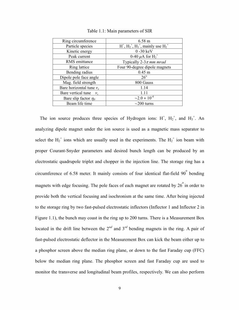
Table 1.1 Main parameters of SIR………………………..……………………………….9
Table 2.1 Parameters of SIR (hard-edge model)…………………..……………………..21
Table 5.1 Design parameters of the SIR Energy Analyzer…………..………………….119
Table 5.2 Comparisons between the UMER (2nd generation) and SIR Analyzers……...125

xii
LIST OF FIGURES
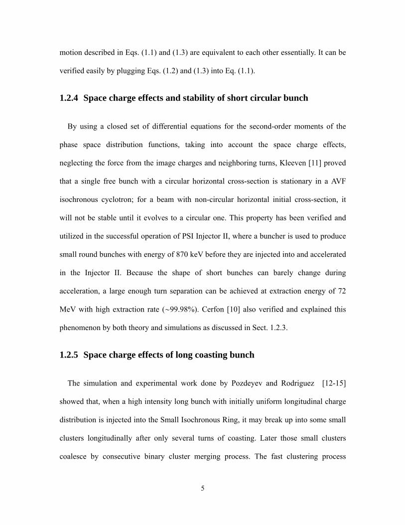
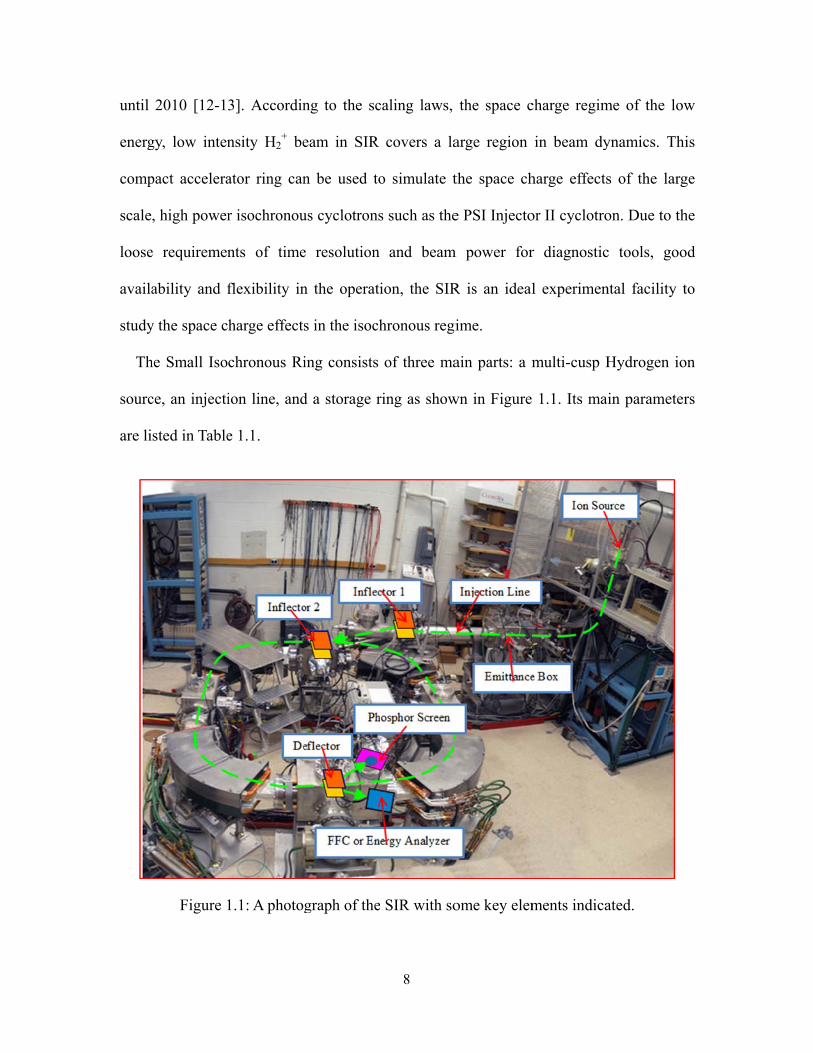
Figure 1.1 A photograph of the SIR with some key elements indicated……………….8
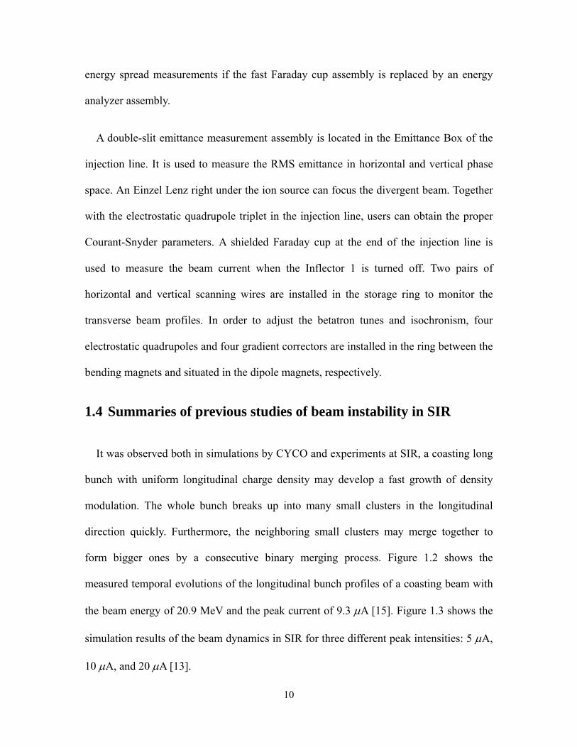
Figure 1.2 Longitudinal bunch profiles measured by the fast Faraday cup right after injection (turn 0), at turn 10 and turn 20. The current profiles measured at turn 10 and turn 20 are shifted vertically by 0.3 and 0.6, respectively [15]...11
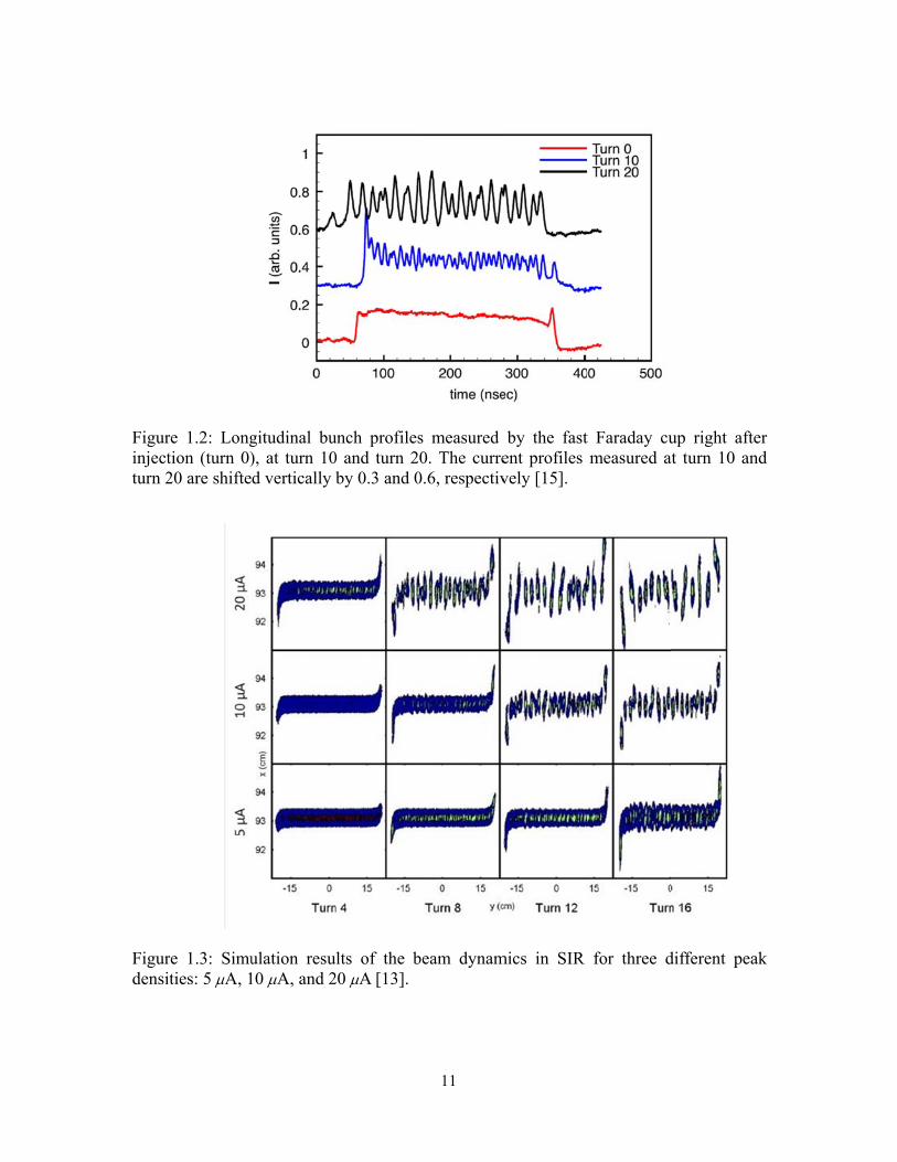
Figure 1.3 Simulation results of the beam dynamics in SIR for three different peak densities: 5 A, 10 A, and 20 A [13]………..……….…………..……….11
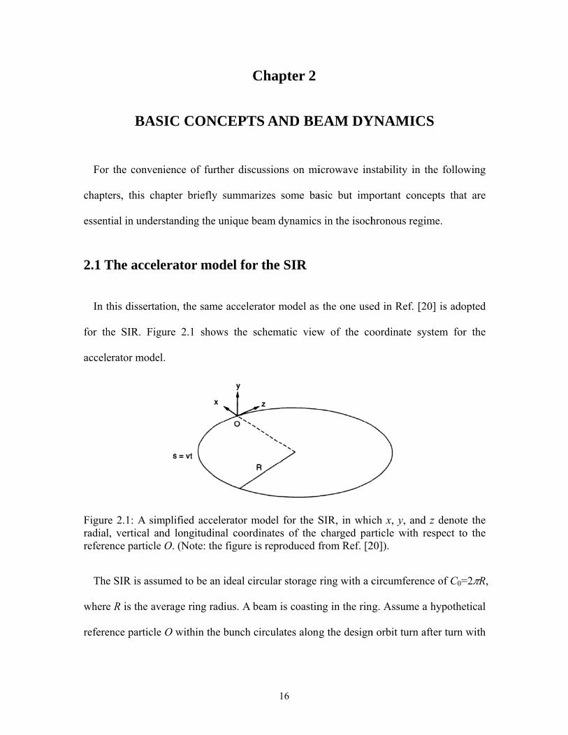
Figure 2.1 A simplified accelerator model for the SIR, in which x, y, and z denote the radial, vertical and longitudinal coordinates of the charged particle with respect to the reference particle O. (The figure is reproduced from Ref. [20])….……………………………………………………………………..16
Figure 2.2 Layout of the SIR lattice…………………………………………………....21
Figure 2.3 The optical functions v.s distance of a single period of the ring. The black rectangle schematically shows one of the dipole magnets. The legend items ‘BETX’, ‘BETY’, and ‘DX’ stand for the horizontal beta function bx(s), vertical beta function by(s), and horizontal dispersion function Dx(s), respectively. (Note: The figure is reproduced from Ref. [12])…..................22
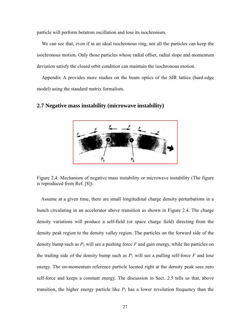
Figure 2.4 Mechanism of negative mass instability or microwave instability (The figure is reproduced from Ref. [8])……………………………………………….27
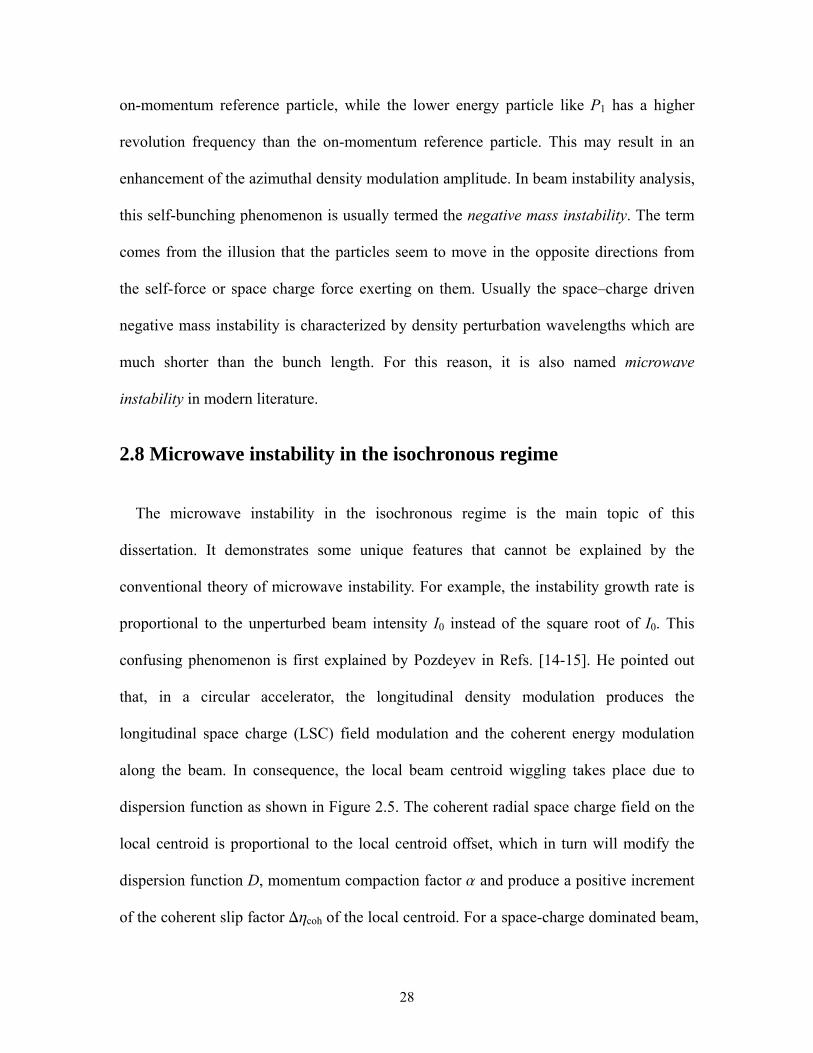
Figure 2.5 Schematic drawing of beam centroid wiggling and the associated coherent space charge fields (The figure is reproduced from Ref. [15])………29
Figure 3.1 A rectangular beam inside a rectangular chamber……………….…………35
Figure 3.2 Comparisons of the on-axis and average LSC impedances between the theoretical calculations and numerical simulations for a beam model of square cross-section inside rectangular chamber with w = 5.7 cm, h =2.4 cm, a = b = 0.5 cm………....................................................................................47
Figure 3.3 Comparisons of the LSC impedances between the square and round models (w=h =rw =3.0 cm, a=b=r0 =0.5 cm)………………………………………..47
Figure 3.4 Simulated LSC impedances of the square and round beam models in a square chamber (w = h =3.0 cm, a = b = r0 = 0.5 cm), respectively……………….48
Figure 3.5 Simulated LSC impedances of a round beam inside square and round chambers (w = h = rw = 3.0 cm, r0 = 0.5 cm), respectively………………...49
xiii
Figure 3.6 LSC impedances of rectangular beam model with different half widths a inside a rectangular chamber (w = 5.7 cm, h = 2.4 cm, a is variable, b = 0.5 cm)………………………………………………………………………….50
Figure 3.7 LSC impedances of a rectangular beam model with different half heights b inside rectangular chamber (w = 5.7 cm, h = 2.4 cm, a = 0.5 cm, b is variable)……………..……………………………………………………...51
Figure 3.8 LSC impedances of square beam model inside rectangular chamber (w = 5.7 cm, h is variable, a = b = 0.5 cm)…………………………..………………51
Figure 3.9 LSC impedances of a square beam model inside a rectangular chamber (w is variable, h = 2.4 cm, a = b = 0.5 cm)…………………………………..…...52
Figure 3.10 A line charge with sinusoidal density modulations between parallel plates…………… ….………………………………………………………57
Figure 3.11 Comparisons of the average LSC impedances of a round SIR beam with beam radius r0=0.5 cm under different boundary conditions and in different
wavelength limits. l is the perturbation wavelength, ,|| is the modulus of LSC impedance. In the legend, ‘Free space’, ‘Round chamber’, and ‘Parallel plates’ are boundary conditions; ‘LW limits’ stands for the long-wavelength limits; ‘(approximation)’ and ‘(simulation)’ stand for the theoretical approximation and simulation (FEM) methods, respectively………………67
Figure 3.12 Comparisons of the average LSC impedances of a round SIR beam with beam radius r0=1.0 cm under different boundary conditions and in different wavelength limits…………………………………………………………...68
Figure 3.13 Comparisons of the average LSC impedances of a round SIR beam with beam radius r0=1.5 cm under different boundary conditions and in different wavelength limits…………..……………………………………………….68
Figure 3.14 Comparisons of the average LSC impedances of a round SIR beam with beam radius r0=2.0 cm under different boundary conditions and in different wavelength limits…..……………………………………………………….69
Figure 3.15 Comparisons of the average LSC impedances of a round SIR beam with beam radius r0=0.5 cm under different boundary conditions and in different wavelength limits. In the legend, ‘Free space’, ‘Round chamber’, and ‘Rect. chamber’ are boundary conditions, where ‘Rect.’ is the abbreviation for ‘Rectangular’; The other symbols and abbreviations are the same as those in Figure 3.11…………………………………………………..……………..72
Figure 3.16 Comparisons of the average LSC impedances of a round SIR beam with beam radius r0=1.0 cm under different boundary conditions and in different wavelength limits…………………………………………………………...72

xiv
Figure 3.17 Comparisons of the average LSC impedances of a round SIR beam with beam radius r0=1.5 cm under different boundary conditions and in different wavelength limits……………...…………..……………………………….73
Figure 3.18 Comparisons of the average LSC impedances of a round SIR beam with beam radius r0 =2.0 cm under different boundary conditions and in different wavelength limits…………………………………………………………..73
Figure 3.19 Comparisons of the average LSC impedances between the round beam and square beam for a parallel plate field model. For a round beam, r0 is the beam radius; for a square beam, r0 is the half length of the side. The square beam model underestimates the LSC impedances………………………………..74
Figure 3.20 Comparisons of the average LSC impedances of a round beam between parallel plates and a round beam inside a round chamber. The round chamber model underestimates the LSC impedances at larger l……………………74
Figure 4.1 Slip factors for I0 = 1.0 mA at s=C0 and s=10C0……………………..……96
Figure 4.2 Slip factors for I0 = 10 mA at s=C0 and s=10C0……………….….………96
Figure 4.3 The E.S.F. at = C0 for a 1.0 mA, 19.9 keV SIR beam. (a) E = 0, and variable emittance. (b) x,0= 50π mm mrad, and variable E……………...98
Figure 4.4 The E.S.F. at = 10C0 for a 1.0 mA, 19.9 keV SIR beam. (a) E=0, and variable emittance. (b) x,0= 50π mm mrad, and variable E……………..98
Figure 4.5 (a) Beam profiles and (b) line density spectrum at turn 0….…………….102
Figure 4.6 (a) Beam profiles and (b) line density spectrum at turn 60………………103
Figure 4.7 (a) Beam profiles and (b) line density spectrum at turn 100……………..103
Figure 4.8 Evolutions of harmonic amplitudes of the normalized line charge densities……………………………………………..……………………..104
Figure 4.9 Curve fitting results for the growth rates of the normalized line charge densities for a single run of CYCO. (a) λ = 0.25 cm; (b) λ = 0.5 cm; (c) λ = 1.0 cm; (d) λ = 2.0 cm; (e) λ = 2.857 cm; (f) λ = 5.0 cm………………...104
Figure 4.10 Comparison of the instability growth rates between theory and simulations for five runs of CYCO……………………………………………………..106
Figure 4.11 Comparisons between the simulated and theoretical normalized instability growth rates for different beam intensities………………………………108
Figure 4.12 Comparisons of microwave instability growth rates between theory and simulations for variable initial emittance………………………………..109
xv
Figure 4.13 Comparisons of microwave instability growth rates between theory and simulations for variable uncorrelated RMS energy spread……………...110
Figure 5.1 Schematic of a basic parallel-plate RFA. (b) Ideal I-V characteristic curve with V2=V0 for monoenergetic particles (c) Usual I-V characteristic cutoff curve. The slope between V =V0-DV and V=V0 is due to the trajectory effect. The effect of secondary electron emission is shown in the dotted curve. (Note: the figure is reproduced from Ref. [48])… ………………………..……115
Figure 5.2 Comparison of the measured energy spectra for electron beamlet with two different currents inside the analyzer. Curve I is for the current of 0.2 mA, the RMS energy spread is 2.2 eV; Curve II is for the current of 2.6 mA, the RMS energy spread is 3.2 eV. (Note: the figure is cited from Ref. [50])……....118
Figure 5.3 A Schematic of the Measurement Box.‘Phos. Screen’, ‘E. A’ and ‘Med. Plane’ stand for the ‘Phosphor Screen’, ‘Energy Analyzer’ and ‘Median Plane’, respectively…………………………………………………………….. .119
Figure 5.4 A schematic of the SIR energy analyzer with a horizontally (radially) expanded beam. The beam (green oval) is moving towards the analyzer (into the paper). The analyzer can scan back and forth along the ring radius. The thin yellow rectangle in the middle of the analyzer depicts a sampled beam slice or beamlet……………………………………………………..……120
Figure 5.5 Schematic of the 2nd generation UMER energy analyzer. (a) Field model and simulated trajectories (left). (b) Mechanical structure (right). (Note: the figure is cited from Ref. [51])……………………………………………..121
Figure 5.6 Schematic of the 3rd generation UMER energy analyzer. (a) Field model and simulated trajectories (left). (b) Electronic circuit (right). (Note: the figure is cited from Ref. [52])………………………………………………………121
Figure 5.7 The movable small mesh model (left) and simulated particle trajectories (right).……………………………………………………………………126
Figure 5.8 Two schematics of the SIR energy analyzer and particle trajectories simulated by SIMIOM, where the beam energy is 20.01 keV, the voltages of the regarding mesh and suppressor are Vretarding=20 kV and Vsuppressor=-300V, respectively………………………………………………………………127
Figure 5.9 Performance of the SIR analyzer simulated by SIMION 8.0 for a fixed retarding potential Vretarding =20 kV and variable source voltage Vsource……………………………………………………………………..128
Figure 5.10 The photos of the SIR energy analyzer………………...………………….129
Figure 5.11 Schematic of the ARTEMIS-B Ion Source beam line. The performance test of the SIR analyzer was carried out in the diagnostic chamber indicated by the
xvi
red arrow……….………………………………………………………..130
Figure 5.12 Performance of the SIR energy analyzer tested at ARTEMIS-B ECR ion source……………..…………………………………………………….....131
Figure 5.13 Performance of the SIR energy analyzer tested at SIR by DC beam……...131
Figure 6.1 Schematic of the energy spread measurement system…………..……...…134
Figure 6.2 Energy analyzer assembly including the supporting rod, flange, and motor drive (left) and motor controller (right)………..………………………..135
Figure 6.3 Energy analyzer assembly in the SIR (left) and a side view with the Extraction Box (right)……………………………………………………..135
Figure 6.4 Preamplifier (TENNELEC TC-171) (left) and Amplifier (TENNELEC TC-241S) (right)………………….……………………………………. ...135
Figure 6.5 High voltage power supply (BERTAN 225) for the retarding grid (left) and oscilloscope (LeCroy LC684DXL) (right)……………..…………………136
Figure 6.6 A sample of the energy spread analysis at turn 10. The upper graph shows the comparison between the original and reconstructed S-V curves. The lower graph displays the fitted Gaussian distribution of beam energy. The mean kinetic energy, RMS and FWHM energy spreads are 10118.7 eV, 44.75 eV and 105.2 eV, respectively…………………………………………………138
Figure 6.7 Evolutions of the radial beam density………………………..………….140
Figure 6.8 Simulated top views and slice RMS energy spread at (a) turn 4 (b) turn 30………………………………………………..........................................141
Figure 6.9 Simulated slice RMS energy spread at turns 0-8……………….…..……141
Figure 6.10 Comparisons of slice RMS energy spread between simulations and experiments ……………………………………………………………….142
Figure 6.11 Sketch of clusters and energy analyzer…….……………………………143
Figure 6.12 Corotation of two macroparticles with Q=8ä10-14 Coulomb, E0 = 10.3 keV, and d0=1.5 cm………………………..…………………………..146
Figure 6.13 Simulated distance between the two particles (left) and their corotation angle with respect to the +z-coordinate (right) in the first corotation period. The simulated corotation frequency wsim can be fitted from the angle-turn number curve. The theoretical corotation frequency wthr predicted by Eq. (6.10) is also plotted for comparison………………………………………………148
Figure 6.14 Simulated corotation frequencies of two macroparticles with different initial

xvii
distance d0…………………………………………………………………148
Figure 6.15 Corotation of two short bunches with tb=10 ns, I0=8.0 uA, Q=8ä10-14 Coulomb, d0=1.5 cm, and E0 = 10.3 keV………………………………...149
Figure 6.16 Simulated distance between the centroids of two short bunches (left) and their angle with respect to the z-coordinate (right) in the first 1/4 corotation period. The simulated corotation frequency wsim and the theoretical value wthr predicted by Eq. (6.10) are also provided in the right graph………………150
Figure 6.17 Initial distribution of 2D bunch pair with tb=10 ns, I0=8.0 uA, Q=8ä10-14 Coulomb, E0=10.3 keV and d0=1.5 cm. The upper graph shows the top view of the beam profile in z-x plane; the lower graph shows the side view of the beam in z-y plane.………………………………………………………….151
Figure 6.18 Beam profiles of 2D bunch pair in the center of mass frame at turn 2……151
Figure 6.19 Beam profiles of 2D bunch pair in the center of mass frame at turn 5……152
Figure 6.20 Beam profiles of 2D bunch pair in the center of mass frame at turn 12…...152
Figure 6.21 Beam profiles of 2D bunch pair in the center of mass frame at turn 20…..153
Figure 6.22 Beam profiles of the 2D bunch pair in the center of mass frame at turn 30. …………………………………………………………………............153
Figure A.1 Schematic of a half cell of an N-fold symmetric isochronous ring. The ring center is located at point O. r0 and r1 are the bending radii of the on-momentum and off-momentum particles with their centers of gyration located at points A and B, respectively. The solid line passing points P and U depicts the titled pole face of the magnet. l and l1 are the half drift lengths traveled by the on-momentum and off-momentum particles, respectively..164
Figure A.2 Schematic of the SIR lattice……………………………………………….167
Figure A.3 Schematic of the optics functions v.s distance S of a single period of the SIR lattice calculated using transfer matrices…………………………………170
1
Chapter 1
INTRODUCTION
Isochronous cyclotron is an important family member of modern particle accelerators,
with a relatively compact structure and ability of being operated in continuous wave (CW)
mode. Using a fixed accelerating frequency, it can accelerate the high intensity hadron
beams to medium energy efficiently, typically ranging from several tens of MeV to
several hundred MeV. Now isochronous cyclotrons are widely used in various fields and
applications, such as research in nuclear physics, medical imaging, radiation therapy and
industry, etc.
Since the 1980’s, the successful operation of the high power Ring Cyclotron (capable
of producing a proton beam of 2.4 mA, 590 MeV with a power of 1.4 MW) at Paul
Sherrer Institute (PSI) in Switzerland has greatly inspired the cyclotron community.
Consequently, the possibility of design and operation of more powerful cyclotrons
(typically, 1 GeV, 10 mA, 10 MW) have been discussed extensively and proposed in
some new applications, such as accelerator driven subcritical reactors (ADSR),
transmutation of nuclear waste and energy production, neutrino Physics [1-5], etc. M.
Seidel provided an excellent review on cyclotrons for high intensity beams [6], their
working principles, limitations in the design and operation were briefly introduced. This
dissertation mainly discusses the microwave instability of low energy, high intensity
beams in isochronous regime induced by space charge effects which is a key issue for the
performance of high power cyclotrons.
2
1.1 Brief introduction to cyclotrons
The first classical cyclotron was proposed and designed by E. O. Lawrence in the early
1930s, in which charged particles move in a vertically uniform magnetic field with a
constant revolution frequency (cyclotron frequency). An electric field with fixed radio
frequency (RF), which is equal to the cyclotron frequency between two D-shaped
electrodes (the Dees), is utilized to accelerate the particles multiple times resonantly to
high energy. In order to overcome the energy limits posed by the phase slippage due to
relativistic effects and vertical focusing, in 1938, L. H. Thomas proposed the concept of
radial sector focusing isochronous cyclotron of which the radially increasing magnetic
fields provide isochronism, and the azimuthally varying magnetic fields (AVF) provide
vertical focusing (Thomas focusing). In addition, many modern isochronous cyclotrons
adopt spiral-shaped sectors which may enhance the vertical focusing further. The
accelerated beam can be extracted by some popular methods, such as resonance
extraction, stripping extraction for H- ions, etc.
1.2 Space charge effects in isochronous cyclotrons
When the beam intensity increases in isochronous cyclotrons, the collective effects of
the repulsive Coulomb force among the charged particles, which are usually termed space
charge effects, become vital factors for the highest intensity attainable in the machine.
Refs. [6-7] provide enlightening reviews and discussions regarding the space charge
effects in isochronous accelerators.
The space charge effects can be classified into two major categories: incoherent
transverse effects and coherent radial-longitudinal ones.
3
1.2.1 The incoherent transverse space charge field
The incoherent transverse space charge field can decrease the vertical focusing
resulting in negative incoherent tune shifts which are proportional to the beam current
and 1/23 [8], where and are the relativistic speed and energy factors, respectively.
Usually, in the central region of isochronous cyclotrons, the vertical focusing force
provided by the azimuthally varying magnetic fields (Thomas force) is weaker, thus a
beam of high intensity and low energy may have a large tune shift and vertical beam size.
The vertical chamber size sets the upper limits for the beam intensity. Higher injection
energy is preferred to mitigate the incoherent transverse space charge effects.
1.2.2 The coherent radial-longitudinal space charge field
Different from the incoherent transverse space charge effects which are common for all
types of accelerators, the coherent radial-longitudinal space charge effects in isochronous
cyclotrons demonstrate some characteristics that are unique in isochronous regime. The
longitudinal space charge (LSC) fields within a bunch of finite length may induce energy
spread among the charged particles. In isochronous regime, since the longitudinal motion
is frozen, particles with higher (or lower) energy must have longer (or shorter) path
lengths and larger (or smaller) gyroradii to maintain a constant revolution frequency. This
may result in the vortex motion and an S-shaped beam, the narrowed turn separation
makes clean extraction difficult. For higher power cyclotrons, considerable number of
particles hitting the extraction deflectors may cause serious beam loss, overheating and
activation of extraction device. The required low extraction loss rate is the limiting factor
for the attainable beam intensity in high power isochronous cyclotrons.
4
More comprehensive knowledge and deeper understanding of space charge effects are
crucial for the successful design and operation of high power isochronous cyclotrons. In
the past decades, additional extensive studies on this topic have been done through
numerical simulations, experiments and analytical models.
1.2.3 Vortex motion
Gordon is the first researcher who explained that the vortex motion in isochronous
cyclotrons originates from the space charge force [9], which is equal to half of the
Coriolis force seen by a particle in a reference frame rotating with constant angular
frequency c
in the isochronous magnetic field
,scc Eqvm
(1.1)
where m and q are the mass and charge of the particle, respectively, v
is the speed of
particle in the rotating frame, and scE
is the space charge field, c
is the cyclotron
frequency vector
.m
Bqc
(1.2)
Another half of the Coriolis force in the rotating frame cancels the centrifugal force and
Lorentz force on the particle. Cerfon [10] interpreted the vortex motion in isochronous
regime as nonlinear convection of beam density in the × velocity field
.2B
BEv sc
(1.3)
Since the cyclotron frequency vector c
is proportional to the isochronous magnetic
field vector as shown in Eq. (1.2), in fact, the two different interpretations of vortex
5
motion described in Eqs. (1.1) and (1.3) are equivalent to each other essentially. It can be
verified easily by plugging Eqs. (1.2) and (1.3) into Eq. (1.1).
1.2.4 Space charge effects and stability of short circular bunch
By using a closed set of differential equations for the second-order moments of the
phase space distribution functions, taking into account the space charge effects,
neglecting the force from the image charges and neighboring turns, Kleeven [11] proved
that a single free bunch with a circular horizontal cross-section is stationary in a AVF
isochronous cyclotron; for a beam with non-circular horizontal initial cross-section, it
will not be stable until it evolves to a circular one. This property has been verified and
utilized in the successful operation of PSI Injector II, where a buncher is used to produce
small round bunches with energy of 870 keV before they are injected into and accelerated
in the Injector II. Because the shape of short bunches can barely change during
acceleration, a large enough turn separation can be achieved at extraction energy of 72
MeV with high extraction rate (~99.98%). Cerfon [10] also verified and explained this
phenomenon by both theory and simulations as discussed in Sect. 1.2.3.
1.2.5 Space charge effects of long coasting bunch
The simulation and experimental work done by Pozdeyev and Rodriguez [12-15]
showed that, when a high intensity long bunch with initially uniform longitudinal charge
distribution is injected into the Small Isochronous Ring, it may break up into some small
clusters longitudinally after only several turns of coasting. Later those small clusters
coalesce by consecutive binary cluster merging process. The fast clustering process

6
observed in simulations and experiments is just the microwave instability of a
space-charge dominated beam.
1.2.6 Space charge effects between neighboring turns
For high intensity cyclotrons, the turn separation decreases at high energy.
Consequently, the space charge effects contributed from the radially neighboring turns
must be considered in the beam dynamics.
Using a 3D parallel Particle-In-Cell (PIC) simulation code OPAL-CYCL, a flavor of
the Object Oriented Parallel Accelerator Library (OPAL) framework developed by
Adelmann of PSI [17], the space charge effects between neighboring turns in the PSI 590
MeV Ring Cyclotron were simulated by Yang adopting a self-consistent algorithm [18].
The simulation results show that there is a considerable difference between single-bunch
and multi-bunch dynamics. The space charge forces contributing from the radially
neighboring turns may ‘squeeze’ the radial beam size to some extents and play a positive
role in maintaining turn separation and reducing the energy spread.
From the above information, we can see it is challenging to design and operate a high
intensity cyclotron keeping a low level of beam loss and activation. The effects of an
incoherent transverse space charge field, a coherent radial-longitudinal space charge field
and neighboring turns are crucial factors thus must be taken into account. This requires a
better understanding and manipulation of the space charge effects in isochronous regime.
1.3 CYCO and Small Isochronous Ring
Usually it is difficult to study analytically the beam dynamics with space charge in
7
isochronous ring due to complex boundary conditions of the accelerator, nonlinear effects
resulting from beam shape and distributions. Thus, the numerical method using
simulation codes and experimental method utilizing a real isochronous accelerator are
heavily relied upon in the research.
Since the beam dynamics of the existing simulation codes were then simplified in the
treatment of space charge effects, Pozdeyev developed a novel 3D Particle-In-Cell
simulation code named CYCO to study the beam dynamics with space charge in
isochronous regime [12]. In the simulation, at first, an initial distribution of a number of
macroparticles (typically 3 ä 105) representing the real long ion bunch (typically 40 cm
long) needs to be created either by the code with a default distribution or by users’
self-definition. Using the classical 4th order Runge-Kutta method, the code can
numerically solve the complete and self-consistent system of six equations of motion of
the charged macroparticles in a realistic 3D field map including the space charge fields.
Because of the large aspect ratio between the vacuum chamber width and height of the
storage ring, the code only includes the image charge effects in the vertical direction. The
rectangular vacuum chamber is simplified as a pair of infinitely large, ideally conducting
plates parallel to the median ring plane. The beam profiles can be output turn by turn for
post-processing and analysis.
In order to validate the simulation code CYCO and study the space charge effects in
the isochronous regime, a low energy, low beam intensity Small Isochronous Ring (SIR)
was constructed during 2001-2004 at the National Superconducting Cyclotron Laboratory
(NSCL) at Michigan State University (MSU). In addition, two graduate students
Pozdeyev and Rodriguez conducted a thesis project and the SIR has been in operation
until
energ
comp
scale
loose
availa
study
Th
sourc
are li
2010 [12-1
gy, low inten
pact accelera
, high power
e requiremen
ability and f
y the space c
he Small Iso
ce, an injecti
sted in Table
Figure 1
3]. Accordin
nsity H2+ be
ator ring can
r isochronou
nts of time
flexibility in
harge effects
chronous Ri
ion line, and
e 1.1.
1.1: A photo
ng to the sc
eam in SIR
n be used to
us cyclotrons
e resolution
n the operati
s in the isoch
ing consists
d a storage r
graph of the
8
caling laws,
covers a la
o simulate t
s such as the
and beam
ion, the SIR
hronous regi
of three ma
ring as show
SIR with so
the space c
arge region
the space ch
e PSI Injecto
m power for
R is an ideal
ime.
ain parts: a m
wn in Figure
ome key elem
charge regim
in beam dy
harge effects
or II cyclotro
r diagnostic
l experimen
multi-cusp H
1.1. Its mai
ments indica
me of the low
ynamics. Th
s of the larg
on. Due to th
c tools, goo
ntal facility t
Hydrogen io
in parameter
ated.
w
is
ge
he
od
to
on
rs
9
Table 1.1: Main parameters of SIR
Ring circumference 6.58 m Particle species H+, H2
+, H3+, mainly use H2
+ Kinetic energy 0 -30 keV Peak current 0-40 mA for H2
+ RMS emittance Typically 2-3 mm mrad
Ring lattice Four 90-degree dipole magnets Bending radius 0.45 m
Dipole pole face angle 26o Mag. field strength 800 Gauss
Bare horizontal tune nx 1.14 Bare vertical tune ny 1.11
Bare slip factor 0 ~2.0 ä 10-4 Beam life time ~200 turns
The ion source produces three species of Hydrogen ions: H+, H2+, and H3
+. An
analyzing dipole magnet under the ion source is used as a magnetic mass separator to
select the H2+ ions which are usually used in the experiments. The H2
+ ion beam with
proper Courant-Snyder parameters and desired bunch length can be produced by an
electrostatic quadrupole triplet and chopper in the injection line. The storage ring has a
circumference of 6.58 meter. It mainly consists of four identical flat-field 90o bending
magnets with edge focusing. The pole faces of each magnet are rotated by 26o in order to
provide both the vertical focusing and isochronism at the same time. After being injected
to the storage ring by two fast-pulsed electrostatic inflectors (Inflector 1 and Inflector 2 in
Figure 1.1), the bunch may coast in the ring up to 200 turns. There is a Measurement Box
located in the drift line between the 2nd and 3rd bending magnets in the ring. A pair of
fast-pulsed electrostatic deflector in the Measurement Box can kick the beam either up to
a phosphor screen above the median ring plane, or down to the fast Faraday cup (FFC)
below the median ring plane. The phosphor screen and fast Faraday cup are used to
monitor the transverse and longitudinal beam profiles, respectively. We can also perform
10
energy spread measurements if the fast Faraday cup assembly is replaced by an energy
analyzer assembly.
A double-slit emittance measurement assembly is located in the Emittance Box of the
injection line. It is used to measure the RMS emittance in horizontal and vertical phase
space. An Einzel Lenz right under the ion source can focus the divergent beam. Together
with the electrostatic quadrupole triplet in the injection line, users can obtain the proper
Courant-Snyder parameters. A shielded Faraday cup at the end of the injection line is
used to measure the beam current when the Inflector 1 is turned off. Two pairs of
horizontal and vertical scanning wires are installed in the storage ring to monitor the
transverse beam profiles. In order to adjust the betatron tunes and isochronism, four
electrostatic quadrupoles and four gradient correctors are installed in the ring between the
bending magnets and situated in the dipole magnets, respectively.
1.4 Summaries of previous studies of beam instability in SIR
It was observed both in simulations by CYCO and experiments at SIR, a coasting long
bunch with uniform longitudinal charge density may develop a fast growth of density
modulation. The whole bunch breaks up into many small clusters in the longitudinal
direction quickly. Furthermore, the neighboring small clusters may merge together to
form bigger ones by a consecutive binary merging process. Figure 1.2 shows the
measured temporal evolutions of the longitudinal bunch profiles of a coasting beam with
the beam energy of 20.9 MeV and the peak current of 9.3 A [15]. Figure 1.3 shows the
simulation results of the beam dynamics in SIR for three different peak intensities: 5 A,
10 A, and 20 A [13].
Figurinjectturn 2
Figurdensi
re 1.2: Longtion (turn 0)20 are shifte
re 1.3: Simuities: 5 A, 1
gitudinal bu), at turn 10d vertically
ulation resu10 A, and 2
unch profiles0 and turn 2by 0.3 and 0
lts of the b20 A [13].
11
s measured 0. The curre
0.6, respectiv
beam dynam
by the fastent profiles vely [15].
mics in SIR
t Faraday cumeasured a
for three d
up right afteat turn 10 an
different pea
er nd
ak

12
In order to study the dependence of beam instability on various initial beam parameters,
Rodriguez carried out extensive simulations and experimental studies [13]. He studied the
temporal evolutions of the number of clusters by means of the cluster-counting technique.
The simulation and experimental results agreed to each other quite well. Finally, several
scaling laws of instability growth rates with respect to the various beam parameters (e.g.,
the beam current, energy, emittance and bunch length) were set up empirically. It was
found that the instability growth rates are proportional to the beam current instead of the
square root of beam current. This property contradicts the prediction by the conventional
theory of microwave instability. Rodriguez also counted the decreasing number of
clusters and fit it to an empirical exponential function of turns.
Pozdeyev explained [14-15] that the centroid wiggling of a long bunch in isochronous
ring plays an important role in the microwave instability. It may produce coherent radial
space charge fields, modify the dispersion function and coherent slip factor, raise the
working point above transition and enhance the negative mass instability. Plugging the
modified coherent slip factor into the conventional 1D formula for microwave instability
growth rates, Pozdeyev derived an instability formula which can predict the linear
dependence of instability growth rates on beam current. While this model overestimates
the growth rate of short-wavelength perturbations. Later, Bi [16] proposed another model
consisting of a round perturbed beam inside a round chamber. This model takes into
account the effect of centroid offsets on transition gamma. Bi derived a 1D dispersion
relation that can predict the fastest-growing mode and explain the various scaling laws.
But this model is not consistent with the scaling laws on beam current, since the DC
current component is neglected in calculating the coherent radial space charge field.

13
1.5 Major research results and conclusions in this dissertation
In spite of the pioneering work done by Pozdeyev, Rodriguez and Bi [12-16], some
central questions still remain in regard to the more accurate, comprehensive and deeper
understanding of the microwave instability in isochronous regime. For example,
(a) None of Pozdeyev [14-15] and Bi’s theoretical models [16] utilized the longitudinal
space charge (LSC) field and impedance models that exactly match the geometries of the
real beam-chamber system and can work at any perturbation wavelengths. The validity of
their LSC field and impedance models needs to be verified. It is highly desirable for the
beam physicists to obtain the analytical LSC impedances for a round beam with
sinusoidal density modulations inside a rectangular chamber, or between parallel plates
(e.g., in CYCO). Moreover, the derived LSC impedances should be accurate enough at
any perturbation wavelengths.
(b) Is the 1D growth rate formula or dispersion relation adopted by Pozdeyev [14-15]
and Bi [16] accurate enough to predict the instability growth rates at any wavelengths?
How do the energy spread and emittance neglected in their models affect the instability
growth rates? How to introduce the well-known Landau damping effects in the
isochronous regime?
(c) How does the energy spread of clusters evolve? What is the asymptotic behavior of
the energy spread and why? How and why the cluster pair merge?
This dissertation primarily discusses and answers the above questions. To predict the
microwave instability growth rates more accurately, this dissertation
(1) derives the analytical LSC impedances of a rectangular and round beam inside a
rectangular chamber and between parallel plates;
14
(2) derives a 2D dispersion relation incorporating the Landau damping effects
contributed from finite energy spread and emittance. It can explain the suppression of
microwave instability growth rates at short perturbation wavelengths and predict the
fastest-growing wavelength;
(3) studies the evolution of energy spread of SIR bunch by both simulation and
experimental methods. We have designed a compact rectangular electrostatic retarding
field analyzer [19] with a large entrance slit. The simulation and experimental studies of
energy spread evolution of a long coasting bunch show that the slice RMS energy spread
of clusters changes slowly at large turn numbers. This may result from nonlinear
advection of the beam in the × velocity field [10].
1.6 Brief introduction to contents of the following chapters
Chapter 2 gives a brief introduction to some most important concepts and dynamics
regarding the isochronous ring, including the momentum compaction factor, dispersion
function, slip factor, beam optics of SIR lattice (hard-edge model), microwave instability,
Landau damping, etc.
Chapter 3 derives the analytical LSC fields and impedances of (a) a rectangular beam
and (b) a round beam with planar and rectangular boundary conditions, respectively. The
derived LSC impedances match well with the numerical simulations. We study the effects
of the cross-sectional geometries of both the beam and chambers on the LSC impedances.
Chapter 4 discusses the Landau damping effects of a coasting long bunch in the SIR.
The limits of the conventional 1D formalisms used in the existing models are pointed out;
a modified 2D dispersion relation suitable for the beam dynamics in the isochronous
15
regime is derived, by which the Landau damping effects are studied. It can explain the
suppression of instability growth and predict the fastest-growing wavelength.
Chapter 5 introduces the working principles, simulation design, and mechanical
structure of a rectangular retarding field energy analyzer with large entrance slit. The
dissertation provides the tested performance and sensitivity of the analyzer.
Chapter 6 is devoted to studying the nonlinear beam dynamics of the microwave
instability, including (a) energy spread measurements and simulations. First, this chapter
gives a brief introduction to the measurement system, and then the measurement and data
analysis methods. The simulation and experimental results are compared with each other;
their physical meaning is interpreted by simple analysis. (b) verification of Cerfon’s
theory [10] on the vortex motion in × field by two-macroparticle model and
two-bunch model.
Chapter 7 summarizes the main research results addressed in this dissertation and
points out some possible research directions in the future.
For
chapt
essen
2.1 T
In t
for th
accel
Figurradialrefere
The
wher
refere
BAS
r the conven
ters, this ch
ntial in under
The accel
this disserta
he SIR. Fig
erator mode
re 2.1: A siml, vertical anence particle
e SIR is assu
e R is the av
ence particle
SIC CON
nience of fu
hapter briefly
rstanding the
lerator m
ation, the sam
gure 2.1 sho
el.
mplified accnd longitudi
e O. (Note: th
umed to be a
verage ring r
e O within th
Ch
NCEPTS
urther discus
y summariz
e unique bea
odel for t
me accelerat
ows the sch
celerator moinal coordinhe figure is r
an ideal circu
radius. A bea
he bunch cir
16
hapter 2
AND BE
ssions on mi
zes some ba
am dynamics
the SIR
tor model as
hematic view
del for the Snates of the reproduced f
ular storage
am is coastin
culates along
EAM DY
icrowave ins
asic but imp
s in the isoch
s the one use
w of the co
SIR, in whiccharged par
from Ref. [2
ring with a c
ng in the rin
g the design
YNAMIC
stability in t
portant conc
hronous regi
ed in Ref. [2
oordinate sy
ch x, y, andrticle with r
20]).
circumferen
ng. Assume a
n orbit turn a
CS
the followin
cepts that ar
ime.
20] is adopte
ystem for th
d z denote threspect to th
ce of C0=2p
a hypothetica
after turn wit
ng
re
ed
he
he he
pR,
al
th

17
the exact design energy 2
2cmE
H , where g is the relativistic energy factor of the
on-momentum particle, 2H
m is the rest mass of the Hydrogen molecular ion 2H , c is the
speed of light. The reference particle has a velocity of v=bc, where b is the relativistic
speed factor. The distance traveled by the reference particle with respect to a fixed point
of the storage ring is s=vt=bct. For an arbitrary particle in the bunch, x, y, and z denote its
radial, vertical and longitudinal coordinates with respect to the reference particle O,
respectively. Then the motion of an arbitrary particle can be described by a
six-component vector (x, x£, y, y£, z, d) in phase space, where x£=dx/ds, and y£=dy/ds are
the radial and vertical velocity slopes relative to the ideal orbit, d=Dp/p is the fractional
momentum deviation. For a coasting SIR beam, we can choose a hypothetical
on-momentum particle at the bunch center as the reference particle. For those
off-momentum particles in a circular accelerator, there are three important parameters
describing their motions: momentum compaction factor a, dispersion function D(s) and
phase slip factor h.
2.2 Momentum compaction factor
In a circular accelerator, the particles of different energy circulate around different
closed orbits resulting in different path length C and different equilibrium radius. In beam
dynamics, the ratio between the fractional path length deviation DC/C0 (or fractional
equilibrium radius deviation DR/R) and the fractional momentum deviation d=Dp/p is
customarily defined as the momentum compaction factor:
./
/
/
/ 0
pp
RR
pp
CC
(2.1)
18
It is a measure for the change in equilibrium radius due to the change in momentum.
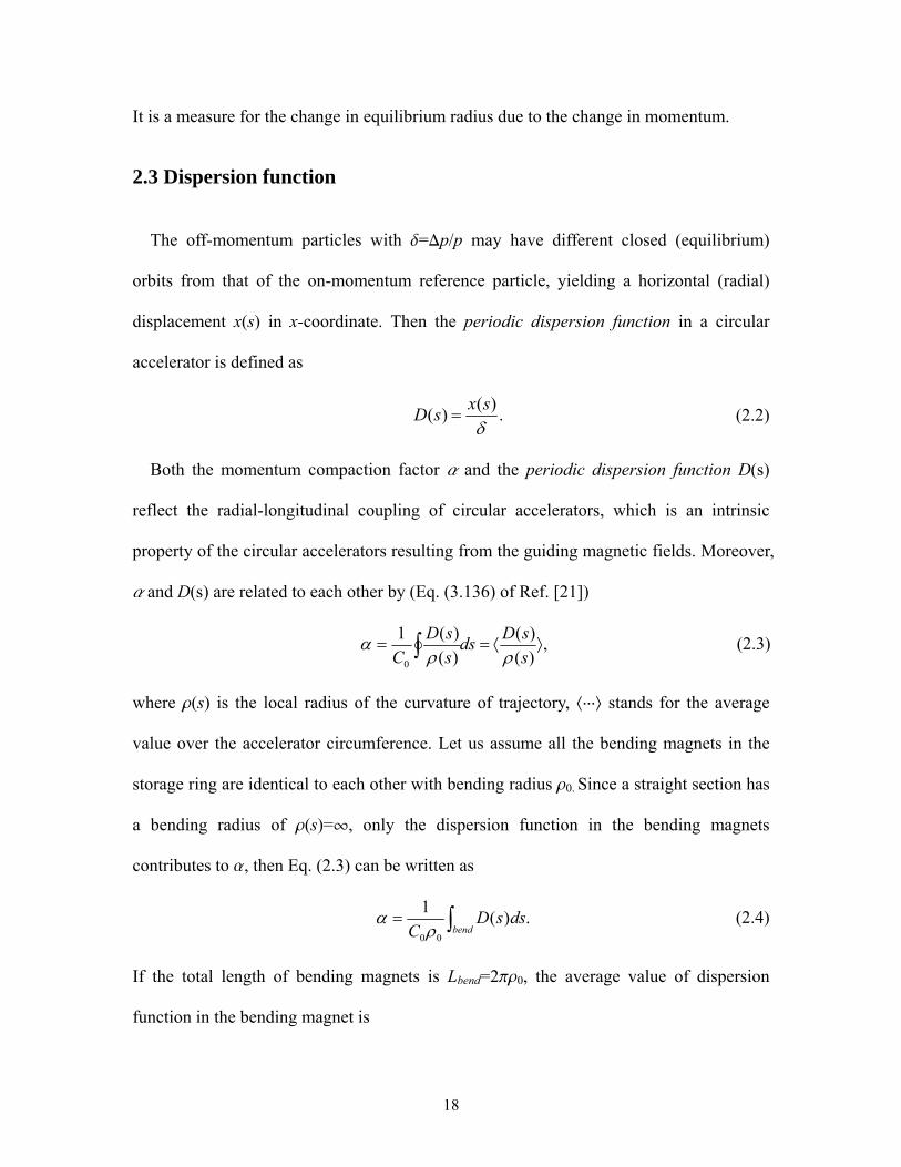
2.3 Dispersion function
The off-momentum particles with d=Dp/p may have different closed (equilibrium)
orbits from that of the on-momentum reference particle, yielding a horizontal (radial)
displacement x(s) in x-coordinate. Then the periodic dispersion function in a circular
accelerator is defined as
.)(
)(sx
sD (2.2)
Both the momentum compaction factor a and the periodic dispersion function D(s)
reflect the radial-longitudinal coupling of circular accelerators, which is an intrinsic
property of the circular accelerators resulting from the guiding magnetic fields. Moreover,
a and D(s) are related to each other by (Eq. (3.136) of Ref. [21])
,)(
)(
)(
)(1
0
s
sDds
s
sD
C (2.3)
where r(s) is the local radius of the curvature of trajectory, ‚ÿÿÿÚ stands for the average
value over the accelerator circumference. Let us assume all the bending magnets in the
storage ring are identical to each other with bending radius r0. Since a straight section has
a bending radius of r(s)=¶, only the dispersion function in the bending magnets
contributes to a, then Eq. (2.3) can be written as
.)(1
00
benddssD
C (2.4)
If the total length of bending magnets is Lbend=2pr0, the average value of dispersion
function in the bending magnet is

19
.)(2
1)(
0
bendbend dssDsD
(2.5)
Then Eq. (2.4) reduces to
.)()(2
00
0
R
sD
C
sD bendbend
(2.6)
where R=C0/2p is the average ring radius.
2.4 Transition gamma
The transition gamma gt in circular accelerators is defined as
./
/2
RR
ppt
(2.7)
It is easy to learn from Eq. (2.1) and Eq. (2.7) that
.1
2t
(2.8)
The total energy of a particle with transition gamma is just the transition energy which is
equal to .2mcE tt
2.5 Slip factor
The revolution period of a particle is cRT /2 , the fractional deviations of the
relativistic speed and momentum are related by 2// , then with Eq. (2.7),
,)11
(- 2200
tR
R
T
T (2.9)
where T0 and w0 are the revolution period and angular revolution frequency of the
on-momentum reference particles, respectively, h is the phase slip factor defined as
20
.1
-11
222
t
(2.10)
For the SIR, the bare slip factor without the space charge effect is h0º2ä10-4
.
The revolution time and frequency of an off-momentum particle is determined by its
changes in both velocity and path length. A particle with higher energy (d>0) has a faster
velocity and travels along a longer path length compared with the on-momentum
reference particle (d=0). For the case of g<gt, below the transition, h<0, the faster speed
of the higher energy particle (d>0) may compensate for the longer path, this will result in
a shorter revolution period (DT<0 in Eq. (2.9)) or higher revolution frequency (Dw>0 in
Eq. (2.9)) compared with the on-momentum reference particle. While for the case of g>gt,
above the transition, h>0, the increase of path length of the higher energy particle (d>0)
may dominate over the increase of velocity. This will result in a longer revolution period
(DT>0 in Eq. (2.9)) or lower revolution frequency (Dw<0 in Eq. (2.9)) compared with the
on-momentum reference particle.
At transition, g=gt, h=0, the revolution period (or frequency) of the particle is
independent of its energy (or momentum). For a coasting bunch, if the space charge
effects among the particles are excluded, all the particles with different energy will
circulate along the accelerator rigidly with the same period (or frequency). This is the
isochronous regime, in which the Small Isochronous Ring (SIR) is designed to be
operated. Unfortunately, this is a regime which is most vulnerable to the perturbations
and prone to beam instability for a space-charge dominated beam.
2.6 Beam optics for hard-edge model of SIR
Figure 2.2 depicts the layout of the SIR lattice. In consists of four 90-degree bending

magn
bendi
Tab
the te
Fig
s of a
nets (B1-B4)
ing magnet i
Number of
Bending
Drift l
ble 2.1 lists
erm ‘hard–ed
gure 2.3 sho
a single perio
) connected b
is rotated by
Fig
Table 2.
f magnets N
g radius r0
length L
the main par
dge’ means a
ows the simu
od of the ring
by four strai
y an angle j f
gure 2.2: Lay
1: Paramete
N 4
0.45 m
0.79714 m
rameters of t
all the fringe
ulated optica
g calculated
21
ight drift sec
for isochron
yout of the S
rs of SIR (ha
Rotation
Hor
m V
the hard-edg
e magnetic fi
al functions
by code DIM
ctions (S1-S
nism and vert
SIR lattice.
ard-edge mo
n angle of po
rizontal tune
Vertical tune
ge model of
ields are neg
( ), (MAD.
S4). The pole
tical focusin
odel)
ole face j 2
e nx
ny
the SIR latti
glected.
), and Dx(s
e face of eac
ng.
25.159o
1.14
1.17
ice [12]. Her
s) v.s distanc
ch
re
ce

Figurrectan‘BET( )repro
Th
in a
(close
perfo
fracti
by th
ring,
wher
veloc
off-m
re 2.3: The ngle schema
TY’, and ‘D) , and horioduced from
he design of
bunch with
ed) orbits w
orm betatron
ional momen
he red dashed
the followin
e L, P are t
city v, resp
momentum p
optical funcatically showX’ stand forizontal dispRef. [12]).
SIR by the h
h different e
with the sam
n oscillations
ntum deviati
d line in Fig
ng equality s
the straight
pectively. L
article. Eq. (
ctions v.s disws one of tr the horizo
persion func
hard-edge m
energy devia
me nominal
s. Let us as
ion d=Dp/p>
gure 2.2. In o
hould hold
v
PL
and curved
L1, P1 and
(2.11) dictate
22
stance of a the dipole montal beta fuction Dx(s),
model is base
ations travel
l revolution
ssume a non
>0 travels al
order to obta
1
11
v
PLP
path length
v1 are the
es the rotatio
single periomagnets. Thunction (
respectively
ed on the ass
l along thei
n period T0.
n-relativistic
long its equi
ain isochron
h of the on-
e correspon
on angle of p
od of the rinhe legend ite), vertical y. (Note: T
sumption: al
ir individua
These part
c particle wi
ilibrium orb
nism, in one
-momentum
nding quant
pole face [12
ng. The blacems ‘BETXbeta functio
The figure
l the particle
al equilibrium
ticles do no
ith a positiv
bit as indicte
period of th
(2.11
particle wit
tities of th
2]
ck X’, on is
es
m
ot
ve
ed
he
1)
th
he

23
.
)4
tan(
2/2/
)tan(
0
LL
(2.12)
By smooth approximation, the design orbit of SIR lattice can be treated as an ideal
circle with average radius R as indicated by the blue dashed circle in Figure 2.2.
Neglecting the vertical motion, the Hamiltonian of a single particle coasting in SIR
without space charge field and applied electric field is
,222 2
222
R
xxkxH x (2.13)
where kx is the radial (horizontal) focusing strength. According to the Hamiltonian
mechanics,
,x
H
ds
dx
,
x
H
ds
xd
,
H
ds
dz ,
z
H
ds
d
(2.14)
the equations of motion of a single particle are
Radial (horizontal): ,xds
dx ,'
Rxk
ds
dxx
(2.15)
Longitudinal: ,2
R
x
ds
dz .0
ds
d (2.16)
The two radial equations of motion in Eq. (2.15) can also be combined as
.2
2
Rxk
ds
xdx
(2.17)
Using smooth approximation,2
2
Rk x
x
, where nx is the radial (horizontal) betatron tune,
Eq. (2.17) can be rewritten as
.2
2
2
2
Rx
Rds
xd x (2.18)

24
Its general solution is
,)sin()cos()(2
x
xx Rs
RBs
R
vAsx (2.19)
),cos()sin(-)( sRR
BsR
v
RAsx xxxx
(2.20)
where the coefficients A and B depend on the initial conditions of the particle.
In smooth approximation, the dispersion function is D(s)=R/nx2, the motion of an
off-momentum particle travelling along the equilibrium orbit can be analyzed
conveniently using the above equations. Assume at s=0, a particle’s initial radial offset,
slope and fractional momentum deviation are ,/)0( 2xRDx ,0)0( x and ,0
respectively. From Eqs. (2.19) and (2.20), it is easy to obtain A=B=0, then the radial
equation of motion is simplified as
.)(2x
Rsx
(2.21)
Substituting Eq. (2.21) into Eq. (2.16), the longitudinal equation of motion becomes
.22
xds
dz (2.22)
The longitudinal coordinate z(s) can be solved by integration as
.)1
-1
(-)0()(22
szszx
(2.23)
The one-turn slip factor at s=0 can be calculated as
.11)0()(1
220
0
x
zCz
C (2.24)
Note that for an isochronous ring, the term 2/1 x in Eq. (2.24) should be replaced by
25
,/1 2t where gt is the transition gamma defined in Eq. (2.7). Then the slip factor in Eq.
(2.24) becomes
,11
022
t
(2.25)
where h0 is the bare slip factor.
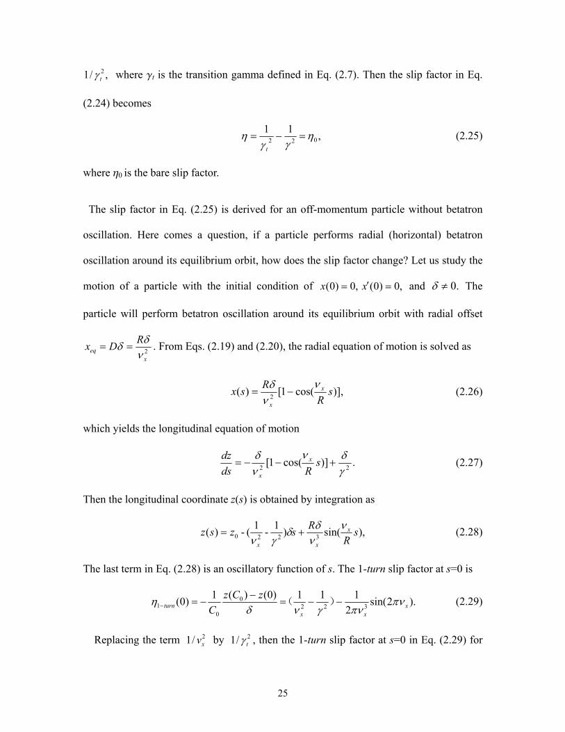
The slip factor in Eq. (2.25) is derived for an off-momentum particle without betatron
oscillation. Here comes a question, if a particle performs radial (horizontal) betatron
oscillation around its equilibrium orbit, how does the slip factor change? Let us study the
motion of a particle with the initial condition of ,0)0( x ,0)0( x and .0 The
particle will perform betatron oscillation around its equilibrium orbit with radial offset
2x
eq
RDx
. From Eqs. (2.19) and (2.20), the radial equation of motion is solved as
)],cos(1[)(2
sR
Rsx x
x
(2.26)
which yields the longitudinal equation of motion
.)]cos(1[22
sRds
dz x
x
(2.27)
Then the longitudinal coordinate z(s) is obtained by integration as
),sin()1
-1
(-)(3220 s
R
Rszsz x
xx
(2.28)
The last term in Eq. (2.28) is an oscillatory function of s. The 1-turn slip factor at s=0 is
).2sin(2
111)0()(1)0(
3220
01 x
xxturn
zCz
C
)( (2.29)
Replacing the term 2/1 xv by 2/1 t , then the 1-turn slip factor at s=0 in Eq. (2.29) for

26
the isochronous ring becomes
).2sin(2
111)0(
3221 xxt
turn
)( (2.30)
The comparison between Eqs. (2.25) and (2.30) indicates that, for an off-momentum
particle performing betatron oscillation around its equilibrium orbit, there is an extra term
)2sin(2
13 xx
in the slip factor. A similar extra term also appears in the 2D dispersion
relation Eq. (4.41) derived in Chapter 4. For the hard-edge model of SIR lattice, the two
terms in Eq. (2.30) are
,011
022
t
and ,083.0-)2sin(2
1-
3x
x
(2.31)
respectively. Then the total slip factor taking into account betatron oscillation effect
becomes negative (below transition). Note that in the conventional definitions of the
momentum compaction factor a and slip factor h, the effects of betatron oscillation are all
neglected. For conventional circular accelerators whose working points are far from
transition, the extra term in the new slip factor can be neglected. While in the isochronous
ring, due to smallness of the bare slip factor h0, this extra term should be taken into
account in the instability analysis. The above discussions show that the betatron
oscillation may destroy the isochronism.
Assume an on-momentum particle coasts along the design trajectory of SIR with
.0)(0)(0)( ssxsx ,, The particle may maintain its isochronous motion for ever
if there are no external perturbing forces. At a given position s1, for some reasons (e.g.,
LSC field, RF electric field), the particle receives a sudden longitudinal kick, so that x(s1)
and x£(s1) are not changed but .0)( 1 s Then according to the above analysis, the
partic
We
isoch
devia
Ap
mode
2.7 N
Figuris rep
As
bunch
densi
densi
densi
the tr
energ
self-f
transi
cle will perfo
e can see tha
hronous moti
ation satisfy
ppendix A p
el) using the
Negative m
re 2.4: Mechproduced fro
sume at a gi
h circulating
ity variation
ity peak regi
ity bump suc
railing side o
gy. The on-m
force and ke
ition, the hi
orm betatron
at, even if in
ion. Only tho
the closed o
provides mor
standard ma
mass instab
hanism of nem Ref. [8]).
iven time, th
g in an acce
ns will prod
ion to the de
ch as P2 will
of the densi
momentum r
eeps a const
gher energy
n oscillation
n an ideal iso
ose particles
rbit conditio
re studies on
atrix formali
bility (mic
egative mass
here are sma
lerator abov
uce a self-f
ensity valley
see a pushin
ity bump suc
reference pa
tant energy.
y particle lik
27
and lose its
ochronous ri
s whose radi
on can maint
n the beam
ism.
crowave in
s instability
all longitudi
ve transition
field (or spa
y region. The
ng force F an
ch as P1 wil
article locate
The discuss
ke P2 has a
isochronism
ing, not all t
ial offset, rad
tain the isoch
optics of th
nstability)
or microwa
inal charge d
as shown in
ace charge f
e particles o
nd gain ener
ll see a pull
ed right at th
sion in Sect
lower revol
m.
the particles
dial slope an
hronous mot
he SIR lattic
)
ave instabilit
density pertu
n Figure 2.4
field) direct
on the forwa
rgy, while th
ling self-forc
he density p
t. 2.5 tells u
lution freque
s can keep th
nd momentum
tion.
ce (hard-edg
ty (The figur
urbations in
4. The charg
ting from th
ard side of th
he particles o
ce F and los
eak sees zer
us that, abov
ency than th
he
m
ge
re
a
ge
he
he
on
se
ro
ve
he
28
on-momentum reference particle, while the lower energy particle like P1 has a higher
revolution frequency than the on-momentum reference particle. This may result in an
enhancement of the azimuthal density modulation amplitude. In beam instability analysis,
this self-bunching phenomenon is usually termed the negative mass instability. The term
comes from the illusion that the particles seem to move in the opposite directions from
the self-force or space charge force exerting on them. Usually the space–charge driven
negative mass instability is characterized by density perturbation wavelengths which are
much shorter than the bunch length. For this reason, it is also named microwave
instability in modern literature.
2.8 Microwave instability in the isochronous regime
The microwave instability in the isochronous regime is the main topic of this
dissertation. It demonstrates some unique features that cannot be explained by the
conventional theory of microwave instability. For example, the instability growth rate is
proportional to the unperturbed beam intensity I0 instead of the square root of I0. This
confusing phenomenon is first explained by Pozdeyev in Refs. [14-15]. He pointed out
that, in a circular accelerator, the longitudinal density modulation produces the
longitudinal space charge (LSC) field modulation and the coherent energy modulation
along the beam. In consequence, the local beam centroid wiggling takes place due to
dispersion function as shown in Figure 2.5. The coherent radial space charge field on the
local centroid is proportional to the local centroid offset, which in turn will modify the
dispersion function D, momentum compaction factor a and produce a positive increment
of the coherent slip factor Dhcoh of the local centroid. For a space-charge dominated beam,
Dhcoh
There
transi
to I0.
Figurspace
Po
wiggl
isoch
2.9 L
As
centr
becom
energ
will
h is proportio
efore, the wo
ition where t
re 2.5: Schee charge field
zdeyev’s th
ling play a
hronous regim
Landau d
discussed i
oid wigglin
mes a quasi
gy (or mome
be a revolu
onal to I0 an
orking point
the microwa
ematic drawids (The figu
eory clearly
a key role
me.
damping
in Sects. 2.6
g may destr
i-isochronou
entum) sprea
ution freque
nd dominate
t of the nomi
ave instabilit
ing of beamre is reprodu
y shows tha
in the me
6 and 2.8, t
roy the isoc
us ring with
ad and emitt
ency spread
29
es over the v
inal isochron
ty may take p
m centroid wuced from R
at the radial
chanism of
the betatron
chronism. T
a non-zero
tance coastin
among the
vanishingly
nous ring tur
place with a
wiggling andRef. [15]).
l-longitudina
f the micro
motion, the
Therefore, an
slip factor.
ng in a quas
e particles.
small bare s
rns out to be
a growth rate
d the associa
al coupling
owave insta
e space cha
n ideal isoc
For a bunc
si-isochrono
The resultin
slip factor h
e raised abov
e proportiona
ated coheren
and centroi
ability in th
arge field an
chronous rin
ch with give
us ring, ther
ng revolutio
h0.
ve
al
nt
id
he
nd
ng
en
re
on
30
frequency spread may tend to counteract and smear out the longitudinal self-bunching,
and then the beam instability will be prevented or suppressed. This mechanism of
instability suppression is termed Landau damping in the literature. Chapter 4 discusses
the Landau damping in the isochronous regime in detail by a 2D dispersion relation.
2.10 Coherent and incoherent motions
The terms of coherent and incoherent are used to describe the properties of a local
beam centroid and a single particle in this dissertation, respectively. The subscripts ‘coh’
and ‘inc’ are added to the corresponding parameters to tell them apart. For example, the
equations of coherent and incoherent radial motions of a SIR beam can be expressed as:
,22
,2
2
2cm
eE
Rx
R
vx
H
cohxcohc
xc
(2.32)
,22
,
2
2
2cm
eE
Rx
R
vx
H
incxincx
(2.33)
where nx is the bare radial betatron tune which is the number of betatron oscillations per
revolution without space charge effects; coh and inc are the coherent and incoherent
fractional momentum deviations, Ex,coh and Ex,inc are the coherent and incoherent radial
space charge fields, respectively.
31
Chapter 3
STUDY OF LONGITUDINAL SPACE CHARGE IMPEDANCES
1
3.1 Introduction
When a charged beam travels along a surrounding metallic vacuum chamber, the space
charge field inside the beam will perturb the beam resulting in beam instability under
some circumstances. For example, the space charge effect plays an important role in the
microwave instability of low energy beam with high intensity near or above transition
[14-16]. The space charge field is also one of the important reasons causing the
microbunching instability for free-electron lasers (FELs) [22]. An accurate calculation of
the LSC fields and impedances is helpful to explain the beam behavior and predict the
growth rates of the beam instability with a good resolution. Both the direct self-fields of
the beam and its image charge fields due to the conducting chamber wall should be taken
into account in the analysis. The image charges may reduce the LSC fields inside the
beam and the associated LSC impedances compared with a beam in free space. This is the
so-called shielding effect of the vacuum chamber.
The LSC field depends on not only the geometric configurations of the cross-sections
of the beam-chamber system, but also the distributions of the beam profiles. Therefore,
the space charge field models which are either exactly the same as or close to the real
beam-chamber system are preferred in beam instability analysis. It is also highly 1 [1] Y. Li, L. Wang, Nuclear Instruments and Methods in Physics Research A 747, 30 (2014).
[2] Y. Li, L. Wang, Nuclear Instruments and Methods in Physics Research A 769, 44 (2015).

32
desirable that the derived space charge fields and impedances are valid at any
perturbation wavelengths. The coasting SIR beam is typically a long bunch with a
roughly round cross-section; the vacuum chamber is roughly rectangular with large
aspect ratio, which can also be simplified as a pair of infinitely large parallel plates (e.g.,
in the simulation code CYCO [12]). Unfortunately, at present, there are no ready-to-use
LSC impedance formulae available for the SIR beam-chamber system in the existing
literature, which satisfy the requirements of both the geometric configuration and the
range of validity in perturbation wavelength. Beam physicists have to use other field
models to approximate the LSC fields of SIR beam instead. For example, Pozdeyev [15]
and Bi [16] use the LSC impedance formulae of a round beam in free space, and a round
beam inside a round chamber to approximate the LSC impedances of SIR beam,
respectively. The accuracies and range of validity of these models sometimes are
questionable. Hence, derivations of more accurate analytical LSC impedance formulae
for the SIR beam-chamber system become the major pursuits of this chapter.
First, this chapter summarizes the existing LSC field models and some popular
methods for analytical derivations of the LSC impedances. Second, this chapter studies
the LSC impedances of a rectangular beam with sinusoidal line charge density
modulations inside a rectangular chamber, and between a pair of parallel plates as a
limiting case. Third, based on the rectangular beam model, this chapter continues to
derive the approximate analytical LSC impedances of a round beam with sinusoidal line
density modulations under planar and rectangular boundary conditions, respectively. The
derived analytical LSC impedances are valid at any perturbation wavelength and are
consistent well with the numerical simulation results.
33
3.2 A summary of the existing LSC field models
Various space charge field models with different cross-sections of the beam and
chamber have been investigated in existing literatures. For example, a round beam in free
space [23-26], a round beam inside a round chamber [16, 24, 25, 27, 28], a round beam
inside an elliptic chamber [29], a uniformly charged line between two parallel plates [30],
a uniformly charged round beam between two parallel plates [31], a uniformly charged
round beam inside a rectangular chamber [32], a rectangular beam inside a rectangular
chamber [33-34], a rectangular beam between parallel plates [35], a single particle
between parallel plates [36], a line charge inside rectangular chamber and between
parallel plates [37], a vertical ribbon beam between parallel plates [38], etc.
The above-mentioned models are either not for a round beam, or/and not for a
rectangular chamber (or between parallel plates), or/and not valid at any perturbation
wavelengths. To our knowledge, at present, there are no analytical LSC impedance
formulae available in modern publications for a round beam inside a straight rectangular
chamber (or between parallel plates) which are valid in the entire wavelength spectrum.
3.3 Review of analytical methods for derivation of the LSC fields
Some (not all) popular methods are used to calculate the analytical LSC fields.
(a) Faraday’s law and rectangular integration loop [21, 32]. This method is only valid in
the long-wavelength limits. When the charge density modulation wavelength l is small,
the electric fields at the off-axis field points have both normal and skew components with
respect to the beam axis. The three-dimensional (3D) effects of the electric fields become

34
important making this method invalid.
(b) Direct integration methods. Usually the direct integration methods are only applicable
to the field models with simple charge distributions in free space. Some literatures use
this method to calculate the LSC fields assuming the gradient of the charge density d/dz
is independent of the longitudinal coordinate z and is put outside of the integral over z
(e.g., Refs. [21, 35]). In fact, this assumption is invalid for a beam with short-wavelength
density modulations (e.g., (z) = kcos(kz), where k=2p/l). Thus the results are only
valid in the long-wavelength limits too.
(c) Separation of variables. In some special cases, the exact analytical 3D space charge
fields of a beam with sinusoidal longitudinal charge density modulations can be solved by
the method of separation of variables, such as a round beam in free space and inside a
round chamber [16, 23, 27]. The 3D space charge fields solved by this method are exact
and valid in the whole spectrum of perturbation wavelengths. But this method is critical
of the configurations of the cross-sectional geometry of the beam-chamber system. Hence,
it is not applicable to all field models.
(d) Image method. According to the superposition theorem of the electric fields, the space
charge field of a beam is equal to the sum of the direct self-field in free space (open
boundary) and its image fields. If these fields can be calculated separately, it is easy to
obtain the total LSC field and impedance.
3.4 LSC impedances of a rectangular beam inside a rectangular chamber and between parallel plates
By separation of variables technique, this section will derive the LSC impedance for a
field model consisting of a rectangular beam with sinusoidal line charge density
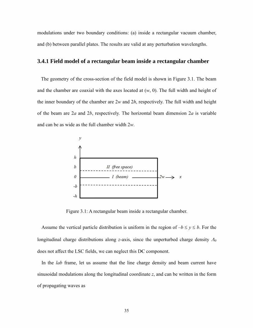
modu
and (b
3.4.1
The
and t
the in
of the
and c
Ass
longi
does
In
sinus
of pro
ulations und
b) between p
1 Field mo
e geometry o
he chamber
nner boundar
e beam are
can be as wid
Fig
sume the ve
tudinal char
not affect th
the lab fram
oidal modul
opagating w
der two boun
parallel plate
odel of a re
of the cross-
are coaxial
ry of the cha
2a and 2b,
de as the full
gure 3.1: A r
rtical particl
rge distribut
he LSC fields
me, let us a
lations along
waves as
ndary condit
es. The resul
ectangular
-section of th
with the axe
amber are 2w
respectively
l chamber w
rectangular b
le distributio
tions along z
s, we can ne
assume that
g the longitud
35
tions: (a) in
lts are valid
r beam ins
he field mod
es located at
w and 2h, re
y. The horizo
width 2w.
beam inside
on is uniform
z-axis, since
eglect this DC
the line cha
dinal coordi
nside a recta
at any pertu
side a rect
del is shown
t (w, 0). The
espectively. T
ontal beam
a rectangula
m in the regi
e the unpert
C componen
arge density
nate z, and c
angular vacu
urbation wav
tangular c
n in Figure 3
e full width
The full wid
dimension 2
ar chamber.
ion of –b y
turbed charg
nt.
y and beam
can be writte
uum chambe
elengths.
chamber
3.1. The beam
and height o
dth and heigh
2a is variabl
y b. For th
ge density
current hav
en in the form
er,
m
of
ht
le
he
0
ve
m
36
)],(exp[),( tkzitz k ,)](exp[),( tkziItzI k (3.1)
respectively, where k and kI are the amplitudes, cI kk , β is the relativistic speed of
the beam, c is the speed of light in free space, ω is the angular frequency of the
perturbations, k is the wave number of the line charge density modulations. In order to
calculate the LSC fields inside the beam in the lab frame, first, we can calculate the
electrostatic potentials and fields in the rest frame of the beam, and then convert them
into the lab frame by Lorentz transformation.
In the rest frame, the line charge density of a beam can be simplified as
),cos()( zkz k (3.2)
where the symbol prime stands for the rest frame.
For general purpose, we assume there are no restrictions for the horizontal beam
distributions within the chamber. If the dependence of the perturbed volume charge
density ),,( zyx on x£ in the rest frame can be described by a function of G(x£), then
,,0
)(2
)cos(),,(
xG
b
zkzyx
k
.||
.||
hyb
by
(3.3)
where G(x£) satisfies the normalization condition of
,1)(2
0 xdxG
w (3.4)
and the volume charge density correlates with the line charge density
).(),,(2
0
zxdzyxydh
h
w
(3.5)
In order to solve the Poisson equation in the Cartesian coordinate system analytically

37
and conveniently using the method of separation of variables, the normalized horizontal
distribution function G(x£) can be written as a Fourier series. Since the charge must
vanish on the chamber side walls at x£ = 0 and x£ = 2w, we can expand G(x£) to a
sinusoidal series
,)sin(2
1)(
1
n
nn xgw
xG (3.6)
.2w
nn
(3.7)
The dimensionless Fourier coefficient can be calculated by
.)sin()(22
0 w
nn xdxxGg (3.8)
From Eq. (3.3) and Eq. (3.6), the volume charge density in the rest frame can be
expressed as
,0
),sin(4
)cos(),,(
1nnn
k xgbw
zkzyx
.||
,||
hyb
by
(3.9)
3.4.2 Calculation of the space charge potentials and fields
In Region I (charge region) and Region II (charge free region), the electrostatic space
charge potentials ( , , ) and ( , , ) in the rest frame satisfy the Poisson
equation and Laplace equation, respectively. Then we have
,)sin(4
)cos(),,()(
102
2
2
2
2
2
nnn
kI xg
bw
zkzyx
zyx
(3.10)
38
,0),,()(2
2
2
2
2
2
zyx
zyxII (3.11)
where 0 = 8.8510-12 F/m is the permittivity in free space.
The basic components of the solutions to Eq. (3.11) and the homogeneous form of Eq.
(3.10) can be written as
).cos()()( zkyYxXh (3.12)
The possible configurations of the solutions to X(x£) and Y(y£) may have the forms of
)sin(),cos(~)( yxxX nn or their combinations, (3.13)
and
)sinh(),cosh(~)( yvyvyY nn or their combinations, (3.14)
respectively, where
,222 kv nn n=1, 2, 3 …… (3.15)
Considering the boundary conditions (a) £ = 0, = 0 at x£ = 0, 2w; (b) £ = 0, = 0
at y£=≤h, and the potential £(x£, y£, z£) should be even functions of y£, the basic
components of solutions to Eq. (3.11) and the homogeneous form of Eq. (3.10) may have
the following forms:
In region I (charge region): ),cos()cosh()sin(~, zkyvx nnIh (3.16)
In region II (charge free region): ).cos(|)]|(sinh[)sin(~, zkyhvx nnIIh (3.17)
The particular solution to the inhomogeneous Eq. (3.10) can be written as

39
.)sin()cos(),,(1
,
n
nnIi xCzkzyx (3.18)
Plugging Eq. (3.18) into Eq. (3.10) and comparing the coefficients of the like terms of the
two sides gives the coefficients
.4 2
0 n
nkn
vbw
gC
(3.19)
Then in region I (charge region), the field potentials in the rest frame are
.])cosh()[sin()cos(),,(1
,,
n
nnnnIiIhI CyvAxzkzyx (3.20)
In region II (charge free region), the field potentials in the rest frame are
1
|)].|(sinh[)sin()cos(),,(n
nnnII yhvxBzkzyx (3.21)
The boundary conditions between Region I and Region II are: at y£=≤b, = , / ′ = / ′. Then the coefficients and can be determined as
,)cosh(
)](cosh[n
n
nn C
hv
bhvA
.)cosh(
)sinh(n
n
nn C
hv
bvB
(3.22)
Finally, the space charge potentials in the rest frame are
(a) In region I (charge region), 0 |y£| b,
.)cosh()cosh(
)](cosh[1)sin(
4
)cos(),,(
12
0
n
nn
nn
n
nk yvhv
bhvx
v
g
bw
zkzyxI
(3.23)
(b) In region II (charge free region), b<|y£|h,
1
20
|)].|(sinh[)sin()cosh(
)sinh(
4
)cos(),,(
nnn
n
n
n
nk yhvxhv
bv
v
g
bw
zkzyxII
(3.24)
40
For a beam with rectangular cross-section and uniform transverse charge density, the
volume charge density in the rest frame can be expressed as
,0
),cos(4),,( zkabzyx
k
.||,,
.||,
hybawxawx
byawxaw
(3.25)
Comparing Eq. (3.25) with Eq. (3.3) gives G(x£) is equal to 1/2a inside the beam and 0
outside of the beam, respectively. Then can be calculated from Eq. (3.8) as
)sin()sin(2
awa
g nnn
n
(3.26)
inside the beam and 0 outside of the beam, respectively.
According to Eq. (3.23), the LSC field inside the beam in the rest frame can be
calculated as
.)cosh()cosh(
)](cosh[1)sin(
4
)(),,(
),,(1
20
,
nn
n
nn
n
nIIz y
h
bhx
g
bwzd
zd
z
zyxzyxE
(3.27)
According to the theory of relativity, the relations of parameters between the rest
frame and the lab frame are
(a) The longitudinal electric field is invariant, i.e.,
,,, IzIz EE (3.28)
(b) The wave number ,/kk (3.29)
(c) The coordinates ,xx ,yy ),( ctzz (3.30)
(d) The line charge density amplitude
,/kk (3.31)
41
(e) ,2
22222
k
kv nnn (3.32)
(f) ).sin()sin()(
2 tkzk
zkkzd
zd kk
(3.33)
If we choose exponential representation as used in Eq. (3.1), then Eq. (3.33) can also
be expressed as
,),(1)(
2 z
tz
zd
zd
(3.34)
where is the relativistic factor. Then the LSC field in the lab frame becomes
,)cosh()cosh(
)](cosh[1)sin(
4
),(
),,,(1
220
,
n
nn
nn
n
nIz y
h
bhx
g
bwz
tz
tzyxE
(3.35)
where
),sin()sin(2
awa
gg nnn
nn
(3.36)
.2
222222
k
kvv nnnn (3.37)
3.4.3 LSC impedances
The average LSC field over the cross-section of the beam at z and time t is
b
b
aw
aw
IzIz dxtzyxEdyab
tzE ),,,(4
1),( ,,
,)cosh()cosh(
)](cosh[1)sin(
4
),(
122
0
n
nn
nn
n
n yh
bhx
g
bwz
tz
(3.38)

42
where
,2
1)sin(
2
1)sin( n
aw
aw
nn gdxxa
x
(3.39)
).sinh(1
)cosh(2
1)cos( bv
bvdyyv
byv n
b
b nnn
(3.40)
Finally, the average LSC fields in the beam region can be expressed as
,),(
)(4
1),(
20
, z
tzk
bwtzE rectIz
(3.41)
where
.)sinh()cosh(
)](cosh[1
2)(
12
2
nn
nn
n
n
nrect b
hb
bhgk
(3.42)
The sum of the infinite series in Eq. (3.42) can be evaluated by truncating it to a finite
number of terms, as long as the sum converges well.
The average energy loss per turn of a unit charge in a storage ring due to the average
LSC field is
)],(exp[)(),( ||,00, tkziIkZCtzE kscIz (3.43)
where C0 is the circumference of the storage ring, )(||,0 kZ sc is the LSC impedance of the
rectangular beam inside the rectangular chamber. It is easy to obtain from Eqs. (3.1),
(3.41) and (3.43) that the LSC impedance (Ω) is
),(4
)(2
00||,,0 k
bw
kCZikZ rectrectrectrect ,
(3.44)
where Z0 = 377 Ω is the impedance of free space, R is the average radius of the storage
43
ring. If the impedance is evaluated by the LSC fields on the beam axis (w, 0), since in Eq.
(3.35), sin(nx)= sin(n/2), cosh(ny)=1, then rect,rect(k) in Eq. (3.42) should be replaced
by
.)cosh(
)](cosh[1)
2sin()(
12,
n n
n
n
naxisrectrect h
bhngk
(3.45)
For a special case of infinite h, i.e., the rectangular chamber becomes a pair of vertical
parallel plates separated by 2w, since when hض, the limit of )cosh(/)](cosh[ hvbhv nn
approaches )sin()cosh( bvbv nn , the parameter rect,rect(k) in Eq. (3.42) can be simplified
as
.)]sinh()sinh()cosh(
1[2
)(1
2
2
,
nn
n
nn
n
nvpprect b
b
bvbgk
(3.46)
Eqs. (3.44) and (3.46) give the LSC impedances of a rectangular beam between a pair of
vertical parallel plates separated by 2w. In Eq. (3.46), if b is infinite, i.e. a rectangular
beam with infinite height between two vertical parallel plates, since the last part in the
right hand side of Eq. (3.46) becomes zero, then
.2
|)(1
2
2
,
n n
nbvpprect
gk
(3.47)
For a special case of w, i.e., the rectangular chamber becomes a pair of horizontal
parallel plates separated by 2h, if we make exchanges a↔b, w↔h, it is easy to obtain its
impedances from Eqs. (3.44) and (3.46) that
),(4
)( ,200||
,,0 kah
kCZikZ hpprecthpprect
(3.48)
44
,)]sinh()sinh()cosh(
1[2
)(1
,,
,,2
,
2,
,
nhppn
hppn
hppnhppn
hppn
hppnhpprect a
a
avagk
(3.49)
where ,2, h
nhppn
(3.50)
2
22
,2
, k
hppnhppn , n=1, 2, 3 ……, (3.51)
).sin()sin(2
,,,
, bhb
g hppnhppnhppn
hppn
(3.52)
Eqs. (3.48)-(3.52) give the LSC impedances of a rectangular beam between a pair of
horizontal parallel plates separated by 2h. In Eq. (3.49), if a , i.e. a rectangular beam
with infinite width between two horizontal parallel plates, since the limit of
[cosh(vn,hppa)-sinh(vn,hppa)]sinh(vn,hpp a)/vn,hppa 0, then
.2
|)(1
2,
2,
,
n hppn
hppnahpprect
gk
(3.53)
3.4.4 Case studies of the LSC impedances
In this subsection, we will calculate the LSC impedances of SIR beam by both
analytical formulae and numerical method.
Lanfa Wang of Stanford Linear Accelerator Center (SLAC) developed a simulation
code that can solve the Poisson equation numerically based on the Finite Element Method
(FEM) [39]. The code can be used to calculate the space charge potentials, fields and
impedances of the beam-chamber system with any configurations of the charge
distributions and boundary shapes. In the rest frame, assume the harmonic volume charge
density can be written as product of the transverse and longitudinal components
45
zkikeyxzyxzyx
),()(),(),,( , (3.54)
where .1),( ydxdyx Similarly, the potential due to the harmonic charge density
is written as
zkieyxzyx ),(),,( . (3.55)
The Poisson equation with Eqs. (3.54) and (3.55) becomes
,),(
)(0
22
yx
k k
(3.56)
where 22222 // yx and 0 on the metal boundary. The potentials given
by Eq. (3.56) with arbitrary beam and chamber shapes can be solved using the FEM. The
whole domain is first divided into many small element regions (finite element). For each
element, the strong form of the Poisson equation Eq. (3.56) can be rewritten as the FEM
equation
,2 QBM k (3.57)
where
ydxdy
N
y
N
x
N
x
NM
eS
jijieij
, (3.58)
eS
jiei dydxNNB '' , (3.59)
0ie
i
qQ . (3.60)
Here N(x£, y£) is called the shape function in FEM, by which the potentials at a field point
P(x£, y£) within an element can be interpolated by the potentials of its neighboring nodes.
N(x£, y£) is related to the coordinates of the field point P(x£, y£) and the nodes of the
46
element region. M is the stiffness matrix with matrix element ejiM , , i and j are the node
indices of the finite element, Se is the integration boundary of the finite element, qi is the
charge at the node i, which is proportional to the harmonic line charge density amplitude Λ . The of Eq. (3.57) at all nodes satisfying equations Eqs. (3.57)-(3.60) and the
boundary condition = 0 on the chamber wall can be solved numerically. Then the
total potentials in the rest frame can be calculated from Eq. (3.55), the corresponding
LSC fields and impedances in the lab frame can be calculated using the similar
procedures in Sect. 3.4.3.
Now we can use the rectangular beam and chamber model to estimate the LSC
impedances of the coasting beam in the Small Isochronous Ring (SIR) at Michigan
State University (MSU) [12]. The ring circumference is C0 = 6.58 m, the kinetic energy of
the beam is Ek=20 keV ( 0.0046, 1.0), the cross-section of the vacuum chamber is
rectangular with w=5.7 cm, h=2.4 cm, the real beam is approximately round with radius
r0 =0.5 cm. We can use a square beam model with a=b=r0=0.5 cm to mimic the round
beam.
Figure 3.2 shows the comparisons of the on-axis and average LSC impedances of SIR
beam between the theoretical calculations and numerical simulations using a square beam
model. We can see that the theoretical and simulated impedances match quite well. Note
that the on-axis LSC impedances are higher than the averaged ones. The former may
overestimate the LSC effects. For this reason, we only plot the average LSC impedances
in Figures 3.3-3.9.
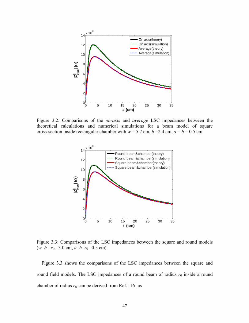
47
Figure 3.2: Comparisons of the on-axis and average LSC impedances between the theoretical calculations and numerical simulations for a beam model of square cross-section inside rectangular chamber with w = 5.7 cm, h =2.4 cm, a = b = 0.5 cm.
Figure 3.3: Comparisons of the LSC impedances between the square and round models (w=h =rw =3.0 cm, a=b=r0 =0.5 cm).
Figure 3.3 shows the comparisons of the LSC impedances between the square and
round field models. The LSC impedances of a round beam of radius r0 inside a round
chamber of radius rw can be derived from Ref. [16] as
0 5 10 15 20 25 30 350
2
4
6
8
10
12
14x 10
6
(cm)
|Z|| 0,
sc| (
)
On axis(theory)On axis(simulation)Average(theory)Average(simulation)
0 5 10 15 20 25 30 350
2
4
6
8
10
12
14x 10
6
(cm)
|Z|| 0
,sc| (
)
Round beam&chamber(theory)Round beam&chamber(simulation)Square beam&chamber(theory)Square beam&chamber(simulation)
48
),()( ,00||
,,0 kkCZ
ikZ roundroundroundround
(3.61)
where )],()()()([)(
)(
)(
1)( 010001
00
02
0, rkIrkKrkIrkK
rkIrk
rkI
rkk ww
wroundround
(3.62)
I0(x), I1(x), K0(x), and K1(x) are the modified Bessel functions, /kk and
.)(2
)(1
)(0
01
0 0
2
020
0
0
rk
rkIrdrrkId
rrkI
r
(3.63)
The parameters used in the calculations are w=h=rw =3.0 cm, a=b=r0 =0.5 cm. We can
observe that the model with square beam and chamber shapes has lower LSC impedances
compared with the round ones. At large perturbation wavelengths, the impedances of the
two field models are close to each other.
Figure 3.4: Simulated LSC impedances of the square and round beam models in a square chamber (w = h =3.0 cm, a = b = r0 = 0.5 cm), respectively.
0 5 10 15 20 25 30 350
2
4
6
8
10
12x 10
6
(cm)
|Z|| 0
,sc| (
)
Round beam inside square chamberSquare beam inside square chamber
49
Figure 3.4 shows the simulated LSC impedances of the square and round H2+ beam of
20 keV inside a same square chamber. The parameters used in the calculations are w=h
=3.0 cm, a=b=r0 =0.5 cm. We can observe that the square beam has relatively lower LSC
impedances than the round beam. The difference of impedances is caused by the different
beam shapes. At large perturbation wavelengths, the LSC impedances of the two field
models are close to each other.
Figure 3.5: Simulated LSC impedances of a round beam inside square and round chambers (w = h = rw = 3.0 cm, r0 = 0.5 cm), respectively.
Figure 3.5 shows the simulated LSC impedances of a round beam of 20 keV inside
the round and square chambers, respectively. The parameters used in the calculations are
w=h=rw=3.0 cm, r0 =0.5 cm. We can observe that the two curves are close to each other,
and the square chamber model has relatively higher LSC impedances than the round
chamber model. The reason for this tiny difference is that the four corners of the square
chamber are relatively farther away from the beam axis compared with a round chamber
inscribing the square chamber, thus the shielding effects of the square chamber due to
0 5 10 15 20 25 30 350
2
4
6
8
10
12x 10
6
(cm)
|Z|| 0,
sc| (
)
Round beam inside square chamberRound beam inside round chamber
50
image charges are weaker, and therefore the LSC field becomes stronger. At large
perturbation wavelengths, the impedances of the two field models are close to each other.
Figures 3.3-3.5 show that the lower impedances of the rectangular beam and chamber
model in Figure 3.3 mainly originate from the different beam shapes rather than the
chamber shapes.
Figure 3.6: LSC impedances of rectangular beam model with different half widths a inside a rectangular chamber (w = 5.7 cm, h = 2.4 cm, a is variable, b = 0.5 cm).
Figure 3.6 shows the calculated LSC impedances of four perturbation wavelengths for a
20 keV beam model with rectangular cross-section inside the rectangular chamber
of SIR. The parameters used in the calculations are w = 5.7 cm, h = 2.4 cm, b = 0.5 cm,
the half beam width a is variable. We can see the LSC impedances decrease with beam
width 2a for a fixed beam height 2b.
Figure 3.7 shows the calculated LSC impedances of four perturbation wavelengths for
a 20 keV beam model with rectangular cross-section inside a rectangular chamber of
SIR. The parameters used in the calculations are w = 5.7 cm, h = 2.4 cm, a = 0.5 cm, the
0 1 2 3 4 5 60
2
4
6
8
10
12
14x 10
6
a (cm)
|Z|| 0
,sc| (
)
1 = 1.0 cm
2 = 2.0 cm
3 = 5.0 cm
4 = 10.0 cm
51
half beam height b is variable. We can see the LSC impedances decrease with beam
height 2b for a fixed beam width 2a.
Figure 3.7: LSC impedances of a rectangular beam model with different half heights b inside rectangular chamber (w = 5.7 cm, h = 2.4 cm, a = 0.5 cm, b is variable).
Figure 3.8: LSC impedances of square beam model inside rectangular chamber (w = 5.7 cm, h is variable, a = b = 0.5 cm).
0 0.5 1 1.5 2 2.50
2
4
6
8
10
12
14x 10
6
b (cm)
|Z|| 0
,sc| (
)
1 = 1.0 cm
2 = 2.0 cm
3 = 5.0 cm
4 = 10.0 cm
0 5 10 15 20 25 30 350
2
4
6
8
10x 10
6
(cm)
|Z|| 0,
sc| (
)
h = 1.5 cm h = 2.0 cm h = 2.4 cm h = 5.0 cm h = Inf.
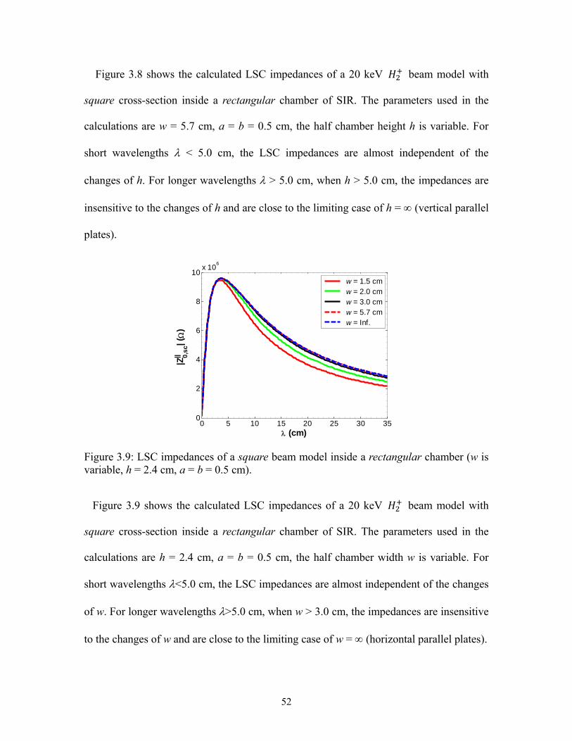
52
Figure 3.8 shows the calculated LSC impedances of a 20 keV beam model with
square cross-section inside a rectangular chamber of SIR. The parameters used in the
calculations are w = 5.7 cm, a = b = 0.5 cm, the half chamber height h is variable. For
short wavelengths < 5.0 cm, the LSC impedances are almost independent of the
changes of h. For longer wavelengths > 5.0 cm, when h > 5.0 cm, the impedances are
insensitive to the changes of h and are close to the limiting case of h = (vertical parallel
plates).
Figure 3.9: LSC impedances of a square beam model inside a rectangular chamber (w is variable, h = 2.4 cm, a = b = 0.5 cm).
Figure 3.9 shows the calculated LSC impedances of a 20 keV beam model with
square cross-section inside a rectangular chamber of SIR. The parameters used in the
calculations are h = 2.4 cm, a = b = 0.5 cm, the half chamber width w is variable. For
short wavelengths <5.0 cm, the LSC impedances are almost independent of the changes
of w. For longer wavelengths >5.0 cm, when w > 3.0 cm, the impedances are insensitive
to the changes of w and are close to the limiting case of w = (horizontal parallel plates).
0 5 10 15 20 25 30 350
2
4
6
8
10x 10
6
(cm)
|Z|| 0
,sc| (
)
w = 1.5 cm w = 2.0 cm w = 3.0 cm w = 5.7 cm w = Inf.
53
3.4.5 Conclusions for the rectangular beam model
We introduced a 3D space charge field model of rectangular cross-section to calculate
the perturbed potentials, fields and the associated LSC impedances. The calculated LSC
impedances are consistent well with the numerical simulation results. A rectangular beam
shape with a=b=r0 may help to reduce the LSC impedances compared with the
conventional round beam with radius r0. This result is consistent with Ref. [35] in which
a planar geometry was investigated. For fixed b(or a), when a(or b) increases, the LSC
impedance will decrease. The LSC impedances of a rectangular beam inside a pair of
infinitely large parallel plates are also derived in this paper. Theoretical calculations
demonstrate that, when the transverse chamber dimensions are approximately more than
five times of the transverse beam dimensions, the rectangular chamber of the Small
Isochronous Ring (SIR) can be approximated by a pair of parallel plates. This result
validates the simplified boundary model of parallel plates used in the Particle-In-Cell
(PIC) simulation code CYCO to simulate the rectangular chamber of SIR [12].
3.5 LSC impedances of a round beam inside a rectangular chamber and between parallel plates
This section presents the approximate analytical solutions to the LSC impedances of a
round beam with uniform transverse distribution and sinusoidal line density modulations
under two boundary conditions: (a) between parallel plates (b) inside a rectangular
chamber, respectively. Since the transverse dimensions of almost all the beam chambers
are much larger than the transverse beam size, the image charge fields of a round beam
can be approximated by those of a line charge. Then the approximate LSC fields and
54
impedances of the two models in discussion can be calculated by image method.
In order to obtain the approximate analytical LSC impedances of a round beam with
planar and rectangular boundary conditions, first, we need to know the LSC fields Ez of
the following four component field models:
(a) A round beam in free space, Ez,round,fs.
(b) A line charge in free space, Ez,line,fs.
(c) A line charge between two parallel plates, Ez,line,pp.
(d) A line charge inside a rectangular chamber Ez,line,rect.
For a round beam between a pair of parallel plates, when the separation between the
plates is much larger than the beam diameter, its image LSC fields can be approximated
by those of a line charge between the parallel plates as imagepplinez
imagepproundz EE ,,,, fslinezpplinez EE ,,,, ,
its total LSC fields are approximately equal to imagepproundzfsroundzpproundz EEE ,,,,,,
imagepplinezfsroundz EE ,,,, fslinezpplinezfsroundz EEE ,,,,,, ; similarly, for a round beam inside a
rectangular chamber, when the full chamber height is much larger than the beam
diameter, its image LSC fields imagerectroundzE ,, and total LSC fields rectroundzE ,, can be
approximated as imagerectroundzE ,, fslinezrectlinez EE ,,,, and rectroundzE ,, fslinezrectlinezfsroundz EEE ,,,,,,
respectively. Next, we will derive the LSC fields of the four component field models
listed in (a)-(d).
55
3.5.1 A round beam in free space
In the lab frame, assume there is an infinitely long round beam of radius r0 with
sinusoidal line density L and beam intensity modulations I of
)],(exp[),( tkzitz k and )],(exp[),( tkziItzI k
(3.64)
respectively. According to Ref. [26], its LSC field in the lab frame is
)].()(1[),(1
),,( 00122200
,, rkIrkKz
tz
krtzrE fsroundz
(3.65)
where 0 = 8.8510-12 F m-1 is the permittivity in free space, = / , is the relativistic
factor, I0(x) and K1(x) are the modified Bessel functions of the first and second kinds,
respectively.
3.5.2 A line charge in free space
In the lab frame, assume there is an infinitely long line charge in free space with
sinusoidal line charge density and beam intensity modulations described in Eq. (3.64).
First, we can calculate its potentials and fields in the rest frame of the beam, and then
convert them into the lab frame by Lorentz transformation. In the rest frame of the beam,
the line charge density is
),cos()( zkz k
(3.66)
where the parameters with primes stand for those in the rest frame. The electrostatic
potentials can be calculated easily in cylindrical coordinate system by direct integration
as
56
).(2
)(
])[(
)cos(
4),( 0
02
1220
, rkKz
zd
rzz
zkzr k
fsline
(3.67)
The LSC field in the rest frame is
).()(
2
1),( 0
0,, rkK
zd
zdzrE fslinez
(3.68)
In the lab frame, according to the theory of relativity, we have
,zz EE (3.69)
,rr (3.70)
),( ctzz (3.71)
/kk , (3.72)
,kk
k (3.73)
).sin()sin('
)(2
tkzk
zkkdz
zd kk
(3.74)
If we choose exponential representation as used in Eq. (3.64), then Eq. (3.74) can also be
expressed as
.),(1)(
2 z
tz
zd
zd
(3.75)
From Eqs. (3.68)-(3.75), the LSC fields in the lab frame become
).(),(
2
1),,( 02
0,, rkK
z
tztzrE fslinez
(3.76)
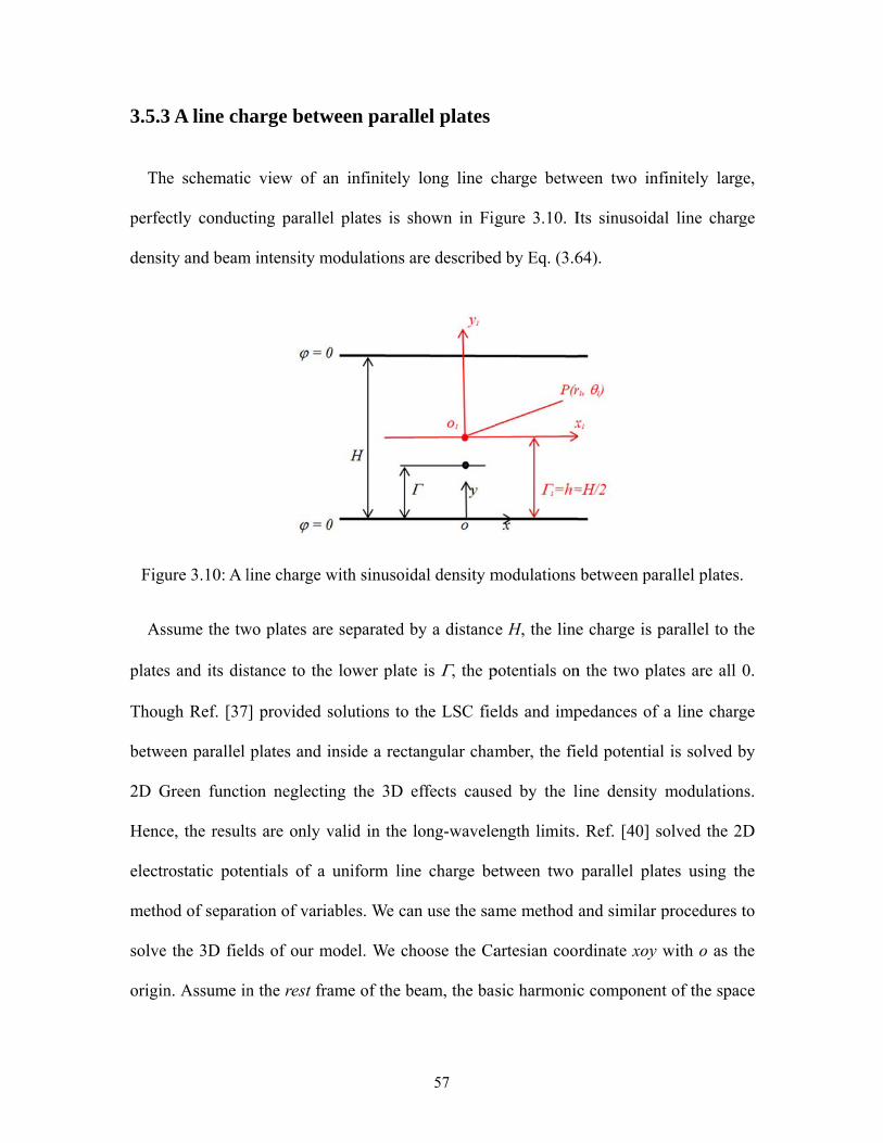
3.5.3
Th
perfe
densi
Figu
As
plates
Thou
betwe
2D G
Henc
electr
metho
solve
origin
3 A line ch
he schematic
ctly conduc
ity and beam
ure 3.10: A l
ssume the tw
s and its dis
ugh Ref. [37
een parallel
Green functi
ce, the result
rostatic pote
od of separa
e the 3D fiel
n. Assume in
harge betw
c view of a
ting parallel
m intensity m
line charge w
wo plates are
stance to the
] provided s
plates and i
ion neglectin
ts are only v
entials of a
ation of varia
lds of our m
n the rest fra
ween paral
n infinitely
l plates is s
modulations a
with sinusoid
e separated b
e lower plate
solutions to
inside a rect
ng the 3D e
valid in the
uniform lin
ables. We ca
model. We ch
ame of the b
57
llel plates
long line c
shown in Fig
are described
dal density m
by a distance
e is , the p
the LSC fie
angular cham
effects caus
long-wavele
ne charge be
an use the sam
hoose the Ca
beam, the bas
charge betw
gure 3.10. I
d by Eq. (3.6
modulations
e H, the line
potentials on
elds and imp
mber, the fie
ed by the l
ength limits.
etween two
ame method
artesian coo
sic harmonic
ween two inf
Its sinusoida
64).
between par
e charge is p
n the two pla
pedances of
eld potential
ine density
. Ref. [40] s
parallel pla
and similar p
rdinate xoy
c componen
finitely larg
al line charg
rallel plates.
parallel to th
ates are all 0
a line charg
l is solved b
modulation
solved the 2D
ates using th
procedures t
with o as th
nt of the spac
e,
ge
he
0.
ge
by
ns.
D
he
to
he
ce
58
charge potential can be written in the form
),cos()()(),,(, zkyYxXzyxppline (3.77)
which satisfies the Laplace equation
.02
,2
2
,2
2
,2
zyxpplinepplineppline
(3.78)
Plugging Eq. (3.77) into Eq. (3.78) results in
.11 2
2
2
2
2
kyd
Yd
Yxd
Xd
X
(3.79)
Considering the boundary conditions £line,pp (y £ = 0) = £
line,pp (y £= H) = £line,pp (x
£= )
= 0, we can choose
,222
21
kxd
Xd
X ,
1 22
2
yd
Yd
Y (3.80)
where > 0. Then the solutions to Eq. (3.80) can be written as
,)(2222
21xkxk eAeAxX
(3.81)
).cos()sin()( 21 yByByY (3.82)
The boundary conditions ppline, (y£=0)= ppline, (y£=H)=0 give 2B =0,=n/H, then Y(y£)sin(n
y£/H). Because at x£=0, there is a line charge which produces singularity, we should
calculate the electrostatic potentials ,, ppline for x£ > 0 and ,, ppline for x£ < 0 separately.
59
In Eq. (3.81), when x£ +, ,, ppline 0, then the coefficient 1A =0; when x£ -,
,, ppline 0, then the coefficient 2A =0. The solutions of X can be written as
xkeAxX
22
)( (3.83)
where‘+ ’and ‘–’stand for x>0 and x<0, respectively.
The potentials including all harmonic components can be expressed as
),cos()sin(
22
1,, zky
H
neC
xH
nk
nnppline
(3.84)
where nC and -nC are the coefficients to be determined by the boundary conditions for
x>0 and x<0, respectively. At x£=0, y£, ,, ppline = ,, ppline which gives nC = nC = nC .
If the line charge is rewritten in the form of surface charge density
),()( yz (3.85)
where (x) is the Dirac Delta function, then on the plane x£ = 0, the boundary condition
D2n£– D1n
£ = £ gives
).()cos(|)( 0,,pp,-line,
0
yzkxx kx
ppline
(3.86)
Eqs. (3.84) and (3.86) give
).()sin(2
01
22
yyH
n
H
nkC k
nn
(3.87)
Multiplying the two sides of Eq. (3.87) by sin(ny£/H) and integrating y£ from 0 to H

60
gives the coefficient
).sin(2
20
H
n
H
nkH
C kn
(3.88)
Then the potentials in Eq. (3.84) can be expressed as
.)sin()sin(1)(
),,(1
||
220
,
22
n
xH
nk
ppline yH
ne
H
n
H
nk
H
zzyx
(3.89)
Let’s consider a special case of =1=h=H/2, i.e., the line charge is on the median
plane of the two plates as shown in Figure 3.10, if we choose a new coordinate system
x1o1y1 with o1 as the origin (see Figure 3.10), according to x£ = , y£= +h, the potentials
in the rest frame of the beam become
.)](2
sin[)2
sin(
2
1
2
)(),,(
11
||2
220
11,
1
22
n
xh
nk
ppline hyh
ne
n
h
nk
h
zzyx
(3.90)
If we use cylindrical coordinate system, = r£cos(£), =r£sin(£), Eq. (3.90) becomes
)].)sin((2
sin[)2
sin(
2
1
2
)(),,(
|)cos(|2
12
20,
22
hrh
ne
n
h
nk
h
zzr
rh
nk
nppline
(3.91)
The LSC field in the rest frame is
61
)].)sin((2
sin[)2
sin(
2
1)(
2
1),,(
)||cos(2
12
20,,'
22
hrh
ne
n
h
nk
zd
zd
hzrE
rh
nk
npplinez
(3.92)
Using the Lorentz transformation of Eqs. (3.69) - (3.75), and £=, the LSC field in the
lab frame becomes
)].)sin((2
sin[)2
sin(
2
1),(
2
1),,,(
|)cos(|2
12
2
20
,,
22
hrh
ne
n
h
nk
z
tz
htzrE
rh
nk
npplinez
(3.93)
3.5.4 A line charge inside a rectangular chamber
In the lab frame, assume there is an infinitely long line charge centered inside a
rectangular chamber, the sinusoidal line charge density and beam intensity modulations
are described in Eq. (3.64). The full chamber width and height are W=2w and H=2h,
respectively. Sect. 3.4.2 derives the potential of an infinitely long beam with rectangular
cross-section and uniform transverse charge density inside a rectangular chamber. In the
rest frame of beam, in the charge-free region inside the chamber (b|y£|h), the potentials
are
,|)]|(sinh[)](sin[)cosh(
)sinh(
4
)cos(),,(
.12
0,,
n
nnn
n
n
nkrectrectII yhvwx
hv
bv
v
g
bw
zkzyx
(3.94)
where ,)sin()sin(2
awa
gg nnn
nn
(3.95)
and n=n/2w, n£2=n
2+k£2, n=1, 2, 3,…. In the limiting case of a=b=0, the rectangular
62
beam shrinks to a line charge. Because a=0, gn£=gn=2sin(nw) and b=0, sinh(n
£ b)/b=n
£,
then Eq. (3.94) becomes
.10,, |)].|(sinh[)](sin[
)cosh(
)sin(
2
)(),,(
nnn
nn
nrectlineII yhvwx
hv
w
w
zzyx
(3.96)
Using the Lorentz transformation of x£= x, y£ = y, and Eqs. (3.69), (3.71)-(3.75), the LSC
field in the lab frame becomes
.1
20
,, |)]|(sinh[)](sin[)cosh(
)sin(),(
2
1),,,(
nnn
nn
nrectlinez yhvwx
hv
w
z
tz
wtzyxE ,
(3.97)
where ./ 2222222 kkvv nnnn
3.5.5 Approximate LSC impedances of a round beam between parallel plates and inside a rectangular chamber
The average longitudinal wake potential (or energy loss per turn of a unit charge) in a
circular accelerator due to the LSC field is
)],(exp[)(),(V ||00 tkziIkZCEtz kz (3.98)
where <Ez> is the LSC field averaged over the cross-section of the round beam and can
be calculated using the formula
63
.),(1
),(0
0
2
020
r
rdrrfdr
rf
(3.99)
(a) For a round beam midway between parallel plates, the average LSC impedance can
be calculated by Eqs. (3.65), (3.76), (3.92), and (3.98) with pproundzz EE ,,
fslinezpplinezfsroundz EEE ,,,,,, as
,])(2
1)[()(2
)(0
0101
0
00,
00||,,0 rk
rkIrkK
r
CZik
h
CZikZ pplineppround
(3.100)
where
.)])sin((2
sin[)2
sin(
21
1)(
1
|)cos(|2
1
2,
2
n
rkhk
n
ppline hrh
ne
n
hk
nk
(3.101)
(b) For a round beam inside and coaxial with a rectangular chamber, the approximate
average LSC impedance can be calculated by Eqs. (3.65), (3.76), (3.97), and (3.98)
with fslinezrectlinezfsroundzrectroundzz EEEEE ,,,,,,,, as
,])(2
1)[()(2
)(0
0101
0
00,
00||,,0 rk
rkIrkK
r
CZik
w
CZikZ rectlinerectround
(3.102)
where
.1
, .|)])sin(|(sinh[)])cos((sin[)cosh(
)sin()(
nnn
nn
nrectline rhvwr
hv
wkk
(3.103)
In the derivations of Eqs. (3.100) and (3.102), two identities of integrals
64
0
10 )(1)( KdxxxK and
0
10 )()( IdxxxI are used. Note that the first terms on the
right hand side of Eqs. (3.100) and (3.102) are contributed from the average LSC fields
of a line charge midway between parallel plates and inside a rectangular chamber,
respectively; the second terms are contributed from the differences of the average LSC
fields within beam radius r0 between a round beam and a line charge in free space. Eqs.
(3.101) and (3.103) can be evaluated by truncating the infinite series to a finite number of
terms, as long as the sum converges well.
3.5.6 Summary of some LSC impedances formulae
For the purpose of comparisons in Sect. 3.5.7, here we would like to summarize some
LSC impedance formulae in both the long-wavelength and short-wavelength limits,
which are often used in literatures.
3.5.6.1 A round beam inside a round chamber
For a round beam with radius r0 and uniform transverse distribution centered inside a
round chamber with inner chamber wall radius rw, the LSC impedance is repeated here as
.)]()()()([)(
12
)( 0100010
12
0
0||,,0 rkIrkKrkIrkK
rkI
f
rk
RZikZ ww
wroundround
(3.104)
where = for the on-axis impedance [24, 25] and = 2 ( ) for the average
one (see Eqs. (3.61)-(3.63)), respectively.
(a) In the long-wavelength limits
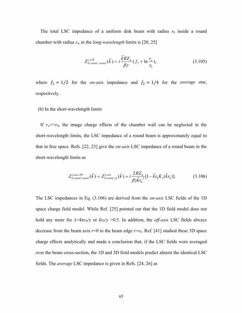
65
The total LSC impedance of a uniform disk beam with radius r0 inside a round
chamber with radius rw in the long-wavelength limits is [20, 25]
),ln()(0
20||,
,,0 r
rf
RZkikZ wLW
roundround
(3.105)
where = 1/2 for the on-axis impedance and = 1/4 for the average one,
respectively.
(b) In the short-wavelength limits
If rw>>r0, the image charge effects of the chamber wall can be neglected in the
short-wavelength limits, the LSC impedance of a round beam is approximately equal to
that in free space. Refs. [22, 23] give the on-axis LSC impedance of a round beam in the
short-wavelength limits as
)].(1[2
)()( 01020
0||,,,0
,||,,,0 rkKrk
rk
RZikZkZ axis
fsroundSWaxis
roundround
(3.106)
The LSC impedances in Eq. (3.106) are derived from the on-axis LSC fields of the 1D
space charge field model. While Ref. [25] pointed out that the 1D field model does not
hold any more for l<4pr0/g or kr0/g >0.5. In addition, the off-axis LSC fields always
decrease from the beam axis r=0 to the beam edge r=r0. Ref. [41] studied these 3D space
charge effects analytically and made a conclusion that, if the LSC fields were averaged
over the beam cross-section, the 1D and 3D field models predict almost the identical LSC
fields. The average LSC impedance is given in Refs. [24, 26] as
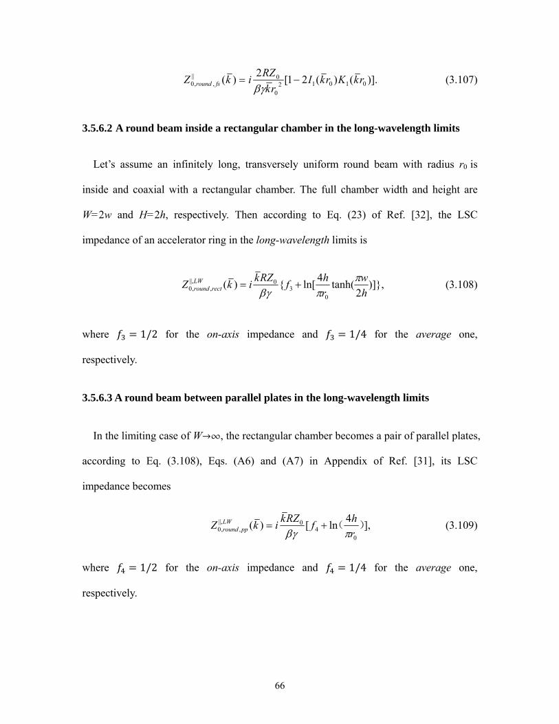
66
)].()(21[2
)( 010120
0||,,0 rkKrkI
rk
RZikZ fsround
(3.107)
3.5.6.2 A round beam inside a rectangular chamber in the long-wavelength limits
Let’s assume an infinitely long, transversely uniform round beam with radius r0 is
inside and coaxial with a rectangular chamber. The full chamber width and height are
W=2w and H=2h, respectively. Then according to Eq. (23) of Ref. [32], the LSC
impedance of an accelerator ring in the long-wavelength limits is
)],2
tanh(4
ln[)(0
30||,
,,0 h
w
r
hf
RZkikZ LW
rectround
(3.108)
where = 1/2 for the on-axis impedance and = 1/4 for the average one,
respectively.
3.5.6.3 A round beam between parallel plates in the long-wavelength limits
In the limiting case of Wض, the rectangular chamber becomes a pair of parallel plates,
according to Eq. (3.108), Eqs. (A6) and (A7) in Appendix of Ref. [31], its LSC
impedance becomes
],4
ln[)(0
40||,
,,0 )(r
hf
RZkikZ LW
ppround (3.109)
where = 1/2 for the on-axis impedance and = 1/4 for the average one,
respectively.
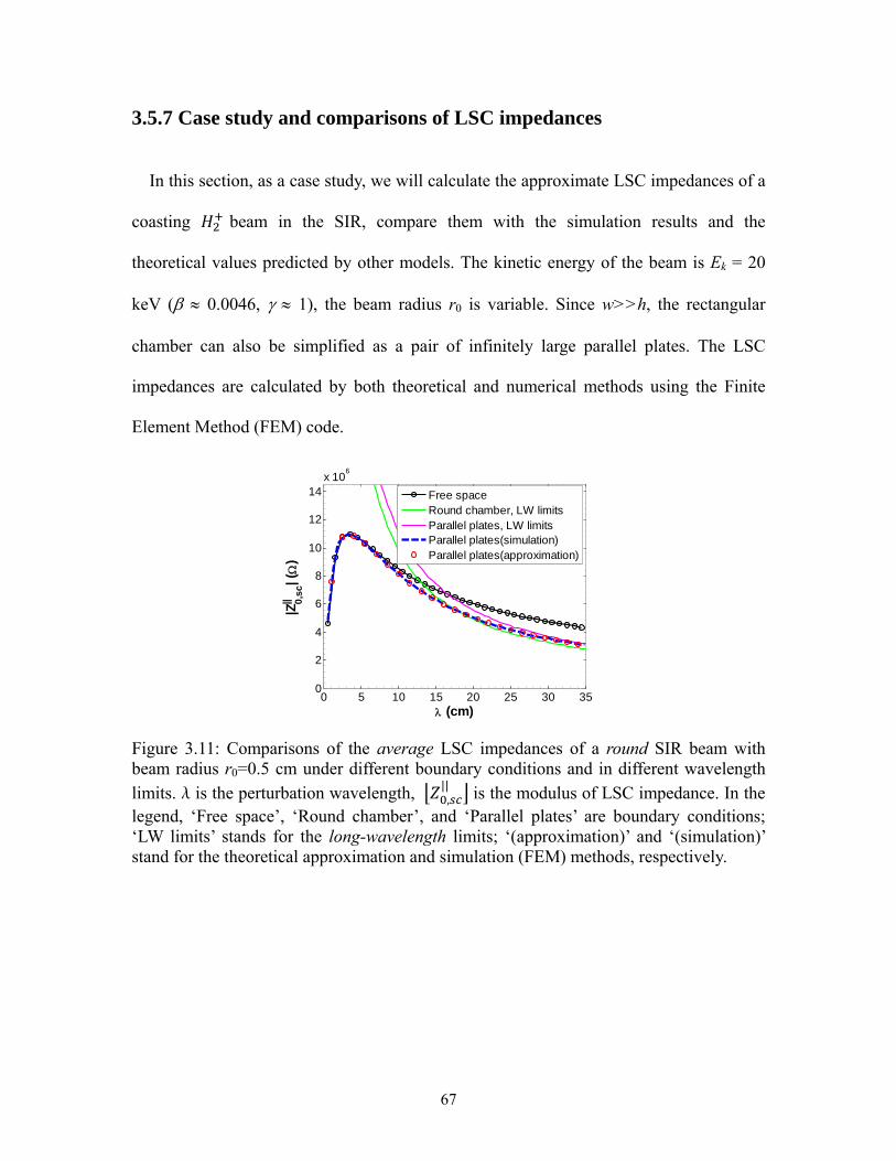
67
3.5.7 Case study and comparisons of LSC impedances
In this section, as a case study, we will calculate the approximate LSC impedances of a
coasting beam in the SIR, compare them with the simulation results and the
theoretical values predicted by other models. The kinetic energy of the beam is Ek = 20
keV ( 0.0046, 1), the beam radius r0 is variable. Since w>>h, the rectangular
chamber can also be simplified as a pair of infinitely large parallel plates. The LSC
impedances are calculated by both theoretical and numerical methods using the Finite
Element Method (FEM) code.
Figure 3.11: Comparisons of the average LSC impedances of a round SIR beam with beam radius r0=0.5 cm under different boundary conditions and in different wavelength limits. l is the perturbation wavelength, ,|| is the modulus of LSC impedance. In the legend, ‘Free space’, ‘Round chamber’, and ‘Parallel plates’ are boundary conditions; ‘LW limits’ stands for the long-wavelength limits; ‘(approximation)’ and ‘(simulation)’ stand for the theoretical approximation and simulation (FEM) methods, respectively.
0 5 10 15 20 25 30 350
2
4
6
8
10
12
14x 10
6
(cm)
|Z|| 0
,sc| (
)
Free spaceRound chamber, LW limitsParallel plates, LW limitsParallel plates(simulation)Parallel plates(approximation)
68
Figure 3.12: Comparisons of the average LSC impedances of a round SIR beam with beam radius r0=1.0 cm under different boundary conditions and in different wavelength limits.
Figure 3.13: Comparisons of the average LSC impedances of a round SIR beam with beam radius r0=1.5 cm under different boundary conditions and in different wavelength limits.
0 5 10 15 20 25 30 350
1
2
3
4
5
6
7
8
9x 10
6
(cm)
|Z|| 0
,sc| (
)
Free spaceRound chamber, LW limitsParallel plates, LW limitsParallel plates(simulation)Parallel plates(approximation)
0 5 10 15 20 25 30 350
1
2
3
4
5x 10
6
(cm)
|Z|| 0
,sc| (
)
Free spaceRound chamber, LW limitsParallel plates, LW limitsParallel plates(simulation)Parallel plates(approximation)
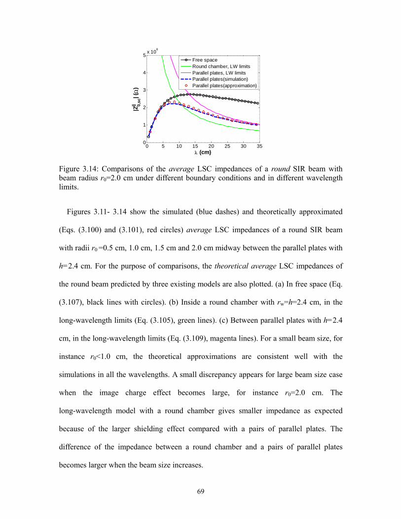
69
Figure 3.14: Comparisons of the average LSC impedances of a round SIR beam with beam radius r0=2.0 cm under different boundary conditions and in different wavelength limits.
Figures 3.11- 3.14 show the simulated (blue dashes) and theoretically approximated
(Eqs. (3.100) and (3.101), red circles) average LSC impedances of a round SIR beam
with radii r0 =0.5 cm, 1.0 cm, 1.5 cm and 2.0 cm midway between the parallel plates with
h=2.4 cm. For the purpose of comparisons, the theoretical average LSC impedances of
the round beam predicted by three existing models are also plotted. (a) In free space (Eq.
(3.107), black lines with circles). (b) Inside a round chamber with rw=h=2.4 cm, in the
long-wavelength limits (Eq. (3.105), green lines). (c) Between parallel plates with h=2.4
cm, in the long-wavelength limits (Eq. (3.109), magenta lines). For a small beam size, for
instance r0<1.0 cm, the theoretical approximations are consistent well with the
simulations in all the wavelengths. A small discrepancy appears for large beam size case
when the image charge effect becomes large, for instance r0=2.0 cm. The
long-wavelength model with a round chamber gives smaller impedance as expected
because of the larger shielding effect compared with a pairs of parallel plates. The
difference of the impedance between a round chamber and a pairs of parallel plates
becomes larger when the beam size increases.
0 5 10 15 20 25 30 350
1
2
3
4
5x 10
6
(cm)
|Z|| 0
,sc| (
)
Free spaceRound chamber, LW limitsParallel plates, LW limitsParallel plates(simulation)Parallel plates(approximation)
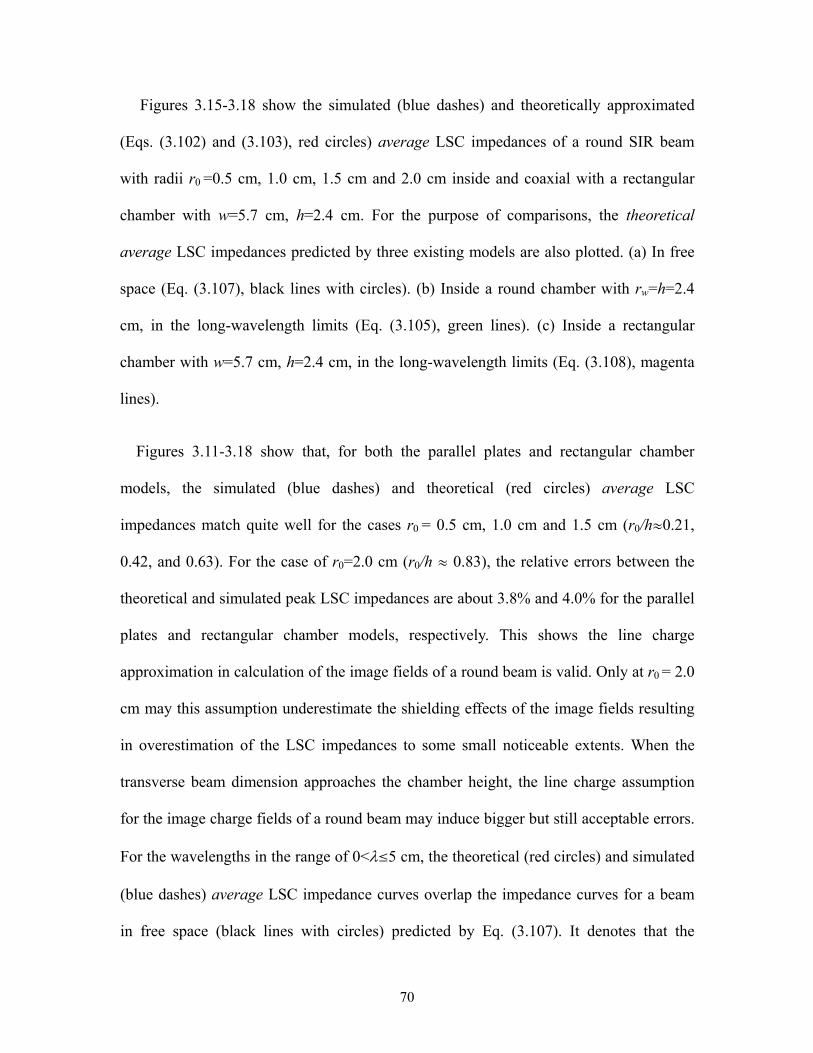
70
Figures 3.15-3.18 show the simulated (blue dashes) and theoretically approximated
(Eqs. (3.102) and (3.103), red circles) average LSC impedances of a round SIR beam
with radii r0 =0.5 cm, 1.0 cm, 1.5 cm and 2.0 cm inside and coaxial with a rectangular
chamber with w=5.7 cm, h=2.4 cm. For the purpose of comparisons, the theoretical
average LSC impedances predicted by three existing models are also plotted. (a) In free
space (Eq. (3.107), black lines with circles). (b) Inside a round chamber with rw=h=2.4
cm, in the long-wavelength limits (Eq. (3.105), green lines). (c) Inside a rectangular
chamber with w=5.7 cm, h=2.4 cm, in the long-wavelength limits (Eq. (3.108), magenta
lines).
Figures 3.11-3.18 show that, for both the parallel plates and rectangular chamber
models, the simulated (blue dashes) and theoretical (red circles) average LSC
impedances match quite well for the cases r0 = 0.5 cm, 1.0 cm and 1.5 cm (r0/hº0.21,
0.42, and 0.63). For the case of r0=2.0 cm (r0/h º 0.83), the relative errors between the
theoretical and simulated peak LSC impedances are about 3.8% and 4.0% for the parallel
plates and rectangular chamber models, respectively. This shows the line charge
approximation in calculation of the image fields of a round beam is valid. Only at r0 = 2.0
cm may this assumption underestimate the shielding effects of the image fields resulting
in overestimation of the LSC impedances to some small noticeable extents. When the
transverse beam dimension approaches the chamber height, the line charge assumption
for the image charge fields of a round beam may induce bigger but still acceptable errors.
For the wavelengths in the range of 0<§5 cm, the theoretical (red circles) and simulated
(blue dashes) average LSC impedance curves overlap the impedance curves for a beam
in free space (black lines with circles) predicted by Eq. (3.107). It denotes that the
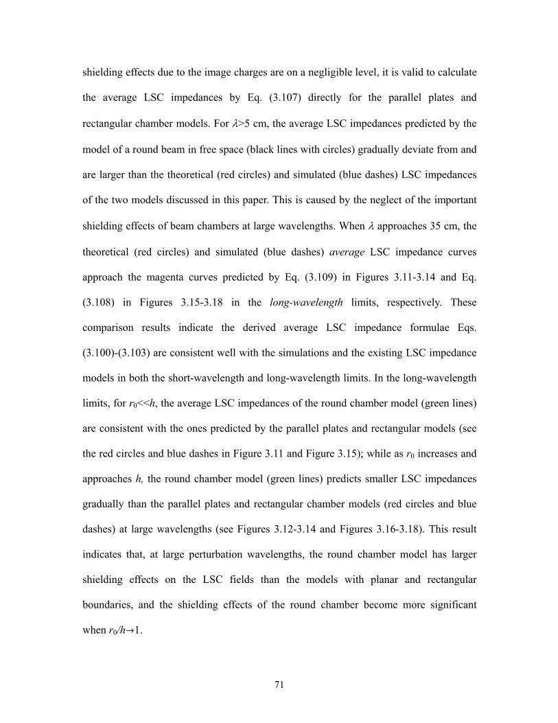
71
shielding effects due to the image charges are on a negligible level, it is valid to calculate
the average LSC impedances by Eq. (3.107) directly for the parallel plates and
rectangular chamber models. For >5 cm, the average LSC impedances predicted by the
model of a round beam in free space (black lines with circles) gradually deviate from and
are larger than the theoretical (red circles) and simulated (blue dashes) LSC impedances
of the two models discussed in this paper. This is caused by the neglect of the important
shielding effects of beam chambers at large wavelengths. When approaches 35 cm, the
theoretical (red circles) and simulated (blue dashes) average LSC impedance curves
approach the magenta curves predicted by Eq. (3.109) in Figures 3.11-3.14 and Eq.
(3.108) in Figures 3.15-3.18 in the long-wavelength limits, respectively. These
comparison results indicate the derived average LSC impedance formulae Eqs.
(3.100)-(3.103) are consistent well with the simulations and the existing LSC impedance
models in both the short-wavelength and long-wavelength limits. In the long-wavelength
limits, for r0<<h, the average LSC impedances of the round chamber model (green lines)
are consistent with the ones predicted by the parallel plates and rectangular models (see
the red circles and blue dashes in Figure 3.11 and Figure 3.15); while as r0 increases and
approaches h, the round chamber model (green lines) predicts smaller LSC impedances
gradually than the parallel plates and rectangular chamber models (red circles and blue
dashes) at large wavelengths (see Figures 3.12-3.14 and Figures 3.16-3.18). This result
indicates that, at large perturbation wavelengths, the round chamber model has larger
shielding effects on the LSC fields than the models with planar and rectangular
boundaries, and the shielding effects of the round chamber become more significant
when r0/hØ1.
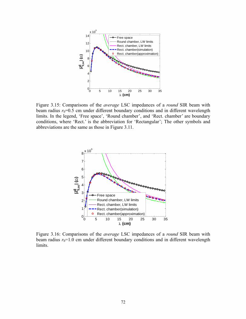
72
Figure 3.15: Comparisons of the average LSC impedances of a round SIR beam with beam radius r0=0.5 cm under different boundary conditions and in different wavelength limits. In the legend, ‘Free space’, ‘Round chamber’, and ‘Rect. chamber’ are boundary conditions, where ‘Rect.’ is the abbreviation for ‘Rectangular’; The other symbols and abbreviations are the same as those in Figure 3.11.
Figure 3.16: Comparisons of the average LSC impedances of a round SIR beam with beam radius r0=1.0 cm under different boundary conditions and in different wavelength limits.
0 5 10 15 20 25 30 350
2
4
6
8
10
12
14x 10
6
(cm)
|Z|| 0
,sc| (
)
Free spaceRound chamber, LW limitsRect. chamber, LW limitsRect. chamber(simulation)Rect. chamber(approximation)
0 5 10 15 20 25 30 350
1
2
3
4
5
6
7
8x 10
6
(cm)
|Z|| 0
,sc| (
)
Free spaceRound chamber, LW limitsRect. chamber, LW limitsRect. chamber(simulation)Rect. chamber(approximation)
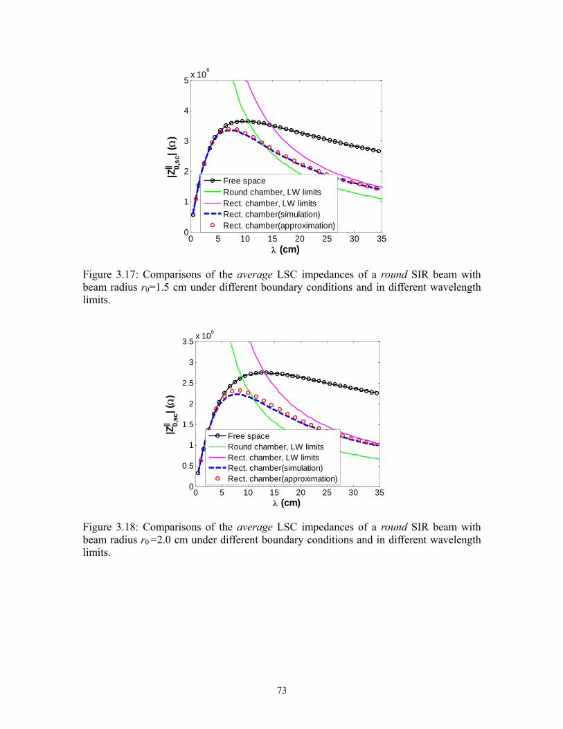
73
Figure 3.17: Comparisons of the average LSC impedances of a round SIR beam with beam radius r0=1.5 cm under different boundary conditions and in different wavelength limits.
Figure 3.18: Comparisons of the average LSC impedances of a round SIR beam with beam radius r0 =2.0 cm under different boundary conditions and in different wavelength limits.
0 5 10 15 20 25 30 350
1
2
3
4
5x 10
6
(cm)
|Z|| 0,
sc| (
)
Free spaceRound chamber, LW limitsRect. chamber, LW limitsRect. chamber(simulation)Rect. chamber(approximation)
0 5 10 15 20 25 30 350
0.5
1
1.5
2
2.5
3
3.5x 10
6
(cm)
|Z|| 0
,sc| (
)
Free spaceRound chamber, LW limitsRect. chamber, LW limitsRect. chamber(simulation)Rect. chamber(approximation)
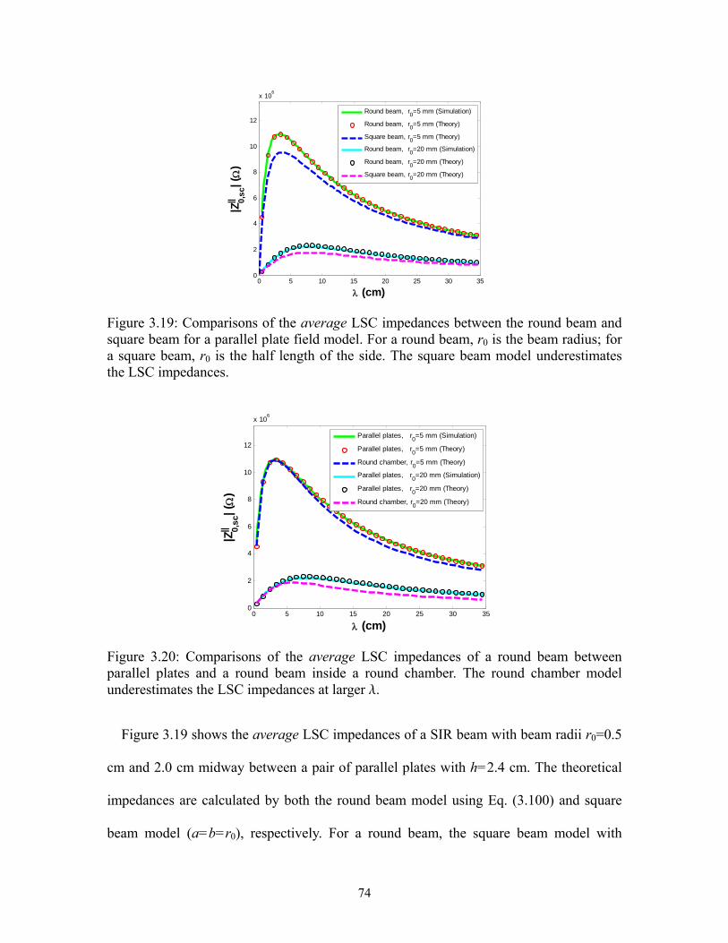
74
Figure 3.19: Comparisons of the average LSC impedances between the round beam and square beam for a parallel plate field model. For a round beam, r0 is the beam radius; for a square beam, r0 is the half length of the side. The square beam model underestimates the LSC impedances.
Figure 3.20: Comparisons of the average LSC impedances of a round beam between parallel plates and a round beam inside a round chamber. The round chamber model underestimates the LSC impedances at larger l.
Figure 3.19 shows the average LSC impedances of a SIR beam with beam radii r0=0.5
cm and 2.0 cm midway between a pair of parallel plates with h=2.4 cm. The theoretical
impedances are calculated by both the round beam model using Eq. (3.100) and square
beam model (a=b=r0), respectively. For a round beam, the square beam model with
0 5 10 15 20 25 30 350
2
4
6
8
10
12
x 106
(cm)
|Z|| 0
,sc| (
)
Round beam, r0=5 mm (Simulation)
Round beam, r0=5 mm (Theory)
Square beam, r0=5 mm (Theory)
Round beam, r0=20 mm (Simulation)
Round beam, r0=20 mm (Theory)
Square beam, r0=20 mm (Theory)
0 5 10 15 20 25 30 350
2
4
6
8
10
12
x 106
(cm)
|Z|| 0
,sc| (
)
Parallel plates, r0=5 mm (Simulation)
Parallel plates, r0=5 mm (Theory)
Round chamber, r0=5 mm (Theory)
Parallel plates, r0=20 mm (Simulation)
Parallel plates, r0=20 mm (Theory)
Round chamber, r0=20 mm (Theory)
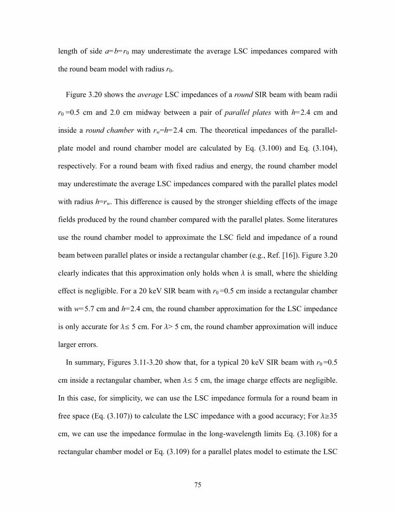
75
length of side a=b=r0 may underestimate the average LSC impedances compared with
the round beam model with radius r0.
Figure 3.20 shows the average LSC impedances of a round SIR beam with beam radii
r0 =0.5 cm and 2.0 cm midway between a pair of parallel plates with h=2.4 cm and
inside a round chamber with rw=h=2.4 cm. The theoretical impedances of the parallel-
plate model and round chamber model are calculated by Eq. (3.100) and Eq. (3.104),
respectively. For a round beam with fixed radius and energy, the round chamber model
may underestimate the average LSC impedances compared with the parallel plates model
with radius h=rw. This difference is caused by the stronger shielding effects of the image
fields produced by the round chamber compared with the parallel plates. Some literatures
use the round chamber model to approximate the LSC field and impedance of a round
beam between parallel plates or inside a rectangular chamber (e.g., Ref. [16]). Figure 3.20
clearly indicates that this approximation only holds when l is small, where the shielding
effect is negligible. For a 20 keV SIR beam with r0 =0.5 cm inside a rectangular chamber
with w=5.7 cm and h=2.4 cm, the round chamber approximation for the LSC impedance
is only accurate for l§ 5 cm. For l> 5 cm, the round chamber approximation will induce
larger errors.
In summary, Figures 3.11-3.20 show that, for a typical 20 keV SIR beam with r0 =0.5
cm inside a rectangular chamber, when l§ 5 cm, the image charge effects are negligible.
In this case, for simplicity, we can use the LSC impedance formula for a round beam in
free space (Eq. (3.107)) to calculate the LSC impedance with a good accuracy; For l¥35
cm, we can use the impedance formulae in the long-wavelength limits Eq. (3.108) for a
rectangular chamber model or Eq. (3.109) for a parallel plates model to estimate the LSC
76
impedance. While for 5 cm<l<35 cm, none of the existing models and formulae can be
used to evaluate the LSC impedance accurately. In this case, we have to use the
approximate theoretical impedance formulae Eqs. (3.102) and (3.103) for a rectangular-
chamber model or Eqs. (3.100) and (3.101) for a parallel-plate model. This is the merit of
the approximate analytical LSC impedance formulae derived in this chapter.
3.5.8 Conclusions for the model of a round beam inside rectangular chamber (between parallel plates)
In this subsection, we mainly derive the approximate average LSC impedance
formulae for a round beam under two boundary conditions: (a) Midway between a pair of
infinitely large, perfectly conducting parallel plates. (b) Inside and coaxial with a
perfectly conducting rectangular chamber. In most accelerators, since w>>r0, h>>r0, the
image charge fields of a round beam can be treated as those of a line charge in calculation
of the LSC fields inside the beam. Consequently, the associated LSC impedances can be
approximated by means of image methods based on the superposition theorem of the
electric fields. The approximate theoretical average LSC impedances of the parallel-plate
model and the rectangular-chamber model are consistent well with the numerical
simulation results in a wide range of the radios of r0/h. In addition, the theoretical LSC
impedances predicted by the two field models also match well with the existing field
models in both the short-wavelength (l§5 cm) and the long-wavelength (lØ35 cm)
limits. In particular, for 5 cm<l<35 cm, the approximate theoretical LSC impedances
formulae have better accuracies than the existing models and formulae. Hence, they are
valid at any perturbation wavelengths and can be used as general expressions of the
average LSC impedances in the future research work on space-charge induced

77
instabilities, even for large ratios of r0/h. At last, the image method together with the line
charge approximation employed in this paper can also be used to derive the LSC
impedances of field models with other cross-sectional geometries.

78
Chapter 4
MICROWAVE INSTABILITY AND LANDAU DAMPING EFFECTS
2
4.1 Introduction
Our previous simulation and experimental results indicated that the instability growth
rates of SIR beam are proportional to the unperturbed beam intensity I0 instead of the
square root of I0 [13]. Pozdeyev [14, 15] and Bi [16] developed their own models and
theories separately to explain the mechanisms of microwave instability in the isochronous
regime, respectively. Pozdeyev pointed out that, in the isochronous regime, the radial
coherent space charge fields of a coasting bunch with centroid wiggling may modify the
slip factor, raise the working point above transition and enhance the microwave instability.
This makes the instability growth rates linearly dependent on the beam intensity [14, 15].
While Bi’s model [16] is not consistent with the scaling law on beam intensity, since the
unperturbed beam density component is neglected in calculation of the coherent radial
space charge force of the perturbed local centroid.
It is also found in the simulations that the spectral evolutions of the line charge
densities are not pure exponential functions of time, instead, they are often characterized
by the betatron oscillations superimposed on the exponential growth curves. These
betatron oscillations are the dipole modes in the longitudinal structure of the beam due to
dipole moment of the centroid offsets [20].
2 Y. Li, L. Wang, F. Lin, Nuclear Instruments and Methods in Physics Research A 763, 674 (2014).
79
In the isochronous regime, the longitudinal motion of particles was usually thought to
be frozen. If and how the Landau damping affects the instability growth rates in the
isochronous regime is still unknown for beam physicists. The theoretical and simulation
studies in this chapter demonstrate that the Landau damping mechanism can also take
effect and suppress the microwave instability for a beam with space charge in the
isochronous regime.
Both Pozdeyev and Bi’s models use the 1D (longitudinal) conventional instability
growth rates formula derived exclusively for a monoenergetic beam and neglects the
emittance effect. As a result, the radial-longitudinal coupling effects in an isochronous
ring are not included completely. This may overestimate the instability growth rates,
especially for the short-wavelength perturbations, because the Landau damping effects
caused by the finite energy spread and the emittance are all neglected. Though Pozdeyev
explained the suppression of the instability growth of short-wavelength perturbations by
the radial-longitudinal coupling effects qualitatively [15], till now, no quantitative
discussions on the Landau damping effects are available for a coasting bunch with space
charge in the isochronous regime.
To predict the microwave instability growth rates more accurately than the existing
conventional 1D formula, this chapter introduces and derives a 2D dispersion relation
with Landau damping effects considering the contributions from both the finite energy
spread and emittance. By doing this, it can explain the suppression of the microwave
instability growth rates of the short-wavelength perturbations and predict the
fastest-growing wavelength.
This chapter is organized as follows. Sect. 4.2 discusses the limitations of the

80
conventional 1D growth rates formula and presents a modified 2D dispersion relation.
Sect. 4.3 discusses the Landau damping effects in the isochronous ring by 2D dispersion
relation. Sect. 4.4 carries out the simulation study of microwave instability in SIR and
provides benchmarking of the 2D dispersion relation with different initial beam
parameters.
4.2 2D dispersion relation
4.2.1 A brief review of the 1D growth rates formula
The conventional 1D growth rates formula for the microwave instability of a
monoenergetic and laminar beam used in Ref. [15] is:
,
2
)()(
20
01
E
kkRZeIik
(4.1)
where 0 is the angular revolution frequency of the on-momentum particles, =–1/2 is
the slip factor, is the momentum compaction factor, is the relativistic energy factor of
the on-momentum particle, e is the electron charge, I0 is the unperturbed beam intensity, k
is the perturbation wavenumber of the longitudinal charge density, R is the average ring
radius, Z(k) is the longitudinal space charge (LSC) impedance, is the relativistic speed
factor, E is the total energy of the on-momentum charged particle. Essentially, the 1D
dispersion relation Eq. (23) of Ref. [16] is the same as the 1D growth rates formula Eq.
(4.1), if we express the LSC field by the LSC impedance.
For the circular SIR beam with radius r0, the transverse dimension of the vacuum
chamber is much greater than the beam diameter. Hence, Ref. [15] neglects the image
charge effects of the chamber in the short-wavelength limits, and chooses Z(k) is equal to
81
the on-axis LSC impedance of the monopole mode [15]:
)],(1[2
)()( 01
02
0
0||,0
krK
kr
rk
RZikZkZ sc (4.2)
where Z0 = 377 Ohm () is the impedance of free space, K1(x) is the modified Bessel
function of the second kind.
For a coasting long bunch with strong space charge effects in the isochronous ring, the
LSC fields may induce the coherent energy deviations and the associated radial offsets of
the local centroids. Consequently, there is centroid wiggling along the bunch. Ref. [15]
assumed that the longitudinal distribution of the radial centroid offsets is a sinusoidal
function of the longitudinal coordinate z with a wavenumber kc. In the first-order
approximation, we can choose k kc and use the same k in the expressions of (k) and
Z(k) in Eq. (4.1) just as treated in Ref. [15] (please check Eqs. (2), (12), (13), and (14) in
Ref. [15]).
Ref. [15] uses the following formalism to derive the space-charge modified coherent
slip factor of a local centroid: due to centroid wiggling, there will be coherent radial
space charge field Ex,sc. It produces positive increments in the dispersion function D
(which is approximated by 2/1 xD ), the momentum compaction factor , and the
coherent slip factor (k). Finally, the space-charge modified coherent slip factor sc(k) can
be determined, i.e., Ex,scDscscsc(k)sc(k). In the end, sc(k) may be
approximated as [14, 15]
)].(1[2
)( 01
02
03
00
0
2
kr
Kkr
Rrm
eIk
H
sc
(4.3)
Note the relativistic factor is introduced in Eq. (4.3) to make the original expressions of

82
sc(k) in Refs. [14, 15] compatible with the high energy beams. Plugging Eqs. (4.2) and
(4.3) into Eq. (4.1) gives the instability growth rates 1/ ∝ [1 − ].
4.2.2 Limitations of 1D growth rates formula
Though the above formalism adopted in Ref. [15] may explain the origin of the
microwave instability of SIR beam and is consistent with the scaling law on beam
intensity, it is not accurate enough and still has some limitations.
First, the LSC impedance in Eq. (4.2) is evaluated from the on-axis LSC field of a 1D
space charge field model. As discussed in Chapter 3, due to the 3D effects on the LSC
fields, Eq. (4.2) should be replaced by the average LSC impedance formula to account
for the LSC field more accurately in the short-wavelength limits:
)].()(21[
2)()( 0
10
120
0||,0
krK
krI
rk
RZikZkZ sc (4.4)
Second, the space-charge modified coherent slip factor is not accurate enough since it
does not include the betatron oscillation effect of the local centroid (please refer to Eq.
(2.30) of Sect. 2.6). In Ref. [42], the transformation of the longitudinal coordinate z with
respect to the bunch center is
,560520510 RxRxRzz (4.5)
where x0 and 0x = dx0/ds are the initial radial betatron motion amplitude and velocity
slope at s=0, respectively, δ=Δp/p is the fractional momentum deviation, R51(s), R52(s),
and R56(s) are the transfer matrix elements and depend on the path length s. Note that in
Ref. [42], was defined differently as the fractional energy deviation =E/E of an
83
ultra-relativistic electron particle with 1, since =p/p(E/E)/2E/E; in addition,
the definition of R51(s), R52(s), and R56(s) in Eq. (4.5) and Ref. [42] are different from the
standard ones (please refer to Appendices A and B for details). For a coasting beam with
space charge in the isochronous ring, in the conventional 1D (longitudinal) beam
dynamics, the space–charge modified parameters of the slip factor sc, the momentum
compaction factor αsc, the transition gamma t,sc, the element R56,sc, and the local
dispersion function Dsc(s) are related to each other by:
,)(111
0
0,56
22,
2 C
CR sc
sctscsc
(4.6)
,)(
)(
)(
)(11)(1
02
0
0,56
2,
s
sDds
s
sD
CC
CRsc
L
scsc
sctsc
(4.7)
where (s) is the local radius of curvature of trajectory, <ÿÿÿ> denotes the average value
over the ring circumference C0. From Eqs. (4.6), (4.7) and the formalism used in Ref.
[15], we can see that only the contribution of the momentum compaction factor sc or the
element R56,sc is considered in the modification of sc(k). While Eq. (4.5) shows z =z-z0
is determined by R51, R52, and R56, the ring is isochronous if z=0 after one revolution.
The space-charge modified coherent slip factor of a local centroid should be dependent
on both R56 and R51, R52. In Ref. [42], where the method of characteristics is employed,
the parameters x0, 0x , and z0, at s=0 are regarded as constants of motion, they are related
to the current coordinates of the particle x, x and z at position s by a canonical
transformation
,
sin)](
ˆˆ
'[ˆˆcos)(ˆ
ˆ),,,( 0
00 DxDxDxsxxx

84
,
cos)](ˆˆ
[ˆ
ˆsin
ˆˆ),,,(
00
0 DxDxDx
sxxx
(4.8)
,( 520510560 ),,, RxRxRzsxxz
where , ,0 and are the Courant-Snyder parameters, y is the phase advance. Their
derivatives with respect to δ are
,
sin)
ˆˆ
(ˆˆcosˆ
ˆ0
00 DDDx
,
cos)
ˆˆ
(ˆ
ˆsin
ˆˆ 00
0 DDDx
(4.9)
,520
510
560 R
xR
xR
z
which usually are non-zero parameters. Accordingly, the exact expression of the slip
factor at s can be calculated as (s, k)=-(dDz/d)/C0= -[R51(s, s+C0)∑x0/∑+R52(s, s+C0)
∑ /∑ +R56(s, s+C0)]/C0, and it also depends on R51(s, s+C0), R52(s, s+C0) if ∑x0/∑0
and ∑ /∑0. Here R51(s, s+C0), R52(s, s+C0) and R56(s, s+C0) are the transfer matrix
elements between s and s+C0. The space–charge modified slip factor expressed in Eq.
(4.6) is only a special case at s=0, ∑ x0/∑ =0, and ∑ /∑=0. The contributions of R51,sc
and R52,sc to the coherent slip factor are related to the betatron motion of the centroid and
should not be neglected in the isochronous regime.
Third, Ref. [15] only takes into account the coherent motion of the local beam centroid
neglecting the incoherent motions of individual particles in the beam slices. In fact, a
local beam slice usually has a finite energy spread and emittance. Eq. (4.5) and the above
analysis indicate that, the betatron motions of particles in a beam slice with different d, x0,

85
and may have different longitudinal path length differences Dz which are not the
same as that of the local centroid. This may cause smearing of the beam intensity
perturbations and is the very reason of Landau damping.
4.2.3 Space-charge modified tunes and transition gammas in the isochronous regime
The radial space charge fields may modify the radial tunes and transition gammas in
the isochronous regime [14-16]. Due to the large ratios between the full chamber width
(~11.4 cm), full chamber gap (~4.8 cm) and the beam diameter (~1 cm), the image
charge effects caused by the vacuum chamber are small for perturbation wavelength l§ 5
cm as shown in Chapter 3. Then Pozdeyev’s model [14, 15] of a uniform circular beam
with centroid wiggling in free space can be used to calculate the radial space charge fields
and modified tunes. Assuming the total radial offset of a particle is x=xc +xβ, where xc is
the beam centroid offset xc=accos(kz), k is the wavenumber of radial offset perturbations
of local beam centroids with respect to the design orbit along z, xβ is the radial offset of a
single particle due to the betatron oscillation. The equations of coherent and incoherent
radial motions can be expressed as:
,22
,2
2
2cm
eE
Rx
R
vx
H
cohxcohc
xc
(4.10)
,22
,2
2
2cm
eE
Rx
R
vx
H
incxincx
(4.11)
where nx is the bare radial betatron tune, coh and inc are the coherent and incoherent
fractional momentum deviations, Ex,coh and Ex,inc are the coherent and incoherent radial
space charge fields [15, 16], respectively, and can be expressed as

86
,/2
0,2
exmE cHcohcohx
./20,
2exmE
Hincincx
(4.12)
Here
)],(1[2
01
02
03
00
0
2
kr
Kkr
Rrm
eI
H
coh
,Rrm
eI
H
inc 20
300
0
22
(4.13)
are two unitless parameters. For a typical SIR beam with 0 < coh << 1 and 0 < inc << 1,
the coherent and incoherent radial tunes can be easily obtained from Eqs. (4.10)-(4.13) as
),2
1(2,x
cohxcohx v
).2
1(2,x
incxincx v
(4.14)
Here the coherent radial tune x,coh and incoherent radial tune x,inc stand for the number
of betatron oscillations per revolution of a local centroid and a single particle,
respectively. According to Ref. [16], the space-charge modified coherent and incoherent
transition gammas in an isochronous accelerator are
,1
/
/2, cohcoht n
RR
pp
,1
/
/2, incinct n
RR
pp
(4.15)
where n= -(r/B)(∑B/∑r) is the magnetic field index. For the SIR with n < 0, |n|<<1, if the
space charge effects are negligible (i.e., coh=inc =0, nt 120, ), the bare slip factor is 0
= 220, /1/1 t
2/11 n 2 10-4. Then
,
11022
,coh
coht
.11
022,
incinct
(4.16)
4.2.4 2D dispersion relation
For a hot beam with large energy spread and emittance in an isochronous ring, the
Landau damping effects are important due to the strong radial-longitudinal coupling.

87
Hence, a multi-dimensional dispersion relation including both the longitudinal and radial
dynamics is needed. Usually the vertical motions of particles can be regarded as
decoupled from their radial and longitudinal motions. In this section, first, we would like
to summarize and comment the main procedures and definitions used in Ref. [42], where
a 2D (longitudinal and radial) dispersion relation was derived for the coherent
synchrotron radiation (CSR) instability of an ultra-relativistic electron beam in a
conventional storage ring. Based on this model, we can derive a 2D dispersion relation
for the microwave instability of the non-relativistic beam in an isochronous ring.
4.2.4.1 Review of the 2D dispersion relation for CSR instability of ultra-relativistic electron beams in non-isochronous regime
First, Ref. [42] defined a 2D Gaussian beam model with an initial equilibrium beam
distribution function
),ˆ(]ˆ2
)'ˆ(exp[
2 0
00,
200
20
0,0 zug
xxnf
xx
b
(4.17)
where ),2
exp(2
1)( 2
2
g (4.18)
nb is the linear number density of the beam, εx,0 is the initial radial emittance, x0 is the
initial radial offset, 0x =dx0/ds is the initial radial velocity slope, 0 is the betatron
function at s=0, d is the uncorrelated fractional momentum deviation, u is the chirp
parameter which accounts for the correlation between the longitudinal position z of the
particle in the bunch and its fractional momentum deviation d, δ is the uncorrelated
fractional RMS momentum spread (Note in Ref. [42], δ was defined differently as the
uncorrelated fractional RMS energy spread for an ultra-relativistic electron beam with
88
1). Then the perturbed distribution function f1 is assumed to have a sinusoidal
dependence on z0 as
,),,,(),,,,( 000000001
ikzk esxxfszxxf (4.19)
where 00 ˆzu is the total fractional momentum deviation including both the
uncorrelated and correlated fractional momentum deviation. Plugging the distribution
function of f=f0+f1 into the linearized Vlasov equation, after lengthy derivations, a
Volterra integral equation is derived as
, s
kkk sdsgssKsgsg0
)0( )(),()()( (4.20)
where
,)]()()()[(exp),,,()( 520510560000000 sRxsRxsRsikCsxxfdxddxsg kk (4.21)
,)]()()()[(exp)0,,,()( 520510560000000)0( sRxsRxsRsikCxxfdxddxsg kk (4.22)
,)(ˆ1
1)(
56 sRusC
(4.23)
is the bunch length compression factor, K(s£, s) is the kernel of integration. The perturbed
harmonic line density with wave number k at (z, s) is
.)()(),( )(C1000,1
zsikkk esgsCfdxddxszn (4.24)
We can see that |C(s)gk(s)| is just the amplitude of the perturbed line density at s. For
storage rings, the linear chirp factor 0ˆ u , the compression factor C(s) =1. By smooth
approximations of Rxxx /20, , xR /ˆ , Rsx / , 2/ xRD , 0ˆ , 0D , the integral
kernel in Eq. (4.20) is simplified as
)(),( 1 KssK
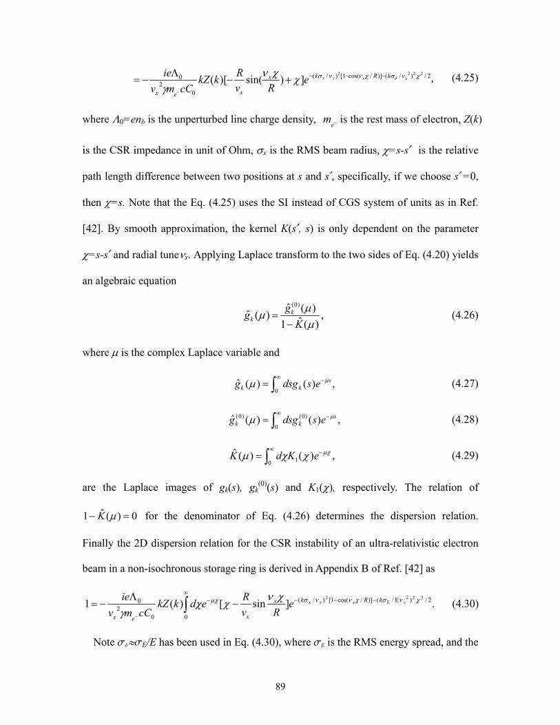
89
,2/)/()]/cos(1[)/(
02
02222
])sin()[(
xxxx kRkx
xex
eRv
RkkZ
cCmv
ie
(4.25)
where 0=enb is the unperturbed line charge density, em is the rest mass of electron, Z(k)
is the CSR impedance in unit of Ohm, x is the RMS beam radius, =s-s£ is the relative
path length difference between two positions at s and s£, specifically, if we choose s£ =0,
then =s. Note that the Eq. (4.25) uses the SI instead of CGS system of units as in Ref.
[42]. By smooth approximation, the kernel K(s£, s) is only dependent on the parameter
=s-s£ and radial tunex. Applying Laplace transform to the two sides of Eq. (4.20) yields
an algebraic equation
,)(ˆ1
)(ˆ)(ˆ
)0(
K
gg k
k (4.26)
where is the complex Laplace variable and
,)()(ˆ0 s
kk esdsgg (4.27)
,)()(ˆ0
)0()0( s
kk esdsgg (4.28)
,)()(ˆ0 1 eKdK (4.29)
are the Laplace images of gk(s), gk(0)(s) and K1(), respectively. The relation of
0)(ˆ1 K for the denominator of Eq. (4.26) determines the dispersion relation.
Finally the 2D dispersion relation for the CSR instability of an ultra-relativistic electron
beam in a non-isochronous storage ring is derived in Appendix B of Ref. [42] as
.]sin[)(1 2/)E/()]/cos(1[)/(
002
0222
E2
xxxx kRkx
xex
eRv
RedkkZ
cCmv
ie
(4.30)
Note sdºsE/E has been used in Eq. (4.30), where sE is the RMS energy spread, and the

90
SI system of units is used in Eq. (4.30). Eq. (4.30) is an integral equation which
determines the relations between the wavenumber k and the complex Laplace variable .
For a fixed k, the values of can be solved numerically.
Ref. [42] did not explicitly interpret the CSR instability growth rates from the solutions
to Eq. (4.30). Theoretically speaking, gk(s) can be calculated by inverse Laplace
transform (Fourier-Mellin transform)
,)(
i
i
skk e
K
gd
isg
)(ˆ1
ˆ
2
1)(
)0(
(4.31)
where is a positive real number. The integration is along the Bromwich contour, which
is a line parallel to the imaginary -axis and to the right of all the singularities satisfying
0)(ˆ1 K in the complex -plane. In practice, the integral in Eq. (4.31) poses a great
difficulty in mathematics due to complexity of the integrand. A popular method dealing
with this difficulty is widely used in the Plasma Physics [43-46] by applying Cauchy’s
residue theory to an equivalent Bromwich contour. First, the Bromwich contour is
deformed by analytic continuation, and then the solutions of gk(s) can be evaluated by the
residues of the poles using Cauchy’s residue theorem as
jjk
j
sskj
uj
js
kk gRsdeegegRsdsg j
j
,]),(ˆ[])(ˆ)[(lim],)(ˆ[)(
(4.32)
where ]),(ˆ[ jkgRsd stands for the residue of )(ˆ kg at the pole j. Using the relation s
= ct, where t is the time, the temporal evolution of gk(s) becomes
j
jkct
k gRsdetg j ].),(ˆ[)( (4.33)
For a storage ring, C(s)=1, Eq. (4.24) gives the amplitude of perturbed harmonic line
density with wavenumber k as
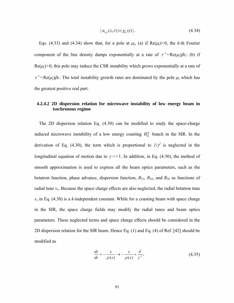
91
.|)(||),(| ,1 tgtzn kk (4.34)
Eqs. (4.33) and (4.34) show that, for a pole at j, (a) if Re(j)<0, the k-th Fourier
component of the line density damps exponentially at a rate of 1- =Re(j)c; (b) if
Re(j)>0, this pole may induce the CSR instability which grows exponentially at a rate of
1- =Re(j)c. The total instability growth rates are dominated by the pole j which has
the greatest positive real part.
4.2.4.2 2D dispersion relation for microwave instability of low energy beam in isochronous regime
The 2D dispersion relation Eq. (4.30) can be modified to study the space-charge
induced microwave instability of a low energy coasting bunch in the SIR. In the
derivation of Eq. (4.30), the term which is proportional to 1/2 is neglected in the
longitudinal equation of motion due to >>1. In addition, in Eq. (4.30), the method of
smooth approximation is used to express all the beam optics parameters, such as the
betatron function, phase advance, dispersion function, R51, R52, and R56 as functions of
radial tune νx. Because the space charge effects are also neglected, the radial betatron tune
νx in Eq. (4.30) is a k-independent constant. While for a coasting beam with space charge
in the SIR, the space charge fields may modify the radial tunes and beam optics
parameters. These neglected terms and space charge effects should be considered in the
2D dispersion relation for the SIR beam. Hence Eq. (1) and Eq. (4) of Ref. [42] should be
modified as
,)()( 2
s
x
s
x
ds
dz
(4.35)
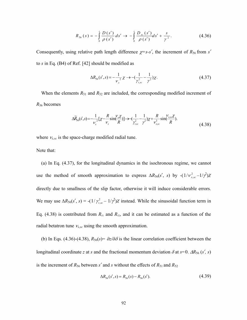
92
.)(
)(
)(
)()(
200
56 s
sds
sDsd
s
sDsR
ssc
s
(4.36)
Consequently, using relative path length difference =s-s£, the increment of R56 from s£
to s in Eq. (B4) of Ref. [42] should be modified as
.)11
(1
),( 22,
256
sctx
ssR
(4.37)
When the elements R51 and R52 are included, the corresponding modified increment of
R56 becomes
).sin()11
()]sin([1
),(~ ,
3,
22,
256 R
R
R
RssR scx
scxsct
x
xx
(4.38)
where x,sc is the space-charge modified radial tune.
Note that:
(a) In Eq. (4.37), for the longitudinal dynamics in the isochronous regime, we cannot
use the method of smooth approximation to express R56(s£, s) by -( 2
,/1 scx –1/2)
directly due to smallness of the slip factor, otherwise it will induce considerable errors.
We may use R56(s£, s) = -( 2
,/1 sct – 1/2) instead. While the sinusoidal function term in
Eq. (4.38) is contributed from R51 and R52, and it can be estimated as a function of the
radial betatron tune x,sc using the smooth approximation.
(b) In Eqs. (4.36)-(4.38), R56(s)= ∑z/∑ is the linear correlation coefficient between the
longitudinal coordinate z at s and the fractional momentum deviation at s=0. R56 (s£, s)
is the increment of R56 between s£ and s without the effects of R51 and R52
).()(),( 565656 sRsRssR (4.39)
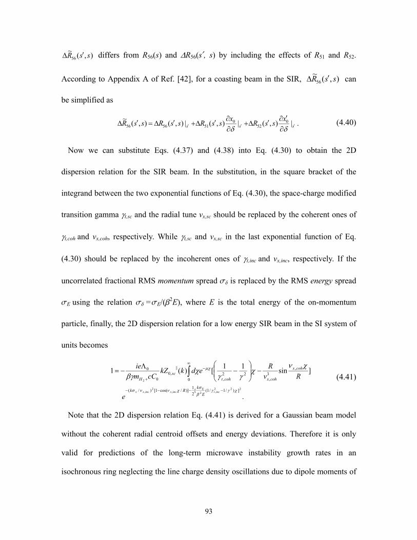
93
),(~
56 ssR differs from R56(s) and R56(s£, s) by including the effects of R51 and R52.
According to Appendix A of Ref. [42], for a coasting beam in the SIR, ),(~
56 ssR can
be simplified as
.|),(|),(|),(),(~ 0
520
515656 sss
xssR
xssRssRssR
(4.40)
Now we can substitute Eqs. (4.37) and (4.38) into Eq. (4.30) to obtain the 2D
dispersion relation for the SIR beam. In the substitution, in the square bracket of the
integrand between the two exponential functions of Eq. (4.30), the space-charge modified
transition gamma t,sc and the radial tune νx,sc should be replaced by the coherent ones of
t,coh and νx,coh, respectively. While t,sc and νx,sc in the last exponential function of Eq.
(4.30) should be replaced by the incoherent ones of t,inc and νx,inc, respectively. If the
uncorrelated fractional RMS momentum spread sd is replaced by the RMS energy spread
sE using the relation sd =sE/(b2E), where E is the total energy of the on-momentum
particle, finally, the 2D dispersion relation for a low energy SIR beam in the SI system of
units becomes
.
]sin11
[)(1
222,2
E,
2,
2
])/1/1([2
1)]/cos(1[)/(
,
03,
22,
||,0
0
0
inctincxincxxE
kRk
cohx
cohxcohtsc
H
e
Rv
RedkkZ
cCm
ie
(4.41)
Note that the 2D dispersion relation Eq. (4.41) is derived for a Gaussian beam model
without the coherent radial centroid offsets and energy deviations. Therefore it is only
valid for predictions of the long-term microwave instability growth rates in an
isochronous ring neglecting the line charge density oscillations due to dipole moments of

94
the centroid offsets. Here the term ‘long-term’ stands for multi-periods of betatron
oscillations in the time scale. When the dispersion relation Eq. (4.41) is to be solved
numerically, a large but finite real number can be set as the upper limit of c instead of
infinity to calculate the integral.
4.3 Landau damping effects in isochronous ring
4.3.1 Space-charge modified coherent slip factors
For the SIR beam with typical beam intensities, usually |0| << coh, when the space
charge effects are considered. Then in the first-order approximation, according to Eq.
(4.16), the space-charge modified coherent slip factor without the effects of R51 and R52
(e.g., neglect the betatron motion effects) may be estimated as
,11
02,
256R cohcohcoht
coh
(4.42)
which is essentially the same as Eq. (12) in Ref. [15].
For a ring lattice with average radius R and space-charge modified radial tune nx,sc, by
smooth approximation of xR /ˆ , Rsx / , 2/ xRD , 0ˆ , 0D , the increments of
R51 and R52 between s£ and s can be calculated from Eq. (B2) and Eq. (4) of Ref. [42] as
)],sin()[sin(1
-),( ,,
,51 s
R
vs
RssR scxscx
scx
(4.43)
)].cos()(cos[1
),( ,,2,
52 sR
vs
RssR scxscx
scx
(4.44)
According to Eq. (4.9) (i.e., Eq. (20) of Ref. [42]),
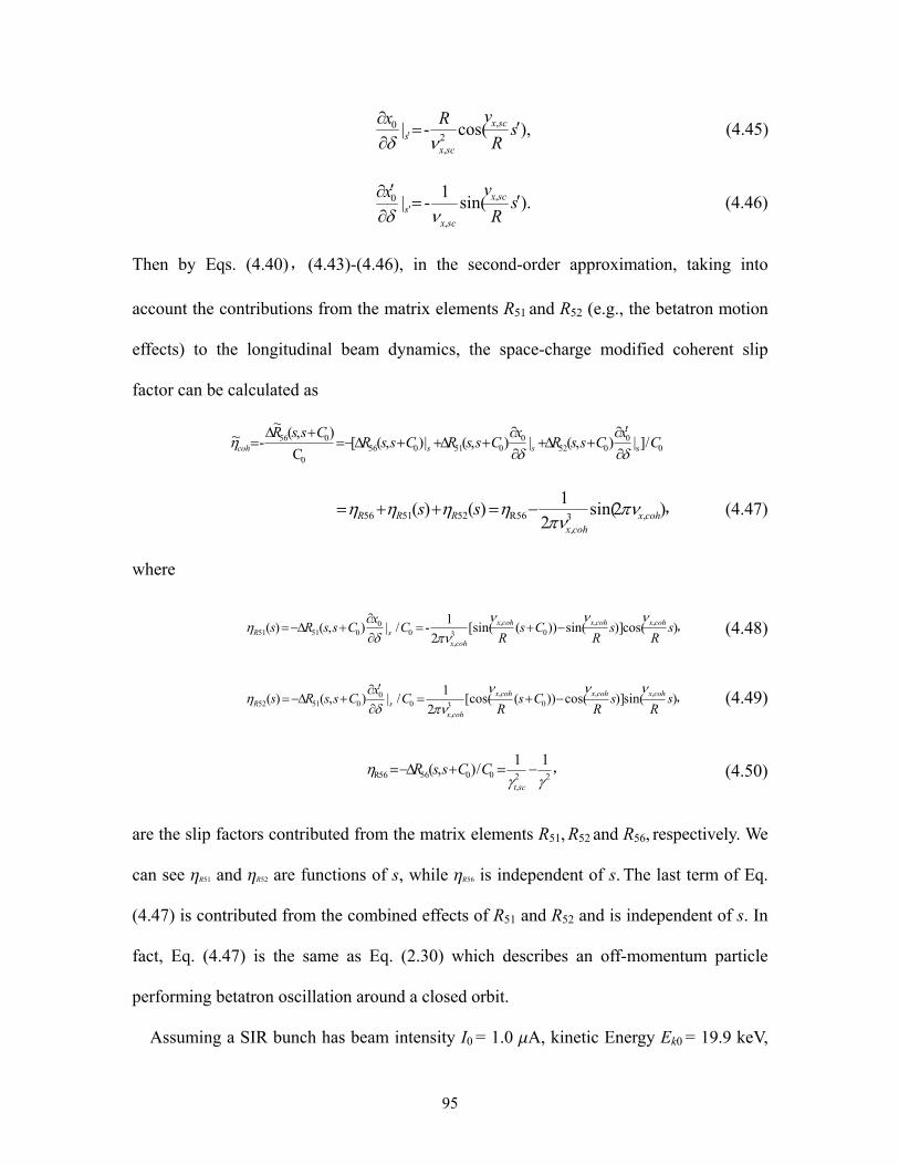
95
),cos(-| ,
2,
0 sR
vRx scx
scxs
(4.45)
).sin(1
-| ,
,'
0 sR
vx scx
scxs
(4.46)
Then by Eqs. (4.40),(4.43)-(4.46), in the second-order approximation, taking into
account the contributions from the matrix elements R51 and R52 (e.g., the betatron motion
effects) to the longitudinal beam dynamics, the space-charge modified coherent slip
factor can be calculated as
0s0
0520
0510560
056 /]|),(|),(|),([C
),(~
-~ Cx
CssRx
CssRCssRCssR
sscoh
,)2sin(2
1)()( ,3
,R56525156 cohx
cohxRRR ss
(4.47)
where
,)cos()]sin())([sin(2
1-/|),()( ,,
0,
3,
00
05151 sR
sR
CsR
Cx
CssRs cohxcohxcohx
cohxsR
(4.48)
,)sin()]cos())([cos(2
1/|),()( ,,
0,
3,
00
05152 sR
sR
CsR
Cx
CssRs cohxcohxcohx
cohxsR
(4.49)
,22
,
005656R
11/),(
sct
CCssR
(4.50)
are the slip factors contributed from the matrix elements R51, R52 and R56, respectively. We
can see hR51 and hR52 are functions of s, while hR56 is independent of s. The last term of Eq.
(4.47) is contributed from the combined effects of R51 and R52 and is independent of s. In
fact, Eq. (4.47) is the same as Eq. (2.30) which describes an off-momentum particle
performing betatron oscillation around a closed orbit.
Assuming a SIR bunch has beam intensity I0 = 1.0 mA, kinetic Energy Ek0 = 19.9 keV,
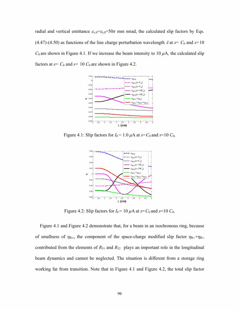
96
radial and vertical emittance x,0=y,0=50p mm mrad, the calculated slip factors by Eqs.
(4.47)-(4.50) as functions of the line charge perturbation wavelength l at s= C0 and s=10
C0 are shown in Figure 4.1. If we increase the beam intensity to 10 mA, the calculated slip
factors at s= C0 and s= 10 C0 are shown in Figure 4.2.
Figure 4.1: Slip factors for I0 = 1.0 mA at s=C0 and s=10 C0.
Figure 4.2: Slip factors for I0 = 10 mA at s=C0 and s=10 C0.
Figure 4.1 and Figure 4.2 demonstrate that, for a beam in an isochronous ring, because
of smallness of hR56, the component of the space-charge modified slip factor hR51+hR52
contributed from the elements of R51 and R52 plays an important role in the longitudinal
beam dynamics and cannot be neglected. The situation is different from a storage ring
working far from transition. Note that in Figure 4.1 and Figure 4.2, the total slip factor
0 0.5 1 1.5 2 2.5 3 3.5 4 4.5 5-0.09
-0.08
-0.07
-0.06
-0.05
-0.04
-0.03
-0.02
-0.01
0
0.01
(cm)
R56
R51(s=C0)
R52(s=C0)
R51(s=10C0)
R52(s=10C0)
R51+R52
R51+R52+R56
0 0.5 1 1.5 2 2.5 3 3.5 4 4.5 5-0.08
-0.06
-0.04
-0.02
0
0.02
0.04
0.06
0.08
(cm)
R56
R51(s=C0)
R52(s=C0)
R51(s=10C0)
R52(s=10C0)
R51+R52
R51+R52+R56
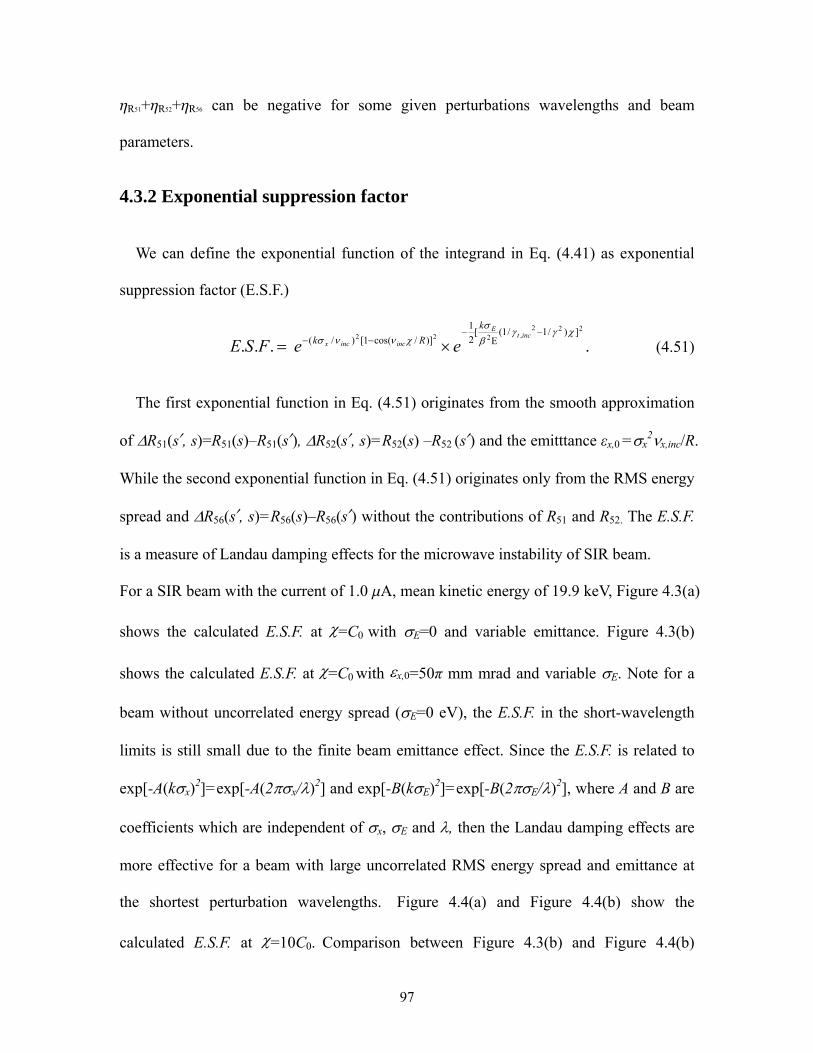
97
hR51+hR52+hR56 can be negative for some given perturbations wavelengths and beam
parameters.
4.3.2 Exponential suppression factor
We can define the exponential function of the integrand in Eq. (4.41) as exponential
suppression factor (E.S.F.)
. ...222
,222 ])/1/1(E
[2
1
)]/cos(1[)/(
inct
E
incincx
k
Rk eeFSE (4.51)
The first exponential function in Eq. (4.51) originates from the smooth approximation
of R51(s£, s)=R51(s)–R51(s
£), R52(s£, s)=R52(s) –R52 (s
£) and the emitttance εx,0 =x2x,inc/R.
While the second exponential function in Eq. (4.51) originates only from the RMS energy
spread and R56(s£, s)=R56(s)–R56(s
£) without the contributions of R51 and R52. The E.S.F.
is a measure of Landau damping effects for the microwave instability of SIR beam.
For a SIR beam with the current of 1.0 mA, mean kinetic energy of 19.9 keV, Figure 4.3(a)
shows the calculated E.S.F. at =C0 with E=0 and variable emittance. Figure 4.3(b)
shows the calculated E.S.F. at =C0 with x,0=50π mm mrad and variable E. Note for a
beam without uncorrelated energy spread (E=0 eV), the E.S.F. in the short-wavelength
limits is still small due to the finite beam emittance effect. Since the E.S.F. is related to
exp[-A(kx)2]=exp[-A(2x/)2] and exp[-B(kE)2]=exp[-B(2E/)2], where A and B are
coefficients which are independent of x, E and , then the Landau damping effects are
more effective for a beam with large uncorrelated RMS energy spread and emittance at
the shortest perturbation wavelengths. Figure 4.4(a) and Figure 4.4(b) show the
calculated E.S.F. at =10C0. Comparison between Figure 4.3(b) and Figure 4.4(b)
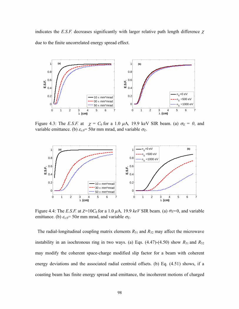
98
indicates the E.S.F. decreases significantly with larger relative path length difference
due to the finite uncorrelated energy spread effect.
Figure 4.3: The E.S.F. at = C0 for a 1.0 mA, 19.9 keV SIR beam. (a) E = 0, and variable emittance. (b) x,0= 50π mm mrad, and variable E.
Figure 4.4: The E.S.F. at =10C0 for a 1.0 mA, 19.9 keV SIR beam. (a) E=0, and variable emittance. (b) x,0= 50π mm mrad, and variable E.
The radial-longitudinal coupling matrix elements R51 and R52 may affect the microwave
instability in an isochronous ring in two ways. (a) Eqs. (4.47)-(4.50) show R51 and R52
may modify the coherent space-charge modified slip factor for a beam with coherent
energy deviations and the associated radial centroid offsets. (b) Eq. (4.51) shows, if a
coasting beam has finite energy spread and emittance, the incoherent motions of charged
0 1 2 3 4 5 6 7
0
0.2
0.4
0.6
0.8
1
(cm)
E.S
.F.
10 mm*mrad30 mm*mrad50 mm*mrad
(a)
0 1 2 3 4 5 6 7
0
0.2
0.4
0.6
0.8
1
(cm)
E.S
.F.
E=0 eV
E =500 eV
E =1000 eV
(b)
0 1 2 3 4 5 6 7
0
0.2
0.4
0.6
0.8
1
(cm)
E.S
.F.
10 mm*mrad30 mm*mrad50 mm*mrad
(a)
0 1 2 3 4 5 6 7
0
0.2
0.4
0.6
0.8
1
(cm)
E.S
.F.
E=0 eV
E =500 eV
E =1000 eV
(b)

99
particles under the effects of matrix elements R51, R52 and R56 may produce a finite spread
in the longitudinal motion spectrum around the revolution frequency. The revolution
frequency spread can help to smear out the longitudinal charge density modulations and
suppress the microwave instability growth rates, especially for the short-wavelength
perturbations. This is the origin of the Landau damping effects in the isochronous regime.
Since the matrix elements R51, R52 and R56 may affect the beam instability in such a
complicated way, it is difficult to predict how the instability growth rates will change if
only one of these elements is increased or decreased.
4.3.3 Relations between the 1D growth rates formula and 2D dispersion relation
In the 2D dispersion relation Eq. (4.41), if we neglect the E.S.F. (incoherent motion
effects of single particle) and the sinusoidal term in the square bracket of the integrand
which originates from the coupling matrix elements R51(s) and R52(s) (coherent betatron
motion effects of the local centroids), the 2D dispersion relation is reduced to
.11
)(10
22,
||,0
0
0
2
cohtsc
H
edkkZcCm
ie (4.52)
With Eq. (4.42) and the equality of
,1
20
sdse s (4.53)
the simplified 2D dispersion relation Eq. (4.52) can be reduced further as
.
2)(
2
||,00
01
E
kRZeIick sccoh
(4.54)
Eq. (4.54) is just the Eq. (4.1) for a 1D monoenergetic beam.
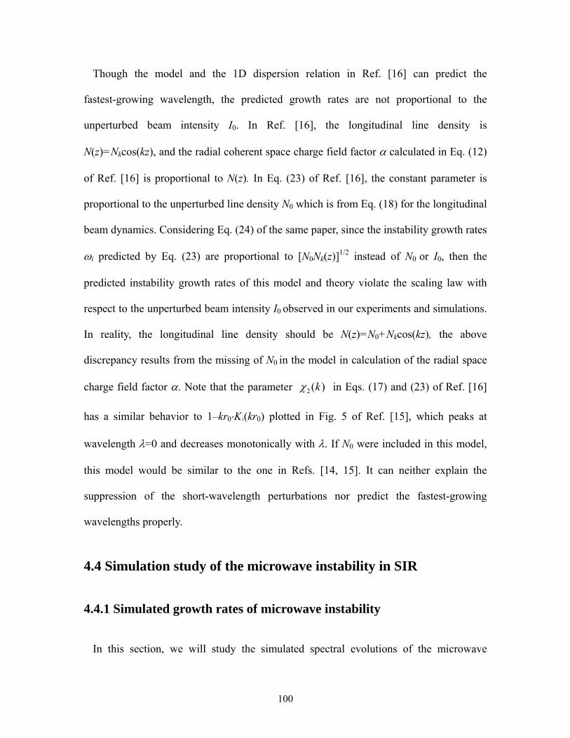
100
Though the model and the 1D dispersion relation in Ref. [16] can predict the
fastest-growing wavelength, the predicted growth rates are not proportional to the
unperturbed beam intensity I0. In Ref. [16], the longitudinal line density is
N(z)=Nkcos(kz), and the radial coherent space charge field factor calculated in Eq. (12)
of Ref. [16] is proportional to N(z). In Eq. (23) of Ref. [16], the constant parameter is
proportional to the unperturbed line density N0 which is from Eq. (18) for the longitudinal
beam dynamics. Considering Eq. (24) of the same paper, since the instability growth rates
i predicted by Eq. (23) are proportional to [N0Nk(z)]1/2 instead of N0 or I0, then the
predicted instability growth rates of this model and theory violate the scaling law with
respect to the unperturbed beam intensity I0 observed in our experiments and simulations.
In reality, the longitudinal line density should be N(z)=N0+Nkcos(kz), the above
discrepancy results from the missing of N0 in the model in calculation of the radial space
charge field factor . Note that the parameter )(2 k in Eqs. (17) and (23) of Ref. [16]
has a similar behavior to 1–kr0K1(kr0) plotted in Fig. 5 of Ref. [15], which peaks at
wavelength =0 and decreases monotonically with . If N0 were included in this model,
this model would be similar to the one in Refs. [14, 15]. It can neither explain the
suppression of the short-wavelength perturbations nor predict the fastest-growing
wavelengths properly.
4.4 Simulation study of the microwave instability in SIR
4.4.1 Simulated growth rates of microwave instability
In this section, we will study the simulated spectral evolutions of the microwave
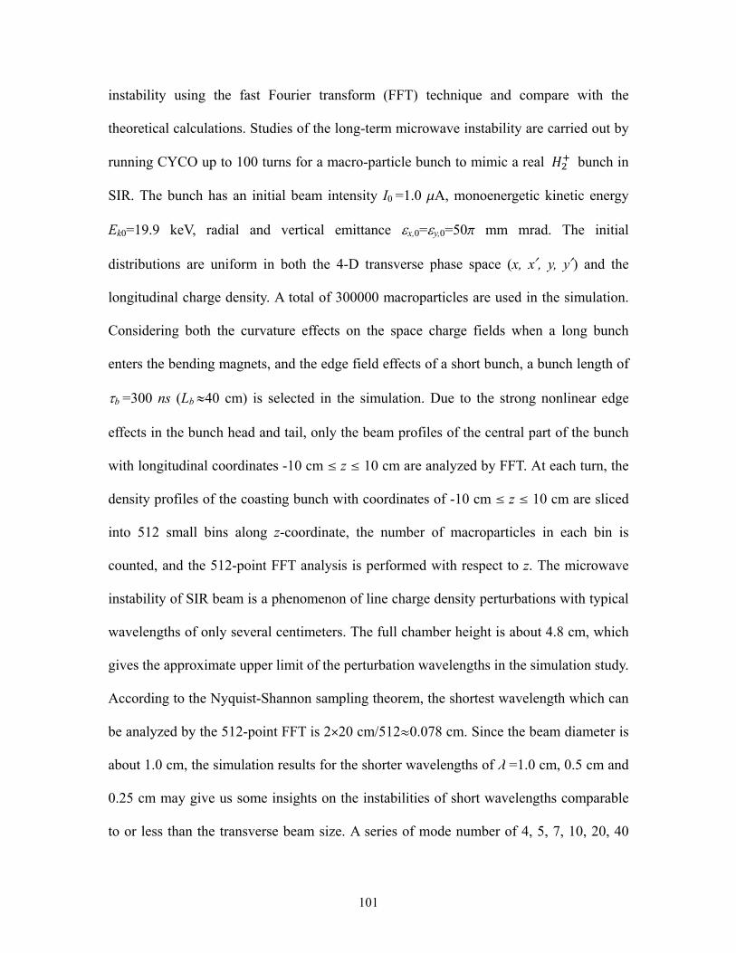
101
instability using the fast Fourier transform (FFT) technique and compare with the
theoretical calculations. Studies of the long-term microwave instability are carried out by
running CYCO up to 100 turns for a macro-particle bunch to mimic a real bunch in
SIR. The bunch has an initial beam intensity I0 =1.0 mA, monoenergetic kinetic energy
Ek0=19.9 keV, radial and vertical emittance x,0=y,0=50p mm mrad. The initial
distributions are uniform in both the 4-D transverse phase space (x, x£, y, y£) and the
longitudinal charge density. A total of 300000 macroparticles are used in the simulation.
Considering both the curvature effects on the space charge fields when a long bunch
enters the bending magnets, and the edge field effects of a short bunch, a bunch length of
b =300 ns (Lb 40 cm) is selected in the simulation. Due to the strong nonlinear edge
effects in the bunch head and tail, only the beam profiles of the central part of the bunch
with longitudinal coordinates -10 cm § z § 10 cm are analyzed by FFT. At each turn, the
density profiles of the coasting bunch with coordinates of -10 cm § z § 10 cm are sliced
into 512 small bins along z-coordinate, the number of macroparticles in each bin is
counted, and the 512-point FFT analysis is performed with respect to z. The microwave
instability of SIR beam is a phenomenon of line charge density perturbations with typical
wavelengths of only several centimeters. The full chamber height is about 4.8 cm, which
gives the approximate upper limit of the perturbation wavelengths in the simulation study.
According to the Nyquist-Shannon sampling theorem, the shortest wavelength which can
be analyzed by the 512-point FFT is 2ä20 cm/512º0.078 cm. Since the beam diameter is
about 1.0 cm, the simulation results for the shorter wavelengths of l =1.0 cm, 0.5 cm and
0.25 cm may give us some insights on the instabilities of short wavelengths comparable
to or less than the transverse beam size. A series of mode number of 4, 5, 7, 10, 20, 40
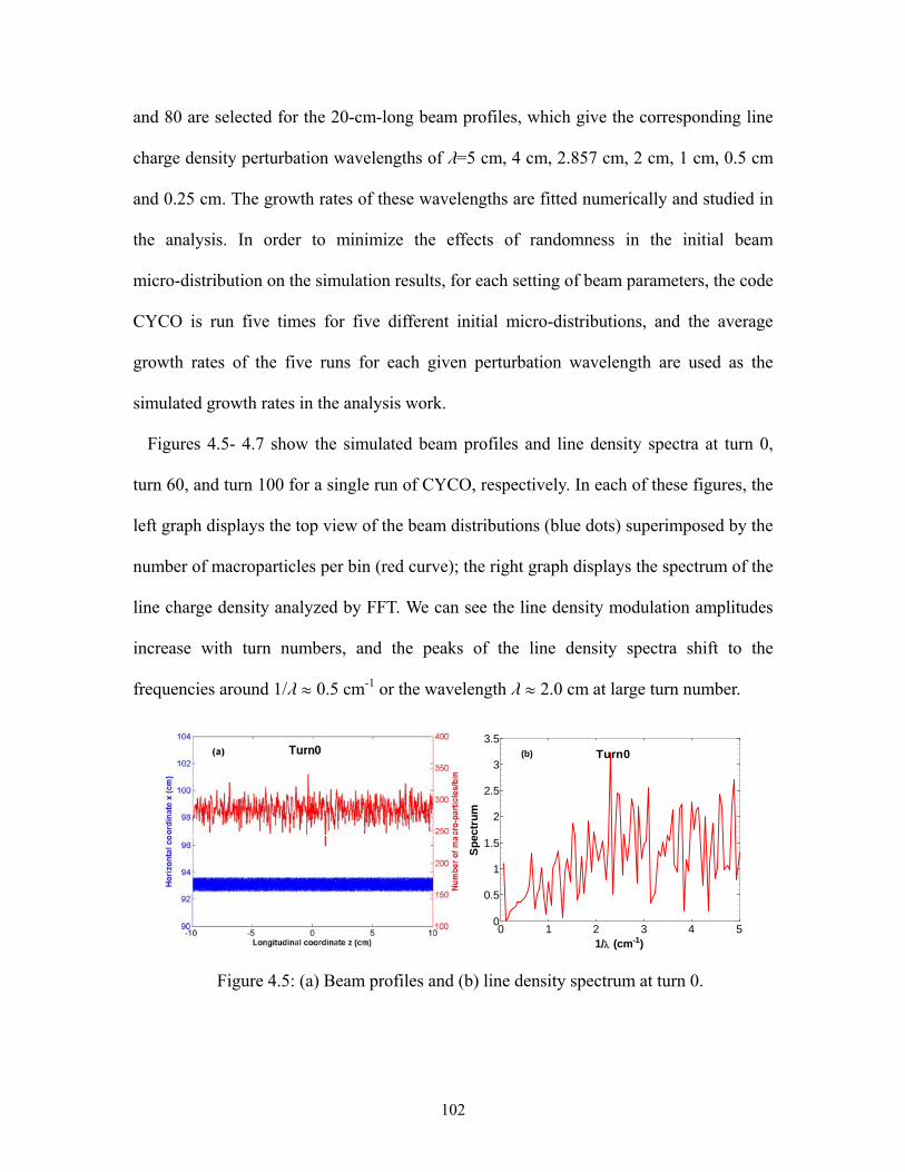
102
and 80 are selected for the 20-cm-long beam profiles, which give the corresponding line
charge density perturbation wavelengths of l=5 cm, 4 cm, 2.857 cm, 2 cm, 1 cm, 0.5 cm
and 0.25 cm. The growth rates of these wavelengths are fitted numerically and studied in
the analysis. In order to minimize the effects of randomness in the initial beam
micro-distribution on the simulation results, for each setting of beam parameters, the code
CYCO is run five times for five different initial micro-distributions, and the average
growth rates of the five runs for each given perturbation wavelength are used as the
simulated growth rates in the analysis work.
Figures 4.5- 4.7 show the simulated beam profiles and line density spectra at turn 0,
turn 60, and turn 100 for a single run of CYCO, respectively. In each of these figures, the
left graph displays the top view of the beam distributions (blue dots) superimposed by the
number of macroparticles per bin (red curve); the right graph displays the spectrum of the
line charge density analyzed by FFT. We can see the line density modulation amplitudes
increase with turn numbers, and the peaks of the line density spectra shift to the
frequencies around 1/l º 0.5 cm-1 or the wavelength l º 2.0 cm at large turn number.
Figure 4.5: (a) Beam profiles and (b) line density spectrum at turn 0.
0 1 2 3 4 50
0.5
1
1.5
2
2.5
3
3.5
1/ (cm-1)
Sp
ectr
um
Turn0(b)
103
Figure 4.6: (a) Beam profiles and (b) line density spectrum at turn 60.
Figure 4.7: (a) Beam profiles and (b) line density spectrum at turn 100.
Figure 4.8 shows the FFT analysis results of the temporal evolutions of the normalized
line charge densities 0/ˆ k for the seven chosen line charge density perturbation
wavelengths l up to turn 100 for a single run of CYCO. We can see there are some
oscillations superimposed on the exponential growth curves.
Figure 4.9 shows the temporal evolutions of the normalized line charge densities
spectra of six given wavelengths and the fitting results using proper fitting functions.
0 1 2 3 4 50
2
4
6
8
1/ (cm-1)
Sp
ectr
um
Turn60(b)
0 1 2 3 4 50
5
10
15
20
25
30
1/ (cm-1)
Sp
ectr
um
Turn100(b)
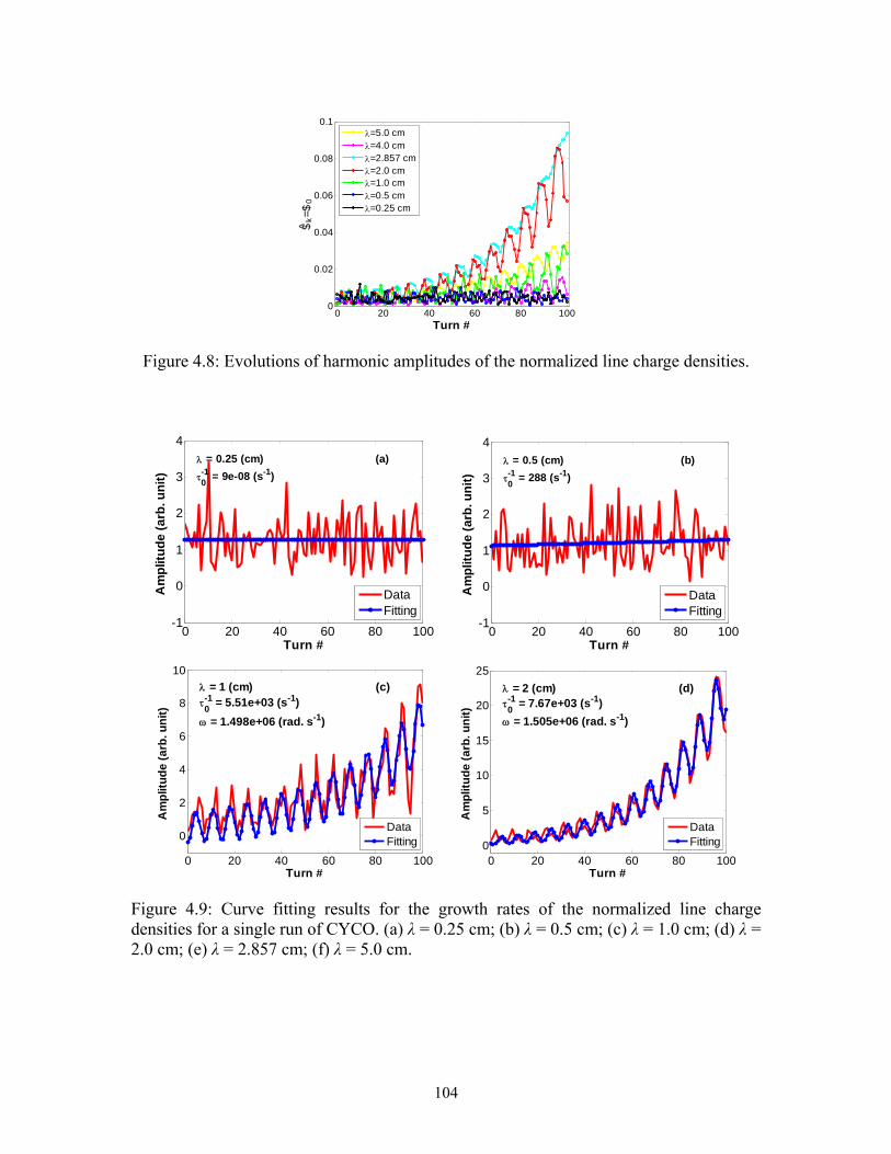
104
Figure 4.8: Evolutions of harmonic amplitudes of the normalized line charge densities.
Figure 4.9: Curve fitting results for the growth rates of the normalized line charge densities for a single run of CYCO. (a) λ = 0.25 cm; (b) λ = 0.5 cm; (c) λ = 1.0 cm; (d) λ = 2.0 cm; (e) λ = 2.857 cm; (f) λ = 5.0 cm.
0 20 40 60 80 1000
0.02
0.04
0.06
0.08
0.1
Turn #
$k=$
0
=5.0 cm=4.0 cm=2.857 cm=2.0 cm=1.0 cm=0.5 cm=0.25 cm
0 20 40 60 80 100-1
0
1
2
3
4
Turn #
Am
plit
ud
e (
arb
. un
it)
= 0.25 (cm) (a)
-10
= 9e-08 (s-1)
DataFitting
0 20 40 60 80 100-1
0
1
2
3
4
Turn #
Am
plit
ud
e (
arb
. un
it)
= 0.5 (cm) (b)
-10
= 288 (s-1)
DataFitting
0 20 40 60 80 100
0
2
4
6
8
10
Turn #
Am
plit
ud
e (
arb
. un
it)
= 1 (cm) (c)-10
= 5.51e+03 (s-1)
= 1.498e+06 (rad. s-1)
DataFitting
0 20 40 60 80 1000
5
10
15
20
25
Turn #
Am
plit
ud
e (
arb
. un
it)
= 2 (cm) (d)-1
0 = 7.67e+03 (s-1)
= 1.505e+06 (rad. s-1)
DataFitting
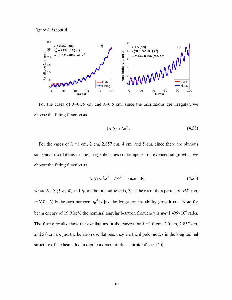
105
Figure 4.9 (cont’d)
For the cases of l=0.25 cm and l=0.5 cm, since the oscillations are irregular, we
choose the fitting function as
.ˆ|)(|0
1
t
et (4.55)
For the cases of l =1 cm, 2 cm, 2.857 cm, 4 cm, and 5 cm, since there are obvious
sinusoidal oscillations in line charge densities superimposed on exponential growths, we
choose the fitting function as
),cos(ˆ|)(| 00 /
1 tPeet TQt
t
(4.56)
where , P, Q, , , and 0 are the fit coefficients, T0 is the revolution period of ion,
t=NtT0, Nt is the turn number, 0-1 is just the long-term instability growth rate. Note for
beam energy of 19.9 keV, the nominal angular betatron frequency is =1.499106 rad/s.
The fitting results show the oscillations in the curves for l =1.0 cm, 2.0 cm, 2.857 cm,
and 5.0 cm are just the betatron oscillations, they are the dipole modes in the longitudinal
structure of the beam due to dipole moment of the centroid offsets [20].
0 20 40 60 80 1000
5
10
15
20
25
30
Turn #
Am
plit
ud
e (
arb
. un
it)
= 2.857 (cm) (e)
-10
= 7.22e+03 (s-1)
= 1.501e+06 (rad. s-1)
DataFitting
0 20 40 60 80 100
0
2
4
6
8
10
Turn #
Am
plit
ud
e (
arb
. un
it)
= 5 (cm) (f)-1
0 = 5.74e+03 (s-1)
= 1.504e+06 (rad. s-1)
DataFitting
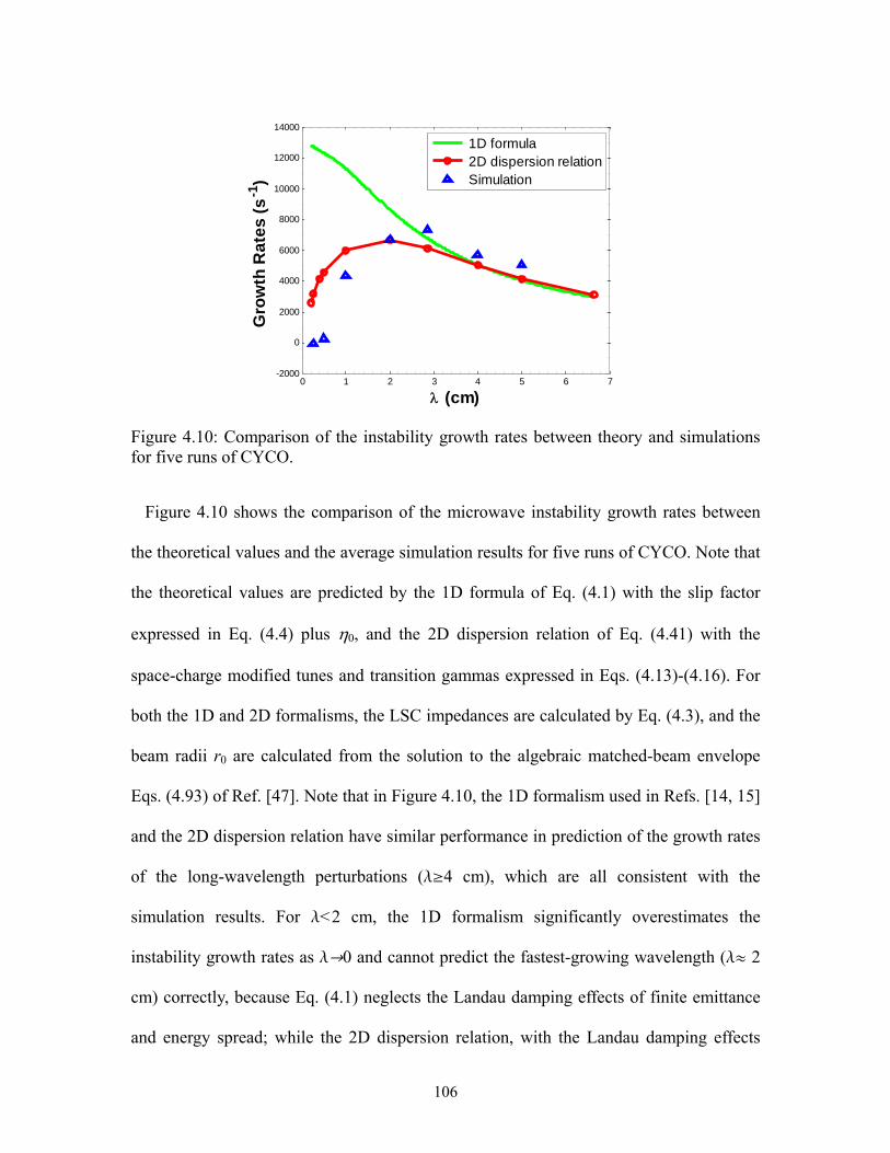
106
Figure 4.10: Comparison of the instability growth rates between theory and simulations for five runs of CYCO.
Figure 4.10 shows the comparison of the microwave instability growth rates between
the theoretical values and the average simulation results for five runs of CYCO. Note that
the theoretical values are predicted by the 1D formula of Eq. (4.1) with the slip factor
expressed in Eq. (4.4) plus 0, and the 2D dispersion relation of Eq. (4.41) with the
space-charge modified tunes and transition gammas expressed in Eqs. (4.13)-(4.16). For
both the 1D and 2D formalisms, the LSC impedances are calculated by Eq. (4.3), and the
beam radii r0 are calculated from the solution to the algebraic matched-beam envelope
Eqs. (4.93) of Ref. [47]. Note that in Figure 4.10, the 1D formalism used in Refs. [14, 15]
and the 2D dispersion relation have similar performance in prediction of the growth rates
of the long-wavelength perturbations (l¥4 cm), which are all consistent with the
simulation results. For l<2 cm, the 1D formalism significantly overestimates the
instability growth rates as lØ0 and cannot predict the fastest-growing wavelength (lº 2
cm) correctly, because Eq. (4.1) neglects the Landau damping effects of finite emittance
and energy spread; while the 2D dispersion relation, with the Landau damping effects
0 1 2 3 4 5 6 7-2000
0
2000
4000
6000
8000
10000
12000
14000
(cm)
Gro
wth
Ra
tes
(s
-1)
1D formula 2D dispersion relation Simulation

107
taken into account, has a much better performance than the conventional 1D formula in
prediction of instability growth rates in the short-wavelength limits (l<2 cm) and the
fastest-growing wavelength, though there still exist some bigger discrepancies between
the simulations and theory for very short wavelength l<1 cm. Therefore we can see the
Landau damping is a necessary mechanism to explain the low instability growth rates of
the short-wavelength perturbations ( is less than or comparable to r0), which cannot be
explained by the conventional 1D formalisms. Only at larger wavelengths ( >> r0) will
the 1D and 2D dispersion relations have the similar performance.
4.4.2 Growth rates of instability with variable beam intensities
In order to study the dependence of microwave instability growth rates on initial beam
intensities, simulations using CYCO are carried out for SIR beams with Ek0 = 19.9 keV,
sE= 0 eV, b = 300 ns (Lb 40 cm), x,0=y,0=50p mm mrad, I0 =0.1, 0.3, 0.5, 5.0, and 20
mA, respectively. The initial distributions are uniform in both the 4-D transverse phase
space (x, x£, y, y£) and the longitudinal charge density. The simulation for each intensity
level is performed five times using five different initial micro-distributions, and the
average simulated growth rates of the selected perturbation wavelengths of the five runs
are used in analysis. For I0 >20 mA, due to fast development of beam instability, the beam
dynamics may enter the nonlinear regime only after several turns of coasting. This makes
the fitting work difficult and inaccurate, therefore the simulation results for the intensities
of I0 >20 mA are not available in this paper.
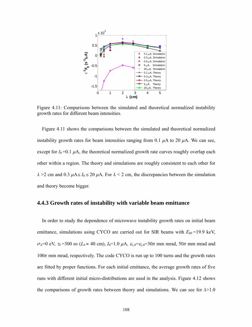
108
Figure 4.11: Comparisons between the simulated and theoretical normalized instability growth rates for different beam intensities.
Figure 4.11 shows the comparisons between the simulated and theoretical normalized
instability growth rates for beam intensities ranging from 0.1 mA to 20 mA. We can see,
except for I0 =0.1 mA, the theoretical normalized growth rate curves roughly overlap each
other within a region. The theory and simulations are roughly consistent to each other for
l >2 cm and 0.3 mA§ I0 § 20 mA. For l < 2 cm, the discrepancies between the simulation
and theory become bigger.
4.4.3 Growth rates of instability with variable beam emittance
In order to study the dependence of microwave instability growth rates on initial beam
emittance, simulations using CYCO are carried out for SIR beams with Ek0 =19.9 keV,
sE=0 eV, b =300 ns (Lb 40 cm), I0=1.0 mA, x,0=y,0=30p mm mrad, 50p mm mrad and
100p mm mrad, respectively. The code CYCO is run up to 100 turns and the growth rates
are fitted by proper functions. For each initial emittance, the average growth rates of five
runs with different initial micro-distributions are used in the analysis. Figure 4.12 shows
the comparisons of growth rates between theory and simulations. We can see for l>1.0
0 1 2 3 4 5
-1.5
-1
-0.5
0
0.5
1x 10
4
(cm)
-1/I 0 (
s-1
/ A
)
0.1 A, Simulation 0.3 A, Simulation
0.5 A, Simulation
5 A, Simulation
20 A, Simulation 0.1 A, Theory
0.3 A, Theory
0.5 A, Theory
5 A, Theory 20 A, Theory

109
cm, the simulated and theoretical instability growth rates are consistent with each other,
the larger emittance may help to suppress the instability growth rates. While for l<1.0 cm,
the discrepancies between the simulation and theory become bigger.
Figure 4.12: Comparisons of microwave instability growth rates between theory and simulations for variable initial emittance.
4.4.4 Growth rates of instability with variable beam energy spread
Figure 4.13 shows the comparisons of growth rates between theory and simulations for
SIR beams with Ek0=19.9 keV, b =300 ns (Lb 40 cm), I0 =1.0 mA, x,0=y,0=50 mm mrad,
sE=0, 50, and 75 eV, respectively. The code CYCO is run up to 100 turns and the growth
rates are fitted by proper functions. For each initial RMS energy spread sE, the average
growth rates of five runs with different initial micro-distributions are used in the analysis.
We can see for l>2.0 cm, the simulated and theoretical instability growth rates are
consistent with each other, the larger energy spread may help to suppress the instability
growth rates. While for l<2.0 cm, the discrepancies between the simulation and theory
become bigger.
0 1 2 3 4 50
0.5
1
1.5
2
x 104
(cm)
-1 (
s-1
)
30 mm mrad, Simulaion 50 mm mrad, Simulaion 100 mm mrad, Simulaion 30 mm mrad, Theory 50 mm mrad, Theory 100 mm mrad, Theory
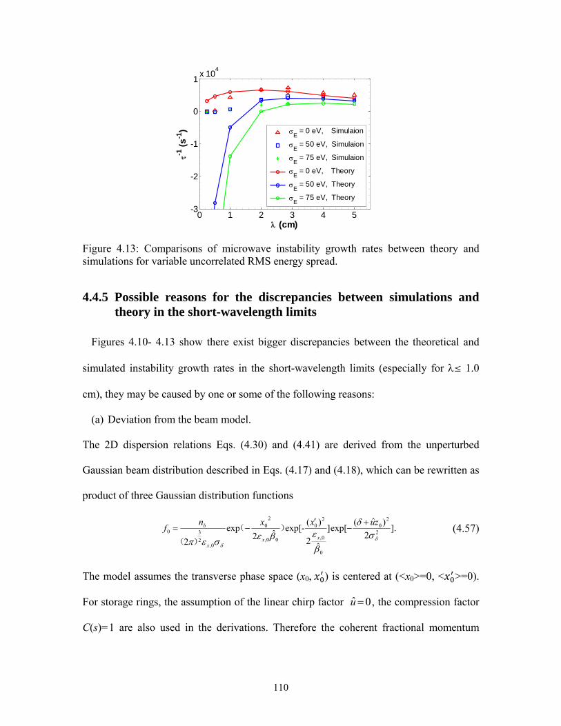
110
Figure 4.13: Comparisons of microwave instability growth rates between theory and simulations for variable uncorrelated RMS energy spread.
4.4.5 Possible reasons for the discrepancies between simulations and theory in the short-wavelength limits
Figures 4.10- 4.13 show there exist bigger discrepancies between the theoretical and
simulated instability growth rates in the short-wavelength limits (especially for § 1.0
cm), they may be caused by one or some of the following reasons:
(a) Deviation from the beam model.
The 2D dispersion relations Eqs. (4.30) and (4.41) are derived from the unperturbed
Gaussian beam distribution described in Eqs. (4.17) and (4.18), which can be rewritten as
product of three Gaussian distribution functions
].2
)ˆ(exp[]
ˆ2
)(-exp[
ˆ2exp
22
20
0
0,
20
00,
20
0,2
30
zuxxnf
xxx
b
)(
)( (4.57)
The model assumes the transverse phase space (x0, ) is centered at (<x0>=0, < >=0).
For storage rings, the assumption of the linear chirp factor 0ˆ u , the compression factor
C(s)=1 are also used in the derivations. Therefore the coherent fractional momentum
0 1 2 3 4 5-3
-2
-1
0
1x 10
4
(cm)
-1 (
s-1
)
E = 0 eV, Simulaion
E = 50 eV, Simulaion
E = 75 eV, Simulaion
E = 0 eV, Theory
E = 50 eV, Theory
E = 75 eV, Theory

111
deviation ,0ˆ 00 zu and there is no correlation between the transverse
and longitudinal distributions. The initial unperturbed distribution function described in
Eq. (4.57) is just the product of three normal distribution functions with zero-mean.
While as the beam coasts in the ring, there will be local centroid offset <x0> induced by
the coherent fractional momentum deviation <d0> due to dispersion function D:
.D 00 x (4.58)
In addition, when sinusoidal centroid wiggling takes place due to space charge force, the
correlated fractional moment deviation 0ˆzu should be replaced by a sinusoidal function
of z0, then the compression factor C(s)∫1 and will be dependent on s or t. The non-zero
<x0>, <d0> and non-constant, s-dependent compression factor C(s) will shift the centers
of beam distributions in the longitudinal and transverse phase space, produce a
radial-longitudinal correlation in distribution function. Consequently, the 2D dispersion
relations (4.30) and (4.41) will be modified, the amplitude of perturbed harmonic line
density |)(||),(| ,1 tgtzn kk described in Eq. (4.34) should be replaced by
|)()(||),(| ,1 tgtCtzn kk too. This may cause the bigger discrepancies between the
theoretical and simulated instability growth rates in the short-wavelength limits.
(b) Curvature effects
The LSC impedance, space-charge modified betatron tunes and transition gammas
are all derived for an infinite long, straight beam model, while the SIR consists of four
90o bending magnets which account for about 43% of the ring circumference. When the
beam enters these bends, the curvature effects on the longitudinal and transverse beam
dynamics are not taken into account in the theoretical analysis.
(c) LSC fields of the dipole mode
112
The centroid wiggling may induce the LSC fields of the dipole mode which are
neglected in the theoretical analysis.
(d) Spectral leakages
In the data analysis, the line charge density perturbations around the fastest-growing
wavelength (2.0 cm) have larger amplitudes comparing to the modes with smaller
growth rates, and the FFT analysis is applied to a bunch with finite length using
rectangular window. The fastest-growing modes may inevitably create the new frequency
components (false spectrum) spreading in the whole frequency domain, namely, the
so-called spectral leakages. The leaked spectra from the faster-growing modes may mix
with and mask the real spectra of the slower-growing modes, therefore lower the
resolutions of the FFT analysis results.
(e) Initial distribution
In Figures 4.12 and 4.13, because the beams with uniform longitudinal charge density
are used in the simulations, their residual line charge modulation amplitudes are
vanishingly small (theoretically speaking, they should be 0 in ideal conditions). When the
growth rates in short-wavelength limits are negative due to larger beam emittance and
energy spread, they can hardly be detected since the initial density modulation amplitudes
have reached minima already.
In summary, the bigger discrepancies between the theoretical and simulated instability
growth rates in the short-wavelength limits may be caused by various reasons. Due to
complexity of the problem, for the time being, further discussions are not available in this
dissertation.
113
4.5 Conclusions
Due to space charge effects and radial-longitudinal coupling, an ideally isochronous
ring becomes a quasi-isochronous ring, which may result in the microwave instability and
a finite revolution frequency spread. The relative motions among particles along the
azimuthal direction are not frozen completely. The Landau damping mechanism still
takes effect and may suppress the microwave instability in the isochronous regime.
A modified 2D dispersion relation is introduced to discuss the Landau damping effects
for a coasting beam in the isochronous regime. The radial-longitudinal coupling transfer
matrix elements R51 and R52 are included in the 2D dispersion relation. These elements
can modify the coherent slip factor, together with R56, they also provide an exponential
suppression for the instability growth rates of a beam with finite energy spread and
emittance by Landau damping effects. The 2D dispersion relation is benchmarked by
simulation code CYCO for bunches with variable initial beam intensities, energy spread
and emittance. The theory agrees well with the numerical simulations for perturbation
wavelengths of l>2.0 cm. While for l<2.0 cm, the discrepancies between simulations
and theoretical predictions become larger. The possible reasons for the discrepancies are
pointed out and discussed. By comparisons, the 2D dispersion relation has a better
performance than the conventional 1D growth rate formula; the latter significantly
overestimates the growth rates in the short–wavelength limit lØ0 and is incapable of
predicting the correct fastest-growing wavelength.
In summary, the Landau damping effect is a necessary and important mechanism for an
accurate prediction of the instability growth rates of the short-wavelength perturbations
and the fastest-growing wavelength.
114
Chapter 5
DESIGN AND TEST OF ENERGY ANALYZER3
5.1 Introduction
Due to the repulsive space charge force, an initially monoenergetic bunch will develop
energy spread among the beam particles when the bunch coasts in a storage ring. For the
evolutions of the microwave instability and beam distribution, the development of the
energy spread plays an important role and need to be measured accurately. For this
purpose, SIR Lab has constructed a compact, high resolution electrostatic retarding field
energy analyzer (RFA) with rectangular electrodes and a large entrance slit. This chapter
will present the design and test of the energy analyzer.
5.2 Working principles and design considerations of the RFA
Because of the simple structure and high signal-to-noise ratios, an electrostatic RFA
was chosen as the energy measurement device for the low energy SIR beam. The working
principles of the generic electrostatic RFAs are simple: there is an electrode biased to a
variable retarding voltage inside the analyzer (see Figure 5.1(a)), if the longitudinal
component of the kinetic energy of an incident particle is no less than the peak of the
retarding potential barrier, the particle can overcome the barrier and reach the current
collector to form collector current. The energy profiles within the beam can be deciphered
by analyzing the collector current as a function of the scanning retarding voltages V1.
3 The contents related to design and testing of energy analyzer of this chapter is written based on Ref. [19].

There
for e
which
Figurwith slopeelectr[48])
In
effect
(a)
Le
charg
differ
of the
to the
after
the ap
This
e are severa
example, the
h Ref. [48] p
re 5.1: (a) ScV2=V0 for m
e between V=ron emission.
n the design
ts which ma
) Aperture le
t us assume
ge and kineti
rent field str
e aperture ar
e aperture ax
the aperture
perture, the
aperture len
l types of R
e parallel-pl
provided an
chematic of monoenerget=V0-DV and n is shown in
n and operat
y affect its r
ns effect
e a beam en
ic energy of
engths befor
re bent towar
xis sees a ra
e. Since the p
net effect is
ns effect can b
RFA which a
late analyze
excellent rev
a basic paratic particlesV=V0 is due
n the dotted
tion of a RF
resolution.
nters a decel
a single bea
re and after t
rds the apert
dial focusing
particle’s ene
defocusing
be character
115
are commonl
er, spherical
view.
allel-plate RF (c) Usual e to the trajecurve. (Not
FA, special
lerating field
am particle a
the aperture,
ture. The par
g force befo
ergy after th
resulting in
rized by a foc
ly used in th
condenser,
RFA. (b) IdeaI-V characte
ectory effectte: the figure
attention ne
d through a
are e and eV0
, the electric
rticle with a
ore the apertu
he aperture is
n an increase
cal power [4
he energy m
Faraday ca
al I-V characeristic cutoft. The effect e is reproduc
eeds to be p
an entrance a
V0, respective
c field lines i
radial offse
ure and a de
s smaller tha
e of the dive
48] as
measurement
age, etc., fo
cteristic curvff curve. Th of secondarced from Re
paid to som
aperture. Th
ely. Due to th
in the vicinit
t with respec
efocusing on
an that befor
ergence angl
ts,
or
ve he ry ef.
me
he
he
ty
ct
ne
re
e.

116
,4/)(/1 012 VEEf (5.1)
where E1 and E2 are the field strength before and after the entrance aperture. Ref. [47]
provides a detailed derivation for Eq. (5.1).
(b) Trajectory effect
Only the longitudinal component of the kinetic energy is effective to overcome the
retarding potential. For example, among the existing analyzers, the simplest one is the
primitive two-element parallel-plate analyzer (see Figure 5.1(a)). This type of RFA has a
good resolution only when the trajectories of the beam are parallel to the analyzer axis. In
this case, for a monoenergetic beam with initial kinetic energy eV0, the ideal I-V (current
signal v.s regarding voltage) characteristic curve of the analyzer is similar to a step
function with a sharp cutoff at V2=V0 (see Figure 5.1(b)). In reality, due to the initial beam
emittance, the aperture lens effect, space charge effect and misalignment, the moving
directions of the particles inside the analyzer usually have finite nonzero slopes with
respect to the analyzer axis. Then the actual I-V curve for a monoenergetic beam may
look like that in Figure 5.1(c), where the curve begins to drop at V=V0-DV. This may
result in a poor resolution of the parallel-plate analyzer DV/V0 typically in the range of
10-3-10-2. In order to suppress this trajectory effect and expansion of beamlet due to space
charge effect, a focusing electrode is usually introduced in the analyzer between the
entrance aperture and the retarding electrode; another option is to choose a special
multifunctional retarding/focusing electrode that can decelerate and focus the sampled
beamlet at the same time.
(c) Secondary electron emission
When the charged particles bombard the metal current collector, a fraction of the
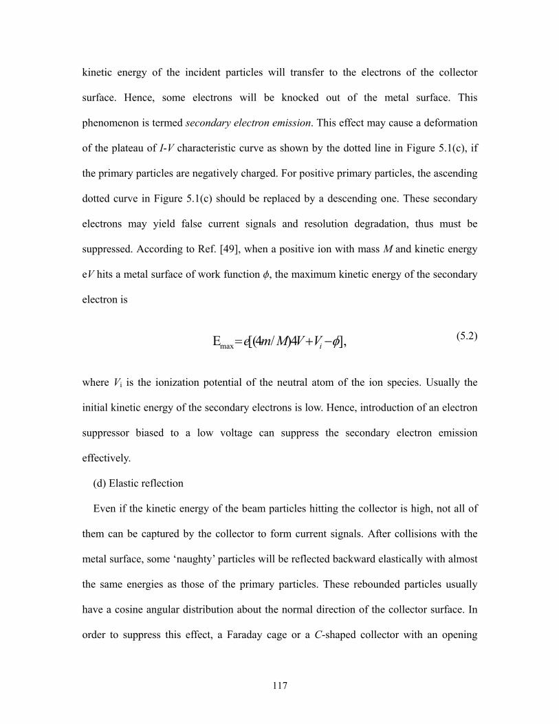
117
kinetic energy of the incident particles will transfer to the electrons of the collector
surface. Hence, some electrons will be knocked out of the metal surface. This
phenomenon is termed secondary electron emission. This effect may cause a deformation
of the plateau of I-V characteristic curve as shown by the dotted line in Figure 5.1(c), if
the primary particles are negatively charged. For positive primary particles, the ascending
dotted curve in Figure 5.1(c) should be replaced by a descending one. These secondary
electrons may yield false current signals and resolution degradation, thus must be
suppressed. According to Ref. [49], when a positive ion with mass M and kinetic energy
eV hits a metal surface of work function f, the maximum kinetic energy of the secondary
electron is
],4)/4[(Emax iVVMme (5.2)
where Vi is the ionization potential of the neutral atom of the ion species. Usually the
initial kinetic energy of the secondary electrons is low. Hence, introduction of an electron
suppressor biased to a low voltage can suppress the secondary electron emission
effectively.
(d) Elastic reflection
Even if the kinetic energy of the beam particles hitting the collector is high, not all of
them can be captured by the collector to form current signals. After collisions with the
metal surface, some ‘naughty’ particles will be reflected backward elastically with almost
the same energies as those of the primary particles. These rebounded particles usually
have a cosine angular distribution about the normal direction of the collector surface. In
order to suppress this effect, a Faraday cage or a C-shaped collector with an opening
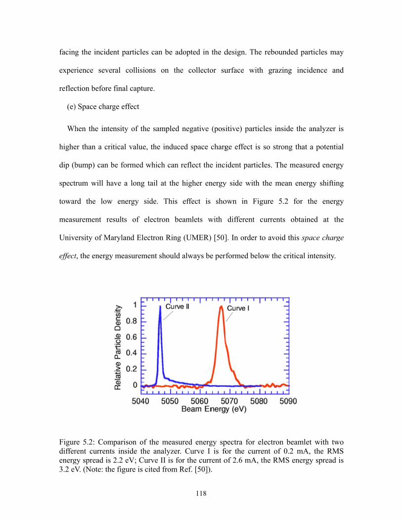
facing
exper
reflec
(e)
Wh
highe
dip (b
spect
towar
meas
Univ
effect
Figurdifferenerg3.2 eV
g the incide
rience sever
ction before
) Space charg
hen the inte
er than a crit
bump) can b
trum will ha
rd the low
urement re
ersity of Ma
t, the energy
re 5.2: Comrent currentsgy spread is V. (Note: the
ent particles
ral collision
final capture
ge effect
nsity of the
tical value,
be formed w
ave a long ta
energy sid
sults of ele
aryland Elec
y measureme
mparison of ts inside the 2.2 eV; Cure figure is ci
can be adop
ns on the
e.
sampled ne
the induced
which can ref
ail at the hi
de. This ef
ectron beam
tron Ring (U
ent should alw
the measureanalyzer. C
rve II is for tted from Re
118
pted in the d
collector su
egative (posi
space charg
flect the inci
gher energy
ffect is sho
mlets with
UMER) [50]
ways be per
ed energy spCurve I is fothe current of. [50]).
design. The
urface with
itive) particl
ge effect is
ident particl
y side with t
own in Fig
different c
]. In order to
formed belo
pectra for elfor the curreof 2.6 mA, th
rebounded p
h grazing in
les inside th
so strong th
les. The mea
the mean en
gure 5.2 for
urrents obt
o avoid this
ow the critica
lectron beament of 0.2 mhe RMS ene
particles ma
ncidence an
he analyzer
hat a potentia
asured energ
nergy shiftin
r the energ
ained at th
space charg
al intensity.
mlet with twmA, the RMergy spread
ay
nd
is
al
gy
ng
gy
he
ge
wo MS
is
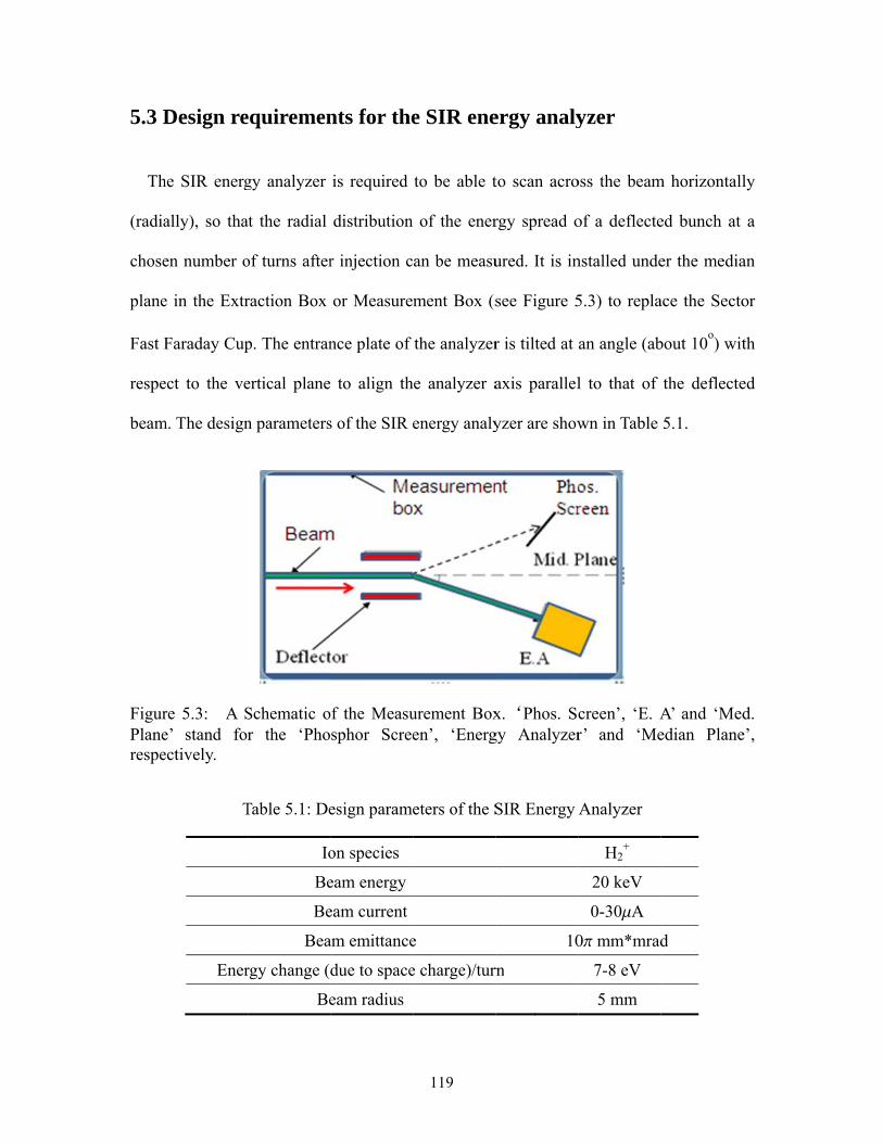
5.3 D
Th
(radia
chose
plane
Fast F
respe
beam
FigurPlanerespe
Design re
he SIR energ
ally), so tha
en number o
e in the Extr
Faraday Cup
ect to the ve
m. The design
re 5.3: A Se’ stand forectively.
T
Ener
equiremen
gy analyzer
at the radial
of turns after
raction Box
p. The entran
ertical plane
n parameters
Schematic or the ‘Pho
Table 5.1: De
Io
Be
Be
Bea
rgy change (
Be
nts for the
is required
distribution
r injection c
or Measure
nce plate of
to align th
s of the SIR e
of the Measusphor Scree
esign parame
on species
eam energy
eam current
am emittance
due to space
eam radius
119
e SIR ene
to be able t
of the ener
an be measu
ment Box (s
the analyzer
he analyzer a
energy analy
urement Boxen’, ‘Energ
eters of the S
e
e charge)/tur
ergy analy
to scan acro
rgy spread o
ured. It is in
see Figure 5
r is tilted at
axis parallel
yzer are show
x.‘Phos. Scgy Analyzer
SIR Energy
10
rn
yzer
oss the beam
of a deflecte
nstalled unde
5.3) to repla
an angle (ab
l to that of
wn in Table
creen’, ‘E. Ar’ and ‘Me
Analyzer
H2+
20 keV
0-30mA
0p mm*mrad
7-8 eV
5 mm
m horizontall
ed bunch at
er the media
ace the Secto
bout 10o) wit
the deflecte
5.1.
A’ and ‘Mededian Plane
d
ly
a
an
or
th
ed
d. e’,

FigurexpanThe athe m
Fig
expan
show
spatia
follow
beam
10 mA
possi
entran
large
5.4 A
Th
resolu
re 5.4: A snded beam. analyzer can
middle of the
gure 5.4 dep
nded beam (
wn in the plot
al relation b
w behind the
m size of SIR
A level (out
ble, we ado
nce aperture
entrance ap
A brief in
he University
ution cylindr
schematic oThe beam (g
n scan back aanalyzer de
picts the sch
(green oval)
t. The beam
between the
e beam and
R is about 10
side the ana
opted a 14 m
e instead of
erture make
ntroductio
y of Maryla
rical RFAs t
f the SIR green oval) and forth alo
epicts a samp
ematic of th
) due to spa
is moving in
energy ana
watch along
0 mm in diam
alyzer for a D
mm (vertica
f a conventi
s the design
on to the U
and has desi
o measure th
120
energy analis moving toong the ringpled beam sl
he SIR energ
ace charge e
nto the pape
alyzer and th
g its moving
meter and th
DC beam). I
al) μ 1 mm
onal small
work more
UMER an
igned the 2n
he energy sp
lyzer with owards the a
g radius. Thelice or beaml
gy analyzer.
effect and di
er. This figur
he beam in
g direction to
e beam peak
In order to s
m (horizonta
hole (Figure
challenging
nalyzer
nd and 3rd g
pread of the e
a horizontaanalyzer (ine thin yellowlet.
A horizonta
ispersion fun
re shows a sc
the measur
owards the
k current is o
sample as m
al) rectangul
e 5.4). This
.
generation c
electron bea
ally (radiallynto the paperw rectangle i
ally (radially
nction is als
cenario of th
rement, if w
analyzer. Th
only on abou
much beam a
lar slit as th
s asymmetri
ompact, hig
m in UMER
y) r). in
y)
so
he
we
he
ut
as
he
c,
gh
R.
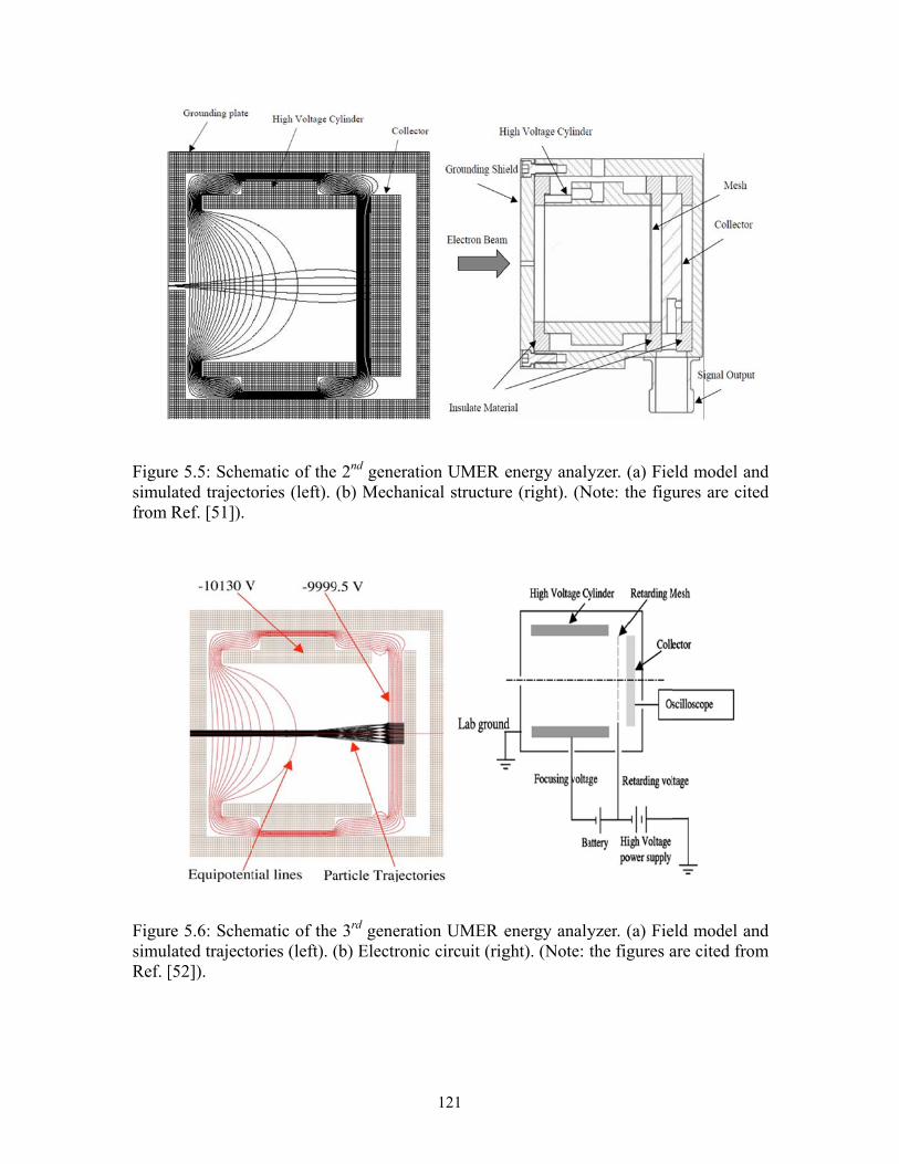
Figursimulfrom
FigursimulRef. [
re 5.5: Schemlated trajectoRef. [51]).
re 5.6: Schemlated trajecto[52]).
matic of theories (left).
matic of theories (left). (
2nd generati(b) Mechani
e 3rd generati(b) Electroni
121
ion UMER ical structur
ion UMER eic circuit (rig
energy analyre (right). (N
energy analyght). (Note:
yzer. (a) FieNote: the figu
yzer. (a) Fiethe figures a
eld model anures are cite
eld model anare cited from
nd ed
nd m
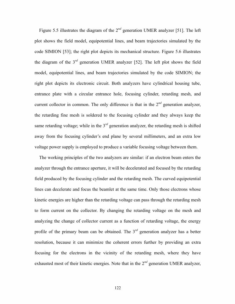
122
Figure 5.5 illustrates the diagram of the 2nd generation UMER analyzer [51]. The left
plot shows the field model, equipotential lines, and beam trajectories simulated by the
code SIMION [53]; the right plot depicts its mechanical structure. Figure 5.6 illustrates
the diagram of the 3rd generation UMER analyzer [52]. The left plot shows the field
model, equipotential lines, and beam trajectories simulated by the code SIMION; the
right plot depicts its electronic circuit. Both analyzers have cylindrical housing tube,
entrance plate with a circular entrance hole, focusing cylinder, retarding mesh, and
current collector in common. The only difference is that in the 2nd generation analyzer,
the retarding fine mesh is soldered to the focusing cylinder and they always keep the
same retarding voltage; while in the 3rd generation analyzer, the retarding mesh is shifted
away from the focusing cylinder’s end plane by several millimeters, and an extra low
voltage power supply is employed to produce a variable focusing voltage between them.
The working principles of the two analyzers are similar: if an electron beam enters the
analyzer through the entrance aperture, it will be decelerated and focused by the retarding
field produced by the focusing cylinder and the retarding mesh. The curved equipotential
lines can decelerate and focus the beamlet at the same time. Only those electrons whose
kinetic energies are higher than the retarding voltage can pass through the retarding mesh
to form current on the collector. By changing the retarding voltage on the mesh and
analyzing the change of collector current as a function of retarding voltage, the energy
profile of the primary beam can be obtained. The 3rd generation analyzer has a better
resolution, because it can minimize the coherent errors further by providing an extra
focusing for the electrons in the vicinity of the retarding mesh, where they have
exhausted most of their kinetic energies. Note that in the 2nd generation UMER analyzer,
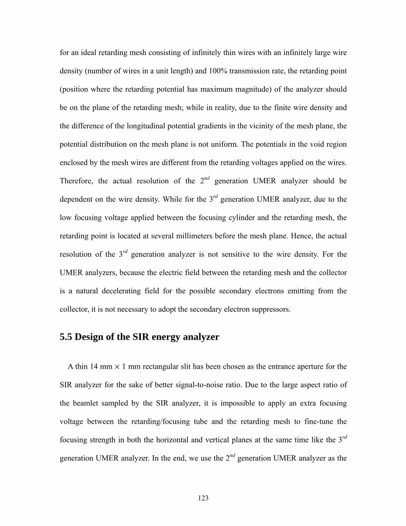
123
for an ideal retarding mesh consisting of infinitely thin wires with an infinitely large wire
density (number of wires in a unit length) and 100% transmission rate, the retarding point
(position where the retarding potential has maximum magnitude) of the analyzer should
be on the plane of the retarding mesh; while in reality, due to the finite wire density and
the difference of the longitudinal potential gradients in the vicinity of the mesh plane, the
potential distribution on the mesh plane is not uniform. The potentials in the void region
enclosed by the mesh wires are different from the retarding voltages applied on the wires.
Therefore, the actual resolution of the 2nd generation UMER analyzer should be
dependent on the wire density. While for the 3rd generation UMER analyzer, due to the
low focusing voltage applied between the focusing cylinder and the retarding mesh, the
retarding point is located at several millimeters before the mesh plane. Hence, the actual
resolution of the 3rd generation analyzer is not sensitive to the wire density. For the
UMER analyzers, because the electric field between the retarding mesh and the collector
is a natural decelerating field for the possible secondary electrons emitting from the
collector, it is not necessary to adopt the secondary electron suppressors.
5.5 Design of the SIR energy analyzer
A thin 14 mm μ 1 mm rectangular slit has been chosen as the entrance aperture for the
SIR analyzer for the sake of better signal-to-noise ratio. Due to the large aspect ratio of
the beamlet sampled by the SIR analyzer, it is impossible to apply an extra focusing
voltage between the retarding/focusing tube and the retarding mesh to fine-tune the
focusing strength in both the horizontal and vertical planes at the same time like the 3rd
generation UMER analyzer. In the end, we use the 2nd generation UMER analyzer as the

124
main design reference for the SIR analyzer.
From emittance measurement, the divergence angles of the primary SIR beam in the
horizontal and vertical planes are found to be roughly the same. In order to focus the
particles at the edges of the sampled beamlet inside the analyzer with the same focusing
strength in both planes for optimum resolution, the contour of the equipotential lines in
any planes normal to the analyzer axis must be a family of concentric rectangles, of
which the aspect ratios should be similar to that of the sampled beamlet in the
retarding/focusing region. This requires both the retarding/focusing electrodes and the
housing of SIR analyzer must have rectangular cross-section.
Due to the much higher particle energy (which is equal to the retarding/focusing
voltage times unit charge), and the much larger vertical dimensions of the beamlet
sampled by the SIR analyzer than those of the electron beamlet sampled by the UMER
analyzer, the distance between the retarding mesh and the entrance plate of the SIR
analyzer must be much shorter than that of the UMER analyzer to get a proper focusing
for the SIR beamlet, otherwise the particles will be over-focused yielding poor resolution.
In addition, in the SIR analyzer, since the electric field between the retarding mesh and
the collector is an accelerating field for the possible secondary electrons escaping from
the collector surface, a secondary electron suppressor which is biased to a negative
voltage should be introduced between the retarding mesh and the collector. For the above
reasons, the longitudinal potential gradient between the retarding mesh and entrance plate
of the SIR analyzer is much higher than that of the UMER analyzer, especially in the
vicinity of the retarding mesh plane. This makes the resulting analyzer resolution highly
dependent on the mesh wire density. Considering both the transmission rates and wire
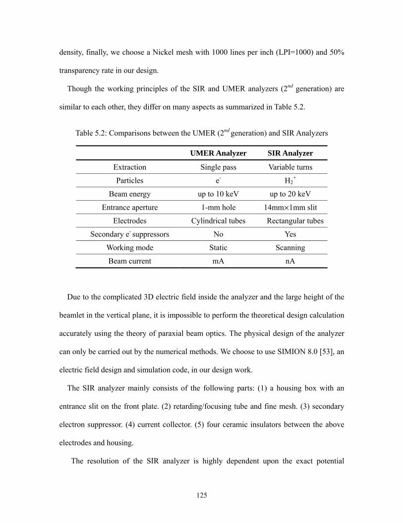
125
density, finally, we choose a Nickel mesh with 1000 lines per inch (LPI=1000) and 50%
transparency rate in our design.
Though the working principles of the SIR and UMER analyzers (2nd generation) are
similar to each other, they differ on many aspects as summarized in Table 5.2.
Table 5.2: Comparisons between the UMER (2nd generation) and SIR Analyzers
UMER Analyzer SIR Analyzer
Extraction Single pass Variable turns
Particles e- H2+
Beam energy up to 10 keV up to 20 keV
Entrance aperture 1-mm hole 14mmμ1mm slit
Electrodes Cylindrical tubes Rectangular tubes
Secondary e- suppressors No Yes
Working mode Static Scanning
Beam current mA nA
Due to the complicated 3D electric field inside the analyzer and the large height of the
beamlet in the vertical plane, it is impossible to perform the theoretical design calculation
accurately using the theory of paraxial beam optics. The physical design of the analyzer
can only be carried out by the numerical methods. We choose to use SIMION 8.0 [53], an
electric field design and simulation code, in our design work.
The SIR analyzer mainly consists of the following parts: (1) a housing box with an
entrance slit on the front plate. (2) retarding/focusing tube and fine mesh. (3) secondary
electron suppressor. (4) current collector. (5) four ceramic insulators between the above
electrodes and housing.
The resolution of the SIR analyzer is highly dependent upon the exact potential

distri
wire
mode
deal w
up as
Figur(right
Th
betwe
plane
retard
progr
impac
thoug
simul
mesh
bution on an
density. Bec
el containing
with this pro
s shown in th
re 5.7: The t).
he small me
een two pla
e boundaries
ding mesh p
ramming la
ction point
gh the small
lation, a gro
h sample mo
nd near the
cause of the
g all the wire
oblem, a sma
he left plot o
movable sm
esh model c
ane boundar
s are separa
plane at a d
anguage Lua
and move t
l mesh mode
oup of ions
ves along th
retarding m
high calcula
es of the ent
all sample o
f Figure 5.7.
mall mesh m
consists of
ries with pro
ated by a s
distance whi
a [54] emb
the small m
el containing
are shot tow
he whole ret
126
esh plane, w
ation worklo
tire piece of
of the real m
.
model (left)
eight cross
oper potenti
short distanc
ch is close
bedded in
mesh model
g an accurat
wards the ret
arding plane
which is non
oad, it is imp
f retarding m
mesh model w
) and simul
sing wire se
ials calculat
ce d. When
to d/2, a sh
SIMION ca
there, so th
te field distr
tarding mes
e back and f
nuniform due
possible to s
mesh in the s
with high res
lated particl
egments pla
ted in advan
n an ion ap
hort script w
an predict
hat the parti
ribution. In
h one by on
forth, so that
e to the finit
set up a mes
imulation. T
solution is se
le trajectorie
aced midwa
nce. The tw
pproaches th
written in th
the possibl
icle can pas
the trajector
ne. The sma
t the particle
te
sh
To
et
es
ay
wo
he
he
le
ss
ry
all
es
can p
the w
Figurby SIsuppr
Th
some
pass through
whole real me
re 5.8: Two sIMIOM, wheressor are Vr
he electrodes
e typical ions
it one by on
esh can be si
schematics oere the beamretarding=20 kV
s, equipoten
s in the SIR
ne (right plot
imulated wit
of the SIR enm energy is 2V and Vsuppre
ntial lines (g
analyzer sim
127
t of Figure 5
th a good res
nergy analyz20.01 keV, thessor=-300V, r
green lines),
mulated by S
5.7). By this
solution.
zer and partihe voltages orespectively
and the traj
IMION are
way, the traj
icle trajectorof the regardy.
ajectories (bl
shown in Fi
ajectories nea
ries simulateding mesh an
lack lines) o
gure 5.8.
ar
ed nd
of
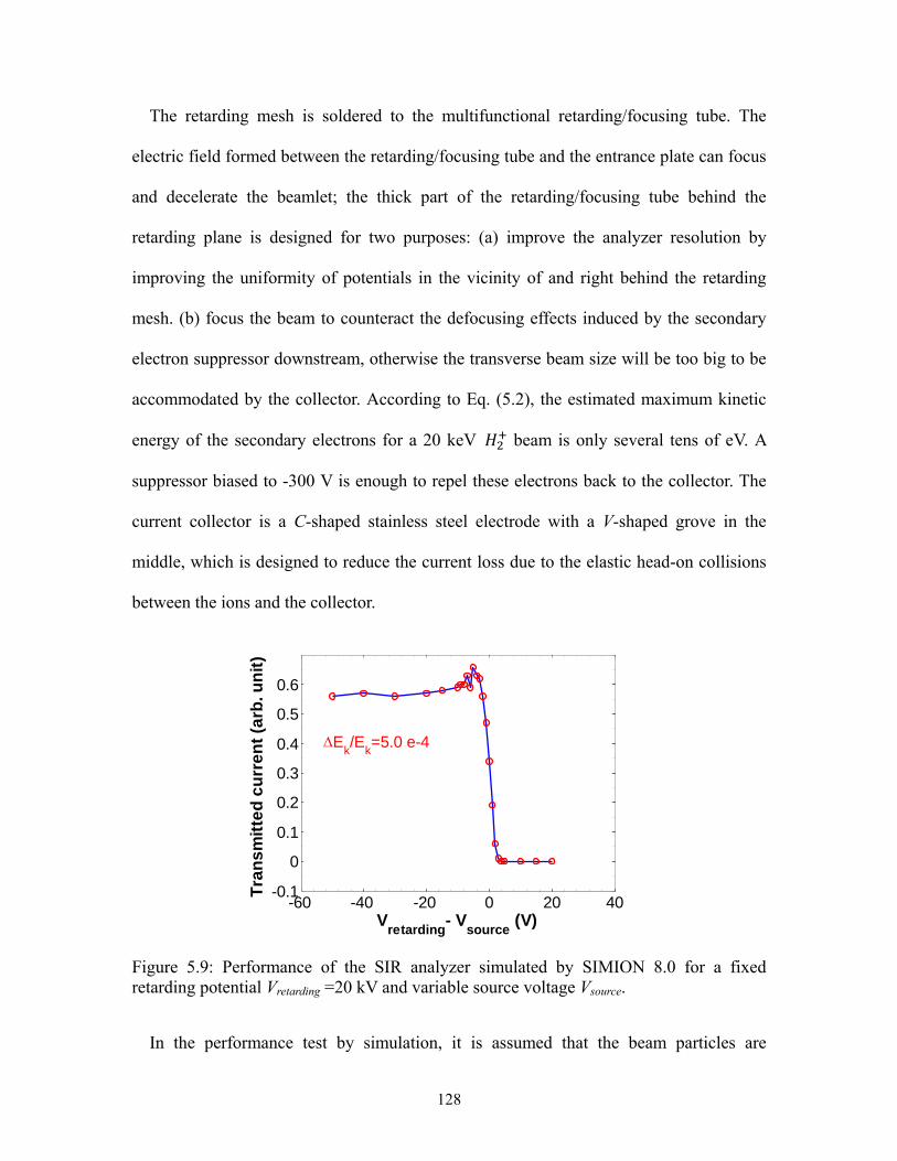
128
The retarding mesh is soldered to the multifunctional retarding/focusing tube. The
electric field formed between the retarding/focusing tube and the entrance plate can focus
and decelerate the beamlet; the thick part of the retarding/focusing tube behind the
retarding plane is designed for two purposes: (a) improve the analyzer resolution by
improving the uniformity of potentials in the vicinity of and right behind the retarding
mesh. (b) focus the beam to counteract the defocusing effects induced by the secondary
electron suppressor downstream, otherwise the transverse beam size will be too big to be
accommodated by the collector. According to Eq. (5.2), the estimated maximum kinetic
energy of the secondary electrons for a 20 keV beam is only several tens of eV. A
suppressor biased to -300 V is enough to repel these electrons back to the collector. The
current collector is a C-shaped stainless steel electrode with a V-shaped grove in the
middle, which is designed to reduce the current loss due to the elastic head-on collisions
between the ions and the collector.
Figure 5.9: Performance of the SIR analyzer simulated by SIMION 8.0 for a fixed retarding potential Vretarding =20 kV and variable source voltage Vsource.
In the performance test by simulation, it is assumed that the beam particles are
-60 -40 -20 0 20 40-0.1
0
0.1
0.2
0.3
0.4
0.5
0.6
Vretarding
- Vsource
(V)
Tra
ns
mit
ted
cu
rre
nt
(arb
. un
it)
Ek/E
k=5.0 e-4
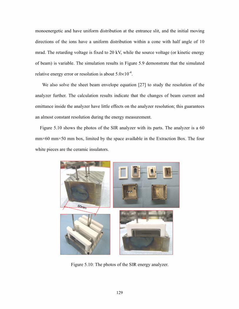
mono
direct
mrad
of be
relati
W
analy
emitt
an alm
Fig
mm×
white
oenergetic an
tions of the
d. The retardi
eam) is varia
ve energy er
We also solv
yzer further.
tance inside
most constan
gure 5.10 sh
60 mm×50
e pieces are t
nd have uni
ions have
ing voltage i
able. The sim
rror or resolu
e the sheet
The calcula
the analyzer
nt resolution
hows the pho
mm box, lim
the ceramic
Figure 5.1
form distrib
a uniform d
is fixed to 2
mulation resu
ution is abou
beam envel
ation results
r have little e
n during the e
otos of the S
mited by the
insulators.
10: The phot
129
bution at the
distribution w
0 kV, while
ults in Figur
ut 5.0μ10-4.
ope equation
s indicate th
effects on th
energy meas
SIR analyzer
e space avail
os of the SIR
entrance sli
within a con
the source v
re 5.9 demon
n [27] to stu
hat the chang
he analyzer r
surement.
r with its pa
lable in the E
R energy ana
it, and the in
ne with half
voltage (or k
nstrate that
udy the reso
ges of beam
resolution; th
arts. The ana
Extraction B
alyzer.
nitial movin
f angle of 1
kinetic energ
the simulate
olution of th
m current an
his guarantee
alyzer is a 6
Box. The fou
ng
10
gy
ed
he
nd
es
60
ur
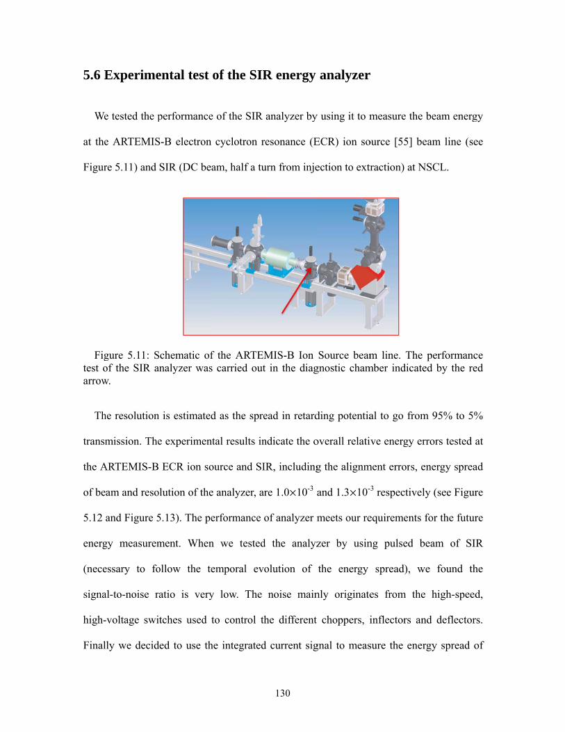
5.6 E
We
at the
Figur
Figtest oarrow
Th
transm
the A
of be
5.12
energ
(nece
signa
high-
Final
Experime
e tested the p
e ARTEMIS
re 5.11) and
gure 5.11: Sof the SIR aw.
he resolution
mission. The
ARTEMIS-B
am and reso
and Figure 5
gy measurem
essary to fo
al-to-noise r
-voltage swi
ly we decid
ental test
performance
S-B electron
SIR (DC be
Schematic ofanalyzer was
n is estimated
e experimen
ECR ion so
olution of the
5.13). The pe
ment. When
ollow the te
ratio is very
itches used
ded to use th
of the SIR
e of the SIR
cyclotron r
am, half a tu
f the ARTEMs carried out
d as the spre
ntal results in
ource and SI
e analyzer, ar
erformance o
n we tested
emporal ev
y low. The
to control th
he integrated
130
R energy
analyzer by
resonance (E
urn from inje
MIS-B Ion t in the diag
ead in retard
ndicate the o
IR, including
re 1.0μ10-3 a
of analyzer m
d the analyz
olution of
noise main
he different
d current sig
analyzer
y using it to m
ECR) ion so
ection to extr
Source beamgnostic cham
ding potentia
overall relati
g the alignm
and 1.3μ10-
meets our re
zer by usin
the energy
nly originate
choppers, i
gnal to meas
r
measure the
ource [55] be
traction) at N
m line. The mber indicate
al to go from
ive energy er
ment errors, e
-3 respectivel
equirements
ng pulsed b
spread), w
es from the
inflectors an
sure the ener
beam energ
eam line (se
NSCL.
performanced by the re
m 95% to 5%
rrors tested a
energy sprea
ly (see Figur
for the futur
beam of SI
we found th
e high-speed
nd deflector
rgy spread o
gy
ee
ce ed
%
at
ad
re
re
R
he
d,
rs.
of

131
SIR beam, which will be discussed in details in the next chapter.
Figure 5.12: Performance of the SIR energy analyzer tested at ARTEMIS-B ECR ion source.
Figure 5.13: Performance of the SIR energy analyzer tested at SIR by DC beam.
9900 9910 9920 9930 9940 9950
0
20
40
60
80
100
Vretarding
(V)
Cu
rre
nt
(A) E
k/E
k=1.0 e-3
10280 10290 10300 10310
0
50
100
150
200
Vretarding
(V)
Cu
rre
nt
(nA
) Ek/E
k=1.3 e-3
132
5.7 Conclusions
A compact, high resolution retarding field energy analyzer has been designed and
tested for SIR of NSCL at MSU to further study the beam instability. Experimental
results indicate the performance of the analyzer meets the requirements for our future
measurement and research work.

133
Chapter 6
NONLINEAR BEAM DYNAMICS OF SIR BEAM4
6.1 Introduction
When a high intensity uniform long bunch with a finite length is injected into the
SIR, the nonlinear space charge forces in the beam head and tail are strong and may
deform the beam shape. In addition, as the perturbation amplitude of the line charge
density increases due to microwave instability, the beam dynamics of the central part of
the beam also enters the nonlinear regime soon after injection. The bunch may break up
into many small clusters longitudinally only after several turns of coasting [12, 13]. This
chapter mainly discusses the nonlinear beam dynamics in these cases, including the study
on evolution of energy spread, vortex motion, and merging of cluster pairs by
experimental, simulation and analytical methods.
6.2 Measurement of the energy spread
Among the various beam parameters which govern the evolution of the bunched beam
profiles, the energy spread induced by the space charge field plays an important role in
both the linear and nonlinear regime of beam instability. It may help to suppress the
microwave instability in the linear beam dynamics; in addition, it is also one of the
important measures of the asymptotic bunch behavior in the nonlinear beam dynamics.
For this reason, an accurate knowledge of the energy spread distribution and evolution of 4 The contents regarding energy spread measurement and simulation is excerpted from Y. Li, L. Wang, F.
Lin, Nuclear Instruments and Methods in Physics Research A 763, 674 (2014).
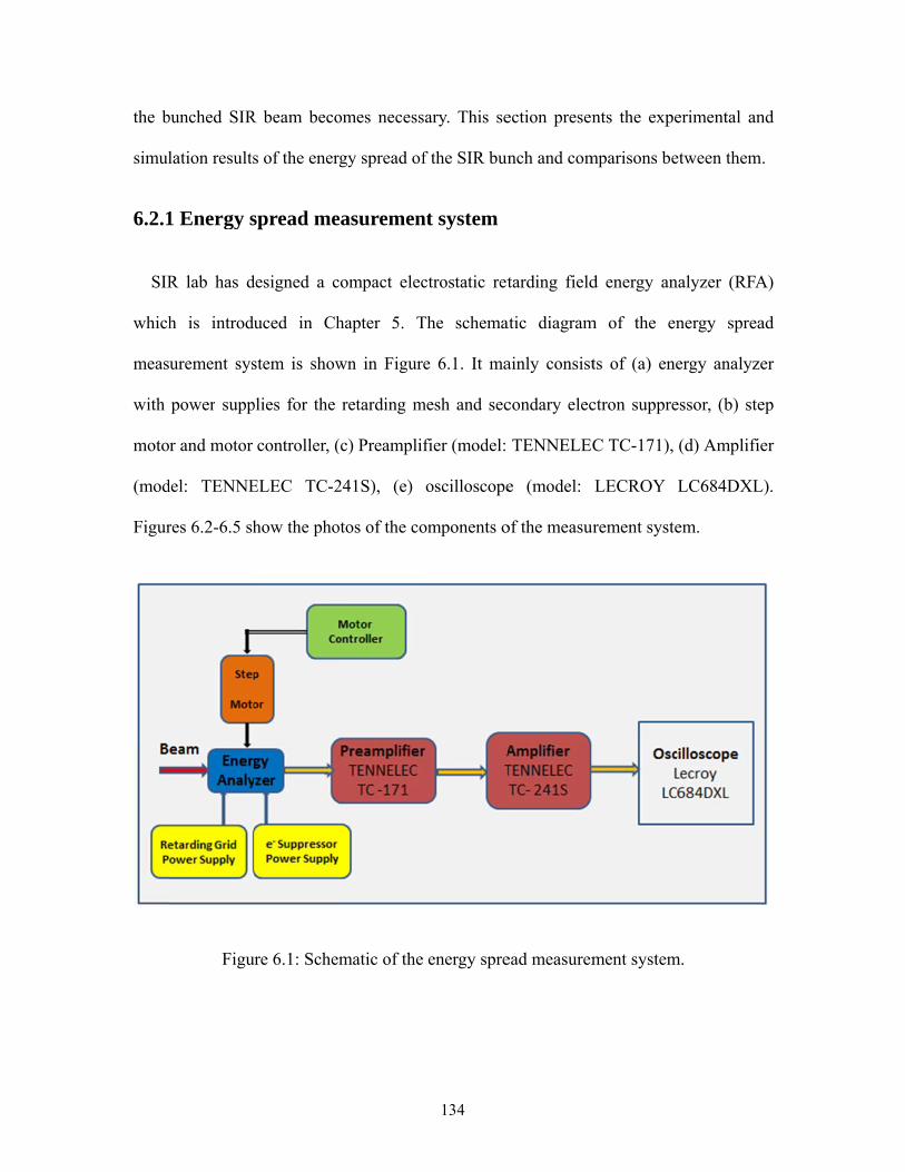
the b
simul
6.2.1
SIR
which
meas
with
moto
(mod
Figur
bunched SIR
lation results
1 Energy s
R lab has d
h is introdu
urement sys
power supp
r and motor
del: TENNE
res 6.2-6.5 sh
Figu
R beam beco
s of the ener
spread me
designed a c
uced in Ch
stem is show
plies for the
controller, (
ELEC TC-2
how the pho
ure 6.1: Sche
omes necess
rgy spread of
easuremen
compact elec
hapter 5. T
wn in Figur
retarding m
(c) Preamplif
241S), (e)
otos of the co
matic of the
134
sary. This se
f the SIR bun
nt system
ctrostatic ret
The schema
e 6.1. It ma
mesh and sec
fier (model:
oscilloscope
omponents o
energy spre
ection presen
nch and com
tarding field
atic diagram
ainly consist
condary elec
TENNELEC
e (model:
of the measur
ead measurem
nts the expe
mparisons be
d energy an
m of the en
ts of (a) ene
ctron suppre
C TC-171),
LECROY
urement syste
ment system
erimental an
etween them
nalyzer (RFA
nergy sprea
ergy analyze
essor, (b) ste
(d) Amplifie
LC684DXL
em.
m.
nd
.
A)
ad
er
ep
er
L).
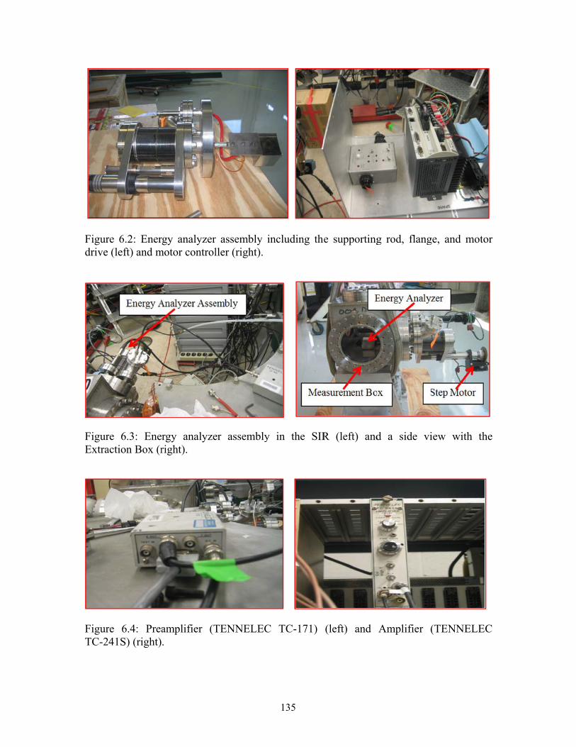
Figurdrive
FigurExtra
FigurTC-2
re 6.2: Ener (left) and m
re 6.3: Eneaction Box (r
re 6.4: Prea241S) (right)
rgy analyzermotor control
rgy analyzeright).
amplifier (T.
r assembly iller (right).
er assembly
TENNELEC
135
including th
y in the SIR
C TC-171)
he supporting
R (left) and
(left) and
g rod, flang
d a side vi
Amplifier (
ge, and moto
iew with th
(TENNELE
or
he
C
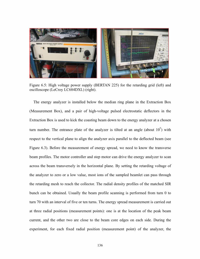
Figuroscill
Th
(Mea
Extra
turn
respe
Figur
beam
acros
the an
the re
bunch
turn 7
at thr
curre
exper
re 6.5: Highloscope (LeC
he energy an
asurement B
action Box is
number. Th
ect to the ver
re 6.3). Befo
m profiles. Th
ss the beam
nalyzer to z
etarding mes
h can be ob
70 with an in
ree radial po
nt, and the
riment, for
h voltage powCroy LC684
nalyzer is in
Box), and a
s used to kic
e entrance p
rtical plane t
ore the meas
he motor con
transversely
zero or a low
sh to reach t
btained. Usu
nterval of fiv
ositions (me
other two a
each fixed
wer supply DXL) (right
nstalled belo
pair of hig
ck the coastin
plate of the
to align the
surement of
ntroller and
y in the hori
w value, mos
the collector
ally the bea
ve or ten turn
easurement p
are close to
radial posi
136
(BERTAN 2t).
w the medi
gh-voltage p
ng beam dow
analyzer is
analyzer axi
f energy spre
step motor c
zontal plane
st ions of th
r. The radial
am profile sc
ns. The ener
points): one
the beam c
tion (measu
225) for the
an ring plan
pulsed electr
wn to the en
s tilted at an
is parallel to
ead, we nee
can drive the
e. By setting
he sampled b
l density pro
canning is p
rgy spread m
is at the lo
core edges o
urement poi
e retarding g
ne in the Ex
rostatic defl
nergy analyze
n angle (abo
o the deflect
d to know t
e energy ana
g the retardin
beamlet can
ofiles of the
performed fr
measurement
ocation of th
on each side
int) of the
grid (left) an
xtraction Bo
lectors in th
er at a chose
out 10o) wit
ted beam (se
the transvers
alyzer to sca
ng voltage o
pass throug
matched SI
rom turn 0 t
is carried ou
he peak beam
e. During th
analyzer, th
nd
ox
he
en
th
ee
se
an
of
gh
R
to
ut
m
he
he

137
retarding voltage is varied within a range in the vicinity of the nominal beam energy. The
current signals on the current collector of the analyzer are amplified by the Preamplifier
(TENNELEC TC-171) and Amplifier (TENNELEC TC-241S) consecutively. The
amplified signals are sent to the oscilloscope (LeCroy LC684DXL), where the
waveforms and strengths of the signals (in voltages) can be observed and read. After
offline data analysis, the energy spread information of the beam can be obtained.
6.2.2 Data analysis of the energy spread
A ion bunch with the length 600 mm, peak current 8.0 mA, kinetic energy 10.3
keV is used in the energy spread measurements. The measured emittance is about 30
mm mrad. From the measurement, the raw S-V curves at the three radial positions
(measurement points) and various turn numbers are obtained. Here S and V denote the
signal strength and the retarding voltage, respectively. The top graph of Figure 6.6 shows
an example of the measured raw S-V curve. For each fixed radial measurement point and
turn number, the data analysis for the energy spread measurement is performed by the
following procedure:
1. Subtract the residual noise signal from the raw S-V curve and normalize the adjusted
S-V curve to 1. This procedure yields a transmission rate curve (T-V curve) ranging
from 0 to 1.
2. Assuming the energy spread has a Gaussian distribution with deviation sE and mean
energy of <E>,
,2
1)(
2
2
2
)(
E
EE
E
eEP
(6.1)
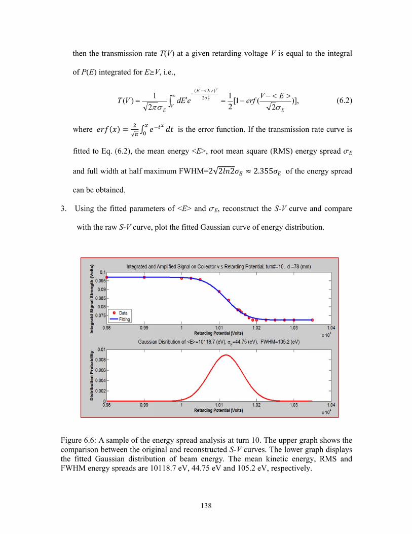
th
of
w
fi
an
ca
3. U
w
Figurcompthe fFWH
hen the trans
f P(E) integr
where (itted to Eq. (
nd full width
an be obtain
Using the fit
with the raw
re 6.6: A samparison betwfitted GaussiHM energy sp
smission rate
rated for E¥
2
1)(VT
) = √(6.2), the me
h at half max
ned.
tted paramet
w S-V curve,
mple of the eween the orig
ian distributpreads are 1
e T(V) at a g
V, i.e.,
1V
E
eEd
is the
ean energy <
ximum FWH
ters of <E>
plot the fitte
energy spreaginal and rection of beam0118.7 eV, 4
138
given retardi
2
12
2
2
)( EE
E
e error funct
<E>, root m
HM=2√2 2and sE, rec
ed Gaussian
ad analysis aconstructed Sm energy. T44.75 eV and
ing voltage
(1[2
1 Verf
tion. If the t
mean square 2 ≈ 2.355construct the
curve of ene
at turn 10. ThS-V curves. TThe mean kd 105.2 eV,
V is equal t
)],2 E
E
transmission
(RMS) ener5 of the e
e S-V curve
ergy distribu
he upper graThe lower g
kinetic energrespectively
to the integra
(6.2
n rate curve
rgy spread s
energy sprea
and compar
ution.
aph shows thgraph displaygy, RMS any.
al
2)
is
sE
ad
re
he ys nd

139
Note that the conventional method of energy spread analysis usually involves
differentiation of the S-V curve dS/dV and fitting it to a Gaussian function. While due to
the discreteness originating from the smaller number of data points in the vicinity of the
mean energy, the data points of dS/dV scatter around the Gaussian function with big
deviation. This makes the fitting work difficult and inaccurate. That is why an integral of
Gaussian function in Eq. (6.2) instead of the Gaussian function itself is chosen as the
curve fitting function in our energy spread analysis.
Figure 6.6 demonstrates a sample of the energy spread analysis results for the SIR
bunch measured at x= -6 mm (beam core edge) and turn 10. The mean kinetic energy,
RMS and FWHM energy spreads are 10118.7 eV, 44.75 eV and 105.2 eV, respectively.
6.2.3 Measurement results and comparisons with simulation
A 600 mm, 8.0 mA, 10.3 keV, 30 mm mrad (same parameters as those in
measurements) monoenergetic macroparticle bunch is also used in the simulation study
by the code CYCO. The bunch has a uniform initial distribution in both the longitudinal
line charge density and the 4D transverse phase space. In the analysis of simulation
results, the beam region is cut into several 1-mm-wide thin vertical slices which are
parallel to the design orbit, each thin slice has a fixed radial coordinate. The number of
macroparticles, mean kinetic energy and RMS energy spread in each slice are calculated
and compared with the experimental values.
Figure 6.7 shows the simulated and experimental radial slice beam densities. Figure 6.8
illustrates the simulated top views and slice RMS energy spread at turn 4 and turn 30,
respectively. Figure 6.9 displays the simulated slice RMS energy spread up to turn 8.
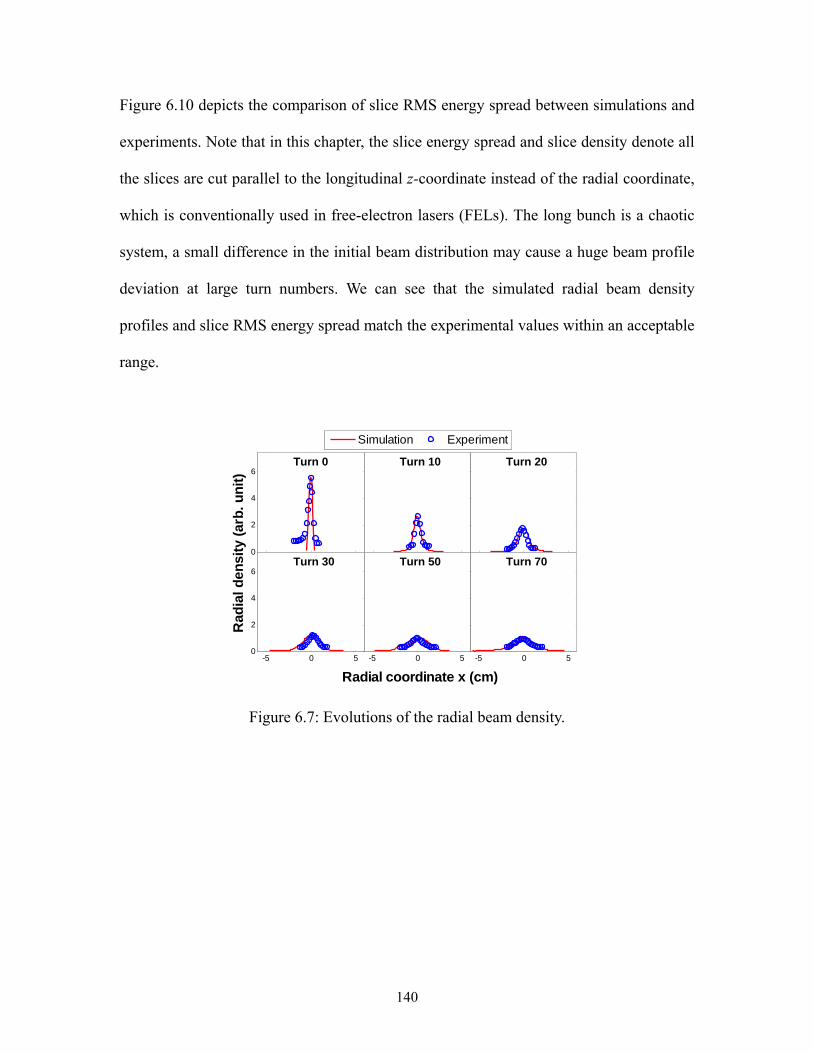
140
Figure 6.10 depicts the comparison of slice RMS energy spread between simulations and
experiments. Note that in this chapter, the slice energy spread and slice density denote all
the slices are cut parallel to the longitudinal z-coordinate instead of the radial coordinate,
which is conventionally used in free-electron lasers (FELs). The long bunch is a chaotic
system, a small difference in the initial beam distribution may cause a huge beam profile
deviation at large turn numbers. We can see that the simulated radial beam density
profiles and slice RMS energy spread match the experimental values within an acceptable
range.
Figure 6.7: Evolutions of the radial beam density.
Radial coordinate x (cm)
Rad
ial d
ensi
ty (
arb
. un
it)
0
2
4
6Turn 0 Turn 10 Turn 20
-5 0 50
2
4
6Turn 30
-5 0 5
Turn 50
-5 0 5
Turn 70
Simulation Experiment
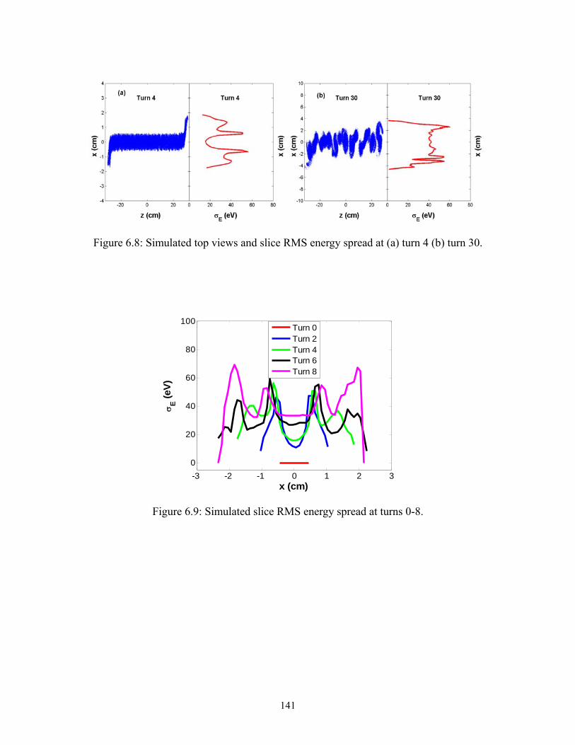
141
Figure 6.8: Simulated top views and slice RMS energy spread at (a) turn 4 (b) turn 30.
Figure 6.9: Simulated slice RMS energy spread at turns 0-8.
-3 -2 -1 0 1 2 3
0
20
40
60
80
100
x (cm)
E (
eV)
Turn 0Turn 2Turn 4Turn 6Turn 8
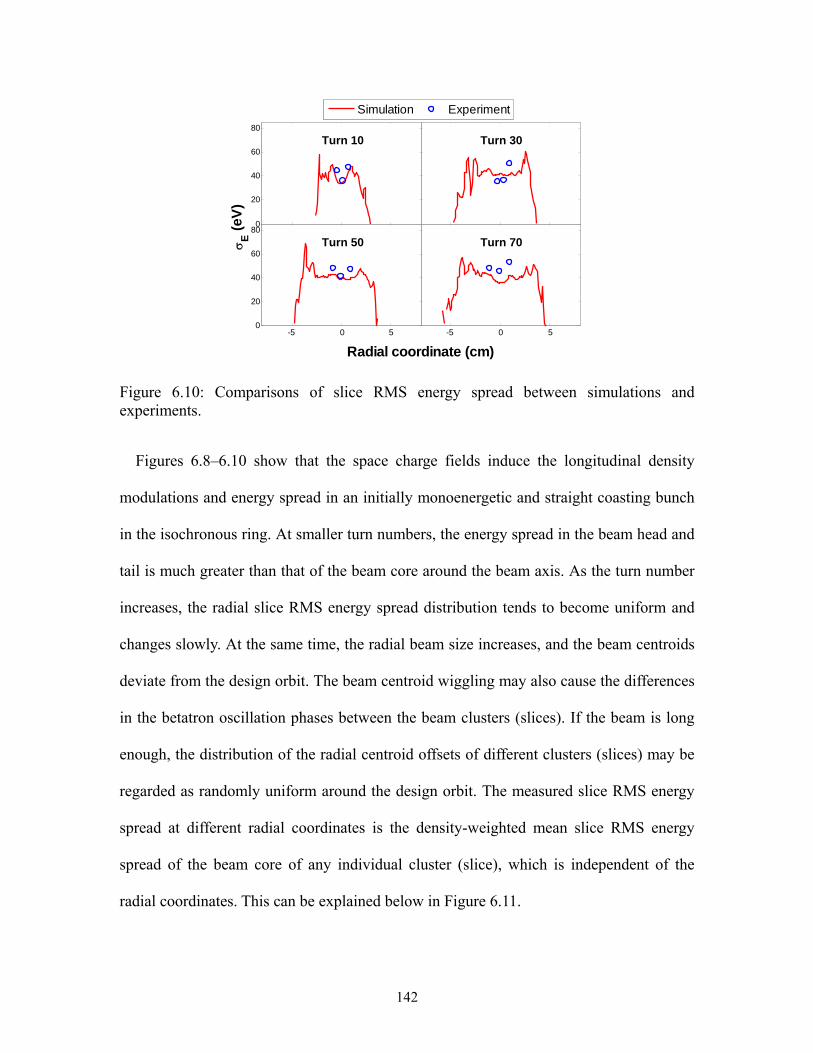
142
Figure 6.10: Comparisons of slice RMS energy spread between simulations and experiments.
Figures 6.8–6.10 show that the space charge fields induce the longitudinal density
modulations and energy spread in an initially monoenergetic and straight coasting bunch
in the isochronous ring. At smaller turn numbers, the energy spread in the beam head and
tail is much greater than that of the beam core around the beam axis. As the turn number
increases, the radial slice RMS energy spread distribution tends to become uniform and
changes slowly. At the same time, the radial beam size increases, and the beam centroids
deviate from the design orbit. The beam centroid wiggling may also cause the differences
in the betatron oscillation phases between the beam clusters (slices). If the beam is long
enough, the distribution of the radial centroid offsets of different clusters (slices) may be
regarded as randomly uniform around the design orbit. The measured slice RMS energy
spread at different radial coordinates is the density-weighted mean slice RMS energy
spread of the beam core of any individual cluster (slice), which is independent of the
radial coordinates. This can be explained below in Figure 6.11.
Radial coordinate (cm)
E (
eV)
0
20
40
60
80
Turn 10 Turn 30
-5 0 50
20
40
60
80
Turn 50
-5 0 5
Turn 70
Simulation Experiment
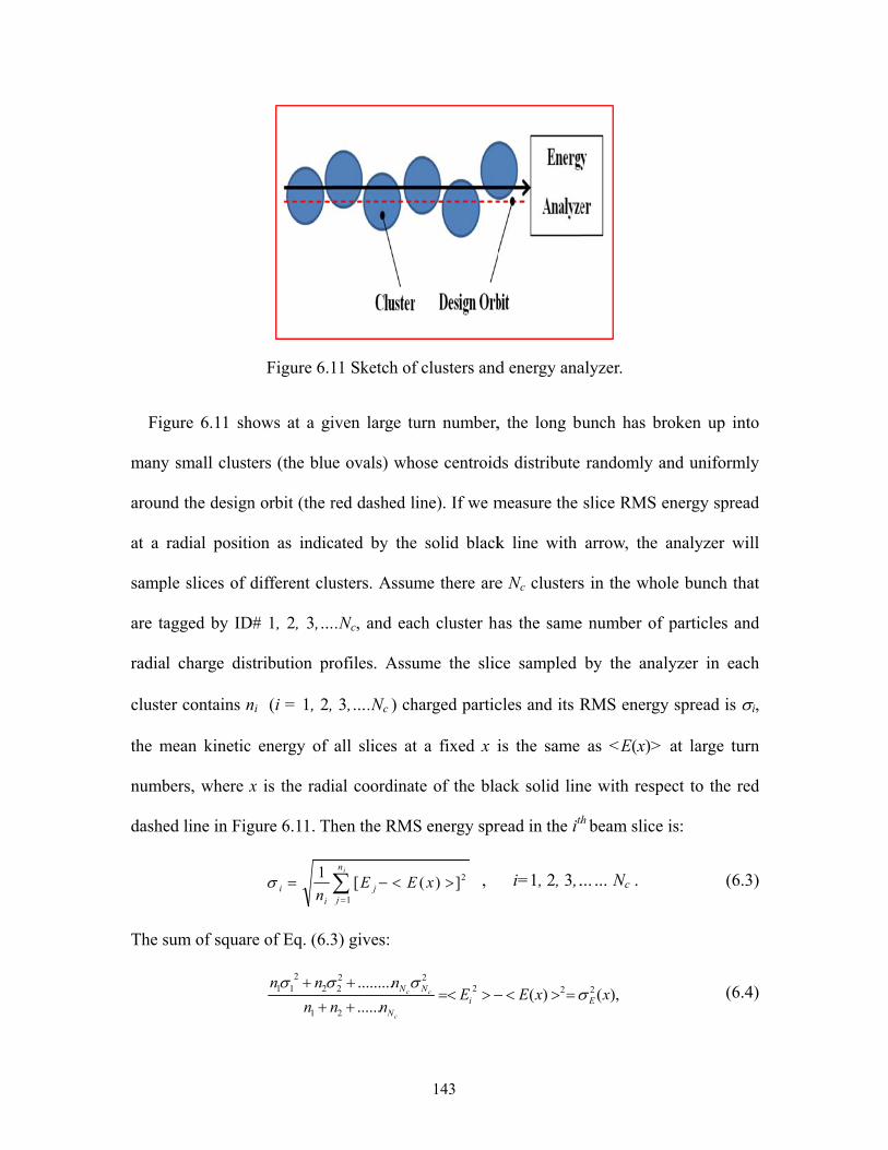
Fig
many
aroun
at a
samp
are ta
radial
cluste
the m
numb
dashe
The s
gure 6.11 sh
y small clust
nd the design
radial positi
ple slices of
agged by ID
l charge dis
er contains n
mean kinetic
bers, where x
ed line in Fig
sum of squar
Figure 6.1
hows at a gi
ters (the blu
n orbit (the r
ion as indic
different clu
D# 1, 2, 3,…
stribution pr
ni (i = 1, 2,
c energy of
x is the radi
gure 6.11. Th
ii n
1
re of Eq. (6.3
1
22
11
nn
nn
11 Sketch of
iven large tu
e ovals) wh
red dashed l
cated by the
usters. Assum
….Nc, and eac
rofiles. Assu
3,….Nc ) ch
all slices at
ial coordinat
hen the RMS
in
jj EE
1
[
3) gives:
......
.........
2
22
nn
n
N
N
c
c
143
f clusters and
urn number,
ose centroid
ine). If we m
e solid black
me there are
ch cluster ha
ume the slic
harged partic
t a fixed x i
te of the bla
S energy spr
xE 2])( ,
22
EiNc
d energy ana
, the long b
ds distribute
measure the
k line with
e Nc clusters
as the same
ce sampled
cles and its R
is the same
ack solid lin
read in the ith
i=1, 2, 3,…
)( 2xE
alyzer.
unch has br
randomly a
slice RMS e
arrow, the
s in the who
e number of
by the anal
RMS energy
as <E(x)>
ne with respe
h beam slice
…… Nc .
),(2 xE
roken up int
and uniforml
energy sprea
analyzer wi
ole bunch tha
particles an
lyzer in eac
y spread is
at large tur
ect to the re
is:
(6.3
(6.4
to
ly
ad
ill
at
nd
ch
i,
rn
ed
3)
4)
144
.]
......
.........[)( 2
1
21
2222
211
c
cc
N
NNE nnn
nnnx
(6.5)
If the number of clusters is large enough and the radial centroid offsets of all the
clusters are randomly and uniformly distributed around the design orbit, the RHS of Eq.
(6.5) is the density-weighted mean RMS energy spread of the sampled beam slices of
different cluster cores at a fixed radial coordinate x. The sE(x) of Eq. (6.5) is actually
equal to the density-weighed mean slice RMS energy spread of any given single cluster
core and is independent of the coordinate x. In real measurements, the above ideal
preconditions are not satisfied completely; hence, there are always small energy spread
fluctuations among different radial measurement points.
The equilibrium value of the kinetic energy deviation Eeq(x)=Eeq(x)-Ek0 and the radial
coordinate x of an off-momentum particle satisfy the relation
,2
)( 0 xR
ExE k
eq (6.6)
where Eeq (x) is the equilibrium kinetic energy and is equal to <E(x)> of the beam slices
centered at x at large turn numbers. For simplicity, it is assumed that the radial beam
density distribution is uniform. Then the RMS energy spread of the equilibrium particles
measured by the SIR energy analyzer with an entrance slit of width = 1 mm centered at
x can be estimated as:
.7.53
]')]'(2
[1
[ 02
120
2
2
eVR
Edxxx
R
E kk
x
x
Eeq
(6.7)
This value is proportional to the slit width and is independent of x. In addition, it is
much less than the asymptotic energy spread which is about 50 eV at large turn numbers.
This indicates that the number of particles at equilibrium energy only accounts for a small
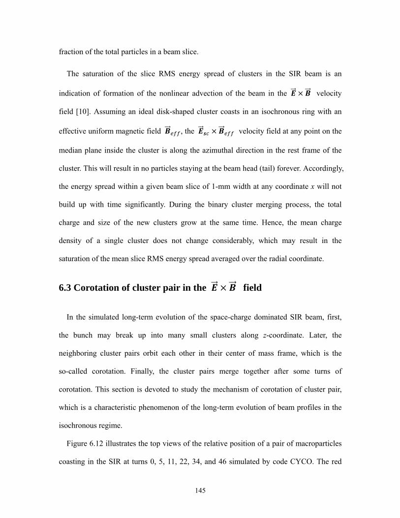
145
fraction of the total particles in a beam slice.
The saturation of the slice RMS energy spread of clusters in the SIR beam is an
indication of formation of the nonlinear advection of the beam in the × velocity
field [10]. Assuming an ideal disk-shaped cluster coasts in an isochronous ring with an
effective uniform magnetic field , the × velocity field at any point on the
median plane inside the cluster is along the azimuthal direction in the rest frame of the
cluster. This will result in no particles staying at the beam head (tail) forever. Accordingly,
the energy spread within a given beam slice of 1-mm width at any coordinate x will not
build up with time significantly. During the binary cluster merging process, the total
charge and size of the new clusters grow at the same time. Hence, the mean charge
density of a single cluster does not change considerably, which may result in the
saturation of the mean slice RMS energy spread averaged over the radial coordinate.
6.3 Corotation of cluster pair in the × field
In the simulated long-term evolution of the space-charge dominated SIR beam, first,
the bunch may break up into many small clusters along z-coordinate. Later, the
neighboring cluster pairs orbit each other in their center of mass frame, which is the
so-called corotation. Finally, the cluster pairs merge together after some turns of
corotation. This section is devoted to study the mechanism of corotation of cluster pair,
which is a characteristic phenomenon of the long-term evolution of beam profiles in the
isochronous regime.
Figure 6.12 illustrates the top views of the relative position of a pair of macroparticles
coasting in the SIR at turns 0, 5, 11, 22, 34, and 46 simulated by code CYCO. The red
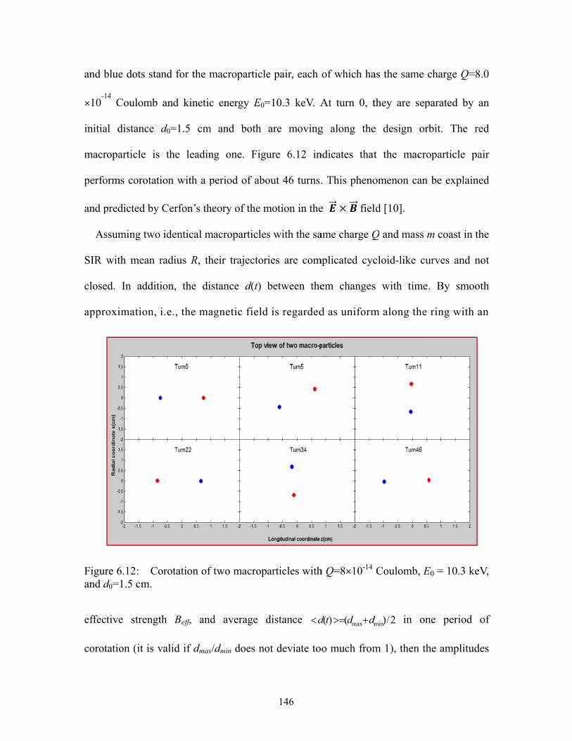
and b
ä10-1
initia
macro
perfo
and p
As
SIR w
close
appro
Figurand d
effect
corot
blue dots sta
4 Coulomb
al distance
oparticle is
orms corotati
predicted by
ssuming two
with mean r
d. In additi
oximation, i
re 6.12: Cod0=1.5 cm.
tive strengt
tation (it is v
and for the m
and kinetic
d0=1.5 cm
the leadin
ion with a p
Cerfon’s the
identical ma
radius R, th
ion, the dis
i.e., the mag
orotation of t
th Beff, and
valid if dmax/
macroparticle
energy E0=
and both
g one. Figu
period of abo
eory of the m
acroparticles
eir trajector
stance d(t) b
gnetic field
two macropa
d average d
/dmin does no
146
e pair, each
=10.3 keV. A
are moving
ure 6.12 in
out 46 turns.
motion in the
s with the sa
ies are com
between the
d is regarded
articles with
distance d
ot deviate to
of which ha
At turn 0, t
g along the
ndicates that
. This pheno
e × fiel
ame charge Q
mplicated cyc
em changes
d as uniform
h Q=8ä10-14
()( mmax ddtd
oo much from
as the same c
they are sep
e design or
t the macro
omenon can
ld [10].
Q and mass m
cloid-like cu
s with time
m along the
Coulomb, E
2/)mind in on
m 1), then th
charge Q=8.
parated by a
rbit. The re
oparticle pa
be explaine
m coast in th
urves and no
. By smoot
ring with a
E0 = 10.3 keV
ne period o
he amplitude
.0
an
ed
air
ed
he
ot
th
an
V,
of
es

147
of and space charge field can be estimated as
,0
eR
mvBeff ,
)(4 20
td
QEsc
(6.8)
where e, and v0 stand for the charge and velocity of each macroparticle, respectively.
Since and are perpendicular to each other, each macroparticle has a drift
velocity
.)(4
||||2
02
tdB
Q
B
E
B
BEVV
effeff
sc
eff
effscdriftdrift
(6.9)
The mean corotation frequency is
.2
2
30
.
dB
Qd
V
eff
driftcorot
(6.10)
The left graph of Figure 6.13 shows the simulated distance d(t) between the
macroparticle pair in the first period of corotation. The right graph displays the simulated
corotation angle of a line connecting the macroparticle pair with respect to +z-coordinate;
the corotation frequency is fitted and compares with the theoretical estimation predicted
by Eq. (6.10). We can see the simulation and theory match well.
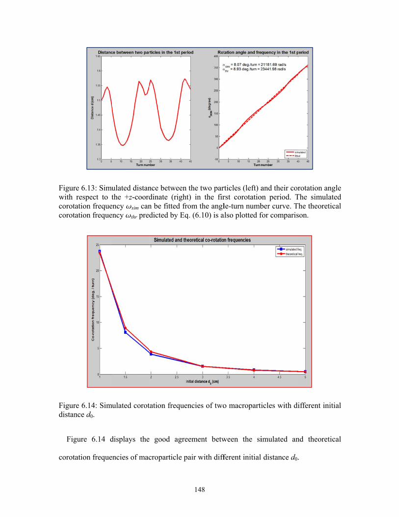
Figurwith corotcorot
Figurdistan
Fig
corot
re 6.13: Simurespect to t
tation frequetation freque
re 6.14: Simnce d0.
gure 6.14 d
tation freque
ulated distanthe +z-coord
ency wsim canency wthr pre
mulated corot
displays the
encies of mac
nce between dinate (rightn be fitted frdicted by Eq
tation freque
e good agre
croparticle p
148
the two part) in the firrom the anglq. (6.10) is a
encies of two
eement betw
pair with diff
rticles (left) arst corotatiole-turn numb
also plotted f
o macroparti
ween the si
ferent initial
and their coron period. Tber curve. Thfor comparis
icles with di
imulated an
distance d0.
rotation anglThe simulatehe theoretica
son.
ifferent initia
nd theoretica
.
le ed al
al
al
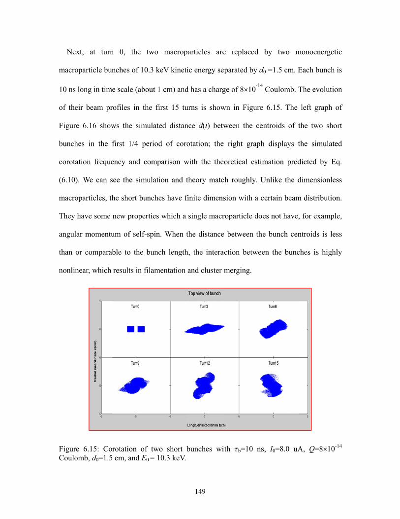
Ne
macro
10 ns
of th
Figur
bunch
corot
(6.10
macro
They
angul
than
nonli
FigurCoulo
ext, at turn
oparticle bun
s long in tim
eir beam pr
re 6.16 show
hes in the f
tation freque
0). We can s
oparticles, th
y have some
lar momentu
or comparab
near, which
re 6.15: Coomb, d0=1.5
n 0, the tw
nches of 10.
e scale (abou
rofiles in the
ws the simu
first 1/4 per
ency and co
see the simu
he short bun
new propert
um of self-s
ble to the b
results in fil
rotation of cm, and E0
wo macrop
3 keV kineti
ut 1 cm) and
e first 15 tu
ulated distan
riod of coro
omparison w
ulation and t
nches have f
ties which a
pin. When t
bunch length
lamentation
two short b= 10.3 keV.
149
particles are
ic energy sep
d has a charg
urns is show
nce d(t) betw
otation; the
with the theo
theory match
finite dimens
single macr
the distance
h, the interac
and cluster m
bunches wit
e replaced
parated by d
ge of 8ä10-14
wn in Figure
ween the ce
right graph
oretical esti
h roughly. U
sion with a c
roparticle do
between th
ction betwee
merging.
th tb=10 ns
by two m
d0 =1.5 cm. E
4 Coulomb. T
e 6.15. The
entroids of t
h displays t
mation pred
Unlike the d
certain beam
oes not have,
he bunch cen
en the bunc
s, I0=8.0 uA
monoenergeti
Each bunch
The evolutio
left graph o
the two sho
the simulate
dicted by Eq
dimensionles
m distribution
, for exampl
ntroids is les
ches is highl
A, Q=8ä10-
ic
is
on
of
ort
ed
q.
ss
n.
e,
ss
ly
14
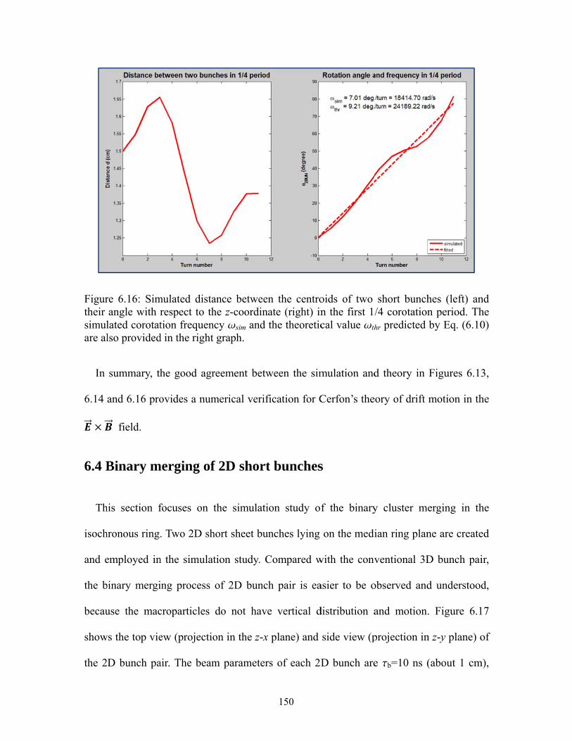
Figurtheir simulare al
In
6.14 ×6.4 B
Th
isoch
and e
the b
becau
show
the 2
re 6.16: Simangle with rlated corotatlso provided
summary, th
and 6.16 pro
field.
Binary m
his section f
hronous ring.
employed in
binary mergi
use the mac
ws the top vie
D bunch pa
mulated distarespect to thtion frequen
d in the right
he good agr
ovides a num
merging of
focuses on t
. Two 2D sh
n the simulat
ing process
croparticles
ew (projectio
air. The beam
ance betweehe z-coordincy wsim and graph.
reement betw
merical verif
f 2D short
the simulati
hort sheet bu
tion study. C
of 2D bunc
do not hav
on in the z-x
m parameter
150
en the centronate (right) in
the theoretic
ween the sim
fication for C
t bunches
ion study of
unches lying
Compared w
ch pair is ea
e vertical d
x plane) and
rs of each 2D
oids of two n the first 1/cal value wth
mulation and
Cerfon’s the
s
f the binary
on the medi
with the conv
asier to be o
distribution a
side view (p
D bunch are
short bunch/4 corotationhr predicted
d theory in
eory of drift
y cluster me
ian ring plan
ventional 3D
observed and
and motion.
projection in
e tb=10 ns (
hes (left) ann period. Thby Eq. (6.10
Figures 6.13
motion in th
erging in th
ne are create
D bunch pai
d understood
. Figure 6.1
n z-y plane) o
(about 1 cm
nd he 0)
3,
he
he
ed
ir,
d,
17
of
m),
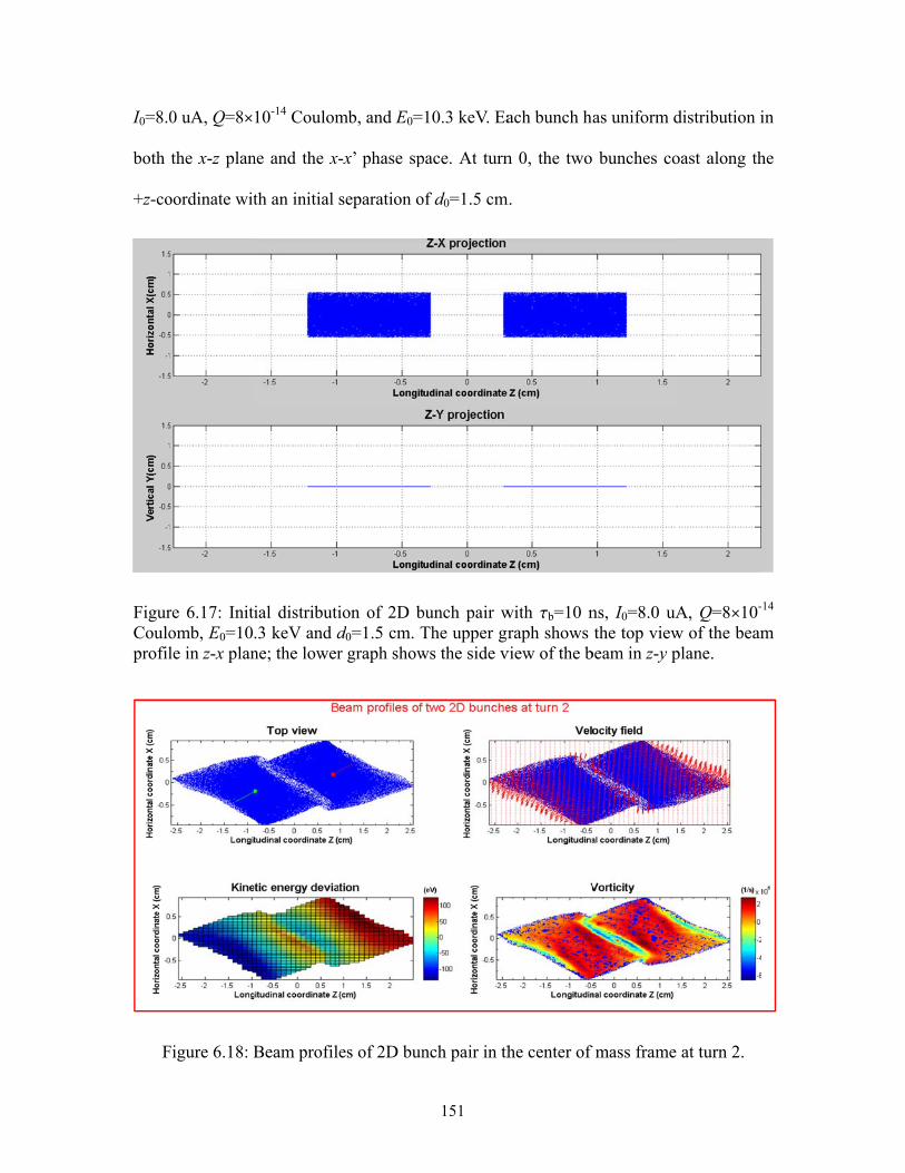
I0=8.0
both
+z-co
FigurCouloprofil
F
0 uA, Q=8ä
the x-z plan
oordinate wit
re 6.17: Initomb, E0=10le in z-x plan
Figure 6.18: B
10-14 Coulom
ne and the x
th an initial
ial distributi.3 keV and dne; the lower
Beam profil
mb, and E0=
-x’ phase sp
separation o
ion of 2D bd0=1.5 cm. Tr graph show
es of 2D bun
151
10.3 keV. Ea
pace. At turn
of d0=1.5 cm
bunch pair wThe upper grws the side v
nch pair in th
ach bunch ha
n 0, the two
m.
with tb=10 nraph shows
view of the b
he center of
as uniform d
bunches co
ns, I0=8.0 uAthe top view
beam in z-y p
f mass frame
distribution i
oast along th
A, Q=8ä10-
w of the beamplane.
at turn 2.
in
he
14 m
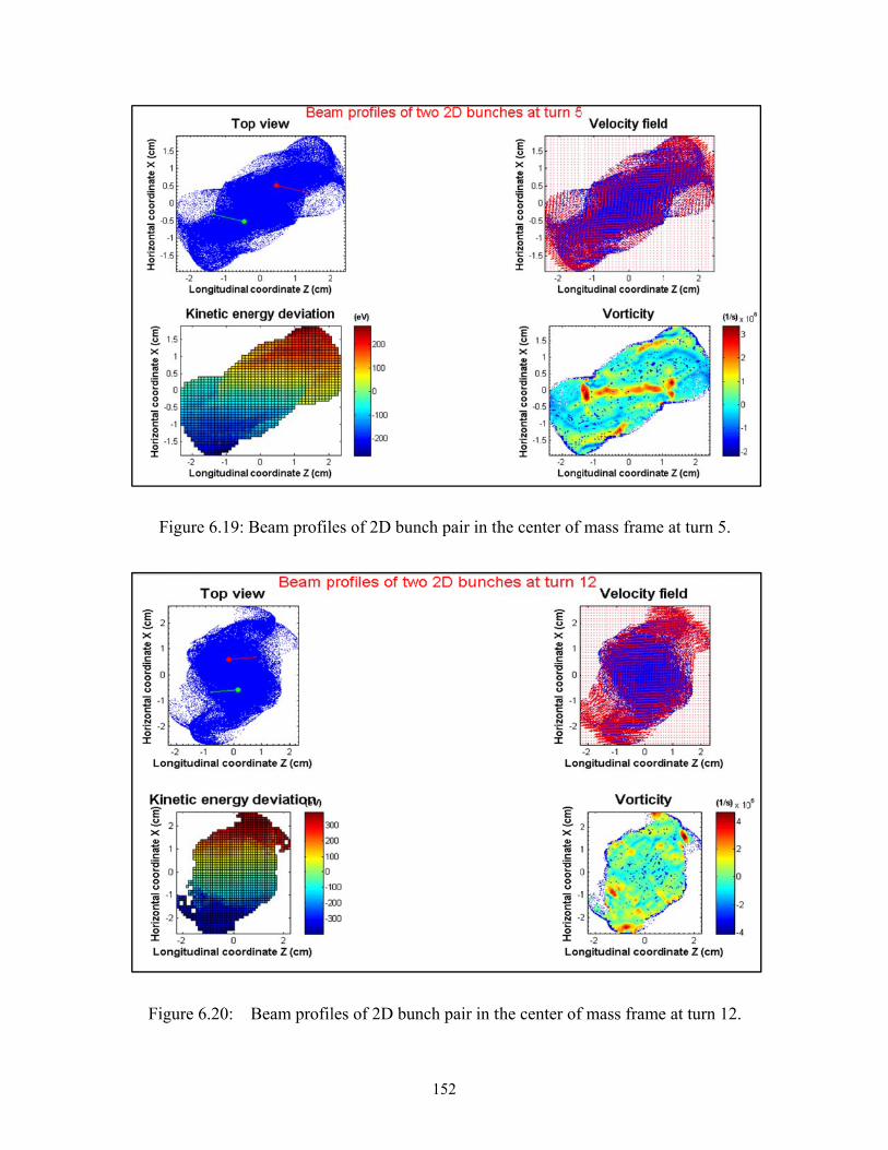
F
Fig
Figure 6.19: B
gure 6.20:
Beam profil
Beam profil
es of 2D bun
les of 2D bun
152
nch pair in th
nch pair in t
he center of
the center of
f mass frame
f mass frame
at turn 5.
e at turn 12.
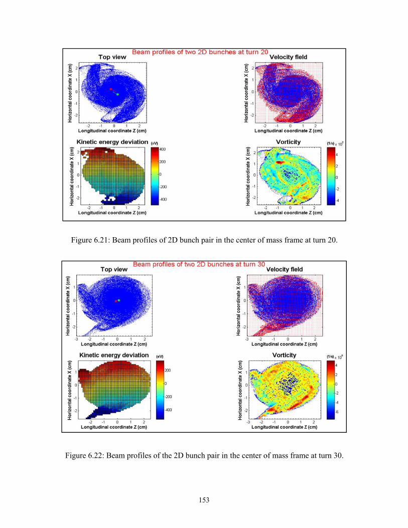
Fi
Figu
igure 6.21: B
ure 6.22: Be
Beam profile
eam profiles
es of 2D bun
of the 2D bu
153
nch pair in th
unch pair in
he center of m
the center o
mass frame
of mass fram
at turn 20.
me at turn 30.

154
Figures 6.18-6.22 illustrate the evolution of the beam density, energy deviation
distribution, velocity field and vorticity of the two short 2D bunches at turns 2, 5, 12, 20
and 30. Each figure consists of four graphs: the upper left graph shows the top view of
the beam density distribution on the median ring plane, the red and blue dots with arrows
stand for the centroids of the bunches and their velocity vectors in the center of mass
frame; the upper right graph displays the velocity field in the center of mass frame; the
lower left graph demonstrates the distribution of energy deviation of the 2D bunches; the
lower right graph depicts the distribution of vorticity, which is defined as the curl of the
speed vector u
in the center of mass frame:
.),( utx
(6.13)
During the merging process, the two bunches are highly deformed and two filament
tails appear. The two beam cores approach, overlap and collide; at first, the two centroids
corotate in the counter clockwise direction just like two macroparticles. But the repulsive
Coulomb force between two bunches causes dynamical friction, which decreases the
kinetic energy of the two centroids. The relative motion between the two centroids is
suppressed. This is completely different from the two macroparticle model in which each
macroparticle is dimensionless; the dynamic friction between the two macroparticle is
negligible, and the corotation motion can last forever. We can also use the theory of drift
motion in × field to explain the merging process. When the two bunch cores
overlap partly, the space charge force on the overlapping parts is cancelled significantly.
In consequence, the drift motion in the × field will be suppressed considerably. The
overlapping parts of the two bunches will become the cradle of a new beam core.
155
6.5 Conclusions
The measured slice RMS energy spread and radial density profiles of a long coasting
bunch agree with the simulation results. At large turn numbers, the randomly distributed
cluster centroid offsets tend to make the radial energy spread distribution of the whole
bunch uniform. The measured energy spread is the density-weighted mean slice RMS
energy spread of any single cluster core. Its saturation behavior indicates the formation of
the nonlinear advection of the particles due to the × velocity field in each cluster.
The simulation study of corotation of cluster pair by macroparticle pair model and
short bunch pair model verifies the theory of drift motion in the × field. The
corotation and merging of cluster pair in the long-term evolution of beam profiles is a
natural consequence of the drift motion of clusters in the × field.

156
Chapter 7
CONCLUSIONS AND FUTURE WORKS
7.1 Conclusions
This dissertation focuses on the mechanism and evolution of microwave instability of
coasting beams with space charge in the isochronous regime.
Several theoretical LSC impedance models with different cross-sections of the beam
and chamber are studied. The derived LSC impedances are in good agreement with the
numerical simulations. They can be used in instability analysis induced by the LSC field
at any perturbation wavelength l. In particular, for l<5cm, the LSC impedance of SIR
beam can be approximated by that of a round beam in free space.
For a beam with finite energy spread, due to the non-zero transfer matrix element
R56(s), the particles with the same radial coordinates (x, x£) in the radial phase space but
with deferent energies may have different path length difference Dz; In addition, due to
the betatron oscillation and radial-longitudinal coupling effect, the particles with the same
energy deviation but with different radial coordinates (x, x£) in the radial phase space also
have different path length difference Dz via the transfer matrix elements R51(s) and R52(s).
These path length differences are the important source of Landau damping for coasting
beam with finite emittance and energy spread in the isochronous ring. The path length
deviation contributed from the betatron motion in the isochronous rings is also an
important effect that should be considered to realize the coherent terahertz synchrotron
radiation (CSR) [56], in which case the length of an extremely short electron bunch needs
157
to be preserved precisely. A 2D dispersion relation taking into account the Landau
damping effects originating from the energy spread and emittance is derived in Chapter 4.
Compared with the conventional 1D growth rate formula, the 2D dispersion relation
provides a more accurate approach to predict the instability growth rates, especially in the
short wavelength limits.
A compact retarding field energy analyzer (RFA) with large entrance slit was designed,
tested and employed in the energy spread measurement. The performance of the RFA
meets our requirement for the experimental study of microwave instability.
The energy spread measurement results of a coasting SIR beam match the simulation
results in the long term evolution of microwave instability. The measured and simulated
saturation of the radial distribution of energy spread at large turn number is caused by the
formation of vortex motion in the bunches’ rest frames. The study using the
two-macroparticle model and the two-bunch model also validate the theory of vortex
motion in the × field.
7.2 Future works
Some new research study may be performed in the future, such as:
In Chapter 4, there exist bigger discrepancies between the theoretical and
simulated instability growth rates for l<1 cm. Further research study is needed to
explain the reason for the discrepancies.
In recent years, a 3D PIC object-oriented parallel simulation code OPAL-CYCL
has been successfully developed by PSI [17]. Being a parallel code, it can
simulate beam dynamics in high intensity cyclotrons including neighboring

158
bunch effects. Some interesting results have been obtained by the PSI researchers
[18, 57]. In comparison, CYCO is incapable of parallel computation at present. If
possible, CYCO can be modified to be compatible with parallel computation in
the future. This may greatly enhance its efficiency and functionality.
After years of successful operation with fruitful results, the Small Isochronous
Ring (SIR) was dismantled in 2010. If possible, it may be reassembled and
upgraded in the future (e.g., introduction of RF cavity, flat-top cavity, and new
energy spread measurement system, etc.). After upgrade, more research studies
regarding the space charger effects in isochronous regime can be carried out.

159
APPENDICES
160
APPENDIX A
FORMALISM OF THE STANDARD TRANSFER MATRIX
FOR SIR
This note presents the linear beam optics of SIR lattice (hard-edge model) using the
standard transfer matrix formalism.
A.1 Brief review of the standard transfer matrix
The coordinates of a particle in the 6D phase space can be described by a 6-element
vector (x(s), x£(s), y(s), y£(s), z(s), d(s))T [58-60], where x, y and z are the radial
(horizontal), vertical and longitudinal coordinates with respect to a hypothetical
on-momentum particle traveling along the design orbit; x£(s)=dx/ds and y£(s)=dy/ds are
the radial (horizontal) and vertical slopes of velocity; d=Dp/p is the fractional momentum
deviation compared with the on-momentum particle, the superscript ‘T’ stands for the
transpose of vector or matrix. If there is no electric field and x-y coupling, the standard
transfer matrix M(s) mapping the initial coordinates of a particle (x(0), x£(0), y(0), y£(0),
z(0), d(0))T in the 6D phase space at s=0 to the current ones (x(s), x£(s), y(s), y£(s), z(s),
d(s))T at s is [58-60]
161
.
100000
100
0000
0000
000
000
)0()0()0()0()0()0(
)0()0()0()0()0()0(
)0()0()0()0()0()0(
)0()0()0()0()0()0(
)0()0()0()0()0()0(
)0()0()0()0()0()0(
)(
565251
4443
3433
262221
161211
MMM
MM
MM
MMM
MMM
zyyxx
z
z
z
y
z
y
z
x
z
x
z
y
z
y
y
y
y
y
x
y
x
y
y
z
y
y
y
y
y
x
y
x
y
x
z
x
y
x
y
x
x
x
x
x
x
z
x
y
x
y
x
x
x
x
x
sM
(A.1)
The matrix M(s) satisfies the symplectic condition MTSM=S, where S is a 6μ6
antisymmetric matrix
,
010000
100000
000100
001000
000001
000010
S (A.2)
The determinant of matrix M(s) is unity, e.g., det(M)=1, which is required by
Liouville’s theorem. Some elements of the standard matrix M(s) satisfy the following
relations [8, 60, 61]:
,)(
)()(
)(
)()()(
0
12110
111216 sd
s
sMsMsd
s
sMsMsM
ss
(A.3)
,)(
)()(
)(
)()()(
0
12210
112226 sd
s
sMsMsd
s
sMsMsM
ss
(A.4)
,1126211651 MMMMM (A.5)
,1226221652 MMMMM (A.6)
where r(s) is the local radius of curvature of the orbit.
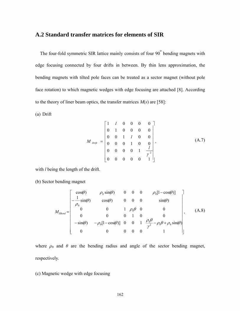
162
A.2 Standard transfer matrices for elements of SIR
The four-fold symmetric SIR lattice mainly consists of four 90o bending magnets with
edge focusing connected by four drifts in between. By thin lens approximation, the
bending magnets with tilted pole faces can be treated as a sector magnet (without pole
face rotation) to which magnetic wedges with edge focusing are attached [8]. According
to the theory of liner beam optics, the transfer matrices M(s) are [58]:
(a) Drift
,
100000
10000
001000
00100
000010
00001
2
l
l
l
M Drift (A.7)
with l being the length of the drift.
(b) Sector bending magnet
,
100000
)sin(100)]cos(1[)sin(
001000
00100
)sin(000)cos()sin(1
)]cos(1[000)sin()cos(
0020
0
0
0
00
SBendM (A.8)
where r0 and q are the bending radius and angle of the sector bending magnet,
respectively.
(c) Magnetic wedge with edge focusing
163
,
100000
010000
001)tan(
00
000100
00001)tan(
000001
0
0
EdgeM (A.9)
with j being the pole face rotation angle.
A.3 Optic functions of SIR (hard-edge model)
Let us consider the general condition of isochronism of a relativistic particle traveling
along an N-fold symmetric isochronous ring with edge focusing (See Figure A.1). The
transfer matrix of 1/2N period (half-cell) of the ring lattice is
.2
1 DfiftEdgeSBendCell
MMMM (A.10)
Substituting Eqs. (A.7), (A.8) and (A.9) into Eq. (A.10) with q=p/N yields
,
100000
100
0000
0000
000
000
565251
4443
3433
262221
161211
2
1
MMM
MM
MM
MMM
MMM
Mcell
(A.11)
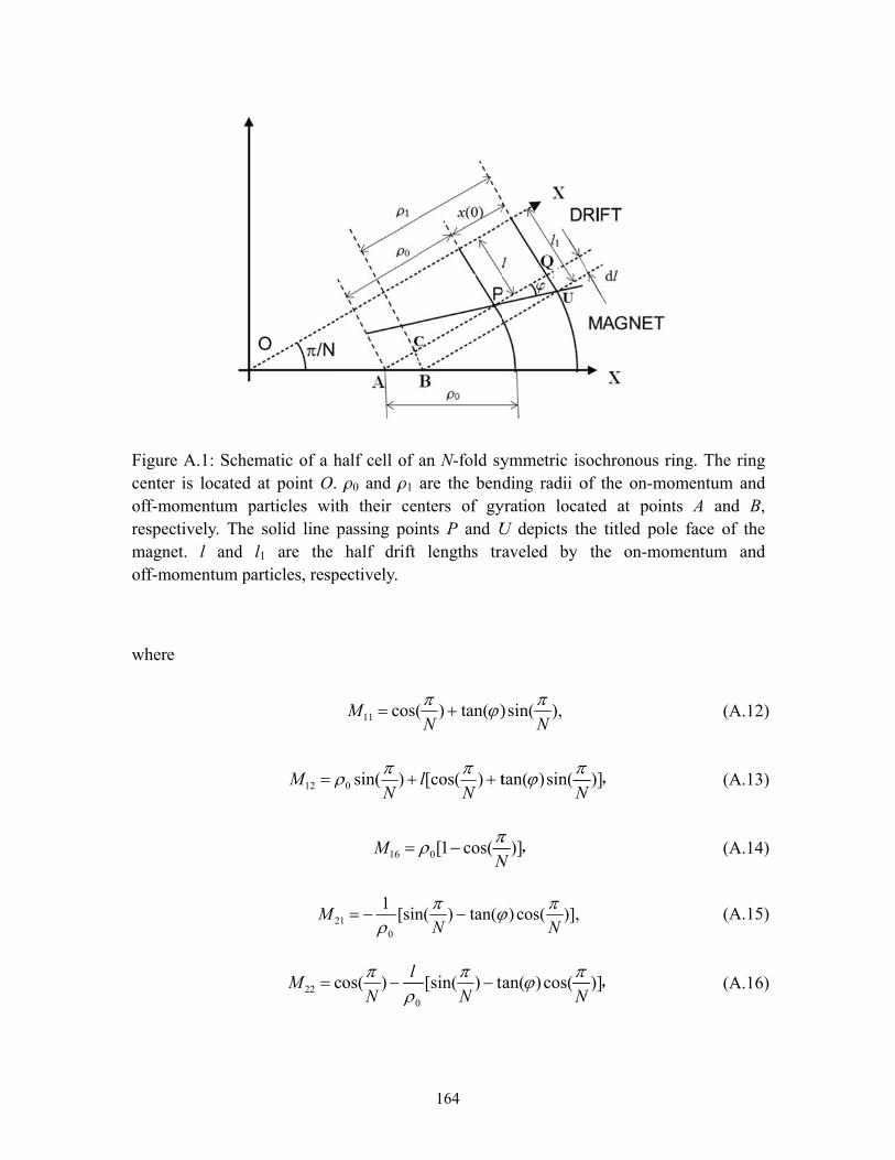
Figurcenteoff-mrespemagnoff-m
wher
re A.1: Scheer is located momentum pectively. Thenet. l and momentum p
e
ematic of a hat point O.
particles wie solid line l1 are the articles, resp
12M
2M
c22M
half cell of . r0 and r1 th their cenpassing poihalf drift
pectively.
cos(11M
)sin(0 N
16M
[sin1
021
)cos(0
l
N
164
an N-fold syare the bendnters of gynts P and Ulengths tra
)tan()(N
t)[cos(N
l
cos(1[0 N
tan()n(N
ta)[sin(0 N
ymmetric isoding radii o
yration locatU depicts thaveled by
),sin()N
sin()tan(N
,)]N
)],cos()N
cos()an(N
ochronous rof the on-moted at poin
he titled polthe on-mo
,)]N
,)]N
ring. The rinomentum annts A and Be face of thmentum an
(A.1
(A.1
(A.1
(A.1
(A.1
ng nd B, he nd
2)
3)
4)
5)
6)
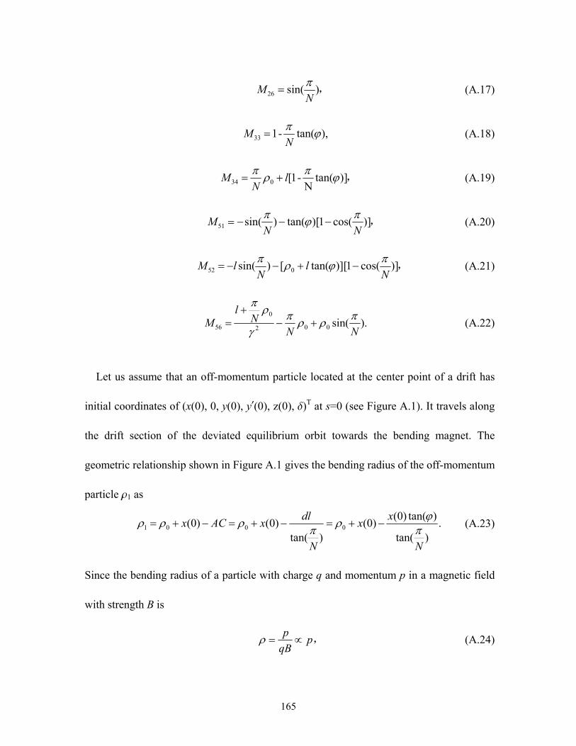
165
,)sin(26 NM
(A.17)
),tan(-133 N
M (A.18)
,)]tan(N
-1[034 l
NM (A.19)
,)]cos(1)[tan()sin(51 NNM
(A.20)
,)]cos(1)][tan([)sin( 052 Nl
NlM
(A.21)
).sin(002
0
56 NNN
lM
(A.22)
Let us assume that an off-momentum particle located at the center point of a drift has
initial coordinates of (x(0), 0, y(0), y£(0), z(0), d)T at s=0 (see Figure A.1). It travels along
the drift section of the deviated equilibrium orbit towards the bending magnet. The
geometric relationship shown in Figure A.1 gives the bending radius of the off-momentum
particle r1 as
.)tan(
)tan()0()0(
)tan()0()0( 0001
N
xx
N
dlxACx
(A.23)
Since the bending radius of a particle with charge q and momentum p in a magnetic field
with strength B is
,pqB
p (A.24)

166
then
,
p
p
00
01 (A.25)
].)tan(
)tan(1[
)0(
0
N
x
(A.26)
According to Eq. (A.11), after traveling a half cell, the longitudinal coordinate of the
off-momentum particle becomes
.)0()0()0( 565251 MzxMxMz (A.27)
If the change of longitudinal coordinate z is 0, e.g.,
,0)0()0()0( 565251 MxMxMzzz (A.28)
then the ring will be isochronous. Since x£(0)=0, Eq. (A.28) reduces to
.0)0()0( 5651 MxMzzz (A.29)
Substituting Eqs. (A.20), (A.22) and (A.26) into Eq. (A.29) gives the isochronous
condition
.
)tan(
)1(
)1()tan(
02
02
02
N
Nl
Nl
(A.30)
For the non-relativistic ions coasting in SIR (gº1), if we replace l by L/2, Eq. (A.30)
reduces to
.
)tan(
2/2/
)tan(
0
N
LL
(A.31)
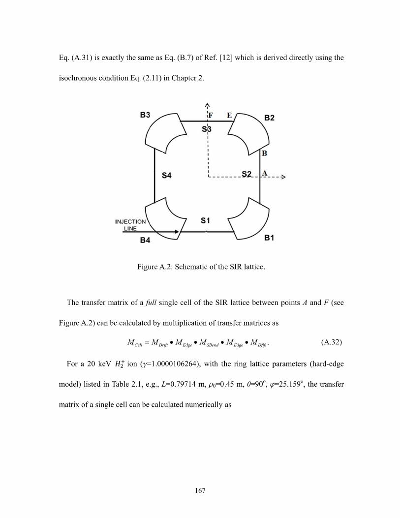
Eq. (A
isoch
Th
Figur
Fo
mode
matri
A.31) is exa
hronous cond
he transfer m
re A.2) can b
r a 20 keV
el) listed in T
ix of a single
actly the sam
dition Eq. (2
Figu
matrix of a fu
be calculated
CellM ion (g=
Table 2.1, e
e cell can be
me as Eq. (B.
.11) in Chap
ure A.2: Sche
ull single ce
d by multipli
EdDrift MM
=1.00001062
.g., L=0.797
calculated n
167
7) of Ref. [1
pter 2.
ematic of the
ll of the SIR
ication of tra
SBenddge M
264), with th
714 m, r0=0
numerically
12] which is
e SIR lattice
R lattice betw
ansfer matric
DfEdge MM
he ring latti
.45 m, q=90
as
derived dire
e.
ween points
ces as
.fift
ice paramete
0o, j=25.159
ectly using th
s A and F (s
(A.32
ers (hard-edg
9o, the transf
he
ee
2)
ge
fer
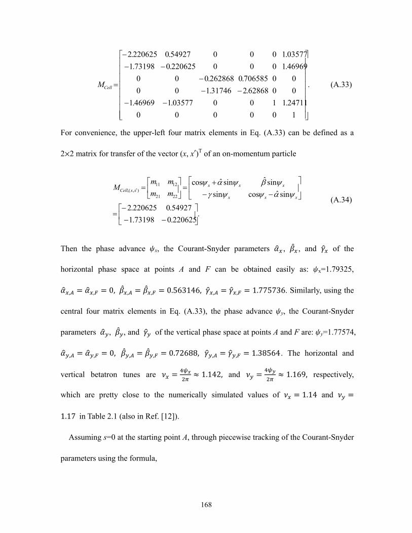
168
.
100000
24711.110003577.146969.1
0062868.231746.100
00706585.0262868.000
46969.1000220625.073198.1
03577.100054927.0220625.2
CellM (A.33)
For convenience, the upper-left four matrix elements in Eq. (A.33) can be defined as a
2μ2 matrix for transfer of the vector (x, x£)T of an on-momentum particle
.220625.073198.1
54927.0220625.2
sinˆcossin
sinˆsinˆcos
2221
1211),(,
xxx
xxxxxCell mm
mmM
(A.34)
Then the phase advance yx, the Courant-Snyder parameters , , and of the
horizontal phase space at points A and F can be obtained easily as: yx=1.79325,
, = , = 0, , = , = 0.563146, , = , = 1.775736. Similarly, using the
central four matrix elements in Eq. (A.33), the phase advance yy, the Courant-Snyder
parameters , , and of the vertical phase space at points A and F are: yy=1.77574,
, = , = 0, , = , = 0.72688, , = , = 1.38564. The horizontal and
vertical betatron tunes are = ≈ 1.142, and = ≈ 1.169, respectively,
which are pretty close to the numerically simulated values of = 1.14 and =1.17 in Table 2.1 (also in Ref. [12]).
Assuming s=0 at the starting point A, through piecewise tracking of the Courant-Snyder
parameters using the formula,
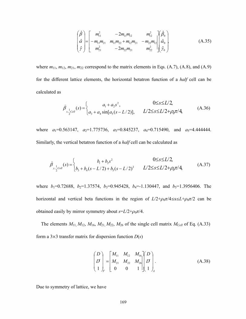
169
,
ˆ
ˆ
ˆ
2
2
ˆ
ˆ
ˆ
0
0
0
2222122
221
1222211222112111
2121211
211
mmmm
mmmmmmmm
mmmm
(A.35)
where m11, m12, m21, m22 correspond to the matrix elements in Eqs. (A.7), (A.8), and (A.9)
for the different lattice elements, the horizontal betatron function of a half cell can be
calculated as
)],2/(sin[
,)(
543
221
2
1, Lsaaa
saas
Cellx
,4/2/2/
,2/0
0
LsL
Ls (A.36)
where a1=0.563147, a2=1.775736, a3=0.845237, a4=0.715490, and a5=4.444444.
Similarly, the vertical betatron function of a half cell can be calculated as
2
543
221
2
1, )2/()2/(
)(LsbLsbb
sbbs
Celly
,4/2/2/
,2/0
0
LsL
Ls (A.37)
where b1=0.72688, b2=1.37574, b3=0.945428, b4=-1.130447, and b5=1.3956406. The
horizontal and vertical beta functions in the region of L/2+r0p/4§s§L+r0p/2 can be
obtained easily by mirror symmetry about s=L/2+r0p/4.
The elements M11, M12, M16, M21, M22, M26 of the single cell matrix MCell of Eq. (A.33)
form a 3μ3 transfer matrix for dispersion function D(s)
.
11001262221
161211
AF
D
D
MMM
MMM
D
D
(A.38)
Due to symmetry of lattice, we have
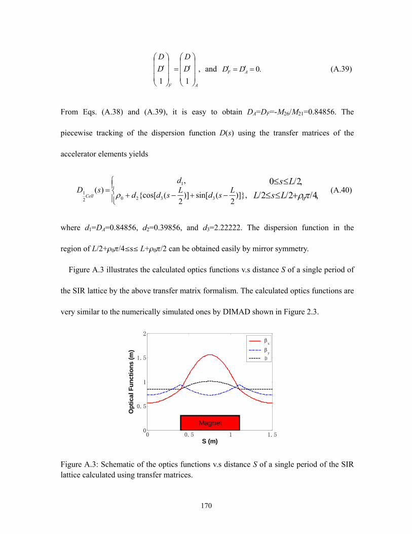
170
,
11AF
D
D
D
D
and .0 AF DD (A.39)
From Eqs. (A.38) and (A.39), it is easy to obtain DA=DF=-M26/M21=0.84856. The
piecewise tracking of the dispersion function D(s) using the transfer matrices of the
accelerator elements yields
)],2
(sin[)]2
(cos[
,)(
3320
1
2
1 Lsd
Lsdd
dsD
Cell ,4/2/2/
,2/0
0
LsL
Ls (A.40)
where d1=DA=0.84856, d2=0.39856, and d3=2.22222. The dispersion function in the
region of L/2+r0p/4§s§ L+r0p/2 can be obtained easily by mirror symmetry.
Figure A.3 illustrates the calculated optics functions v.s distance S of a single period of
the SIR lattice by the above transfer matrix formalism. The calculated optics functions are
very similar to the numerically simulated ones by DIMAD shown in Figure 2.3.
Figure A.3: Schematic of the optics functions v.s distance S of a single period of the SIR lattice calculated using transfer matrices.
0 0.5 1 1.50
0.5
1
1.5
2
Magnet
S (m)
Op
tica
l Fu
nct
ion
s (m
)
x
y
D

171
Using Eqs. (2.5) and (A.40), the average value of dispersion function inside the bending
magnets can be calculated as
.95746.0)(4/
1)(
2
1)(
2
100
bend Cellbendbend dssDdssDsD
(A.41)
Then Eq. (2.6) gives the momentum compaction factor
.9999868.02/)24(
)()(
0
L
sD
R
sD bendbend (A.42)
Finally, the slip factor can be calculated as
.1006.81
- 6-20
(A.43)
In principle, the theoretical value of h0 of the SIR lattice (hard-edge model) should be 0,
the small deviation may originate from the rounding errors and neglect of the relativistic
effects in the numerical calculation.
172
APPENDIX B
TRANSFER MATRIX USED IN CHAPTER 4 AND REF. [42]
The notations of the transfer matrix elements Ri,j (i, j=1, 2,…6) adopted in Chapter 4
follow the ones used in Ref. [42], some of which are different from the standard ones Mi,j
defined in Appendix A of this dissertation. This section is devoted to the comparison of
the two different notations between the two matrices.
B.1 Relations of R51, R52 and R56 between two different matrices
According to Ref. [42], the equations of motion of an ultra-relativistic electron are:
Radial (horizontal): ,xds
dx ,)(
)('
sRxsk
ds
dxx
(B.1)
Longitudinal: ,)(sR
x
ds
dz .0
ds
d (B.2)
where d=Dp/p is the fractional deviation of momentum. The general solution to the
above equations is [42]:
),sinˆcosˆ
(ˆ00
0
0
xx
Dx (B.3)
),cosˆsinˆ
(ˆ
1)
ˆˆ
- 00
0
0
xx
DpxDx ( (B.4)
173
.052051560 xRxRRzz (B.5)
The transfer matrix elements R51, R52, R56 can be obtained from the above equations as
,)(
)()(
056
s
sdsR
sDsR (B.6)
,)(cos)(
)(
ˆ
1)(
00
51
s
sdssR
sDsR
(B.7)
,)(sin)(
)(ˆˆ)(
0052
s
sdssR
ssR
(B.8)
where .)(ˆ
1)(
0
s
sds
s
(B.9)
Ref. [42] defined a 2D Gaussian beam model with an initial equilibrium beam
distribution function
),ˆ(]ˆ2
)ˆ(exp[
2 0
00,
200
20
0,0 zug
xxnf
xx
b
(B.10)
where ),2
exp(2
1)( 2
2
g (B.11)
and u is the chirp parameter which accounts for the correlation between z and d.
(a) For transfer line
At s=0, for a transfer line, the initial values of the dispersion function and its
derivative are D(0)=0, D£(0)=0, the phase advance y(0)=0. From Eqs. (B.3) and (B.4)
we have
174
,)0( 0xx (B.12)
.)0(ˆ)0(ˆ
)0( 00 xxx
(B.13)
The standard transfer matrix M(s) defined in Appendix A gives the transfer of z
).0()0( 5251560 xMxMMzz (B.14)
Plugging Eqs. (B.12) and (B.13) into Eq. (B.14) and comparing the coefficients of x0, 0x ,
and d with those of Eq. (B.5) yields the relation
),()( 5656 sMsR ),()( 5252 sMsR ).0(ˆ/)0(ˆ)()( 525151 MsMsR (B.15)
The relation described in Eq. (B.15) repeats that clarified in the reference list of Ref. [42]
for transfer lines.
(b) For storage rings
For the case of storage rings, though Ref. [42] did not explicitly address the difference
and relation between the standard transfer matrix elements and the ones defined in that
paper, it can be inferred from the formalism and context of the paper. We know that the
beam dynamics of storage rings is different from that of the transfer lines. For example,
the dispersion function D(s) and its derivative D£(s) of storage rings are periodic functions
of s and must satisfy the close orbit condition, e.g., D(s)=D(s+C0), D£(s)=D£(s+C0), where
C0 is the ring circumference. Hence, D(s) and D£(s) of storage rings are self-consistent
solutions of ring lattice optics required by the periodicity. While D(s) and D£(s) of transfer
lines are free from the above restraint.
According to the smooth approximation adopted in Ref. [42] in the derivation of the 2D
175
dispersion relation (e.g., xR /ˆ , Rsx / , 2/ xRD , 0ˆ , 0D and Rxxx /20, ),
at s=0, Eqs. (B.3) and (B.4) yield
,)0( 0 Dxx (B.16)
.)0( 0xx (B.17)
Eq. (B.16) indicates that x0 is the initial betatron oscillation amplitude xb(0), which is
not equal to the total initial radial offset x(0), the latter includes a dispersion term Dd.
Consequently, the first exponential function defined in Eq. (B.10) describes the initial
Gaussian distribution of the betatron oscillation amplitudes x0 and slopes 0x , not x(0) and
slopes );0(x moreover, xxxx R /ˆ0,0, is the RMS beam radius which only
includes the emittance effect, since the total RMS beam radius with dispersion effect
should be .//)(22
0,22
, xxxxtotalx RRD Plugging Eqs. (B.16) and
(B.17) into Eq. (B.14) and comparing the coefficients of x0, 0x , and d with those of Eq.
(B.5) yields the relation of different matrix elements for storage rings
),()()()( 515656 sMsDsMsR ),()( 5252 sMsR ).()( 5151 sMsR (B.18)
B.2 One-turn transfer matrices by smooth approximation
By smooth approximation, the longitudinal and radial equations of motion of a particle
in SIR can be written as
Radial (horizontal): ,)(
)(2
2
2
2
sRxs
R
v
ds
xd x (B.19)
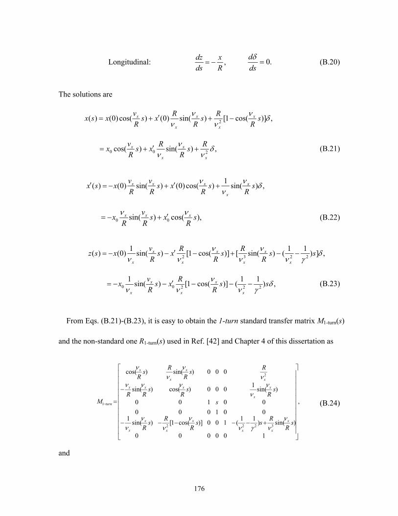
176
Longitudinal: ,R
x
ds
dz .0
ds
d (B.20)
The solutions are
,)]cos(1[)sin()0()cos()0()(2
sR
Rs
R
Rxs
R
vxsx x
x
x
x
x
,)sin()cos(200
x
x
x
x Rs
R
Rxs
R
vx (B.21)
,)sin(1
)cos()0()sin()0()(
s
Rs
Rxs
R
v
R
vxsx x
x
xxx
),cos()sin( 00 sR
xsR
v
Rx xxx (B.22)
,])11
()sin([)]cos(1[)sin(1
)0()(2232
ssR
Rs
R
Rxs
R
vxsz
x
x
x
x
x
x
x
,)11
()]cos(1[)sin(1
22200
ssR
Rxs
R
vx
x
x
x
x
x
(B.23)
From Eqs. (B.21)-(B.23), it is easy to obtain the 1-turn standard transfer matrix M1-turn(s)
and the non-standard one R1-turn(s) used in Ref. [42] and Chapter 4 of this dissertation as
,
100000
)sin()11
(100)]cos(1[)sin(1
001000
00100
)sin(1
000)cos()sin(
000)sin()cos(
3222
2
1
sR
Rss
R
Rs
R
s
sR
sR
sRR
Rs
R
Rs
R
M
x
xx
x
x
x
x
x
x
xxx
x
x
x
x
turn
(B.24)
and
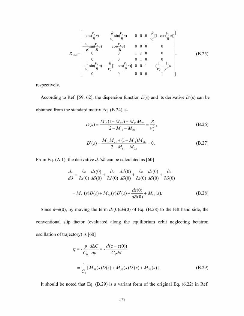
177
,
100000
)11
(100)]cos(1[)sin(1
001000
00100
0000)cos()sin(
)]cos(1[000)sin()cos(
222
22
1
ssR
Rs
R
s
sR
sRR
sR
Rs
R
Rs
R
R
x
x
x
x
x
xxx
x
x
x
x
turn
(B.25)
respectively.
According to Ref. [59, 62], the dispersion function D(s) and its derivative D£(s) can be
obtained from the standard matrix Eq. (B.24) as
,2
)1()(
22211
26122216
x
R
MM
MMMMsD
(B.26)
.02
)1()(
2211
26112116
MM
MMMMsD (B.27)
From Eq. (A.1), the derivative dz/dd can be calculated as [60]
)0()0(
)0(
)0()0(
)0(
)0()0(
)0(
)0(
z
d
dz
z
z
d
xd
x
z
d
dx
x
z
d
dz
).()0(
)0()()()()( 565251 sM
d
dzsDsMsDsM
(B.28)
Since d=d(0), by moving the term dz(0)/dd(0) of Eq. (B.28) to the left hand side, the
conventional slip factor (evaluated along the equilibrium orbit neglecting betatron
oscillation of trajectory) is [60]
dC
zzd
dp
Cd
C
p
00
))0((--
)].()()()()([1
5652510
sMsDsMsDsMC
(B.29)
It should be noted that Eq. (B.29) is a variant form of the original Eq. (6.22) in Ref.

178
[60], which is the expression for momentum faction factor a in the ultra-relativistic limit
instead of slip factor h; in addition, there is no negative sign on the right hand side of Eq.
(6.22) in Ref. [60], because Ref. [60] uses a different sign convention in definition of slip
factor.
With Eqs. (B.24), (B.26) and (B.27) and (B.29), in the end, the slip factor for the
one-turn matrix of a storage ring can be obtained as
.11
22
x
(B.30)
While for the non-standard 1-turn transfer matrix R1-turn(s) in Eq. (B.25), the
conventional slip factor (neglecting the betatron oscillation effect) is related to the matrix
element R56(s) exclusively by
.11
|)(
-22
0
560
x
CsC
sR (B.31)
Particularly, in the case of isochronous rings, the radial (horizontal) tune nx in Eqs. (B.30)
and (B.31) should be replaced by transition gamma gt.

179
BIBLIOGRAPHY

180
BIBLIOGRAPHY
[1] C. Rubbia, et al. “Conceptual design of a fast neutron operated high power energy amplifier” CERN/AT/95-44 (ET).
[2] R. Sheffield, “Utilization of accelerators for transmutation and energy production”, Proc. HB2010, Morschach, Switzerland (2010), p. 1–5.
[3] N. Pogue, et al, “A strong-focusing 800 MeV cyclotron for high-current applications”, AIP Conf. Proc. 1525, pp. 226-229; Application of accelerators in research and industry: Twenty-Second International Conference, Date: 5–10 August 2012, Location: Ft. Worth, TX, USA.
[4] L. Calabretta, et al, “A multi megawatt cyclotron complex to search for CP violation In the neutrino sector”, Proceedings of CYCLOTRONS 2010, Lanzhou, China, p. 298-303.
[5] R. J. Barlow, et al, “High power cyclotrons for the neutrino experiments DAEδALUS and ISODAR”. Proceedings of IPAC2013, Shanghai, China. p. 446-448.
[6] M. Seidel, “Cyclotrons for high-intensity beams”, CERN-2013-001, p. 17-32.
[7] T. Planche, et al, “Space charge effects in isochronous FFAGS and Cyclotrons”, Proceedings of HB2012, Beijing, China, p. 231-234.
[8] P. J. Bryant and K. Johnson, “The principles of circulars accelerators and storage rings” (Cambridge University Press, 1993).
[9] M. M. Gordon, Proceedings of the 5th International conference on Cyclotrons, Oxford, United Kingdom (1969), p. 305.
[10] A. J. Cerfon, J. P. Freidberg, F. I. Parra, T. A. Antaya, Physical Review Special Topics – Accelerators and Beams 16, 024202 (2013).
[11] W. J. G. M. Kleeven and Y.K. Batygin, “Momentum analysis of space charge effects in an AVF cyclotron”, Particle Accelerators 24 (1989), p. 187.
[12] E. Pozdeyev, Ph.D. thesis, Michigan State University (2003).
181
[13] J. A. Rodriguez, Ph.D. thesis, Michigan State University (2004).
[14] E. Pozdeyev, J. A. Rodriguez, F. Marti, R. C. York, Proceedings of Hadron Beam, Nashville, Tennessee, U.S.A (2008), WGA30, p. 157.
[15] E. Pozdeyev, J. A. Rodriguez, F. Marti, R.C. York, Physical Review Special Topics – Accelerators and Beams 5, 054202 (2009).
[16] Y. Bi, T. Zhang, C. Tang, Y. Huang, J. Yang, Journal of Applied Physics, 107, 063304 (2010).
[17] A. Adelmann et al., “The OPAL (Object Oriented Parallel Accelerator Library) framework, users reference manual”, Version 1.2.0, PSI report number PSI-PR-08-02, Paul Scherrer Institut (2008).
[18] J. J. Yang et al., “Beam dynamics in high intensity cyclotrons including neighboring bunch effects: Model, implementation, and application”, Physical Review Special Topics – Accelerators and Beams 13, 064201 (2010).
[19] Y. Li, G. Machicoane, F. Marti, T. P. Wangler, E. Pozdeyev, Proceedings of the IEEE Particle Accelerator Conference (Vancouver, Canada, 2009), TU3PBC06, p. 734.
[20] A. W. Chao, Physics of Collective Beam Instabilities in High Energy Accelerators (John Wiley & Sons, Inc., New York, 1993).
[21] D. A. Edwards, M. J. Syphers, An Introduction to the Physics of High Energy Accelerators (John Wiley & Sons, Inc., New York, 1993).
[22] Z. Huang, M. Borland, P. Emma, J. Wu, C. Limborg, G. Stupakov and J. Welch, Physical Review Special Topics – Accelerators and Beams 7, 074401 (2004).
[23] J. Rosenzweig, C. Pellegrini, L. Serafini, C. Ternienden and G. Travish, TESLA FEL-Report 1996-15.
[24] M. Venturini, LBNL-63111, 2007.
[25] M. Venturini, Physical Review Special Topics – Accelerators and Beams 11, 034401 (2008).
[26] J. Qiang, R. D. Ryne, M. Venturini, A. A. Zholents, I. V. Pogorelov, Physical Review Special Topics – Accelerators and Beams 12, 100702 (2009).

182
[27] S. Humphries, Charged Particle Beams (John Wiley & Sons, Inc., New York, 1990), p. 704.
[28] A. M. Al-khateeb, O. Boine-Frankenheim, Ingo Hofmann, and G. Rumolo, Physical Review E 63, 026503 (2001).
[29] L. Palumbo, V. G. Vaccaro, G. Wustefeld, IEEE Transactions on Nuclear Science, 31 (1984).
[30] W. R. Smythe, Static and Dynamic Electricity (McGraw-Hill Book Company Inc., New York, 1950), p. 85.
[31] C. E. Nelson and A. M. Sessler, Review of Scientific Instruments, 30(02), 1959, p. 80-89.
[32] K.Y. Ng, Particle Accelerators 16 (1984) 63.
[33] B. Zotter, ISR-TH/68-46, 1968.
[34] O. Gröbner and K. Hübner, CERN/ISR-TH-VA/75-27, 1975.
[35] A.V. Smirnov, Nuclear Instruments and Methods in Physics Research A 450 (2000), p. 579-582.
[36] N. Mounet and E. Métral, CERN-ATS-Note-2010-056 Tech, 2010.
[37] R. L. Gluckstern, J. van Zeijts, and B. Zotter, Physical Review E, 47 (1993), p. 656-663.
[38] R. Warnock and R. Ruth, Physical Review Special Topics – Accelerators and Beams 8, 014402 (2005).
[39] See e.g., J. N. Reddy, An Introduction to the Finite Element Method (3rd edition, McGraw-Hill Higher Education, 2006).
[40] X. Lin,Z. Zhang,Solved Problems in Electrodynamics (in Chinese), Science Press, Beijing, ISBN 7030071298 (2002), p. 72.
[41] D. Ratner, Ph.D. thesis, Stanford University (2011).
[42] S. Heifets, G. Stupakov, and S. Krinsky, Physical Review Special Topics–

183
Accelerators and Beams 5, 064401 (2002).
[43] T. J. M. Boyd, J.J. Sanderson, The Physics of Plasmas (Cambridge University Press, Cambridge, 2003), p. 256-260.
[44] P. M. Bellan, Fundamentals of Plasma Physics (Cambridge University Press, New York, 2006), p. 182-192.
[45] N. A. Krall, A. W. Trivelpiece, Principles of Plasma Physics (McGraw-Hill, Inc., New York, 1973), p. 375-380.
[46] C. N. Lashmore-Davies, CERN-81-13, 1981, p. 30-38.
[47] M. Reiser, Theory and Design of Charged Particle Beams (Wiley-VCH Verlag GmbH & Co. KGaA, Weinheim, 2008), p. 190-192.
[48] J. A. Simpson, Review of Scientific Instruments, 32, 1283 (1961).
[49] E. R. Cawthron, D. L. Cotterell, and M. Oliphant, Proceedings of the Royal Society of London A 314, 39-51, (1969).
[50] Y. Zou, Y. Cui, I. Haber, M. Reiser, and P. G. O’Shea, Physical Review Special Topics-Accelerators and Beams, 6, 112801 (2003).
[51] Y. Zou, Y. Cui, V. Yun, A. Valfells, R. A. Kishek, S. Bernal, I. Haber, M. Reiser, and P. G. O’Shea, Physical Review Special Topics-Accelerators and Beams, 5, 000000 (2002).
[52] Y. Cui, Y. Zou, A. Valfells, M. Reiser, M. Walter, I. Haber, R. A. Kishek, S. Bernal, and P. G. O’Shea, Review of Scientific Instruments 75, Number 8 (2004).
[53] SIMION, Scientific Instrument Services, Inc, http://simion.com/.
[54] Lua, http://www.lua.org/.
[55] G. Machicoane, D. Cole, J. Ottarson, J. Stetson, and P. Zavodszky, Review of Scientific Instruments 77, 03A322 (2006).
[56] H. Hamma, H. Tanaka, N. Kumagai, M. Kawai, F. Hinode, T. Muto, K. Nanbu, T. Tanaka, K. Kasamsook, K. Akiyama, and M. Yasuda, New Journal of Physics 8 (2006), p. 292.
184
[57] Y. Bi, et al, “Towards quantitative simulations of high power proton cyclotrons”, Physical Review Special Topics – Accelerators and Beams 13, 054402 (2011).
[58] K. R. Crandall and D. P. Rusthoi, TRACE 3-D Documentation, 3rd edition, LA-UR-97-886, (1997).
[59] M. Conte and W. W. MacKay, An Introduction to the Physics of Particle Accelerators (2nd edition, World Scientific Co. Pte. Ltd, Singapore, 2008).
[60] W. W. MacKay and M. Conte, Accelerator Physics-Example Problems with Solutions (World Scientific Co. Pte. Ltd, Singapore, 2012).
[61] K. L. Brown, SLAC-Report-75, 1982.
[62] S. Y. Lee, Accelerator Physics (2nd Edition, World Scientific Co. Pte. Ltd, Singapore, 2004).