Structural Alignment Methods with Applications to Geospatial

Structural Alignment Methods

with Applications to Geospatial Ontologies

Isabel F. Cruz and William Sunna

Department of Computer Science

University of Illinois at Chicago

Short title: Structural Alignment Methods

Keywords: ontology alignment, geospatial ontologies, data integration, semantic web

Corresponding author: Isabel F. Cruz, Department of Computer Science, University of Illinois

at Chicago, 851 S. Morgan St. (M/C 152), Chicago, IL 60607, USA. E-mail: [email protected].

1

Abstract

We consider the problem of enabling interoperability and information sharing among geospa-

tial applications that use ontologies to describe their concepts and the relationships among them.

We present two fully automatic alignment methods that use the graph structures of a pair of

ontologies to establish their alignment, that is, the semantic correspondences between their con-

cepts. We have tested our methods on geospatial ontologies pertaining to wetlands and four

other pairs that belong to a repository that has been used in the Ontology Alignment Evalu-

ation Initiative (OAEI). Using these ontologies, we have compared the effectiveness (precision

and recall) of our methods against the Similarity Flooding Algorithm that was proposed by

others and show that for each of the tested ontologies one of our methods is at least as effective

as their method. We have tuned the performance of our methods by introducing a greedy ap-

proach that reduces the number of concepts that get compared. This approach reduces runtime

by approximately 30% with a minor compromise to the effectiveness of the results. To further

validate our approach, we participated in the OAEI competition to align a pair of ontologies,

each with a few thousand concepts.

2

1 Introduction

Heterogeneities in geospatial information systems are generally caused by modeling the same aspects

of reality in different ways. This is mainly due to the fact that such systems are developed by

domain experts who have limited or no communication among them. Our focus in this paper

is on classification schemes that are commonly used in geospatial applications such as land use or

wetlands. For example, in the case of land use, there are potentially dozens of different land use data

classifications associated with counties and municipalities, thus hindering land use planning across

the borders of the different jurisdictions (Wiegand et al., 2002). As for wetlands, organizations

monitoring their data inventory have an interest in sharing data. However, the lack of standard

classification has long been identified as an obstacle to the development, implementation, and

monitoring of conservation strategies both at the national and regional levels (Dini et al., 1998).

In other words, data integration, defined as the problem of combining data that resides in different

sources so as to provide users with a unified view over these data (Lenzerini, 2002), becomes only

feasible if correspondences can be established across the different classification schemes that are

associated with one or more geographical areas.

The classification schemes used by geospatial applications are often just syntactic constructs

that assume different formats (for example, tables), where the hierarchical characteristics that

should be inherent to a classification scheme are not always explicitly represented (Wiegand et al.,

2002). Such legacy formats are in sharp contrast with current standardization efforts, such as

the Open Geospatial Consortium, 1 which rely on ontologies to describe the domains of interest.

Ontologies contain a conceptual description of data, consisting of the concepts used, their attributes,

and the relationships between those concepts. In this paper, we model classification schemes as

ontologies. A direct consequence is that hierarchies of concepts can be readily modeled using

“is-a” relationships. In this context, establishing correspondences across classification schemes is

tantamount to ontology matching or alignment in which semantic connections are established among

the concepts of two ontologies: one being the source ontology and the other the target ontology.

Ontologies also play an important role in data integration (Cruz and Xiao, 2005).

Ontology alignment encompasses a wide variety of techniques, which are concept-based, that is,

geared to the matching of single concepts (Bergamaschi et al., 1999; Castano et al., 2001; Palopoli

et al., 1998) or structure-based, that is, taking into account the structural organization of several1http://www.opengeospatial.org/.

3

concepts at a time (Melnik et al., 2002; Noy and Musen, 2001; Rodrıguez and Egenhofer, 2003).

Other approaches are instance-based, that is, they consider data associated with the ontological

concepts (Doan et al., 2002; Fossati et al., 2006; Ichise et al., 2001). In this paper, we concentrate

on the first two techniques.

As ontologies grow in size or in number, their alignment should ideally be automatic or re-

quire minimum user intervention. For this reason, the Ontology Alignment Evaluation Initiative

(OAEI) (Euzenat et al., 2007) promotes the competition of automatic alignment methods in terms

of their effectiveness (recall, precision, and F-measure) and efficiency (runtime). Every year, they

build a repository of ontology sets. Each set contains a source ontology, a target ontology, and

the reference alignment between them, as determined by domain experts. Several of these sets

are released after the competition. This is an important “side effect” of the competition. In fact,

while the number of web available ontologies increases every day, it is the availability of reference

alignments that provides researchers with ways of testing and evaluating their alignment meth-

ods objectively. The effort needed to produce those reference alignments is however considerable,

therefore examples from many domains of interest, such as the geospatial domain, are not currently

available.

In this paper, we present two (fully) automatic structure-based methods: the Descendant’s

Similarity Inheritance (DSI) method, which uses the relationships between ancestor concepts, and

the Sibling’s Similarity Contribution (SSC) method, which uses the relationships between sibling

concepts. In our previous work, we have developed the AgreementMaker system, which incorporates

several alignment methods (Cruz et al., 2002, 2005, 2004) organized in layers. The DSI and SSC

methods have been incorporated in our system.

We have chosen the example of wetlands for our geospatial application domain, because it moti-

vates well the need for structure-based methods. We implemented our proposed methods and tested

them against our previously developed concept-based technique (Cruz et al., 2007), which provides

us with a base case. Users can select a similarity value (threshold) for our concept-based method,

henceforth called base similarity. We have investigated the influence of the choice of the threshold

value in terms of precision and recall. In addition, we tested our methods against the implementa-

tion of an existing structure-based algorithm, the Similarity Flooding (SF) algorithm (Melnik et al.,

2002). Besides the wetlands ontologies, our experiments involve aligning four ontology sets from

the OAEI. Our experiments show that at least one of our structure-based methods is as effective

or better than both our base case method and the SF algorithm.

4

To further validate our approach, we competed in the 2007 Ontology Alignment Evaluation

Initiative (OAEI) competition with the DSI method (Sunna and Cruz, 2007b). In the absence of

the availability of a geospatial track, we competed in a the biomedical track, a “general purpose

track” (in the sense that the alignment methods cannot take advantage of prior knowledge of the

domain) where the objective was the alignment of two large ontologies consisting of a couple of

thousand concepts each. A total of seven alignment systems (including ours) competed in aligning

the biomedical ontologies. The alignment of these ontologies included three test cases whose aim

was respectively to get optimal values for F-measure, precision, and recall. Our system came

respectively in third, fourth, and third places.

Having achieved satisfactory results in aligning the OAEI ontologies, our focus shifted to im-

proving the performance of our automatic algorithms. To this end, we have tuned our methods by

introducing a greedy approach that is selective to what concepts get compared. On average, our

approach reduced runtime by around 30% with a small compromise in the quality of the alignment

results.

This paper extends our previous work (Sunna and Cruz, 2007a) in several ways: we analyze the

influence of the choice of the threshold value in terms of precision and recall; we present the results

obtained in the OAEI 2007 competition; based on the results obtained, we propose a technique

for improving the performance of our method; we study the influence of the improved performance

technique on precision and recall.

The rest of this paper is organized as follows. In Section 2, we give an overview of related work

in the area. We provide further details on the wetland ontologies and on their suitability for testing

structure-based alignment methods in Section 3. We describe briefly our multi-layered approach to

ontology alignment as implemented by our alignment system in Section 4. In Section 5, we describe

the SF algorithm and present our automatic structure-based methods, DSI and SSC, that support

the first layer of our system. We describe the results of applying our methods to five ontology sets

including the wetlands set in Section 6. In Section 7, we discuss the influence of the base similarity

threshold in precision and recall. We present the results of our participation in the 2007 OAEI

competition in Section 8. In Section 9, we present our methodology for enhancing the performance

of our automatic methods and the results of applying this enhancement to the alignment of the

OAEI ontology sets. Finally, in Section 10, we draw conclusions and outline future work.

5

2 Related Work

In their survey paper, Shvaiko and Euzenat (Shvaiko and Euzenat, 2005) provide a comparative

review of recent schema and ontology matching techniques, which they classify as concept- or

structure-based (respectively, element-level or structure-level in their terminology). In the concept-

based category, the techniques are, for example, string-based (e.g., edit-distance), language-based

(e.g., tokenization), constraint-based (e.g., types, attribute cardinality) or use linguistic resources.

An example of the last include the use of domain specific thesauri or of common knowledge thesauri,

for example, a lexical database such as WordNet. 2 The use of a resource that is not included in the

ontologies to align, such as the use of thesauri, make a technique external (as opposed to internal). In

the structured-based category, the techniques are, for example, graph-based (e.g., based on node or

graph comparisons), taxonomy-based, which are based on particular kinds of relationships between

the nodes (e.g., “is-a” relationships), or model-based, which are based on model theoretic semantics

(e.g., description logic reasoning techniques). Their survey considers that concept-based techniques

are not semantic, because “semantics is usually given in a structure,” however, we consider the use

of semantically organized thesauri such as WordNet to be semantic. Likewise, we consider the

taxonomy-based techniques as semantic, given the semantics associated with relationships among

components in a taxonomy.

The alignment techniques that we describe in this paper are either concept- or structure-based.

In particular, our word comparison is both language-based and linguistic, the latter being both

external and semantic. Our structure-based techniques are graph-based and because of our the

taxonomic nature of our ontologies are also taxonomy-based. In the rest of this section, we outline

several ontology matching approaches and systems and describe also related work on measuring

similarity of ontological structures.

OLA (Owl-Lite Alignment) is an alignment tool for ontologies expressed in OWL (Euzenat et al.,

2005). OLA first builds graphs from the ontologies and then applies a similarity model between

concepts of the ontologies being aligned (Euzenat and Valtchev, 2004), which uses concept-based

(string comparison and lexical comparison using WordNet) and structure-based techniques and

supports both manual mappings and automated mappings. OLA tries to achieve the highest level

of automation, by letting users provide a minimal set of parameters at the initial steps of the

alignment process and then leaving it to the tool to end the alignment. Similarly to our approach,2http://www.wordnet.com.

6

they consider contributions of the neighbors (but only in the case of neighbors of the same type).

Given the emphasis of OLA on OWL, it is difficult to compare our approach with theirs. For better

results their approach needs to be semi-automatic, whereas our approach is designed to be fully

automatic and can take advantage of the graph structure being a tree.

RiMOM (Risk Minimization based Ontology Mapping) uses conditional probabilities to model

the mappings between two concepts and based on them defines candidate mappings. Finding

the optimal mapping is formalized as finding the “action with minimal risk” (Tang et al., 2006).

RiMOM considers both metadata and instances. For each possible mapping category (e.g., string-

based, taxonomy-based) they discover the optimal mappings independently of the other categories.

Finally, they combine the results obtained for the different categories, by creating a combined value

for each candidate mapping. The system can be run in an automatic or semi-automatic mode

and uses an iterative process to arrive at a final mapping table. The mapping categories include

string-based (edit-distance), lexical (including NLP techniques), constraint-based, linguistic (using

a lexical and a statistical similarity dictionaries). As for structure-based techniques, they use a

taxonomic approach. However, they appear to only consider the immediate super- and sub-concepts

of a node.

Another approach for ontology alignment proposes the use of different mapping agents that

establish semantic bridges between the concepts in the source and target ontologies (Silva et al.,

2005). When conflicts arise, they are solved by a negotiation process among the agents. This ne-

gotiation takes into account the confidence values evaluated for each semantic bridge and the effort

associated with the change on those values due to the negotiation process. In our AgreementMaker

system (Cruz et al., 2007), which is formed of several layers that support different alignment meth-

ods, it is up to the final layer, the consolidation mapping layer to apply a priority scheme that is

set by the domain expert, so as to solve conflicts among mappings produced by the different layers.

The Similarity Flooding algorithm is a structural technique, which can be used in matching

a variety of data structures, called models (Melnik et al., 2002). Models can be data schemas,

data instances, or a mixture of both. In their approach, models are converted to directed labeled

graphs. For their algorithm to work, they rely on the fact that concepts from the two graphs are

similar when their adjacent concepts on the graphs are similar. The algorithm starts by obtaining

initial mappings between concepts in the two input graphs using a string matching function that

returns initial similarities between matched concepts. Having established the initial mappings,

the algorithm proceeds iteratively to establish more mappings between other concepts based on

7

the assumption that whenever any two concepts in the input models match with some similarity

measure, the similarity of their adjacent concepts increases. The iterations continue “flooding” the

similarities across the concepts in the graphs until a fixed point is reached where similarity measures

for all concepts have been stabilized. Of the matching techniques that we surveyed, this one is the

closest to our vision of what a structure level approach should be, hence we have implemented their

algorithm so as to compare its results with those of the methods that we propose in this paper.

The subject of measuring similarity of ontological structures (and of proposing metrics for

this purpose) is related to the problem of ontology alignment. However, methods for measuring the

similarity of ontologies return a value and methods for ontology alignment return a set of alignments

between concepts. Having stated this difference, both methods need to establish comparisons

between concepts. Next, we describe briefly three methods for measuring similarity of ontological

structures, which hold similarities with the methods we use.

The first similarity method compares hierarchical ontologies and considers concepts and re-

lations, using the notion of semantic cotopy, which, given a concept, returns all its super- and

sub-concepts, thus taking into account the structure of the ontologies (Maedche and Staab, 2002).

However, there is no amortized effect depending on the distance of those concepts. The second

similarity method proposes an even more comprehensive similarity method that combines two

components: lexical and taxonomic (which also uses the semantic cotopy notion) (Dellschaft and

Staab, 2006). The third similarity method converges even for cyclic ontologies (as is the case with

the SF algorithm) such as those that may occur when OWL-Lite is used (Euzenat and Valtchev,

2004).

3 Geospatial Application

In this section, we describe a geospatial application for wetlands, which provides the motivation for

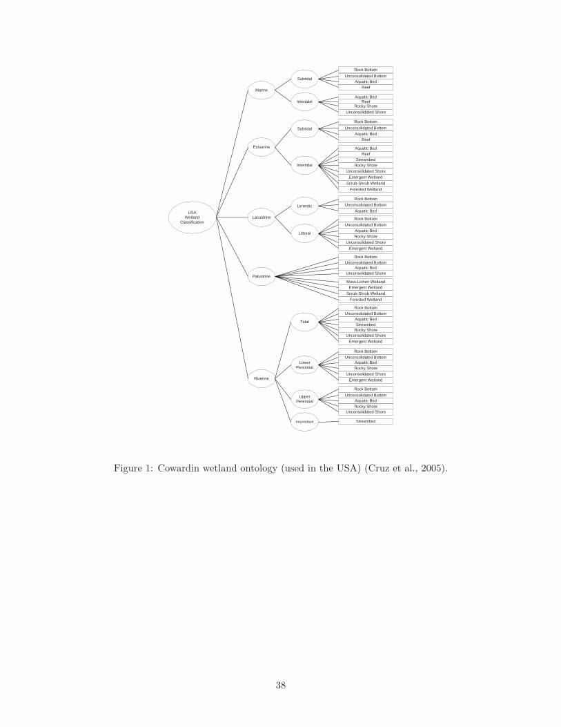
performing structure-based alignment between ontologies. In defining wetlands, the United States

adopts the Cowardin Wetland Classification System (Cowardin et al., 1979). In contrast, European

nations use the International Ramsar Convention Definition (www.ramsar.org) and South Africa

uses the National Wetland Classification Inventory (Dini et al., 1998). Because of the need for

regionalization, it is difficult to have a standardized classification system between nations and also

between regions of a country with a large geographic area (Cowardin et al., 1979).

[ Figure 1 to be placed about here. ]

8

Figure 1 shows the Cowardin Wetland Classification System. As can be seen from the figure,

there are several leaves in this hierarchy that are similar, even if their ancestor nodes are different.

A similar observation can be made about the classification schemes for other wetlands systems.

Therefore, one of the main challenges in aligning automatically any two wetland ontologies is

the possibility of producing misleading mappings between concepts with the same name, which

are however classified under non-corresponding categories. That is, establishing base similarities

between concepts of the source ontology and concepts of the target ontology will not be sufficient to

achieve a high degree of precision in relating concepts in the two ontologies. We illustrate further

this point with Figure 2, where the source ontology (on the left) describes part of the Cowardin

classification system and the target ontology (on the right) describes part of the South African

classification system. When calculating the base similarities between concepts of the two ontologies,

the concept Reef that belongs to the Intertidal wetlands subsystem in the source ontology, will

yield a base similarity measure of 100% relative to the concept Reef that belongs to the Intertidal

wetland subsystem in the target ontology. Furthermore, it will also yield a base similarity measure

of 100% with the concept Reef that belongs to the Subtidal wetlands subsystem in the target

ontology. However, if we consider the ancestors of the nodes, hence the structure of the graph, we

will be able to find the correct mappings.


4 AgreementMaker Framework

We have been working on a framework that supports the alignment of two ontologies (Cruz et al.,

2002, 2005, 2004, 2007). In our framework, we incorporate several alignment techniques. Each

technique is embedded in a mapping layer (Cruz et al., 2007). Our mapping layers use concept-based

alignment techniques (first layer) and structure-based alignment techniques (first and third layers).

In addition, domain experts can use their knowledge and contribute to the alignment process in the

manual layer (second layer) and in the deductive layer (third layer). In the third layer, alignments

are automatically propagated along the ontologies using deductive rules, but manual input is needed

when the process stops (Cruz et al., 2004). The fourth layer applies a priority scheme that is set

by the domain expert, so as to solve conflicts among alignments produced by the different layers.

The base similarity method and the structure-based methods were incorporated in the first layer.

The motivation behind our multi-layer framework is to allow for the addition of as many mapping

9

layers as possible in order to capture a wide range of relationships between concepts.

We have developed a system, the AgreementMaker, which implements our approach. It maps

ontologies expressed in XML, RDFS, OWL, or N3. The user interface of the AgreementMaker

displays the two ontologies side by side as shown in Figure 3, which are in this case two land use

ontologies.


After loading the ontologies, the domain expert can start the alignment process by mapping

corresponding concepts manually or invoking procedures that map them automatically (or semi-

automatically). The mapping information is displayed in the form of annotated lines connecting the

matched nodes. There are two types of annotations: textual, which describe the type of mapping

(e.g., exact, subset, superset), and numerical, which capture the similarity between the related

concepts (e.g., 75%). The color of the lines represents the mapping layers that generate them (e.g.,

blue for the first layer, green for the second layer). The user decides what colors are assigned to

which layers. To increase the clarity of the display, the user can specify a similarity threshold so

that only the lines that have similarity values greater or equal to a selected threshold are displayed.

In addition, a maximum number of lines (as associated with each concept) can be specified. The

display of all the mappings that are obtained by the different layers can also lead to cluttering of

the display. To further improve readability, we allow users to hide the results of any of the mapping

layers and to redisplay them as desired.

Many choices were considered in the process of displaying the ontologies and their relation-

ships (Cruz et al., 2007). We have extensively tested our user interface with GIS specialists who

are knowledgeable of land use problems.

5 Automatic Similarity Methods

In order to achieve a high level of confidence in performing the automatic alignment of two ontolo-

gies, a thorough understanding of the concepts in the ontologies is highly desired. To this end, we

propose methods that investigate the ontology concepts prior to making a decision on how they

should be mapped. We consider not only the labels and definitions of the ontology concepts, but

also the relative positions of the concepts in the ontology tree. In the first mapping layer, the user

can select one of the following three matching methods: (1) base similarity only; (2) base similarity

followed by the Descendant’s Similarity Inheritance (DSI) method; (3) base similarity followed by

10

the Sibling’s Similarity Contribution (SSC) method. Both the DSI and the SSC methods, which

are structure-based, have been introduced to enhance the alignment results that were obtained

from using the base similarity method, which is concept-based (Cruz et al., 2007). Any other base

similarity could have been used here (Resnik, 1995; Lin, 1998), but we would like to point out

that our emphasis is on structure-based algorithms and on how they can improve upon a concept-

based method. Therefore, we have used our own base similarity method as the first step to all the

structure-based algorithms we consider, including the Similarity Flooding algorithm of Melnik et

al. (Melnik et al., 2002).

5.1 Base similarity method

The very first step in our approach is to establish initial mappings between the concepts of the

source ontology and the concepts of the target ontology. This is achieved by using a similarity

function and applying it to two concepts (one in each ontology). If the returned value is greater or

equal to a threshold set up by the domain expert, then the two concepts match. The base similarity

value is semantic in that it is determined with the help of a dictionary.

In what follows, we present the details of finding the base similarity between a concept in the

source ontology and a concept in the local ontology:

• Let S be the source ontology and T be the target ontology.

• Let C be a concept in S and C ′ be a concept in T.

• Use function base sim(C, C ′) that yields a similarity measure M, such that 0 ≤ M ≤ 1.

• Given threshold value TH, C ′ is matched to C when base sim(C, C ′) ≥ TH.

• For every concept C in S, define the mapping set of C, denoted MS (C), as the set of concepts

C ′ in T that are matched to C (i.e., base sim(C, C ′) ≥ TH).

The following steps determine the similarity between two concepts C and C ′ by looking at their

labels, label(C) and label(C ′):

• If label(C) is identical to the label(C ′), then return a similarity of 1.

• Else, apply the treat string function on label(C) and label(C ′); this function separates a com-

posite string that contains multiple words into its components. For example, in an ontology

11

that contains concepts related to types of weapons, if label(C)= “air-to-air-missile”, then

the string of the label will be converted to “air to air missile” after applying the func-

tion. Similarly, if label(C) = “ServerSoftware” in an ontology that contains concepts related

to computers and networks, it will be converted to “Server Software” after applying the

treat string(label(C)) function. The function also takes care of words separated by under-

score “ ” characters.

• After applying the treat string function to label(C) and label(C ′), check if the two resulting

labels are identical; if true, return a similarity measure of 1, else proceed to the next step.

• Remove all “Stop words” (such as, “the”, “a”, “to”) from label(C)and label(C ′).

• Retrieve the definitions of every remaining word in the labels from the WordNet dictionary.

For label(C), concatenate the definition of all the words that make up the label into the string

D. For label(C ′), concatenate the definitions of all the words that make up the label into the

string D′.

• Apply the stemming algorithm (Hull, 1996) on every word in D and D′. On a high level,

the algorithm traces words back to their roots, for example it reduces the words “directed”

and “directing” to “direct” and “direct” respectively. In this way, the two words become

comparable to each other.

• Let len(D) be the number of words in the string D, len(D′) be the number of words in the

string D′, and common count(D, D′) be the number of unique common words between D

and D′. Then, compute base sim(C, C ′) as: 2×common count(D,D′)len(D)+len(D′) . For example, the words

“apple” and “orange” share just two words in their definitions, namely “fruit” and “yellow”

and they have respectively 10 and 5 words in their definitions, therefore their base similarity

is 0.27. The definitions of the words “car” and “automobile” are identical in the dictionary,

therefore the base similarity value is 1.

• If base sim(C, C ′) ≥ TH, then add C ′ to MS (C).

Our geospatial example of Section 3, which was illustrated in Figure 2 points to the need to con-

sider not only nodes in isolation but to take into account the structure of the taxonomies involved.

The following two methods reconfigure the base similarity between concepts based respectively on

the concepts of which these nodes are descendants or siblings in the taxonomy.

12

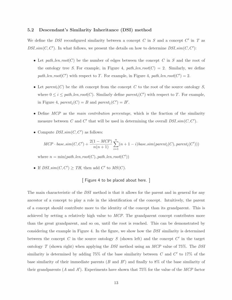
5.2 Descendant’s Similarity Inheritance (DSI) method

We define the DSI reconfigured similarity between a concept C in S and a concept C ′ in T as

DSI sim(C, C ′). In what follows, we present the details on how to determine DSI sim(C, C ′):

• Let path len root(C) be the number of edges between the concept C in S and the root of

the ontology tree S. For example, in Figure 4, path len root(C) = 2. Similarly, we define

path len root(C ′) with respect to T . For example, in Figure 4, path len root(C ′) = 2.

• Let parenti(C) be the ith concept from the concept C to the root of the source ontology S,

where 0 ≤ i ≤ path len root(C). Similarly define parenti(C ′) with respect to T . For example,

in Figure 4, parent1(C) = B and parent1(C ′) = B′.

• Define MCP as the main contribution percentage, which is the fraction of the similarity

measure between C and C ′ that will be used in determining the overall DSI sim(C, C ′).

• Compute DSI sim(C, C ′) as follows:

MCP · base sim(C, C ′) +2(1 − MCP)

n(n + 1)

n∑

i=1

(n + 1 − i)base sim(parenti(C), parenti(C′)))

where n = min(path len root(C), path len root(C ′))

• If DSI sim(C, C ′) ≥ TH, then add C ′ to MS (C).


The main characteristic of the DSI method is that it allows for the parent and in general for any

ancestor of a concept to play a role in the identification of the concept. Intuitively, the parent

of a concept should contribute more to the identity of the concept than its grandparent. This is

achieved by setting a relatively high value to MCP. The grandparent concept contributes more

than the great grandparent, and so on, until the root is reached. This can be demonstrated by

considering the example in Figure 4. In the figure, we show how the DSI similarity is determined

between the concept C in the source ontology S (shown left) and the concept C ′ in the target

ontology T (shown right) when applying the DSI method using an MCP value of 75%. The DSI

similarity is determined by adding 75% of the base similarity between C and C ′ to 17% of the

base similarity of their immediate parents (B and B′) and finally to 8% of the base similarity of

their grandparents (A and A′). Experiments have shown that 75% for the value of the MCP factor

13

works well (in fact, any values in that neighborhood performed similarly). The following example

illustrates just one such case.

Considering the case of Figure 2, the base similarity between the concepts Intertidal in the source

ontology and the concept Subtidal in the target ontology is 37%. The base similarity between the

concepts Marine in the source ontology and the concept Marine in the target ontology is 100%.

When applying the DSI method with an MCP value of 75%, the DSI similarity between the concept

Reef that belongs to the Intertidal wetland subsystem in the source ontology and the concept Reef

that belongs to the Subtidal wetland subsystem in the target ontology will be 88%. Applying the

DSI method again between the concept Reef that belongs to the Intertidal wetland subsystem in

the source ontology and the concept Reef that belongs to the Intertidal wetland subsystem in the

target ontology will yield a similarity of 100%. Therefore, we conclude that the last match is the

best one (in fact the optimal one). This is just one example that shows how the DSI method can

be useful in determining more accurate similarity measures between concepts.

5.3 Sibling’s Similarity Contribution (SSC) method

In this method, siblings of a concept contribute to the identification of the concept. This may

further enhance the quality of the automatic alignment process. Similarly to the DSI method, the

SSC method reconfigures the base similarities between concepts. We define the SSC similarity

between a concept C in S and a concept C ′ in T as SSC sim(C, C ′). In what follows, we present

the details on how to determine this similarity.

• Let sibling count(C) be the number of sibling concepts of concept C in S. For example, in

Figure 5, sibling count(C) = 2.

• Let sibling count(C ′) be the number of sibling concepts of concept C ′ in T . For example, in

Figure 5, sibling count(C ′) = 3.

• Let SS(C) be the set of all the concepts that are siblings of C in S and SS(C ′) be the set of

all the concepts that are siblings of C ′ in T .

• Let Si be the ith sibling of concept C where Si ∈ SS(C), and 1 ≤ i ≤ sibling count(C).

• Let S′j be the jth sibling of concept C ′ where Sj ∈ SS(C ′), and 1 ≤ j ≤ sibling count(C ′).

• Define MCP as the main contribution percentage, which is the fraction of the similarity

measure between C and C ′ that will be used in determining the overall SSC sim(C, C ′).

14

• If both SS(C) and SS(C ′) are not empty, define SSC sim(C, C ′) as follows:

MCP · base sim(C, C ′) +1 − MCP

n

n∑

i=1

max(base sim(Si, S′1), . . . , base sim(Si, S

′m))

where n = sibling count(C) and m = sibling count(C ′).

• If SSC sim(C, C ′) ≥ TH, then add C ′ to MS (C).


The main characteristic of the SSC method is that it allows for the siblings of a given concept to

play a role in the identification process of the concept. In Figure 5 we show how the SSC similarity

is determined between the concept C in the source ontology S (shown on the left) and the concept

C ′ in the target ontology T (shown on the right) when applying the SSC method with an MCP

value of 75% . The SSC similarity is determined by adding 75% of the base similarity between C

and C ′ to (1) 12.5% of the maximum base similarity between D and D′, D and E′, and D and F ′

and to (2) 12.5% of the maximum base similarity between E and D′, E and E′, and E and F ′.

Like for the DSI method, the value of 75% for the MCP factor was found to work well in practice.

5.4 Similarity Flooding algorithm

The Similarity Flooding (SF ) exploits the structure of the schemas to establish correspondences

between their elements (Melnik et al., 2002). We describe briefly how it works. First, the two input

schemas are converted into directed labeled graphs as shown in the example of Figure 6.


Initial correspondences between the elements of the two graphs are established using string matching

techniques. Let us assume that given the similarity values found, correspondences between pairs of

values were established as follows: (S1, T1), (S2, T2), (S3, T2), and (S2, T3).

Following this initial step, a pairwise connectivity graph is derived as shown in Figure 7.


The graph contains nodes that represents the matching pairs, which are connected according to

the structural relationships in the original input graphs. For example, the node representing the

correspondence between S1 and T1 is connected to the node representing the correspondence

15

between S2 and T2 because S1 is connected to S2 in the source input graph, and T1 is connected

to T2 in the target input graph. The SF algorithm proceeds by propagating similarity values

between neighbors in multiple iterations. Each node in the graph divides its propagated similarity

values equally among its neighbors. For example, in Figure 7, (S1, T1) propagates half of its

similarity to (S2, T2) and the other half to (S3, T2). Since node (S2, T2) has only one neighbor

(S1, T1), all of its similarity value is propagated to it. After this process, the similarities that

accumulate at each node get normalized by dividing them by the maximum similarity value in the

graph. This process is repeated until a least fixed point is reached.

6 Experimental results

To validate our approach from the point of view of effectiveness and efficiency, we have aligned the

two wetlands ontologies mentioned in Section 3 using our own methods: base similarity, DSI, and

SSC. We have also used our implementation of the Similarity Flooding algorithm (Melnik et al.,

2002). In addition, to further evaluate our methods, we run experiments on the alignment of four

sets of ontologies provided by the Ontology Alignment Evaluation Initiative (OAEI) (Sure et al.,

2004). Of these, the first set contains two ontologies describing classifications of various weapon

types, the second set contains two ontologies describing attributes of people and pets, the third

set contains two ontologies describing classifications of computer networks and equipments, and

the fourth set contains general information about Russia. Each set contains a source ontology, a

target ontology, and the expected alignment results between them. Table 1 displays the depth and

number of concepts in the five ontology sets we consider.

[ Table 1 to be placed about here. ]

We conducted experiments to determine the efficiency (runtime) of the four methods (base

similarity, DSI, SSC, and Similarity Flooding) for the previously mentioned five ontology sets. We

have implemented all the methods using Java on a 1.6 GHz Intel Centrino Duo with 1GB of RAM,

running Windows XP. The results are shown in Table 2.

The runtime for the DSI, SSC, and Similarity Flooding algorithms include the runtime for the

base similarity method, because that method is run first in all cases. Therefore, the base similarity

algorithm takes the least amount of time. Examining the remaining results, the DSI method has

the best runtime performance for four of the test cases, while the Similarity Flooding algorithm has

16

the best runtime performance for one test case only. The SSC method has the worst performance

in three test cases while it performs better than the Similarity Flooding algorithm in two test

cases. The SSC method depends on the number of siblings for a given concept, therefore the larger

the number of siblings the worse it performs. In other words, if the ontology trees are wide, then

the performance of SSC will suffer. Similarly, the runtime of the DSI method degrades for deep

ontology trees. In Section 9, we present a greedy algorithm that enhances the performance of our

methods.

To compare the effectiveness of the four methods, we started by aligning the set of ontologies for

the wetlands as described in Section 5.2 and did the same for the other four sets of ontologies. In

the wetlands example, we have captured the number of discovered relations between the concepts

of the source ontology (Cowardin) and the concepts of the target ontology (South African) for each

method. Each relationship represents a mapping from a concept C in the source ontology S to a

target ontology concept C ′ ∈ MS (C) with the highest similarity measure. We note that there may

be concepts in S that are not mapped to any concepts in the target ontology (corresponding to an

empty mapping set). Also, there may be more than one concept in S that maps to the same concept

C ′. After capturing the discovered relations, we count how many of these relations are valid when

compared with the expected alignment results. Having determined the number of valid relations,

we calculate both the precision and recall values. Precision is calculated by dividing the number

of discovered valid relations by the total number of discovered relations and recall is calculated by

dividing the number of discovered valid relations by the total number of valid relations as provided

by the expected alignment results.

In the alignment of the wetland ontologies, the DSI method yielded slightly higher precision and

recall values than the Similarity Flooding algorithm which in turn yielded higher values than the

SSC method. Overall, these three methods significantly enhanced the precision and recall values

obtained by applying the base similarity method only. Table 3 shows the complete results for this

test case.

The following tests pertain to the four sets of ontologies of the OAEI initiative. In the alignment

of the ontologies in the first OAEI set (weapons), the DSI method yielded slightly higher precision

and recall values than both the SSC and the Similarity Flooding methods as shown in Table 4.

All four methods yielded the same results for recall and precision in the alignment of the second

OAEI set (people and pets) as shown in Table 5. This is an indication that the locality of all the

concepts in the ontologies of the second set are irrelevant in distinguishing their identity.

17

The SSC method yielded better recall and precision results than the Similarity Flooding algo-

rithm, which in turn yielded better results the the DSI method when aligning the third OAEI set

(computer networks) as shown in Table 6. Finally, as shown in Table 7, in the alignment of the

fourth OAEI set (Russia), the DSI method yielded the highest results for precision and recall than

either the SSC method or the Similarity Flooding algorithm.

The differences found in the recall and precision values for a given method when applied across

different test cases are mainly due to the characteristics of the ontologies. For example, in the

first OAEI set (weapons) and the second OAEI set (people and pets), the relations between the

concepts, their parents, and their siblings do not contribute to refining the base similarity results.

However, the relationships between the concepts and their siblings added value in refining the base

similarity results when aligning the third OAEI set (computer networks). The relationships between

the concepts and their parents added value in refining the results when aligning the fourth OAEI

set (Russia). Therefore, the selection of an appropriate matching method should be done after a

preliminary examination of the concepts in the ontologies and how they relate to each other. A

methodology on how to select an appropriate matching method for a specific alignment has been

proposed, where a domain expert fills out a questionnaire about the nature of the ontologies to be

aligned (Mochol et al., 2006).

7 Precision and Recall Optimization

One feature of our system is the ability to specify a similarity threshold when using the automatic

methods in our first layer of mapping as discussed in Section 5.1. This feature can help the user in

controlling the precision and the recall values during the alignment process. In general, selecting a

relatively high similarity threshold value reduces the number of discovered relations because only

relations that have a high degree of confidence detected by their similarity measures are considered

in the final alignment results. As a result, precision is more likely to increase because it is calculated

by dividing the number of valid discovered relations by the number of discovered relations. Recall,

on the other hand, is more likely to decrease or stay stable because it is calculated by dividing the

number of valid discovered relations by the number of expected valid relations, which is always the

same regardless of the similarity threshold. The reason for a potential decrease in recall when the

similarity threshold is set high, is the possibility of excluding valid relations that yielded similarity

measures below the set similarity threshold. These relations are needed to drive recall higher since

18

the total number of discovered relations does not play a role in calculating recall.

When the user selects lower similarity threshold values, the potential of discovering more rela-

tions increases. As a result, the number of valid discovered relations generally goes up along with

the number of invalid discovered relations, thus generally causing precision to decrease. Recall,

on the other hand, generally improves since it only takes into account the number of valid discov-

ered relations (which has increased) and the number of expected valid relations (which remains

constant).

We have performed experiments that measure the impact of changing the threshold values on

both precision and recall when aligning the four OAEI ontologies. In our experiments, we ran the

base similarity method with five threshold values (20%, 40%, 60%, 80%, and 90%) when aligning

the four ontologies. We also repeated the same experiment with both our DSI and SSC methods.

All the three methods exhibited the same behavior on precision and recall, as far as the impact of

similarly threshold is concerned. The final results of using the three methods in our experiments

were consolidated by averaging the recall and precision values for each of the five aforementioned

similarity threshold values.

Figure 8 shows how the precision and recall values change with different similarity thresholds

in the alignment of the ontologies for weapons. In the figure, we notice a very slight decrease of

the recall and a very slight increase of the precision as the similarity threshold increase.


In aligning the ontologies for people and pets, we notice an increase in precision and a very

slight decrease in recall as the similarity threshold increases, as shown in Figure 9.


In aligning the computer networks ontologies, we notice a sharp increase in precision when the

threshold is set higher than 40%, which is accompanied with a sharp decrease in recall as shown in

Figure 10.


Precision reached its maximum value at threshold values of 80% and above while recall continued

to decrease. Similar behavior is also noticed when aligning the ontologies on Russia as shown in

Figure 11.

19


In conclusion, our approach gives flexibility to the user to steer the automatic alignment in favor

of optimizing recall or precision. The choice is dependent on the purpose of the alignment process.

For example, if the alignment results contribute to an information retrieval system that aims to find

the maximum number of possible correspondences regardless of their correctness, then recall can

be optimized. If the alignment results are used in a more rigid environment where correspondences

are expected to be as much as possible correct, then precision must be optimized.

8 2007 Ontology Alignment Campaign

To further validate our approach, we competed in the 2007 Ontology Alignment Campaign (Eu-

zenat et al., 2007) with our DSI method. We participated in the biomedical anatomy track. The

biomedical anatomy track is considered a “blind test” in that the results of the alignment, which

are contained in a reference alignment document, are hidden from the participants. The reference

document contained only equivalence correspondences between concepts of the ontologies. The

first ontology in this track described the mouse adult anatomy published by the Mouse Gene Ex-

pression Database Project. The second ontology described the human anatomy published by the

National Cancer Institute. The first ontology contained 2744 concepts whereas the second ontology

contained 3304 concepts. In this track, our system competed against six other systems, which, like

ours, can match ontologies in any domain. The quality of the alignments was determined based

on the obtained precision (number of discovered valid relations by the total number of discovered

relations), recall (number of discovered valid relations to the total number of valid relations), and

F-measure (two times the product of precision and recall by their sum).

This track included three test cases, whose aim was respectively to get optimal values for F-

measure, precision, and recall. In the first test case, our system came in third with an F-measure

value of 59.4% (average was 52.6% for all the competing systems), a precision value of 55.8%, and

a recall value of 63.5%. The F-measure reflects a balance between both precision and recall. In

order to obtain a reasonable F-measure value, we set the similarity threshold to 60%. This value

was selected moderately (somewhere between 0% and 100%) in order to prohibit the establishment

of any weak correspondences to optimize recall but so as to allow for stronger correspondences to

be established that would optimize precision. We note that we had just one opportunity to run

each test case, therefore we could not test different similarity threshold values.

20

In the second test case (which aims to optimize precision) our system came in fourth place with

a precision value of 93% (average 86.3%). The optimization of precision was achieved by increasing

the similarity threshold to 90% in order to only allow the correspondences with a high degree of

confidence to be established. This caused the recall measure to drop sharply to 28.6%. Finally, in

the third test case (which aims to optimize recall) the similarity threshold was decreased to 40% in

order to maximize the number of correct correspondences. With this threshold, our system came in

third place with a recall value of 65.1% (average 62.3%). The precision for this test case dropped,

as expected, to 42.2%. Table 8 shows the complete results of our system and of the other systems

that competed in the alignment competition. Figure 12 shows the same results in a chart view.


We note that we competed for the first time, while several of the other teams have competed

in previous years. It has been observed that participation recurrence leads to increasingly better

outcomes (Euzenat et al., 2007).

9 Performance Tuning

In our current approach, all the concepts in the source ontologies are compared to all the concepts in

the target ontologies. To tune performance, we use a greedy approach that is more selective in terms

of the elements that get compared and can substantially reduce the number of such comparisons.

In our performance tuning approach, we start by comparing the immediate children of the

root of the source ontology to the immediate children of the root of the target ontology using the

base similarity algorithm. For example, looking at Figure 13, we compare concept A in the source

ontology S to concepts A′, B′, and C ′ in the target ontology T. Likewise, we compare the other

children of S (B and C ) to all the children of T.


After collecting the results of all the comparisons, the best possible match for each of the

children of S is determined. Following this, the algorithm proceeds by comparing only the subtrees

of the matching concepts using one of our methods (base similarity, DSI, or SSC ). For example, if

A in S is matched with A′ in T, only the subtree of A will be compared to the subtree of A′. This

will reduce the number of comparisons significantly and therefore will yield better performance for

our algorithm.

21

Without our performance tuning approach, the asymptotic time complexity of the SSC and

DSI methods is proportional to the product of the number of nodes in each hierarchy, (|S| · |T |)and the time to execute the base similarity method. The complexity of the DSI method has an

additional factor that accounts for the minimum of the depths of the two hierarchies. As usual, in

this kind of analysis, one disregards the constant factors, which may affect in practice the results

obtained (Goodrich and Tamassia, 2002). Also, we would like to point out that asymptotic analysis

“makes only sense” when the size of the problems is large.

When adopting our performance tuning approach, the asymptotic time complexity remains the

same for general hierarchies. However, in the case that the number of children of each node is

bounded by a constant, the asymptotic time complexity is significantly reduced since the product

of the number of nodes (|S| · |T |) is replaced by their sum (|S| + |T |). Therefore, in this case,

performance tuning reduces from quadratic to linear the dependency of the time complexity on the

size of the hierarchies.

The possibility of compromising the quality of the alignment results is expected to increase with

performance tuning, because of of a possible reduction in recall and precision values. Figure 14

shows the performance enhancement when applying the performance tuning method for the four

OAEI test cases with the base similarity method.


On average, time was reduced by about 31.2%. The average reduction in the precision values was

less than 1% as shown in Figure 15.


Looking at the figure, the precision did not change when aligning the ontologies for weapons and

for Russia and decreased when aligning the ontologies for people and pets and increased in the case

of aligning the ontology for computer networks. The reason for precision increase in some cases is

a significant reduction in the number of discovered relations with a small decrease in the number of

valid discovered relations. Since precision is calculated as the number of valid discovered relations

divided by the number of discovered relations, it can go both ways, either increasing or decreasing.

On the other hand, the average recall for the four tests was reduced by around 11% after tuning

the performance as seen in Figure 16.


22

Applying the DSI method on the four test cases saved on average 30% of runtime after perfor-

mance tuning as seen in Figure 17.


As a result, the average precision was reduced by around 3% as shown in Figure 18,


and the average recall was reduced by around 12% as shown in Figure 19.


Applying the SSC method on the four test cases saved on average 31% of runtime after perfor-

mance tuning as shown in Figure 20.


As a result, the average precision was reduced by around 3% as shown in Figure 21, and the average

recall was reduced by around 11% as seen in Figure 22.



The best result, however, happened for the largest ontologies, the biomedical ontologies of the

OAEI 2007 campaign. When tuning the performance for these ontologies, the runtime was reduced

from 30 minutes to around 9 minutes with a small impact on both recall and precision (which were

reduced by approximately 3%). With this new runtime, our system would have taken first place in

performance, instead of third place.

10 Conclusions

Our motivation to look at automatic ontology alignment, and especially at structured-based meth-

ods, stems from the need to integrate heterogeneous data across different geographic areas. The

two methods that we propose, the Descendant’s Similarity Inheritance (DSI) method and the Sib-

ling’s Similarity Contribution (SSC) method use respectively the information associated with the

ancestors and with the siblings of each concept, which are used in conjunction with a concept-

based method, the base similarity method. We have implemented our methods and evaluated them

23

on several ontology sets. We also established a comparison with the Similarity Flooding algo-

rithm (Melnik et al., 2002). To further validate our approach, we entered the OAEI competition

where our methods faired well. We studied the influence of the choice of a threshold value for the

base similarity method on precision and recall and optimized the implementation of our methods

for performance. Experimental results showed that we obtained significant performance gains at

little cost to both precision and recall.

Much work remains to be accomplished in the general area of ontology alignment and in par-

ticular in the area of geospatial ontology alignment.

A general issue is the determination of which methods to use depending on the ontologies

involved and on their particular topologies. For example, the fact that the most effective method

is not always the same and that sometimes all the four methods have similar results shows that:

(1) the best method depends on the topology of the ontology graph and (2) for certain topologies,

structure-based methods do not play an important role. Both of these conclusions have been arrived

at by others (Mochol et al., 2006) and they further justify our multi-layered approach where several

techniques can be used and combined. As more criteria gets added, the greater is the the number

of possibilities built (Tang et al., 2006) and the complexity in merging all the results (Silva et al.,

2005). Thus, it is important that optimization occurs as soon as possible and that the combination

methods are also efficient and, when iterative, may discard safely solutions that are not optimal as

soon as possible.

We have been considering hierarchical classification schemes. However, if we move to other

applications or to a richer semantic model, then directed acyclic graphs or even cyclic graphs need

to be considered (Euzenat and Valtchev, 2004).

Initiatives like the OAEI need to incorporate ontology sets for geospatial applications. Our

experience with geospatial applications and domain experts has provided us with insight into the

problem of developing such sets. First of all, the ontologies must be comparable and good candidates

for matching. Second, both ontologies need to refer to the same aspects of reality and must be

well described and structured. Third, building a reference alignment between ontologies for testing

purposes should be attempted with care: involving more than one domain expert with this task

can significantly improve the precision of the reference alignment—the basis for measuring the

effectiveness of an automatic approach, which the domain experts can rely upon.

24

Acknowledgments

This paper revises and extends the previous paper by the authors: William Sunna and Isabel F.

Cruz. “Structure-based Methods to Enhance Geospatial Ontology Alignment,” Second Interna-

tional Conference on GeoSpatial Semantics (GeoS), Mexico City, LNCS 4853, pp. 82–97, Springer,

2007. This research was supported in part by the National Science Foundation under Awards ITR

IIS-0326284, IIS-0513553, and IIS-0812258.

We would like to thank Sarang Kapadia for his help with the implementation. We would also

like to thank Nancy Wiegand and Steve Ventura from the Land Information & Computer Graphics

Facility at the University of Wisconsin-Madison for discussions on geospatial problems and for

facilitating our meetings with domain experts.

25

References

Sonia Bergamaschi, Silvana Castano, and Maurizio Vincini. Semantic Integration of Semistructured

and Structured Data Sources. SIGMOD Record, 28(1):54–59, 1999.

Silvana Castano, Valeria De Antonellis, and Sabrina De Capitani di Vimercati. Global Viewing of

Heterogeneous Data Sources. IEEE Transactions on Knowledge and Data Engineering, 13(2):

277–297, 2001.

Lewis M. Cowardin, Virginia Carter, Francis C. Golet, and Edward T. LaRoe. Classification of Wet-

lands and Deepwater Habitats of the United States. U.S. Department of the Interior, Fish and

Wildlife Service, Washington, D.C. Jamestown, ND: Northern Prairie Wildlife Research Cen-

ter Online. http://www.npwrc.usgs.gov/resource/wetlands/classwet/index.htm (Version

04DEC1998), 1979.

Isabel F. Cruz and Huiyong Xiao. The Role of Ontologies in Data Integration. Journal of Engi-

neering Intelligent Systems, 13(4):245–252, December 2005.

Isabel F. Cruz, Afsheen Rajendran, William Sunna, and Nancy Wiegand. Handling Semantic

Heterogeneities using Declarative Agreements. In ACM Symposium on Advances in Geographic

Information Systems (ACM GIS), pages 168–174, 2002.

Isabel F. Cruz, William Sunna, and Anjli Chaudhry. Semi-Automatic Ontology Alignment for

Geospatial Data Integration. In International Conference on Geographic Information Science

(GIScience), volume 3234 of Lecture Notes in Computer Science, pages 51–66. Springer, 2004.

Isabel F. Cruz, William Sunna, and Kalyan Ayloo. Concept Level Matching of Geospatial Ontolo-

gies. In GISPlanet Second Conference and Exhibition on Geographic Information, 2005.

Isabel F. Cruz, William Sunna, Nalin Makar, and Sujan Bathala. A Visual Tool for Ontology

Alignment to Enable Geospatial Interoperability. Journal of Visual Languages and Computing,

18(3):230–254, 2007.

Klaas Dellschaft and Steffen Staab. On How to Perform a Gold Standard Based Evaluation of

Ontology Learning. In Isabel F. Cruz, Stefan Decker, Dean Allemang, Chris Preist, Daniel

Schwabe, Peter Mika, Michael Uschold, and Lora Aroyo, editors, International Semantic Web

Conference (ISWC), volume 4273 of Lecture Notes in Computer Science, pages 228–241, 2006.

26

J. Dini, G. Gowan, and P. Goodman. South African National Wet-

land Inventory, Proposed Wetland Classification System for South Africa.

http://www.ngo.grida.no/soesa/nsoer/resource/wetland/inventory classif.htm, 1998.

AnHai Doan, Jayant Madhavan, Pedro Domingos, and Alon Y. Halevy. Learning to Map between

Ontologies on the Semantic Web. In International World Wide Web Conference (WWW), pages

662–673, 2002.

Jerome Euzenat and Petko Valtchev. Similarity-Based Ontology Alignment in OWL-Lite. In

European Conference on Artificial Intelligence (ECAI), pages 333–337. IOS Press, 2004.

Jerome Euzenat, Philippe Guegan, and Petko Valtchev. OLA in the OAEI 2005 Alignment Contest.

In K-CAP Workshop on Integrating Ontologies, volume 156 of CEUR Workshop Proceedings,

2005.

Jerome Euzenat, Christian Meilicke, Pavel Shvaiko, Heiner Stuckenschmidt, Ondrej Svab, Vojtech

Svatek, Willem Robert van Hage, and Mikalai Yatskevich. First Results of the Ontology Eval-

uation Initiative 2007. In ISWC International Workshop on Ontology Matching. CEUR-WS,

2007.

Davide Fossati, Gabriele Ghidoni, Barbara Di Eugenio, Isabel F. Cruz, Huiyong Xiao, and Rajen

Subba. The Problem of Ontology Alignment on the Web: a First Report. In Web as Corpus

Workshop (associated with the Conference of the European Chapter of the ACL), 2006.

Michael T. Goodrich and Roberto Tamassia. Algorithm Design: Foundations, Analysis and Internet

Examples. John Wiley & Sons, New York, NY, 2002.

David A. Hull. Stemming Algorithms: A Case Study for Detailed Evaluation. Journal of the

American Society of Information Science, 47(1):70–84, 1996.

Ryutaro Ichise, Hideaki Takeda, and Shinichi Honiden. Rule Induction for Concept Hierarchy

Alignment. In IJCAI Workshop on Ontologies and Information Sharing, 2001.

Maurizio Lenzerini. Data Integration: A Theoretical Perspective. In ACM SIGMOD-SIGACT-

SIGART Symposium on Principles of Database Systems (PODS), pages 233–246, 2002.

Dekang Lin. An Information-Theoretic Definition of Similarity. In International Conference on

Machine Learning (ICML), pages 296–304. Morgan Kaufmann, 1998.

27

Alexander Maedche and Steffen Staab. Measuring Similarity between Ontologies. In International

Conference on Knowledge Engineering and Knowledge Management (EKAW), volume 2473 of

Lecture Notes in Computer Science, pages 251–263. Springer, 2002.

Sergey Melnik, Hector Garcia-Molina, and Erhard Rahm. Similarity Flooding: A Versatile Graph

Matching Algorithm and its Application to Schema Matching. In IEEE International Conference

on Data Engineering (ICDE), pages 117–128, 2002.

Malgorzata Mochol, Anja Jentzsch, and Jerome Euzenat. Applying an Analytic Method for Match-

ing Approach Selection. In International Workshop on Ontology Matching (OM) collocated with

the International Semantic Web Conference (ISWC), 2006.

Natalya Fridman Noy and Mark A. Musen. Anchor-PROMPT: Using Non-local Context for Se-

mantic Matching. In IJCAI Workshop on Ontologies and Information Sharing, 2001.

Luigi Palopoli, Domenico Sacca, and Domenico Ursino. An Automatic Techniques for Detecting

Type Conflicts in Database Schemes. In International Conference on Information and Knowledge

Management (CIKM), pages 306–313, 1998.

Philip Resnik. Using Information Content to Evaluate Semantic Similarity in a Taxonomy. In

International Joint Conference on Artificial Intelligence (IJCAI), pages 448–453, 1995.

M. Andrea Rodrıguez and Max J. Egenhofer. Determining Semantic Similarity among Entity

Classes from Different Ontologies. IEEE Transactions on Knowledge and Data Engineering, 15

(2):442–456, 2003.

Pavel Shvaiko and Jerome Euzenat. A Survey of Schema-Based Matching Approaches. In Journal

on Data Semantics IV, volume 3730 of Lecture Notes in Computer Science, pages 146–171.

Springer, 2005.

Nuno Silva, Paulo Maio, and Joao Rocha. An Approach to Ontology Mapping Negotiation. In

K-CAP Workshop on Integrating Ontologies, volume 156 of CEUR Workshop Proceedings, 2005.

William Sunna and Isabel F. Cruz. Structure-Based Methods to Enhance Geospatial Ontology

Alignment. In International Conference on GeoSpatial Semantics (GeoS), volume 4853 of Lecture

Notes in Computer Science, pages 82–97. Springer, 2007a.

28

William Sunna and Isabel F. Cruz. Using the AgreementMaker to Align Ontologies for the OAEI

Campaign 2007. In ISWC International Workshop on Ontology Matching, volume 304. CEUR-

WS, 2007b.

Y. Sure, O. Corcho, J. Euzenat, and T. Hughes. Evaluation of Ontology-based Tools. In Interna-

tional Workshop on Evaluation of Ontology-based Tools (EON). CEUR-WS, 2004.

Jie Tang, Juanzi Li, Bangyong Liang, Xiaotong Huang, Yi Li, and Kehong Wang. Using Bayesian

Decision for Ontology Mapping. Journal of Web Semantics, 4(4):243–262, 2006.

Nancy Wiegand, Dan Patterson, Naijun Zhou, Steve Ventura, and Isabel F. Cruz. Querying

Heterogeneous Land Use Data: Problems and Potential. In National Conference on Digital

Government Research (dg.o), pages 115–121, 2002.

29

Table 1: Depth and number of concepts in the ontology sets.

30

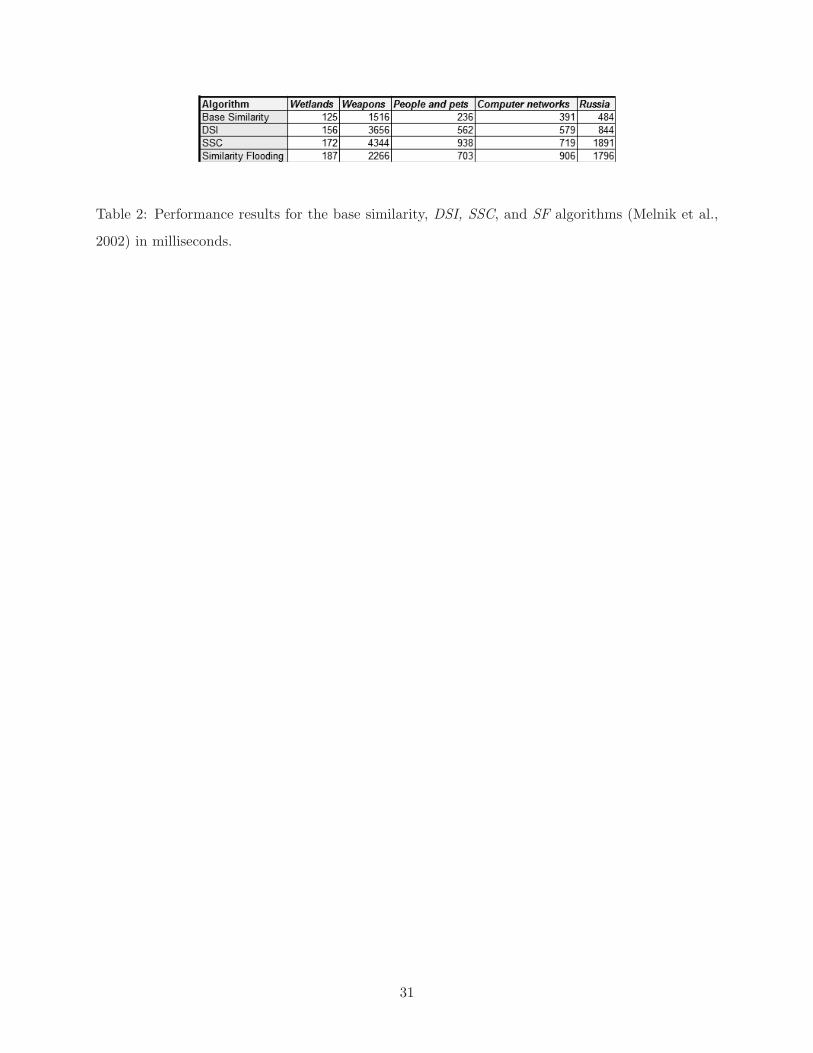
Table 2: Performance results for the base similarity, DSI, SSC, and SF algorithms (Melnik et al.,

2002) in milliseconds.

31

Table 3: Precision and recall for the DSI, SSC, and SF algorithms (wetlands ontology set).

32

Table 4: Precision and recall for the DSI, SSC, and SF algorithms (weapons ontology set).

33

Table 5: Precision and recall for the DSI, SSC, and SF algorithms (people and pets ontology set).

34

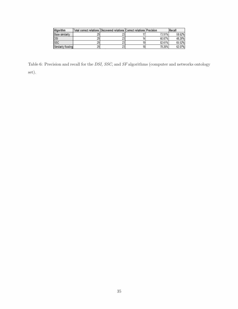
Table 6: Precision and recall for the DSI, SSC, and SF algorithms (computer and networks ontology

set).

35

Table 7: Precision and recall for the DSI, SSC, and SF algorithms (Russia ontology set).

36

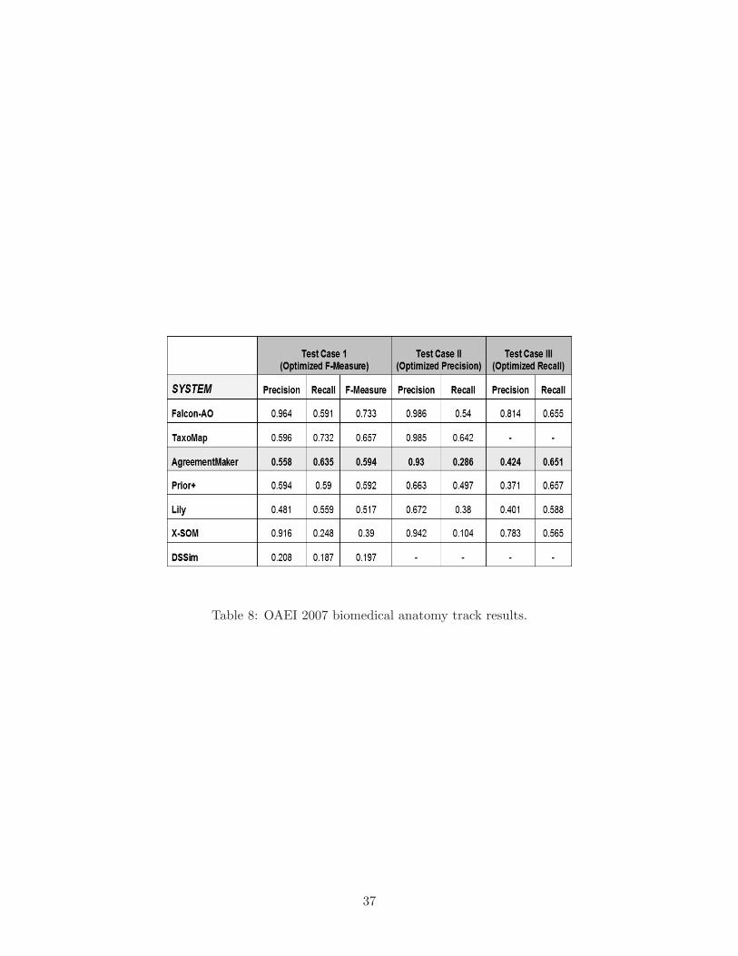
Table 8: OAEI 2007 biomedical anatomy track results.

37

Marine

Estuarine

Lacustrine

Palustrine

Riverine

USAWetland

Classification

Subtidal

Intertidal

Subtidal

Intertidal

Limentic

Littoral

Tidal

LowerPerennial

UpperPerennial

Intermittent

Rock Bottom

Unconsolidated BottomAquatic Bed

Reef

Aquatic BedReef

Rocky Shore

Unconsolidated Shore

Rock Bottom

Unconsolidated Bottom

Aquatic BedReef

Aquatic BedReef

Rocky Shore


Streambed

Emergent Wetland

Scrub-Shrub Wetland

Forested Wetland

Rock Bottom


Aquatic Bed

Rock Bottom


Aquatic BedRocky Shore


Emergent Wetland

Rock BottomUnconsolidated Bottom

Aquatic BedUnconsolidated Shore

Moss-Lichen WetlandEmergent Wetland

Scrub-Shrub Wetland

Forested Wetland

Rock BottomUnconsolidated Bottom

Aquatic Bed

Rocky ShoreUnconsolidated Shore

Emergent Wetland

Streambed

Rock Bottom

Unconsolidated BottomAquatic BedRocky Shore


Emergent Wetland

Rock Bottom

Unconsolidated BottomAquatic BedRocky Shore


Streambed

Figure 1: Cowardin wetland ontology (used in the USA) (Cruz et al., 2005).

38

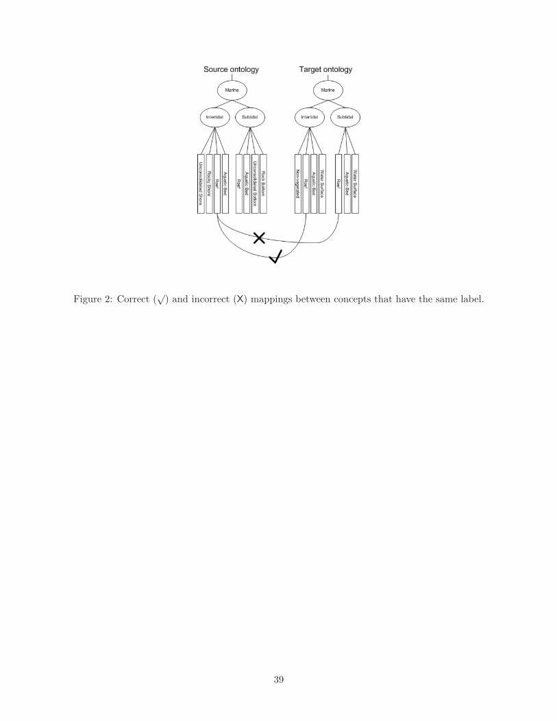
Figure 2: Correct (√

) and incorrect (X) mappings between concepts that have the same label.

39

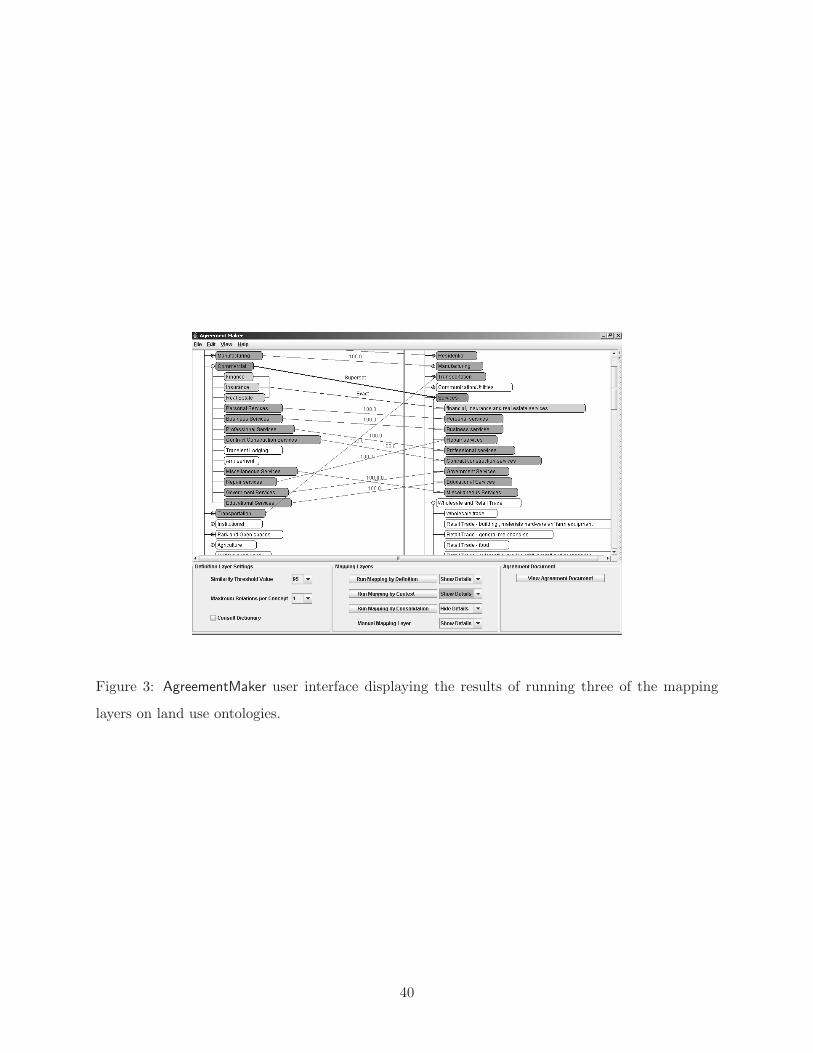
Figure 3: AgreementMaker user interface displaying the results of running three of the mapping

layers on land use ontologies.

40

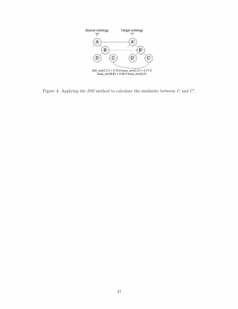
Figure 4: Applying the DSI method to calculate the similarity between C and C ′.

41

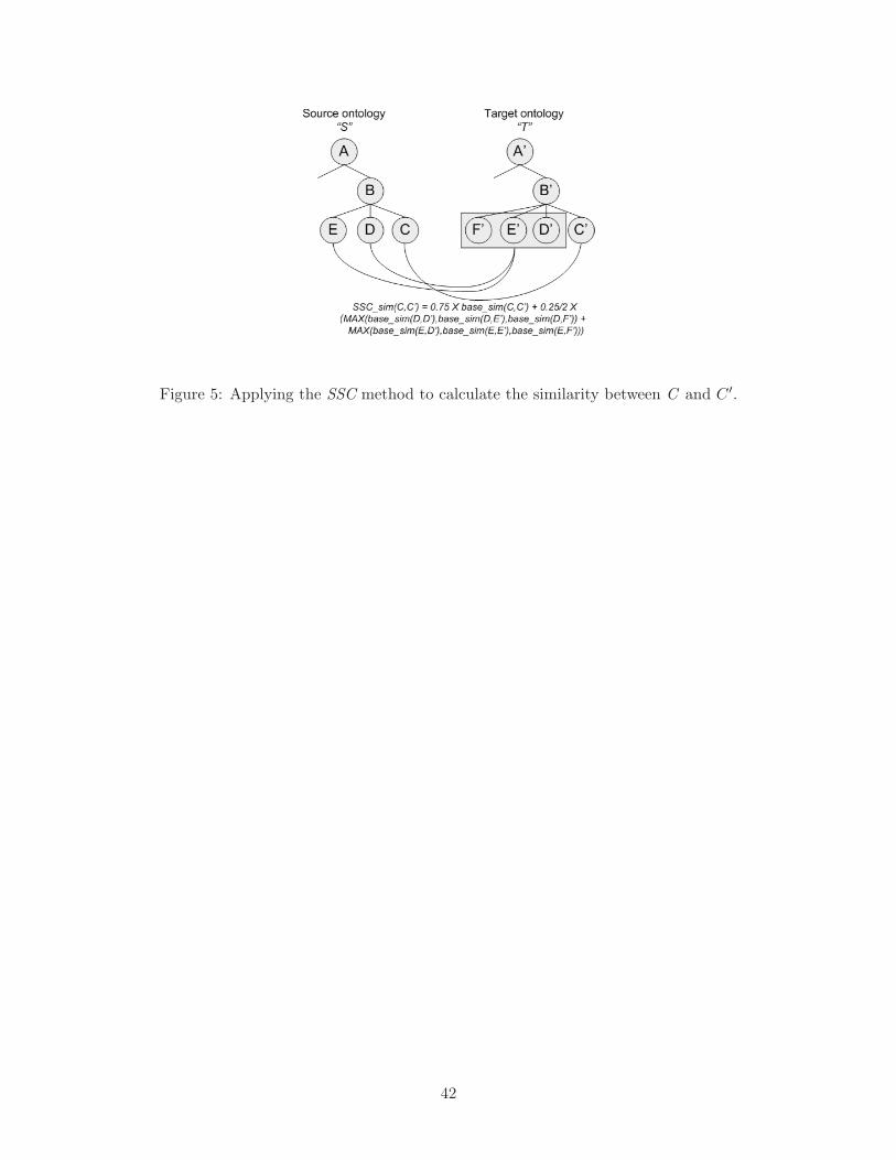
Figure 5: Applying the SSC method to calculate the similarity between C and C ′.

42

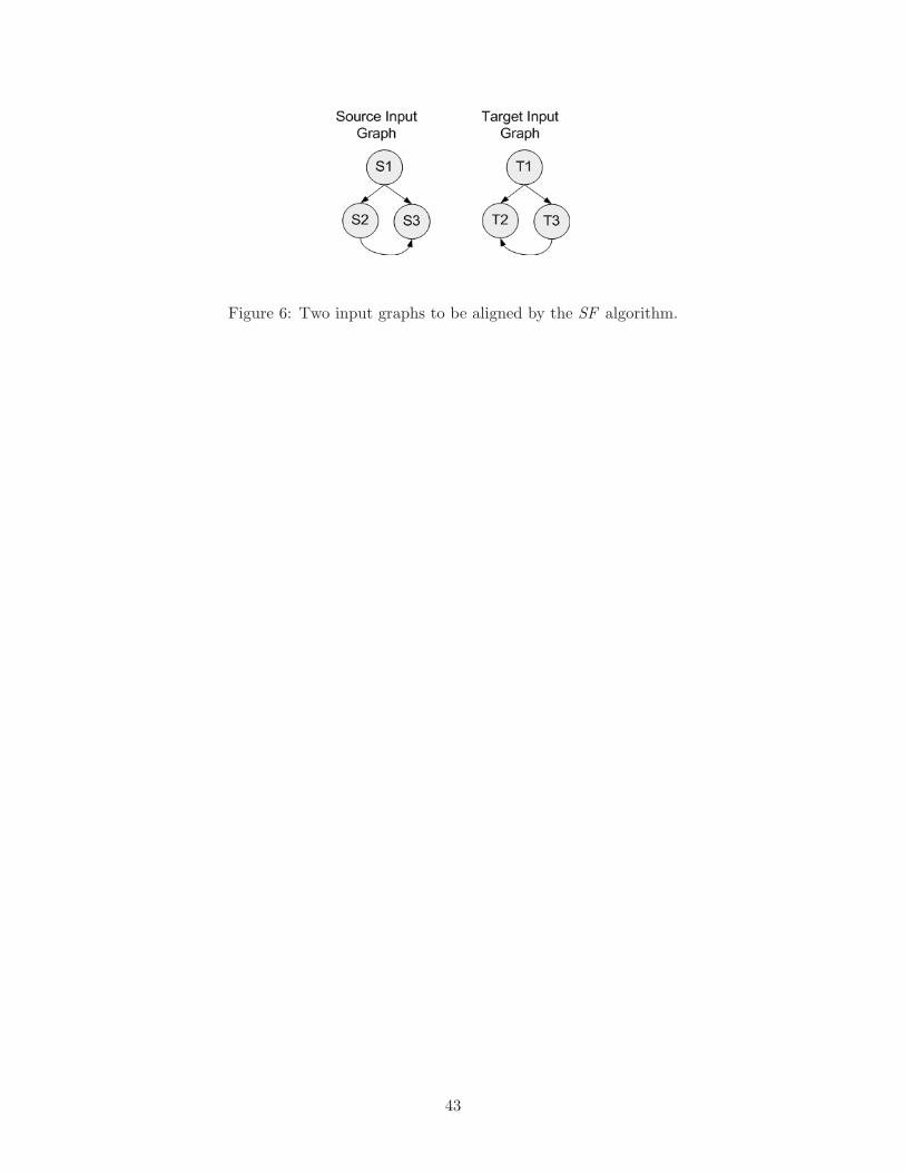
Figure 6: Two input graphs to be aligned by the SF algorithm.

43

Figure 7: Induced propagation graph showing how similarity is propagated between neighbors.

44

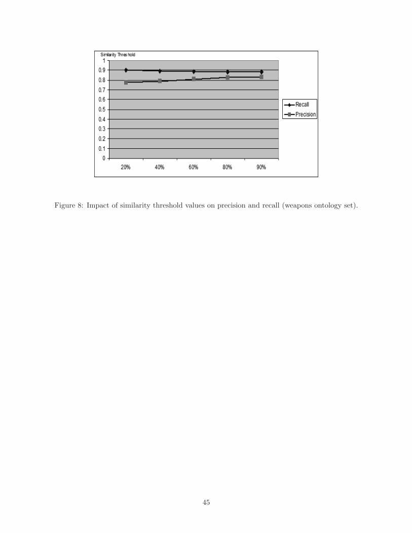
Figure 8: Impact of similarity threshold values on precision and recall (weapons ontology set).

45

Figure 9: Impact of similarity threshold values on precision and recall (people and pets ontology

set).

46

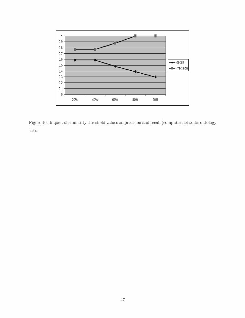
Figure 10: Impact of similarity threshold values on precision and recall (computer networks ontology

set).

47

Figure 11: Impact of similarity threshold values on precision and recall (Russia ontology set).

48

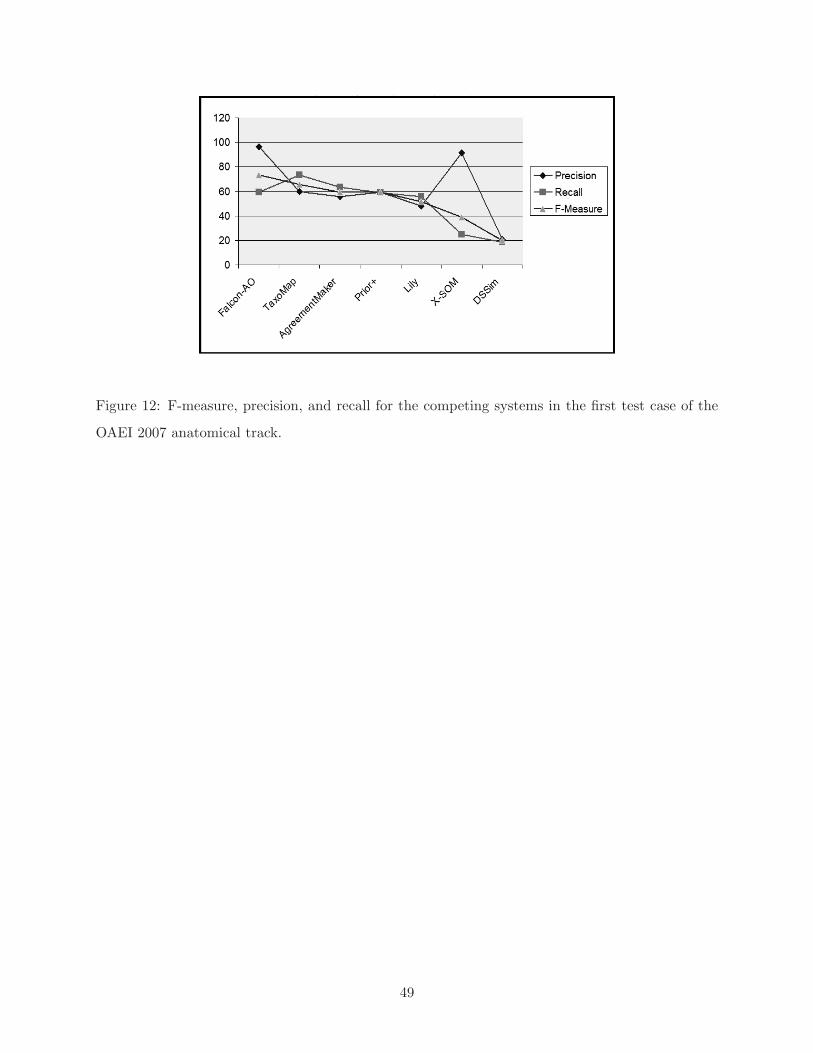
Figure 12: F-measure, precision, and recall for the competing systems in the first test case of the

OAEI 2007 anatomical track.

49

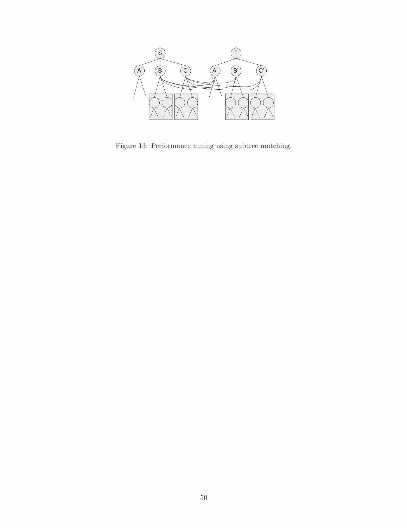
Figure 13: Performance tuning using subtree matching.

50

Figure 14: Runtime before and after performance tuning for the base similarity method for the

four test cases.

51

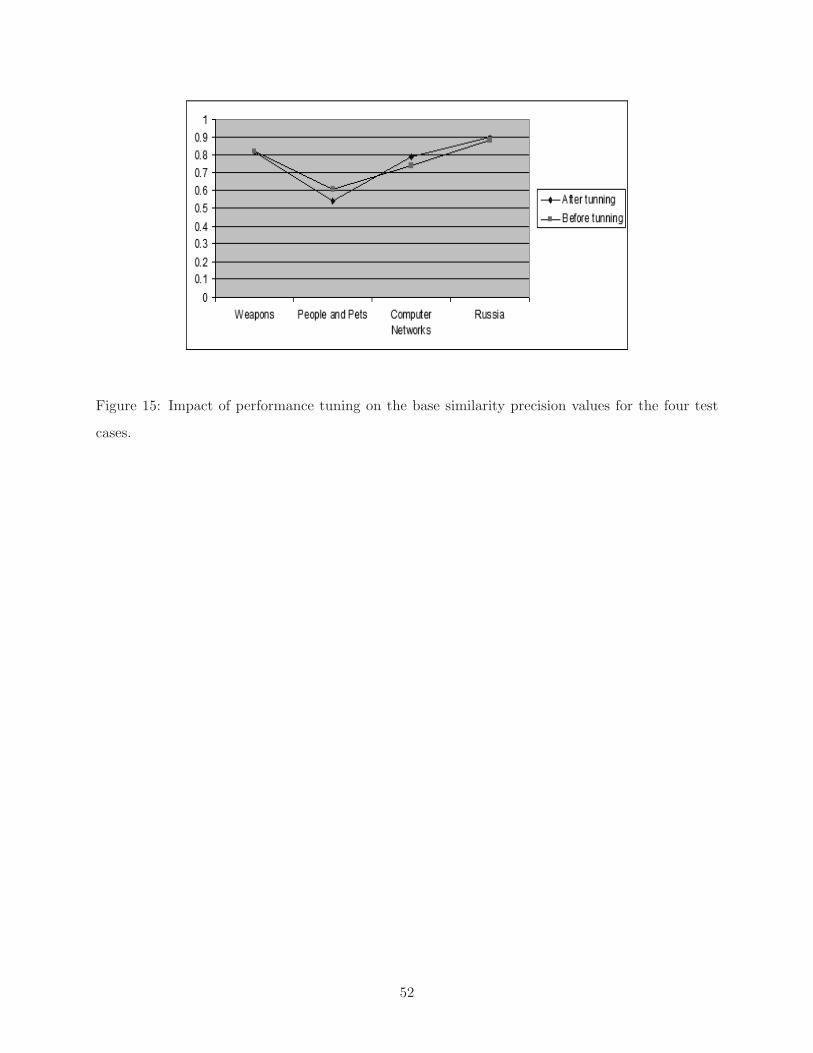
Figure 15: Impact of performance tuning on the base similarity precision values for the four test

cases.

52

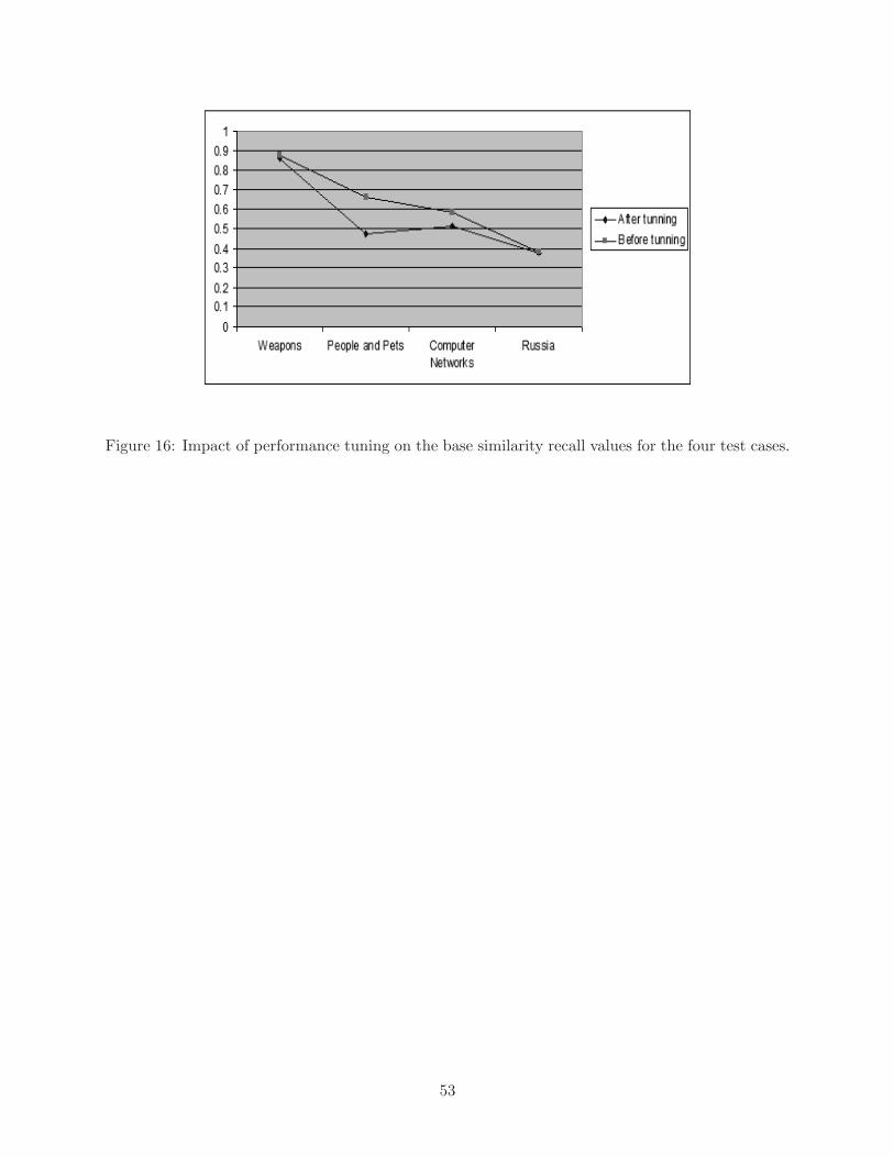
Figure 16: Impact of performance tuning on the base similarity recall values for the four test cases.

53

Figure 17: Runtime before and after performance tuning for the DSI for the four test cases.

54

Figure 18: Impact of performance tuning on the DSI precision values for the four test cases.

55

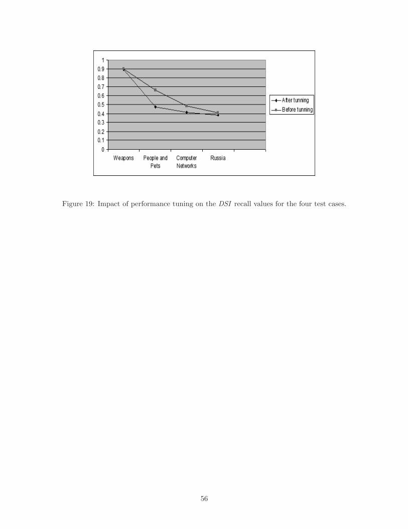
Figure 19: Impact of performance tuning on the DSI recall values for the four test cases.

56

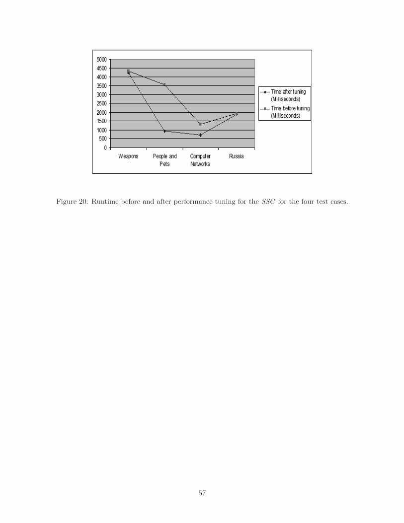
Figure 20: Runtime before and after performance tuning for the SSC for the four test cases.

57

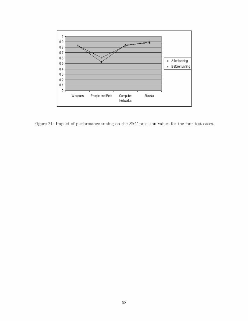
Figure 21: Impact of performance tuning on the SSC precision values for the four test cases.

58

Figure 22: Impact of performance tuning on the SSC recall values for the four test cases.

59

List of Tables

1 Depth and number of concepts in the ontology sets. . . . . . . . . . . . . . . . . . . 30

2 Performance results for the base similarity, DSI, SSC, and SF algorithms (Melnik

et al., 2002) in milliseconds. . . . . . . . . . . . . . . . . . . . . . . . . . . . . . . . . 31

3 Precision and recall for the DSI, SSC, and SF algorithms (wetlands ontology set). . 32

4 Precision and recall for the DSI, SSC, and SF algorithms (weapons ontology set). . . 33

5 Precision and recall for the DSI, SSC, and SF algorithms (people and pets ontology

set). . . . . . . . . . . . . . . . . . . . . . . . . . . . . . . . . . . . . . . . . . . . . . 34

6 Precision and recall for the DSI, SSC, and SF algorithms (computer and networks

ontology set). . . . . . . . . . . . . . . . . . . . . . . . . . . . . . . . . . . . . . . . . 35

7 Precision and recall for the DSI, SSC, and SF algorithms (Russia ontology set). . . . 36

8 OAEI 2007 biomedical anatomy track results. . . . . . . . . . . . . . . . . . . . . . . 37

60

List of Figures

1 Cowardin wetland ontology (used in the USA) (Cruz et al., 2005). . . . . . . . . . . 38

2 Correct (√

) and incorrect (X) mappings between concepts that have the same label. 39

3 AgreementMaker user interface displaying the results of running three of the mapping

layers on land use ontologies. . . . . . . . . . . . . . . . . . . . . . . . . . . . . . . . 40

4 Applying the DSI method to calculate the similarity between C and C ′. . . . . . . . 41

5 Applying the SSC method to calculate the similarity between C and C ′. . . . . . . . 42

6 Two input graphs to be aligned by the SF algorithm. . . . . . . . . . . . . . . . . . 43

7 Induced propagation graph showing how similarity is propagated between neighbors. 44

8 Impact of similarity threshold values on precision and recall (weapons ontology set). 45

9 Impact of similarity threshold values on precision and recall (people and pets ontol-

ogy set). . . . . . . . . . . . . . . . . . . . . . . . . . . . . . . . . . . . . . . . . . . . 46

10 Impact of similarity threshold values on precision and recall (computer networks

ontology set). . . . . . . . . . . . . . . . . . . . . . . . . . . . . . . . . . . . . . . . . 47

11 Impact of similarity threshold values on precision and recall (Russia ontology set). . 48

12 F-measure, precision, and recall for the competing systems in the first test case of

the OAEI 2007 anatomical track. . . . . . . . . . . . . . . . . . . . . . . . . . . . . . 49

13 Performance tuning using subtree matching. . . . . . . . . . . . . . . . . . . . . . . . 50

14 Runtime before and after performance tuning for the base similarity method for the

four test cases. . . . . . . . . . . . . . . . . . . . . . . . . . . . . . . . . . . . . . . . 51

15 Impact of performance tuning on the base similarity precision values for the four test

cases. . . . . . . . . . . . . . . . . . . . . . . . . . . . . . . . . . . . . . . . . . . . . 52

16 Impact of performance tuning on the base similarity recall values for the four test

cases. . . . . . . . . . . . . . . . . . . . . . . . . . . . . . . . . . . . . . . . . . . . . 53

17 Runtime before and after performance tuning for the DSI for the four test cases. . . 54

18 Impact of performance tuning on the DSI precision values for the four test cases. . . 55

19 Impact of performance tuning on the DSI recall values for the four test cases. . . . . 56

20 Runtime before and after performance tuning for the SSC for the four test cases. . . 57

21 Impact of performance tuning on the SSC precision values for the four test cases. . . 58

22 Impact of performance tuning on the SSC recall values for the four test cases. . . . . 59

61

Documents

Structural Alignment Methods with Applications to Geospatial