Stochastic Pricing for Embedded Options in Life Insurance and

© 2008 Society of Actuaries

Stochastic Pricing for Embedded Options in Life Insurance and Annuity Products

Milliman, Inc

October 2008

Tim Hill, FSA, MAAA Dale Visser, FSA, MAAA Ricky Trachtman, ASA, MAAA


Table of Contents

I. Introduction ................................................................................................1

II. Universal Life with Secondary Guarantees: Specifications and

Assumptions...............................................................................................3

III. Variable Annuity Product: Specifications and Assumptions.....................6

IV. Valuing Embedded Options .......................................................................9

V. Generation of Scenarios .............................................................................14

VI. Valuing Annuity Product Embedded Options ...........................................21

VII. Valuing Life Insurance Embedded Options...............................................28

VIII. Attribution Analysis ...................................................................................33

IX. Longitudinal Analysis ................................................................................47

X. Integration into Pricing ..............................................................................53

XI. Comparison to Similar Calculations ..........................................................57

XII. Conclusions ................................................................................................59

XIII. Bibliography...............................................................................................61

Appendices

Appendix A - Universal Life with Secondary Guarantee Specifications and Assumptions..62

Appendix B - Variable Annuity with Guaranteed Lifetime Withdrawal Benefit Specifications and Assumptions ............................................................................................69

Appendix C – Hull-White Stochastic Scenario Generator ....................................................73

Appendix D – Market Consistent Scenario Parameters for VA with GLWB .......................75

Appendix E - Results from VA with GLWB Models............................................................77


Acknowledgement

The authors would like to thank the Society of Actuaries Project Oversight Group who

supported this work with their time and expertise. The POG consisted of:

Bud Ruth, Chair

Claire Bilodeau

Eric Clapprood

Susan Deakins

Steve Largent

Jan Schuh

Ronora Stryker

1


I. Introduction

The genesis of this project was a request from the Society of Actuaries for research

regarding stochastic pricing of embedded options.

In addressing this topic, our approach focuses on two popular insurance products that

have different sensitivities to market conditions. The two products are a variable annuity

(VA) with a guaranteed lifetime withdrawal benefit (GLWB) and a universal life product

with a secondary guarantee (ULSG). Detailed summaries of the specific products are

provided in Sections II and III and associated appendices of this report.

Our research focuses on the challenges associated with market-consistent valuation as

called for by FAS 133. The examination includes the following:

1. Closed-Form Solutions – Can answers be reached using formulas rather than

stochastic analysis?

2. Scenario Generation

a. What models are appropriate for replicating market prices of derivatives?

b. What sources are there for calibrating models?

c. How many scenarios is enough?

3. Liability Assumptions – What dynamic lapse, dynamic utilization and other

assumptions are appropriate?

4. How can results be validated and understood?

2


While our research will touch on topics such as C3 Phase II and III, VACARVM, and

principle-based reserves, our primary focus will be on a “fair value” assessment of

embedded options. The ancillary topics will be addressed in a qualitative rather than

quantitative manner.

Our research goes beyond simply calculating values toward understanding results both on

a point-in-time basis and period-to-period change. It is our opinion that this is where

much of the research is needed. There are numerous groups that calculate the value of

embedded options, but few or none are focusing on understanding and communicating

the results. A key area of our research report explains period-to-period changes in the

value. This is a critical area for the pricing of embedded options because the value itself

is often not as important as the volatility of the value and understanding or even hedging

the volatility.

The final phase of our research uses the results of the prior phases to discuss financial

projections and product pricing. This phase will also discuss the challenges of stochastic-

on-stochastic models and suggests ways to address these challenges.

As the products offered by insurance companies become more and more complex, often

incorporating sophisticated guarantee mechanisms, a method of accounting for the value

of these embedded options becomes more important.

3


II. Universal Life with Secondary Guarantees: Specifications and Assumptions

The universal life with secondary guarantee (ULSG) product specifications and

assumptions were chosen to be representative of the features that are available in the

current marketplace. The product was priced to arrive at an after-tax, after-capital internal

rate of return of 9.0 percent. It is our opinion that this is representative of the pricing

target for ULSG products. Detailed product pricing results are provided.

The secondary guarantee for this product is provided by utilizing a shadow account. The

shadow account parameters vary cell-by-cell to achieve a competitive premium while

maintaining a reasonable profit.

The base UL chassis is typical of what is seen in this market. It will produce cash values,

but they are certainly not the focus of the product. Appendix A contains detailed product

specifications and assumptions.

Table II.2 is a summary of the source of profits for the block of cells under the specifications and

assumptions detailed in the appendix. The margins are defined in Table II.1.:

4


TABLE II.1 – SUMMARY OF MARGIN COMPONENTS

Margin Margin Components

Interest Margin Interest earned on account value and product cash flow less interest credited to the account value

Mortality Margin Account value released on death plus COI charges less death benefits

Surrender Margin Account value released on surrender less surrenders paid

Expense Margin Policy loads less maintenance expenses less acquisition expenses less commissions

AV/Reserve Margin

Change in account value less change in reserve

5


Face Amount:

After-Tax Increase StockINTEREST MORTALITY SURRENDER EXPENSE AV/RESERVE Pre-Tax DAC Other After-Tax Int on in Required Holder

t MARGIN MARGIN MARGIN MARGIN MARGIN Profit Tax FIT Profit Req Capital Capital Divs-- ------------ ------------ ------------ ------------ ------------ ------------ ------------ ------------ ------------ ------------ ------------ ------------1 (299) 569 - (6,236) 1,241 (4,726) 115 (1,654) (3,187) - 641 (3,829) 2 109 799 271 278 (475) 982 93 397 492 26 41 476 3 191 878 436 254 (733) 1,025 74 423 529 28 41 516 4 272 931 479 234 (1,638) 278 56 212 9 29 67 (29) 5 398 977 420 218 (2,430) (418) 41 (79) (380) 32 92 (440) 6 567 1,025 326 205 (2,462) (339) 28 (59) (307) 36 92 (363) 7 736 1,078 227 195 (2,500) (264) 16 (39) (242) 40 95 (297) 8 906 1,129 155 187 (2,598) (221) 6 (25) (202) 43 99 (257) 9 1,081 1,174 93 182 (2,784) (255) (4) (36) (214) 47 106 (273)

10 1,268 1,238 88 176 (2,883) (113) (13) 1 (101) 52 101 (150) 11 1,458 1,277 83 223 (3,364) (323) (16) (82) (225) 56 109 (277) 12 1,668 1,305 70 216 (3,318) (59) (14) (4) (41) 60 98 (79) 13 1,869 1,304 59 209 (3,253) 187 (12) 72 127 64 88 103 14 2,060 1,277 48 201 (3,180) 407 (11) 142 275 68 77 266 15 2,240 1,222 38 193 (3,023) 671 (11) 220 462 71 64 469 16 2,405 1,104 30 186 (2,801) 924 (11) 300 634 74 52 655 17 2,553 947 22 178 (2,580) 1,121 (11) 367 764 76 42 798 18 2,682 614 15 166 (2,093) 1,384 (11) 461 933 77 30 981 19 2,780 66 9 140 (1,435) 1,559 (11) 524 1,046 79 19 1,106 20 2,846 (261) 4 114 (985) 1,718 (11) 579 1,150 79 8 1,222 21 2,885 (692) - (11) (145) 2,037 (12) 692 1,357 80 (9) 1,446 22 2,883 (964) - (47) 37 1,908 (12) 646 1,274 79 (12) 1,365 23 2,876 (1,016) - (46) 164 1,978 (12) 672 1,317 79 (21) 1,418 24 2,856 (1,124) - (45) 350 2,037 (12) 692 1,357 78 (31) 1,466 25 2,824 (1,283) - (43) 573 2,070 (12) 707 1,375 77 (40) 1,491 26 2,777 (1,283) - (41) 693 2,145 (12) 714 1,443 75 (53) 1,571 27 2,716 (1,353) - (39) 799 2,124 (12) 708 1,427 73 (58) 1,558 28 2,650 (1,434) - (37) 930 2,110 (12) 706 1,416 71 (63) 1,550 29 2,569 (1,812) - (51) 1,239 1,946 (12) 652 1,305 68 (64) 1,437 30 2,480 (1,795) - (47) 1,277 1,915 (12) 643 1,284 66 (70) 1,419 31 2,384 (2,053) - (46) 1,590 1,876 (11) 631 1,256 63 (75) 1,394 32 2,272 (2,169) - (53) 1,631 1,680 (11) 564 1,127 60 (73) 1,260 33 2,162 (2,144) - (50) 1,667 1,635 (11) 549 1,097 57 (77) 1,231 34 2,049 (2,139) - (46) 1,701 1,565 (11) 527 1,048 54 (77) 1,179 35 1,937 (1,963) - (42) 1,576 1,509 (10) 506 1,013 50 (78) 1,141 36 1,827 (2,033) - (39) 1,679 1,434 (10) 484 959 47 (78) 1,085 37 1,715 (1,968) - (36) 1,649 1,360 (9) 458 912 44 (77) 1,033 38 1,602 (1,968) - (38) 1,605 1,200 (9) 404 805 41 (73) 919 39 1,495 (1,871) - (35) 1,544 1,134 (9) 381 761 38 (72) 871 40 1,390 (1,868) - (34) 1,545 1,034 (8) 348 693 35 (70) 799 41 1,286 (1,838) - (31) 1,556 973 (8) 327 653 32 (69) 755 42 1,181 (1,832) - (30) 1,552 872 (7) 292 586 29 (66) 681 43 1,081 (1,787) - (27) 1,547 813 (7) 272 548 27 (63) 638 44 981 (1,765) - (28) 1,491 678 (6) 225 459 24 (57) 540 45 888 (1,692) - (28) 1,406 574 (6) 189 390 22 (52) 464 46 802 (1,624) - (25) 1,365 518 (5) 172 351 20 (49) 419 47 722 (1,484) - (23) 1,243 458 (5) 153 310 18 (45) 373 48 647 (1,386) - (20) 1,167 408 (4) 136 276 16 (42) 334 49 578 (1,232) - (18) 1,040 368 (4) 121 250 14 (39) 303 50 514 (1,192) - (16) 1,033 339 (3) 113 229 13 (37) 279 51 452 (1,093) - (14) 955 300 (3) 101 202 11 (34) 248 52 396 (992) - (13) 875 265 (3) 88 180 10 (31) 221 53 344 (906) - (11) 805 232 (2) 77 158 9 (29) 195 54 297 (788) - (10) 698 198 (2) 65 135 7 (25) 167 55 256 (699) - (8) 621 170 (2) 56 115 6 (22) 144 56 220 (621) - (7) 565 157 (2) 52 106 6 (20) 131 57 187 (529) - (6) 476 127 (1) 41 87 5 (17) 109 58 159 (491) - (5) 444 107 (1) 36 73 4 (15) 92 59 133 (425) - (5) 385 89 (1) 30 60 3 (14) 77 60 111 (365) - (4) 330 73 (1) 24 50 3 (12) 64 61 92 (317) - (3) 288 60 (1) 19 41 2 (10) 54 62 75 (279) - (3) 256 50 (1) 17 34 2 (9) 45 63 61 (223) - (2) 205 41 (1) 13 28 2 (8) 37 64 49 (202) - (2) 184 29 (1) 10 20 1 (6) 28 65 39 (154) - (1) 147 30 (0) 10 21 1 (5) 27 66 30 (137) - (1) 143 35 (0) 12 24 1 (5) 29 67 23 (96) - (1) 93 18 (0) 6 13 1 (3) 17 68 17 (84) - (1) 81 13 (0) 4 9 0 (3) 12 69 13 (64) - (1) 62 10 (0) 3 7 0 (2) 9 70 9 (49) - (0) 48 7 (0) 2 5 0 (2) 7 71 7 (40) - (0) 38 5 (0) 2 3 0 (1) 5 72 5 (29) - (0) 27 3 (0) 1 2 0 (1) 3 73 3 (20) - (0) 20 3 (0) 1 2 0 (1) 3 74 2 (15) - (0) 15 2 (0) 1 2 0 (1) 2 75 1 (10) - (0) 10 2 (0) 0 1 0 (0) 1 76 1 (7) - (0) 18 12 (0) 4 8 0 (1) 8

Present Value of Margins, discounted at 8.0%

15,174 5,645 1,860 (4,005) (16,093) 2,582 273 1,207 1,101 569 1,121 550

Table II.2: ULSG - Source of Profits

$250,000

6


III. Variable Annuity Product: Specifications and Assumptions

The variable annuity (VA) product specifications and assumptions used in this report

were chosen because they are representative of the features available in the current

marketplace. The mortality and expense (M&E) charge was solved for to arrive at an

after-tax, after-capital return on assets (ROA) of around 20 basis points. The ROA was

calculated by discounting the statutory after-tax, after-capital earnings at 8 percent and

dividing by the present value of the average annual account value. A breakdown of the

sources of profit is provided.

The guaranteed minimum death benefit (GMDB) chosen for this model is a simple return

of premium design. This was chosen so that the focus of the analysis remains on the

guaranteed living benefit. The cost of the GMDB was assumed to be in the 10 basis-point

range and has been added to the M&E charge at cost.

The guaranteed lifetime withdrawal benefit (GLWB) specifications were chosen because

they are representative of the types of benefits seen in the marketplace. The charge for the

GLWB, 65 basis points of account value, was set to be typical in the marketplace, with

coverage of the hedge cost and a modest additional margin for capital and reserves plus

volatility in the hedge cost.

Appendix B contains the detailed product specifications and assumptions.

The following Table III.1 is a sources of profit report that outlines the effects that each

element of the profits for this product has over the total profitability of the product. The

revenue area is composed of investment income on reserves and cash, M&E charges, the

withdrawal margin (surrender charges), and revenue sharing. The expense area is

composed of death benefits (excess of the amount of death benefits above the account

value released at time of death), acquisition expenses, maintenance expenses and

7


commission. The timing difference of the release in reserves is accounted for by the

difference in the change of account value by the change in reserves. The pre-tax profit is

obtained by subtracting from the total revenue the total expenses and then adding the

reserve allowance. Taxes are subtracted to obtain the after-tax profit and required capital

is taken into account to obtain the adjusted after-tax statutory profits. Each of the

elements is discounted back to time zero and divided by the average account value in

force to obtain a sources of profit report that measures the return on account value

(ROA).

8


Table III.1 - Base VA Product - Sources of Profit VA Embedded Options--Proj.001--Base VA

SOURCES OF PROFITS Projection Module Summary Page 1 Description: Sources of Profit (bps) SOA Research Project Projection Mode: Annual 9/17/2007 10:25:14 AMProjection Date: 12/2006 MG-ALFA 6.4.238 / 931RDO03-59_VA_09-17-

07 Projection Cycles: 30 (Annual) ROA in bps of AV Capital Strain

Investment Income -14.28 PV Yr 1 Profit/ PV Premium -1.82%M&E Charges 99.36 Withdrawal Margin 9.05 PV of Profit 847.88Revenue Sharing 36.13 PV Premium 50,000

Total Revenue 130.26 PV of Profit/ PV Premium 1.70%

DB Benefits 0.00 GIRR 18.30%Acq Exp 20.38 Main Exp 12.44 PV of Profit/ PV of Avg AV 0.21%Net Commission 80.96

Total Expense -113.78

Change In AV 695.40 Change In Reserves -671.29

Total Chg 24.12 Total Profit 40.60

Taxes -15.29 Total After-Tax Profit 25.31

Interest on TS 2.73 Change in TS -6.71

Capital -3.99 Total Adjusted Profit 21.33

9


IV. Valuing Embedded Options

A life insurance contract or an annuity can contain many embedded options. Some of

those embedded options, such as minimum interest rates, are fairly explicit while others,

such as guaranteed face amount increase options and the mortality aspects of guaranteed

annuitization options, are less obvious. Historically, many of these options were included

in the contract without explicitly being priced. Many of the options were thought to be

conservatively designed and would rarely, if ever, come into play. However, the recent

low interest rate period has certainly proven that theory wrong.

As competitive pressures in the insurance industry have continued to increase, including

stronger guarantees (more favorable to the policyholder) in product offerings have been

one way for companies to distinguish their products from those of their competitors. The

two products that are the focus of this research project have certainly experienced this

company practice.

The variable annuity market is largely dominated by various types of guarantees.

Guaranteed minimum death benefits appeared on variable annuities approximately 15

years ago. Living benefits have been offered on variable annuities for just over 10 years.

Today, guaranteed minimum income benefits (GMIB), guaranteed minimum withdrawal

benefits (GMWB), guaranteed lifetime withdrawal benefits (GLWB), and guaranteed

minimum accumulation benefits (GMAB) are significant drivers of variable annuity

sales. In fact, a guaranteed living benefit (GLB) is offered as a rider on at least 90 percent

of variable annuity sales and the GLB is elected in over 70 percent of sales1.

The simplest form of the GLB is the GMAB. The benefit closely resembles a put option.

The typical structure might be a return of premium guarantee after a 10-year waiting

period. If the account value is less than the GMAB value (the premium in this example),

1 2007 Milliman Guaranteed Living Benefit Survey

10


the account value will be “topped-off” to equal the GMAB. Therefore, the benefit is

simply equal to the following:

Max (0, GMAB – AV) of the 10th anniversary

This benefit is identical to a 10-year put option except for the following:

1. The GMAB is dependent on the survival of the annuitant and the persistency of

the base contract, while a put option is a free-standing contract.

2. The account value of the VA has fees that reduce the performance. Typical fees

might include 120 bps M&E, 100 bps fund management fees, and 50 bps for the

GMAB versus an S&P 500 index.

3. The charge for the GMAB is typically assessed against the account value or

benefit base versus an upfront premium for the put option.

Because of the relative simplicity of the GMAB, the value of the embedded option

provided by the GMAB can be approximated by a Black-Scholes formula. The inputs

into the formula and the formula itself are as follows.

Risk-free rate = 5.0% Total fees = 270 bps Assumed volatility = 17.0% Duration = 10 years Strike price = $1,000 Premium = $1,000 10th Anniversary Persistency = 50% Let St = Current price of the fund m = Margin deducted from the policyholder fund Smt = St*(1-m)T-t = Starting Account Value adjusted for regular charges deducted from it K = Exercise price or Strike price r = Risk-free rate

11


T = maturity t = current duration BSP = Black-Scholes European Put Option = )()( 12

)( dSmdKe ttTr −Φ−−Φ−−

where:

σ

σ

tT

rtTK

Sm

d

t

−

+−+⎟⎠⎞

⎜⎝⎛

=)

2)((log

2

1

tTdd −−= σ12

GMAB = BSP * Persistency

Table IV.1 below contains an example of GMAB embedded option prices using the

Black-Scholes formula and the above inputs.

Table IV.1 - Example of GMAB Embedded

Option Prices as a Percent of GMAB Strike Price Time At-the-

money Out-of-the-money 20%

In-the-money 20%

0 4.01% 2.52% 6.39% 5 4.16% 2.12% 7.82%

So, a closed-form equation like the Black-Scholes formula can be used to value the

embedded option for a GMAB. However, a more complicated benefit like a GLWB

requires a stochastic method. A GLWB has a stream of benefits, not just a single

payment. A GLWB also provides flexible benefits, where the customer may decide when

partial withdrawals start and stop.

A GLWB guarantees a stream of partial withdrawals for the annuitant’s life, regardless of

the account value. For instance, given a $100,000 premium, a 5 percent for life GLWB

would guarantee partial withdrawals of $5,000 per year for the life of the annuitant. In a

poor investment return scenario, the account value may eventually go to zero. When this

happens, the insurance company will typically issue a single premium immediate annuity

12


for the remaining payments for the life of the annuitant. The present value of the SPIA at

the moment the account value goes to zero is the embedded option that will be captured

for the GLWB.

A detailed example of this calculation is provided in Section VI.

Largely in response to the low interest rate environment and the reserve pressure

associated with long duration term insurance products, the life insurance industry began

to offer more and more generous no-lapse guarantees on universal life contracts. These

no-lapse guarantees are often called secondary guarantees. The product category in

general is often referred to as universal life with secondary guarantees (ULSG). They

guarantee that as long as a specific criterion is met, the contract will not lapse, even if the

cash value goes to zero. Without the no-lapse guarantee, the traditional universal life

contract would lapse once the cash value reaches zero. This could happen during a period

of low interest rates, where the credited interest and premiums paid are not sufficient to

cover the contract charges (e.g., cost-of-insurance, other loads, etc.).

No-lapse guarantees are generally structured in one of two ways, although the distinction

is blurred. Originally, these guarantees were based on the cumulative premiums paid,

exceeding a specified annual amount times the number of years that had passed. This

type of criteria is a “specified premium” design. As this design evolved, interest credits

(e.g., 5 percent) were applied to excess premiums that were paid and the specified annual

amount may no longer be a constant amount (typically increasing if not level).

The other no-lapse guarantee structure involves the use of a second account value-type

calculation, often called a shadow account. The shadow account typically functions much

like the account value, except that all of the parameters are guaranteed, including the

interest rate. The fact that all values are guaranteed allows the customer to see exactly

how long the contract will remain in force. It also allows the customer and agent to solve

13


for the premiums necessary to keep the contract in force until maturity (lifetime

guarantee).

For the purposes of this research report, we chose a shadow account design, because this

is generally the method used for more competitive products. Actually, the structure,

shadow account versus specified premium, to determine the guarantee really does not

matter for our purposes. The length of the guarantee provided by the specific premium

paid is the only item needed for our research. We chose to use a lifetime guarantee

because this is the most frequent guarantee period used in the industry for these products.

The length of the guarantee is the only item that matters in this exercise, because the

research project measures the amount of death benefits paid, which would not have been

paid without the no-lapse guarantee. This is defined as death benefits paid minus

premiums paid once the cash value has gone to zero. If no additional premiums need to

be paid to keep the no-lapse guarantee in effect, this collapses to just the death benefits

paid once the cash value has gone to zero.

A detailed example of this calculation is provided in Section VII.

14


V. Generation of Scenarios

When the embedded option is determined on a stochastic basis, a key determinant of the

value of the embedded option is the stochastic scenarios used. There are many choices

that can be used to calibrate and generate scenarios. Table V.1 below is a sample of the

categories that scenarios can fall under:

TABLE V.1: SAMPLE CATEGORIES OF SCENARIOS

Category Interest Rates Equity Returns Historic (realistic, probabilistic)

Interest rate scenarios start at the current interest rate curve and reflect historic volatility. There may be a reversion to a mean component. There may be restrictions or requirements for a number of inverted yield-curve occurrences. C3 Phase I or II scenarios would fit this category.

Equity returns are based on historic returns and volatility. Returns might be based on excess over a risk-free rate or might be based purely on average historic returns. Consideration should be made for “fatter” tails than are generally seen with lognormal distributions. Historic correlations should be reflected. C3 Phase II scenarios would fit this category.

Long-Term Risk Neutral

Similar to market consistent but using a smoothed current interest rate curve based on a period of a few years and potentially a “normal” shape.

Similar to market consistent, but with a longer term view of the mean rate and volatility. May use a historic value for both, possibly with some additional conservatism.

Market Consistent

Generally arbitrage free interest rate scenarios where the forward rates are driven by the current yield curve. Interest rate volatility assumptions are being gathered from market instruments such as Swaptions and other interest rate derivatives. The scenarios should be able to replicate derivatives found in the marketplace.

Categorized as risk neutral. Mean returns are based on the current swap curve. Volatility assumptions are based on a term structure of volatility, which needs to be gathered from instruments in the marketplace such as long-dated calls and puts. Beyond the period where instruments are available (generally after five to 10 years), volatilities may remain at the last observed value or may grade back to a historic level. Scenarios should be able to replicate derivative prices found in the market.

15


Each of the scenarios will result in materially different results for the embedded value

calculation. The distinction between the long-term risk neutral and the market consistent

scenarios is the frequency of adjusting the parameters. The long-term risk neutral

scenario set described above relies on a longer term view of market parameters.

Conceptually, this type of a scenario set can be appropriate for a pricing exercise where it

may not be possible to adjust the price on a frequent basis, thereby facilitating a price that

will be appropriate in a variety of market conditions. Market consistent scenarios are

appropriate for calculating current hedge costs, for calculating derivative prices, for

market value calculations like FAS 133 and for any situation where the value needs to be

consistent with other instruments available in the market.

For historic scenarios, we used the scenarios generated for C3 Phase II. Scenarios can be

downloaded from the American Academy of Actuaries (AAA) Web site. Table V.2

below shows the indices used in our model, and the C3 Phase II dataset used for each of

the indices.

TABLE V.2: INDICES USED IN MODEL

Model Index C3 Phase II Dataset

S&P 500 US

Russell 2000 SMALL

NASDAQ AGGR

SB BIG LTCORP

EAFE INTL

Money Market MONEY

For long-term risk neutral scenarios, a lognormal scenario generator was used. The

assumptions used to populate the generator were chosen to include a modest degree of

16


conservatism over historically accurate parameters. The mean return was chosen as a

conservative estimate of the forward rates that would be generated by a typical swap

curve. The volatility rates are 10-year average realized market volatilities increased by

100 to 200 basis points for conservatism. Table V.3 below shows the assumptions:

TABLE V.3 - LONG-TERM RISK NEUTRAL SCENARIO

PARAMETERS

Model Index Mean Return Volatility

S&P 500 5.0% 19.0%

Russell 2000 5.0% 21.5%

NASDAQ 5.0% 28.0%

SB BIG 5.0% 5.0%

EAFE 5.0% 19.5%

Money Market 5.0% 1.0%

1-yr Treasury 4.9% 6.1%



Also, for the long-term risk neutral scenarios, the following correlation matrix, Table

V.4, applies. The correlation matrix is based on a 10-year history.

17


Table V.4 - Long-Term Risk Neutral Scenarios – Correlation Matrix

S&P500 Russell 2000 NASDAQ SBBIG EAFE Money

Market

S&P 500 1.000 .806 .833 -.095 .687 .005

Russell 2000 .806 1.000 .851 -.135 .631 -.025

NASDAQ .833 .851 1.000 -.130 .588 -.019

SBBIG -.095 -.135 -.130 1.000 -.136 .035

EAFE .687 .631 .588 -.136 1.000 -.034

Money Market .005 -.025 -.019 .035 -.034 1.000

For the market consistent scenarios, separate sets were used for the ULSG product and

the VA product. The ULSG product used a set of arbitrage free interest rates based on the

9/30/2007 yield curve. These scenarios were generated using a Hull-White scenario

generator. Appendix C contains a summary of the Hull-White scenario generator.

For the VA product, a lognormal model was used with the parameters summarized in

Charts V.1 and V.2 and Table V.5. The values in Charts V.1 and V.2 can be found in

Appendix D.

18


Chart V.1 - Swap Curve and Resulting Forward Rates

4.8%

5.0%

5.2%

5.4%

5.6%

5.8%

6.0%

6.2%

1 2 3 4 5 6 7 8 9 10 11 12 13 14 15 16 17 18 19 20 25 30

Duration

Inte

rest

Rat

e

9/30/07 Swap Curve

Forward 1-Yr Rates

Chart V.2 - Implied Volatility Term-Structures

0%

5%

10%

15%

20%

25%

30%

35%

40%

1 2 3 4 5 6 7 8 9 10 11 12 13 14 15 16 17 18 19 20

Duration

Vola

tility

S&P Russell 2000

NASDAQ SB BIG

EAFE Money Market

19


The volatility surface was determined using implied volatility data for the first 15 years

and then grading to the historic average over the next five years. Implied volatility data

was derived from market prices on available put options as of 9/30/07. Implied volatility

term structures were then used to create the forward one-year volatilities.

Table V.5 – Correlation Matrix S&P500 Russell

2000 NASDAQ SBBIG EAFE Money

Market S&P 500 1.000 .806 .833 -.095 .687 .005

Russell 2000

.806 1.000 .851 -.135 .631 -.025

NASDAQ .833 .851 1.000 -.130 .588 -.019

SBBIG -.095 -.135 -.130 1.000 -.136 .035

EAFE .687 .631 .588 -.136 1.000 -.034

Money Market

.005 -.025 -.019 .035 -.034 1.000

A key for confirming that the market consistent scenarios are in fact market consistent is

to test whether the price of options available in the marketplace can be reproduced. This

was done for the ULSG scenarios by capturing a 9/30/07 swaption quote. The implied

volatility embedded in the observable price of an at-the-money swaption with a seven-

year tenor and one-year option term on 9/30/07 was 18.6 percent. Our scenarios resulted

in a comparable value of 18.4 percent. The implied volatility embedded in the observable

price of an at-the-money swaption with a 10-year tenor and one-year option term on

9/30/07 was 17.2 percent. Our scenarios resulted in a comparable value of 17.8 percent.

For the VA scenarios, a long dated at-the-money put option is used to confirm the

validity of the scenarios. On 9/30/2007, the market observable price for a 10-year, at-the-

money, S&P 500 put was 7.26 percent. The scenarios were run through an Excel model

20


to calculate the cost of the 10-year put over the 1,000 scenarios. A sample for a single

scenario is shown below in Table V.6.

Table V.6 – Sample Calculation for Single Scenario S&P Index at time 0 (Index0) 1,000.00 S&P Index at time 10 (Index10) 986.25 Strike Price (at-the-money) 1,000.00 Value of Put Option (Max[Strike - Index10,0]) 13.75 Present Value Factor (Continuous Risk Free Rate) 0.56992 Present Value Of Put Option 7.84

The average cost of the put option over the 1,000 scenarios was 7.10 percent.

21


VI. Valuing Annuity Product Embedded Options

Recall that the embedded option being valued for the GLWB is a stream of partial

withdrawals for the annuitant’s life, regardless of the account value. If/when the account

value goes to zero, a single premium immediate annuity is issued to cover the remaining

payments for the life of the annuitant. The present value of the SPIA at the moment the

account value goes to zero is the embedded option that will be captured for the GLWB.

Table VI.1 below is an example of this calculation for a specific scenario:

Table VI.1 – VA Embedded Options Detail VA Embedded Options--Proj.002--GLWB Hedge Cost

Liability Audit, Scenario 2500: 025_--[002--* 065****A1****] Cash Mode: Annual SOA Research Project LOB & Characteristics: VarAnn XM MN 1S 2Y 3A 41 11/19/2007 9:50:08 AMPlan: GLWB-VA MG-ALFA 6.4.279 / TEMP.P05 / 931RDO03-59_VA_09-17-07 Issue Age: 65 Deferral Period 10 Years

Year Month

Beginning Month

Acct Val

GLWB Benefit Base

Maximum Annual GLWB

Partial Withdrawal

Year-To-Date

Cumulative GLWB

Withdrawal Amount

GLWB Excess Over Acct Val

Beginning of Month

Persistency GLWB Credit

1 1 50,000 50,204 2,510 0 0 0 1 5 12 29,972 63,814 3,829 0 0 0 0.858894

10 12 50,936 81,445 4,887 0 0 0 0.358988 15 12 34,368 81,445 4,887 4,887 24,433 0 0.182364 20 12 14,379 81,445 4,887 4,887 48,867 0 0.095504 21 12 7,035 81,445 4,887 4,887 53,754 0 0.088276 22 12 2,231 81,445 4,887 4,887 58,640 0 0.081226 23 4 757 81,445 4,887 1,629 60,269 0 0.078356 23 5 366 81,445 4,887 2,036 60,676 42 0.077275 3.2123 6 0 81,445 4,887 30,241 88,881 28,204 0.076806 2,166.27

PV of GLWB Credit @ 5% = 672.69

The example shows that the account value (AV) runs out 23 years and five months into

the scenario. In fact, the partial withdrawal in 23rd year and fifth month is $366 of account

value and $42 of GLWB value. At that point, the guaranteed benefit stream of $4,887 per

year is discounted back to the date the account value went to zero with 5 percent interest

22


and the assumed mortality table. This equals $28,204 on an undecremented basis and

$2,166.27 on a decremented basis. Discounting the $2,166.27, plus the $3.21, which is

the decremented $42 payment top-off, back to time zero at a 5-percent interest rate gives

$672.69.

The above calculation relies on the portion of policies in force as of the date the AV goes

to zero as part of the calculation. This portion is determined by the mortality assumptions

and the lapse assumption. The lapse assumption used in the example has a dynamic

component that reflects the amount the GLWB is in-the-money. The details of the

formula used are presented in Appendix B.

A typical dynamic lapse formula used in pricing VA guarantees decreases lapses as the

value of the guarantee, the GMWB in this case as measured by the present value of the

guaranteed income stream, increases relative to the account value. The theory is that

customers will be more likely to persist to realize the value of the guarantee than they

would be without the guarantee. The impact of this assumption can be substantial. For

instance, for a 65 year old who waits 10 years to start taking withdrawals and assuming

100 percent aggressive growth asset allocation under market consistent scenarios, the PV

of GLWB credit is $1,800. The same PV of GLWB without the dynamic lapse multiplier

is $1,037. That is a 42-percent decrease in this liability, due to the dynamic lapse

assumption.

Recall that a number of different scenario sets and the times when each was appropriate

were discussed. The difference between the market consistent, long-term risk neutral, and

historic scenarios is often quite large, as shown by the Tables VI.2, VI.3 and VI.4. All

three of these tables assume 100 percent of the VA account value is allocated to the

aggressive growth asset allocation.

23


TABLE VI.2 – PV OF GLWB WITH AGGRESSIVE GROWTH ASSET ALLOCATION

MARKET CONSISTENT SCENARIOS Deferral Period

Issue Age 0 5 10

55 $2,897 $2,259

65 $1,511 $2,717 $1,800

75 $1,126 $1,607 $816

85 $512

Deferral period in Table VI.2, and subsequent tables, is the number of years before the

first withdrawal is taken. Recall that our GLWB product accumulates premiums at 5

percent until the earlier of the 10th anniversary or the first withdrawal. The 10-year

deferral will maximize the value of the benefit base. However, deferring withdrawals

does not necessarily maximize the PV of the GLWB. For instance, note that the PV of

GLWB is $2,717 for issue age 65, five-year deferral and $1,800 for issue age 65, 10-year

deferral. Recall that the payout percent is based on the attained age and would be 6

percent for both the five-year and 10-year deferrals. Even though the benefit base is

higher for the 10-year deferral, starting withdrawals younger, 70 for the five-year deferral

versus 75 for the 10-year deferral, has a larger impact on the PV of GLWB.

In Table VI.3 below, the long-term risk neutral scenario set is used instead of the market

consistent scenarios.

24



LONG-TERM RISK NEUTRAL SCENARIOS Deferral Period

Issue Age 0 5 10

55 $2,776 $2,113

65 $1,437 $2,609 $1,649

75 $1,096 $1,518 $716

85 $503

The values in Table VI.3 are slightly lower than the values in Table VI.2. This is due to

the relationship between the long-term risk neutral parameters and the market consistent

parameters as of 9/30/07.

In Table VI.4 below, the historic scenario set is used instead of the market consistent

scenarios.


HISTORIC SCENARIOS Deferral Period

Issue Age 0 5 10

55 $490 $297

65 $236 $567 $280

75 $230 $366 $126

85 $113

25


Not surprisingly, the values in Table VI.4 are considerably lower than the values in Table

VI.2 or Table VI.3. This is due to the higher mean return associated with equity

subaccounts within the VA.

Another interesting comparison is the impact of the three assumed asset allocations.

Focusing back on Table VI.2 for a moment, if we move from the aggressive growth asset

allocation (approximately 75 percent equity / 25 percent bond) to the moderate aggressive

growth asset allocation (approximately 65 percent equity, 35 percent bond), as shown in

Table VI.5 below, we see a marked reduction in the PV of GLWB.

TABLE VI.5 – PV OF GLWB WITH MODERATE AGGRESSIVE GROWTH ASSET ALLOCATION


Issue Age 0 5 10

55 $2,257 $1,751

65 $1,125 $2,162 $1,400

75 $861 $1,266 $626

85 $388

As the asset allocation is now changed to the moderate growth asset allocation

(approximately 50 percent equity, 50 percent bond) another significant drop in the PV of

GLWB is seen as shown in Table VI.6 below.

26


TABLE VI.6 – PV OF GLWB WITH MODERATE GROWTH ASSET ALLOCATION


Issue Age 0 5 10

55 $1,396 $1,068

65 $633 $1,391 $873

75 $512 $810 $381

85 $234

Focusing on a specific cell for a moment, Issue Age 65 with 10 year deferral, the values

are $1,800 for the aggressive growth asset allocation, $1,400 for the moderate aggressive

growth asset allocation and $873 for moderate growth asset allocation, a reduction of

51.5 percent from the highest to the lowest. Recall that in the market consistent scenarios,

we assume that all subaccounts have the same mean growth rate dictated by the swap

curve. However, as the allocation is moved more toward the bond and money market

subaccounts, the overall volatility of the underlying account value is reduced. This is why

the PV of GLWB is cut in half, going from the aggressive growth asset allocation to the

moderate growth asset allocation.

Now, in looking at the issue age 65 and 10-year deferral period cell using the historic

scenarios, the values are $280 for the aggressive growth asset allocation, $248 (value can

be found in Appendix E) for the moderate aggressive growth asset allocation and $213

for the moderate growth asset allocation, a reduction of 23.9 percent from the highest to

the lowest. This is a significantly lower reduction going from the aggressive growth asset

allocation to the moderate growth asset allocation. In the historic scenarios, a significant

reduction in overall volatility of the underlying account value would again be expected.

However, in the historic scenarios, there is also a corresponding reduction in the mean

27


return expectation as the asset allocation is moved from aggressive growth to moderate

growth, thus the lower percent reduction in PV of GLWB.

The tables above presented the average PV of the GLWB benefits across 1,000 trials.

This prompts the question of how many scenarios are enough. The answer to this

question is not always an easy one. It depends on what types of measures are being

examined and the underlying distribution. For instance, the focus here is on the average

of all the scenarios. It will generally take fewer scenarios to arrive at a high degree of

confidence in the result for an average rather than a 95th or 99th percentile. Percentiles are

highly dependent on only the tail of the distribution, rather than dependency spread

across the whole distribution as an average.

One brute force way to see if the number of scenarios is enough is to simply rerun the

model with a new random number seed one or preferably two more times. If the results

are all within an acceptably narrow range, then a level of confidence can be achieved that

a sufficient number of scenarios is being run. A comparison can also be made between

each of the scenario sets results and the combined results of scenario sets.

A word of caution, however; if the underlying distribution is extremely long-tailed, such

as catastrophe modeling, then the number of scenarios, even focusing on the average,

may need to be much larger. If the distribution is almost entirely focused in a narrow

range with a few very large values relative to the narrow range, then many more

scenarios will likely be required to arrive at an acceptable level of confidence.

The bibliography at the end of this report contains a list of reports and presentations that

focus on the question of how many scenarios is enough.

28


VII. Valuing Life Insurance Embedded Options

Recall that the embedded option being valued for the ULSG product has cash flows

defined as death benefits paid minus premiums paid once the cash value has gone to zero.

If no additional premiums need to be paid to keep the no-lapse guarantee in effect, this

collapses to just the death benefits paid once the cash value has gone to zero. The length

of the guarantee is the only item that matters in valuing the embedded option since the

goal of the research project is to measure the amount of death benefits paid which would

not have been paid without the no-lapse guarantee.

Another way to characterize the embedded option is that it is equivalent to the company

being short a series of put options (policyholder is long a series of put options). The

policyholder has the option of continuing to pay premiums to keep the no-lapse guarantee

in force. As the death benefit, which will eventually be paid, becomes more valuable to

the policyholder through the passage of time, the policyholder may continue to select

against the insurer and continue to pay premiums to keep alive the promise of payment of

the death benefit.

29


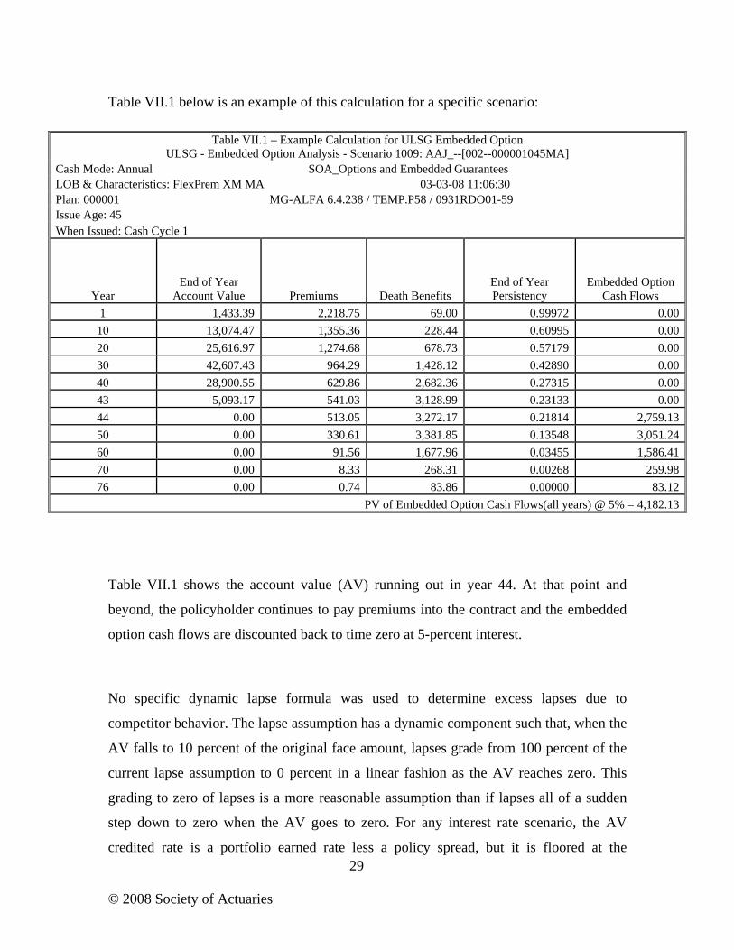
Table VII.1 below is an example of this calculation for a specific scenario:

Table VII.1 shows the account value (AV) running out in year 44. At that point and

beyond, the policyholder continues to pay premiums into the contract and the embedded

option cash flows are discounted back to time zero at 5-percent interest.

No specific dynamic lapse formula was used to determine excess lapses due to

competitor behavior. The lapse assumption has a dynamic component such that, when the

AV falls to 10 percent of the original face amount, lapses grade from 100 percent of the

current lapse assumption to 0 percent in a linear fashion as the AV reaches zero. This

grading to zero of lapses is a more reasonable assumption than if lapses all of a sudden

step down to zero when the AV goes to zero. For any interest rate scenario, the AV

credited rate is a portfolio earned rate less a policy spread, but it is floored at the

Table VII.1 – Example Calculation for ULSG Embedded Option ULSG - Embedded Option Analysis - Scenario 1009: AAJ_--[002--000001045MA]

Cash Mode: Annual SOA_Options and Embedded Guarantees LOB & Characteristics: FlexPrem XM MA 03-03-08 11:06:30 Plan: 000001 MG-ALFA 6.4.238 / TEMP.P58 / 0931RDO01-59 Issue Age: 45 When Issued: Cash Cycle 1

Year End of Year

Account Value Premiums Death Benefits

End of Year Persistency

Embedded Option Cash Flows

1 1,433.39 2,218.75 69.00 0.99972 0.0010 13,074.47 1,355.36 228.44 0.60995 0.0020 25,616.97 1,274.68 678.73 0.57179 0.0030 42,607.43 964.29 1,428.12 0.42890 0.0040 28,900.55 629.86 2,682.36 0.27315 0.0043 5,093.17 541.03 3,128.99 0.23133 0.0044 0.00 513.05 3,272.17 0.21814 2,759.1350 0.00 330.61 3,381.85 0.13548 3,051.2460 0.00 91.56 1,677.96 0.03455 1,586.4170 0.00 8.33 268.31 0.00268 259.9876 0.00 0.74 83.86 0.00000 83.12

PV of Embedded Option Cash Flows(all years) @ 5% = 4,182.13

30


guaranteed credited interest rate. The AV credited rate is uncapped and can increase and

decrease as the portfolio earned rate moves, thus potentially mitigating excess lapses due

to competitor behavior with regard to credited rate practices.

Recall that a number of different scenario sets and the times when each was appropriate

were discussed. The difference between the market consistent, long-term risk neutral and

historic scenarios can often be quite large. Table VII.2 below summarizes these

differences for a few examples.

Table VII.2 - Average PV of Embedded Option Cash Flows for Three Different Scenario Sets over 1,000 Scenarios

45, Male 65, Male Total Weighted

Scenario Set Preferred

NS Preferred

NS Liability Portfolio

Historic 5,779 15,976 11,447 Long-Term Risk Neutral 4,855 14,084 10,405

Market Consistent 2,522 10,415 7,134

One of the characteristics of market consistent scenarios is that the shape of the yield

curve determines the forward rates that will serve as the average return in arbitrage-free

stochastic scenarios. A typical upward sloping yield curve will result in forward rates

significantly higher than current rates. This characteristic is what makes the embedded

values in the above table lower for the market consistent scenarios versus the long-term

risk neutral or historic scenarios.

In the current accounting regimes, the embedded option we are valuing in this report is

handled in different ways. Statutory reserves would be determined based on Actuarial

Guideline AXXX. This guideline, like most current statutory calculations, does not

attempt to reflect current market conditions. The valuation interest rate is locked-in,

based on the issue date and the calculation is formulaic rather than stochastic. Of course,

31


cash flow testing is always an aggregate requirement that does incorporate some

stochastic features and current market conditions. Principle-based reserve methods will

be discussed in generalities later in this report.

On the GAAP side, AICPA SOP 03-1 addresses the case where additional reserves may

be required for UL-type contracts if the amounts assessed for insurance benefits are

assessed in a fashion that is expected to develop profits followed by losses. This situation

can be common in UL designs. A liability is set up at issue that recognizes a portion of

the assessments that offsets benefits to be provided in the future.

ULSG contracts are subject to SOP 03-01, stated in paragraph 3. The methodology of

SOP 03-1 results in the development of a “benefit ratio,” which is defined, at issue, as the

ratio of the present value of the excess benefits to the present value of policy assessments.

Policy assessments usually include policy loads, surrender charges, COIs, and investment

spread, but excess benefits may not have a clear definition. Once the benefit ratio is

determined, the additional reserve is a retrospective accumulation with interest of policy

assessments collected, multiplied by the benefit ratio minus any excess benefits paid

during the accounting period.

In a recent Milliman survey, respondents discussed the implementation challenges of

SOP 03-1. There was not an overriding consensus on what the assessment was after the

account value went to zero, answers included zero or the stipulated premium. Most

respondents agreed the benefit in this situation was the death benefit. The definition of

excess benefits was more problematic and answers included the death benefits paid after

the account value goes to zero, the death benefits paid, less the reserve released, after the

account value goes to zero, or some function of the income statement losses. Scenarios

generated to project assessments and excess benefits were a mix of historic and market

consistent scenarios. The discount rate used was consistent with the rate used to amortize

DAC. The AAA practice note on SOP 03-01 provides some interpretation of the

32


requirements of SOP 03-01 to help companies perform these evaluations, but it does not

provide clear answers to the issues stated above.

The evaluation of the additional reserve for this project is grounded in evaluating the

embedded option in a market consistent scenario framework. Present values of death

benefits paid less the stipulated premiums, after the primary account value goes to zero,

are averaged over many stochastic paths where the embedded option cash flows are

discounted using the one-year rates along each stochastic path. This process would be

performed at each future valuation date and the results would be added to the base

reserve at each valuation date.

33


VIII. Attribution Analysis

The calculated value for the embedded option is important, but on its own provides little

insight into the nature of the liability. To really understand the value, to assess the

reasonability and to determine what conditions will cause the embedded value to change,

an attribution analysis can be helpful.

An attribution analysis, as defined here, will look at the change in the embedded option

value over a period of time and break the change into components. It is often the case that

the entire change cannot be explained as part of the attribution analysis. The point of the

attribution analysis is to show how the major drivers of the value flowed through the

change in the embedded option value.

VA with GLWB - Sources of Volatility that Combine to Determine Volatility of the

Embedded Option Values

• Interest Rates: Interest rates impact the embedded option value in a few ways. First,

most variable annuities have a variety of fixed income investment options as well as a

fixed account. An increase in interest rates may have a short-term effect on the value of a

fixed income subaccount, but also may have a long-term impact on higher subaccount

returns.

The second way interest rates impact the embedded option value is in discounting future

benefits. Since most GLWB benefits will be far out in the future, the discount rate can

have a significant impact on the present value.

The third way significantly impacts the market consistent embedded value calculation.

Since the current interest rate environment is used to calculate forward rates that are the

34


mean growth rate in future periods, relatively small changes in interest rates and/or the

shape of the curve can have a major impact on the projected future benefits and the

embedded value calculation.

• Equity Returns: Directional movements in the market will have an impact on the

embedded value calculation. Positive equity returns will reduce the value of the GLWB

liability. In the early contract durations, the impact of equity returns is small relative to

the impact of interest rate changes. As the contract ages and as the GLWB potentially is

more and more in-the-money, the impact of equity returns becomes more significant.

• Implied Volatility: In a market consistent embedded value calculation, implied

volatilities are used as the volatility assumption in the stochastic scenarios. Increases in

implied volatility, particularly in the early years, can have a significant impact on the

liability.

• Policyholder behavior: The various policyholder behavior assumptions required to

perform the stochastic modeling all have an impact on determining the embedded values.

The lapse assumption typically includes a dynamic lapse component that reduces the

lapses as the GLWB becomes more in-the-money. The combination of the base lapse

assumption and this dynamic component determine the projected number of contracts

available to use the GLWB. Other assumptions such as mortality and withdrawal rates

also impact the embedded value calculation. To the extent these assumptions do not

match experience, the attribution analysis can demonstrate the portion of the change in

the embedded value caused by the difference between assumption and experience.

35


ULSG - Sources of Volatility that Combine to Determine Volatility of the Embedded

Option Values

• Interest Rates: As interest rates fluctuate, so do the cash flows and the valuations of

existing and new assets that determine overall portfolio yields when credited interest rates

are driven by a portfolio earned rate approach. As the yield curve changes from period to

period, at a particular valuation date a new set of risk-neutral scenarios are developed,

which may cause the embedded option cash flows to change. Also, discount rates (one-

year rates are used) are likely to change and are dependent on the new level and shape of

the yield curve at the current valuation date. An example is provided in this section

explaining this situation and implications in more detail.

• Policyholder Behavior: Policyholder behavior through disintermediation, additional

premium payments, or stopping premium payments, can add to the difficulty of valuing

the embedded option. As the uncertainty of policyholder behavior increases, assumption

development to value the embedded option becomes more difficult and the need for

sensitivity testing increases in order to evaluate embedded optionality appropriately.

Embedded Option Attribution Example

GLWB Example

For the GLWB product the attribution analysis is completed by relying on the sensitivity

of the embedded option based on the various measures of the Greeks.

In the following example, the value of the GLWB embedded option was determined at

time 1 and time 2 of scenario 3,178 of the C3 Phase II pre-packaged scenarios from the

AAA. At each valuation point the yield curve is converted to forward rates. These rates

along with the implied volatility surface and correlation matrix are utilized to develop

36


market consistent scenarios. In this example, to project forward and obtain the present

value of the liabilities, 250 market consistent scenarios were developed. The value of the

liability at time 1 was $2,989, and the value of the liability at time 2 was $2,510. Table

VIII.1 shows the index value of the various funds and the average forward rate at both of

these times.

Table VIII.1: Index Values of Funds At Various Times

Time 1 Time 2 Change S&P 1,091 1,069 -2.0% Russell 1,520 1,485 -2.3% NASDAQ 840 727 -13.5% SBIG 1,049 1,058 0.9% EAFE 1,010 1,046 3.5% Money Market 1,034 1,074 3.9% Total Allocation 1,123 1,112 -0.9% Average Fwd Rate 4.70% 5.16% 0.46%

At time 1 various measures of the Greeks were also developed to measure the sensitivity

of the value of the liability to changes in the economic environment. To calculate the

Greeks it was necessary to repeat the process of valuating the liability changing one input

of the scenario generator at a time. In this example, the process was repeated 16 more

times to obtain the delta, rho and vega values of the liability.

The delta measure is the sensitivity of the value of the liability with respect to changes in

price of the underlying funds. To calculate this measure, each of the six funds was

shocked up and down by 1 percent independently. For each fund, the delta is equal to the

average difference between the two values. In this example, the value of the liability

adding 1 percent to the S&P fund is 2,979.43. The value of the liability reducing the S&P

fund by 1 percent is 2,997.60. The value of the delta for this fund is

then ( ) 09.92

2,997.60-2,979.43−= .

37


Since this embedded option can be viewed as a put option, it is expected that the value of

the delta will be negative. It is also expected as this option gets more in-the-money that

the value of the delta will be more negative, hence more sensitive to small changes in the

underlying funds. Chart VIII.1 shows the liability values at time 1 and the deltas for each

of the underlying funds as well as the delta for the overall allocation.

Chart VIII.1: Embedded Option Deltas and Option Values

GLWB Embedded Option Deltas

2,950

2,960

2,970

2,980

2,990

3,000

3,010

3,020

3,030

Opt

ion

Valu

e

Delta -9.09 -7.05 -3.52 -3.90 -7.40 -5.99 -36.95

1% Dow n 2,998 2,996 2,992 2,993 2,996 2,995 3,025

1% Up 2,979 2,981 2,985 2,985 2,981 2,983 2,951

No Change 2,989 2,989 2,989 2,989 2,989 2,989 2,989

S&P Russell NASDAQ SBIG EAFE MM All Funds

The rho measure is the sensitivity of the value of the liability with respect to moves in

interest rates. To calculate this measure a parallel shift in the 1 year forward curve of 0.1

percent up and down was assumed and the liability was revalued. The value of the

embedded option with a 0.1-percent increase in interest rates is 2,854.98. The value of the

embedded option with a 0.1-percent decrease in interest rates is 3,128.48. The value of

rho is then calculated in the same way as the values of the deltas were by averaging the

change of the two values. In this example the value of rho is ( ) 75.1362

3,128.48-2,854.98−= .

Rho is larger for embedded options that are in-the-money, and is also larger as the time to

exercise is farther away. As the time to exercise gets shorter the value of rho gets smaller.

38


These two effects are the consequence of longer discount periods and larger amounts of

the liability as the embedded option is more in-the-money.

In real life, the yield curve does not move in parallel shifts as the assumption made to

measure rho in this example. Therefore, in practice, it is possible to shock different points

on the yield curve to obtain a more accurate measure of the change in the liability due to

changes in interest rate.

The vega measure is the sensitivity of the value of the liability with respect to moves in

the implied volatility. To calculate this measure a parallel shift to the volatility surface of

1 percent up and down was assumed and the liability was revalued. The value of the

embedded option with a 1-percent increase in implied volatility is 3,165.99, while the

value of the embedded option with a 1-percent decrease in implied volatility is 2,815.94.

Using the same logic to value the change in liability used for the other measures, the

value of vega is ( ) 03.1752

2,815.94-3,165.99= .

The Greeks can be used to approximate the value of the liability given the changes in the

underlying assumption, and therefore to attribute the change in the embedded value from

period to period. As an example of how to calculate the change in embedded option value

from one period to the next using the Greeks, consider rho. In this example, the value of

rho is -136.75 for every 0.1-percent change in the interest rates. The interest rate changed

from period 1 to period 2 by 0.46 percent, so the approximated change in option value

from period 1 to period 2 due to the changes in interest rates is 07.63175.136*%1.0%46.0

−=−

(value differs due to rounding). Similarly the rest of the adjustments can be calculated.

39


Table VIII.2 shows the change in value of the embedded option by attribute.

Table VIII.2 – Change in Value of Embedded Option

Amount Greek Measure Change in

Assumption Option Value at time 1 2,988.69 S&P Adjustment 18.37 -9.09 -2.0%Russell Adjustment 16.02 -7.05 -2.3%NASDAQ Adjustment 47.57 -3.52 -13.5%SBBIG Adjustment -3.38 -3.90 0.9%EAFE Adjustment -26.13 -7.40 3.5%MM Adjustment -23.17 -5.99 3.9%Sum of individual fund adjustment 29.28 Delta (Equity) Adjustment 34.59 -36.95 -0.9% Rho (Interest) Adjustment -631.67 -136.75 0.46% Vega (Volatility) Adjustment 0.00 175.03 0.0% Discount (Theta) Adjustment 123.18 1 yr fwd rate = 4.1% Total Adjustment -473.90 Attributed Option Value 2,514.79 Actual Option Value 2,509.85 Percent of Change Explained by Attribution Analysis 99.0%

The Greek measures are good at predicting small changes in the underlying attributes.

When changes in these attributes are large, for example the changes in the NASDAQ

fund of -13.5 percent, other measures are necessary to improve the approximation of the

option value. This can be seen in our example with the discontinuity of the sum of the

changes due to individual funds of 29.28 versus the calculation of the changes to the

option value on the overall allocation of equity of 34.59. Calculating gamma (the change

40


in delta) would improve the adjustment to the option due to the individual changes in the

funds, and the two figures presented prior would be closer to each other.

Another measure worth mentioning at this time is theta. Theta measures the sensitivity of

the embedded option as time passes. In our example, the value of theta is calculated by

the amount of interest needed to accumulate the option value from period 1 to period 2.

ULSG Example

Chart VIII.2 presents the yield curves that are used in the embedded option valuation and

attribution examples that follow. The yield curve at time t = 1 steepened by 75 bps at the

10-year maturity with smaller increases on the shorter end of the yield curve. Parallel

yield curve shifts, to the yield curve at time t = 0 , of +/-100 bps are also shown.

Chart VIII.2: Yield Curves

Yield Curve Shifts

2.5%3.0%3.5%4.0%4.5%5.0%5.5%6.0%6.5%

90d 180d 1y 2y 3y 5y 7y 10y 20y 30y

Maturities

Yie

ld R

ates

Yield Curve(t = 0) Yield Curve(t = 1) Yield Curve(t = 0) + 100 bps Yield Curve(t= 0) - 100 bps

Chart VIII.3 below exhibits the valuation of the embedded option for all new business

cells at time t = 0 and time t = 1 where the yield curves (using the above yield curves at

time t = 0 and time = 1) are shocked by +/-100 bps and +/- 200 bps to assess the volatility

of the embedded option values given that a steepening of the yield curve has occurred

41


Graph VIII.3: Valuation of Embedded Option of New Business

Embedded Option Value

0

5,000

10,000

15,000

20,000

25,000

0 1Duration

-200 bps -100 bps No change +100 bps +200 bps

At each duration and yield curve shift a new set of 500 risk-neutral scenarios was

developed, which causes embedded option cash flows to change. In the graph above at

time t =1, the yield curve steepened and projected forward rates are higher than they were

at time t = 0. These forward rates seed the risk-neutral interest rate generator, in general

projecting higher interest rates, which imply that the embedded option value should

usually be lower than it was at time t = 0. This decreased embedded option value stems

from higher credited rates driving higher account values making the embedded option

more out-of-the-money (account value is positive longer pushing embedded option cash

flows further out) and higher discount rates are used to value those option cash flows .

Table VIII.3 below is an example using option risk measures to attribute the change in

embedded option value from period to period.

42


Table VIII.3 – Change in Embedded Option Valuation Using Option Risk Measures

Embedded Option Values and Option Risk Measures Yield Curve

Shift(parallel) Time 0 Time 1 Change -100 bps 12,837 No change 8,115 5,997 (2,118) +100 bps 4,954 Rho -48.57 Effective Convexity 1,924.15

Option Value Option Value Change Change using

10 Year Yield Change (bps) using Rho Convexity +75 -2,956 439

Partial Durations

Rate Partial Embedded Yield Curve Maturity Change (bps) Durations Value Change

1 year 28 -0.12 -3 10 year 75 26.83 1,633 30 year 75 -74.71 -4,547

-2,917 Embedded Option Value Attribution

Option Value(t=0) 8,115 Option Value change due to:

+ Rho(t=0) Adjustment -2,956 + Convexity(t=0) Adjustment 439 + Discounting Adjustment 392 = Estimated Option Value(t=1)

5,990

% of Actual(t=1) = 99.9%

+ Lapse Adjustment -47 = Estimated Option Value(t=1)

5,943

% of Actual(t=1) = 99.1%

43


In the attribution example above, a valuation at time t = 0 of the embedded option

produces a value of $8,115. To approximate the embedded option value change from

time t = 0 to time t = 1, a couple of option risk measures were determined. The yield

curve at time t = 0 was shifted up and down by 100 basis points to calculate a rho of -

48.57 (sign convention consistent with the option value change when rates rise),

essentially an effective duration calculation, which generates a 48.57-percent or a $2,956

decrease in option value for the 75 basis-point (bp) increase in rates at the 10-year

maturity.

Embedded option value changes exhibit a convexity relationship as can be seen by the

asymmetric relationship of the calculated embedded option values after the +/- 100 bps

parallel shifts of the yield curve. As stated previously, as rates increase, account values

increase and the embedded option becomes more out-of-the-money as the account value

will be positive longer. Similarly, as rates decrease, account values decrease and the

embedded option becomes more in-the-money as the account value depletes faster. The

amount of convexity in the option value depends on how fast the growth or the depletion

occurs when rates change, relative to the no shift case, how the policy has aged, and

where the floor is on the credited interest rate. The effective convexity was approximated

as (12,837 + 4,954 - 2 x 8,115) / [8,115 x (.5 x .02)^2] = 1,924.15 (actual unrounded).

The approximation for effective convexity used equals (P- + P- - 2 x P0) / [P0 x (.5 x (y+ -

y-))^2] , where “+” indicates a +100 bps parallel shift and “-” indicates a -100 bps parallel

shift in the yield curve, P is the option value, and y is the interest rate. For this example,

the embedded option exhibits positive convexity and the effective convexity generates a

.5 x 1,924.15 x 8,115 x (.0075) ^ 2 = $439 increase in embedded option value at time t =

0 assuming a 75 basis point (bp) increase at the 10-year maturity.

Rho and effective convexity together predict an embedded option value of $5,598 at time

t = 1 or approximately 93.3 percent of the calculated option value of $5,997 at time t = 1.

44


Since the embedded option has a finite number of cash flows, given no change from time

t = 0 to time t= 1 except for a small change in account values, the embedded option value

would grow by embedded option value (t = 0) x discount rate (year 1) = $392. Rho,

effective convexity, and the discounting adjustment predict an embedded option value of

$5,990 at time t = 1 or approximately 99.9 percent of the calculated option value of

$5,997 at time t = 1.

Suppose that over the year from time t = 0 to time t = 1, lapse experience was 25 percent

higher than expected and that the embedded option value at time t = 1 does incorporate

this assumption. Assuming an overall weighted lapse rate of 8.9 percent, the lapse

adjustment of .089 x .25 x (-2,956 + 439 + 392) = $ -47 should be added to the embedded

option value estimate of $5,990 at time t = 1 giving an estimate of $5,943 or

approximately 99.1 percent of the calculated option value of $5,997 at time t = 1.

Rho and effective convexity option risk measures are generally used to approximate

option values for small instantaneous movements in rates. This example shows that these

measures can be used as a way to predict a substantial amount of the change in embedded

option value from period to period to a reasonable degree of accuracy.

The actual yield curve change from time t = 0 to time t = 1 was not a parallel shift up +75

bps. A yield curve steepening occurred on the long end of +75 bps with smaller yield

changes for the shorter maturities. The 10-year rate served as the rate used in the

attribution since the 10-year rate was the primary driver of portfolio earned rates, which

drive credited interest.

Partial durations were calculated to assess the sensitivity of the embedded option to non-

parallel shifts in the yield curve. Partial durations were determined at three key

maturities. The change in the embedded option value using only the partial durations was

-$2,917 versus -$2,956 (using Rho and the 10-year rate change to approximate the

change in embedded option value which assumes a parallel shift in the yield curve).

45


For the example above, the embedded option was evaluated at issue and at one year out

and the sensitivity of the embedded option value is primarily driven by the long part of

the yield curve as can be seen by the 30-year partial duration of -74.71. This relationship

makes sense since the embedded option has very long-dated cash flows for a newly

issued policy and the late duration credited rates really determine whether the option is

in- the- money or not. Early duration credited rates are less important as the COI charges

dominate due to high net-amounts-at-risk.

The 10-year partial duration at issue is positive. Credited interest rates are a function of a

moving average of 10-year rates, but early duration COI charges predominantly dominate

and the late duration credited rates are more important to the sensitivity of the embedded

option values.

Chart VIII.4 below exhibits the progression of the 10- and 30-year partial durations.

Chart VIII.4: Progression of the 10 and 30-year Partial Durations

Progression of Partial Durations

-80-70-60-50-40-30-20-10

0102030

1 3 5 7 9 11 13 15 17 19 21 23 25 27 29

Duration

Part

ial D

urat

ions

10 yr Partial Duration 30 yr Partial Duration

46


As the policy ages, the point at which the sensitivity of the embedded option becomes in-

the-money moves closer to the current valuation date. For example, in the early durations

of the block, the long part of the curve (maybe 25-30 years out) is the most important

driver of embedded option value changes. If the block has aged 20 years or so, the longer

part of the curve becomes a less dominate driver of the change in embedded option value.

The convergence of the 10 and 30-year partial durations in Chart VIII.4 exhibits this

characteristic.

47


IX. Longitudinal Analysis

The prior section demonstrated the importance of understanding the items that influence

the change in the embedded option value. This section will examine how the sensitivity

of the embedded option varies over time and based on market conditions. It is important

to understand these items so that fluctuation in the embedded option value can be

anticipated and explained.

GLWB Example

The GLWB example below uses a specific stochastic scenario to observe the sensitivity

of the embedded option to the various drivers over time and over various market

conditions.

Chart IX.1 below is a graph of the scenario. In this scenario, interest rates rise

substantially over the first 9 years and then fall dramatically over the next two years.

Equity performance is generally favorable in this scenario other than the flat period

between years 10 and 20.

48


Chart IX.1: Interest Rate Scenario

Economic Scenario

0%

1%

2%

3%

4%

5%

6%

7%

8%

9%

10%

1 2 3 4 5 6 7 8 9 10 11 12 13 14 15 16 17 18 19 20 21 22 23 24 25 26 27Years

Yie

ld C

urve

Val

ue

0

500

1,000

1,500

2,000

2,500

3,000

3,500

4,000

Equi

ty In

dex

Val

ue

1 Yr Yield 5 Yr Yield 10 Yr Yield Equity

Chart IX.2 below shows the relevant Greeks for the GLWB embedded option through

this scenario. The graph also shows the embedded option value. The embedded option

value falls quickly over the first six years largely due to the rapid increase in interest

rates. The embedded option then climbs overtime.

A pattern that is typical to this type of analysis is apparent in the following graph. The

sensitivity to interest rate (rho) and implied volatility (vega) starts high and then

grades toward zero as the date for paying (or not paying) any GLWB payments

approaches. This makes sense because as the ultimate benefit amount is approached,

the average rate of fund growth (determined by interest rates) and the fund growth

volatility are less important.

49


Chart IX.2: GLWB Embedded Values

GLWB Embedded Values

-200

-150

-100

-50

0

50

100

150

200

1 2 3 4 5 6 7 8 9 10 11 12 13 14 15 16 17 18 19 20 21 22 23 24 25 26Years

Gre

ek V

alue

0

500

1,000

1,500

2,000

2,500

3,000

3,500

Embe

dded

opt

ion

Val

ue

Delta Rho Vega Embedded Option

ULSG Examples

Chart IX.3 below shows the evolution of embedded option values for the block of cells

for three deterministic scenarios, each scenario starts with the 9/30/07 swap curve. The

flat scenario has future rates held at the initial yield curve rates, the increasing scenario

has rates increase by 15 bps per year for each yield curve maturity, and the decreasing

scenario has rates decrease by 15 bps per year for each yield curve maturity. The 15 bps

increases and decreases occur over each duration of the 30-year scenarios. A set of 300

risk-neutral scenarios were generated at each valuation date to value the embedded

option.

50


Chart IX.3: Evolution of Embedded Option Values for Three Scenarios

Embedded Option Values

010,00020,00030,00040,00050,00060,00070,000

1 4 7 10 13 16 19 22 25 28Duration

Flat Increasing Decreasing

As can be seen the first embedded option value is the same for each of the three

scenarios, since each scenario has the same initial yield curve. Embedded option

values slowly increase for the flat scenario. For the decreasing scenario, embedded

option values rise faster than the flat scenario due to decreasing credited and

discounting rates. For the increasing scenario the opposite occurs, embedded option

values decrease faster than the flat scenario due to rising credited and discounting

rates.

Chart IX.4 below shows absolute values of rho under the increasing and decreasing

scenarios described above. An interesting phenomenon in the early durations is that

the value sensitivity of the embedded option is larger in the increasing versus

decreasing scenario. Credited interest rates were floored at 3.0 percent, so this will

effectively limit the amount of embedded option cash flows in a down scenario and

this dampens the volatility of the embedded option values to some degree (i.e. when

51


rho is calculated at a valuation date, the current yield curve is shocked +/- 100 bps to

determine rho).

Chart IX.4: Absolute Values of Rho under Increasing and Decreasing Scenarios

Absolute Value of Rho

0

10

20

30

40

50

1 3 5 7 9 11 13 15 17 19 21 23 25 27 29

Duration

Increasing Decreasing

Chart IX.5 below shows the evolution of embedded option values for the block of cells

for a C3-Phase II scenario. A set of 300 risk-neutral scenarios were generated at each

valuation date to value the embedded option.

52


Chart IX.5: Evolution of Embedded Option Values for C3-Phase II Scenario

Economic Scenario

0%

2%

4%

6%

8%

10%

12%

14%

1 3 5 7 9 11 13 15 17 19 21 23 25 27 29Duration

Yiel

d Le

vel

0

5,000

10,000

15,000

20,000

25,000

Embe

dded

Val

ue

1 Yr Annual Yield 10 Yr Annual Yield Embedded Option Value

The embedded option value changes are essentially consistent with the movements of

the 10-year rates. In general, as the 10-year rates increase (decrease), embedded option

values decrease (increase). For this more realistic interest rate scenario, as compared to

the deterministic scenarios above, the determined embedded option values are quite

volatile. Incorporation of the embedded option values into reserves for a pricing

exercise would necessitate a stochastic framework to properly evaluate the embedded

optionality. A balance needs to be struck between the number of risk-neutral scenarios

to run at each valuation date as well as the number of pricing scenarios (outer loop

scenarios) to use as the exercise is computationally intensive, but well suited for a grid

computing platform.

53


X. Integration into Pricing

One of the questions this research report intended to answer has to do with how the value

of the embedded option can be integrated into pricing. Stochastic pricing has been used in

insurance product pricing for many years to estimate the range of potential results.

Stochastic analysis has been facilitated by improvements in technology, namely

computing power. The kinds of stochastic analysis done today could not have been

contemplated 20 years ago.

The emergence of stochastic analysis in pricing primarily started with products that had

obvious sensitivity to interest rate movements. For instance, it has long been understood

that fixed annuity policyholders were more likely to lapse when the crediting rate on their

current product is less than prevailing market rates. This is called disintermediation lapse.

Since an insurance company generally buys bonds with five- to seven-year maturities to

back an annuity with a seven-year surrender charge schedule, a large number of lapses in

a market where interest rates have risen significantly would result in capital losses from

the forced asset sales to cover the lapse payments. This type of a dynamic is impossible

to see in a single-level interest rate environment scenario. Stress test scenarios like the

“New York 7” can show these dynamics, but may be too extreme to allow the pricing

actuary to assess the risk of this type of behavior.

As variable products became more popular and especially as guarantees on variable

products became common place, stochastic analysis became a core component of the

product pricing effort. Rather than being a secondary test to evaluate the potential range

of values, stochastic analysis became the tool for setting prices. In the early emergence of

guarantees on variable products, stochastic analysis was done using historic scenarios and

then setting a price so that the cost would be covered in 80 to 90 percent of the scenarios.

More recently, the focus has been on calculating the cost to hedge the guarantee. This

type of analysis focuses on average claim costs under risk-neutral scenarios.

54


With the advent of C3 Phases 1 and 2, VACARVM, and principle-based reserves, future

reserves and capital requirements are no longer generally known, or at least not easily

calculated based on a specific projected path, at issue. This has forced the pricing actuary

to consider stochastic-in-stochastic methods for generating the range of cash flows and

profitability that will emerge from a product.

As attention shifts to topics like economic capital and enterprise risk management,

actuaries are being asked to assess how a new product initiative would look in the context

of a company’s existing balance sheet and the risks the company currently faces. This

becomes an exercise in stochastically modeling a new product in conjunction with the

entire company. Obviously the expectations of the pricing actuary and the models used

by the pricing actuary continue to advance.

In the context of the pricing implications of this research project, if the focus is placed on

the results generated by the market consistent scenarios, the value of the embedded

option can be thought of as the price the insurer would have to pay to remove the liability

from its balance sheet. If the embedded option value calculated here is added to or

integrated with all the other embedded options in the contract and this sum is added to the

realized value in the contract, for which the cash value is a good proxy, we have a sum

that is representative of the total fair value of the liability.

Suppose that this fair value of the liability was used as the reserve in a typical income

statement and the assets backing the reserve were in two forms. The assets backing the

cash value could be typical fixed income assets. The assets backing the embedded value

would be the appropriate hedge instruments to match the market consistent embedded

value. These hedge assets would transfer the risks associated with the embedded option to

the capital markets. The insurer would be left with a low risk product. If all embedded

options were accounted for, the product could be thought of as no risk.

55


The income statement generated by this approach would result in projected cash flows.

These cash flows could be discounted to calculate a profit margin. If these cash flows

were discounted at the risk-free rate under the assumption that all embedded options are

accounted for, then a reasonable expectation would be a zero profit margin. Any amount

in excess of this would be an excess return in a no-risk situation.

The pricing approach described above is not generally how companies would ultimately

determine a price for a product for two reasons. First, it is difficult to measure all

embedded options and second, insurers are in the business of taking on risk and getting

paid for taking on this risk. However, the pricing method above could be thought of as a

secondary threshold, which would confirm that if all embedded options were transferred

to the capital markets, the product would still return the risk-free rate. Since insurance

companies are in business to earn more than a risk-free rate of return, appropriate risks

need to be taken and compensated for so that the overall return will be some reasonable

margin above the risk-free rate of return.

An examination of embedded options and their sensitivities can also provide insights into

risks that can be mitigated through diversification and ones that cannot. For instance,

given a large enough population, the risks associated with an individual’s mortality are

diversifiable, while over-all trends in population mortality are not. Risks associated with

the interest rate environment and equity markets overall can often be hedged reasonably

efficiently but are generally not diversifiable. Knowing the risks associated with the

embedded option allows the insurance company to assess the cost of hedging, keeping or

seeking to diversify these risks.

ULSG Example of Pricing Regime

Embedded option values were incorporated into reserves to assess profitability under 200

C3-Phase II scenarios (outer loop scenarios). Pre-tax profit margins were captured for

each scenario where pre-tax profits and premium were discounted at the one-year rates at

56


each duration. The reserve equals the cash value + embedded option value at each

duration. The reserve can be thought of as two independent pieces: (1) Cash value is for

the primary guarantee in that the policy will stay in force as long as the cash value is

positive, and (2) The embedded option value is for the secondary guarantee when the

cash value is depleted and the primary guarantee lapses, but the policy stays in force as

long as the policy’s secondary guarantee requirements are met. Essentially this exercise is

a market consistent evaluation of statutory pre-tax profits where the product design has

not been modified.

As discussed above, it is expected that the average of the pre-tax profit margins will be

close to zero. The average pre-tax profit margin for this calculation was 48 bps of the

present value of premiums. This is significantly lower than a typical pricing profit margin

for a ULSG product. Taxes are a confounding factor in this exercise and were ignored.

One of the challenges of creating results like those above is the stochastic-in-stochastic

issue. The results above are based on a set of “outer-loop” stochastic scenarios that are

historic scenarios. Along each of these stochastic scenarios, an “inner-loop” is taking the

economic environment based on the outer-loop scenario to generate a set of market

consistent scenarios. These inner-loop scenarios are used to value the embedded option.

One of the major challenges of this type of analysis is run-time. This stochastic-in-

stochastic run has a huge number of computations to perform. While grid computing

systems can spread stochastic-in-stochastic runs over many processors, there still is a

tremendous amount of data created that has to be summarized in the results. It is essential

to have a high degree of confidence in the model before attempting stochastic-in-

stochastic runs, as it is unfeasible to perform detailed calculation checks. However, the

types of attribution analysis described in Section VIII of the report can provide a certain

level of comfort that the model is working correctly.

57


XI. Comparison to Similar Calculations

Many of the calculations actuaries perform are migrating from relatively straightforward,

although often complex, formulaic calculations to calculations that involve stochastic

models. C3 Phase I, C3 Phase II, principles-based reserves (PBR), FAS 133, FAS 157,

international financial reporting standards (IFRS) and market consistent embedded value

(MCEV) all rely on stochastic analysis.

The first three items on the above list are statutory measures focused on company

solvency. All three of these calculations rely on historic scenario sets with an amount of

conservatism added. The primary calculation for each of these involves the accumulation

of surplus. The accumulated surplus is examined each year within the stochastic

projection to confirm sufficiency along that path or to determine the additional amount

needed if not sufficient. The final calculation looks at any additional surplus required for

each scenario and calculates the average of a certain portion of the worst scenarios (e.g.

90 CTE is the average of the worst 10 percent of scenarios).

The statutory solvency focus of C3 Phase I, C3 Phase II, and PBR is very different from

the primary calculations we have been using in this report to examine the embedded

option. First, our calculations have centered on the present value of specific cash flows.

This focus does not attempt to address sufficiency of the interim amount of surplus.

Second, the three statutory measures use historic based scenarios to generate future

values. Third, our embedded option calculations involved the average of the individual

scenarios rather than concentrating on the tail of the distribution the way the statutory

solvency focused calculations do.

The next two measures, FAS 133 and FAS 157, are GAAP measures explicitly for

determining the value of embedded derivatives. The methodology of these calculations is

to rely on market consistent methods to assess the value of the embedded derivative. This

58


generally is consistent with the methods used in this report. One exception is that GAAP

uses adjustments to ensure certain characteristics. For instance, the starting GAAP

reserve has to equal the amount received by the insurance company. For our GLWB

contract, the $50,000 premium would start a $50,000 account value that would be a part

of the GAAP reserve. Any additional reserve for the embedded option generally needs to

equal zero at the moment of issue. This is done by computing an imputed charge such

that the present value of future benefits minus the present value of future imputed charges

equals zero at issue.

For the last two items, IFRS and MCEV, the similarities between these methods and the

methods in this report seem to be the strongest. IFRS is yet to be fully defined but it

seems to be moving toward a fair value type calculation, where the entire liability is

measured on a market consistent basis of some form. This is really a step beyond the

valuation of the embedded option described in this report.

MCEV relies on the bifurcation of the liability into an embedded option and a host

contract. The host contract is valued using a formulaic method. The embedded option is,

as the name implies, valued on a market consistent basis. This is very similar to the

methodology described in Section X.

59


XII. Conclusions

At the beginning of this report we set out to answer a number of questions. The first

question was whether closed-form solutions could be used in assessing the value of the

embedded option. An example was shown for a relatively simple GMAB on a variable

annuity. It was demonstrated that a closed-form solution could be used for this relatively

simple guarantee. The point was then made that for more complicated products such as

GMWBs and ULSG products, no closed-form solution existed.

One advantage of closed-form solutions is that they do not have stochastic runtime issues.

This can be especially beneficial in a stochastic-in-stochastic situation where the inner-

loop stochastic could potentially be avoided. However, with the ever increasing

complexity of the products being sold, it does not appear that expecting a closed-form

solution for each type of liability is reasonable.

The second question had to do with generating stochastic scenarios. The paper described

three different types of stochastic scenarios: historic, long-term risk neutral and market

consistent. The paper discussed and demonstrated how parameters could be set for each

of these models and, in the case of the Market Consistent models, how the resulting

scenarios could be validated relative to prices observable in the marketplace.

For the two products used in this paper, each of the three scenario sets was used to

calculate values. The paper showed that the value of the embedded option is highly

sensitive to the scenario set used. The paper also discussed the situations where each of

the values might be appropriate.

The third question was in regard to liability assumptions. In describing the two products

used in this report, the assumptions that were used in calculating the embedded value

were described in detail. The rationale behind the assumptions was also discussed.

60


However, the paper also mentioned that often there is little or no historic data that can be

used to set these assumptions and this is where judgment needs to come into play.

Judgment, combined with conservatism and an appreciation for the sensitivity of the

results due to a change in the assumption, is often the best an actuary can do.

The fourth and likely the most significant question was regarding validating and

understanding the results. The paper made the point that the embedded option value itself

had value, but only limited value to a company without an understanding of the items that

influence the value and an understanding of the period-to-period change in the value. A

significant portion of the paper was spent on an attribution analysis demonstration. The

attribution analysis was used to explain period-to-period changes in the embedded option

value by breaking the change into pieces that captured the sensitivity of the embedded

option value to changes in market levels, interest rates, volatility assumptions and

policyholder behavior.

Discussing ways to validate and understand the embedded option value is certainly where

we see this research report adding the most value. The authors of this report believe this

to be a critical issue as the insurance industry and the actuarial profession continue to

progress toward stochastic measures of reserves in either a principle-based framework or

with regard to International Financial Reporting Standards (IFRS). Without an ability to

understand and validate how complex embedded options will behave in these stochastic

environments, it would be difficult for an actuary to be comfortable with the stochastic

generated embedded option value results. Also, if results cannot be understood and

validated, how can actuaries hope to communicate the results to upper-management,

industry analysts, rating agencies and regulators?

The authors of this report hope that you have found information and insights that can be

applied to your particular situation. Please feel free to contact us if you have questions

and/or comments.

61


XIII. Bibliography Angstman, Clifford, G. Geoffrey Alaishuski; The Greeks; www.soa.org/files/pdf/02-

Various-TheGreeks.pdf Bennett, Tim E., Timothy E. Hill; Better Pricing in an Uncertain World; Society of

Actuaries Record, Volume 30, Number 3, Annual Meeting and Exhibits, New York, N.Y., October 2004.

Chan, Wai-Sum; Some Simple Stochastic Models for Analyzing Investment Guarantees;

Department of Statistics & Actuarial Science, University of Hong Kong, November 2003.

Chueh, Yvonne C.M.; Efficient Stochastic Modeling for Large and Consolidated

Insurance Business: Interest rate Sampling Algorithms; North American Actuarial Journal, Volume 6, Number 3, pages 88 – 103.

Hancock, Geoffrey; Stochastic Pricing, Session 62 TS, Society of Actuaries Annual

Meeting, New York, N.Y., November 2005. Hardiman, Nathan, Rebecca Scotchie; Real World Applications of Stochastic Models;

Southeast Actuaries Conference, June 2005. Lebel, Dominique, Geoffrey H. Hancock, Jeffrey A. Leitz; Risk-Based Capital

Requirements on Variable Annuities with Guarantees; Society of Actuaries Record, Volume 29, Number 3, Annual Meeting, Orlando, Fla., October, 2003.

Manistre, B. John, Geoffrey H. Hancock; Variance of the CTE Estimator; North

American Actuarial Journal, Volume 9, Number 2, April 2005. McMillan, Henry M., Douglas L. Robbins, David M. Walczak; Measuring and Pricing

for Tail Risk; Society of Actuaries Record, Volume 30, Number 2, Spring Meeting, San Antonio, Texas,, June 2004.

Ryan, Craig; Stochastic Pricing A Variable Annuity Case Study, Session 62 TS, Society

of Actuaries Annual Meeting, New York, N.Y., November 2005.

http://www.soa.org/files/pdf/02-Various-TheGreeks.pdf

http://www.soa.org/files/pdf/02-Various-TheGreeks.pdf

62


Appendix A – Universal Life with Secondary Guarantee Specifications and Assumptions

Base Universal Life Product Specifications

Account Value Loads 7.0% of premium, all years

$1.20 per unit, years 1-20

$7.50 per month, all years

Cost of Insurance (COI) Charges Typical reverse select & ultimate schedule

Guaranteed COIs 2001 CSO, Ultimate, M/F, NS/SM, ANB mortality table

Maturity Age 121

Minimum Guaranteed Interest Rate

3.0%

Surrender Charges Maximum allowable year 1 based on 2001 CSO, Ultimate, M/F, NS/SM, ANB mortality, 3.00% interest (including reduction for any “initial acquisition expense charge”). Amortization period = 19 years, zero surrender charge for 20th policy year

Commissions and Field Expenses Year 1: 125% to target, 4% excess

Year 2-10: 4% of premium

Year 11+: 2% of premium

Shadow Account Specifications Loads 15% of Premium

Cost of Insurance Charges Level percentage of the 2001 CSO Select & Ultimate, M/F, SM/NS, ANB mortality rates

See Table App A.1 Below

Credited Interest See Table App A.2 Below

63


Table App A.1 Shadow Account Cost of Insurance Rates (times 1,000)

Issue Age 45 Issue Age 55 Issue Age 65 Super Pref Standard Super Pref Standard Super Pref Standard

Yr M F M F M F M F M F M F 1 3.33 5.28 3.37 2.71 4.42 2.84 4.39 7.54 12.40 3.61 6.42 11.21 2 3.97 6.68 4.85 3.12 5.90 4.22 5.29 9.72 16.58 4.20 8.75 15.54 3 4.42 7.62 6.44 3.54 6.40 4.63 5.95 11.34 20.35 4.82 9.75 15.85 4 4.77 8.06 8.14 3.91 6.62 5.28 6.51 12.32 23.58 5.38 10.40 16.67 5 5.16 8.32 9.90 4.27 6.80 6.18 7.13 13.10 26.07 5.95 11.09 17.89 6 5.51 8.68 11.69 4.59 6.92 7.34 7.73 14.20 27.69 6.50 11.78 19.31 7 5.90 9.11 13.45 4.83 6.95 8.76 8.43 15.62 28.32 6.96 12.49 20.76 8 6.18 9.38 15.22 5.03 6.84 10.47 9.02 17.06 28.04 7.40 13.14 22.05 9 6.31 9.18 17.06 5.15 6.55 12.48 9.45 18.02 26.94 7.78 13.73 22.99

10 6.26 8.70 20.19 5.18 6.02 14.80 9.67 18.99 26.57 8.06 14.20 23.37 11 6.24 9.88 23.81 5.09 6.90 17.47 10.01 18.85 25.07 8.25 14.47 22.99 12 6.20 11.31 28.04 4.93 7.90 20.48 10.43 18.51 29.53 8.38 14.48 21.56 13 5.77 12.72 33.01 4.61 9.00 23.83 10.37 17.35 34.76 8.36 14.15 25.10 14 5.05 14.15 38.96 4.14 10.25 27.62 9.91 15.44 41.02 8.21 13.42 29.08 15 5.53 15.74 46.01 4.62 11.63 31.79 9.32 17.17 48.45 7.85 12.19 33.47 16 6.20 17.70 52.30 5.14 13.17 35.22 8.70 19.31 55.07 7.28 13.80 37.08 17 6.98 19.92 58.66 5.71 14.86 38.74 7.83 21.73 61.76 6.47 15.57 40.79 18 7.84 22.28 65.33 6.31 16.73 42.68 8.80 24.30 68.79 7.15 17.53 44.94 19 8.75 24.96 73.26 6.95 18.48 46.92 9.82 27.23 77.14 7.87 19.36 49.40 20 9.71 28.09 82.98 7.62 20.34 51.64 10.90 30.65 87.37 8.64 21.30 54.37 21 10.76 31.34 92.89 8.26 22.31 56.86 12.08 34.19 97.81 9.36 23.37 59.87 22 11.85 35.02 104.00 8.96 24.49 62.55 13.30 38.21 109.50 10.16 25.65 65.86 23 12.94 39.28 116.24 9.73 26.85 68.82 14.53 42.85 122.39 11.02 28.12 72.47 24 14.42 44.28 129.53 10.60 29.48 75.69 16.18 48.30 136.39 12.01 30.88 79.70 25 16.07 49.63 142.41 11.54 32.36 83.33 18.04 54.14 149.95 13.07 33.90 87.75 26 18.68 55.99 157.30 12.62 35.64 102.55 20.97 61.08 165.63 14.30 37.34 107.98 27 20.51 62.57 169.94 13.82 39.98 106.90 23.02 68.26 178.94 15.66 41.88 112.56 28 22.91 69.42 183.12 15.16 44.86 115.46 25.72 75.73 192.81 17.18 47.00 121.58 29 25.44 76.80 197.01 16.61 49.74 128.16 28.56 83.78 207.44 18.83 52.10 134.95 30 28.11 84.98 211.69 18.21 55.12 144.19 31.55 92.70 222.90 20.64 57.75 151.83 31 31.02 94.11 227.11 19.98 61.19 163.98 34.83 102.66 239.14 22.64 64.10 172.66 32 34.20 104.23 241.22 21.92 66.69 182.78 38.39 113.71 253.99 24.85 69.86 192.45 33 37.89 115.29 256.27 24.06 74.97 202.12 42.53 125.77 269.83 27.27 78.54 212.82 34 42.20 127.13 272.32 26.42 83.62 205.44 47.37 138.69 286.74 29.95 87.60 216.31 35 47.17 139.63 289.46 28.97 92.85 216.53 52.96 152.33 304.78 32.84 97.27 227.99 36 52.60 152.67 307.79 31.82 101.35 234.14 59.05 166.55 324.08 36.07 106.17 246.54 37 58.78 164.94 322.33 35.69 105.65 252.92 65.98 179.94 339.39 40.45 110.68 266.31 38 65.21 177.73 337.82 40.06 114.11 273.86 73.20 193.89 355.71 45.40 119.54 288.36 39 72.14 191.22 354.31 44.41 126.66 296.68 80.99 208.60 373.07 50.33 132.69 312.39 40 79.83 205.47 371.86 49.22 142.50 321.81 89.61 224.15 391.54 55.78 149.28 338.85 41 88.40 220.43 390.26 54.63 162.05 348.98 99.24 240.47 410.92 61.91 169.77 367.45 42 97.91 234.13 409.83 59.54 180.63 376.82 109.92 255.41 431.52 67.48 189.23 396.77 43 108.30 248.73 430.63 66.94 199.74 405.35 121.57 271.34 453.42 75.86 209.26 426.81

64


Table App A.1 Shadow Account Cost of Insurance Rates (times 1,000)


Yr M F M F M F M F M F M F 44 119.43 264.31 452.74 74.66 203.02 434.04 134.07 288.34 476.70 84.62 212.69 457.02 45 131.17 280.95 476.22 82.90 213.98 463.93 147.25 306.49 501.43 93.95 224.17 488.49 46 143.42 298.73 501.15 90.49 231.39 494.50 161.00 325.89 527.68 102.55 242.40 520.68 47 154.95 312.85 527.63 94.33 249.94 523.87 173.94 341.29 555.56 106.90 261.84 551.61 48 166.96 327.89 555.73 101.88 270.64 552.36 187.42 357.70 585.15 115.46 283.53 581.61 49 179.63 343.89 585.57 113.09 293.19 578.31 201.65 375.16 616.57 128.16 307.16 608.92 50 193.01 360.92 617.23 127.23 318.02 614.87 216.67 393.73 649.90 144.19 333.17 647.43

Table App A.2 Shadow Account Credited Interest Rates


Yr M F M F M F M F M F M F 1-7 5.0% 5.0% 5.0% 5.0% 5.0% 5.0% 5.0% 5.0% 5.0% 5.0% 5.0% 5.0% 8 5.0% 5.0% 5.0% 5.0% 5.0% 5.0% 5.0% 5.0% 5.8% 5.8% 5.9% 5.9% 9 5.0% 5.0% 5.0% 5.0% 5.7% 5.9% 5.9% 5.9% 6.5% 6.7% 6.8% 6.9%

10 5.0% 5.0% 5.0% 5.0% 6.4% 6.8% 6.8% 6.8% 7.3% 7.5% 7.7% 7.8% 11 5.0% 5.0% 5.0% 5.0% 7.1% 7.7% 7.6% 7.7% 8.0% 8.3% 8.6% 8.7% 12 5.0% 5.0% 5.0% 5.0% 7.8% 8.6% 8.5% 8.6% 8.8% 9.1% 9.6% 9.7% 13 5.0% 5.0% 5.0% 5.0% 8.5% 9.5% 9.4% 9.6% 9.5% 10.0% 10.5% 10.6% 14 5.0% 5.0% 5.0% 5.0% 9.2% 10.4% 10.3% 10.5% 10.3% 10.8% 11.4% 11.5% 15 5.9% 5.9% 5.9% 5.8% 9.9% 11.3% 11.2% 11.4% 11.0% 11.6% 12.3% 12.4% 16 6.7% 6.8% 6.8% 6.7% 10.5% 12.2% 12.0% 12.3% 11.8% 12.5% 13.2% 13.4% 17 7.6% 7.7% 7.7% 7.5% 11.2% 13.1% 12.9% 13.2% 12.5% 13.3% 14.1% 14.3% 18 8.4% 8.6% 8.6% 8.4% 11.9% 14.0% 13.8% 14.1% 13.3% 14.1% 15.0% 15.2% 19 9.3% 9.5% 9.5% 9.2% 12.6% 14.9% 14.7% 15.0% 13.3% 14.1% 15.0% 15.2% 20 10.1% 10.4% 10.3% 10.1% 12.6% 14.9% 14.7% 15.0% 13.3% 14.1% 15.0% 15.2% 21 11.0% 11.3% 11.2% 10.9% 12.6% 14.9% 14.7% 15.0% 13.3% 14.1% 15.0% 15.2% 22 11.8% 12.3% 12.1% 11.7% 12.6% 14.9% 14.7% 15.0% 13.3% 14.1% 15.0% 15.2% 23 12.7% 13.2% 13.0% 12.6% 12.6% 14.9% 14.7% 15.0% 13.3% 14.1% 15.0% 15.2% 24 13.5% 14.1% 13.9% 13.4% 12.6% 14.9% 14.7% 15.0% 13.3% 14.1% 15.0% 15.2%

25+ 14.4% 15.0% 14.8% 14.3% 12.6% 14.9% 14.7% 15.0% 13.3% 14.1% 15.0% 15.2%

65


Distribution Assumptions

Gender 60% Male / 40% Female

Death Benefit 100% option A

Issue Age 45: 25%

55: 40%

65: 35%

Risk Classes Super Preferred Non-Tobacco: 60%

Standard Non-Tobacco: 40%

Assumptions

Face amount $250,000

Net Investment Earnings Rate 6.25%, Deterministic

Portfolio Earned Rate (PER), Stochastic

Credited Interest Rate 6.25% - 2.25% = 4.0%, Deterministic

Max(PER - 2.25%, Guaranteed Rate), Stochastic

Acquisition Expenses Per Policy

Issue age 45: $300

Issue age 55: $400

Issue age 65: $450

Percent of Premium

10.0% to Target

Per Unit

Issue age 45: $0.70

Issue age 55: $0.90

Issue age 65: $1.10

66


Maintenance Expenses $60 per policy increasing by 3% per year

1% of premium

2.5% of premium for premium tax

Lapse Rate by Policy Year 45: 10, 8, 7, 6, 5, 4, 3, 2, 2%…

55: 9, 8, 7, 6, 5, 4, 3, 2, 2%, …

65: 8, 8, 7, 6, 5, 3.5, 2.5, 1.5, 1.5%, …

If account value = $0, and secondary guarantee is keeping policy in force, lapses = 0%.

Partial Withdrawal Rate None

Policy Loans None

67


The mortality rates are a percentage of the 2001VBT Table (ANB). These percentages vary by issue age and class.

Rates below are linearly interpolated between years.

Male, Super-Preferred Years 45 55 65

1 46% 48% 50%

16 45% 46% 48%

26+ 40% 45% 45%

Female, Super-Preferred

Years 45 55 65

1 42% 45% 48%

16 40% 42% 45%

26+ 38% 40% 42%

Male, Standard

Years 45 55 65

1 90% 95% 95% 16 85% 90% 90% 26+ 80% 85% 85%

Female, Standard

Years 45 55 65

1 85% 90% 92%

16 80% 90% 90%

Mortality

26+ 80% 90% 90%

Federal Tax Rate 35%

DAC Tax Rate 7.70%

10-year amortization period assumed

68


Statutory Reserve Reserves for the secondary guarantees will follow the methodologies described in Actuarial Guideline AXXX Valuation Mortality Tables: UL CRVM Reserves: 2001 CSO, Select & Ultimate, M/F, NS/SM, ANB, mortality table Basic Reserves for secondary guarantees: 2001 CSO, Select & Ultimate, M/F, NS/SM, ANB, mortality table Deficiency Reserves for secondary guarantees (not applicable to tax reserves): 2001 CSO, Select & Ultimate, M/F, NS/SM, ANB, mortality table with X-Factors as defined per Regulation XXX Tax Reserves: 2001 CSO, Ultimate, M/F, NS/SM, ANB, mortality table Calculate Statutory and Tax Reserves to attained age 121 Valuation Interest Rates : Statutory: 4.00% Tax: 4.00%

Base Case Capital and Surplus 3.5% of reserve

0.15% of NAAR

4.50% of premium

Reinsurance None

69


Appendix B – Variable Annuity with Guaranteed Lifetime Withdrawal Benefit Specifications and Assumptions

Base Variable Annuity Product Specifications

M&E Charge 110 basis points

Surrender Charge 8, 7, 6, 5, 4, 3, 2, 0% of account value

Typical of a B-share product

Free Amount 10% of account value

Return of Premium Death Benefit Death benefit equals the greater of premiums paid and the account value. Partial withdrawals reduce the death benefit on a pro-rata basis.

Commission 7.0% of premium with a 100% chargeback for lapses in the first 6 months and a 50% chargeback for lapses in months 7 – 12.

No trail commission

GLWB Product Specifications

Benefit Base Maximum of 5% compound Roll-Up and annual step-up for a minimum of 10 years or first withdrawal and maximum anniversary value thereafter

Charge as a percent of AV 0.65%

Maximum Benefit Percent 5% “for life” at ages 60-69

6% “for life” at ages 70-79

7% “for life” at ages 80-85

Attained age at first withdrawal sets maximum benefit percent.

70


Ratchet Once Withdrawals Have Started

If the account value is above the Benefit Base on any anniversary after withdrawals have started, the Benefit Base will be reset to the account value and a new Maximum Benefit Amount will be calculated.

The Maximum Benefit Percent will not be changed.

Excess Withdrawals If a withdrawal in any year exceeds the Maximum Benefit Amount, the Maximum Benefit Amount going forward will be reduced in proportion to the amount of the excess withdrawal relative to the account value.

Asset Allocation Restrictions The entire account value must be allocated to one of the asset allocations listed in the following table.

GLWB Asset Allocations Available

S&P 500

Russell 2000 NASDAQ SB BIG

(Bond) EAFE Money Market

Aggressive Growth 25% 20% 10% 10% 20% 15%

Moderate Aggressive Growth

25% 20% 5% 20% 15% 15%

Fund Allocation

Moderate Growth 22% 15% 3% 30% 10% 20%

Distribution Assumptions

Gender 50% Male / 50% Female

Tax Status 50% Qualified / 50% Non-qualified

Election of GLWB 100%

71


Issue Age

0-yr Deferral

5-yr Deferral

10-yr Deferral

55 0% 5% 20%

65 5% 5% 30%

75 10% 10% 10%

Age and GLWB Deferral Period defined as the number of years after issue before first withdrawal taken

85 5% 0% 0%

Assumptions

Initial Premium $50,000

No subsequent premiums

Investment Management Fee 100 basis points

Revenue Sharing 40 basis points

Acquisition Expenses 1.5% of premium plus $125 per policy

Maintenance Expenses $75 per policy increasing by 3% per year

Lapse Rate by Policy Year 1.5%, 2.5%, 3.0%, 3.0%, 4.0%, 5.0%, 8.0%, 40.0%, 10.0, 10.0%, …

Dynamic Lapse Multiple When the GLWB is more in-the-money, the Dynamic Lapse Multiple will be less than 100% and thus when applied to the Lapse Rate, will reduce Lapses.

Dynamic Lapse Multiple = Max [10%, 100% - 0.75* (GLWB ITM% - 110%)] If GLWB ITM% > 110% Dynamic Lapse Multiple = 100% otherwise Where: GLWB ITM% = [PV of GLWB / AV]

Partial Withdrawal Rate Determined by GLWB Deferral Assumption

72


Mortality 80% of Annuity 2000 Basic

Federal Income Tax Rate 35%

DAC Tax rate 1.75% for non-qualified

10-year amortization period assumed

Base Case Statutory Reserve Cash Surrender Value

Base Case Capital and Surplus 100 basis points of statutory reserve

73


Appendix C – Hull-White Model

The Hull-White model considers the stochastic process followed by the instantaneous

(short) interest rate. It assumes that the process is both normal and mean-reverting.

Specifically,

dzdttartttdr σθ +−= )]()([),( (1)

where ),( ttr is the short rate, σ is the short rate volatility, a is the mean reversion

strength, and )(tθ is a deterministic drift function. No-arbitrage conditions provide a

recipe, not only for determining )(tθ , but also for describing the implied evolution of the

entire yield curve. A salient feature of the yield curve dynamics implied by the Hull

White model is that the volatility of the instantaneous forward rate T years forward is

]exp[),( aTTttv −=+ σ (2)

where ),( Tttv + is the time- t volatility of the interest rate which is T years forward.

Naturally, as T goes to zero, ),( Tttv + reduces to the short rate volatility σ .

In practice, Monte Carlo implementation requires discretization of the Hull-White

process. One common approach is to use the so-called BGM formulation. In this

approach, the focus is on discrete rather than instantaneous forward rates, and the

volatility term structure described in equation (2) is replaced by a step function.

Specifically, equations (1) and (2) are replaced by the equations

φθ ),(),(),1(),( TttvTttTttrTttr +′++′++−′=+′ (3)

]exp[),( aTTttv −′=+′ σ (4)

74


The primes indicate that the variables have been discretized and also normalized (so that

the length of the discrete time step is 1). Here, ),( Tttr +′ is the time- t interest rate for

the forward period between Tt + and 1++Tt . σ ′ is the volatility of ),( ttr′ , φ is a

random normal number, and the volatility term structure ),( Tttv +′ describes the

volatility of the forward rate ),( Tttr +′ . The deterministic function ),( Ttt +′θ is again

determined by no-arbitrage conditions.

Equations (3) and (4) have the same physical content as equations (1) and (2), but provide

a recipe for practical implementation with discrete interest rates and time steps.

75


Appendix D – Market Consistent Scenarios Parameters for VA with GLWB

9/30/07 Swap Curve Forward 1-yr Rates

USSW1 5.412% Year 1 5.340%

USSW2 5.359% 2 5.233%

USSW3 5.399% 3 5.413%

USSW4 5.443% 4 5.512%

USSW5 5.488% 5 5.615%

USSW6 5.531% 6 5.703%

USSW7 5.571% 7 5.780%

USSW8 5.606% 8 5.829%

USSW9 5.638% 9 5.884%

USSW10 5.666% 10 5.917%

USSW11 5.680% 11 5.790%

USSW12 5.709% 12 6.075%

USSW13 5.726% 13 5.950%

USSW14 5.742% 14 5.973%

USSW15 5.757% 15 6.001%

USSW16 5.769% 16 5.976%

USSW17 5.780% 17 5.990%

USSW18 5.788% 18 5.940%

USSW19 5.794% 19 5.904%

USSW20 5.803% 20 6.036%

USSW25 5.814% 25 5.841%

USSW30 5.816% 30 5.771%

76


Volatility Surface as of 9/30/07

Forward 1-Year Volatilities

Year S&P Russell 2000

NASDAQ SB BIG EAFE Money Market

1 16.8% 22.2% 20.2% 3.5% 17.3% 1.0%

2 17.8% 24.5% 22.2% 3.5% 18.7% 1.0%

3 20.1% 25.7% 23.7% 3.5% 20.2% 1.0%

4 21.9% 27.3% 25.4% 3.5% 21.6% 1.0%

5 23.7% 28.8% 27.0% 3.5% 23.0% 1.0%

6 24.6% 28.8% 28.0% 3.5% 23.0% 1.0%

7 26.1% 29.7% 29.4% 3.5% 23.9% 1.0%

8 26.9% 30.7% 27.6% 3.5% 24.4% 1.0%

9 28.2% 31.7% 28.1% 3.5% 25.2% 1.0%

10 29.5% 32.7% 28.7% 3.5% 26.0% 1.0%

11 28.7% 34.1% 31.5% 3.5% 27.0% 1.0%

12 29.6% 35.2% 32.4% 3.5% 27.9% 1.0%

13 30.5% 36.2% 33.4% 3.5% 28.7% 1.0%

14 31.4% 37.3% 34.4% 3.5% 29.5% 1.0%

15 32.2% 38.3% 35.3% 3.5% 30.4% 1.0%

16 29.3% 34.5% 33.3% 3.5% 27.8% 1.0%

17 26.3% 30.8% 31.2% 3.5% 25.3% 1.0%

18 23.3% 27.0% 29.1% 3.5% 22.7% 1.0%

19 20.3% 23.3% 27.1% 3.5% 20.2% 1.0%

20 17.4% 19.5% 25.0% 3.5% 17.6% 1.0%

77


Appendix E – Results from VA with GLWB Models



Issue Age 0 5 10

55 $2,897 $2,259

65 $1,511 $2,717 $1,800

75 $1,126 $1,607 $816

85 $512



Issue Age 0 5 10

55 $2,776 $2,113

65 $1,437 $2,609 $1,649

75 $1,096 $1,518 $716

85 $503



Issue Age 0 5 10

55 $490 $297

65 $236 $567 $280

75 $230 $366 $126

85 $113

78


TABLE VI.5 – PV OF GLWB WITH MODERATE AGGRESSIVE GROWTH ASSET ALLOCATION


Issue Age 0 5 10

55 $2,257 $1,751

65 $1,125 $2,162 $1,400

75 $861 $1,266 $626

85 $388



Issue Age 0 5 10

55 $1,396 $1,068

65 $633 $1,391 $873

75 $512 $810 $381

85 $234

TABLE VI.7 – PV OF GLWB WITH MODERATE AGGESSIVE GROWTH ASSET ALLOCATION


Issue Age 0 5 10

55 $2,185 $1,661

65 $1,067 $2,093 $1,304

75 $833 $1,202 $557

85 $380

79




Issue Age 0 5 10

55 $1,500 $1,138

65 $661 $1,495 $919

75 $545 $849 $386

85 $249

TABLE VI.9 – PV OF GLWB WITH MODERATE AGGESSIVE GROWTH ASSET ALLOCATION


Issue Age 0 5 10

55 $415 $250

65 $193 $528 $248

75 $198 $327 $112

85 $100



Issue Age 0 5 10

55 $334 $208

65 $141 $455 $213

75 $160 $286 $98

85 $83

Documents

Stochastic Pricing for Embedded Options in Life Insurance and