STOCHASTIC MODELS IN THE EVALUATION OF POPULATION …

USES OF STOCHASTIC MODELSIN THE EVALUATION

OF POPULATION POLICIES-.I. THEORY AND APPROACHES

TO DATA ANALYSISMINDEL C. SHEPSCOLUMBIA UNIVERSITY

1. Introduction

During the past few decades, a number of workers have considered math-ematical formulations for the reproductive performance of a group of women,or for some aspect of this performance (see [1] to [20] and reviews in [21], [22],[23]). These formulations have been intended to help in the appraisal of ob-served data, to yield estimators of some of the biological determinants of re-production, or to predict effects of defined contraceptive practices, sterilizationprograms, and so forth. To date, explicit analytic results have been obtainedonly with considerable simplification of the underlying concepts, differentworkers resorting to different kinds of simplification. Alternatively, for greaterrealism, computer models are being developed, as discussed in the paper by E. B.Perrin in these Proceedings [56].

Sections 2 to 4 of this present paper will summarize work, done in collabora-tion with E. B. Perrin, on a class of mathematical models based on a relativelysimple scheme for the process of human reproduction [9], [12] and will illustrateapplications pertinent to efforts to reduce birth rates. Section 5 will illustrateissues arising in efforts to 'apply the results to empirical data, by using datafrom a simpler organism, the laboratory mouse, obtained in collaboration withD. P. Doolittle and M. New. Section 6 will present data on conception delaysof a group of women, and an extension of a model previously presented for thisphenomenon in a heterogeneous population [14].Among the implications of such w6rk, the greatest current interest probably

lies in potential contributions to the evaluation of efforts to reduce birth rates-

Supported in part by United States Public Health Service Grant GM 13436 (formerly 11134)from the Institute of General Medical Sciences, and HD-00771 from the Institute of ChildHealth and Human Development. Use is made of data secured through the courtesy of ArthurG. Steinberg, with the support of H-03708 from the Heart Institute. Computer calculationswere assisted by Grant G-11309 from the National Science Foundation to the University ofPittsburgh.

115

116 FIFTH BERKELEY SYMPOSIUM: SHEPS

the predominant aim of "population policy" today. Such policy includes meas-ures intended to influence birth rates either directly or indirectly, such as to:increase educational and employment opportunities for women, presentingattractive alternatives to large families; inform couples about contraceptivemethods and supply the necessary means; provide easier access to induced abor-tion; or sterilize adults who meet defined criteria of age and parity. Thoughmany considerations must enter into the evaluation of such policies [24], [25],we will be concerned only with methods that may contribute toward assessingthe effectiveness of a specified program and toward predicting its effect on thebirth rate.

2. Definition of the process

2.1. General. Since the social, economic, and psychological factors that affectbirth rates can exert their effects only through modifying the biological deter-minants of the process [26], it is relevant to investigate the action of thesebiological determinants. The approach taken here attempts to do so. Also, itviews the reproductive process as a sequence of events occurring to a cohortof women over a period of years. This viewpoint is different from and com-plementary to that underlying mathematical investigations of populationgrowth such as stable population theory. Its rationale is straightforward: itseems to be a natural way of considering the action of biological factors, andeven social factors; the advantages of regarding reproduction as a cohortphenomenon, in addition to examining annual cross sectional data, have beenwell established by experience [27]. Furthermore, since efforts to evaluateexperimental "family planning" programs often consist of observations on agroup of women followed from the inception of the program [28], [29], thisviewpoint is especially relevant to methods used in evaluating such programs.

2.2. Biological considerations. In addition to the age when women begintheir reproductive history and the duration of the reproductive span, the follow-ing biological factors call for consideration.

(1) Fecundability [1]. For a woman living in a sexual union, the probabilitythat, during any ovulatory cycle, an ovum becomes fertilized and embedded(fecundability), depends on the interplay of many factors, including the use ofcontraceptives. Hence we may treat conception as a chance event, and theconception delay, or waiting time to conception [14], as a random variable.Despite a tradition that the norm for the length of the relevant biological timeunit, the ovulatory cycle, is 28 days, there is evidence that its mean length isfairly close to a calendar month, 29.5 or 30 days [30], [31]. Hence we will equatethe cycle to a calendar month, ignoring the appreciable variation betweenwomen and between cycles for any woman.

(2) Outcomes of a pregnancy. The importance of the variable incidence ofpregnancy outcomes other than live births is obvious [16], [32]; in some situa-tions, it is also desirable to distinguish between live births followed by death in

POPULATION POLICIES: DATA ANALYSIS 117

infancy and those followed by survival [33]. The probabilities of the variousoutcomes may vary with maternal age and health, rank order of the pregnancy,the time elapsed since the previous pregnancy, and the incidence of inducedabortion.

(3) "Lost time" or nonsusceptible periods. A conception is followed by a periodduring which the woman is not susceptible to another conception. This "losttime" consists of pregnancy (gestation) plus the interval after its terminationbefore resumption of ovulation [34], [35]. The outcome of a pregnancy is cor-related with the durations of pregnancy and postpartum nonsusceptibility, whilethe latter depends also on breast feeding practices and their physiological impact[36], [37]. When ovulation is first resumed, it may be irregular, producing lowfecundability. Subsequently, fecundability may increase gradually to assume itsprevious value or some new value.On the basis of these considerations, the reproductive history of a woman

may be taken to consist of passages through one or more mutually exclusivestates (figure 1). At the beginning of a sexual union, she is nonpregnant and

B,

POSTPARTUMNONSUSCEPT IBLE

STATES

FIGURE I

States in the reproductive history of a woman.

susceptible to conception (So). After a random period of time, she may enterpregnancy (Si), from which she will enter the postpartum nonsusceptible statefollowing a surviving live birth (Bia), a live birth followed by early death (Blb),a stillbirth (B2) or an early fetal death (B3 if spontaneous, B4 if induced). Aftera stay of variable duration in any of these states, she again becomes susceptible,


passing to SO and so on, the primes indicating that each successive visit to astate may be different from earlier ones. The number of states Bi, that is, thenumber of possible outcomes of pregnancy considered, can depend on the detailneeded for a specific purpose.

Clearly, a fecund woman must be in one and only one of these states at anytime, and her reproductive history is characterized completely by the sequencein which the states are visited and by the length of time spent in each state ateach visit. Accordingly, we seek models to describe the possible paths in thischain of events and the probability distribution of the number of transitions ofeach kind in time t.

3. A class of models

3.1. Assumptions. An approximation to this process, for which mathematicalresults are available, is shown in figure 2, where no distinction is made betweenthe first and subsequent visits to any state (and where, for simplicity of presenta-tion, the number of pregnancy outcomes included has been reduced). Models forprocesses involving "lost time" have been considered in the "counter problem"[38] and in other situations [39], [40].

XMt)

s0 sI 0t

/

SUSCEPTIBLE -PREGNANT _ SILIT) UCPIL

B8 EARLY FETAL|3 DEATH)|

FIGURE 2

Probabilities of passage from one state to the next when length of stayat each state is considered as a random variable.

In figure 2, the length of stay in each state of the model is viewed as a randomvariable, the number of months spent in the susceptible nonpregnant state Sobefore passage to Si having the probability density X(t). The duration of stayin pregnancy (SI) is assumed to depend on the outcome of the pregnancy, fi(t)

POPIJLATION POLICIES: DATA ANALYSIS 119

being the (conditional) probability density of the number of months spent in Sigiven that the next state visited is Bi, and the density of the number of nmonthsspent in the postpartum state Bi being gi(t). Finally, Oi is the probability thata given pregnancy ends with a transition to Bi.The stationary process defined can be shown to be a semi-Markov or Markov

renewal process (MRP) [40], [41], [42] with the specified states, the length ofstay in any state being a random variable whose distribution function candepend on the state being occupied as well as on the next state to which theprocess will move. Further restrictions on the model provide special casesdescribed elsewhere [9], [10], [12], [43]. As will be illustrated below, this for-mulation permits the moments of the passage times to be derived and henceyields the usual results for a renewal process, including asymptotic expressionsfor:

(1) the mean and variance of Ni(t), the number of passages into a specifiedstate (for example, the number of live births or of pregnancies) that occur inthe interval (0, t);

(2) the fertility rate or pregnancy rate per unit of time;(3) the probability distribution of states after the process has continued for

time t.If it is assumed that the total "lost time" for each outcome has a fixed integral

value, and that fecundability is constant, the foregoing may be reduced to aMarkov chain, and explicit expressions derived for the probability distributionof the cumulative number of visits made to any state by time t.

3.2. Results. Since each passage time to any state can be expressed as a sumof a random number of random variables with all distributions specified, themean and variance of the passage times may be derived by a straightforwardprobability argument [12]. Here, however, the methods of Pyke [41], [42], whichgive additional results, will be followed, with changes in notation.

LetBi be the postpartum nonsusceptible state that follows the ith type of pregnancy

termination for i = 1, 2, * * *, a;0i be the probability that a given pregnancy ends in the outcome represented

by B1;X(t) be the p.d.f. of the length of stay in So;fi(t) and gi(t) the p.d.f., respectively, of the length of stay in SI and Bi given

that passage from Si is to Bi;L, Fi and Gi be the Laplace-Steiltjes (LS) transforms, respectively, of X(t), f1(t)

and gi(t);aT") be the rth moment of the compound distribution X(t)fj(t)gi(t);Wi be 1-L Fioj 0,FjGj;Mm,, the LS transform of the density function of the passage time from state m

to state n;p4'), be the rth moment about zero of the passage time from state m to state n;Nj(t) be the number of visits made to state j in the interval (0, t).


To derive the matrix M of the elements Mm,, from which the moments of thepassage times are obtained, as well as other results, we proceed as follows. Formthe matrix Q as shown, with general postpartum states B1 and Bj for j = 2,3, - * *, a, and elements Qmn, with m, n = 1, 2, * * *, a + 2, consisting of LStransforms of the appropriate transition distributions as defined by Pyke andshown in [12]. For example, the probability that from pregnancy (SI) the nextpassage will be to B1 and will occur by time t is the transition distribution01Af fi(x) dx. Consequently,

(3.1) Q23 = 01 |* e-xzfl(x) dx = 01F1.

TABLE I

MATRIX Q(LS TRANSFORMS OF THE TRANSITION DISTRIBUTIONS)

To StateFrom State So SI B1 ... Bj

So 0 L 0 0S1 0 0 OiFi 0IF,B1 GI 0 0 0

B, G, 0 0 0

The matrix M is given by(3.2) M = Q(I - Q)-1{diag [(I -Q)-1}-1,where I is the identity matrix and diag [A] is the matrix with diagonal elementsAmm and zeros elsewhere.

TABLE II

MATRIX M(LS TRANSFORMS OF THE DENSITY FUNCTIONS OF THE PASSAGE TIMES)

To StateFrom State So SI B1 ... Bj

So LF2OiFiGi L Lo,F1/W1 LOiF,/W,i

SI F,0jFjGi LT_iFjGj o,FI/WI OjF,/Wii i

B1s G LG1 LOiFiGl/W1 GILG,F,/W,

Bj Gj LGj GjLe,F1/W1 Lo,FjG,/W,


The moments of the passage times are obtained as(3 3) gJ(r) = ( 1),fr, (0),where Mmn(O) is the rth order derivative of Mmn with respect to s, evaluatedat zero. In particular, the first two moments of the intervals between successivepregnancy outcomes Bi are

(3-4) (1t = 1kakOi k

and

5) p~~~(2) = k(2) +2E k [Ej ](3.5) A Z-kaF Okc-k~ Oa1]

+k Fit k j Hi

If jlA is the mean interval between live births, the asymptotic monthly fertilityrate is given by [40](3.6) FR - l/ill.Among other results [12], these methods also yield the asymptotic probabilityPmn of being in state n, given that the process began in state m. The matrix Pis derived as

(3.7) P = (I - Q)-'(I - H),where H is the diagonal matrix with Hmm = nQmn.Rather than this matrix, however, we shall use results from a Markov chain

formulation [38] of the process. Consider that a transition may occur at monthlyintervals, between states:

So nonpregnant, susceptible;L1 the month of conception leadinlg to a live birth;L2, L3, - * , Lm- the first, second, * , (m - 2)th month of nonsusceptibil-

ity leading to a live birth;A1, A2, *. *, A,-, the corresponding months relating to a conception leading

to a fetal loss.Let the transition matrix D be as shown, with p + 7r + q = 1 and \(t) =

(1 - q)qt. The probability distribution of states occupied after the tth transitionis given by the elements of Dt, the first row referrinig to the results when theprocess begins in So. For example, the probability of being in SO after the ttransition is

(3.8) E E (t-r(tm + r -vw +v)! v t-rm-vwr!v!(t - rm - vw)! pi

where r and v assume all possible integral values that yield nonnegative expo-nents for the probabilities.As t -oo the probability distribution of being in the respective states at

time t approaches


mp for S0;

(3.9) q p + for L1, L2,

q + mp + w7r

Accordingly, under this model approximately

(3.10) [(m- l)p + (w - 1)7](q + mp + W7r)-'of the married, reproducing women will be nonsusceptible at any time after areasonably long period since marriage, a portion of them becoming susceptibleeach month thereafter over a period of time. The results have implications bothfor the analysis of data on the distributions of births to a group of women ina calendar period [23] and for the planning and evaluation of family planningprograms, as will be illustrated in section 4.

TABLE III

D TRANSITION MATRIX

So L, L, ... Lm_I Al A2 ... A.-,

So q p 0 0 T 0 0LI, 0 0 1 0 0 0 0L2 0 0 0 0 0 0 0

LmI 1 0 0 0 0 0 0Al 0 0 0 0 0 1 0A2 0 0 0 0 0 0 0

1I0 0 0 0 0 0

4. Applications of results

4.1. Examples. Probably the most fruitful applications so far of such resultshave coinsisted of operations with apparently realistic parameters (see [5] to[8], [10], [11], [13], [21], [32], [33], [43], [44]), to study the role of the variousbiological factors determining birth rates and to indicate approximate mag-nitudes of effects of changes in contraceptive use, abortion rates or the durationof the nonsusceptible periods. For example, it appears that unless a large propor-tion of a population adopts the use of contraceptives, highly effective methodsare needed to lower the fertility rate appreciably (figure 3). Thus, on one setof assumptions, a contraceptive that reduces fecundability by 50 per cent


("effectiveness"), if used by even 70 per cent of all women, would reduce theasymptotic birth rate by less than 14 per cent. On the other hand, a contracep-tive that is 70 per cent effective and is used by 50 per cent of the women wouldreduce the birth rate a little more, that is, by 18 per cent. Even a contraceptivewith 95 per cent effectiveness would reduce the fertility rate by only 41 percent if half the population used it and by only 82 per cent given universaluse [10].

0Otb

>__Effectiveness ofcc 4oft so ~~~~contraceptive

J20 I:- @@~IL 40 _ ***.~ ~~~0Y

2 *

u- 40 _--Fz0i60-

00.0.95 %*o

I- 80 _z

wIQ

a. 0 20 40 60 80 1OOPERCENT OF POPULATION USING METHOD

FIGURE 3

Reduction in fertility rate as a function of effectivenessof contraceptive and per cent of population using contraceptive.

The explanation of such findings is not too far to seek. With the postulatedoriginal parameters (p = .18, 7r = .02, m = 18 and w = 5), the "lost time" of18 months, which is not subject to change by the adoption of contraceptives,constitutes more than 80 per cent of the original birth interval of 23 months.


A contraceptive that reduces fecundability by 70 per cent increases the meaninterval between births only to 36 months; its effect on the asymptotic birthrate is correspondingly small. Thus, without contraception, the asymptotic num-ber of conceptions expected per 1000 women per month is(4.1) lOOO(p + 7r)/(q + mp + w7r) = 200/4.14 = 48.3and the corresponding number of live births is 43.5 (522 per year). With acontraceptive that reduces fecundability by 70 per cent the asymptotic monthlyfertility rate will be 27.8/1000 acceptors, and, if 50 per cent of the women areacceptors, the asymptotic rate is 35.6 live births/1000 women in the populationper month.These are, however, long term effects. Consider what might happen at the

beginning of a program. (This particular application was originally suggestedby R. G. Potter.) Assume that a contraceptive program, initiated at time to, isaccepted immediately by half the eligible women, and each woman permanentlybecomes an acceptor or nonacceptor. The contraceptive reduces fecundabilityby 70 per cent as above. Not all eligible women will be in the susceptible stateSo at to, however. In fact, assuming that an equilibrium has been approached,we may estimate, from equation (3.9), that only about 24 per cent, on theaverage, of the women who would eventually be eligible for the program wouldbe in So at the time. During each of the next four months about 4.8 per cent of

45 -Oriqinol level

40 -

0 Eventual level .@d _o 305 _ 0 ,,

F 2541

t 202-510- 5 -

1~0w

10 15 20 25 30 35

MONTH OF PROGRAMFIGURE 4

Expected increase in fertility as contraceptive program continues.


women would become newly eligible for the program and another 4.3 per centfor each of the 13 months after that. Assuming that 50 per cent of womenbecome acceptors when they enter S0, the rate of conception during the firstmonth of the program and the live birth rate 9 months later would be about20 per cent below the asymptotic levels to be reached eventually (figure 4).Thus, early results would give a deceptively optimistic impression, to be followedby a rise in these rates, disappointing if not expected.Another illustration of how the models may be exploited is shown in table IV

TABLE IV

DISTRIBUTIONS OF NUMBER OF BIRTHS IN 10 OR 15 YEARS OF CONTRACEPTIVE USEFecundability = 0.01; postpartum nonsusceptibility six months.

Fetal Mortality (per cent)0 25

10 Year period

Probability of0 births .328 .437At least 1 birth .672 .563At least 2 births .253 .163At least 3 births .051 .024At least 4 births .005 .001

Mean number of live births 0.982 0.751Variance 0.761 0.620

15 Year period

Probability of0 births .179 .280At least 1 birth .821 .720At least 2 births .466 .325At least 3 births .173 .091At least 4 births .041 .016At least 5 births .006 .001

Mean 1.508 1.214Variance 1.161 0.949

Annual Fertility Rate/1000 105 81

(see also [43], [44]). Here it is assumed that, after achieving the size of familythey desire, couples resort to a contraceptive that reduces fecundability to theconstant monthly value of 0.01 and that the total lost time associated with alive birth lasts an average of 15 months. If there were no fetal deaths (the firstcolumn), the probability of avoiding any live births in a ten year period wouldbe only 32.8 per cent, and the probability of at least two births 25.3 per cent.If such a contraceptive were used for fifteen years, the probability of at leastone birth would be 82.1 per cent and the probability of at least three births,17.3 per cent.


Results with a 25 per cent incidence of fetal death in such a population areshown in the next column. Even in this case, there would be less than a 44 percent chance of avoiding any live births in a ten year period, and a 28 per centchance of success in a fifteen year period. There is, in fact, almost a 10 per centchance that, over a fifteen year period, three or more children would be bornto a couple with a fetal loss rate of 25 per cent and a 1 per cent chance of con-ceiving in any month. With shorter nonsusceptible periods the results would bemore discouraging. Again, it is clear that a high level of contraceptive effective-ness is necessary to ensure success in family planning.

Direct investigations of changes in fertility rates that would follow changesin incidence of fetal death are also of interest, both because improved healthconditions may reduce this incidence and because induced abortion is a widelyused means of limiting the size of families. Such investigations have indicatedthat the effects of a specified level of fetal loss are greater when fecundability islow than when it is high [11], [32]. Hence, a relatively high incidence of inducedabortion may be expected to have an appreciably deflationary effect on birthrates only in populations that are also using contraceptive methods with somedegree of effectiveness.

4.2. Limitations. Despite the considerable simplification involved, resultssuch as the foregoing seem to be meaningful and useful. It is, however, naturalto seek ways of making the models more realistic and applicable to empiricaldata on human reproduction. As given, they are not likely to be suitable forthis purpose; in addition to the asymptotic character of many of the results,the models involve the untenable assumptions: that the women in a sampleremain alive and fecund throughout the period of observation; that the intervalsbetween births after the first have identical distributions regardless of age andparity; that the several parameters determining the distributions of the intervalsare identical for all the women; and that changes in the parameters, as bycontraceptive practices, are also uniform.

In what follows, two approaches will be explored to data for which suchassumptions might a priori be considered fairly reasonable, and modificationsin the assumptions considered.

5. An analysis of animal data

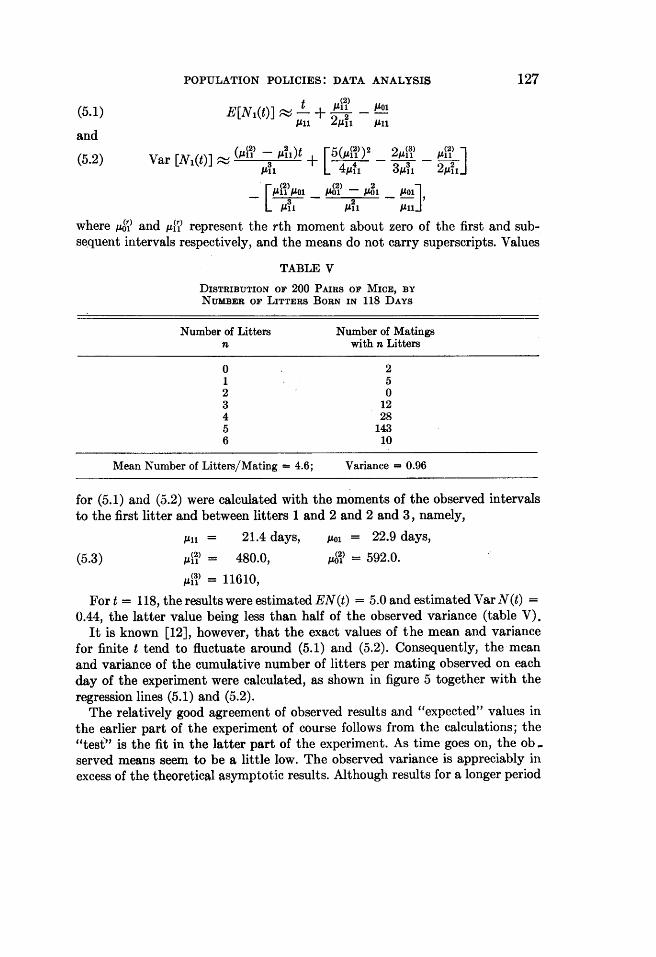
The number of litters born to 200 pairs of mice mated for 118 days undercontrolled conditions [45] is shown in table V. It was desired to examine thehypothesis that the observed variation in number of litters and in intervalsbetween litters could arise in a group of mice with equal fecundity, against analternative of varying fecundity, the term including all biological functions thataffect the process. Given a renewal process for a homogeneous group of matings,asymptotic values for the mean and variance of the number of litters expectedin t days are given by the expressions [46]


(5.1) E[Nl(t)] t t + A -PlP11 2P Mn

and

(5.2) Var [N1(t)] ( + [5(124))2 _ 2p>P _ p) ]p1h 4pefi 3 11 2A1iAfpP01 __ I2)- 2 ll

L 3I All]where p'Sl) and Alf2 represent the rth moment about zero of the first and sub-sequent intervals respectively, and the means do not carry superscripts. Values

TABLE V

DISTRIBUTION OF 200 PAIRS OF MICE, BYNUMBER OF LITTERS BORN IN 118 DAYS

Number of Litters Number of Matingsn with n Litters

0 21 52 03 124 285 1436 10

Mean Number of Litters/Mating = 4.6; Variance = 0.96

for (5.1) and (5.2) were calculated with the moments of the observed intervalsto the first litter and between litters 1 and 2 and 2 and 3, namely,

P11 = 21.4 days, P0A = 22.9 days,

(5.3) (2A' - 480.0, AWj) = 592.0.

Ai3P = 11610,For t = 118, the results were estimated EN(t) = 5.0 and estimated Var N(t) =

0.44, the latter value being less than half of the observed variance (table V).It is known [12], however, that the exact values of the mean and variance

for finite t tend to fluctuate around (5.1) and (5.2). Consequently, the meanand variance of the cumulative number of litters per mating observed on eachday of the experiment were calculated, as shown in figure 5 together with theregression lines (5.1) and (5.2).The relatively good agreement of observed results and "expected" values in

the earlier part of the experiment of course follows from the calculations; the"test"' is the fit in the latter part of the experiment. As time goes on, the ob -

served means seem to be a little low. The observed variance is appreciably inexcess of the theoretical asymptotic results. Although results for a longer period


5.000

- 4.5000(f)

~ ~~4.000

3.500 JMean U

-3 000 0,, .950 -

2.500 m.850

- 2.000z.750 - Z

-1.500<

0 .650 w1 1.000 3

Li .550CD- .500

450-

D~~ ~ ~ ~ ~~A

z 0uF .3500L M.250 - Variancez .150-

~ 050L10 20 30 40 50 60 70 80 90 100 110 120

DAYS

FIGURE 5

Mean and variance of the cumulative number of litters per matingcompared with their estimated values from (5.1) and (5.2).

would be desirable, the data suggest that the hypothesis of a homogeneous,stationary process should be rejected. It should, however, be noted that theappropriateness of the values (5.3) may be questioned, since they are based ononly 198 first intervals and 193 second intervals. A possible alternative is anal-ysis of the subgroup of matings formed by discarding the seven who had fewerthan three litters, using the distributions of their intervals. This analysis doesyield a better fit, as reported elsewhere [47]. The exact distribution of N(t) fort = 1, 2, - * -, 118, on similar assumptions is also being investigated.

In general, this preliminary analysis would seem to indicate that:(a) though it may be possible to derive an impression about the suitability

of these models for a specific set of data, improved methods of examining sucha hypothesis are needed;

(b) in this group of 200 pairs of mice, which come from a random ,mating


stock derived from the cross of four inbred lines, the evidence raises doubtsabout the existence of a homogeneous stationary process.

6. Conception delays in a heterogeneous human population

6.1. The data. The skepticism already expressed about the suitability of theassumptions in homogeneous stationary models for human reproductive datasuggests a first approach to only part of the process. Consequently, we will hereconfine ourselves to data on conception delays [14]. Such data are importantin their own right, since they provide a means for studying fecundability,whether natural or as affected by contraceptives [29].

It is customary, with some substantive justification, to assume, as was donein section 4, that, within a homogeneous population, the conception delay (X)is distributed geometrically, that is, X(x) = p(l - p)x. Available evidence, how-ever, raises doubts about the assumption of homogeneity, not only for womenusing contraceptives, but even for apparently noncontracepting women. Forexample, the data in table VI refer to 342 women in such a population [37],

TABLE VI

DISTRIBUTION OF ESTIMATED CONCEPTION DELAYS IN 342 WOMEN

Delay in Number of Women Number Proportion of EligibleMonths Still Eligible Conceiving Women Conceiving

0 342 103 .3011 239 53 .2222 186 43 .2313 143 27 .1894 116 30 .2595 86 9 .1056 77 12 .1567 65 9 .1388 56 6 .1079 50 8 .16010 42 10 .23811 32 5 .15612 27 2 .07413 25 6 .24014 19 1 .05315 18 1 .056

16-53 17 17 -

Mean Delay 3.75 Months; Variance = 30.47

who had a live birth at least nine months after marriage and who denied havingan intervening pregnancy. In an attempt to select a homogeneous group, womenaged above 25 years at marriage were excluded. The conception delay was es-timated by subtracting nine months from the interval between marriage andthe first live birth. The last column in table VI shows the estimated proportion


of women conceiving in each successive month, out of those still at risk. (I amindebted to Dr. Arthur G. Steinberg of Western Reserve University for thesehuman data.)Data on conception delays usually show a marked tendency for the monthly

inicidence of conceptioni amonig eligible women to decrcase with time [13], [16].Table VI does not do so unequivocally, but a suggestion of such a trend ispresent. Since a simple geometric distribution observed for t months is equiv-alent to a two state Markov chain undergoing t transitions, the hypothesis Ho:X(x) = p(l - p)x is equivalent to Ho: pij(x) = pij for i, j = 1, 2. It has beenshown that, under Ho, if the data in a Markov chain with s states are arrangedto resemble an s by t contingency table, the numbers in state i at time x beingtreated like numbers in independent samples, the statistic calculated as a contin-gency chi square is distributed asymptotically as x2 with (s - 1) (t - 1) degreesof freedom (d.f.) [48]. Further, this statistic can be broken down into singleindependent values distributed as x2 with one d.f. [49]. Using this test, Ho isrejected, at the P < .05 level on the data for months 0 and 1 in table VI.

Furthermore, since in a homogeneous geometric distribution, with a meanwaiting time (conception delay) x, the variance is expected to equal x(x + 1)[14], [38], the variance in this case would be expected to be approximately(3.75)(4.75) = 17.81, a value considerably below the observed variance of 30.47.Such findings may be due in part to the method of estimation, or to reporting

errors with respect to dates or intervening pregnanicy wastage. More important,fecundability may vary from one month to the next in one woman, even in arelatively short period, and is likely to vary between women. We shall nowexamine the consequences of this last possibility.

6.2. A model for conception delays in a heterogeneous group. Assume that themonthly probability of conceiving p is constant for each woman during theperiod of observation, but varies between women, being distributed as so(p) dp,and the conception delay X being a random variable given by the compoundgeometric distribution [50]

(6.1) X(x) = 10 pqXp(p) dp,

where q = 1 - p. It has been shown [14], that in such a distribution, theexpected "hazard rate," or monthly probability of conception for the sampleas a whole is a decreasing function of time, and maximum likelihood estimatorsof the moments of q have been derived from the numbers conceiving in successivemonths. In general, compound distributions have been studied by the methodof moments [51] which has been applied to compound negative binomial dis-tributions in [50], [52], and [53]. The moments estimated in these works are,however, moments not of q or p but of variables that correspond to q/p, thoughthe notation varies. Published results include expressions corresponding to (6.3)and (6.4) below and a discussion has been given [54] of the characteristics ofthe estimators in an analogous compound exponential distribution.


Letp be the fecundability, distributed as so(p) dp;q= 1 -p;-= qip;EYr be the expected value of the r.v. Yr and VY its variance;m[,] be the rth factorial moment of a variable;K[,] the corresponding cumulant;X the conception delay;s2 the variance of the conception delays in a sample of size n, that is,

s2= f (xi - -)/(n-1);c be the mean value of y in a sample, that is, c = Ej%l (1 - pj)/pjn;c(2) be the variance of y in a sample, defined as [Ey' - (Eyj)2/n]/n.From (6.1), the probability generating function (p.g.f.) of X is

m r1(6.2) E X(x)SZ = f p(l - qs)-1.(p) dp.

Successive differentiation of (6.2) with respect to s, and evaluation at s = 1,gives the generalized factorial moment of X, in agreement with [50] and [53], as

(6.3) M[r] = EX(X - 1) ... (X - r + 1) = r!Ey"and consequently, as in [14],

EX = Ey,

(6.4) EX2 = 2Ey2 + Ey,

VX = 2V-y + Ey(Ey + 1).

Assume that in a random sample of n women, the jth woman has parameterpj and the corresponding parameter yj = qj/pj. The observations from such asample are conception delays Xi. The moments of each Xi are as in (6.4) withEM = iy. Since the conception delays Xi are mutually independent, the p.g.f.for the sum of Xi in the sample is

n(6.5) '(s) = II pj(l - qjs)-

j=1

The factorial cumulants of the sum, obtained by successive differentiation withrespect to s of log I(s) and evaluation at s = 1 [55], are given by

n(6.6) K[7]( Xj) = (r - 1)! E ,-y

j=1

Hence, for a given sample,

(6.7) E[(E X)2] = E y2 + E 'y + (E yj)2 = n[c(2) + c + (n + l)c2].Conditional on the sample, from (6.4) and (6.7), the variance of the conceptiondelays is


(6.8) E(s2|sample) = -1 [,Ej (2y + yj) - -. (

-1 (fj)2]

2n-[I _ (Yj)] + c2 +c.

The unconditional expectation, since Ec(2) = (n -1)Vy/n and Ec2 = (Ey)2 +V-y/n, is

(6.9) E(s ) = 2E-9 + ETy - ()2 = 2Vy + Ey(Ey + 1).Accordingly, (6.10) and (6.11) provide estimators of the variance of 'y within

a sample and in the universe, as

((2) = n [82-x(x + 1)],(6.10) 2n - 1 [x +1]

V'y = [s-2 + 1)],

as in [14]. The estimators (6.10) are biased, an unbiased estimator being

(6.11) 1V*7= 2 [n + 1s2 - 2 -4-]In a homogeneous population, under the assumption of a simple geometricdistribution, the expected value of (6.11) is, of course, equal to zero.

6.3. Applications to the data. From (6.4) and (6.11) R'yi its standard erroris 3.75 +4 0.27 and V*-y = 6.37. The harmonic mean p is estimated as 1/(3.75 +1.00) = 0.211. The estimator of the arithmetic mean of p is equal to the propor-tion of women conceiving in the first month, that is, to 0.301, while the varianceof p may be estimated [14] from the proportions conceiving in the first twomonths as

(6.12) tVp = .301(1 - .301) - -53 = 0.055.342

Thus, it appears that, even for this group of women in the relatively shortperiod of observation, the data depart from a simple geometric distribution ofconception delays. Not only are both the mean conception delay and its varianceconsiderably in excess of what would be expected from the proportion conceivingin the first month, but the variance appreciably exceeds that expected in asimple geometric distribution with a mean conception delay of 3.75 months.Hence, we may expect the reproductive performance of this sample to have alower mean and greater variation than would be predicted from a geometricdistribution with parameter 0.211.More general inferences about the effects of heterogeneity on birth rates are

suggested by the fact, as indicated in equation (5.1), that the expected parityof a homogeneous group in time t is a function of the reciprocal of the meaniiiterval between successive births. Suppose that in a heterogeneous population


with varying mean intervals between successive births, the arithmetic meaninterval is q and the harmonic mean uA'. Then the average parity might beexpected to be a function of 1/,u', which is greater than 1/,u. Further investiga-tions into the effect of heterogeneity on birth rates are clearly indicated.

7. Summary and conclusions

A class of mathematical models for reproduction has been formulated for ahomogeneous cohort of women on the assumption that the process is independ-ent of age and parity. A summary is presented of these models, as developedin collaboration with E. B. Perrin. Despite simplification in the models, theresults provide a useful means of investigating the approximate magnitude ofthe changes in birth rates that may be expected to follow various patterns ofcontraceptive practice or changes in abortion rates. Hence, they may be usefulboth in the formulation of population policy and in efforts to evaluate theeffects of a specified program. Illustrations of such applications are given.The assumptions in these models are, however, believed to be too restrictive

for direct application of the results to human data. An attempt is presented tofit a similar model to reproductive data from a simpler organism, the laboratorymouse (from experiments performed in collaboration with D. P. Doolittle andM. New). While the test is not definitive, the results suggest that the reproduc-tive performance of this sample of a random mating stock of mice derived froma cross of four inbred lines does not conform to a stationary homogeneous process.Another set of data presented consist of the estimated conception delays to

first conception in 342 noncontracepting women (data obtained through thecourtesy of A. G. Steinberg). It seems clear that an assumption that all thesewomen have the same constant monthly probability of conception is untenable.A model is presented for the distribution of conception delays in a group wherethis probability remains constant for any women but varies between women inan unspecified manner, and the moments of the underlying distribution areestimated.

In summary, models for which explicit analytic solutions are at present avail-able have led to valuable insights into many questions relevant to the formula-tion and evaluation of population policy. There is a need, however, for morerealistic, less restricted models. One avenue of investigation into such moregeneral formulations lies in pursuing and extending the implications of lessrestrictive assumptions by mathematical analysis. Another method of studyingthese more general situations lies in the exploitation of computer models.

In addition to acknowledgments made in the text, I should like to thank mycolleagues Agnes Berger and Ruth Z. Gold for discussing some of these problemswith me and for their suggestions. At the University of Pittsburgh where muchof the work drawn on in this paper was done, Peter Amergis, Helen Chun andArthur le Gasse wrote computer programs, and Irene Nicholson assisted with


data analysis, and Sylvester Cureton anid Melvon Martin performed daily exam-inations on the mice.

REFERENCES

[1] C. GINI, "Premieres recherches sur la fecondabilit6 de la femme," Proceedings of theInternational Mathematics Congress, Toronto, 1942, pp. 889-892.

[2] R. PEARL, "Factors in human fertility and their statistical evaluation," Lancet, Vol. 225(1933), pp. 607-611.

[3] L. HENRY, "Fondements theoriques ses mesures de la f6condit6 naturelle," Rev. Inst.Internat. Statist., Vol. 21 (1953), pp. 135-151.

[4] V. M. DANDEKAR, "Certain modified forms of binomial and Poisson distributions,"Sankhyd, Vol. 15 (1955), pp. 237-250.

[5] L. HENRY, "F6condit6 et famille, modeles math6matiques," Population, Vol. 12 (1957),pp. 413-444; Vol. 16 (1961), pp. 27-48 and pp. 261-282.

[6] R. G. POTTER, JR., "Length of the observation period as a factor affecting the contra-ceptive failure rate," Milbank Memorial Fund Quarterly, Vol. 38 (1960), pp. 140-152.

[7] C. TIETZE, "Pregnancy rates and birth rates," Population Studies, Vol. 16 (1962), pp.31-37.

[8] R. G. POTTER and C. TIETZE, "A statistical model of the rhythm method," EmergingTechniques in Population Research, Proceedings of the 1962 Annual Conference, MilbankMemorial Fund, pp. 141-158.

[9] E. B. PERRIN and M. C. SHEPs, "Stochastic models for human fertility," Biometrics,Vol. 18 (1962), p. 624 (abstract).

[10] M. C. SEmPs and E. B. PERRIN, "Changes in birth rates as a function of contraceptiveeffectiveness: some applications of a stochastic model," Amer. J. Pub. Health, Vol. 53(1963), pp. 1031-1046.

[11] R. G. POTTER, "Birth intervals: structure and change," Population Studies, Vol. 17(1963), pp. 155-166.

[12] E. B. PERRIN and M. C. SHEPs, "Human reproduction: a stochastic process," Biometrics,Vol. 20 (1964), pp. 28-45.

[13] R. G. POTTER and M. P. PARKER, "Predicting the time required to conceive," PopulationStudies, Vol. 18 (1964), pp. 99-116.

[14] M. C. SHEps, "On the time required for conception," Population Studies, Vol. 18 (1964),pp. 85-97.

[15] L. HENRY, "Mesure du temps mort en fecondit6 naturelle," Population, Vol. 19 (1964),pp. 485-514.

[16] L. HENRY, "Mortalite intra-uterine et f6condabilit6," Population, Vol. 19 (1964), pp.899-940.

[17] S. W. DHARMADHIKARI, "A generalization of a stochastic model considered by V. M.Dandekar," Sankhya, Ser. A, Vol. 26 (1964), pp. 31-38.

[18] S. N. SINGH, "A probability model for couple fertility," Sankhyd, Ser. B, Vol. 26 (1964),pp. 89-94.

[19] , "On the time of first birth," Sankhyai, Ser. B, Vol. 26 (1964), pp. 95-102.[20] J. BOURGEOIS-PICHAT, "Les facteurs de la fecondit6 non dirigee," Population, Vol. 20

(1965), pp. 383-424.[21] M. SEKLANI, "Efficacite de la contraception: m6thodes et r6sultats," Population, Vol. 18

(1963), pp. 329-348.[22] D. D. JOSHI, "Stochastic models utilized in demography," United Nations World Popu-

lation Conference, Belgrade, 1965 (processed).[23] M. C. SHEPS, "Applications of probability models to the study of patterns of human


reproduction," Public Health and Population Change: Current Research Issues (edited byM. C. Sheps and J. C. Ridley), Pittsburg, University of Pittsburg Press, 1965, pp. 307-332.

[24] D. V. GLASS and D. E. C. EVERSLEY, Population in History, Chicago, Aldine, 1965.[25] M. C. SHEPS and J. C. RIDLEY (eds.), Public Health and Population Change: Current

Research Issues, Pittsburg, University of Pittsburg Press, 1965.[26] K. DAVIS and J. BLAKE, "Social structure and fertility: an analytic framework," Eco-

nomic Development and Cultural Change, Vol. 4, 1956, pp. 211-238.[27] N. B. RYDER, "Fertility," The Study of Population (edited by P. M. Hauser and 0. D.

Duncan), Chicago, University of Chicago Press, 1959, pp. 400-436.[28] C. V. KISER (ed.), Research in Family Planning, Princeton, Princeton University Press,

1962.[29] M. C. SHEps, "On the person years concept in epidemiology and demography," Milbank

Memorial Fund Quarterly, Vol. 44 (1966), pp. 69-91.[30] L. B. AREY, Developmental Anatomy, Philadelphia, Saunders, 1954 (6th ed.).[31] P. VINCENT, "Donnees biometriques sur la conception et la grossesse," Population,

Vol. 11 (1956), pp. 59-85.[32] M. C. SHEps, "Pregnancy wastage as a factor in the analysis of fertility data," Demog-

raphy, Vol. 1 (1964), pp. 111-118.[33] M. C. SHEPs and E. B. PERRIN, "The distribution of birth intervals under a class of

stochastic fertility models," Population Studies, Vol. 17 (1964), pp. 321-331.[34] I. C. UDESKY, "Ovulation in lactating women," Amer. J. Obstet. Gynec., Vol. 59 (1950),

pp. 843-851.[35] A. F. GUTTMACHER, "Fertility of man," Fertility and Sterility, Vol. 3 (1952), pp. 281-287.[36] R. G. POTTER, J. E. GORDON, M. PARKER, and J. B. Wyon, "A case study of birth

interval dynamics," Population Studies, Vol. 19 (1965), pp. 81-96.[37] M. C. Simps, "An analysis of reproductive patterns in an American isolate," Population

Studies, Vol. 19 (1965), pp. 65-80.[38] W. FELLER, An Introduction to Probability Theory and Its Applications, New York,

Wiley, 1957 (2nd ed.).[39] J. NEYMAN, "On the problem of estimating the number of schools of fish," Univ. Cali-

fornia Publ. Statist., Vol. 1 (1949), pp. 21-36.[40] W. L. SMITH, "Renewal theory and its ramifications," J. Roy. Statist. Soc. Ser. B, Vol. 20

(1958), pp. 243-302.[41] R. PYK.E, "Markov renewal processes: definitions and preliminary properties," Ann.

Math. Statist., Vol. 32 (1961), pp. 1231-1242.[42] , "Markov renewal processes with finitely many states," Ann. Math. Statist.,

Vol. 32 (1961), pp. 1243-1259.[43] M. C. SBmPs and E. B. PERRIN, "Further results from a human fertility model which

permits a variety of pregnancy outcomes," Human Biology, Vol. 38 (1966), pp. 180-193.[44] R. G. POTTER, JR., "Some physical correlates of fertility control in the United States,"

International Population Union Conference, New York, 1961, Vol. 1, London, Inter-national Population Union, 1963, pp. 106-116.

[45] D. P. DOOIrTTLE, M. NEW, and M. C. SHEPs, "Biological determinants of birth intervalsin mice," Fertility and Sterility, Vol. 18 (1967).

[46] V. K. MuRTHY, "On general renewal process," Mimeograph Series No. 293, Institute ofStatistics, University of North Carolina, 1961 (processed).

[47] M. C. SHEPS, M. NEW, and D. P. DOOLITTLE, "Mammalian reproductive data fitted toa mathematical model," to be published.

[48] T. W. ANDERSON and L. A. GOODMAN, "Statistical inference about Markov chains,"Ann. Math. Statist., Vol. 28 (1957), pp. 89-110.

[49] R. Z. GOLD, "Tests auxiliary to x2 tests in a Markov chain," Ann. Math. Statist., Vol. 34(1963), pp. 56-74.


[50] F. J. ANSCOMBE, "Sampling theory of the negative binomial logarithmic series distribu-tions," Biometrika, Vol. 37 (1950), pp. 358-382.

[51] E. J. GUMBEL, "La dissection d'une r6partition," Ann. Univ. Lyon Sect. A, Series 3,Fascicule 2 (1940), pp. 39-51.

[52] P. R. RIDER, "Estimating the parameters of mixed Poisson, binomial and Weibull dis-tributions," Bull. Inst. Internat. Statist., Vol. 39 (1961), pp. 225-232.

[53] J. E. MOSIMANN, "On the compound negative multinomial distribution and correlationsamong inversely sampled pollen counts," Biometrika, Vol. 50 (1963), pp. 47-54.

[54] P. R. RIDER, "The method of moments applied to a mixture of two exponential distri-butions," Ann. Math. Statist., Vol. 32 (1961), pp. 142-147.

[55] C. G. KEIATRi and I. R. PATEL, "Three classes of univariate discrete distributions,"Biometrics, Vol. 17 (1961), pp. 567-575.

[56] E. B. PERRIN, "Uses of stochastic models in the evaluation of population policies. II.Extension of the results by computer simulation," Proceedings of the Fifth BerkeleySymposium on Mathematical Statistics and Probability, Berkeley and Los Angeles, Uni-versity of California Press, 1966, Vol. 4, pp. 137-148.

Documents

STOCHASTIC MODELS IN THE EVALUATION OF POPULATION …