DPRIETI Discussion Paper Series 13-E-039

Stochastic Macro-equilibrium and Microfoundationsfor Keynesian Economics

YOSHIKAWA HiroshiRIETI

The Research Institute of Economy, Trade and Industryhttp://www.rieti.go.jp/en/

1

RIETI Discussion Paper Series 13-E-039

May 2013

Stochastic Macro-equilibrium and

Microfoundations for Keynesian Economics ∗

YOSHIKAWA Hiroshi University of Tokyo

Research Institute of Economy, Trade and Industry

Abstract In place of the standard search equilibrium, this paper presents an alternative concept of stochastic macro-equilibrium based on the principle of statistical physics. This concept of equilibrium is motivated by unspecifiable differences in economic agents and the presence of all kinds of micro shocks in the macroeconomy. Our model mimics the empirically observed distribution of labor productivity. The distribution of productivity resulting from the matching of workers and firms depends crucially on aggregate demand. When aggregate demand rises, more workers are employed by firms with higher productivity while, at the same time, the unemployment rate declines. The model provides a micro-foundation for Keynes’ principle of effective demand. Keywords: Labor search theory, Microeconomic foundations, Stochastic macro-equilibrium,

Unemployment, Productivity, Keynes’ principle of effective demand JRL: D39, E10, J64

∗ This work is supported by the Research Institute of Economy, Trade and Industry and the Program for Promoting Methodological Innovation in Humanities and Social Sciences by Cross-Disciplinary Fusing of the Japan Society for the Promotion of Science. The empirical works and simulation presented in the paper were carried out by Professor Hiroshi Iyetomi and Mr. Yoshiyuki Arata. The author is grateful to them for their assistance. He is also grateful for helpful comments and suggestions by Professor Masahiro Fujita and seminar participants at RIETI. He is indebted to CRD Association for the Credit Risk Database used.

RIETI Discussion Papers Series aims at widely disseminating research results in the form of professional

papers, thereby stimulating lively discussion. The views expressed in the papers are solely those of the

author(s), and do not represent those of the Research Institute of Economy, Trade and Industry.

2

1. Introduction The purpose of this paper is to present a new concept of stochastic

macro-equilibrium which provides a micro-foundation for the Keynesian theory of effective demand. Our problem is cyclical changes in effective utilization of labor. The concept of stochastic macro-equilibrium is meant to clarify the microeconomic picture underneath the Keynesian problem of aggregate demand deficiency. It is similar to standard search equilibrium in spirit, but it is based on the method of statistical physics.

The textbook interpretation of Keynesian economics originating with Modigliani (1944), regards it as economics of inflexible prices/wages. If price and wages were flexible enough, the economy would be led to the Pareto optimal neoclassical equilibrium. However, whatever the reason, when prices and wages are inflexible, the economy may fall into equilibrium with unemployment. Keynesian economics is meant to analyze such economy. In this frame of thoughts, micro-foundations for Keynesian economics would be to provide reasonable explanations for inflexible prices and wages. Toward this goal, a number of researches were done summarized under the heading of “New Keynesian economics” (Mankiw and Romer (1991)). The crux of these studies is to consider optimizing behaviors of the representative household and firm which are compatible with inflexible prices and wages. New Keynesian dynamic stochastic general equilibrium (DSGE) models are built in the same spirit.

A different interpretation of Keynesian economics was advanced by Tobin (1993).

“The central Keynesian proposition is not nominal price rigidity but the principle of effective demand (Keynes, 1936, Ch. 3). In the absence of instantaneous and complete market clearing, output and employment are frequently constrained by aggregate demand. In these excess-supply regimes, agents’ demands are limited by their inability to sell as much as they would like at prevailing prices. Any failure of price adjustments to keep markets cleared opens the door for quantities to determine quantities, for example real national income to determine consumption demand, as described in Keynes’ multiplier calculus. …

In Keynesian business cycle theory, the shocks generating fluctuations are generally shifts in real aggregate demand for goods and services, notably in capital investment.(Tobin, 1993)” Tobin dubbed his own position an “Old Keynesian view”. Certainly, the main

message of Keynes (1936) is that real demand rather than factor endowment and technology determines the level of aggregate production in the short-run simply because the rate of utilization of production factors such as labor and capital endogenously changes responding to changes in real demand. Keynes maintained that this proposition holds true regardless of flexibility of prices and wages; he, in fact, argued that a fall of prices and wages would aggravate, not alleviate the problems facing the economy in

3

deep recessions. Following Tobin, let us call this proposition the Old Keynesian view. According to

the Old Keynesian view, changes in real aggregate demand for goods and services generate fluctuations of output. The challenge is then to clarify the market mechanism by which production factors are reallocated in such a way that total output follows changes in real aggregate demand. A decrease of aggregate output is necessarily accompanied by lower utilization of production factors, and vice versa. Since the days of Keynes, economists have taken unemployment as a most important sign of possible under-utilization of labor. However, unemployment is by definition job search, a kind of economic activity of worker, and as such calls for explanation. Besides, unemployment is only a partial indicator of under-utilization of labor in the macroeconomy. The celebrated Okun’s law which relates the unemployment rate to the growth rate of real GDP demonstrates the significance of under-utilization of employed labor other than unemployment1. Without minimizing the importance of unemployment, in this paper, we focus on productivity dispersion in the economy.

To consider Keynes’ principle of effective demand, we must obviously depart from the Walrasian general equilibrium as represented by Arrow and Debreu (1954). The most successful example of “non-Walraian economics” which analyzes labor market in depth is equilibrium search theory surveyed by its pioneers Rogerson, Shimer, and Wright (2005), Diamond (2011), Mortensen (2011), and Pissarides (2000, 2011). Search theory stems from realizing limitations of the Walrasian equilibrium. The standard general equilibrium abstracts itself altogether from the search and matching costs which are always present in the actual markets. By explicitly exploring search frictions, search theory has succeeded in shedding much light on the workings of labor market.

While acknowledging the achievement of equilibrium search theory, we find several fundamental problems with the standard theory. In particular, the theory fails to provide a useful framework for explaining cyclical changes in effective utilization of labor in the macroeconomy; Shimer (2005) demonstrates that the standard search theory fails to account for stylized empirical facts on cyclical fluctuations of unemployment and vacancy.

This paper presents an alternative concept of stochastic equilibrium of the

1 Okun (1963) found that a decline of the unemployment rate by one percent raises the growth rate of real GDP by three percent. The Okun coefficient three is much larger than the elasticity of output with respect to labor which is supposed to be equal to the labor share, and, therefore, roughly one third. This finding demonstrates that there exists significant under-employment of labor other than unemployment in the macroeconomy: See Okun(1973).

4

macroeconomy based on the basic method of statistical physics. Section 2 points out limitations of standard search theory. After brief explanation of the concept of equilibrium based on statistical physics in Section 3, Section 4 presents a model of stochastic macro-equilibrium. Section 5 then explains that the stochastic macro-equilibrium provides a micro-foundation for Keynes’ principle of effective demand. It also presents suggestive evidence supporting the model. The final section offers brief concluding remarks.

2. Limitations of Search Theory

The search theory starts with the presence of various frictions and accompanying matching costs in market transactions. Once we recognize these problems, we are led to heterogeneity of economic agents and multiple outcomes in equilibrium. In the simplest retail market, for example, with search cost, it would be possible to obtain high and low (more generally multiple) prices for the same good or service in equilibrium. This break with the law of one price is certainly a big step toward reality. Frictions and matching costs are particularly significant in labor market. And the analysis of labor market has direst implications for macroeconomics. In what follows, we will discuss labor search theory.

In search equilibrium, potentially similar workers and firms experience different economic outcomes. For example, some workers are employed while others are unemployed. In this way, search theory well recognizes, even emphasizes heterogeneity of workers and firms. Despite this recognition, when it comes to model behavior of economic agent such as worker and firm, it, in effect, presumes the representative agent in the sense that stochastic economic environment is common to all the agents; Workers and firms differ only in terms of the realizations of stochastic variable of interest whose probability distribution is common. Specifically, it is routinely assumed that the job arrival rate, the job separation rate, and the probability distribution of wages are common to all the workers and firms. In some models such as Burdett and Mortensen (1998), the arrival rate is assumed to depend on a worker’s current state, namely either employed or unemployed. However, within each group, the job arrival rate is common to all the workers.

The job separation includes layoffs as well as voluntary quits. It makes absolutely no sense that all the firms and workers face the same job separation rate, particularly the probability of layoffs. White collar and blue collar workers face different risks of layoff. Everybody knows the difference between new expanding industry and old declining industry. In any case, the probability of layoffs depends crucially on the state of demand

5

for the firm’s product, and as a result, among other things, on industry and region, and ultimately the firm’s performance in the product market. The probability of layoffs certainly differs significantly across firms.

We can always calculate the average job arrived rate and job separation rate, of course. However, the average job arrival rate and the economy wide wage distribution which by definition determine the average duration of an unemployment spell would be relevant only to decisions made by say, the department of labor. When individual private economic agent makes decisions, they are not relevant because the job arrival rate, the job separation rate, and the wage distribution facing individual worker and firm are all different. Beyond that, the job arrival rate and the wage distribution cannot be independent in reality. Such complexity of actual labor market motivates our concept of stochastic macro-equilibrium.

The unrealistic assumption that they are independent and common to all the economic agents leads to an untenable consequence, that the reservation wage R is the same for all the workers in the standard search model of unemployment.

On these assumptions, the standard analysis typically goes as follows. In the equilibrium labor market, we must obtain

)1( usfu −= (1) where u is the unemployment rate, and s and f are the separation rate and the job finding rate, respectively. Equation (1) makes sure the balance between in- and out-flows of the unemployment pool. If λ is the offer arrival rate and )(wF is the cumulative distribution function of wage offers, the job finding rate f is ))(1( RFf −= λ . (2)

From equations (1) and (2), we obtain

))(1( RFs

su−+

=λ

. (3)

Equation (2), the standard equation in the literature, presumes that the offer arrival rateλ , the reservation wage R , and the cumulative distribution function of wage offers F are common to all the workers. However, as we argued above, it is obvious that in reality, λ , R and )(wF differ significantly across workers. It is actually difficult to imagine that workers of different educational attainments face the same probability distribution of wage offers; it is plainly unrealistic to assume that a youngster working at gas station faces the same probability of getting a job offer from bank as a graduate of business school. And yet, in standard search models, the assumption that )(wF is common to all the workers is routinely made, and the common )(wF is put into the Bellman equations describing behaviors of firms and workers. )(wF for the i-th

6

worker must be )(wFi . Besides, although wages are one of the most important elements in any job offer,

workers care not only wages but other factors such as job quality, tenure, and location. Preferences for these other factors which define a job offer certainly differ widely across workers, and are constantly changing over time. Rogerson, Shimer and Wright (2005; P.962) say that “although we refer to w as the wage, more generally it could capture some measure of the desirability of the job, depending on benefits, location, prestige, etc.” However, this is an illegitimate proposition. All the complexities they refer to simply strengthens the case that we cannot assume that the probability distribution of wage )(wF is common to all the workers. In fact, wage may be even a lexicographically inferior variable to some workers. For example, pregnant female worker might prefer a job closer to her home at the expense of lower wage. Workers and firms all act in their own different universes.

The second problem of standard search model pertains to the behavior of firm. It is assumed that the product market is perfectly competitive. The price is constant, and individual demand curve facing the firm is flat. It is curious that the standard search theory makes so much effort to consider the determination of wages within the firm while at the same time it leaves the price unexplained under the assumption of perfect competition. Most firms regard the determination of the prices of their own products as important as (possibly more important than) the determination of wages.

Under the assumption of perfect competition in the product market, given firm’s wage offer, whenever a worker comes, the firm is ready to hire him/her though the worker could turn down the offer. The level of employment is determined only by the number of successful matching. In Burdett and Mortensen (1998), for example, the flow of revenue generated by employed worker, p is constant and a firm’s steady-state profit given the wage offer w is simply lwp )( − where l is the number of workers of this firm.

This analytical framework leads us to some awkward conclusion. Postel-Vinay and Robin (2002), for example, interpret the empirically observed decreasing number of workers at high productivity job sites as a consequence of less recruitment efforts made by high productivity firms than by low productivity firms. However, there is no reasonable reason why high productivity firms make less recruitment efforts. A much more plausible reason is that firms are demand constrained in the product market, and that demand for goods and services produced by high productivity firm is limited.

Shimer (2005) also demonstrates that in the standard search model, an increase in the job separation rate raises both the unemployment and vacancy rates. This analytical

7

result is in stark contradiction to the well-known negative relationship between two rates, the Beveridge curve. The awkward result is obtained because the standard model assumes perfect competition in the product market, and considers strategic behavior of firms under such assumption. In the economy constrained by real demand, an increase in the job separation rate is likely to be generated by an increase in layoff which in turn, is caused by a fall of aggregate demand. The unemployment rate rises while firms laying off workers certainly post less vacancy signs.

From our perspective, the most serious problem with standard search theory is the assumption that the product market is perfectly competitive simply because the firm’s demand for labor depends crucially on the demand for the firm’s products. The assumption is particularly ill-suited for studying cyclical changes in effective utilization of labor. In this paper, following Negishi (1979), we assume that instead firms are monopolistically competitive in the sense that they face downward sloping individual demand curve in the product market.

Although the most important factor constraining the firm’s demand for labor is demand constraint in the product market, it is absolutely impossible for us to know individual demand curve facing each firm. The standard assumption in theoretical models of imperfectly competitive markets is that the demand system is symmetric, namely that firms face the same demand condition in equilibrium; See, for example, Asplund and Nocke (2006). This assumption might be justified in some cases for the analysis of an industry or a local market, but is absolutely untenable for the purpose of studying the macroeconomy. Demand is far from symmetric across firms, and there is no knowing how asymmetric it is in the economy as a whole. Our approach is based on this fact.

In summary, standard search models are built on several unrealistic assumptions. First, the job arrival rate, the job separation rate, and the probability distribution of wages are common to all the workers and firms. Some models assume that workers and firms are different in terms of their ability, preferences, and productivity (Burdett and Mortensen (1998), Postel-Vinay and Robin (2002)). However, the probability distributions of those characteristics are assumed to be utilized by all the economic agents in common.

We can always find the distribution of any variable of interest for the economy as a whole. The point is that such macro distribution is not relevant to the decisions made by individual economic agent because the “universe” of each economic agent is all different and keeps changing. In this sense, the macroeconomy is fundamentally different from a local retail market. In the case of a local retail market, one may

8

reasonably assume that all the consumers in the small region share the same distribution of prices. However, this assumption is untenable for the economy as a whole. Each agent acts in his/her own universe. For example, a worker may suffer from illness. This amounts to shocks to his utility function on one hand and to his resource constraint or “ability” on the other. His preference for job including the reservation wage, the location and working hours, necessarily changes. At the same time, the job arrival rate and the wage distribution relevant for his decision making also changes; the corresponding economy-wide information is not relevant. Note that these micro shocks are not to cancel out each other in the nature of the case. In fact, it is frictions and uncertainty emphasized by equilibrium search theory that makes the economy-wide information such as the average job arrival rate and the wage distribution is irrelevant to individual economic agent. Thus, among other things, the job arrival rate, the job separation rate, and the wage distribution are different across workers and firms.

Secondly, the standard assumption that firms are perfectly competitive without any demand constraint in the product market is particularly ill-suited for the analysis of cyclical changes in under-utilization of labor. We must assume that instead firms face downward-slowing demand curve. Because we analyze the macroeconomy, we cannot assume that demand is symmetric across firms, and moreover, we never know the details of demand constraints facing firms.

The point is not that we must explicitly introduce all the complexities characterizing labor market into analytical model. It would simply make model intractable. Rather, we must fully recognize that it is absolutely impossible to trace the microeconomic behaviors, namely decision makings of workers and firms in detail. In the labor market, microeconomic shocks are indeed unspecifiable.

Thus, for the purpose of the analysis of the macroeconomy, sophisticated optimization exercises based on representative agent assumptions do not make much sense (Aoki and Yoshikawa (2007)). This is actually partly recognized by search theorists themselves. The recognition has led them to introduce the “matching function” into the analysis. The matching function relates the rate of meetings of job seekers and firms to the numbers of the unemployed and job vacancies. The idea behind it is explained by Pissarides (2011) as follows.

“Although there were many attempts to derive an equilibrium wage

distribution for markets with search frictions, I took a different approach to labor market equilibrium that could be better described by the term “matching”. The idea is that the job search underlying unemployment in the official definitions is not about looking for a good wage, but about looking for a good job match. Moreover, it is not only the worker who is concerned to find a good match, with the firm passively prepared to hire anyone who

9

accepts its wage offer, but the firm is also as concerned with locating a good match before hiring someone.

The foundation for this idea is that each worker has many distinct features, which make her suitable for different kinds of jobs. Job requirements vary across firms too, and employers are not indifferent about the type of worker that they hire, whatever the wage. The process of matching workers to jobs takes time, irrespective of the wage offered by each job. A process whereby both workers and firms search for each other and jointly either accept or reject the match seemed to be closer to reality.

…… It allowed one to study equilibrium models that could incorporate real-world features like differences across workers and jobs, and differences in the institutional structure of labor markets.

The step from a theory of search based on the acceptance of a wage offer to one based on a good match is small but has far-reaching implications for the modeling of the labor market. The reason is that in the case of searching for a good match we can bring in the matching function as a description of the choices available to the worker. The matching function captures many features of frictions in labor markets that are not made explicit. It is a black box, as Barbara Petrongolo and I called it in our 2001 survey, in the same sense that the production function is a black box of technology. (Pissarides, 2011; pp.1093-1094)”

What job seeker is looking for is not simply a good wage, but a good job offer which cannot be uniquely defined but differs significantly across workers. It is simply unspecifiable. Pissarides recognizes such “real-world features” as differences across workers and jobs; the “universe” differs across workers and firms. Then, at the same time, he recognizes that we need a macro black box. The matching function is certainly a black box not explicitly derived from micro optimization exercises, and is, in fact, not a function of any economic variable which directly affects the decisions of individual workers and firms. Good in spirit, but the matching function is still only a half way in our view.

The matching function is based on a kind of common sense in that the number of job matchings would increase when there are a greater number of both job seekers and vacancies. However, it still abstracts itself from an important aspect of reality. As Okun (1973) emphasizes, the problem of unemployment cannot be reduced only to numbers.

“The evidence presented above confirms that a high-pressure economy

generates not only more jobs than does a slack economy, but also a different pattern of employment. It suggests that, in a weak labor market, a poor job is often the best job available, superior at least to the alternative of no job. A high-pressure economy provides people with a chance to climb ladders to better jobs.

The industry shifts are only one dimension of ladder climbing. Increased upward movements within firms and within industries, and greater geographical flows from lower-income to higher-income regions, are also likely to be significant. (Okun, 1973; pp.234-235)”

Dynamics of unemployment cannot be separated from qualities of jobs, or more

10

specifically distribution of productivity on which we focus in the present paper. Our analysis, in fact, demonstrates that the matching “function” is not a

structurally given function even in the short-run, but depends crucially on the level of aggregate demand. To explicitly consider these problems, we face greater complexity and, therefore, need a “greater macro black box” than the standard matching function. This is the motive for stochastic macro-equilibrium we explain in the next section.

3. Stochastic Macro-equilibrium —— The Basic Idea

Our vision of the macroeconomy is basically the same as standard search theory. Workers are always interested in better job opportunities, and occasionally change their jobs. Job opportunities facing workers are stochastic depending on vacancy signs posted by firms. Firms, on the other hand, make their efforts to recruit and retain the best workers for their purposes. We assume that firms are demand-constrained in the product market. Demand determines the level of production and, as a consequence, demand for labor.

Unemployment, a great challenge to any economy, deserves special attention in economic analysis, but actually a significant part of workers change their jobs without experiencing any spell of unemployment. The importance of on the job search also means that job turnover depends crucially on the distribution of qualities of jobs in the economy. Postel-Vinay and Robin (2002), in fact, analyze on-the-job search explicitly considering workers with different abilities on one hand and firms with different productivities on the other. Their analysis, however, still depends on restrictive assumptions that all the workers face the same job offer distribution independent of their ability and employment status, and that the product market is perfectly competitive.

While workers search for suitable jobs, firms also search for suitable workers. Firm’s job offer is, of course, conditional on its economic performance. The present analysis focuses on the firm’s labor productivity. The firm’s labor productivity increases thanks to capital accumulation and technical progress or innovations. However, those job sites with high productivity remain only potential unless firms face high enough demand for their products; firms may not post job vacancy signs or even discharge the existing workers when demand is low. As noted above, we assume that firms are all monopolistically competitive in the sense that they face downward sloping individual demand curves, and the levels of production are determined by demand rather than increasing marginal costs.

Formally, a most elegant general equilibrium model of monopolistic competition

11

is given by Negishi (1960-61). Negishi (1979) persuasively argues that when the firm is monopolistically competitive, the downward-sloping individual demand curve must be kinked at the current level of output and price. The corresponding marginal revenue becomes discontinuous as shown in Figure 1. The response of the firm’s sales to a change in price is asymmetric because of different reactions on the part of vital firms. With the perceived kinked individual demand curve, a shift of demand is basically absorbed by a change in output leaving price unchanged. As Tobin (1993) says, the model opens the door for “quantities determine quantities.2”

Negishi (1979; Chapter 6) establishes the existence of general equilibrium of monopolistically competitive firms facing the kinked individual demand curve as shown in Figure 1. Though the equilibrium exists, it is indeterminate because the initial levels of the firms’ output and price (the kink point of the individual demand curve) must be exogenously given. To give such initial condition amounts to determining the level of individual demand curve facing each firm. The present analysis provides a rule for allocating the aggregate demand to monopolistically competitive firms based on the principle of statistical physics.

Negishi (1979)’s general equilibrium model of monopolistically competitive firms abstracts itself from frictions and uncertainty in the labor market. Unlike capital, worker either stays at a job, moves to another, or searches for one as the unemployed. Firms try to recruit the best workers for their purposes. These are, of course, aspects of labor market which search theory analyses. We follow its spirit, but not its analytical method.

In the present analysis, we simply assume that firms with higher productivity make more attractive job offers to workers. This assumption means that whenever possible, workers move to firms with higher productivity. However, for workers to move to firms with higher productivity, it is necessary that those firms must decide to fill the vacant job sites, and post enough number of vacancy signs. They post such vacancy signs only when they face an increase of demand for their products, and decide to raise the level of production. It also goes without saying that high productivity firms keep their existing workers only when they face high enough demand.

The question we ask is what the distribution of employed workers is across firms whose productivities differ. As we argued in the pervious section, because microeconomic shocks to both workers and firms are so complex and unspecifiable, optimization exercises based on representative agent assumptions do not help us much.

2 In Negishi (1979)’s model of monopolistically competitive firms, a change in wage does not affect the level of production, and, therefore leaves the number of vacancy unchanged because marginal revenue is discontinuous. This is in stark contrast to the standard search model.

12

In particular, we never know how the aggregate demand is distributed across monopolistically competitive firms. To repeat, among other things, the job arrival rate, the job separation rate, and the probability distribution of wages (or more generally measure of the desirability of the job) differ across workers and firms. This recognition is precisely the starting point of the fundamental method of statistical physics3. At first, one might think that allowing too large a dispersion of individual characteristics leaves so many degrees of freedom that almost anything can happen. However, it turns out that the methods of statistical physics provide us not only with qualitative results but also with quantitative predictions.

In the present model, the fundamental constraint on the economy as a whole is aggregate demand D . Accordingly, to each firm facing the downward-sloping individual demand curve, the level of demand for its product is the fundamental constraint. The problem is how the aggregate demand D is allocated to these monopolistically competitive firms. Our model provides a solution. The basic idea behind the analysis can be explained with the help of the simplest case.

Suppose that kn workers belong to firms whose productivity is

kc ( 'kk cc < where 'kk < ). There are K levels of productivity in the economy ( Kk ,,2,1 = ). The total number of workers N is given.

NnK

kk =∑

=1

(4)

A vector ),,,( 21 Knnnn = shows a particular allocation of workers across firms with different productivities. The combinatorial number nW of obtaining this allocation, n , is equal to that of throwing N balls to K different boxes. It is

!

!

1∏=

= K

kk

n

n

NW (5)

Because the number of all the possible ways to allocate N different balls to K different boxes is NK , the probability that a particular allocation ),,,( 21 Knnnn = is obtained is

!

!1

1∏=

== K

kk

NNn

n

n

NKK

WP . (6)

It is the fundamental postulate of statistical physics that the state or the allocation ),,,( 21 Knnnn = which maximizes the probability nP or (6) under macro-constraints is

3 Foley (1994), in his seminal application of this approach to general equilibrium theory, advanced the idea of “statistical equilibrium theory of markets”.

13

to be actually observed in the economy. The idea is similar to maximum likelihood in statistics/econometrics.

Maximizing nP is equivalent to maximizing nPln . Applying the Stirling formula for large number x

xxxx −≅ ln!ln , (7)

we find that the maximization of nPln is equivalent to that of S .

k

K

kk ppS ln

1∑=

−= )(Nn

p kk = (8)

S is the Shannon entropy, and captures the combinatorial aspect of the problem. It can be easily understood with the help of a simple example. When we throw a pair of dice, the possible sums range from two to twelve. Six is much more likely than twelve simply because the combinatorial number of the former is five whereas that of the latter is only one. Though the combinatorial consideration summarized in the entropy plays a decisive role for the final outcome, that is not the whole story, of course. The qualification “under macro-constraints” is crucial.

The first macro-constraint concerns the labor endowment, (4). The second macro-constraint concerns the effective demand.

DncK

kkk =∑

=1

(9)

Here, aggregate demand D is assumed to be given. In our analyis, we explicitly analyze the allocation of labor ),,,( 21 Knnn . Note, however, that the allocation of labor is basically equivalent to the allocation of the aggregate demand to monopolistically competitive firms.

To maximize entropy S under two macro-constraints (4) and (9), set up the following Lagrangean form L :

−+

−+

−= ∑∑∑

===

K

kkk

K

kk

kK

k

k ncDnNNn

Nn

L111

ln βα (10)

with two Lagrangean multipliers, α and β . Maximization of this Lagrangean form with respect to kn leads us to the first-order conditions:

kk NcN

Nn

βα −−−=

1ln ( Kk ,,2,1 = ) (11)

which are equivalent to

[ ]kk NcN

Nn

βα −−−= 1exp . (12)

14

Because Nnk sums up to one, we obtain

∑=

−

−

= K

k

Nc

Nck

k

k

e

eNn

1

β

β

(13)

Thus, the number of workers working at firms with productivity kc is exponentially distributed. It is known as the Boltzmann distribution in physics.

Here arises a crucial difference between economics and physics. In physics, kc corresponds to the level of energy. Whenever possible, particles tend to move toward the lowest energy level. To the contrary, in economics, workers always strive for better jobs offered by firms with higher productivity kc . In fact, if allowed, all the workers would move up to the job sites with the highest productivity, Kc . This situation shown in Figure 2 corresponds to the textbook Pareto optimal equilibrium with no frictions. However, this state is actually impossible unless the level of aggregate demand D is so high as equal to the maximum level NcD K=max . Only when D is equal to maxD , demand-constrained firms with the highest productivity face high enough individual demand curves so that they have incentives to employ N workers. On the part of workers, they would be able to find job sites with the highest productivity because firms with Kc try hard to keep their existing workers, and at the same time post enough vacancy signs to aggressively recruit. With frictions, D must be actually higher than

maxD for the state shown in Figure 2 to be realized. The maximum level of aggregate demand maxD is only imaginary, however.

When D is lower than maxD , the story is quite different. Some workers —— a majority of workers, in fact, must work at job sites with productivity lower than Kc . How are workers distributed over job sites with different productivity? Obviously, it depends on the level of aggregate demand. When D reaches its lowest level, minD , workers are distributed evenly across all the sectors with different levels of productivity,

Kccc ,,, 21 (Figure 3). Here, minD is defined as KcccND k /)( 21min +++= .

It is easy to see that the lower the level of D is, the greater the combinatorial number of distribution ),,,( 21 Knnn which satisfies aggregate demand constraint (9) becomes. Note that this combinatorial number basically corresponds to the distribution of demand for goods and services across job sites at monopolistically competitive firms with different levels of productivity.

As explained above, the combinatorial number nW of a particular allocation ),,,( 21 Knnnn = is basically equivalent to the Shannon entropy, S defined by (8).

S increases when D decreases. In the extreme case where D is equal to (or more realistically greater than) the maximum level maxD , all the workers work at job sites

15

with the highest productivity because whenever possible, workers move to better job sites with higher productivity (Figure 2). In this case, the entropy S becomes zero, its lowest level, because 1=NnK and )(0 KkNnk ≠= . In the other extreme where

KNnK = (Figure 3), the entropy S defined by (8) becomes Kln , its maximum level. Thus, the relation between the entropy S and the level of aggregate demand D looks like the one shown in Figure 4.

At this stage, we can recall that the Lagrangean multiplier β in (10) for aggregate demand constraint is equal to

DS

DL

∂∂

=∂∂

=β . (14)

β is the slope of the tangent of the curve as shown in Figure 4, and, therefore, is negative4. Table 1 shows how negative β relates to the level of aggregate demand D .

With negative β , the exponential distribution (13) looks like the one shown in Figure 5. Whenever possible, workers always move toward job sites with higher productivity. As a result, the distribution is upward-sloping. However, unless the aggregate demand is equal to (or greater than) the maximum level, maxD , workers’ efforts to reach job sites with the highest productivity Kc must be frustrated because firms with the highest productivity do not need to employ a large number of workers and are less aggressive in recruitment, and accordingly it gets harder for workers to find such jobs. As a consequence, workers are distributed over all the job-sites with different levels of productivity.

The maximization of entropy under the aggregate demand constraint (10), in fact, balances two forces. On one hand, whenever possible, workers are assumed to move to better jobs which are identified with job sites with higher productivity. It is the outcome of successful job matching resulting from the worker’s search and the firm’s recruitment. When the level of aggregate demand is high, this force dominates. However, when D is lower than maxD , there are in general a number of different allocations

),,,( 21 Knnn which are consistent with D . As we explained in the previous section, micro shocks facing both workers and

firms are truly unspecifiable. We simply do not know, on one hand, which firms with

4 In physics, β is positive in most cases. This difference arises because workers strive for job sites with higher productivity, not the other way round (Iyetomi (2012)). In physics, β is equal to the inverse of temperature, or more precisely, temperature is defined as the inverse of DS ∂∂ when S is the entropy and D energy. Thus, negative β means the negative temperature. It may sound odd, but the notion of negative temperature is perfectly legitimate in such systems as the one in the present analysis; see Ramsey (1965) and Appendix E of Kittel and Kroemer (1980).

16

what productivity face how much demand constraint and need to employ how many workers with what qualifications, and on the other, which workers are seeking what kind of jobs with how much productivity. Here comes the maximization of entropy. It gives us the distribution ),,,( 21 Knnn which corresponds to the maximum combinatorial number consistent with given D . The entropy maximization under aggregate demand constraint plays, therefore, the role similar to the matching function in the standard search theory. Note that unlike the standard matching function which focuses only on the number of jobs, the matching of job quality characterized by productivity plays a central role in the present analysis. The matching function presumes that the number of job matching increases when the numbers of the unemployed and vacancy increase. In the present analysis, the matching of high productivity jobs is ultimately conditioned by the level of aggregate demand because high aggregate demand loosens demand constraints facing monopolistically competitive high productivity firms, and vice versa. Uncertainty and frictions emphasized by the standard search theory are not exogenously given, but depend crucially on aggregate demand; In a booming gold-rush town, one does not waste a minute to find a good job!

The distribution of workers over job-sites with different productivity levels which results from this analysis is an upward-sloping exponential distribution as shown in Figure 5. As one should expect, the higher the level of aggregate demand D is, the steeper the distribution becomes meaning that more workers are mobilized to jobs with higher productivity (Okun (1973)).

It is essential to understand that the present approach does not regard economic agents’ behaviors as random. Certainly, firms and workers maximize their profits and utilities. The present analysis, in fact, presumes that workers always strive for better jobs characterized by higher productivity. However, firms are demand-constrained facing downward-sloping demand curves. As a result of profit-maximization, the optimal level of production is constrained by demand. Unless the level of aggregate demand is extremely high and equal to (with frictions, greater than) its maximum level

NCK , micro demand constraints become effective. In this case, the entropy matters because we can never know details of micro behaviors. Randomness underneath the entropy maximization comes from the fact that both the objective functions of and constraints facing a large number of economic agents are constantly subject to unspecifiable micro shocks. We must recall that the number of households is of order 107, and the number of firms, 106. Therefore, there is nothing for outside observers, namely economists analyzing the macroeconomy but to regard a particular allocation under macro-constraints as equi-probable. Then, it is most likely that the allocation of

17

the aggregate demand and accordingly workers which maximizes the probability nP or (6) under macro-constraints is realized5. 4. The Model

The above analysis shows that the distribution of workers at firms with different productivities depends crucially on the level of aggregate demand. Though the basic model is good enough to explain the basic idea, it is too simple to explain the empirically observed distribution of labor productivity.

Empirical Distribution of Productivity

Figures 6 (a), (b) and (c) show the distributions of workers at different productivity levels for the Japanese economy ((a) total, (b) manufacturing and (c) non-manufacturing industries). The data used are the Nikkei Economic Electric Database (NEEDS, http://www.crd-office.net/CRD/english/index.html) and the Credit Risk Database (CRD, http://www.crd-office.net/CRD/english/index.html) which cover more than a million large and medium/small firms for 2007.

The “productivity” here is simply value added of the firm divided by the number of employed workers, that is, the average labor productivity. Theoretically, we should be interested in unobserved marginal productivity, not the average productivity. Besides, proper “labor input” must be in terms of work hour, or for that matter even in terms of work efficiency units rather than the number of workers. For these reasons, the average labor productivity shown in the figure is a crude measure of theoretically meaningful unobserved marginal productivity. However, Aoyama et. al. (2010; p.38-41) demonstrates that when the average productivity and measurement errors are independent, the distribution of true marginal productivity obeys the power law with the 5 This method has been time and again successful in natural sciences when we analyze object comprising many micro elements. Economists might be still skeptical of the validity of the method in economics saying that inorganic atoms and molecules comprising gas are essentially different from optimizing economic agents. Every student of economics knows that behavior of dynamically optimizing economic agent such as the Ramey consumer is described by the Euler equation for a problem of calculus of variation. On the surface, such a sophisticated economic behavior must look remote from “mechanical” movements of an inorganic particle which only satisfy the law of motion. However, every student of physics knows that the Newtonian law of motion is actually nothing but the Euler equation for a certain variational problem; particles minimizes the energy or the Hamiltonian!. It is called the principle of least action: see Chapter 19 of Feynmann (1964)’s Lectures on Physics, Vol. II. Therefore, behavior of dynamically optimizing economic agent and motions of inorganic particle are on a par to the extent that they both satisfy the Euler equations for respective variational problems. The method of statistical physics can be usefully applied not because motions of micro units are “mechanical,” but because object under investigation comprises many micro units individual movements of which we are unable to know. It leads us to a specific exponential distribution (13).

18

same exponent as that for the measured average productivity. In other words, distribution is robust with respect to measurement errors in the present case. Incidentally, we also note that the Pareto efficiency of the economy pertains to marginal products of production factors, not to total factor productivity (TFP) some economists focus on.

Figure 6 drawn on the double logarithm plane broadly shows that (1) the distribution of labor productivity is single-peaked, (2) in the low productivity (left) region, it is upward-sloping exponential whereas (3) in the high productivity (right) region, it obeys downward-sloping power-law (Aoyama et. al., (2010)). Ikeda and Souma (2009) find a similar distribution of productivity for the U.S. while DelliGatti et. al. (2008) find power-law tails of productivity distribution for France and Italy. In what follows, we present an extended model based on the principle of statistical physics for explaining the broad shape of this empirically observed distribution.

We explained in the previous section that the entropy maximization under macro constraints leads us to exponential distribution. This distribution with negative β can explain the broad pattern of the left-hand side of the distribution shown in Figures 6 (a) (b) and (c), namely an upward-sloping exponential distribution (Iyetomi (2012)). However, we cannot explain the right-hand side downward-sloping power distribution for high productivity firms. To explain it, we need to make an additional assumption that the number of potentially available high-productivity jobs is limited, and that it decreases as the level of productivity rises.

Dynamics of Potential Job Creation/Destruction

Potential jobs are created by firms by accumulating capital and/or introducing new

technologies, particularly new products. On the other hand, they are destroyed by firms’

losing demand for their products permanently. Schumpeterian innovations by way of

creative destruction raise the levels of some potential jobs, but at the same time lower

the levels of others. In this way, the number of potential jobs with a particular level of

productivity keeps changing. They remain potential because firms do not attempt to fill

all the job sites with workers. To fill them, firms either keep the existing workers on the

job or post job vacancy signs, but it is an economic decision, and depends crucially on

the economic conditions facing the firms. The most important constraint on the firm’s

employment is the level of demand in the product market. The number of potential job

sites, therefore, is not exactly equal to, but rather imposes a ceiling on the sum of the

number of filled job sites, namely employment and the number of job openings or

19

vacancy signs.

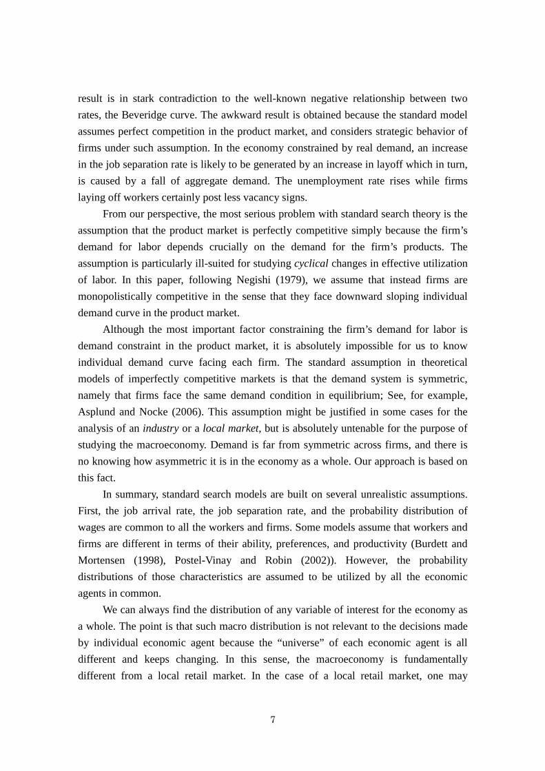
The statistical theory we will discuss later explains how employment is

determined. In this sub-section, we first consider dynamics of potential job creation and

destruction. Causes of creation/destruction of potential job sites are micro-shocks, and

as explained in the previous section, unspecifiable. The best way to describe them is

Markov model. Good examples in economics are Champernowne (1950) on income

distribution, and Ijiri and Simon (1979) on size distribution of firms. Here, we adapt the

model of Marsili and Zhang (1998) to our own purpose. The goal of the analysis is to

derive a power-law distribution such as the one for the tail of the empirically observed

distribution of labor productivity.

Suppose that there are jf ”potential” jobs with productivity, jc ( 'jj cc < ,

when 'jj < ). In small time interval dt , the level of productivity c of a potential job

site increases with probability dtcw )(+ by a small amount which we can assume is

unity without loss of generality. We denote this probability as )(cw+ because +w

depends on the level of c . Likewise, it decreases by a unit with productivity dtcw )(− .

Thus, )(cw+ and )(cw− are transition rates for the processes 1+→ cc and

1−→ cc , respectively. As noted above, the productivity of job site changes for many

reasons. It may reflect technical progress or innovations. Given significant costs of

adjusting labor, productivity also changes when demand for firm’s products change. For

example, when demand for firm’s products falls, labor productivity necessarily declines.

The decline of productivity in this case reflects labor hoarding (Fay and Medoff (1985)).

These changes are captured by transition rates, )(cw+ and )(cw− in the model.

We also assume that a new job site is born with a unit of productivity with

probability dtp . On the other hand, a job site with productivity 1=c will cease to

exist if c falls to zero. Thus the probability of exit is dtcw )1( =− . A set of the

transition rates and the entry probability specifies a jump Markov process.

Given this Markov model, the evolution of the average number of job sites of

productivity c at time t , ),( tcf , obeys the following master equation:

),1()1(),1()1(),( tcfcwtcfcwt

tcf+++−−=

∂∂

−+

1,),()(),()( cptcfcwtcfcw δ+−− −+ , (15)

Here, 1,cδ is 1 if 1=c , and 0 if otherwise. This equation shows that change in ),( tcf

20

over time is nothing but the net inflow to the state c .

We consider the steady state or the stationary solution of equation (15) such that

0/),( =∂∂ ttcf . The solution )(cf can be readily obtained by using the boundary

condition that pfw =− )1()1( :

∏−

= −

+

+−−

=1

1 )1()()1()(

c

k kcwkcwfcf . (16)

Here, we make an important assumption on the transition rates, +w and −w .

Namely, we assume that the probabilities of an increase and a decrease of productivity

depend on the current level of productivity of job site. Specifically, the higher the

current level of productivity, the larger a chance of unit productivity change. This

assumption means that the transition rates can be written as αcacw ++ =)( and αcacw −− =)( , respectively. Here, +a and −a are positive constants, and α is greater

than 1. Under this assumption, the stationary solution (16) becomes

*/)(

)(

)/)1(1(/)1(1)1()( cc

c

ecc

CfCf

fcf −−≅−

−= α

αα

α

. (17)

where

1)(

* )/)1(( −≡ αCfc and ∑∞

=

≡1

)( )(c

cfcC αα .

We use the relation )(/)1(1/ αCfaa −=−+ . The approximation in equation (17)

follows from 1/)1( )( <<αCn , and the exponential cut-off works as c approaches to *c .

However, the value of *c is practically large, and therefore, we observe the power law

distribution α−∝ ccn )( for a wide range of c in spite of the cut-off. Therefore, under

the reasonable assumption, we obtain power law distribution for job sites, jf .

The above model can be understood easily with the help of an analogy with the

formation of cities. Imagine that ),( tcf is the number of cities with population c at

time t . )(cw+ corresponds to a birth in a city with population c , or an inflow into the

city from another city. Similarly, )(cw− represents a death or an exit of a person

moving to another city. These rates are the instantaneous probabilities that the

population of a city with the current population c either increases or decreases by 1.

They are, therefore, the entry and exit rates of one person times the population c of the

city, respectively. In addition, a drifter forms his own one-person city with the

instantaneous probability p . In this model, the dynamics of ),( tcf or the average

21

number of cities with population c , is given by equation (15). In the case of population

dynamics, one might assume that the entry (or birth) and exit (or death) rates of a person,

+a and −a , are independent of the size of population of the city in which the person

lives. In that case )(cw+ and )(cw− become linear functions of c , namely ca+ and

ca− . However, even in population dynamics, one might assume that the entry rate of a

person into a large city is higher than its counterpart in a smaller one because of better

job opportunities or the social attractiveness of such places, as encapsulated in the

words of the song, “bright lights, big city”. The same may hold true for exit and death

rates because of congestion or epidemics.

In turns out that in the dynamics of productivity of job site, both the “entry” and

“exit” rates of an existing “productivity job site” are increasing functions of c , namely

the level of productivity in which that particular job site happens to be located; to be

concrete, ca+ and ca− . Thus, )(cw+ becomes ca+ times c which is equal to 2ca+ . Likewise, we obtain 2)( cacw −− = . This is the case of the so-called Zipf law (Ijiri

and Simon (1975)). Thus, under the reasonable assumption that the probability of a unit

change in productivity is an increasing function of its current level c , we obtain power

law distribution for job sites jf .

Economists often presume that changes in productivity are caused by supply-side

factors such as technical progress and entry/exit of firm alone. However, an important

source of productivity change is actually a sectoral shift of demand. Indeed, Fay and

Medoff (1985) documented such changes in firm’s labor productivity by way of changes

in the rate of labor hoarding. Stochastic productivity changes as described in our

Markov model certainly include technical progress, particularly in the case of an

increase, but at the same time they embrace allocative demand disturbances. By their

careful study of industry-level productivity and worker flows, Davis et al. (1996) found

that while job creation is higher in industries with high total factor productivity growth,

job destruction for an industry is not systematically related to productivity growth; job

destruction is actually highest in the industries in the top productivity growth quintile

(Table 3.7, Davis et. al. (1996, P.52)). This finding suggests the importance of negative

demand shocks for job destruction. Distribution of Productivity

Distribution of potential job sites with high productivity obeys downward-sloping

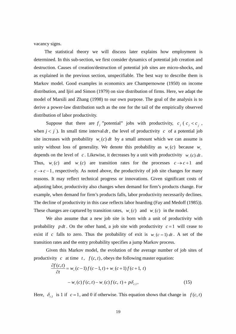
22

power law. However, the determination of employment by firms with various levels of

productivity is another matter. To fill potential job sites with workers is the firm’s

economic decision. The most important constraining factor is the level of demand

facing the firm in the product market. Whatever the level, to fill potential job sites, the

firm must either keep the existing workers on the job or post vacancy signs toward

successful job matching. Such actions of the firms and job search of workers are not

random but purposeful. However, micro shocks affecting firms and workers are just

unspecifiable. Then, how are workers actually employed at firms with various levels of

productivity? This is the problem we consider in what follows.

The number of workers working at the firms with productivity, jc , namely jn is

},,1,0{ jj fn ∈ ),2,1( Kj = . (18)

Here, jf is the number of potential jobs with productivity jc , and puts a ceiling on

jn 6. We assume that in the low productivity region, jf is large enough meaning that

jn is virtually unconstrained by jf . In contrast, in the high productivity region, jf

constrains jn , and its distribution is power distribution as we have analyzed above.

Like many others, Postel-Vinay and Robin (2002) assume that there is no ceiling

for job-sites with high productivity. On this assumption, they regard a decreasing

number of workers with high productivity jobs as a consequence of less recruitment

efforts made by high productivity firms than by low productivity firms. This is an

awkward interpretation. There is no reasonable reason why high productivity firms

make less recruitment efforts than low productivity firms. A more plausible assumption

is that firms are monopolistically competitive facing the downward-sloping individual

demand curve rather than the price takers in the product market, and that jobs with high

productivity are limited in number by such demand constraints. Suppose, for example,

that automobile industry is a high productivity industry. It would be unreasonable to

argue that the level of employment in the industry is only the outcome of job matching,

and that a limited size of employment is due to a lack of the firms’ recruitment efforts.

The size of car producers is basically determined by the level of demand for cars and

their capacity.

6 When the number of potential jobs with high productivity is limited, behavior of economic agents necessarily becomes correlated; If good jobs are taken by some workers, it becomes more difficult for others to find such jobs. Garibaldi and Scalas (2010) suggest that we study the problem by Markov model with such constraints.

23

The total number of employed workers is simply the sum of jn :

∑=

=K

jjnN

1

. (19)

In the basic model explained in section 3, the total number of employed workers, N is

exogenously given (equation (4)). In the present model, N is assumed to be variable.

N is smaller than the exogenously given total number of workers or labor

force, L ( LN < ). The difference between L and N is the number of the unemployed,

U :

NLU −= . (20)

As in the basic model, firms are monopolistically competitive facing the

downward-sloping individual demand curve, and as a consequence the total output is

constrained by the aggregate demand, D (Equation (9)). In the basic model, D is

literally given. Accordingly, total output is also given by equation (9), and is constant. In

the present model, we more realistically assume that in accordance with fluctuations of

aggregate demand, total output Y also fluctuates. Specifically, Y defined by

∑=

=K

kkk ncY

1

(21)

is now stochastic, and its expected value >< Y is equal to constant D . That is, we

have

DY >=< . (22)

Aggregate demand constrains total output in the sense of its expected value.

Under this assumption, the probability of total output Y turns out to be

exponential; The density function )(Yg is

∑ −

−

=

i

Y

Y

i

i

eeYg β

β

)( (23)

This result is obtained by the method of Gibbs’ canonical ensemble. Gibbs established the statistical mechanics by introducing the concept of “canonical ensemble” which is a collection of macro states, Y in our present case. Suppose that there are K possible levels of Y denoted by KYY ,1 . For the moment, we reinterpret kn as the number of cases where Y takes the value kY ( Kk ,,1 = ). The sum of kn , N is given. Then, kn satisfies equation (4). We assume that the average of Y is equal to constant D .

24

DNn

YK

k

kk =

∑

=1

(24)

Replacing kc by NYk / , we observe that equation (24) is equivalent to equation (9). Thus, we can apply the exactly same entropy maximization as we did in the basic model in section 3. It leads us to equation (23). In (23), β is the Lagrange multiplier for constraint (24) in the maximization of entropy (8).

Obviously, Y constrained by aggregate demand D affects the distribution of

workers, kn (equation (21)). In the present model, the number of employed workers

N is not constant, but changes causing changes in unemployment. Besides, the number

of potential job sites with high productivity, jf constrains jn . Under these

assumptions, we seek the state which maximizes the probability nP or equation (6).

Before we proceed, it is useful to explain partition function because it is rarely

used in economics, but we will use it intensively in the subsequent analysis. When a

stochastic variable Y is exponentially distributed, that is, its density function )(Yg is

given by equation (23), partition function Z is defined as

∑ −=i

YieZ β . (25)

This function is extremely useful as moment generating function. For example, the first

moment or the average of Y can be simply found by differentiating Zlog with respect

to β .

∑

∑∑ −

−

−

−−=−=−

i

Yi

Yi

i

Yi

i

i

e

eYe

dd

dZd

β

β

β

ββ

)()log(log

)()()( ii

ii

i

Y

Y

ii YEYgY

eeY

i

i

=== ∑∑∑ −

−

β

β

(26)

As in the basic model, we want to find the state which maximizes the probability,

nP or equation (6). We have two macro-constraints, equations (19) and (21). The total

number of workers employed N is, however, not constant but variable. The aggregate

output Y is also not constant but obeys the exponential distribution, namely equation

(23).

Because the level of total output depends on the total number of employed

workers N , we denote iY as )(NYi . Then, the canonical partition function NZ can

25

be written as

∑ −=i

NYN

ieZ )(β . (27)

Using equation (21), we can rewrite this partition function as follow:

{ }

)exp(1

∑ ∑=

−=in

K

iiiN ncZ β . (28)

Unfortunately, it is generally difficult to carry out the summation with respect to { }in

under constraint (19), namely ∑= inN . Rather than taking N as given, we better

allow N to be variable as we do here, and consider the grand canonical partition

functionΦ .

The grand canonical partition function is defined as

∑∞

=

=Φ0N

NN Zz (29)

where

βµez = . (30)

The parameter µ is called the chemical potential in physics, and measures the marginal

contribution in terms of energy of an additional particle to the system under

investigation. In the present model, N is the number of employed workers, and,

therefore, µ measures the marginal product of a worker who newly acquired job out

of the pool of unemployment. Thus, µ is equivalent to the reservation wage, or more

generally the “reservation job offer” of the unemployed. When µ is high, the

unemployed worker is choosy, and vice versa.

Substituting equation (28) into equation (29), the grand canonical partition

function Φ becomes as follows:

}exp{0∑ ∑∑ −=Φ

∞

= nj jjj

N

N cnz β where βµez = (31)

Using the definitions of z , (30), and also N , (19), we have

])(exp[}exp{10

)( 1jj

K

j njn jjj

N

nn nccnej

K −=−=Φ ∏∑∑ ∑∑=

∞

=

++ µβββµ . (32)

Because there is ceiling jf for jn (constraint (18)), (32) can be rewritten as follows:

26

∏∏=

−

−+−−

= −−

=++=ΦK

jc

cfcfc

K

j eeee

jj

1)(

)()1()()(

1

]1

1[]1[ µβ

µβµβµβ (33)

With this grand canonical partition functionΦ , we can easily obtain the expected value of the total number of employed workers N , >< N by differentiating Φlog with respect toµ which corresponds to the reservation wage of the unemployed worker. This can be seen by differentiating (29) and noting the definition of z , (30).

>=<=∂∂

=Φ∂∂

∑

∑∑ ∞

=

∞

=∞

=

NZe

ZNeZe

NN

N

NN

N

NN

N ][1)]log([1]log[1

0

0

0 βµ

βµ

βµβ

βµβµβ. (34)

In the present case, Φ is actually given by equation (33). Therefore, we can find >< N as follows.

]log[1Φ

∂∂

=µβ

N

)}1log()1{log(1 )()()1(

1

jjj ccfK

jee −−+

=

−−−∂∂

= ∑ µβµβ

µβ

∑=

−

−

−+

−+

−−

−

+=

K

jc

c

cf

cfj

j

j

jj

jj

ee

e

ef

1)(

)(

)()1(

)()1(

]11

)1([ µβ

µβ

µβ

µβ

(35)

The expected value of the number of workers employed on the job sites with productivity jc , >< jn is simply the corresponding term in the summation of >< N or equation (35).

11

)1()(

)(

)()1(

)()1(

−−

−

+= −

−

−+

−+

j

j

jj

jj

c

c

cf

cfj

j ee

e

efn µβ

µβ

µβ

µβ

(36)

Equation (36) determines the distribution of workers across job-sites with different levels of productivity in our stochastic macro-equilibrium.

Figure 7 shows how this model works. On one hand, there is dynamics of creation and destruction of potential job sites with various levels of productivity (Figure 7 (a)). We presented a Markov model which leads us to power-law tail of productivity distribution in the steady state. At the same time, there is another dynamics of job matching which corresponds to the standard search theory (Figure 7(b)). Convolution of two dynamics determines the distribution of workers at job sites with various productivities. The result is equation (36).

This distribution is fundamentally conditioned by aggregate demand. When the

27

level of aggregate demand is high, it is more likely that high productivity firms make more job openings. They attract not only the unemployed but also workers currently on the inferior jobs. As Okun (1973) vividly illustrates, “a high pressure economy provides people with a chance to climb ladders to better jobs.” And people actually climb ladders in such circumstances.

A Numerical Example

With the help of a simple numerical example, we can better understand how equation (36) looks like, and also how the present model works. Figure 8 shows the distribution of jn given by equation (36). In the figure, the level of productivity

200,1 2001 == cc are shown horizontally. The number of potential jobs or the ceiling at each productivity level, jf , is assumed to be constant at 10 for 501 , cc , while it declines for )200,,50( =jc j as jc increases. Specifically, for )200,,50( =jc j ,

jf obeys a power distribution: 21~ jj cf . This assumption means that low productivity jobs are potentially abundant whereas high productivity jobs are limited. In the figure, the number of potential jobs is shown by a dotted line.

In this example, we have two cases; Case A corresponds to high aggregate demand whereas Case B to low aggregate demand. Specifically, β is assumed to be (A) -0.01, and (B) -0.007. As explained in Table 1, Case (A) 01.0−=β corresponds to high demand D whereas Case (B) 007.0−=β to low demand. In both cases, the number of workers or labor force L is assumed to be 680. The number of employed workers N is endogenously determined. The chemical potential µ is assumed to be -1.

In Figure 8, we observe that jn increases up to 50=j , and then declines from 50=j to 200 in both cases. Broadly, this is the observed pattern of productivity

dispersion among workers (Figure 6). What happens in this model is as follows. Whenever possible, workers strive to get better jobs offered by firms with higher productivity. That is why the number of workers jn increases as the level of productivity rises in the relatively low productivity region. The number of workers jn becomes an increasing function of jc because potential jobs with low productivity are abundant. Note that the number of potential jobs or the ceiling is not an increasing function of jc but constant in this region.

The number of workers jn turns to be a decreasing function of productivity jc in the high productivity region simply because the number of potentially available jobs jf declines as jc rises. Note, however, that jn is not equal to jf ; jn is strictly smaller than jf . The ratio of the number of employed workers to the potential jobs,

jj fn / is much higher in the high productivity region than in the low productivity region

28

(Figure 9). Again, this reflects the fact that workers always strive to get better jobs offered by firms with higher productivity.

In this model, firms are assumed to be monopolistically competitive facing the downward sloping individual demand curve for their own products. Job offers made by such firms depend ultimately on the aggregate demand (Negishi (1979) and Solow (1986)). In Figure 8, two distributions of jn are shown: Case (A) and Case (B). They depend on high and low levels of aggregate demand D , respectively. When aggregate demand rises, the distribution of workers as a whole goes up. Figure 9 indeed shows that more workers are employed by firms with higher productivity. Attractiveness of job is not simply determined by wages. However, to the extent that wages offered by firm are proportional to the firm’s productivity, the distribution shown in Figure 8 would correspond to the wage offer distribution function in the standard search literature. It depends crucially on the level of aggregate demand.

When aggregate demand D goes up, the number of employed workers N which corresponds to the area below the distribution curve, increases. Specifically, N is 665 in case (A) while it is 613 in case (B). It means that given labor force 680=L , the unemployed rate LNLLU /)(/ −= declines when aggregate demand D rises. In this example, the unemployment rate is 2.2% in case (A) while it is 9.9% in case (B).

Summary

Let us summarize economics of the present model. In the first place, the number of potential job sites with various levels of productivity is assumed to be given. They are determined not only by capital accumulation and technical progress but also by allocative disturbances to demand. The existing stock of capital and technology only slowly change, but allocative demand disturbances can swiftly change the economic values of the job sites associated with those capital and technology. Creative destructions due to Schumpeterian innovations raise the levels of productivity of some job sites, but at the same time, lower the levels of productivity of others. We consider a Markov model to describe dynamics of creations and destructions of potential job sites, and derive the conditions for the stationary state. The number of job sites with high productivity in the stationary state turns out to be power distribution. The important point is that job sites with relatively low productivities are abundant whereas those with high productivities are limited following power distribution7.

7 Houthakker (1955) shows that the aggregate production function becomes Cobb-Douglas on the assumption that the distribution of productivity (labor and capital coefficients in his model) is the power distribution: See also Sato (1974).

29

Now, let us visualize a potential job site as a “box” or a “desk” in the case of white-collar workers. Each job site or box is associated with a particular level of productivity. It is either empty or occupied by a worker. We can consider that a firm is nothing but a cluster of many job sites or boxes. It is conceivable that productivity differs across boxes in a single firm.

To fill a job site or a box with a worker is a firm’s economic decision. To do so, the firm can either keep the existing workers on the job or post a vacancy sign for workers searching better jobs. The most important factor constraining the firm’s labor employment is the level of the product demand which depends ultimately on the level of aggregate demand.

Because micro shocks and constraints facing firms and workers are so complex and unspecifiable, we cannot usefully pursue the exact micro behaviors. The single matching function for the economy as a whole will not do. Wages are obviously important, but attractiveness of job is not fully determined by wages, but depends on many factors; workers are interested in tenure, location, fringe benefits and other work conditions. The relative importance of these factors differs across workers. Likewise, the type of workers the firm is looking for cannot be simply defined, but depends on many factors. Again, the relative importance of these factors differs across firms. Besides, economic conditions facing workers and firms keep changing in unspecifiable ways. Given such complexity, optimization exercises based on representative agent assumptions do not help us find the outcome of random matching of workers and firms. Here comes the method of statistical physics.

The basic assumption of the model is that firms with higher productivity can afford to make more attractive job offers to workers. However, firms are monopolistically competitive in that they face the downward-sloping individual demand curve for their products. Then, their production and employment decisions depend ultimately on the level of aggregate demand; see Negishi (1979) and Solow (1986). We never know how aggregate demand is distributed across firms (or job sites) with different levels of productivity, but when the level of aggregate demand is high, it is more likely that high productivity firms face high enough demand, and as a consequence, they keep more workers on the job and post more vacancy signs to attract good workers. Workers are certainly aware of it; we know that quit rates go up in booms and down in recessions. As a result of such actions of both firms and workers, the distribution of productivity tilts to the direction of high productivity (Figure 8). As Okun (1973) argues, when aggregate demand rises, workers on the job “climb ladders to better jobs” without experiencing any spell of unemployment. At the same time, more

30

workers currently in the unemployment pool find acceptable jobs. Employment N increases, and the unemployment rate declines. 5. The Principle of Effective Demand

Keynes (1936) argued that the aggregate demand determines the level of output in the economy as a whole. Factor endowment and technology may set a ceiling on aggregate output, but the actual level of output is effectively determined by aggregate demand causing endogenous changes in utilization of production factors.

Modern macroeconomics is ready to regard factor endowment, technology, and preferences as exogenous in the short-run, but rejects the idea that even a part of demand is exogenous. Keynes did not regard all the demand exogenous, of course. Plainly, a significant part of demand is endogenously created by production because production makes more agents get greater purchasing power in the economy. This is indeed the basic idea behind consumption function. Keynes’ principle of effective demand regards a part of aggregate demand as exogenous, that is, almost impossible to explain within the framework. The list of exogenous changes in aggregate demand includes major technical change, changes in exports, financial crisis, and changes in fiscal policy. Such exogenous changes in demand are a fundamental determinant of changes of aggregate production; Keynes himself emphasized the volatility of investment which is in turn caused by volatility of “long-term expectations” (Keynes (1936, Chapter 12)).

Our economy really experiences occasional aggregate demand shocks. Figure 10 shows indices of exports and industrial production of Japan during the post-Lehman “great recession”. It is most reasonable to regard a sudden fall of exports as exogenous real demand shocks to the Japanese economy. Figure 10 demonstrates that the principle of effective demand is alive and well! (See Iyetomi et. al. (2011))

When output changes responding to changes in aggregate demand, the level of utilization of production factors must change correspondingly. An example is cyclical changes of capacity utilization of capital. Unemployment of labor is another. In fact, “involuntary” unemployment has been long taken as the symbol of the Keynesian demand deficiency. However, unemployment is by definition job search, and, therefore, the definition of “involuntary” unemployment is necessarily ambiguous. Our model demonstrates that not only unemployment but also the distribution of labor productivity across firms and job sites changes responding to changes in aggregate demand.

As we noted above, the post-Lehman “great recession” provides us with an excellent example of the negative aggregate demand shock. The unemployment rate

31

certainly rose. The relatively low and cyclically insensitive Japan’s unemployment rate was 3.6 percent as of July 2007, but after the global financial crisis, it rose to 5.5 percent for July 2009. Unemployment is not the whole story, however.

Figure 11 (a), (b), (c) compare the distributions of productivity before and after the Lehman crisis, namely 2007 and 2009; (a) total, (b) manufacturing sector, and (c) non-manufacturing sector. As our theory indicates, the distribution as a whole, in fact, tilts toward lower productivity in sever recession. Figure 11 shows that the tilt of the distribution toward low productivity is more conspicuous for the manufacturing industry than for the non-manufacturing industry. It is due to the fact that in Japan, the 2009 recession after the bankruptcy of the Lehman Brothers was basically caused by a fall of exports (Figure 10), and that exports consist mainly of manufactured products such as cars. We can observe, however, that the distribution tilts toward low productivity for the non-manufacturing industry as well, particularly in the high productivity region. This is, of course, due to the fact that a fall of demand in the manufacturing sector spills over to the non-manufacturing sector.

Our analysis clarifies the mechanism by which labor is reallocated responding to changes in aggregate demand, and accordingly total output changes. It provides a micro-foundation for the principle of effective demand. 6. Concluding Remarks

It is a cliché that the Keynesian problem of unemployment and under-utilization of production factors arises because prices and wages are inflexible. Tobin (1993), in fact, Keynes (1936) himself argued that the principle of effective demand holds true regardless of flexibility of prices and wages.

The natural micro picture underneath the Keynesian economics is monopolistic competition of firms facing the downward sloping individual demand curve, not perfect competition in the product market. Negishi (1979)’s model of general equilibrium of monopolistically competitive firms with the kinked individual demand curve provides a nice microfoundation for what Tobin (1993) called the Old Keynesian view in which “quantities determine quantities.” This model, however, abstracts itself from frictions and uncertainty present in the labor market.

The standard equilibrium search theory has filled a gap by explicitly considering frictions and matching costs in the labor market. While acknowledging the achievement of standard search theory, we pointed out two fundamental problems with the theory. First, the assumption that the job arrival rate, the job separation rate, and the probability distribution of wages (more generally, some measure of the desirability of the jobs) are

32

common to all the workers and firms is simply untenable. There is always the distribution of wages in the economy as a whole, of course. However, it is plainly not relevant distribution facing each worker when he/she makes economic decisions. Each worker faces different job arrival rate, job separation rate and probability distribution of wages. He/she is even interested in different variables. Thus, he/she acts in his/her own “universe”. The same is true for individual firm. It is, in fact, frictions and uncertainty emphasized by the equilibrium search theory that makes the economy-wide distribution or the average irrelevant to economic decisions made by individual economic agent. In this respect, the labor market is fundamentally different from a local retail market.

Secondly, we maintain that the standard assumption that the product market is perfectly competitive in the sense that the firm’s individual demand curve is flat is unrealistic. It is particularly ill-suited for studying cyclical changes in effective utilization rate of labor. To consider cyclical changes in unemployment without demand constraint is to play Hamlet without a prince of Denmark.

Under the assumption of perfect competition, cyclical changes are identified with changes in the average productivity (See, for example, Barlevy (2002), Shimer (2005) and Hagedorn and Manovskii (2008)). This is essentially the real business cycle (RBC) theory (Kydland and Prescott (1982)). Shimer (2005)’s comparative static analysis however, in effect, demonstrates that a change in labor productivity a la RBC cannot reasonably explain the empirically observed magnitude of fluctuations of the unemployment and vacancy rates8. There is, in fact, a strong case that cyclical changes are caused by demand shocks rather than productivity shocks (Mankiw (1989) and Summers (1986)).

We assume that instead of perfect competition, firms face the down-ward sloping individual demand curve. However, we never know how the aggregate demand is distributed across firms or job sites with different levels of productivity. We are unable to know micro behaviors of workers and firms, either. To eschew pursuing such complex behavior of micro unit for understanding macro system is the basic principle of statistical physics. This paper presented a model of stochastic macro-equilibrium based on this principle. The concept of stochastic macro-equilibrium is motivated by the presence of all kinds of unspecifiable micro shocks. At first, one might think that allowing all kinds of unspecifiable micro shocks leaves so many degrees of freedom that almost anything can happen. However, the methods of statistical physics ― the

8 The present paper shows that a change in the labor productivity and a change in aggregate demand are different things. The Keynesian model with demand deficiency can reconcile the magnitudes of fluctuations of labor productivity on one hand and unemployment and vacancy on the other.

33

maximization of entropy under macro-constraints ― actually provide us with the quantitative prediction about the equilibrium distribution of productivity, namely equation (36).

It is extremely important to recognize that the present approach does not regard behaviors of workers and firms as random. They certainly maximize their objective functions perhaps dynamically in their respective stochastic environments. The maximization of entropy under the aggregate demand constraint (10), in fact, balances two forces. On one hand, whenever possible, workers are assumed to move to better jobs which are identified with job sites with higher productivity. It is the outcome of successful job matching resulting from the worker’s search and the firm’s recruitment. When the level of aggregate demand is high, this force dominates. However, as the aggregate demand gets lower, the number of possible allocations consistent with the level of aggregate demand increases. Randomness which plays a crucial role in our analysis basically comes from the fact that the distribution of demand constraints in the product market across firms with different productivity, and the optimizing behaviors of workers and firms under such constraints are so complex and unspecifiable that those of us who analyze the macroeconomy must take micro behaviors as random.

When the level of aggregate demand is high, it is most likely that high productivity firms keep more workers on the job, and put more vacancy signs than in the period of low demand. Workers are certainly aware of such a change. It is demonstrated by the fact that quit rates are higher in high-demand periods. In this way, whether or not better jobs are really offered and workers move to those jobs depends ultimately on the level of aggregate demand. Our analysis demonstrates that the most probable outcome of random matching of firms and workers is given by equation (36) which depends on aggregate demand. It broadly coincides with the empirically observed distribution of productivity. We emphasize that friction and uncertainty are not exogenously given, but depend crucially on the aggregate demand. The entropy maximization plays the role of matching function in standard search theory.

Keynes’ theory has been long debated in terms of unemployment or “involuntary” unemployment. Though unemployment is one of the most important economic problems in any society, to focus only on unemployment is inadequate for the purpose of providing micro-foundations for the Keynesian economics. The real issue is whether or not there is any room for mobilizing labor to high productivity jobs, firms, or sectors. The famous Okun’s law demonstrates that there is always such a room in the economy (Okun (1963)); See Syverson (2011) on more recent research on productivity dispersion. Based on the method of statistical physics, the present paper quantitatively shows how

34

labor is mobilized when the aggregate demand rises. The level of aggregate demand is the ultimate factor conditioning the outcome of random matching of monopolistically competitive firms and workers. By so doing, it changes not only unemployment but also the distribution of monopolistically competitive productivity, and as a consequence the level of aggregate production.

35

Table 1: Negative β and Aggregate Demand

β 0-　……　-∞

Aggregate Demand D Low　……　High

36

Figure 1: The Kinked Individual Demand Curve Facing Monopolistically Competitive Firm: Negishi (1979)

p

q０

A

B

C

D

E

F

M M’

P

p

q０

A

B

C

D

E

F

M M’

P

37

Figure 2: All the Workers Work at Job sites with the Highest Level of Productivity under Extremely High Aggregate Demand, maxD

The Number of Employed Workers

Productivityｃ1 ｃ2 ・・・・・・ ｃK

０

ｎ

The Number of Employed Workers

Productivityｃ1 ｃ2 ・・・・・・ ｃK

０

ｎ

38

Figure 3: Workers are Distributed Evenly across All the Sectors with Different Levels of Productivity under Extremely Low Aggregate Demand, minD

The Number of Employed Workers

Productivityｃ1 ｃ2 ・・・・・・ ｃK

０

ｎ

N/K

The Number of Employed Workers

Productivityｃ1 ｃ2 ・・・・・・ ｃK

０

ｎ

The Number of Employed Workers

Productivityｃ1 ｃ2 ・・・・・・ ｃK

０

ｎ

N/K

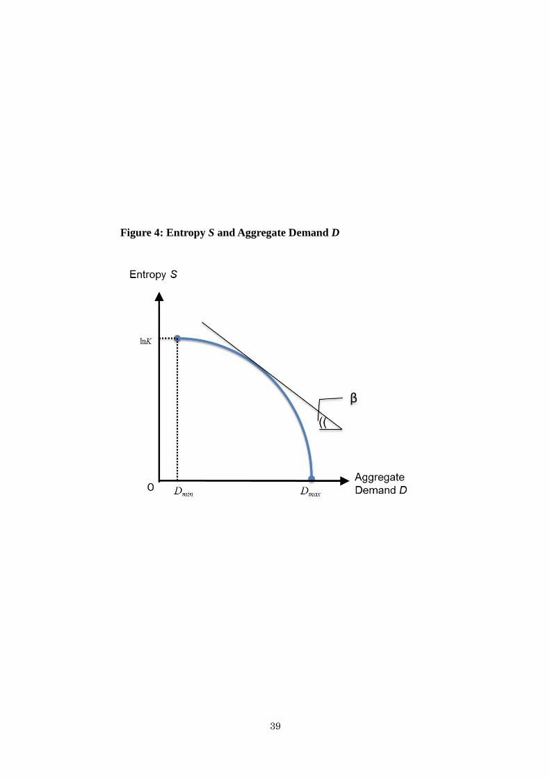
39

Figure 4: Entropy S and Aggregate Demand D

40

Figure 5: Distribution of Labor across Sectors with Different Productivity

― : β＝ - 1/5000 --- : β＝ - 1/7500

41

Figure 6: Distribution of Labor Productivity in Japan (2007)

(a)

Mean= 1.29×104, Standard Deviation=2.37×104

(b)

Mean= 1.30×104, Standard Deviation=2.21×104

42

Figure 6: Distribution of Labor Productivity in Japan (2007)

(c)

Mean= 1.28×104, Standard Deviation=2.48×104

43

Figure 7: Model of Stochastic Macro-equilibrium (a) Dynamics of Creation and destruction of Potential Jobs

Note: Both productivity and the number of potential job sites are in the natural logarithm. The

straight line as drawn in the figure means that the distribution of productivity is

power-law.

(b) Stochastic Macro-equilibrium

The number of potential job sites (in log)

Productivity (in log)

The number of potential job sites (in log)

Productivity (in log)

The Number of Employed Workers

The Level of Productivity

Aggregate Demand D or β

Pool of UnemploymentReservation

wages μ

The Number of Employed Workers

The Level of Productivity

Aggregate Demand D or β

Pool of UnemploymentReservation

wages μ

44

Figure 8: Distribution of labor Productivity

Note: (A) High Aggregate Demand, (B) Low Aggregate Demnd

See the main text for details.

The number of employed workers

(A)

(B)

45

Figure 9: Percentage of Potential Job Sites Occupied by Employed Workers Note: (A) High Aggregate Demand, (B) Low Aggregate Demnd

See the main text for details.

Ratio of employed workers to potential job sites

(A)

(B)

46

Figure 10: Indices of exports and the Industrial Production, normalized to 100 for 2005

Source: Cabinet Office, Ministry of Economy, Trade and Industry

60

70

80

90

100

110

120

130

2006 2007 2008 2009

(2005=100)

Exports

Industrial Production

47

Figure 11: (a)

(b)

48

Figure 11: (c)

49

References Aoki, M. and H. Yoshikawa, (2007), Reconstructing Macroeconomics: A Perspective

from Statistical Physics and Combinatorial Stochastic Processes, Cambridge, U.S.A., Cambridge University Press.

Aoyama, H., H. Yoshikawa, H. Iyetomi, and Y. Fujiwara, (2010), “ Productivity Dispersion: Facts, Theory, and Implication”, Journal of Economic Interaction and Coordination, Vol. 5, pp. 27-54.

Arrow, K. and G. Debreu (1954), “Existence of an Equilibrium for a Competitive Economy,” Econometrica, Vol.22, No.3, pp.265-290.

Asplund M. and V. Nocke (2006), “Firm Turnover in Imperfectly Competitive Markets,” Review of Economic Studies, Vol.73, pp295-327.

Barlevy (2002), Burdett K. and D. T. Mortensen (1998), “Wage Differentials, Employer Size, and

Unemployment,” International Economic Review, Vol.39, No.2, pp257-273. Champernowne, D. (1953), “A model of Income Distribution,” Economic Journal,

Vol.83, pp.318-351. Davis, S. J., J. C. Haltiwanger and S. Schuh (1996) Job Creation and Destruction,

Cambridge, Mass.: MIT Press. DelliGatti, D., E. Gaffero, M.Gallegatti, G. Giulioni and A. Palestini (2008), Emergent

Macroeconomics: An Agent-Based Approach to Business Fluctuations, Milano: Springer.

Diamond, P. (1982), “Aggregate Demand Management in Search Equilibrium,” Journal of Political Economy, Vol.90, pp.881-894.

——— (2011), “Unemployment, Vacancies, Wages,” American Economic Review Vol.75, pp.63?-655.

Fay, J.A. and J.L. Medoff (1985), “Labor and Output over the Busines Cycles: Some Direct Evidence,” American Economic Review Vol.101, No.4, pp.1045-1072.

Feynman, R. P., (1964), “The Principle of Least Action,” Chapter 19 of his Lectures on Physics Vol.II, Reading MA: Addison Wesley.

Foley, D. (1994), “A Statistical Equilibrium Theory of Markets,” Journal of Economic Theory, Vol.62, pp.321-345.

Garibaldi U. and E. Scalas (2010), Finitary Probabilitic Methods in Econophysics, Cambridge: Cambridge University Press.

Hagedorn M. and I. Manovskii (2008) “The Cyclical Behavior of Equilibrium Unemployment and Vacancies Revisited,” American Economic Review, Vol. 98,

50

No.4, pp. 1692-1706. Hicks, J. R. (1936), “Mr. Keynes’s Theory of Employment.” Economic Journal 46

(182): pp.238–253. Houthakker H., (1955/56), “The Pareto Distribution and the Cobb-Douglas Production

Function in Activity Analysis”, Review of Economic Studies, Vol.23, No.1, pp.27-31.

Ijiri Y. and H.A. Simon, (1975) “Some distributions associated with Bose-Einstein statistics”, Proceedings of the National Academy of Sciences of the United States of America, 72(5): pp.1654-1657.

——— and ———, (1979), Skew Distribution and the Size of Busines Firms, Amsterdam: North-Holland.

Ikeda Y. and W. Souma, (2009) “International Comparison of Labor Productivity Distribution for Manufacturing and Non-manufacturing Firms”, Progress of Theoretical Physics, Supplement 179, pp.93-102.

Iyetomi, H. (2012), “Labor Productivity Distribution with Negative Temperature”, Progress of Theoretical Physics, Supplement, No.194, pp.135-143.

———, Y. Nakayama, H. Yoshikawa, H. Aoyama, Y. Fujiwara, Y. Ikeda and W. Souma (2011), “What Causes Business Cycles? Analysis of the Japanese Iindustrial Production Data,” Journal of The Japanese and International Economies, Vol.25, pp.246-272.

Keynes, J. M. (1936), General Theory of Employment, Interest, and Money, London: Macmillan.

Kirman, A.P. (1992) “Whom or What Does the Representative Individual Represent?,” Journal of Economic Perspectives, Spring Vol.6, No.2, pp.117-136.

Kittel, C and H. Kroemer, (1980), Thermal Physics, Second ed., San Francisco: W H Freeman.

Kydland, F. and E. Prescott, (1982), “Time to Build and Aggregate Fluctuation,” Econometrica, November.

Marsil M. and Y. C. Zhang, (1998), “Interacting Individuals Leading to Zipf’s Law,” Physical Review Letters, 80, No.12, pp.2741-2744.

Mankiw N. G. (1989), “Real Business Cycles: A New Keynesian Perspective,” Journal of Perspectives, Vol.4, No.3, 79-90.

——— and D. Romer (1991), New Keynesian Economics, Vol.1 and 2, Cambridge: The MIT Press.

Modigliani, F., (1944), “Liquidity Preference and the Theory of Interest and Money,” Econometrica Vol.12, No.1, pp.45-88.

51

Mortensen, D.T., (2011), “Markets with Search Friction and the DMP Model,” The American Economic Review Vol.101, No.4, pp.1073-1091.

Negishi, T. (1960-61), “Monopolistic Competition and General Equilibrium,” Review of Economic Studies, Vol.28, pp.196-201.

——— (1979), Microeconomic Foundation of Keynesian Macroeconomics, Amsterdam : North-Holland Publishing.

Okun, A (1963), “Potential GNP: Its Measurement and Significance,” Proceedings of the Business and Economic Statistics Section, American Statistical Association, 98-104, reprinted in Okun’s The Political Economy of Prosperity, Washington D.C.: The Brookings Institution, 1970.

——— (1973) “Upward Mobility in a High-pressure Economy,” Brooking Papers on Economic Activity, Vol. 1, pp.207-261.

Pissarides, C.A., (2000), Equilibrium Unemployment Theory, second edition, Cambridge: The MIT Press.

――― (2011) “Equilibrium in the Labor Market with Search Frictions,” The American Economic Review Vol.101, No.4, pp.1092-1105.

Postel-Vinay, Fabien and Jean-Marc Robin, (2002), “Equilibrium Wage Dispersion with Worker and Employer Heterogeneity,” Econometrica Vol.70, No.6, pp.2295-2350.

Ramsey, N. F., (1956), “Thermodynamics and Statistical Mechanics at Negative Absolute Temperatures,” Physical Review, 103, No.1, pp.20-28.

Rogerson, Richard, Robert Shimer, and Randall Wright, (2005), “Search Theoretic Models of the Labor Market: A Survey,” Journal of Economic Literature, Vol.XLIII, December, pp.959-988.

Sato, Kazuo, (1974), Production Functions and Aggregation, Amsterdam: North-Holland.

Shimer R. (2005) “The Cyclical Behavior of Equilibrium Unemployment and Vacancies,” American Economic Review, Vol. 95, No.1, pp. 25-59.

Solow R. M. (1986) “Unemployment: Getting the Questions Right,” Economica, Vol. 53, Supplement, pp. S23-34.

Summers, L.H. (1986) “Some Skeptical Observation on Real Business Cycle Theory,” Federal Reserve Bank of Minneapolis Quarterly Review, Vol. 10, 23-27.

Syverson, C. (2011) "What determines productivity?" Journal of Economic Litereture, Vol.49, No.2, pp.326-365

Tobin, J. (1972), “Inflation and Unemployment,” American Economic Review. Vol. 62, pp. 1-18.

――― (1993) “Price Flexibility and Output Stability: An Old Keynesian View,”

52

Journal of Economic Perspectives, Vol.7, pp.45-65. Yoshikawa, H., (2003), “The Role of Demand in Macroeconomics,” Japanese

Economic Review, 54, (1), pp.1-27.