EQUILIBRIUM AND EXTINCTION IN STOCHASTIC POPULATION …

Bulletin of Mathematical Biology Vol. 49, No. 6, pp. 67Hi96, 1987. Printed in Great Britain.

0092-8240/87S3.00 + 0.00 Pcrgamon Journals Ltd.

cl:: 1987 Society for Mathematical Biology

EQUILIBRIUM AND EXTINCTION IN STOCHASTIC POPULATION DYNAMICS

• H. RoozEN Centre for Mathematics and Computer Science, P.O. Box 4079, 1009 AB Amsterdam, The Netherlands

Stochastic models of interacting biological populations, with birth and death rates depending on the population size are studied in the quasi-stationary state. Confidence regions in the state space are constructed by a new method for the numerical solution of the ray equations. The concept of extinction time, which is closely related to the concept of stability for stochastic systems, is discussed. Results of numerical calculations for two-dimensional stochastic population models are presented.

1. Introduction. This paper describes properties of stochastic population systems defined by birth and death rates depending on the population size. The state variables are the non-negative population numbers, so that the state space is formed by the positive orthant and its boundary. The deterministic dynamical system associated with the stochastic system is assumed to have a stable equilibrium point lying in the interior of the state space. For large population sizes the statistically quasi-stationary state of the stochastic system is described by a probability density function (p.d.f.) defined on the state space, with a maximum at the equilibrium point. Close to the equilibrium point this p.d.f. is approximately multivariate Gaussian. At a larger distance, deviations from the Gaussian shape become pronounced. Part of this paper deals with the construction of the contours of the associated confidence regions in state space. A method has been developed for the numerical solution of the ray equations, needed in the computation of the contours. The method does not have the disadvantages of the numerical methods that are normally used to solve the ray equations, such as the initial value approach or shooting methods.

An important concept in stochastic population dynamics is the concept of stability. Once a stochastic system of populations is caught within the attraction domain of a stable equilibrium point of the corresponding deterministic system, it will remain there for a long time, attracted by the equilibrium point. Stochastic fluctuations give rise to deviations from the equilibrium point. Large departures may occur, which can lead to escape from the domain of attraction of the equilibrium. With probability one this will happen within a finite time. On hitting the boundary of the state space by stochastic fluctuations, the domain of attraction is left: one population becomes extinct. The birth and death rates for that population are zero, the boundary is absorbing. The ecological stability of a system is expressed in terms

671

672 H. ROOZEN

of the mean extinction time, for which expressions are given. A related problem that will be touched upon is which of the populations of a stochastic system is expected to become extinct first.

In the second part of this paper the foregoing theory is applied to a stochastic system consisting of two interacting populations. The associated deterministic system is a generalized Lotka-Volterra system with two components. A systematic treatment of this system is given. The stability condition for the interior equilibrium point is derived. Close to the equilibrium the quasistationary state of the stochastic system is approximately described by a twodimensional Gaussian p.d.f. The parameters of this Gaussian p.d.f. are expressed in the parameters of the stochastic model. As a consequence, some conclusions about the behaviour of the stochastic model can be drawn. For a number of particular cases, contours of confidence regions in the state space are depicted. There is a good agreement with the results of numerical simulations of the original stochastic birth and death processes. Finally, the concept of extinction is treated. Results obtained by the ray method and by the approximate method in which the p.d.f. is assumed to be Gaussian, are compared with the data, obtained by the numerical simulations.

2. Derivation of the Fokker-Planck Equation. In this section the FokkerPlanck or forward Kolmogorov equation is derived. This is a transport equation for the joint probability density function for the number of individuals in each of the populations of a population system at time t. First a system with a single population is considered. Then the straightforward generalization to n populations is made.

One population. Let the number of individuals in a single population at some time t be given by the non-negative integer N. Assume that the population has an infinitesimal birth rate B(N) and an infinitesimal death rate D(N). This means that the probability of a single birth or death in the small time interval (t, t + ..1.t) is given by B(N)At and D(N)t:.t. The probability of multiple births and deaths in the time interval is proportional to (f:.t )2 and may be neglected for small At. The probability P(N, t) of having N individuals at time t, satisfies the equation:

P(N, t+..1.t)=P(N-1, t)B(N-1) At+ P(N + 1, t)D(N + 1) t:.t

+P(N,t)[l-{B(N)+D(N)}f:.t]. (1)

Thus the number of individuals at some time is obtained by either one of three mutually exclusive events in the foregoing small time interval oflength t:.t, i.e. a birth, a death, neither birth nor death. In the limit M~o the master equation is obtained:

EQUILIBRIUM AND EXTINCTION IN STOCHASTIC POPULATION DYNAMICS 673

a/5~, t) = P(N-1, t)B(N-1)+ P(N + 1, t)D(N + 1)-P(N, t){ B(N) + D(N)}.

(2)

In this way a discrete state space Markov process has been defined. An approximating process in a continuous state space is constructed in the following way. A new population variable x = N/ K is introduced by scaling N with Kand the corresponding p.d.f. P(x, t) is defined by

P(N, t)=Pr{N- ~ ~N(t)::;;N + n=Pr{x- 2~::;; x(t):S;x + 2~} 1

= P(x, t) [(" (3)

The parameter K is typical for the population size. A natural choice is the size of the equilibrium of the deterministic system, which by assumption is large. Then x may approximately be treated as a continuous variable and functions of x as continuous functions. With

B(N) = B(xK) = B(x),

D(N) = D(xK) = D(x ),

we obtain from the master equation:

(4)

ap~~' t) = p( x - ~, t)B(x- ~)+P(x + ~· t)D(x +~)-P(x, t){B(x)

+ D(x)}. (5)

The birth and death rates B and D are assumed to be expressible in van Kampen's (1981) canonical form, that is, in a power series in K- 1 of the following kind:

B(x)=f(K)[ 0B(~)+ 1B(~)K- 1 + 2B(~)K-2+ .. J D(x)=f(K) [ oD(~)+ 1D(~)K- 1 + 2D(~)K- 2 + · · ·l (6)

It is assumed that Band Dare smooth functions. By a Taylor series expansion (Kramers-Moyal expansion) of the functions on the right side of equation (5) up to second order in K- 1 , the following Fokker-Planck equation is obtained:

_1_ aP(x, t) = _ _!_ ~ [{(o B(x)- o D(x)) + _!_ (1B(x)-1 D(x)) f(K) at K ax K

674 H. ROOZEN

+ ~2 ::2 [ { ( 0 B(x) + 0 D(x))

+2- (1B(x)+ 1D(x)) K

+ ~2 (2B(x)+ 2D(x))+ · · ·}P(x, t)l In the simple case that

f(K)=K,

iB(x)=. iD(x)=.O, for i>O,

so that B and D are given by

B(x)=K. 0s(~}

D(x)= K. 0D(~} the Fokker-Planck equation takes the form

oP~~, t) = - :x [{ 0 B(x)- 0 D(x)}P(x, t)]

1 a2

+ 2K ox2 [{OB(x)+ OD(x)}P(x, t)].

(7)

(8)

(9)

(10)

The first term on the right side expresses the drift of the system, the second one the diffusion. For large values of K the diffusion is small compared to the drift.

The approximating continuous process and the original discrete process have the same first and second jump moments. However, as a consequence of truncating the Taylor expansion after two terms, higher moments do not agree. The higher moments of the continuous process are all zero, while for the discrete process the odd moments are equal to the first moment and the even moments are equal to the second moment.

An approximation to birth-death processes incorporating higher jump moments can be found in Knessl et al. (1984, 1985). The methods described in this paper are also applicable to that approximation, as it gives rise to a Hamilton-Jacobi system similar to (28).


n populations. For every population i from a system of n populations, the birth rate is B;(Np N 2, ... , Nn) and the death rate is DJNP N2 , .•• , Nn). Let the B;(Xp x 2 , ..• , xn) and the D;(Xp x2 , •.. , xn) be defined by

B;(Np N2, ... 'Nn)=B;(X1K1, X2K2, ... 'xnKn)=B;(xl, Xz, ... , x.),

D;(Np N 2 , ••• , Nn)=D;(x 1Kp x 2K2, ••• , x,.Kn)=D;(x 1, X2, ... , x,,). (11)

New variables X; = N J K; were introduced by scaling the old ones by the sizes of the equilibrium populations. On assuming the canonical forms

o (Ni Nz Nn) B;(xp Xz, ... 'xn)=K;. B; Kl' Kz' ... 'Kn '

D;(x 1 , x2 , ••. , xn)=K;. 0 D;(!!.l, N2 , .•• , N"), (12) K1 K2 K.

the following Fokker-Planck equation is obtained:

aP(x 1 ,x2 , .•. ,Xn,t) at

=L -[{0B;(X1,X2,···,xn) n {-a i=l axi

- 0 D;(x1' Xz, ... 'xn)}P(xl' Xz, ... 'xn, t)]

1 a1

+--z({oB;(X1,X2, ... ,xn) 2K; ax;

+ 0 D;(x1, x 2 , ..• , x.)}P(x 1 , x2 , .•• , xn, t)J }·

The population sizes K; are assumed to be large and of equal order:

K;= o(l). (s small)

so that

Substitution in the Fokker-Planck equation gives:

oP(x t) n [ a } c: 02 { ( )\] ·' = L - - {b;(x)P(x, t) + -2 ;12 a;(x)P x, t J ,

at i= 1 ax; vX;

in which

(13)

(14)

(15)

(16)

676 H. ROOZEN

b;(x)= o B;(x)- 0 D;(x),

a;(x) = K;( 0 B;(x) + 0 D;(x)).

(17a)

(17b)

This form of the Fokker-Planck equation, valid for a system of n populations having large equilibrium values of equal order, is the starting point of our analysis.

For very large populations the diffusion term may be neglected. The system is then described by the Liouville equation:

oP(x, t) =I [-J_ {b;(x)P(x, t)}J. at i=l axi

(18)

It can be shown (Gardiner, 1983) that this equation with initial condition

(19)

describes a deterministic motion which can also be found by solving the system of differential equations:

dx;(t) b ( ) . 1 2 ~= ;X,l=, , ... ,n (20)

with initial conditions

(21)

This system of differential equations defines the deterministic system associated with the Fokker-Planck equation. The equilibrium points of the deterministic system are found by putting

b;(x)=O, i= 1, 2, ... , n (22)

that is, by equating birth and death rates.

Boundary classification. For one-dimensional stochastic systems a complete classification of boundaries exists (Gardiner, 1983; Feller, 1952; Roughgarden, 1979). In order for the one-dimensional population system to have an exit boundary at x=O, the following conditions must be satisfied:

J(O, t)<O,

b(O) = 0, a(O) = 0,

in which J is the probability current defined by

(23a)

(23b)


called rays. All rays emanate from the equilibrium point. Rays may be interpreted as paths of maximum likelihood joining (points in the neighbourhood of) the equilibrium point with points in x-space. See Ludwig (1975) and the references given there.

Local analysis near the equilibrium. In the neighbourhood of the equilibrium point of the ray equations, Q is approximated by a quadratic form:

(34)

in which Pii is a symmetric matrix:

(35)

Differentiation of expression (34) gives an approximation for the r;:

oQ . P; =-;---~I P;/xj-1), z = 1, 2, ... , n.

vX; j (36)

The deterministic vector field b; near the equilibrium point is approximated by

(37)

Substitution of the approximations (36) and (37) in the eikonal equation gives:

(38)

Making use of the symmetry of Pii' this can be rewritten in the matrix form:

PAP+PB+B'P=O, (39)

in which B= (obj8xi), t denotes the transpose and A is a diagonal matrix containing the values of a; at the equilibrium point. Left and right multiplication with S= p- 1 gives:

A+BS+SB'=O. (40)

If the matrices Sand A are written column wise as vectors, a linear system with n 2 equations is obtained, which can be solved for S. The matrix P is obtained by inversion of S. All eigenvalues of B are negative, because of the assumed stability of the equilibrium point of the deterministic system. C onseq uen tly, the last two operations can be carried out. The elements of the matrix P can be

680 H. ROOZEN

substituted in expression (34), resulting in an approximation of Q in the neighbourhood of the equilibrium point.

Confidence regions. From the Ansatz (27) it is clear that contours of constant Q (hypersurfaces) in the state space, are contours of constant probability. Let Qz be the value of Q corresponding to the contour, for which the probability of being in the region R enclosed by this contour, is equal to z:

LP.(x') dx' =z, O:::;;z:::;; 1. (41)

In order to construct the contour enclosing the confidence region of probability z, the corresponding value Qz of Q has to be determined. The following heuristic method is used. According to the local analysis, in a first approximation Ps has an n-variate normal distribution around the equilibrium point, given by

( Q(x)) P.(x)=Cexp --8-. (42)

Then by a standard result in probability theory (Hogg and Craig, 1970), 2Q(x)/e has a chi-square distribution with n degrees of freedom. The value 2Qz/e which will not be exceeded by 2Q(x)/e with probability z, can be found in a table of the chi-square distribution with n degrees of freedom. In the case n = 2, used in the examples in Section 5, the chi-square distribution has a simple form from which it can be derived that

Qz= -eln(l-z). (43)

Numerical solution of the ray equations. The local analysis near the equilibrium point may not be a sufficiently accurate approximation away from this point. Then the ray equations have to be solved numerically.

(i) The initial value approach For the system (32) a starting point x(O) at s = 0 is chosen close to the equilibrium point. The formulas (34) and (36) give the initial values for Q and Pi (i= 1, 2, ... , n). The ray equations are solved numerically by using a routine for solving a system of ordinary differential equations written in first-order form with conditions in the form of initial values. For this purpose the NAGlibrary contains Runge-Kutta Merson routines or variable order, variable step Adam routines. On applying such a routine, the solution Q(s), xi(s), Ph) (i = 1, 2, ... n) is obtained along the ray defined by the initial point x(O). Once


the initial point has been chosen, there is no control over the way the ray develops through space. Generally there is a very strong dependence on the initial point. Especially when the eigenvalues of the deterministic system in the equilibrium point do not have ratios close to one, it is impracticable to choose the initial points in such a way that a bundle of rays is obtained, which uniformly covers the state space around the equilibrium point. Thus, the method is not well suited for the construction of the contours of the confidence regions.

Even shooting methods, in which the initial point is manipulated systematically as to obtain the desired rays, did not solve the difficulty (Ludwig, 1975).

(ii) The boundary value approach Instead of specifying the 2n + 1 conditions at a starting point close to the equilibrium, n + 1 conditions are imposed at the starting point coinciding with the equilibrium and n conditions are imposed at an endpoint which can be chosen freely:

S---+-oo: Q=O,X;=l, i=l,2, ... ,n

s=O: X;=e;, i= 1, 2, ... , n

(44a)

(44b)

where thee; are the coordinates of the endpoint. At s---+ - oo the condition for x has been retained and that for p has been dropped. This choice is understood as follows. Trajectories of (32ab) exist, that for decreasing s leave a neighbourhood of the equilibrium point and in the limits---+ - oo approach the subspace with negative eigenvalues. Condition (44a) forbids such solutions.

The limit s---+ - oo (in numerical computations replaced by s= -s*, s* a sufficiently large number) will cause the characteristic to start at (close to) x = 1, p = 0. The characteristic lies in the unstable manifold through x = 1, p =0. It can be shown (Roozen, 1986) that the plane tangent to this manifold at this point satisfies (39), so that the boundary value solution corresponds to an initial value solution.

The two point boundary value problem thus described is solved by using an appropriate routine, for example the NAG~routine D02RAF. This routine uses a deferred correction technique and Newton iteration. On a grid of s-values, a first approximation to the solution has to be given, from which the routine iteratively tries to find the solution. Experience has shown that the method works well provided that a good first approximation is given and a sufficient number of grid points are used.

Endpoints may exist, for example in the neighbourhood of a caustic, which can be connected with the equilibrium by more than one characteristic. In that case, the characteristic that is constructed by the boundary value approach depends on the first approximation to the solution.

682 H. ROOZEN

Because the endpoints can be chosen at will, contours of confidence regions can be constructed by this method quite efficiently. The contours and rays of the stochastic two population models shown in Section 5 of this paper, have been obtained by this method. Details of the numerical construction of rays and contours can be found in Roozen (1986).

4. Extinction. In this section, exit from a region R with boundary Sis treated. Questions of interest are the following. What is the expected first exit time and which population is expected to exit first? In the birth-death models treated in this paper, exit at the boundary X;=O means extinction of population i.

The expected time of first exit T(x ), starting in a point x in a region R with boundary S, satisfies the Dynkin equation, which can be derived from the backward Kolmogorov equation (Gardiner, 1983; Schuss, 1980) and is given by:

~ {b.( ) oT(x) !'._ .( ) 8 2 T(x)} = - l L., ! x a + a, x a 2 • i= 1 X; 2 X;

It has to be solved with the boundary condition

The problem is rewritten as

T(x)=O for xES.

LeT= -1 in R

T=O on S.

(45)

(46)

(47)

The operator Le is the formal adjoint of the operator on the right side of equation (16) working on the p.d.f.

The probability P(x, x') of exit at x' ES, starting from x ER is related to the solution u(x) of the boundary value problem:

u =f(x) on S (48)

by the relation

u(x)= JJ(x')P(x, x') dSx'· (49)

After choosing the functionf, we can solve the problem (48) and obtain the corresponding function u(x). If for examplef(x')=l>(x'-a), then by solving (48), u(x)=P(x, a) is obtained.


In the asymptotic analysis for smalls, see Ludwig (1975), Matkowsky and Schuss (1977), it follows for the expected exit time that

(50)

in which x* ES is the boundary point at which Q takes its minimal value at the boundary. The most likely point of exit is the boundary point x*. The asymptotic results have been derived for the case that at the boundary S the trajectories of the deterministic system enter the region R.

In the study of extinction the boundaries xi = 0 (i = 1, 2, ... , n) are of interest. If xi=O is the boundary which contains x*, then i is the population which most likely will get extinct first. However, in the application to the birth and death models, some complications arise. At xi = 0 (i = 1, 2, ... , n) the trajectories of the deterministic system remain in the boundary xi=O. The functions ai(x) and bi(x) tend to zero at the boundary xi=O, which requires a new type of local asymptotic analysis. As a consequence of the fact that ai(x) and bi(x) vanish near the boundaries, the rays there deflect and large gradients in the ray variables are found.

The problems are avoided by studying the mean time needed for a system of populations to reach one of the small positive levels xi =Ii (i = 1, 2, ... , n ), assuming the WKB-Ansatz to be valid for xi ~Ii (i = 1, 2, ... , n ). The computation of x* and Q(x*) can be carried out efficiently by using a variant of the boundary value approach. With respect to the boundary xi =Ii the boundary conditions are:

s-+-oo: Q=O,xi=l, j=l,2, ... ,n

s=O: xi=li,pi=O, j=l,2, ... ,nandj#i. (51)

The variant of the boundary value approach with conditions (51) has to be solved for each of the boundaries xi= li (i = 1, 2, ... , n). The boundary at which the smallest value for Q is found is the expected exit boundary and the point on this boundary where this value is taken is the expected exit point. For the details of the numerical solution, see Roozen (1986).

5. A stochastic two population model. In this section the theory is applied to a stochastic two population model. The model under consideration is described by birth and death rates of the form:

B1(N1, Nz)=N1P'1o+l11N1 +l12N2)

B2(N1, N1)=N2(A2o+l21N1 +l22N2)

Di (N1, Nz)= Ni (µ10 + µuN1 + µ12N2)

D1(N1, N1)=N2(µ20+µ21N1 +µ22Nz), (52)

684 H. ROOZEN

in which the)... andµ .. are constants, such that the birth and death rates are I) I]

positive for all admitted values of N1 and N2 .

The deterministic system. In the original variables N 1 and N 2 , the deterministic system is given by the generalized Lotka-Volterra system:

d:r1 =N1(h1o+h11N1 +b12N2)

dN2 dt=N2(h20+h21N1 +h22Nz), (53)

in which bu= 1, A;j-µ;/or i = 1, 2 andj=O, 1, 2. The equilibrium populations K 1 and K 2 are given by

K _ b22b10-b12b20 K _ b11b20-b21b10 1 -b b b b ' 2 -b b b b 21 12- 11 22 21 12- 11 22

(54)

Introduction of new variables

N. x.=~ i=l 2 ' K.' ,

' (55)

gives:

(56)

in which:

(57)

Assuming that both populations have a self-limiting growth (i.e. that b11 and b22 are negative) the factors k1 and k2 are positive. They can be interpreted as the reciprocals of time scales for the respective populations. The type of interaction between the populations is determined by the parameters ix and fi as shown in Fig. 1.

For the subsequent analysis it is important to know the condition under which the equilibrium of the deterministic system at (1, 1) is stable. Linearization of the system b 1(x1' x 2), b 2(x 1, x 2 ) which is given by equations (56), in the neighbourhood of the equilibrium point gives:


predatorprey

mutual ism

0

competition

predatorprey

Figure 1. The type of interaction between the two populations depending on the parameters oc and {3.

dx B-- = x dt '

in which x = (x 1 -1, x 2 -1)1 and the matrix Bis given by

-ak1] -k .

2

The eigenvalues of Bare:

(58)

(59)

(60)

The condition for stability is that the real parts of the eigenvalues are negative, resulting in

a/3< 1. (61)

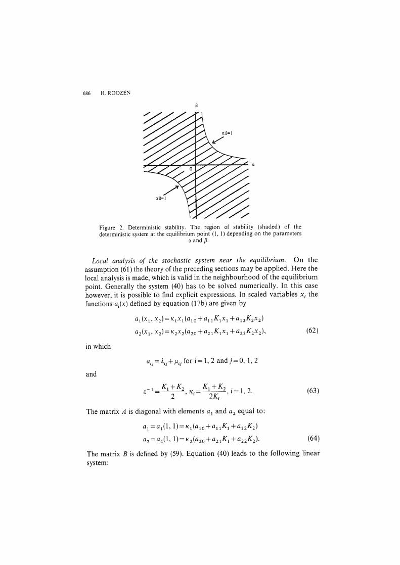
Figure 2 shows the region of stability in the oc,{3-parameter plane. From Figs 1 and 2 it can immediately be concluded that the equilibrium (1, 1) is stable for all predator-prey models, while for mutualism and competition models this equilibrium is stable for parameter values of oc and /3 in only a small region of the oc,{3-parameter plane.

The same kind of stability analysis as given above can be carried out for the equilibrium points at (0, 0), (1 +a, 0) and (0, 1 + /3), which are of interest only if both coordinates are non-negative. It can be shown that also for these equilibrium points the type of stability depends on oc and /3 only.

686 H. ROOZEN

Figure 2. Deterministic stability. The region of stability (shaded) of the deterministic system at the equilibrium point (1, 1) depending on the parameters

a and fl.

Local analysis of the stochastic system near the equilibrium. On the

assumption (61) the theory of the preceding sections may be applied. Here the

local analysis is made, which is valid in the neighbourhood of the equilibrium

point. Generally the system (40) has to be solved numerically. In this case

however, it is possible to find explicit expressions. In scaled variables X; the

functions a;(x) defined by equation (l 7b) are given by

in which

and

al(.xl, X2)=K1X1(a1o+a11K1X1 +a12K2X2)

az(X1, X2)= KzX2(a20 +a21K1X1 +a22K2Xz),

- i - K1 + K1 . - K1 + Kz . -1 2 i; - 2 ' K; - 2K. ' l - ' •

!

The matrix A is diagonal with elements a 1 and a2 equal to:

a1 =a 1(1, l)=K1(a 10 +a 11 K 1 +a 12 K2 )

a2 =a2 (1, l)=K2(a20 +a21 K1 +a22 K2 ).

(62)

(63)

(64)

The matrix Bis defined by (59). Equation (40) leads to the following linear

system:


-2kl -ak1 -ak1 0 S11 -a1

-fik2 -kl -k2 0 -ak 1 8 21 0 = (65)

-fik2 0 -k1 -kz -rxk1 S12 0

0 -fik2 -fik2 -2k2 822 -a2

The solution of this system is given by

The matrix P in expression (34) is found by inversion of the matrix S:

By using (42) the bivariate normal p.d.f. is determined. The corresponding confidence contours in the state space are ellipses. In some special cases the expression for P can be simplified. For example, the competition model, treated by May [1974, p. 123-129], is a particular case of our more general model. The p.d.f. derived by May is easily found from the formulas given above.

The expressions show the complex dependence of the ellipses on the parameters k1 , k2 , a, fi of the deterministic system and the noise components a 1

and a2 at the equilibrium point. It may be noted that multiplication of k 1 , k2 , a 1 , a2 with the same constant leaves the resulting p.d.f. invariant. The effect of an increase (decrease) of velocity by which the system returns to the deterministic equilibrium cancels the effect of an increase (decrease) of the stochastic fluctuations.

The covariance matrix corresponding to a bivariate normal distribution is given by Batschelet (1981):

(68)

in which ai and a~ are the variances and p is the correlation coefficient. On equating this matrix to the actual covariance matrix E:S, the following expressions for the variances and the correlation coefficient are obtained:

688 H. ROOZEN

2 a1k2 [k 2 +k 1(1-a{J)]+a 2a2kt CT 1 = e k ) ( R) ' 2k 1k2 (k 1 + 2 1-ap

(69)

2 a2k1[k 1 +k2 (1-a{J)]+a 1{J2ki a2 = e 2k1k2 (k 1 +k2 ) (1-a{J) '

(70)

= -(a 1/Jki+a 2akt) . (7l) P J{a 1 k2 [k2 + k 1 (1-a/3)] +a2a2k;} {a2k1[k1 + k2 (1-a{J)] + a1{J 2 ki}

Note the dependence of the first two expressions on e, the reciprocal of the mean of the equilibrium populations. The parameters k1 , k2 , a 1 , a2 , e are all positive. The condition for a stable equilibrium is that 1-a/J is positive. Then, it is easily seen that the sign of the correlation coefficient p equals the sign of the numerator on the right side of equation (71 ), from which it follows that for competition (a> 0, f3 > 0) the correlation coefficient is negative and for mutualism (a<O, /3<0) the correlation coefficient is positive. For predatorprey systems both positive and negative values are possible.

For the cases that the local analysis is also valid far from the equilibrium, an expression for the expected exit time can be derived. Let Ci be the minimal value of Q in equation (34) for which the ellipse touches the axis xi = 0 and define T; by

(72)

It can easily be shown that

(73)

T - {1 (k 1 +k2 )k 1k2(1-af3) }- l/la2 2 -exp - 2 2 - e 2.

e a1/3 k2 + a2k2 [k 1 + k2 (1-a{J)] (74)

The last equalities in (73) and (74) follow from (69) and (70). For the expected extinction time T it follows 'that

(75)

The ecological stability index~. defined in Nisbet and Gurney (1982, p. 10) by

~=ln T (76)

then satisfies:

- ·(1 1) ~ "' ~ =mm 2o'f' 2a~ · (77)


Recalling that scaled population variables are used, this result can be seen as a two-dimensional generalization of the one-dimensional result in Nisbet and Gurney (1982, p. 202).

Given the values of a 1, a2 , k1 , k2 it may be wondered which combination of a and {J leads to the largest ecological stability. Figure 3 shows the curves of equal ~ in the a, {J-parameter plane. Typically, the largest ecological stability is found in predator-prey systems. As an illustration of the different meaning of stability in deterministic and stochastic systems, Fig. 3 should be compared with Fig. 2.

8 8

Fig. 3. Stochastic stability. Curves of equal~. derived from the local analysis, in th_e oc,f:l-parameter plane. The arrows indicate increasing values of~- The difference in~ -values between successive curves in each of the figures is constant. In the atypical case a1/k 1 =a2/k2 the maximum of~ is adopted on f:I= -a 1oc/a 2, which is a line through the origin with a negative slope. Fig. 3a shows a case a1/k 1 r::::-a 2/k 2 and Fig. 3b shows a case a1/k 1 '::j:,a 2/k 2 • The actual valuesofaP a 2 , kp k2 are 1.0, 1.3, 1.1,

0.8 for case a and 1.0, 8.0, 1.1, 0.7 for case b.

Apart from the time to extinction it may be convenient to have an expression for the expected time for a system of populations to reach one of the levels xi = l; (expressed in units of the equilibrium populations) with l; not necessarily equal to zero. It is found that with

(78)

the expected time T satisfies:

(79)

The points of contact of the ellipses with the axes x 1 =11 and x 2 =12 are given by

P12 I ) X 1 =11, X 2 =1 +p (1- 1

22

(80)

690 H. ROOZEN

TABLE I (A) The Birth and Death Rates for Three, Two-population Models.

(B) Parameters of the Corresponding Deterministic System.

2 3 Predator-prey Mutualism Competition

A (),ij) 1. . 004 0 . .6 .004 .0056 l. .004 0. .6 . 0056 0 . .8 .0016 .0016 . 8 0 . .0016

(µ;j) .280 .012 .0064 .480 .012 0. .64 .008 .0032 .480 0 . .008 .480 0 . .0096 .56 .0008 .0056

B IX .8 -.7 .8

f3 -.7 -.2 .2 k, .4 .4 .2 k2 .4 .4 .2 K, 50 50 50 Ki 50 50 50

(A) The coefficients appear in the same order as in (52). (B) The values of the parameters can be calculated from the birth and death rates.

TABLE II Results of Numerical Birth-Death Experiments

Number of Exit at x 1 =0.1 Exit at x 2 = 0.1 -6 experiments log T at x 2 = % of exp at x 1 = % of exp

10 200 2.175 1.14 57 1.21 43 20 200 3.067 1.11 59.5 1.30 40.5 40 150 4.554 l.21 61.3 1.48 38.7 60 50 5.530 1.14 82 l.61 18 80 50 6.879 l.26 94 1.65 6

and

(81)

respectively. In cases that the local analysis is valid only in a small neighbourhood of the

equilibrium, the expressions given here cannot be used. Instead, the full system of ray equations (32) has to be solved numerically.

Construction of contours. For the cases, defined by the birth and death rates in Table I, the ray equations (32) have been solved numerically by the method,


presented in this paper as the boundary value approach. Figure 4 shows the confidence contours and rays for the various cases. The cases I and 3 are similar to the examples 1 and 2 of Ludwig (1975). The difficulties reported by Ludwig in the construction of rays in his second example, the competition model, were also experienced by the author, when the initial value approach was used, in which the initial values were chosen equidistantly on a small circle around the equilibrium point. As a consequence of the fact that the eigenvalues of the

(\JO

"' z..'.. 0

1.00 1.so POPULATION I

Figure 4(a) and (b).

(a)

2 .oo 2.so

(b)

2 .50

692 H. ROOZEN

(c)

0 "?

El o..,_o .~oo---'.=50--1,--'-.o=o---,1.....,.s=o----,o-'=---:-'2 .50

POPULRT ION 1

Figure 4. Rays and confidence contours for (a) the predator-prey model, (b) the mutualism model, (c) the competition model, defined in Table I, as obtained by solving the ray equations by the boundary value approach. From the inside outwards, the three (inner) contours correspond to the 50%, 95% and 99%

confidence regions, respectively.

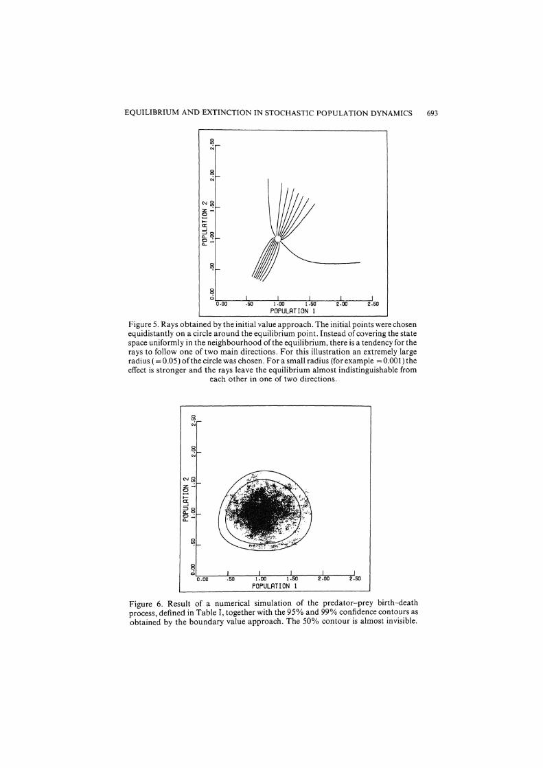
linearized deterministic system at the equilibrium point do not have a ratio close to one [ratio 5.7 in Ludwig (1982)], almost all rays follow very closely and nearly indistinguishable from each other one of two paths, as shown in Fig. 5. The boundary value approach introduced in this paper overcomes these problems, see Fig. 4c. From the figures it is apparent that close to the equilibrium the contours have the elliptic shape, while further away deviations from the elliptic shape tend to come in.

Figure 6 shows the result of a numerical simulation (see the Appendix) of the predator-prey system. Each of about 35,000 dots represents a visit. Because the population sizes can take on only integer values, the dots should lie on a twodimensional grid. However, the dots have been plotted slightly away from their grid positions in a random way, in order to get a good idea of the corresponding p.d.f. The agreement with the constructed contours is quite good.

Exit boundary and exit time. As an illustration of the theory dealing with the expected exit point and the expected exit time, a number of numerical simulations (see the Appendix) have been carried out for the competition model given in Table I, with different values of the noise parameter t:. The results are shown in Table H. The first column shows the value of e - 1 • The second column shows the number of experiments carried out for the corresponding case. Column 3 shows the values found for log T, in which T is


Ii! ·-"'

~ ..... N

NIL ~ z-0 -I-a: ...J

~~ ..... a... -

~ ~-

~ I c I I I I

o.oo .so 1.00 1.so 2.00 2.60

POPULATION 1

Figure 5. Rays obtained by the initial value approach. The initial points were chosen equidistantly on a circle around the equilibrium point. Instead of covering the state space uniformly in the neighbourhood of the equilibrium, there is a tendency for the rays to follow one of two main directions. For this illustration an extremely large radius ( =0.05) of the circle was chosen. Fora small radius (for example =0.00l)the effect is stronger and the rays leave the equilibrium almost indistinguishable from

each other in one of two directions.

~ OL,..-,,o=--~-':::,....-~..,-l::-~-:-'=-~--;;"'=~---,~, o.oo .so 1.00 1.so 2.00 2.so

POPULATION 1

Figure 6. Result of a numerical simulation of the predator-prey birth-death process, defined in Table I, together with the 95% and 99% confidence contours as obtained by the boundary value approach. The 50% contour is almost invisible.

694 H. ROOZEN

log T

8

+

6 ray

+ loc

4

2

0

Figure 7. Relationship between log Tand l/e. The crosses are values obtained by the experiments. The lines correspond to the expressions (82a) and (82b) with

C1oc=C,.y= 1.

the mean time needed for one of the populations of the system to reach 10% of its equilibrium value. The resulting columns 4 and 5 show the mean point of exit at the boundary x 1 =0.1, x 2 =0.1 (in units of the equilibrium values) respectively, with the percentage of exits at that boundary.

The approach based on the local analysis, as described in this paper, indicates that (0.1, 1.31) is the most probable exit point, so that population 1 is expected to exit first. The expected exit time is I'ioc "'e0 ·06062 fe.

Solution of the ray equations, in the way described at the end of section 4, indicates that (0.1, 1.25) is the most probable exit point, so that population 1 is expected to exit first. See Fig. 4c, which indeed suggests that the boundary x 1 = 0.1 is tangent to a contour line in the neighbourhood of (0.1, 1.25 ). The corresponding value of Q is lower than is the case for the contour, to which the boundary x2=0.1 is tangent. The expected exit time is Tray"'e0·07508i'.

As is seen, the mean exit point obtained from the experiments agrees well with the value from the asymptotic theory for small i;. Notice the increasing percentage of exits in the neighbourhood of the predicted place for decreasing values of i; in the experiments. The approach based on the local analysis leads to results which agree reasonably well with the results of the experiments.

We write the relationships between T and i; - 1 as

T, = c e0.06062/e ~c ~c '

T = C eo.07508/e ray ray '

(82a)

(82b)


in which C10c and Cray are constants. In a graph of lnT against e- 1 these relationships are straight lines which, asymptotically for small e, should be parallelled by a line fitted through the data points of the experiments, see Fig. 7. At this point the experimental data agree reasonably well with the theory.

It must be noted that in the numerical simulations above, the (largest) values of e are not small compared with the minimal value 0.07508 of Q, so that the validity of the first order WKB-approximation may be questioned here. However, there is a practical reason (a limited computing time) that makes it almost impossible to obtain simulation results for smaller values of e.

The author thanks J. Grasman, J.B. T. M. Roerdink and H. E. de Swart for remarks on the manuscript and/or discussions. The idea to formulate the conditions of the ray equations as boundary conditions originated from R. M. M. Mattheij.

APPENDIX

Numerical simulation of stochastic birth-death processes. Numerical simulations have been carried out in order to check the results obtained by the theory. The simulations are discussed here for a two population model, the generalization to higher dimensions being straightforward.

Let a system of two populations be in the state (N1 , N2 ) at time t. Then in the small time interval of length !lt succeeding t, one of the following five mutually exclusive events occurs:

(1) a birth in population 1 with probability B1(N1 , N 2 )!l.t

(2) a death in population 1 with probability D 1(N1, N 2 )1!.t

(3) a birth in population 2 with probability B2 (N1 , N 2 )!l.t

(4) a death in population 2 with probability D 2 (Np N 2 )1:!.t

(5) neither a birth nor a death in one of the populations with probability 1-[B1(N1 , N 2)+D 1(N1 , N 2)+B2(N1 , N 2 )+D2(N" N 2 )].1.t. (Al)

In a more convenient form for numerical simulation, the process is described as follows. When the process has arrived in a state (N 1, N 2 ) there is a waiting time TN,,N, in that state, followed by a jump away from that state, which then is with probability one to one of the states (N 1 + 1, N 2 ),

(N1 -1, N2 ), (N1, N 2 +1), (N 1, N2 - l). The waiting time TN,,N, is distributed exponentially:

(A2)

see for example Karlin and Taylor (1975/1981 ). Using the inverse method [Abramowitz and Stegun (1972, p. 950, 953)] we obtain as random deviates from this exponential distribution:

1 t= - lnU,

B1+D1+B2+D2 (A3)

in which U is a random number on the interval (0, 1). Note that t depends on N 1 and N 2 •

After the generation of the waiting time, a jump has to be made to one of the four neighbouring states indicated above, with total probability equal to one. These jump probabilities:

696 H. ROOZEN

B1 D 1 B2 D 2

s's's's (A4)

are obtained from the old probabilities by scaling with S:

(AS)

The jump that is actually carried out is determined by a random number generator. To this end the interval (0, 1) is divided into four disjunct subintervals, each of which correponds to one of the jumps, the length of the interval being equal to the probability of the jump. A number is randomly chosen from the interval (0, 1) and the jump corresponding to the interval in which the random number lies is carried out.

LITERATURE

Abramowitz, M. and I. A. Stegun. 1972. Handbook of Mathematical Functions. New York: Dover Publications.

Batschelet, E. 1981. Circular Statistics in Biology, Mathematics in Biology. New York: Academic Press.

Feller, W. 1952. 'The Parabolic Differential Equations and the Associated Semi-groups of Transformations." Ann. Math. 55; 468-519.

Gardiner, C. W. 1983. Handbook of Stochastic Methods.for Physics, Chemistry and the Natural Sciences, Springer series in synergetics, Vol. 13. Springer.

Hogg, R. V. and A. T. Craig. 1970. Introduction to Mathematical Statistics, 3rd edn. London: Macmillan.

Karlin, S. and H. M. Taylor. 1975/1981. A First/Second Course in Stochastic Processes, New York: Academic Press.

Knessl, C., M. Mangel, B. J. Matkowsky, Z. Schuss and C. Tier. 1984. "Solution of Kramers-Moyal Equations for Problems in Chemical Physics." J. Chem. Phys. 81 (3).

--, B. J. Matkowsky, Z. Schuss and C. Tier. 1985. "An Asymptotic Theory of Large Deviations for Markov Jump Processes." SIAM J. appl. Math. 46 (6).

Ludwig, D. 1975. "Persistence of Dynamical Systems under Random Perturbations". SIAM Rev. 17 (4).

Matkowsky, B. J. and Z. Schuss. 1977. "The Exit Problem for Randomly Perturbed Dynamical Systems". SIAM J. appl. Math. 33 (2).

May, R. M. 1974. Stability and Complexity in Model Ecosystems, 2nd edn. Princeton University Press.

Nisbet, R. M. and W. S. C. Gurney. 1982. Modelling Fluctuating Populations. Wiley-Interscience.

Roozen, H. 1986. "Numerical Construction of Rays and Confidence Contours in Stochastic Population Dynamics". Note AM-N8602, Centre for Mathematics and Computer Science, Amsterdam.

Roughgarden, J. 1979. Theory of Population Genetics and Evolutionary Ecology: an Introduction. Macmillan.

Schuss, Z. 1980. Theory and Applications of Stochastic Differential Equations. Wiley Series in Probability and Mathematical Statistics. Wiley.

Van Kampen, N. G. 1981. Stochastic Processes in Physics and Chemistry. Amsterdam: NorthHolland.

RECEIVED 5-5-86 REVISED 6-4-87

Documents

EQUILIBRIUM AND EXTINCTION IN STOCHASTIC POPULATION …