Stochastic evolution of staying together

Whan Ghang a,b, Martin A. Nowak a,b,c,n

a Program for Evolutionary Dynamics, Harvard University, Cambridge, MA 02138, USAb Department of Mathematics, Harvard University, Cambridge, MA 02138, USAc Department of Organismic and Evolutionary Biology, Harvard University, Cambridge, MA 02138, USA

H I G H L I G H T S

� Staying together is a crucial operation for construction of complexity in biology.� Staying together means that cells do not separate after division.� We study the evolution of staying together.� We explore a stochastic process with finite population size.� We derive exact results for the limit of weak selection.

a r t i c l e i n f o

Article history:Received 27 March 2014Received in revised form9 June 2014Accepted 20 June 2014Available online 30 June 2014

Keywords:Evolution of complexityMulti-cellularityFixation probabilityFinite population

a b s t r a c t

Staying together means that replicating units do not separate after reproduction, but remain attached to eachother or in close proximity. Staying together is a driving force for evolution of complexity, including theevolution of multi-cellularity and eusociality. We analyze the fixation probability of a mutant that has theability to stay together. We assume that the size of the complex affects the reproductive rate of its units andthe probability of staying together. We examine the combined effect of natural selection and random drift onthe emergence of staying together in a finite sized population. The number of states in the underlying stochas-tic process is an exponential function of population size. We develop a framework for any intensity of selectionand give closed form solutions for special cases. We derive general results for the limit of weak selection.

& 2014 Elsevier Ltd. All rights reserved.

1. Introduction

This paper is part of the effort to explore how staying together(ST) can contribute to the emergence of complexity in evolution(Tarnita et al., 2013; Olejarz and Nowak, in press). ST means thatreproductive units do not separate, but stay together. For example,cells that have divided can remain attached to each other formingmulti-cellular filaments or aggregates. ST in the context of cellulardivision can therefore lead to the evolution of multi-cellularity,which is a major topic of investigation (Bell and Mooers, 1997;Bonner, 1998, 2008; Maynard Smith and Szathmary, 1998; Michod,1999, 2007; Furusawa and Kaneko, 2000; Carroll, 2001; Pfeifferand Bonhoeffer, 2003; Kirk, 2003, 2005; King, 2004; Grosberg andStrathmann, 2007; Rainey, 2007; Willensdorfer, 2008; Kolter,2010; Rossetti et al., 2010, 2011; Koschwanez et al., 2011; Ratcliffet al., 2012, 2013; Norman et al., 2013). Another example of ST isthat the offspring of a social insect do not leave the nest but staywith their mother and participate in raising further offspring

(Wilson, 1971; Gadagkar, 1994, 2001; Hunt, 2007; Hölldobler andWilson, 2009). ST in the context of subsocial insects is a trajectory forthe evolution of eusociality (Nowak et al., 2010a). Another example ofST is that reproducing intra-cellular symbionts remain in the samehost cell. The evolution of eukarya by endosymbiosis (Margulis, 1981)is a form of staying together (Tarnita et al., 2013). At the dawn of lifeprotocells enable a staying together of RNA sequences that replicateinside them (Chen et al., 2005; Bianconi et al., 2013). It is therefore ofgreat interest to study fundamental aspects of the evolutionarydynamics of staying together. Previous work has focused on deter-ministic evolutionary dynamics (Tarnita et al., 2013; Olejarz andNowak, in press). Here we develop a stochastic approach.

We study the fixation of ST in a population of finite size, N. Weintroduce a single mutant that has the ability to stay together andcalculate the probability that it reaches fixation in a populationwhere the resident type does not stay together.

Our paper is structured as follows. In Section 2, we describe thebasic model and key results. In Section 3, we show the underlyingmathematical ideas and derivation of our results. In Section 4, weprovide a brief summary and outlook for future research.The Appendix contains detailed derivations.

Contents lists available at ScienceDirect

journal homepage: www.elsevier.com/locate/yjtbi

Journal of Theoretical Biology

http://dx.doi.org/10.1016/j.jtbi.2014.06.0260022-5193/& 2014 Elsevier Ltd. All rights reserved.

n Corresponding author.

Journal of Theoretical Biology 360 (2014) 129–136

2. Model and key results

We consider a population of constant and finite size, N. Thereare two types: A has the ability to form complexes by stayingtogether (ST), while B only exists in single units. We use thenotation Ai to describe a complex of size i. The largest conceivablecomplex size is given by the size of the population, N. In this casethe entire population would consist of a single complex.

We assume that the rate of reproduction of A units depends onthe size of the complex. An A unit in a complex of size i hasreproductive rate ai. In comparison a B unit has a fixed reproduc-tive rate, 1, which determines the time scale.

If a unit within Ai reproduces, there are two possibilities: (i) thenew unit can stay with the complex, in which case we obtain acomplex that has grown in size, Aiþ1; or (ii) the new unit leavesthe complex, in which case we obtain an additional new complexof size one, A1. The former happens with probability qi while thelatter happens with probability 1�qi. Thus, both the rate ofreproduction and the probability of ST can depend on the size ofthe complex.

Reproduction in our system is described by the followingbiological reactions:

Ai⟶iaiqi Aiþ1

Ai ⟶iaið1�qiÞAiþA1

B⟶1BþB ð1Þ

In any one time step we choose a random unit for reproductionproportional to fitness and simultaneously we choose a randomunit to die. If a unit in a complex Ai (with iZ2) dies, then weobtain a complex that is one unit smaller, Ai�1. If an A1 unit diesthen this complex disappears. Similarly if a B unit dies, the totalnumber of B units in the whole population decreases by one.

Death in our system is described by the following biologicalreactions:

Ai⟶iAi�1; iZ2

A1⟶10

B⟶10 ð2Þ

In contrast to the previous work on staying together which wasbased on deterministic equations (Tarnita et al., 2013; Olejarz andNowak, in press), we do not consider the removal (death) of entirecomplexes. Instead in our system individual units die to ensureconstant population size. This assumption facilitates the analysisof the stochastic process (Fig. 1).

The above notation for the biological reactions in our system isborrowed from chemical kinetics. Note however that we do notuse this notation to describe a time continuous process, but adiscrete one. Moreover, in our model there is always exactly onebirth and one death event to ensure that the population size isstrictly constant as in the Moran (1962) process.

Unlike the Moran process (for two types) our system has a verylarge number of states. If we denote by xi the number of complexesof type Ai and by y the number of B units in the population, then astate of the process is given by a vector ðx1; x2;…; xN ; yÞ subject tothe constraint:

yþ ∑N

i ¼ 1ixi ¼N: ð3Þ

The total number of states grows exponentially with populationsize, N.

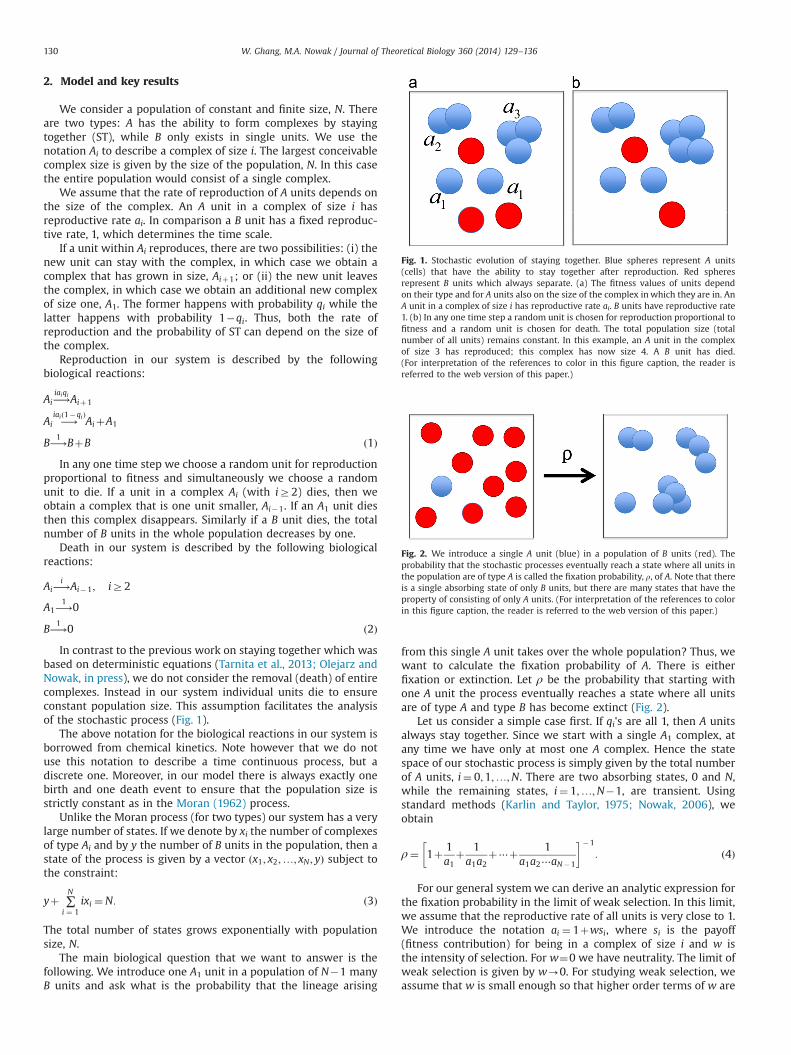
The main biological question that we want to answer is thefollowing. We introduce one A1 unit in a population of N�1 manyB units and ask what is the probability that the lineage arising

from this single A unit takes over the whole population? Thus, wewant to calculate the fixation probability of A. There is eitherfixation or extinction. Let ρ be the probability that starting withone A unit the process eventually reaches a state where all unitsare of type A and type B has become extinct (Fig. 2).

Let us consider a simple case first. If qi's are all 1, then A unitsalways stay together. Since we start with a single A1 complex, atany time we have only at most one A complex. Hence the statespace of our stochastic process is simply given by the total numberof A units, i¼ 0;1;…;N. There are two absorbing states, 0 and N,while the remaining states, i¼ 1;…;N�1, are transient. Usingstandard methods (Karlin and Taylor, 1975; Nowak, 2006), weobtain

ρ¼ 1þ 1a1

þ 1a1a2

þ⋯þ 1a1a2⋯aN�1

� ��1

: ð4Þ

For our general systemwe can derive an analytic expression forthe fixation probability in the limit of weak selection. In this limit,we assume that the reproductive rate of all units is very close to 1.We introduce the notation ai ¼ 1þwsi, where si is the payoff(fitness contribution) for being in a complex of size i and w isthe intensity of selection. For w¼0 we have neutrality. The limit ofweak selection is given by w-0. For studying weak selection, weassume that w is small enough so that higher order terms of w are

Fig. 1. Stochastic evolution of staying together. Blue spheres represent A units(cells) that have the ability to stay together after reproduction. Red spheresrepresent B units which always separate. (a) The fitness values of units dependon their type and for A units also on the size of the complex in which they are in. AnA unit in a complex of size i has reproductive rate ai. B units have reproductive rate1. (b) In any one time step a random unit is chosen for reproduction proportional tofitness and a random unit is chosen for death. The total population size (totalnumber of all units) remains constant. In this example, an A unit in the complexof size 3 has reproduced; this complex has now size 4. A B unit has died.(For interpretation of the references to color in this figure caption, the reader isreferred to the web version of this paper.)

Fig. 2. We introduce a single A unit (blue) in a population of B units (red). Theprobability that the stochastic processes eventually reach a state where all units inthe population are of type A is called the fixation probability, ρ, of A. Note that thereis a single absorbing state of only B units, but there are many states that have theproperty of consisting of only A units. (For interpretation of the references to colorin this figure caption, the reader is referred to the web version of this paper.)

W. Ghang, M.A. Nowak / Journal of Theoretical Biology 360 (2014) 129–136130

negligible. In this case, and retaining general qi, we obtain

ρ¼ 1NþN�1

2N∑N�1

i ¼ 1 Cisi∑N�1

i ¼ 1 Ciw ð5Þ

where

Ci ¼ ∏i�1

j ¼ 1ðN�1� jÞqj ∏

N�1

j ¼ iþ1ðNþ1� jqjÞ: ð6Þ

Therefore, the fixation of ST is favored by selection, ρ41=N, if

∑N�1

i ¼ 1Cisi40: ð7Þ

These results are proved in Appendices A and B.If the qi values are less than one, then the fitness contribution

of smaller complexes is more important than that of largercomplexes. Since Ciþ1=Ci ¼ ðN�1� iÞqi=ðNþ1�ðiþ1Þqiþ1Þ whichfor large N is approximately qi, the coefficient ðN�1Þ Ciþ1=

2N∑N�1i ¼ 1 Ci of siþ1 is qi times smaller than the coefficient

ðN�1ÞCi=2N∑N�1i ¼ 1 Ci of si. Hence, the fitness contributions of

smaller complexes are more important in determining the fixationof A.

It is plausible that in many biological settings, ST complexeshave a maximum size beyond which further growth is impossible.Let us now consider the case where 0oqir1 for all iok and qi¼0for all iZk. Thus, Ak is the largest complex that can be generated.There is no growth from Ak to Akþ1 and beyond. For weak selectionthe probability of fixation is given by

ρ¼ 1NþN�1

2N∑k

i ¼ 1Cisi∑k

i ¼ 1Ciw ð8Þ

where

Ci ¼ ðNþ1Þ ∏i�1

j ¼ 1ðN�1� jÞqj ∏

k�1

j ¼ iþ1ðNþ1� jqjÞ; i¼ 1;…; k�1 ð9Þ

and

Ck ¼ ∏k�1

j ¼ 1ðN�1� jÞqj ð10Þ

For large N, we have the following asymptotic expression for thefixation probability:

ρ¼ 1Nþw

s1þq1s2þq1q2s3þ⋯þq1q2⋯qk�1sk2ð1þq1þq1q2þ⋯þq1q2⋯qk�1Þ

þO1N

� �� �: ð11Þ

Therefore, the fixation of ST with maximum size k is favored byselection if

∑k

j ¼ 1sj ∏

j�1

i ¼ 1qi40 ð12Þ

This condition holds for large population size and weak selection.More generally, we can prove that if (11) holds then for any initialstate the fixation of A is favored by selection and the fixation of B isopposed by selection.

In the next section, we describe a method how to evaluate thefixation probabilities in our stochastic process.

3. Derivation of system of linear equations for fixationprobabilities

A state of our stochastic process is given by the pair ð x!; yÞ. Thevector x!¼ ðx1; x2;…; xNÞ denotes the configuration of the A unitsin the population. The nonnegative integer xi represents thenumber of complexes of size i. The largest possible complex hassize, N, which is the total population size. The nonnegative integery denotes the number of B units. Since the total population size is

strictly constant, we have the constraint

N¼ yþ ∑N

i ¼ 1ixi ð13Þ

We need to calculate the probabilities of all possible transitionsfrom state ð x!; yÞ. For this purpose, we introduce notations forbirth and death events. The probability that a unit within acomplex Ai is chosen for reproduction is given by

bi ¼iaixi

yþ∑Nj ¼ 1jajxj

ð14Þ

The probability that a B unit is chosen for reproduction is given by

b¼ yyþ∑N

j ¼ 1jajxjð15Þ

The probability that a unit within complex Ai is chosen for death is

di ¼ixiN

ð16Þ

The probability that a B is chosen for death is

d¼ yN

ð17Þ

In order to describe transitions in the system, we define the ithstandard unit vector ei ¼ ð0;…;0;1;0;…;0Þ where the ith compo-nent is 1 and all others are zero. Starting from a generic state,ð x!; yÞ, we have the following 10 transitions:

1. A unit in Ai is chosen for reproduction and its offspring stayswith the complex; a B unit is chosen for death. This eventhappens with probability bidqi. The transition is

ð x!; yÞ-ð x!þeiþ1�ei; y�1Þ: ð18Þ

2. A unit in Ai is chosen for reproduction and its offspring doesnot stay; a B unit is chosen for death. This event happens withprobability bidð1�qiÞ. The transition is

ð x!; yÞ-ð x!þe1; y�1Þ: ð19Þ

3. A unit in Ai is chosen for reproduction and its offspring stayswith the complex; a unit in the same Ai complex is chosen fordeath. This event happens with probability biði=NÞqi. The stateremains the same; the transition is

ð x!; yÞ-ð x!; yÞ: ð20Þ

4. A unit in Ai is chosen for reproduction and its offspring doesnot stay; a unit in the same Ai complex is chosen for death.This event happens with probability biði=NÞð1�qiÞ. The transi-tion is

ð x!; yÞ-ð x!�eiþei�1þe1; yÞ: ð21Þ

5. A unit in Ai is chosen for reproduction and its offspring stayswith the complex; a unit in a different Ai complex is chosen fordeath. This event happens with probability biðdi� i=NÞqi. Thetransition is

ð x!; yÞ-ð x!þeiþ1þei�1�2ei; yÞ: ð22Þ

6. A unit in Ai is chosen for reproduction and its offspringdoes not stay; a unit in different Ai complex is chosen fordeath. This event happens with probability biðdi� i=NÞð1�qiÞ.

W. Ghang, M.A. Nowak / Journal of Theoretical Biology 360 (2014) 129–136 131

The transition is

ð x!; yÞ-ð x!þe1þei�1�ei; yÞ: ð23Þ

7. A unit in Ai is chosen for reproduction and its offspring stayswith the complex; a unit in Aj (ja i) is chosen for death. Thisevent happens with probability bidjqi. The transition is

ð x!; yÞ-ð x!þeiþ1�ei�ejþej�1; yÞ: ð24Þ

8. A unit in Ai complex is chosen for reproduction and itsoffspring does not stay; a unit in Aj (ja i) is chosen for death.This event happens with the probability bidjð1�qiÞ. Thetransition is

ð x!; yÞ-ð x!þe1�ejþej�1; yÞ: ð25Þ

9. A B unit is chosen for reproduction; a unit in Ai is chosen fordeath. This event happens with the probability bdi. Thetransition is

ð x!; yÞ-ð x!�eiþei�1; yþ1Þ: ð26Þ

10. A B unit is chosen for reproduction; a B unit is chosen fordeath. This event happens with probability bd. The stateremains the same; the transition is

ð x!; yÞ-ð x!; yÞ: ð27Þ

As in the standard Moran (1962) process, we choose thebirth and death events at the same time to maintain exactly thesame number of individuals. Thus, the size of the population isalways constant, N, and the same for both types of events. Notealso that if the birth and death events occur in a complex of thesame size, then we must distinguish between whether it isexactly the same complex or another complex of the same size,because the two cases yield different transitions (as shownabove).

We denote by ρx!;y

the probability that A reaches fixationwhen starting from state ð x!; yÞ. A has reached fixation, if thepopulation is in a state of the form ð z!;0Þ, which means that B hasbecome extinct, y¼0. There are many states where A has becomefixed. All those states fulfill the constraint ∑N

i ¼ 1ixi ¼N. The otherabsorption possibility is that A becomes extinct and B reaches

fixation, y¼N. There is exactly one such state, which we denote byð 0!;NÞ.

The fixation probabilities are given by the following equation:

ρx!;y

¼∑ibidqiρ x!þ eiþ 1 �ei ;y�1

þ∑ibidð1�qiÞρ x!þe1 ;y�1

þ∑ibi

iNqiρ x!;y

þ∑ibi

iNð1�qiÞρ x!�ei þ ei� 1 þ e1 ;y

þ∑ibi di�

iN

� �qiρ x!þeiþ 1 þei� 1 �2ei ;y

þ∑ibi di�

iN

� �ð1�qiÞρ x!þe1 þ ei� 1 � ei ;y

þ∑ibi ∑

ja idjqiρ x!þ eiþ 1 � ei �ej þ ej� 1 ;y

þ∑ibi ∑

ja idjð1�qiÞρ x!þ e1 � ej þej� 1 ;y

þ∑ibdiρ x!�ei þ ei� 1 ;yþ1

þbdρx!;y

ð28Þ

The summation is always i¼ 1;…;N unless otherwise stated. The ρvalues satisfy the boundary conditions: ρ

0!

;N¼ 0 and ρ

z!;0¼ 1.

Using the above system of linear equations, we can computethe fixation probabilities, but the problem becomes quite intract-able even for moderate N, because of the large number of states.The number of transient states (with 0oyoN) is given bypð1Þþpð2Þþ⋯þpðN�1Þ, where p(i) is the ith partition number.Hardy and Ramanujan (1918) derived for large N that

pðNÞ � 14ffiffiffi3

pNexpðπ

ffiffiffiffiffiffiffiffiffiffiffiffi2N=3

pÞ: ð29Þ

Using the Stolz–Cesáro Theorem (Stolz, 1885; Cesáro, 1888), we canprove

pð1Þþpð2Þþ⋯þpðNÞ � 12π

ffiffiffiffiffiffiffi2N

p expðπffiffiffiffiffiffiffiffiffiffiffiffi2N=3

pÞ ð30Þ

which is the approximate number of transient states in ourprocess for large N. For example, if N¼100 there are about 1:5�109 transient states.

In the Appendix we show how to calculate analytical expres-sions for the fixation probabilities in the limit of weak selection,thereby providing a derivation of our main results that were listedin Section 2.

4. Conclusion

We have introduced a stochastic process to study the evolutionof staying together in populations of finite size. We have derived aspecial result for the case of any intensity of selection. We havederived general results for the limit of weak selection. Our mainresult is the following. Suppose that staying together generatescomplexes up to a maximum size, k, but not beyond. In this casewe have qi40 for i¼ 1;…; k�1 and qi¼0 for iZk. The reproduc-tive rate of a unit in a complex of size i is given by ai ¼ 1þwsi,where si is the selection coefficient and w is the intensity ofselection. For large population size, N, and in the limit of weakselection, w-0, we find that staying together is advantageous if

s1þq1s2þq1q2s3þ⋯þq1q2⋯qk�1sk40: ð31ÞWhat is the intuition for this result? First of all, we note that we

obtain a linear function in the fitness values, si, which is expectedgiven that we consider the limit of weak selection. Second, weobserve that the selection coefficients of smaller complexes are

0.0 0.2 0.4 0.6 0.8 1.00

50

100

150

Probablity to stay together, q

j 2

j 3

=

=

Crit

ical

ben

efit

to c

ost r

atio

, b/c

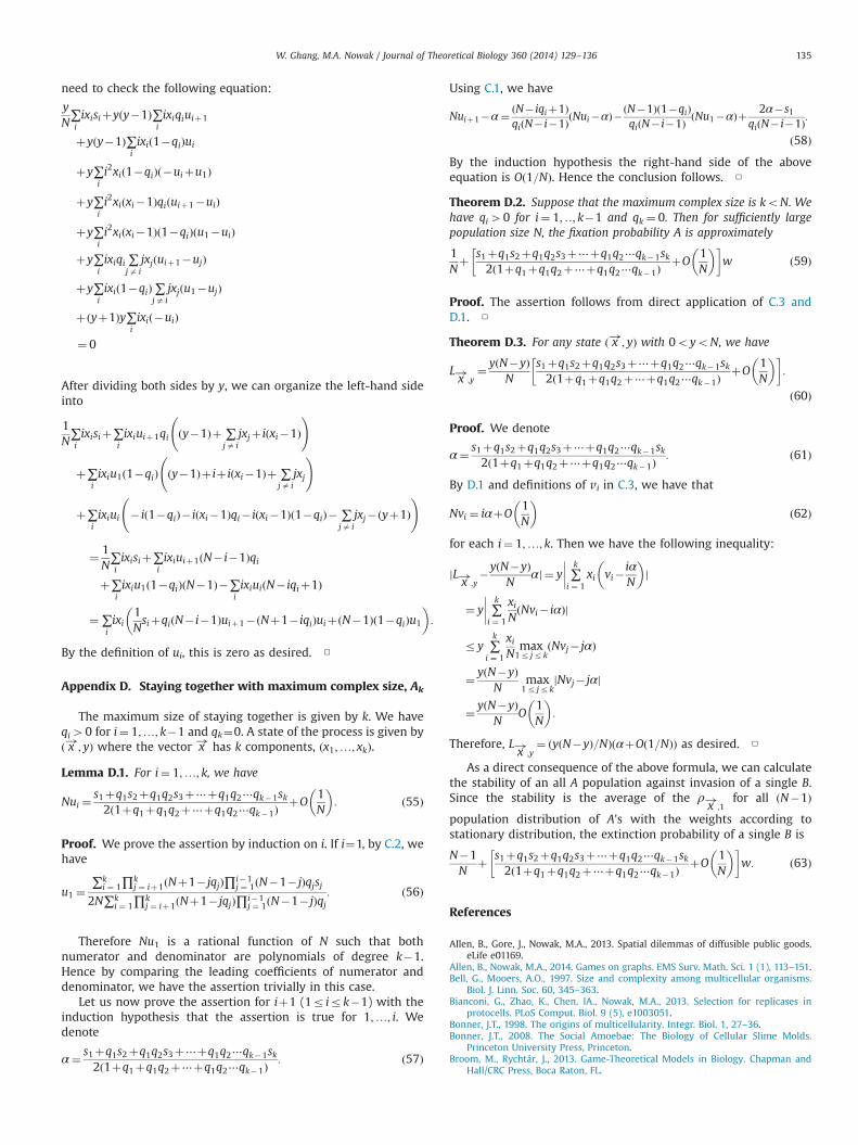
Fig. 3. The critical benefit to cost ratio, b/c, is shown as a function of the probabilityto stay together, q. The fitness landscape is given by si ¼ �c for i¼ 1;2;…; j andsi ¼ b�c for i¼ jþ1;…; k. The maximum complex size is k¼10. The minimum sizefor a beneficial complex is j¼2 (blue) or j¼3 (red). (For interpretation of thereferences to color in this figure caption, the reader is referred to the web version ofthis paper.)

W. Ghang, M.A. Nowak / Journal of Theoretical Biology 360 (2014) 129–136132

relatively more important than that of larger ones, which makessense given that larger complexes have to arise from smaller onesand are less abundant in the equilibrium distribution. Specifically,the selection coefficients of large complexes are discounted by theproducts of the probabilities of staying together describing thesequence of events that would form them. Note also that if allselection coefficients are zero, we have neutrality. If all selectioncoefficients are positive, then staying together is obviously favoredby selection. Interesting conditions emerge, if some selectioncoefficients are negative while others are positive.

Special cases of the above criterion are

(i) Let q1 ¼ q2 ¼⋯¼ qk�1 ¼ 1 and qk¼0. This means that there iscertainty of staying together up to size k, but not beyond.In this case, ST is advantageous if

s1þs2þ⋯þsk40: ð32Þ

(ii) Let qi ¼ qo1 and qk¼0. This means that there is a fixedprobability of staying together, which is the same for allcomplexes of size smaller than k. Once size k is reached allnew units leave with certainty. In this case, ST is advanta-geous if

s1þqs2þ⋯þqk�1sk40: ð33ÞWe can also consider particular choices for the fitnesslandscape.

(iia) Fitness landscape with step function (Fig. 3): si ¼ �c fori¼ 1;2;…; j and si ¼ b�c for i¼ jþ1;…; k. ST entails a cost.Complexes provide a benefit if they are greater than size j.Here ST is advantageous if

bc4

1�qk

qjð1�qk� jÞ: ð34Þ

(iib) Linear fitness slope (Fig. 4): si ¼ �cþbði�1Þ. Again ST entails acost, but complexes also provide benefits that increase linearlywith the size of the complex. Here ST is advantageous if

bc4

ð1�qÞð1�qkÞqð1þðk�1Þqk�kqk�1Þ

: ð35Þ

Subsequent work on stochastic staying together might incor-porate diffusible public goods (Allen et al., 2013; Olejarz andNowak, in press), evolutionary game dynamics in populations of

finite size (Nowak et al., 2004; Imhof and Nowak, 2006; Lessardand Ladret, 2007; Ladret and Lessard, 2008), and spatial selection(Nowak and May, 1992; Killingback and Doebeli, 1996, 1998; vanBaalen and Rand, 1998; Szabó and Hauert, 2002; Hauert andDoebeli, 2004; Ifti et al., 2004; Santos and Pacheco, 2005; Szabóand Fath, 2007; Gore et al., 2009; Tarnita et al., 2009; Nowak et al.,2010b; Damore and Gore, 2012; Garcia and De Monte, 2012;Broom and Rychtár, 2013; Sanchez and Gore, 2013; Allen andNowak, 2014). We are also interested in characterizing themutation-selection distribution of different ST mutants over allpossible transient states.

Appendix A. The limit of weak selection

We can derive analytical results in the limit of weak selection.Let us write the fitness value of an A unit in a complex Ai as

ai ¼ 1þwsi: ð36Þ

The parameter w scales the intensity of selection. The value si isthe selection coefficient that is associated with being in a complexof size i. As before the fitness value of B units is 1. The limit of weakselection is given by w-0. In particular, we can write Taylorexpansions keeping linear terms in w and neglecting higherorder terms.

For complete neutrality, w¼0, each unit is equally likely toproduce a lineage which will be inherited by the entire population.Therefore, we have

ρx!;y

¼N�yN

: ð37Þ

For the limit of weak selection, adding linear terms in w, thefixation probabilities must be of the form

ρx!;y

�N�yN

þwLx!;y

: ð38Þ

The linear terms, Lx!;y

, can be calculated by plugging these fixationprobabilities into system (28). We obtain

N2Lx!;y

¼ yN∑iixisi

þy∑iixiqiL x!þ eiþ 1 � ei ;y�1

þy∑iixið1�qiÞL x!þ e1 ;y�1

þ∑ii2xiqiL x!;y

þ∑ii2xið1�qiÞL x!� ei þei� 1 þe1 ;y

þ∑ii2xiðxi�1ÞqiL x!þ eiþ 1 þ ei� 1 �2ei ;y

þ∑ii2xiðxi�1Þð1�qiÞL x!þ e1 þ ei� 1 �ei ;y

þ∑iixiqi ∑

ja ijxjL x!þ eiþ 1 � ei �ej þ ej� 1 ;y

þ∑iixið1�qiÞ∑

ja ijxjL x!þ e1 � ej þej� 1 ;y

þy∑iixiL x!� ei þei� 1 ;yþ1

þy2Lx!;y

ð39Þ

The L terms satisfy the boundary conditions L0!

;N¼ 0 and

Lz!;0

¼ 1 for all vector z!'s. Although the system still contains

exponentially many variables, we can solve it explicitly. Let usintroduce the sequence of numbers u1;u2;…;uN�1. We start with

0.0 0.2 0.4 0.6 0.8 1.00

2

4

6

8

10

Probablity to stay together, q

k 3

k 100

=

=

Crit

ical

ben

efit

to c

ost r

atio

, b/c

Fig. 4. The critical benefit to cost ratio, b/c, is shown as a function of the probabilityto stay together, q. The fitness landscape is given by si ¼ �cþbði�1Þ for i¼ 1;…; k.The maximum complex size is k¼3 (blue) or k¼100 (red). (For interpretation of thereferences to color in this figure caption, the reader is referred to the web version ofthis paper.)

W. Ghang, M.A. Nowak / Journal of Theoretical Biology 360 (2014) 129–136 133

the definition

u1 ¼∑N�1

i ¼ 1∏i�1j ¼ 1ðN�1� jÞqj∏N�1

j ¼ iþ1ðNþ1� jqjÞsi2N∑N�1

i ¼ 1∏i�1j ¼ 1ðN�1� jÞqj∏N�1

j ¼ iþ1ðNþ1� jqjÞ: ð40Þ

We define uiþ1 for i¼ 1;…;N�2 inductively as follows:

qiðN� i�1Þuiþ1 ¼ ðN� iqiþ1Þui�ðN�1Þð1�qiÞu1�si=N ð41ÞWe introduce the summation sequence vi ¼ u1þ⋯þui for

i¼ 1;…;N�1. Then we construct the vector v! whose ith coordi-nate is vi. Now we are ready to present the exact solution as

Lx!;y

¼ y x!� v!: ð42Þ

This result can be proven by direct computation. See Appendix Cfor details.

The fixation probability of a single A unit is

ρ¼ ρe1 ;N�1 ¼1NþwLe1 ;N�1: ð43Þ

Remember that e1 is the N-dimensional vector ð1;0;…;0Þ. Weobtain

ρ¼ 1NþN�1

2N∑N�1

i ¼ 1 Cisi∑N�1

i ¼ 1 Ciw ð44Þ

where

Ci ¼ ∏i�1

j ¼ 1ðN�1� jÞqj ∏

N�1

j ¼ iþ1ðNþ1� jqjÞ: ð45Þ

This result holds for the limit of weak selection. Note that thecontribution of the selection coefficient si to the fixation prob-ability, ρ, is ½Nþ1�ðiþ1Þqiþ1�=½ðN�1� iÞqi� times larger than thatof siþ1. For large N the impact of si is 1=qi times larger than theimpact of siþ1. Thus, for qi values less than one, we find that thefitness contributions of smaller complexes are more importantthan that of larger complexes, which makes sense.

Appendix B. Weak selection and maximum complex size

We now introduce a maximum complex size, k. It is possible togrow up to Ak, but not beyond. If a unit in Ak is chosen forreproduction, the offspring will always leave. Therefore qi40 forall i¼ 1;‥; k�1, but qk¼0. A state of our system is again given byð x!; yÞ, but the vector x! has only k many componentsðx1; x2;…; xkÞ. We derive a simple criterion for A to be advanta-geous or disadvantageous, which holds for large population size,N. Consider the quantity

C ¼ ∑k

j ¼ 1sj ∏

j�1

i ¼ 1qi: ð46Þ

If C40 then for any initial state ð x!; yÞ we have ρð x!;yÞ

4 ðN�yÞ=N,which means that the fixation of A is favored by selection starting

from any initial state. If Co0 then for any initial state ð x!; yÞ wehave ρ

ð x!;yÞoðN�yÞ=N, which means that the fixation of A is

opposed by selection starting from any initial state.Using Eq. (44) for ρe1 ;N�1, we have

ρe1 ;N�1 �1NþN�1

2NC1s1þC2s2þ⋯þCksk

C1þC2þ⋯þCkw ð47Þ

where

Ci ¼ ðNþ1Þ ∏i�1

j ¼ 1ðN�1� jÞqj ∏

k�1

j ¼ iþ1ðNþ1� jqjÞ; 8 i¼ 1;…; k�1

ð48Þ

and

Ck ¼ ðN�2ÞðN�3Þ⋯ðN�kÞq1q2⋯qk�1: ð49ÞFurthermore, we can derive

ρx!;y

¼N�yN

þyðN�yÞN

s1þq1s2þq1q2s3þ⋯þq1q2⋯qk�1sk2ð1þq1þq1q2þ⋯þq1q2⋯qk�1Þ

�

þO1N

� ��w ð50Þ

for any transient initial state ð x!; yÞ. The proof is presented inAppendix D.

Appendix C. Proof of formula Lx!;y

¼ y x!� v!

Lemma C.1. The system of linear equations

1NsiþqiðN� i�1Þuiþ1�ðN� iqiþ1ÞuiþðN�1Þð1�qiÞu1 ¼ 0 ð51Þ

with i¼ 1;…;N�1 has a unique solution. For convention, we assumeuN ¼ 0.

Proof. We show that the corresponding matrix is non-singular.Let t

!be an arbitrary null vector of the matrix. In other words, the

components ti satisfy

qiðN� i�1Þtiþ1�ðN� iqiþ1ÞtiþðN�1Þð1�qiÞt1 ¼ 0 ð52Þfor i¼ 1;…;N�1. Let M be the maximum modulus of t

!and it is

attained at 1r jrN�1. Hence M¼ jtjj. By the triangle inequality,we have

ðN� jqjþ1ÞM¼ ðN� iqiþ1Þjujj¼ jqjðN� j�1Þtjþ1þðN�1Þð1�qjÞt1jr jqjðN� j�1Þtjþ1jþjðN�1Þð1�qjÞt1jrqjðN� j�1ÞMþðN�1Þð1�qjÞM¼ ðN� jqj�1ÞM:

Therefore M¼0 and ti's are all zeros. Therefore 0!

is the only nullvector of the corresponding matrix and hence the matrix is non-singular, as desired. □

Lemma C.2. In the solution of the above system in C.1, we have

u1 ¼∑N�1

i ¼ 1∏N�1j ¼ iþ1ðNþ1� jqjÞ∏i�1

j ¼ 1ðN�1� jÞqjsi2N∑N�1

i ¼ 1∏N�1j ¼ iþ1ðNþ1� jqjÞ∏i�1

j ¼ 1ðN�1� jÞqjð53Þ

Proof. This can be proved by observing the following identity:

1N

∑N�1

i ¼ 1∏i�1

j ¼ 1ðN�1� jÞqj ∏

N�1

j ¼ iþ1ðNþ1� jqjÞsj

¼ ∑N�1

i ¼ 1∏i�1

j ¼ 1ðN�1� jÞqj ∏

N�1

j ¼ iþ1ðNþ1� jqjÞððN� iqiþ1Þui

�qiðN� i�1Þuiþ1�ðN�1Þð1�qiÞu1Þ

Note that all the ui terms are cancelled for iZ2. □

Theorem C.3. For each population N, there exists a RN�1 vector v!which only depends linearly on si's and depends on N and qi's suchthat

Lx!;y

¼ y x!� v! ð54Þ

for any population N, i.e, yþ∑N�1i ¼ 1 ixi ¼N. The vi's are given by

vi ¼ u1þu2þ⋯þui for each i¼ 1;…N�1 where ui's are solution ofthe system of linear equations in C.1.

Proof. We need to show that Lx!;y

¼ y x!� v! is a solution bydirectly plugging it into (39). After cancelling x!� v! terms, we

W. Ghang, M.A. Nowak / Journal of Theoretical Biology 360 (2014) 129–136134

need to check the following equation:

yN∑iixisiþyðy�1Þ∑

iixiqiuiþ1

þyðy�1Þ∑iixið1�qiÞui

þy∑ii2xið1�qiÞð�uiþu1Þ

þy∑ii2xiðxi�1Þqiðuiþ1�uiÞ

þy∑ii2xiðxi�1Þð1�qiÞðu1�uiÞ

þy∑iixiqi ∑

ja ijxjðuiþ1�ujÞ

þy∑iixið1�qiÞ∑

ja ijxjðu1�ujÞ

þðyþ1Þy∑iixið�uiÞ

¼ 0

After dividing both sides by y, we can organize the left-hand sideinto

1N∑iixisiþ∑

iixiuiþ1qi ðy�1Þþ ∑

ja ijxjþ iðxi�1Þ

!

þ∑iixiu1ð1�qiÞ ðy�1Þþ iþ iðxi�1Þþ ∑

ja ijxj

!

þ∑iixiui � ið1�qiÞ� iðxi�1Þqi� iðxi�1Þð1�qiÞ� ∑

ja ijxj�ðyþ1Þ

!

¼ 1N∑iixisiþ∑

iixiuiþ1ðN� i�1Þqi

þ∑iixiu1ð1�qiÞðN�1Þ�∑

iixiuiðN� iqiþ1Þ

¼∑iixi

1NsiþqiðN� i�1Þuiþ1�ðNþ1� iqiÞuiþðN�1Þð1�qiÞu1

� �:

By the definition of ui, this is zero as desired. □

Appendix D. Staying together with maximum complex size, Ak

The maximum size of staying together is given by k. We haveqi40 for i¼ 1;…; k�1 and qk¼0. A state of the process is given byð x!; yÞ where the vector x! has k components, ðx1;…; xkÞ.

Lemma D.1. For i¼ 1;…; k, we have

Nui ¼s1þq1s2þq1q2s3þ⋯þq1q2⋯qk�1sk2ð1þq1þq1q2þ⋯þq1q2⋯qk�1Þ

þO1N

� �: ð55Þ

Proof. We prove the assertion by induction on i. If i¼1, by C.2, wehave

u1 ¼∑k

i ¼ 1∏kj ¼ iþ1ðNþ1� jqjÞ∏i�1

j ¼ 1ðN�1� jÞqjsj2N∑k

i ¼ 1∏kj ¼ iþ1ðNþ1� jqjÞ∏i�1

j ¼ 1ðN�1� jÞqj: ð56Þ

Therefore Nu1 is a rational function of N such that bothnumerator and denominator are polynomials of degree k�1.Hence by comparing the leading coefficients of numerator anddenominator, we have the assertion trivially in this case.

Let us now prove the assertion for iþ1 (1r irk�1) with theinduction hypothesis that the assertion is true for 1;…; i. Wedenote

α¼ s1þq1s2þq1q2s3þ⋯þq1q2⋯qk�1sk2ð1þq1þq1q2þ⋯þq1q2⋯qk�1Þ

: ð57Þ

Using C.1, we have

Nuiþ1�α¼ ðN� iqiþ1ÞqiðN� i�1ÞðNui�αÞ�ðN�1Þð1�qiÞ

qiðN� i�1Þ ðNu1�αÞþ 2α�s1qiðN� i�1Þ:

ð58ÞBy the induction hypothesis the right-hand side of the aboveequation is Oð1=NÞ. Hence the conclusion follows. □

Theorem D.2. Suppose that the maximum complex size is koN. Wehave qi40 for i¼ 1;‥; k�1 and qk ¼ 0. Then for sufficiently largepopulation size N, the fixation probability A is approximately

1Nþ s1þq1s2þq1q2s3þ⋯þq1q2⋯qk�1sk

2ð1þq1þq1q2þ⋯þq1q2⋯qk�1ÞþO

1N

� �� �w ð59Þ

Proof. The assertion follows from direct application of C.3 andD.1. □

Theorem D.3. For any state ð x!; yÞ with 0oyoN, we have

Lx!;y

¼ yðN�yÞN

s1þq1s2þq1q2s3þ⋯þq1q2⋯qk�1sk2ð1þq1þq1q2þ⋯þq1q2⋯qk�1Þ

þO1N

� �� �:

ð60Þ

Proof. We denote

α¼ s1þq1s2þq1q2s3þ⋯þq1q2⋯qk�1sk2ð1þq1þq1q2þ⋯þq1q2⋯qk�1Þ

: ð61Þ

By D.1 and definitions of vi in C.3, we have that

Nvi ¼ iαþO1N

� �ð62Þ

for each i¼ 1;…; k. Then we have the following inequality:

jLx!;y

�yðN�yÞN

αj ¼ y ∑k

i ¼ 1xi vi�

iαN

� �j

����¼ y ∑

k

i ¼ 1

xiNðNvi� iαÞj

����ry ∑

k

i ¼ 1

xiN

max1r jrk

ðNvj� jαÞ

¼ yðN�yÞN

max1r jrk

jNvj� jαj

¼ yðN�yÞN

O1N

� �:

Therefore, Lx!;y

¼ ðyðN�yÞ=NÞðαþOð1=NÞÞ as desired. □

As a direct consequence of the above formula, we can calculatethe stability of an all A population against invasion of a single B.Since the stability is the average of the ρ

x!;1for all ðN�1Þ

population distribution of A's with the weights according tostationary distribution, the extinction probability of a single B is

N�1N

þ s1þq1s2þq1q2s3þ⋯þq1q2⋯qk�1sk2ð1þq1þq1q2þ⋯þq1q2⋯qk�1Þ

þO1N

� �� �w: ð63Þ

References

Allen, B., Gore, J., Nowak, M.A., 2013. Spatial dilemmas of diffusible public goods.eLife e01169.

Allen, B., Nowak, M.A., 2014. Games on graphs. EMS Surv. Math. Sci. 1 (1), 113–151.Bell, G., Mooers, A.O., 1997. Size and complexity among multicellular organisms.

Biol. J. Linn. Soc. 60, 345–363.Bianconi, G., Zhao, K., Chen, IA., Nowak, M.A., 2013. Selection for replicases in

protocells. PLoS Comput. Biol. 9 (5), e1003051.Bonner, J.T., 1998. The origins of multicellularity. Integr. Biol. 1, 27–36.Bonner, J.T., 2008. The Social Amoebae: The Biology of Cellular Slime Molds.

Princeton University Press, Princeton.Broom, M., Rychtár, J., 2013. Game-Theoretical Models in Biology. Chapman and

Hall/CRC Press, Boca Raton, FL.

W. Ghang, M.A. Nowak / Journal of Theoretical Biology 360 (2014) 129–136 135

Carroll, S.B., 2001. Chance and necessity: the evolution of morphological complexityand diversity. Nature 409, 1102–1109.

Cesáro, E., 1888. Sur la convergence des séries, Nouvelles annales de mathéma-tiques Series 3, 7, 49–59.

Chen, I.A., Salehi-Ashtiani, K., Szostak, J.W., 2005. RNA catalysis in model protocellvesicles. J. Am. Chem. Soc. 127, 13213–13219.

Damore, J.A., Gore, J., 2012. Understanding microbial cooperation. J. Theor. Biol. 299,31–41.

Furusawa, C., Kaneko, K., 2000. Complex organization in multicellularity as anecessity in evolution. Artif. Life 6, 265–281.

Gadagkar, R., 1994. Social insects and social amoebae. J. Biosci. 19, 219–245.Gadagkar, R., 2001. The Social Biology of Ropalidia marginata: Toward Under-

standing the Evolution of Eusociality. Harvard University Press, Cambridge.Garcia, T., De Monte, S., 2012. Group formation and the evolution of sociality.

Evolution 67, 131–141.Gore, J., Youk, H., Van Oudenaarden, A., 2009. Snowdrift game dynamics and

facultative cheating in yeast. Nature 459, 253–256.Grosberg, R.K., Strathmann, R.R., 2007. The evolution of multicellularity: a minor

major transition?. Annu. Rev. Ecol. Evol. Syst. 38, 621–654.Hardy, G.H., Ramanujan, S., 1918. Asymptotic formulae in combinatory analysis.

Proc. Lond. Math. Soc. 17, 75–115.Hauert, C., Doebeli, M., 2004. Spatial structure often inhibits the evolution of

cooperation in the snowdrift game. Nature 428, 643–646.Hölldobler, B., Wilson, E.O., 2009. The Superorganism: The Beauty, Elegance, and

Strangeness of Insect Societies. W.W. Norton, London.Hunt, J.H., 2007. The Evolution of Social Wasps. Oxford University Press, New York.Ifti, M., Killingback, T., Doebeli, M., 2004. Effects of neighbourhood size and

connectivity on the spatial Continuous Prisoner's Dilemma. J. Theor. Biol. 231,97–106.

Imhof, L.A., Nowak, M.A., 2006. Evolutionary game dynamics in a Wright–Fisherprocess. J. Math. Biol. 52 (5), 667–681.

Karlin, S., Taylor, H., 1975. A First Course in Stochastic Processes. Academic Press,San Diego.

Killingback, T., Doebeli, M., 1996. Spatial evolutionary game theory: Hawks andDoves revisited. Proc. R. Soc. B. 263, 1135–1144.

Killingback, T., Doebeli, M., 1998. Self-organized criticality in spatial evolutionarygame theory. J. Theor. Biol. 191, 335–340.

King, N., 2004. The unicellular ancestry of animal development. Dev. Cell 7,313–325.

Kirk, D.L., 2003. Seeking the ultimate and proximate causes of Volvox multi-cellularity and cellular differentiation. Integr. Comput. Biol. 43, 247–253.

Kirk, D.L., 2005. A twelve-step program for evolving multicellularity and a divisionof labor. BioEssays 27, 299–310.

Kolter, R., 2010. Biofilms in lab and nature: a molecular geneticist's voyage tomicrobial ecology. Int. Microbiol. 13, 1–7.

Koschwanez, J.H., Foster, K.R., Murray, A.W., 2011. Sucrose utilization in buddingyeast as a model for the origin of undifferentiated multicellularity. PLoS Biol.9 (8), e1001122.

Ladret, V., Lessard, S., 2008. Evolutionary game dynamics in a finite asymmetrictwo-deme population and emergence of cooperation. J. Theor. Biol. 255 (1),137–151.

Lessard, S., Ladret, V., 2007. The probability of fixation of a single mutant in anexchangeable selection model. J. Math. Biol. 54 (5), 721–744.

Margulis, L., 1981. Symbiosis in Cell Evolution. Life and its Environment on the EarlyEarth. Freeman, San Francisco.

Maynard Smith, J., Szathmary, E., 1998. The Major Transition in Evolution. OxfordUniversity Press, Oxford.

Michod, R.E., 1999. Darwinian Dynamics: Evolutionary Transitions in Fitness andIndividuality. Princeton University Press, Princeton.

Michod, R.E., 2007. Evolution of individuality during the transition from unicellularto multicellular life. Proc. Natl. Acad. Sci. USA 104, 8613–8618.

Moran, P.A.P., 1962. The Statistical Processes of Evolutionary Theory. ClarendonPress, Oxford.

Norman, T.M., Lord, N.D., Paulsson, J., Losick, R., 2013. Memory and modularity incell-fate decision making. Nature 503, 481–486.

Nowak, M.A., May, R.M., 1992. Evolutionary games and spatial chaos. Nature 359,826–829.

Nowak, M.A., Sasaki, A., Taylor, C., Fudenberg, D., 2004. Emergence of cooperationand evolutionary stability in finite populations. Nature 428, 646–650.

Nowak, M.A., 2006. Evolutionary Dynamics. Harvard University Press, Cambridge,Massachusetts, USA.

Nowak, M.A., Tarnita, C.E., Wilson, E.O., 2010a. The evolution of eusociality. Nature466, 1057–1062.

Nowak, M.A., Tarnita, C.E., Antal, T., 2010b. Evolutionary dynamics in structuredpopulations. Phil. Trans. R. Soc. B 365, 19–30.

Olejarz, J., Nowak, M.A.. Evolution of staying together in the context of diffusiblepublic goods. J. Theor. Biol., http://dx.doi.org/10.1016/j.jtbi.2014.06.023, inpress.

Pfeiffer, T., Bonhoeffer, S., 2003. An evolutionary scenario for the transition toundifferentiated multicellularity. Proc. Natl. Acad. Sci. 100, 1095–1098.

Rainey, P.B., 2007. Unity from conflict. Nature 446, 616.Ratcliff, W.C., Denison, R.F., Borrello, M., Travisano M., 2012. Experimental evolution

of multicellularity. Proc. Natl. Acad. Sci. 109 (5), 1595–1600.Ratcliff, W.C., Herron, M.D., Howell, K., Pentz, J.T., Rosenzweig, F., Travisano, M.,

2013. Experimental evolution of an alternating uni-and multicellular life cyclein Chlamydomonas reinhardtii. Nat. Commun. 4, 2742.

Rossetti, V., Schirrmeister, B.E., Bernasconi, M.V., Bagheri, H.C., 2010. The evolu-tionary path to terminal differentiation and division of labor in cyanobacteria.J. Theor. Biol. 262, 23–34.

Rossetti, V., Filippini, M., Svercel, M., Barbour, A.D., Bagheri, H.C., 2011. Emergentmulticellular life cycles in filementous bacteria owing to density-dependentpopulation dynamics. J. R. Soc. Interface 8, 1772–1784.

Sanchez, A., Gore, J., 2013. Feedback between population and evolutionarydynamics determines the fate of social microbial populations. PLoS Biol. 11 (4),e1001547.

Santos, F.C., Pacheco, J.M., 2005. Scale-free networks provide a unifying frameworkfor the emergence of cooperation. Phys. Rev. Lett. 95, 098104.

Stolz, O., 1885. Vorlesungen ueber allgemeine Arithmetik: nach den NeuerenAnsichten, Teubners, Leipzig, pp. 173–175.

Szabó, G., Hauert, C., 2002. Phase transitions and volunteering in spatial publicgoods games. Phys. Rev. Lett. 89, 118101.

Szabó, G., Fath, G., 2007. Evolutionary games on graphs. Phys. Rep. 446, 97–216.Tarnita, C.E., Ohtsuki, H., Antal, T., Fu, F., Nowak, M.A., 2009. Strategy selection in

structured populations. J. Theor. Biol. 259, 570–581.Tarnita, C.H., Taubes, C.H., Nowak, M.A., 2013. Evolutionary construction by staying

together and coming together. J. Theor. Biol. 320, 10–22.van Baalen, M., Rand, D.A., 1998. The unit of selection in viscous populations and

the evolution of altruism. J. Theor. Biol. 193 (4), 631–648.Willensdorfer, M., 2008. Organism size promotes the evolution of specialized cells

in multicellular digital organisms. J. Evol. Biol. 21, 104–110.Wilson, E.O., 1971. The Insect Societies. Harvard University Press, Cambridge.

W. Ghang, M.A. Nowak / Journal of Theoretical Biology 360 (2014) 129–136136