Stochastic and worst-case shape

optimization problems

Giuseppe Buttazzo

Dipartimento di Matematica

Universita di Pisa

buttazzo@dm.unipi.it

http://cvgmt.sns.it

“New Trends in Control Theory and PDEs”Roma, July 3–7, 2017

On the occasion of the 60th birthday of Piermarco Cannarsa

Bedlewo 2008 - social dinner

Benasque 2013 - excursion

Benasque 2013 - welcome reception

Joint works

• J.C. Bellido, G. Buttazzo, B. Velichkov: Worst-

case shape optimization for the Dirichlet en-

ergy. Nonlinear Analysis (2017).

• G. Buttazzo, B. Velichkov: A shape optimal

control problem and its probabilistic coun-

terpart. Paper submitted.

• G. Buttazzo, F. Maestre, B. Velichkov: Op-

timal potentials for problems with changing

sign data. Paper in preparation.

4

Jose Carlos Bellido (Universidad de Castilla-La Mancha, Spain)

Giuseppe Buttazzo (Universita di Pisa, Italy)

Faustino Maestre Caballero (Universidad deSevilla, Spain)

Bozhidar Velichkov (Universite de Grenoble,France)

papers available at:http://cvgmt.sns.it

http://arxiv.org

5

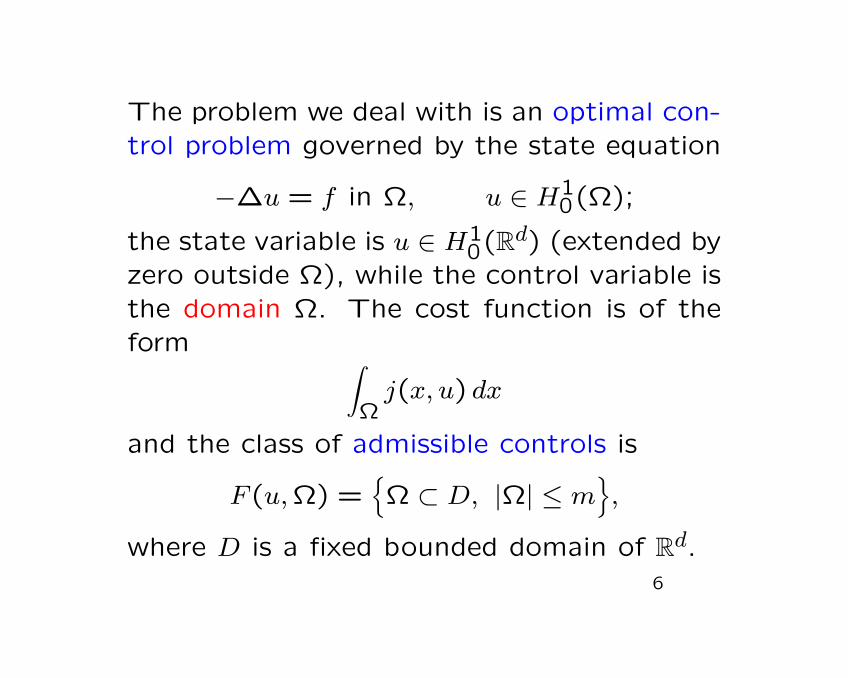
The problem we deal with is an optimal con-trol problem governed by the state equation

−∆u = f in Ω, u ∈ H10(Ω);

the state variable is u ∈ H10(Rd) (extended by

zero outside Ω), while the control variable isthe domain Ω. The cost function is of theform ∫

Ωj(x, u) dx

and the class of admissible controls is

F (u,Ω) =

Ω ⊂ D, |Ω| ≤ m,

where D is a fixed bounded domain of Rd.6

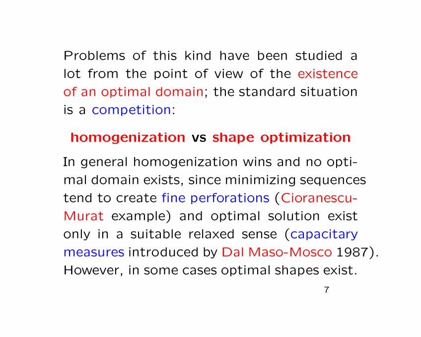
Problems of this kind have been studied a

lot from the point of view of the existence

of an optimal domain; the standard situation

is a competition:

homogenization vs shape optimization

In general homogenization wins and no opti-

mal domain exists, since minimizing sequences

tend to create fine perforations (Cioranescu-

Murat example) and optimal solution exist

only in a suitable relaxed sense (capacitary

measures introduced by Dal Maso-Mosco 1987).

However, in some cases optimal shapes exist.

7

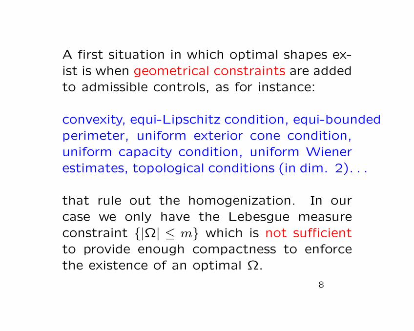
A first situation in which optimal shapes ex-ist is when geometrical constraints are addedto admissible controls, as for instance:

convexity, equi-Lipschitz condition, equi-boundedperimeter, uniform exterior cone condition,uniform capacity condition, uniform Wienerestimates, topological conditions (in dim. 2). . .

that rule out the homogenization. In ourcase we only have the Lebesgue measureconstraint |Ω| ≤ m which is not sufficientto provide enough compactness to enforcethe existence of an optimal Ω.

8

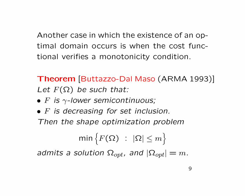
Another case in which the existence of an op-

timal domain occurs is when the cost func-

tional verifies a monotonicity condition.

Theorem [Buttazzo-Dal Maso (ARMA 1993)]

Let F (Ω) be such that:

• F is γ-lower semicontinuous;

• F is decreasing for set inclusion.

Then the shape optimization problem

minF (Ω) : |Ω| ≤ m

admits a solution Ωopt, and |Ωopt| = m.

9

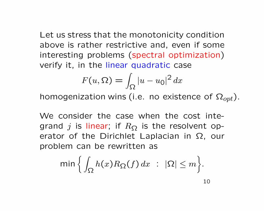
Let us stress that the monotonicity conditionabove is rather restrictive and, even if someinteresting problems (spectral optimization)verify it, in the linear quadratic case

F (u,Ω) =∫

Ω|u− u0|2 dx

homogenization wins (i.e. no existence of Ωopt).

We consider the case when the cost inte-grand j is linear; if RΩ is the resolvent op-erator of the Dirichlet Laplacian in Ω, ourproblem can be rewritten as

min ∫

Ωh(x)RΩ(f) dx : |Ω| ≤ m

.

10

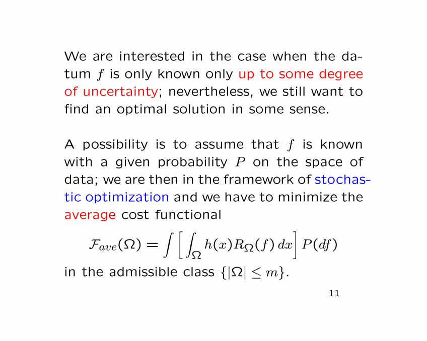
We are interested in the case when the da-tum f is only known only up to some degreeof uncertainty; nevertheless, we still want tofind an optimal solution in some sense.

A possibility is to assume that f is knownwith a given probability P on the space ofdata; we are then in the framework of stochas-tic optimization and we have to minimize theaverage cost functional

Fave(Ω) =∫ [ ∫

Ωh(x)RΩ(f) dx

]P (df)

in the admissible class |Ω| ≤ m.11

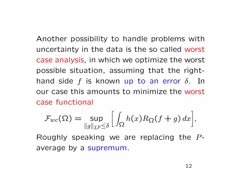
Another possibility to handle problems with

uncertainty in the data is the so called worst

case analysis, in which we optimize the worst

possible situation, assuming that the right-

hand side f is known up to an error δ. In

our case this amounts to minimize the worst

case functional

Fwc(Ω) = sup‖g‖Lp≤δ

[ ∫Ωh(x)RΩ(f + g) dx

],

Roughly speaking we are replacing the P -

average by a supremum.

12

Stochastic shape optimization

We want to determine the shape of a thermicconductor of a given measure m which mini-mizes the energy, but we only know the heatsources f up to a probability P on L2(Rd).We have then the problem

min ∫

E(Ω, f) dP (f) : |Ω| ≤ m

where

E(Ω, f) = minu∈H1

0(Ω)

∫Ω

(1

2|∇u|2 − fu

)dx.

This problems admits an optimal shape.

13

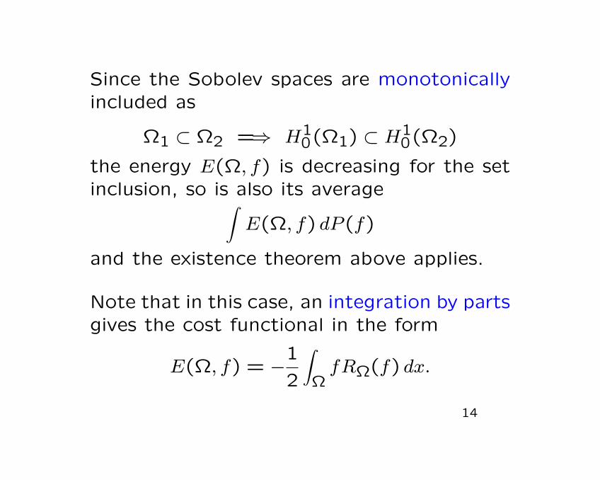
Since the Sobolev spaces are monotonicallyincluded as

Ω1 ⊂ Ω2 =⇒ H10(Ω1) ⊂ H1

0(Ω2)

the energy E(Ω, f) is decreasing for the setinclusion, so is also its average∫

E(Ω, f) dP (f)

and the existence theorem above applies.

Note that in this case, an integration by partsgives the cost functional in the form

E(Ω, f) = −1

2

∫ΩfRΩ(f) dx.

14

A more interesting (and realistic) situationis when the cost functional is perfectly de-termined and the uncertainty occurs only inthe PDE. the problem is then

min|Ω|≤m

∫ [ ∫Ωh(x)uΩ,f dx

]dP (f)

where the function h is perfectly known, whilethe heat source f is only known up the prob-ability P .

For instance, we want to maximize the av-erage temperature (i.e. h = 1) varying thedomain Ω, under only a partial informationabout the heat sources f .

15

Using the fact that the resolvent operator

RΩ is self-adjoint, we have, denoting by BPthe barycenter of P∫dP (f)

∫ΩhRΩ(f) dx =

∫dP (f)

∫ΩRΩ(h)f dx

=∫

ΩRΩ(h)

( ∫fdP (f)

)dx =

∫ΩRΩ(h)BP dx.

Notice that, by the maximum principle, the

monotonicity occurs when

BP ≥ 0 and h ≤ 0 or BP ≤ 0 and h ≥ 0.

16

Handling this case is rather more difficult(Buttazzo-Velichkov arxiv 2017), when thefunctions h and BP may change sign. Never-theless the existence of an optimal shape stillholds, together with some necessary condi-tions of optimality.

In this case, if the admissible class of do-mains is |Ω| ≤ m, in general we shouldnot expect the optimal domain Ωopt satu-rates the constraint. In fact, one of the op-timality conditions gives

either |Ωopt| = m or Ωopt ⊃ hBP ≤ 0.

17

Worst-case shape optimization

We deal here with the case when the controlis a domain; other cases of worst case op-timization problems can be found in Allaire-Dapogny (M3AS 2014). We want to showthe existence of an optimal domain for

minFwc(Ω) : Ω ⊂ D, |Ω| ≤ m

where Fwc is the worst-case functional

Fwc(Ω) = sup‖g‖Lp≤δ

[ ∫Ωh(x)RΩ(f + g) dx

],

Again, in general the cost Fwc(Ω) is not de-creasing with respect to the set inclusion.

18

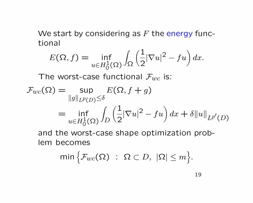
We start by considering as F the energy func-tional

E(Ω, f) = infu∈H1

0(Ω)

∫Ω

(1

2|∇u|2 − fu

)dx.

The worst-case functional Fwc is:

Fwc(Ω) = sup‖g‖Lp(D)≤δ

E(Ω, f + g)

= infu∈H1

0(Ω)

∫D

(1

2|∇u|2 − fu

)dx+ δ‖u‖

Lp′(D)

and the worst-case shape optimization prob-lem becomes

minFwc(Ω) : Ω ⊂ D, |Ω| ≤ m

.

19

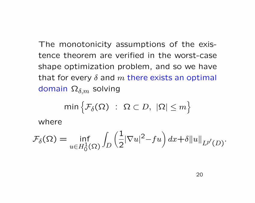
The monotonicity assumptions of the exis-

tence theorem are verified in the worst-case

shape optimization problem, and so we have

that for every δ and m there exists an optimal

domain Ωδ,m solving

minFδ(Ω) : Ω ⊂ D, |Ω| ≤ m

where

Fδ(Ω) = infu∈H1

0(Ω)

∫D

(1

2|∇u|2−fu

)dx+δ‖u‖

Lp′(D)

.

20

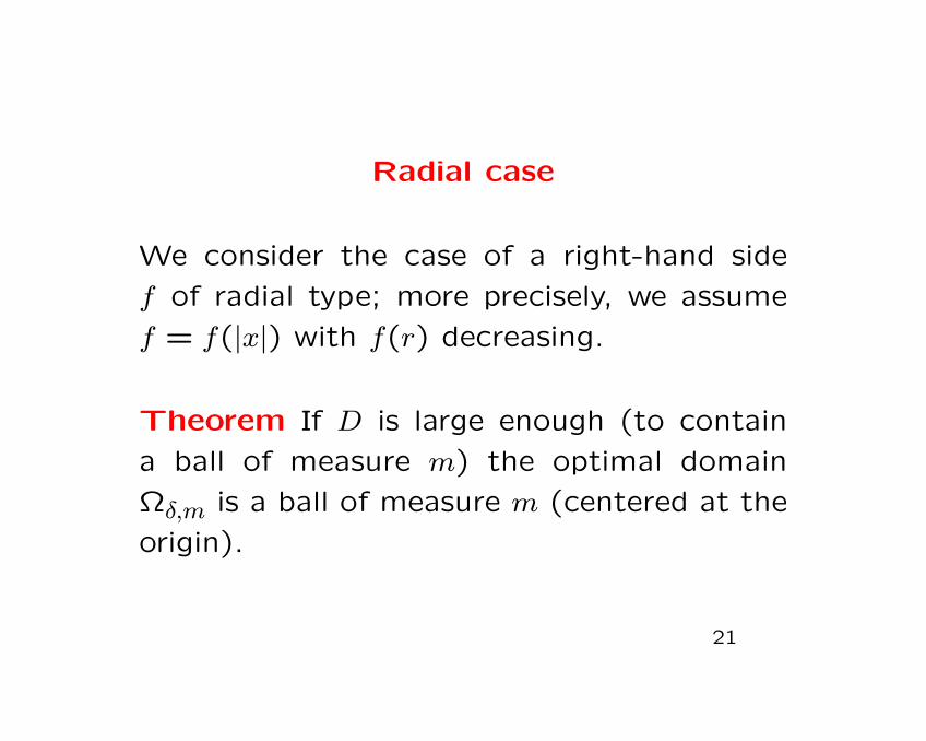
Radial case

We consider the case of a right-hand side

f of radial type; more precisely, we assume

f = f(|x|) with f(r) decreasing.

Theorem If D is large enough (to contain

a ball of measure m) the optimal domain

Ωδ,m is a ball of measure m (centered at the

origin).

21

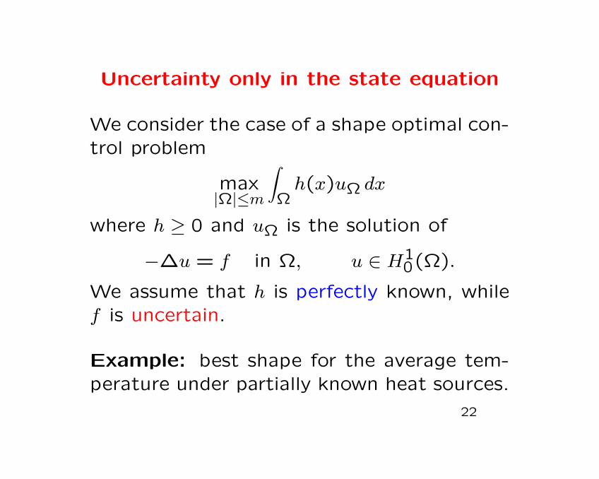
Uncertainty only in the state equation

We consider the case of a shape optimal con-trol problem

max|Ω|≤m

∫Ωh(x)uΩ dx

where h ≥ 0 and uΩ is the solution of

−∆u = f in Ω, u ∈ H10(Ω).

We assume that h is perfectly known, whilef is uncertain.

Example: best shape for the average tem-perature under partially known heat sources.

22

Again, by the fact that the resolvent opera-

tor RΩ is self-adjoint, we can write the worst

case functional as

Fδ(Ω) = sup‖g‖p≤δ

−∫DhR(f + g) dx

= sup‖g‖p≤δ

−∫D

(fR(h) + gR(h)

)dx

=∫D−f(x)wΩ dx+ δ‖wΩ‖Lp′(D)

where

−∆wΩ = h in Ω, wΩ ∈ H10(Ω).

23

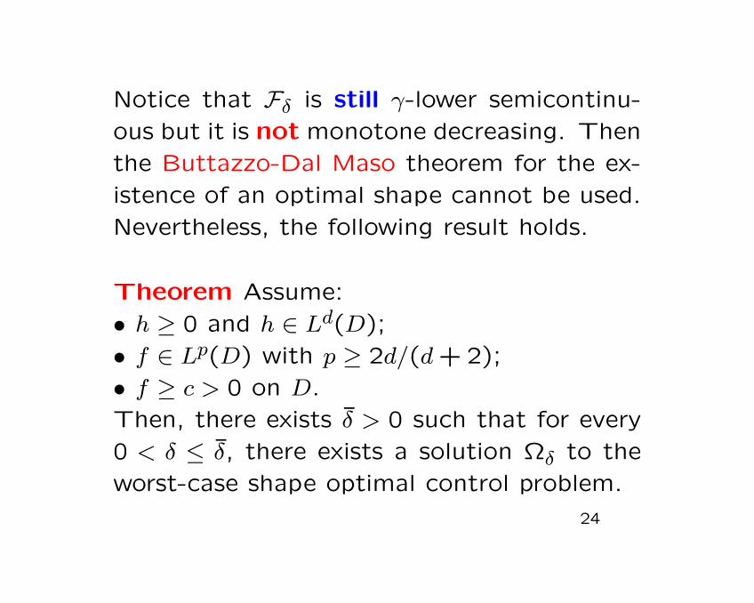
Notice that Fδ is still γ-lower semicontinu-

ous but it is not monotone decreasing. Then

the Buttazzo-Dal Maso theorem for the ex-

istence of an optimal shape cannot be used.

Nevertheless, the following result holds.

Theorem Assume:

• h ≥ 0 and h ∈ Ld(D);

• f ∈ Lp(D) with p ≥ 2d/(d+ 2);

• f ≥ c > 0 on D.

Then, there exists δ > 0 such that for every

0 < δ ≤ δ, there exists a solution Ωδ to the

worst-case shape optimal control problem.

24

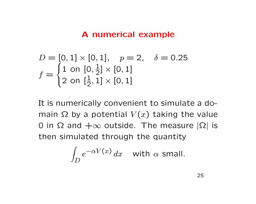
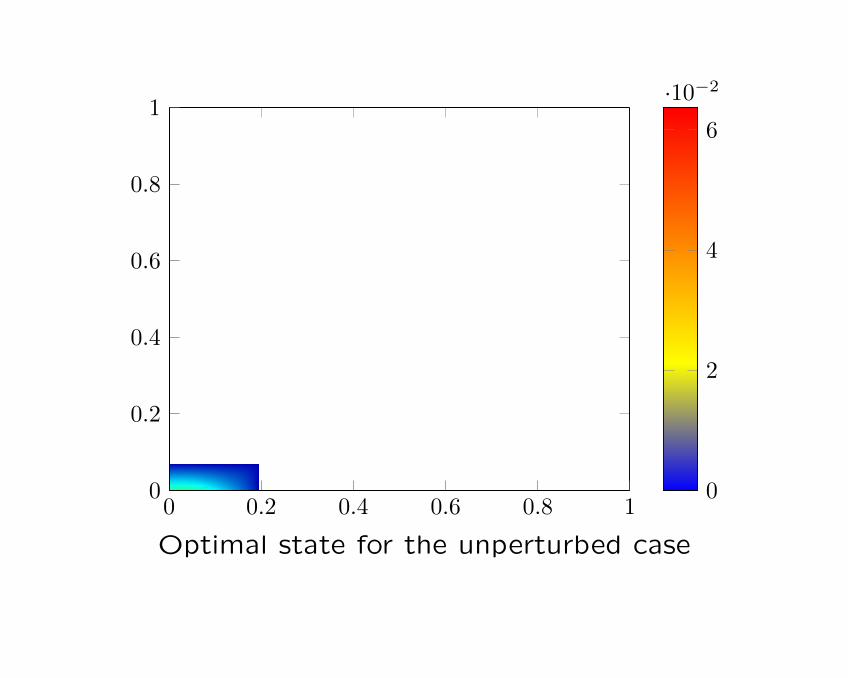
A numerical example

D = [0,1]× [0,1], p = 2, δ = 0.25

f =

1 on [0, 12]× [0,1]

2 on [12,1]× [0,1]

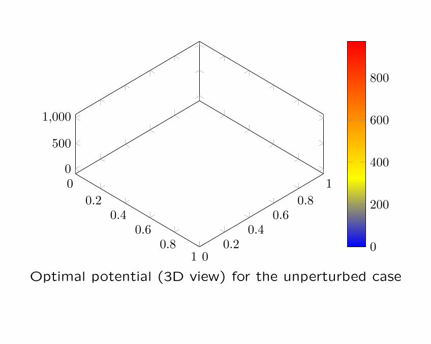
It is numerically convenient to simulate a do-

main Ω by a potential V (x) taking the value

0 in Ω and +∞ outside. The measure |Ω| is

then simulated through the quantity∫De−αV (x) dx with α small.

25

More precisely this approximation has to be

stated in terms on Γ-convergence, proved in

[BGRV, JEP 2014].

The simulation has been made by J.C. Bel-

lido using:

• FreeFEM++

• the Method of Moving Asymptotes (a kind

of gradient method widely used for Topology

and Structural Optimization problems)

• a mesh of 50× 50 elements.

26

0 0.2 0.4 0.6 0.8 10

0.2

0.4

0.6

0.8

1

0

200

400

600

800

Optimal potential for the unperturbed case

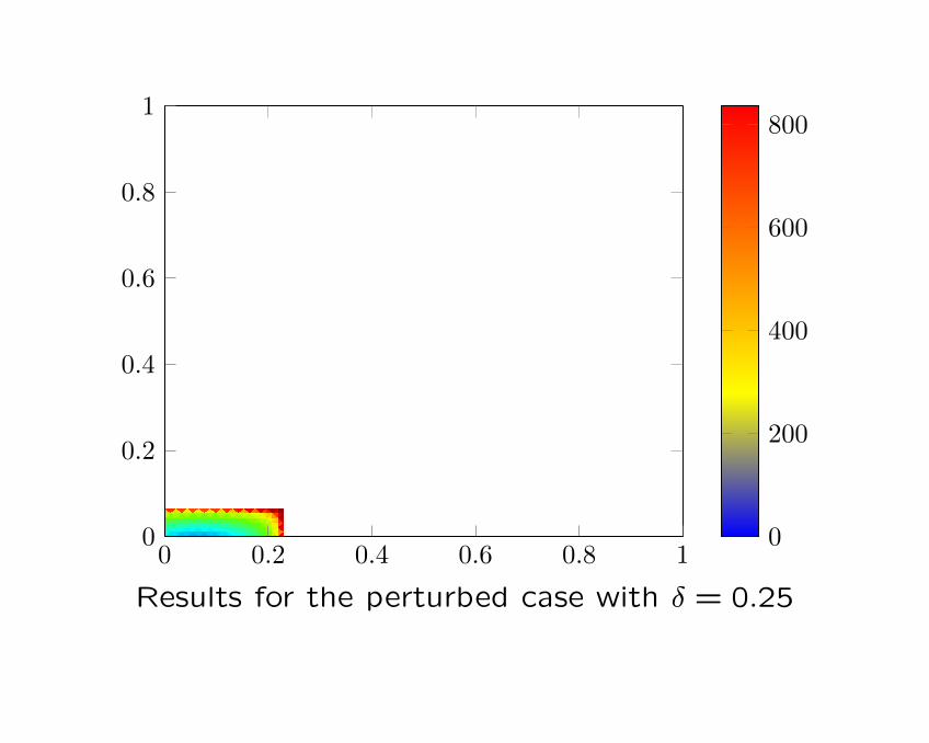
0 0.2 0.4 0.6 0.8 10

0.2

0.4

0.6

0.8

1

0

200

400

600

800

Results for the perturbed case with δ = 0.25

0 0.2 0.4 0.6 0.8 10

0.2

0.4

0.6

0.8

1

0

2

4

6

·10−2

Optimal state for the unperturbed case

0 0.2 0.4 0.6 0.8 10

0.2

0.4

0.6

0.8

1

0

1

2

3

4

·10−2

Optimal state for the perturbed case with δ = 0.25

0

0.20.4

0.60.8

1 00.2

0.40.6

0.8

10

500

1,000

0

200

400

600

800

Optimal potential (3D view) for the unperturbed case

0

0.20.4

0.60.8

1 00.2

0.40.6

0.8

10

500

0

200

400

600

800

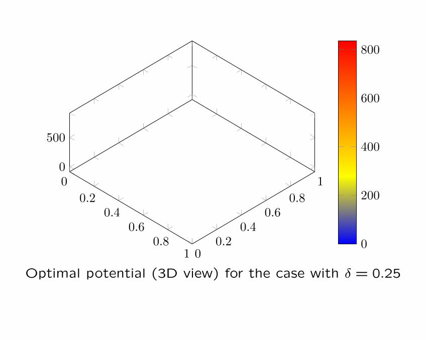
Optimal potential (3D view) for the case with δ = 0.25

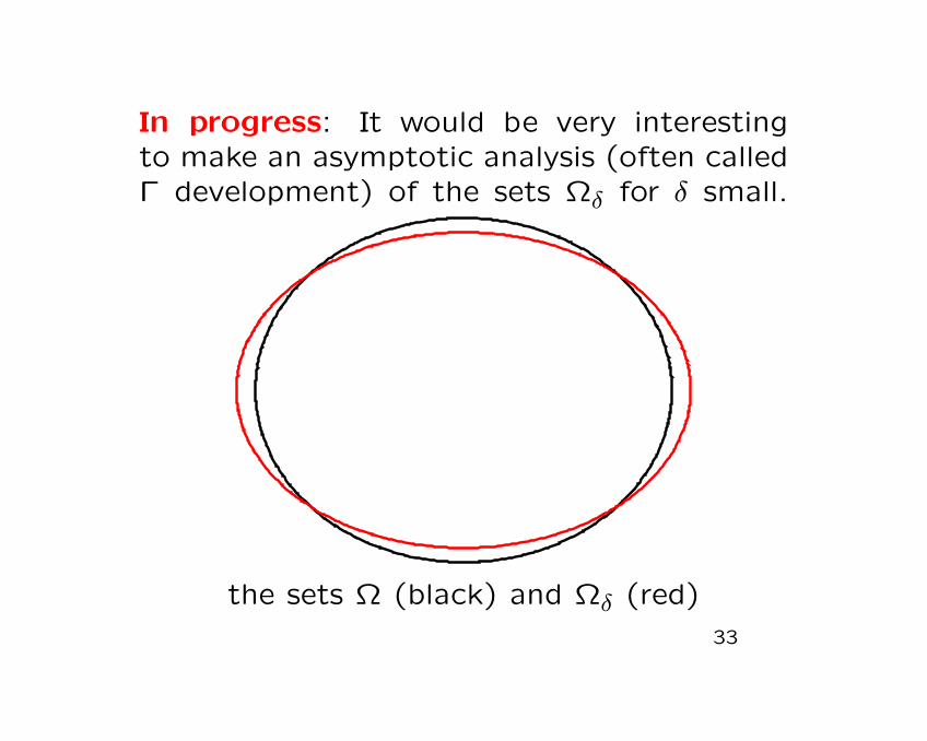
In progress: It would be very interestingto make an asymptotic analysis (often calledΓ development) of the sets Ωδ for δ small.

the sets Ω (black) and Ωδ (red)

33

The expected result is that Ωδ is (asymptot-

ically) equal to Ω with a boundary layer Σδ

of local thickness δh(σ)

Σδ =x = tν(σ), σ ∈ ∂Ω, −δh−(σ) < t < δh+(σ)

for a suitable function h to be characterized,

with∫∂Ω h dσ = 0.

34

Happy birthday Piermarco

and

welcome among seniors...