Embed Size (px)
Citation preview
MATHEMATICAL BIOSCIENCES http://www.mbejournal.org/AND ENGINEERINGVolume 4, Number 3, July 2007 pp. 373–402
STOCHASTIC AND DETERMINISTIC MODELS FORAGRICULTURAL PRODUCTION NETWORKS
P. Bai1, H.T. Banks2, S. Dediu2,3, A.Y. Govan2, M. Last4, A.L. Lloyd2,H.K. Nguyen2,5, M.S. Olufsen2, G. Rempala6, and B.D. Slenning7
1Department of Statistics, University of North Carolina, Chapel Hill, NC
2Center for Research in Scientific Computation and Department of MathematicsNorth Carolina State University, Raleigh, NC
3Statistical and Applied Mathematical Sciences Institute, Research Triangle Park, NC
4National Institute of Statistical Sciences, Research Triangle Park, NC
5 Center for Naval Analyses, Alexandria, VA
6Department of Mathematics and Statistics, University of Louisville, KY
7Department of Population Health and Pathobiology, College of Veterinary MedicineNorth Carolina State University, Raleigh, NC
(Communicated by Hal Smith)
Abstract. An approach to modeling the impact of disturbances in an agricul-tural production network is presented. A stochastic model and its approximatedeterministic model for averages over sample paths of the stochastic systemare developed. Simulations, sensitivity and generalized sensitivity analyses aregiven. Finally, it is shown how diseases may be introduced into the networkand corresponding simulations are discussed.
1. Introduction. The current production methods for livestock follow the just-in-time philosophy of manufacturing industries. Feedstock and animals are grown indifferent areas. Animals are moved from one farm to another, depending on theirage. Unfortunately, shocks propagate rapidly through such systems; an interruptionto the feed supply has a much larger impact when farms have minimal surplussupplies in-stock than when they have large reserves. The just-in-time movementof animals between farms serves as another vulnerability. Stopping movement ofanimals to and from a farm with animals infected by a disease will have effects thatquickly spread through the system. Nurseries supplying the farm will have nowhereto send their animals as they grow up. Finishers and slaughterhouses supplied bythe farm will have their supply interrupted.
The devastating foot-and-mouth disease (FMD) that hit the United Kingdom(UK) in 2001 lead to the slaughter of millions of animals. The outbreak shookmany Western nations as citizens watched a nation with an advanced animal healthsurveillance and response system fail to get FMD under control, in part becausethe UK was unable to mount a rapid response in the face of modern agricultural
2000 Mathematics Subject Classification. 60J20, 34A34, 49Q12, 92D30.
Key words and phrases. agricultural production networks, stochastic and deterministic models,sensitivity and generalized sensitivity functions, foot-and-mouth disease.
373
374BAI, BANKS, DEDIU, GOVAN, LAST, LLOYD, NGUYEN, OLUFSEN, REMPALA, SLENNING
marketing systems [15]. In an effort to eradicate the disease, the marketing chan-nels were stopped, leaving uninfected producers with no income to maintain theirlivestock and no means to move them to locations where feed, shelter, and othersupport were available. As a result, between six million and ten million animalswere destroyed in the UK over seven months, with more than one-third of thoseanimals being destroyed for welfare reasons [41]. Two years after the outbreak, ani-mal agriculture in the UK was still declining, a chilling postscript to the widespreadinfrastructure damage FMD had wrought on the nation [37].
More recently, the world has witnessed the apparent failure of widespread na-tional and international plans for using animal destruction to stem the spread ofthe highly pathogenic H5N1 strain of avian influenza. In a process frighteninglyreminiscent of the UK FMD experience, the programs have also allowed domes-tic markets within and beyond affected countries to suffer. Global consumption ofpoultry has dropped enough to cause US domestic producers (e.g., Tyson, Pilgrim’sPride, et al.) to absorb decreased demand and decreased prices. This drop hastranslated to decreases, as well, in non-poultry markets, exacerbating the marketeffects of a disease not even present in the Western hemisphere [19]. It has be-come painfully apparent that in the large-scale, interdependent, and highly mobileanimal agriculture industry of the USA, the unintended consequences and marketripple effects of a disease incursion into our system could be even more severe thanwhat was witnessed in the UK in 2001 and across Europe in 2005-6, and couldinduce decision-makers to call for even more draconian measures than previouslyseen. What is needed is a new view of how our emergency response programsmight affect modern animal agriculture, a view that allows workers to assess thepotential for other prevention strategies and responses. The view should also al-low analysts to identify bottlenecks in the food and feed supply chain, and to testpotential mitigation tools, procedures, and practices to increase the resilience ofanimal agriculture to catastrophic animal diseases.
This paper presents initial statistical and mathematical modeling ideas to ad-dress the above issues, using the North Carolina swine industry’s potential responseto FMD as an example. We focused our attention on the North Carolina swine in-dustry because it is the second largest swine industry in the United States, andbecause it is local to us. Our goal was to develop a model that could be used toinvestigate how small perturbations to the agricultural supply system would affectits overall performance. A hurricane that throttles inter-farm transportation for ashort period, or a disease outbreak that spreads through distribution channels areexample causes of the perturbations of interest. In the former case, the just-in-timedelivery systems may not provide enough slack to absorb the shock. In the lattercase, strategies that involve destruction of all livestock in an infected branch of thesystem may be overly harsh; a more moderate response may be as effective withoutthe high toll on the infrastructure.
We model a simplified swine production network in North Carolina containingfour levels of production nodes: growers/sows (Node 1), nurseries (Node 2), finish-ers (Node 3), and processing plants/slaughterhouses (Node 4). At grower or sowfarms (Node 1), the new piglets are born and typically weaned three weeks afterbirth. The three-week old piglets are then moved to the nursery farms (Node 2)to mature for another seven weeks. They are then transferred to the finisher farms(Node 3), where they grow to full market size, which takes about twenty weeks.Once they reach market weight, the matured pigs are moved to the processors
MODELS FOR AGRICULTURAL PRODUCTION NETWORKS 375
(slaughterhouses) (Node 4). Pork products then continue through wholesalers toconsumers. There are also several inputs to the system which we will not consider,such as food, typically corn grown in the Midwest. There are several types of breed-ing farms where purebred stock are raised; these are typically crossed to producehybrid strains for pork production.
Our paper is organized as follows. In Section 2, we formulate a nonlinear stochas-tic model for our agricultural network and show how it can be converted to anequivalent (in a sense made precise below) deterministic differential equation model.This deterministic model readily lends itself to simulations and sensitivity analysistechniques. In Section 3 we present numerical simulations of the production model(without perturbations such as infectious disease), and carry out a sensitivity anal-ysis of the model. Simulations of the model in the presence of an infectious diseaseare presented in Section 4. Finally, in Section 5 we give our conclusions and remarksfor future work.
In addition to the development of models for a typical production network per-mitting perturbations, a significant contribution in this paper is the demonstrationof stochastic, mathematical and computational methodology that is available to do-main scientists, statisticians and applied mathematicians working in a concertedteam effort on complex problems of the type exemplified here. The coauthors ofthis paper constituted such a team organized under the auspices and with the sup-port of the Statistical and Applied Mathematical Sciences Institute (SAMSI) as ayear-long working group in its recent research program on National Defense andHomeland Security.
2. Modeling. We consider stochastic models to track an agricultural network. Weare interested in how the parameters used in the model affect the overall capacityof a network and in how one discerns the existence and location of any bottlenecks.With deterministic models, one can answer the first question with a sensitivityanalysis. Thus, after developing a typical stochastic production model, we alsoshow how to obtain its deterministic approximation. We then demonstrate howto superimpose a simple contagious disease model on the production model thatallows simulation of dynamics and spread of FMD through a production chain.
2.1. Basic Model. We consider a simplified swine production network with fouraggregated nodes: sows (Node 1), nurseries (Node 2), finishers (Node 3), andslaughterhouses (Node 4). Our goal is to study the effects of perturbations withinthe network. This can be done by affecting either the nodes or the transitionsbetween nodes directly or indirectly. For instance, a problem with the breedingfarms would result in a reduction of sows available for producing new piglets. Thiswould result in a reduced rate of transition from Node 1 to Node 2, since wecould not grow as many piglets. We could then track the effect of this through ournetwork.
Although unavoidable in actual production processes, we assume in our examplethat there are no net losses in the network (i.e., the total number of pigs in thenetwork remains constant) and that the only deaths occur at the slaughterhouses.Thus we assume that the number of processed pigs per day at the slaughterhousesis equal to the number of newborn piglets per day at the growers. We can modelreduced birth-rates by reducing the rate at which piglets move to the nurseries.This leads us to deal with a closed network. We note that this approximation isrealistic when the network is efficient and operates at or near full capacity (i.e,
376BAI, BANKS, DEDIU, GOVAN, LAST, LLOYD, NGUYEN, OLUFSEN, REMPALA, SLENNING
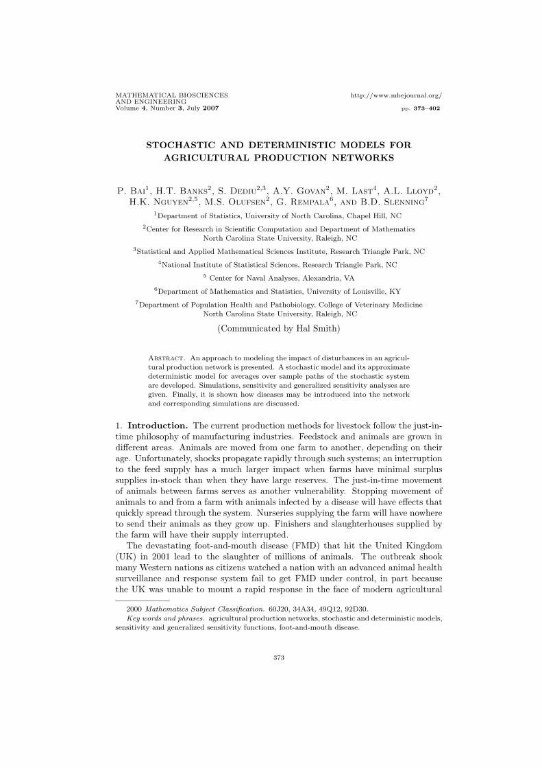
when the number of animals removed from the chain are immediately replaced bynew production/growth, avoiding significant idle times). Our closed network modelfor the swine production is summarized schematically in Figure 1.
SlaughterFinisherNurserySows
N4N3N1 N2
Figure 1. Aggregated agricultural network model.
Each node with corresponding population number Ni, i = 1, . . . , 4, in Figure 1represents an aggregation of all the production units corresponding to that level inthe production network. Given a specific production network, any of the four levelsof the chain may be broken into its constituent units (e.g., farms), and analyzed indetail as a separate subnetwork. The directed edges between the nodes representthe movement of the pigs through the network. The rate is determined by the pigs’residence time, the number of pigs at each node, and the capacity constraints at thecorresponding nodes. Let Li denote the capacity constraint at node i, i = 1, . . . , 4.Since we have a closed network, it is assumed that there is no capacity constraintat Node 1, and therefore we take L1 = ∞. We also define Sm to be the maximumexit rate at Node 4; i.e., the maximum killing capacity at the slaughter house.The residence times at each node, together with the capacity constraints and theslaughterhouse killing capacity, based on very rough estimates of swine productionin North Carolina [1], are given in Table 1.
Table 1. Network parameters based on swine production in NC.
Name Sows Nursery Finisher SlaughterNode N1 N2 N3 N4Piglet residencetime (days) 21(N1→N2) 49(N2→N3) 140(N3→N4) 1(N4→N1)
Assumed capacity(in thousands) ∞ 825 2300 20
2.2. Stochastic and Deterministic Models. We model the evolution of thefood production network shown in Figure 1 as a continuous time discrete statedensity dependent jump Markov Chain (MC) [3, 21] with a discrete state spaceembedded in an R4 non-negative integer lattice L. The state of this MC at time tis denoted by X(t) = (X1(t), . . . , X4(t)), where Xi(t) is the number of pigs at nodei at time t, i = 1, . . . , 4.
The rates of transition of X(t) are nonlinear functions λi : L → [0,∞) fori = 1, . . . , 4, and for x ∈ L are given by:
λ1(x) := q1(x1 − 1, x2 + 1, x3, x4) = k1 x1 (L2 − x2)+λ2(x) := q2(x1, x2 − 1, x3 + 1, x4) = k2 x2 (L3 − x3)+λ3(x) := q3(x1, x2, x3 − 1, x4 + 1) = k3 x3 (L4 − x4)+λ4(x) := q4(x1 + 1, x2, x3, x4 − 1) = k4 min(x4, Sm) (1)
MODELS FOR AGRICULTURAL PRODUCTION NETWORKS 377
where ki, i = 1, . . . , 4, is proportional to the service rate at node i; Li, i = 2, 3, 4,is the buffer size (capacity constraint) at node i and Sm is the slaughter capacityat node 4 as discussed above. For any real z, the symbol (z)+ is defined as thenon-negative part of z, i.e., (z)+ = max(z, 0). Then q1(x1 − 1, x2 + 1, x3, x4) isgiven by
q1(x1 − 1,x2 + 1, x3, x4) ≡
limh→0+
Pr[X(t + h) = (x1 − 1, x2 + 1, x3, x4)|X(t) = (x1, x2, x3, x4)]h
.
The other qi are given similarly.The simple model (1) is formulated under the following assumptions and hy-
potheses. First it is assumed that the transportation rates qi, i = 1, 2, 3, are pro-portional to xi (Li+1− xi+1)+, the product of the number of animals available andthe available capacity at the next node. If no capacity is available, the rate istaken as zero. The rate at the slaughter house (Node 4) is the maximum Sm if asufficient number of animals is available; otherwise all animals present at the nodeare slaughtered on that day. Finally, it is assumed that the network is at or nearsteady-state and maximum efficiency in that the slaughter rate at Node 4 is thesame as the input at Node 1 (this is represented schematically in Figure 1 by thearrow from Node 4 to Node 1). This results in the rate dynamics (9) below withthe output rate at Node 4 the same as the input rate at Node 1.
We remark that the product nonlinearities xi (Li+1−xi+1)+ of (1) where trans-portation occurs more rapidly the further the node level is from capacity (i.e.,the system reacts more rapidly to larger perturbations from capacity) are onlyone possible form for these terms. One could also reasonably argue for alterna-tive terms of the form xi χi+1 where χi+1 is the characteristic function for the set{(Li+1 − xi+1) > 0}, so that the transportation rate from a node depends only onthe number available at that node so long as capacity at the next node has notbeen reached. We remark that in this case the sensitivity analyses below are moredifficult because of a lack of continuity of the dynamics in the system equations.
Let Ri(t) i = 1, . . . , 4, denote the number of times that the ith transition oc-curs by time t. Then Ri is a counting process with intensity λi(X(t)), and thecorresponding stochastic process can be defined by
Ri(t) = Yi
( ∫ t
0
λi(X(s))ds), i = 1 . . . , 4, (2)
where the Yi are independent unit Poisson processes. That is, sample paths ri(t)of Ri(t) are given in terms of sample paths x(t) of X(t) by
ri(t) = Yi
( ∫ t
0
λi(x(s))ds), i = 1 . . . , 4. (3)
We write Ri in this form to illustrate that λi is a rate of the corresponding countingprocess.
Let ei, i = 1, . . . , 4, be standard basis vectors of R4 and define, for i incrementedby one modulo 4, the vectors
νi = e(i+1)(mod4) − ei i = 1, 2, . . . , 4,
378BAI, BANKS, DEDIU, GOVAN, LAST, LLOYD, NGUYEN, OLUFSEN, REMPALA, SLENNING
which represent the vector of changes in system counts at ith transition. We writethe state of the system at time t as
X(t) = X(0) +∑
i
Ri(t)νi = X(0) + νR(t), (4)
where ν is the matrix with rows given by the νi, and R(t) is the (column) vectorwith components Ri(t). In the chemical literature, the matrix νT is often referredto as the stoichiometric matrix [29]. More specifically, we have
X1(t) = X1(0)−R1(t) + R4(t)X2(t) = X2(0) + R1(t)−R2(t)X3(t) = X3(0) + R2(t)−R3(t)X4(t) = X4(0) + R3(t)−R4(t). (5)
The above system typically cannot be solved for a stationary distribution, andan empirical approach based on the so-called Gillespie algorithm [29] can be used toinvestigate the long-term behavior of the system (see Section 3.2). The approximatelarge-population behavior of an appropriately scaled system may be also analyzedwith macroscopic deterministic rate equations, as we shall explain next (the originaltheory is due to Kurtz and is discussed in [21] and the references therein).
Let N be the total network or population size. If N is known we may considerthe animal units per system size or the units concentration in the stochastic processCN (t) = X(t)/N with sample paths cN (t). For large systems, this approach leadsto a deterministic approximation (obtained as solutions to the system rate equationdefined below) to the stochastic equation (4), in terms of c(t), the large sample sizeaverage over sample paths or trajectories cN (t) of CN (t).
We rescale the rate constants ki, Li and Sm as follows:
κ4 = k4, κi = Nki, i = 1, 2 or 3,
sm = Sm/N, li = Li/N. (6)
According to Equation (1), this rescaling implies that
λi(x) = κi xi(Li+1 − xi)+/N = Nκi cNi (li+1 − cN
i )+ i = 1, 2, 3,
andλ4(x) = κ4 min(x4, Sm) = Nκ4 min(cN
4 , sm).
Recall that for large N the Strong Law of Large Numbers (SLLN) for the PoissonProcess Y implies Y (Nu)/N ≈ u [30]. One can use this fact, along with therescaling of the constants as given above, to argue that sample paths ri(t) for thecounting process (2) defined in terms of the sample paths x(t) or cN (t) = x(t)/Nmay be approximated for large N in terms of the deterministic variables c(t), theaverages over sample paths or trajectories cN (t) of CN (t), by
r(N)i (t) =
1N
ri(t) =1N
Yi
( ∫ t
0
λi(x(s))ds)
=1N
Yi
(N
∫ t
0
κicNi (s)(li+1 − cN
i+1(s))+ ds)
≈∫ t
0
κi ci(s)(li+1 − ci+1(s))+ ds for i = 1, 2, 3, (7)
MODELS FOR AGRICULTURAL PRODUCTION NETWORKS 379
and similarly
r(N)4 (t) =
1N
r4(t) ≈∫ t
0
κ4 min(c4(s), sm) ds.
For a full and rigorous discussion of this “approximation in mean,” see Chapters6.4 and 11 of [21] and Chapter 5 of [3]. The averages c(t) satisfy a system ofdeterministic ordinary differential equations which can be heuristically derived bybeginning with Equation (5). Upon dividing both sides of each equation by Nand applying the above, we obtain the rate equations, (i.e., the system of integralequations approximating via the SLLN the original stochastic system), as follows:
cN1 (t) = c1(0)− r
(N)1 (t) + r
(N)4 (t)
≈ c1(0)−∫ t
0
κ1c1(s)(l2 − c2(s))+ ds +∫ t
0
κ4 min(c4(s), sm) ds
cN2 (t) = c2(0) + r
(N)1 (t)− r
(N)2 (t)
≈ c2(0)−∫ t
0
κ2c2(s)(l3 − c3(s))+ ds +∫ t
0
κ1c1(s)(l2 − c2(s))+ ds
cN3 (t) = c3(0) + r
(N)2 (t)− r
(N)3 (t)
≈ c3(0)−∫ t
0
κ3c3(s)(l4 − c4(s))+ ds +∫ t
0
κ2c2(s)(l3 − c3(s))+ ds
cN4 (t) = c4(0) + r
(N)3 (t)− r
(N)4 (t)
≈ c4(0) +∫ t
0
κ3c3(s)(l4 − c4(s))+ ds−∫ t
0
κ4 min(c4(s), sm) ds. (8)
Upon approximating the cNi (t) on the left above by the ci(t) and differentiating
the resulting equations, we find that the integral equation system is equivalent toa system of ordinary differential equations for c(t) ∈ R4 given by
dc1(t)dt
= −κ1c1(t)(l2 − c2(t))+ + κ4min(c4(t), sm)
dc2(t)dt
= −κ2c2(t)(l3 − c3(t))+ + κ1c1(t)(l2 − c2(t))+
dc3(t)dt
= −κ3c3(t)(l4 − c4(t))+ + κ2c2(t)(l3 − c3(t))+
dc4(t)dt
= −κ4min(c4(t), sm) + κ3c3(t)(l4 − c4(t))+ (9)
with the initial conditions c(0) = c0. As we shall see in the next section, solutionsof these equations yield quite good approximations to the sample paths of thestochastic system.
3. Computations and Model Comparison.
3.1. Model Parameter Values. To carry out numerical simulations and to com-pare the results of the stochastic and deterministic models (equations (5) and (9),respectively), we must choose reasonable values for all model parameters. We notethat our paper focuses on methodological issues and, for confidentiality and pro-prietary reasons, only limited information on the swine production network was
380BAI, BANKS, DEDIU, GOVAN, LAST, LLOYD, NGUYEN, OLUFSEN, REMPALA, SLENNING
available to us. Thus some of these parameter values may be only rough approxi-mations of those that might be obtained using inverse problem techniques with datafrom actual production networks [1]. Consequently, the subsequent discussions inthis paper are in no way an attempt to validate the above models. Nonetheless,we believe that the order-of-magnitude approximate parameter values we are usinghere are sufficient to allow us to develop and demonstrate effective use of methodsand techniques which could be used with actual production network based param-eters.
The parameters of the stochastic model, with the exception of the transition rateconstants ki, are given in Table 1. From the expressions for the transition rates(1), we see that the residence times, ti, that pigs spend at node i are given by
ti =1ki
1(Li+1 −Xi+1(t))
for i = 1, 2 or 3, (10)
and t4 = 1/k4 = 1. As discussed above, the nonlinear form of the transition rates(1) means that the residence time at a given node depends on how far the followingnode is below its capacity. Consequently, we determine the ki by assuming that thegiven residence times pertain to the network in its equilibrium state.
Considering the deterministic model equations (9), we see that, if there is tobe a flow through the system, the equilibrium population sizes N∗
i = Nc∗i at eachnode must be less than the capacities of the nodes. It is then straightforward tosee that the equilibrium numbers of individuals at each of the first three nodes areproportional to the ti. This makes intuitive sense, since no loss occurs as individualsmove between nodes, and so, at equilibrium, the relative residence times must equalthe relative numbers of individuals at the nodes. This argument need not applyto the slaughter node, however, since individuals will spend longer there than thespecified one-day residence time if the equilibrium value N∗
4 is greater than Sm.The flow rate from node four back to node one is the smaller of N∗
4 and Sm, andso we have that
(N∗1 , N∗
2 , N∗3 , N∗
4 ) ={
(t1N∗4 , t2N
∗4 , t3N
∗4 , N∗
4 ) if N∗4 ≤ Sm
(t1Sm, t2Sm, t3Sm, N∗4 ) otherwise. (11)
Notice that solving for the equilibrium of the deterministic model does not give usthe value of N∗
4 : since the network is closed, the total size of the population is equalto its value at the initial time. The values of the ki, for i = 1, 2 and 3, are thengiven by
ki =1
ti(Li+1 −N∗
i+1
) . (12)
The parameter values and the initial states for the system (5) are tabulated in Table2.
To obtain the parameters we use in our deterministic simulations we simplyrescale the parameters in Table 2 by the total network size N = X1(t0) + X2(t0) +X3(t0) + X4(t0) = 3, 165, 000, using equation (6) and ci(t0) = Xi(t0)/N for i =1, . . . , 4. The results are given below in Table 3.
MODELS FOR AGRICULTURAL PRODUCTION NETWORKS 381
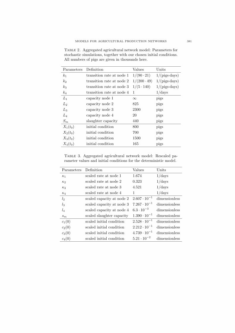
Table 2. Aggregated agricultural network model: Parameters forstochastic simulations, together with our chosen initial conditions.All numbers of pigs are given in thousands here.
Parameters Definition Values Unitsk1 transition rate at node 1 1/(90 · 21) 1/(pigs·days)k2 transition rate at node 2 1/(200 · 49) 1/(pigs·days)k3 transition rate at node 3 1/(5 · 140) 1/(pigs·days)k4 transition rate at node 4 1 1/daysL1 capacity node 1 ∞ pigsL2 capacity node 2 825 pigsL3 capacity node 3 2300 pigsL4 capacity node 4 20 pigsSm slaughter capacity 440 pigsX1(t0) initial condition 800 pigsX2(t0) initial condition 700 pigsX3(t0) initial condition 1500 pigsX4(t0) initial condition 165 pigs
Table 3. Aggregated agricultural network model: Rescaled pa-rameter values and initial conditions for the deterministic model.
Parameters Definition Values Unitsκ1 scaled rate at node 1 1.674 1/daysκ2 scaled rate at node 2 0.323 1/daysκ3 scaled rate at node 3 4.521 1/daysκ4 scaled rate at node 4 1 1/daysl2 scaled capacity at node 2 2.607 · 10−1 dimensionlessl3 scaled capacity at node 3 7.267 · 10−1 dimensionlessl4 scaled capacity at node 4 6.3 · 10−3 dimensionlesssm scaled slaughter capacity 1.390 · 10−1 dimensionlessc1(0) scaled initial condition 2.528 · 10−1 dimensionlessc2(0) scaled initial condition 2.212 · 10−1 dimensionlessc3(0) scaled initial condition 4.739 · 10−1 dimensionlessc4(0) scaled initial condition 5.21 · 10−2 dimensionless
382BAI, BANKS, DEDIU, GOVAN, LAST, LLOYD, NGUYEN, OLUFSEN, REMPALA, SLENNING
3.2. Stochastic Simulations. The standard method for the stochastic simulationof the discrete state continuous time Markov Chain of the type considered here isbased on a standard Monte Carlo algorithm, also known as the Gillespie algorithm[29]. This algorithm is described below:
1. For a given state of the system x, compute λi(x) for i = 1 . . . , M (in our caseM = 4).
2. Calculate the summation of the rates λ =M∑
i=1
λi(x) and simulate the time
until the next transition by drawing from an exponential distribution withmean 1/λ.
3. Simulate the transition type RX ∈ {1, . . . , 4} by drawing from the discretedistribution with P (RX = i) = λi(x)/λ.
4. Update the system state x and repeat.
Using the above algorithm implemented in the statistical software R [40], wecarried out numerous simulations for the model (5) with the initial conditions andvalues for parameters q∗ = (k1 . . . , k4, Sm, L2, L3, L4) given in Table 2.
0 20 40 60 80 1000
500
1000
1500
2000
2500
time (days)
Num
ber
of p
igs
(in th
ousa
nds)
Stochastic Simulations
Realiz1Realiz2Realiz3Realiz4Realiz5
X3
X1
X2
X4
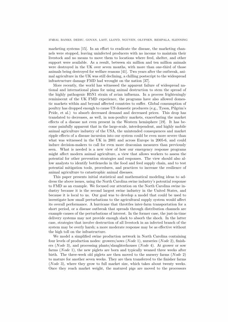
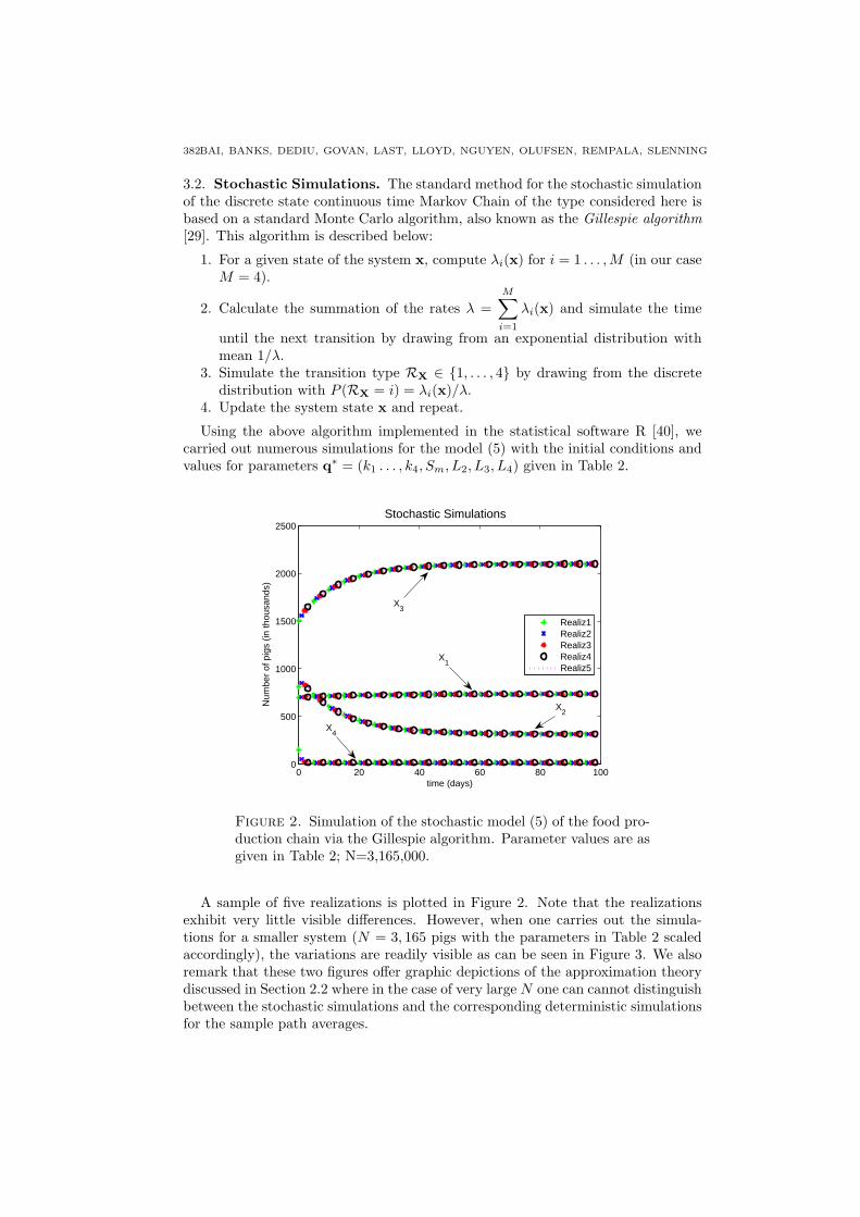
Figure 2. Simulation of the stochastic model (5) of the food pro-duction chain via the Gillespie algorithm. Parameter values are asgiven in Table 2; N=3,165,000.
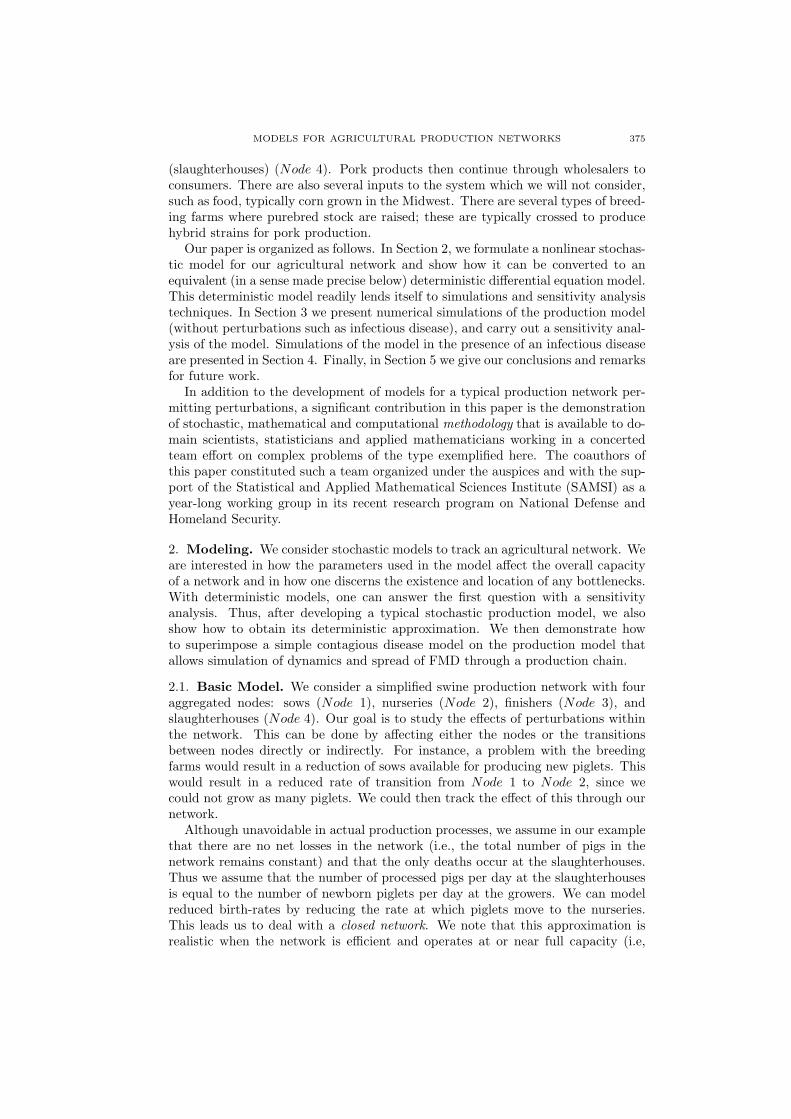
A sample of five realizations is plotted in Figure 2. Note that the realizationsexhibit very little visible differences. However, when one carries out the simula-tions for a smaller system (N = 3, 165 pigs with the parameters in Table 2 scaledaccordingly), the variations are readily visible as can be seen in Figure 3. We alsoremark that these two figures offer graphic depictions of the approximation theorydiscussed in Section 2.2 where in the case of very large N one can cannot distinguishbetween the stochastic simulations and the corresponding deterministic simulationsfor the sample path averages.
MODELS FOR AGRICULTURAL PRODUCTION NETWORKS 383
0 20 40 60 80 1000
500
1000
1500
2000
2500
time (days)
Num
ber
of p
igs
Stochastic Simulations
Realiz1Realiz2Realiz3Realiz4Realiz5
X4
X3
X1
X2
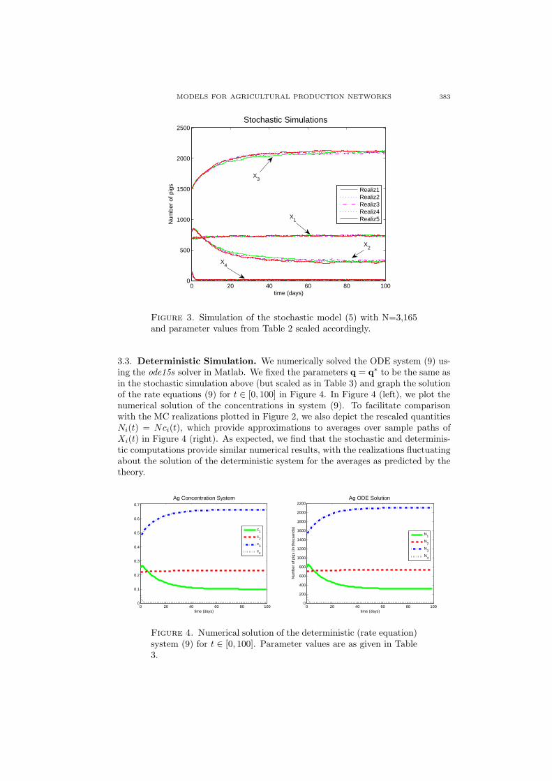
Figure 3. Simulation of the stochastic model (5) with N=3,165and parameter values from Table 2 scaled accordingly.
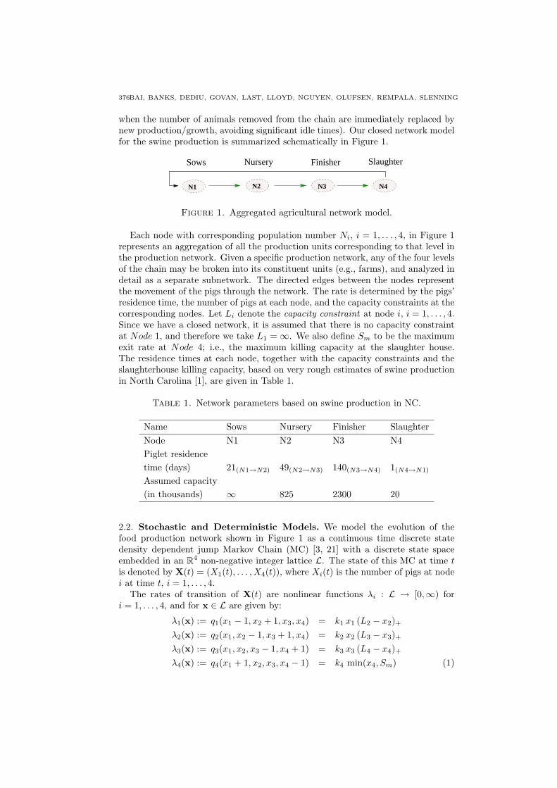
3.3. Deterministic Simulation. We numerically solved the ODE system (9) us-ing the ode15s solver in Matlab. We fixed the parameters q = q∗ to be the same asin the stochastic simulation above (but scaled as in Table 3) and graph the solutionof the rate equations (9) for t ∈ [0, 100] in Figure 4. In Figure 4 (left), we plot thenumerical solution of the concentrations in system (9). To facilitate comparisonwith the MC realizations plotted in Figure 2, we also depict the rescaled quantitiesNi(t) = Nci(t), which provide approximations to averages over sample paths ofXi(t) in Figure 4 (right). As expected, we find that the stochastic and determinis-tic computations provide similar numerical results, with the realizations fluctuatingabout the solution of the deterministic system for the averages as predicted by thetheory.
0 20 40 60 80 1000
0.1
0.2
0.3
0.4
0.5
0.6
0.7
time (days)
Ag Concentration System
c1
c2
c3
c4
0 20 40 60 80 1000
200
400
600
800
1000
1200
1400
1600
1800
2000
2200
time (days)
Num
ber
of p
igs
(in th
ousa
nds)
Ag ODE Solution
N1
N2
N3
N4
Figure 4. Numerical solution of the deterministic (rate equation)system (9) for t ∈ [0, 100]. Parameter values are as given in Table3.
384BAI, BANKS, DEDIU, GOVAN, LAST, LLOYD, NGUYEN, OLUFSEN, REMPALA, SLENNING
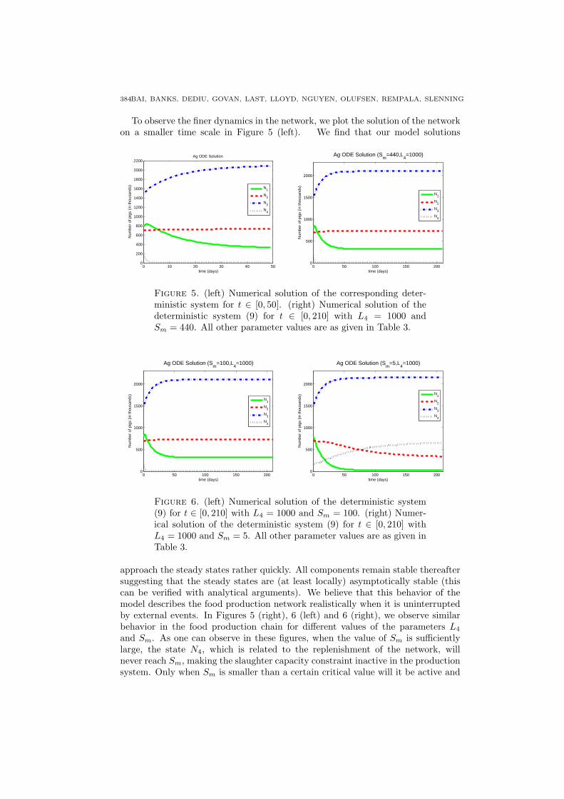
To observe the finer dynamics in the network, we plot the solution of the networkon a smaller time scale in Figure 5 (left). We find that our model solutions
0 10 20 30 40 500
200
400
600
800
1000
1200
1400
1600
1800
2000
2200
time (days)
Num
ber
of p
igs
(in th
ousa
nds)
Ag ODE Solution
N1
N2
N3
N4
0 50 100 150 2000
500
1000
1500
2000
time (days)
Num
ber
of p
igs
(in th
ousa
nds)
Ag ODE Solution (Sm
=440,L4=1000)
N1
N2
N3
N4
Figure 5. (left) Numerical solution of the corresponding deter-ministic system for t ∈ [0, 50]. (right) Numerical solution of thedeterministic system (9) for t ∈ [0, 210] with L4 = 1000 andSm = 440. All other parameter values are as given in Table 3.
0 50 100 150 2000
500
1000
1500
2000
time (days)
Num
ber
of p
igs
(in th
ousa
nds)
Ag ODE Solution (Sm
=100,L4=1000)
N1
N2
N3
N4
0 50 100 150 2000
500
1000
1500
2000
time (days)
Num
ber
of p
igs
(in th
ousa
nds)
Ag ODE Solution (Sm
=5,L4=1000)
N1
N2
N3
N4
Figure 6. (left) Numerical solution of the deterministic system(9) for t ∈ [0, 210] with L4 = 1000 and Sm = 100. (right) Numer-ical solution of the deterministic system (9) for t ∈ [0, 210] withL4 = 1000 and Sm = 5. All other parameter values are as given inTable 3.
approach the steady states rather quickly. All components remain stable thereaftersuggesting that the steady states are (at least locally) asymptotically stable (thiscan be verified with analytical arguments). We believe that this behavior of themodel describes the food production network realistically when it is uninterruptedby external events. In Figures 5 (right), 6 (left) and 6 (right), we observe similarbehavior in the food production chain for different values of the parameters L4
and Sm. As one can observe in these figures, when the value of Sm is sufficientlylarge, the state N4, which is related to the replenishment of the network, willnever reach Sm, making the slaughter capacity constraint inactive in the productionsystem. Only when Sm is smaller than a certain critical value will it be active and
MODELS FOR AGRICULTURAL PRODUCTION NETWORKS 385
in this case we observe accumulation of animals in the slaughter house (e.g., seeFigure 6 (right)). These calculations along with numerous others we carried outsuggest reasonable stability properties of the production chain in the absence ofany interventions such as FMD (we will investigate such disturbances below).
3.4. Sensitivity Analysis. In this section, we perform a sensitivity analysis of thedeterministic model (9), investigating how much the solution of the system changeswhen the rates κi, the capacities li, or the initial conditions c0i, i = 1, . . . , 4 change.This analysis will be used to identify the parameters and the initial conditions towhich the system is the most and least sensitive.
A second issue we address here, which is of great interest for inverse or parameterestimation problems in a typical nonlinear regression model, is the sensitivity of theparameter estimates with respect to the data measurements. We carry out this anal-ysis by means of the generalized sensitivity functions (GSF) recently introduced byThomaseth and Cobelli [44]; these are specifically designed for input-output identi-fication experiments. GSF are based on information theoretical criteria (the Fisherinformation matrix) and, when used in conjunction with the traditional sensitivityfunctions, give a more accurate picture of the time distribution of the informationcontent of measured outputs with respect to individual model parameters.
To use the well developed sensitivity analysis for the theory of dynamical systemsfor our purposes, we begin by writing the system (9) in vector form. We introducethe notation c(t) = (c1(t), c2(t), c3(t), c4(t))T ,q = (κ1, ..., κ4, sm, l2, ..., l4), c0 =(c1(0), ..., c4(0))T , and denote by F = (f1, f2, f3, f4)T the vector function whoseentries are given by the expressions in the right side of (9). Then F : R4×R8 → R4,and we can write our ODE system in the general vector form
dcdt
(t) = F(c,q), (13)
c(0) = c0.
To quantify the variation in the state variable c(t) with respect to changes in theparameters qj , j = 1, . . . , 8 and the initial conditions c0k, k = 1, . . . , 4, we arenaturally led to consider the sensitivity matrices
Y = {yij}i=1,...,4j=1,...,8
={
∂ci
∂qj
}i=1,...,4j=1,...,8
, (14)
and
Z = {zik}i=1,...,4k=1,...,4
={
∂ci
∂c0k
}i=1,...,4k=1,...,4
. (15)
We note that since our function F is sufficiently regular, the solutions ci are differ-entiable with respect to qj and c0k, and therefore our sensitivity matrices Y and Zare well defined. The physical interpretation of the sensitivity matrices is obvious.Similar to the partial derivatives through which they are defined, they have a localcharacter (in time and parameters). If, for example, the entry yij = ∂ci/∂qj ofthe matrix Y takes values very close to zero in a certain time subinterval, then thestate variable ci is insensitive to the parameter qj on that particular subinterval.The same entry yij can take large values on a different subinterval, indicating thatin this time subinterval, the state variable ci is very sensitive to the parameter qj .
386BAI, BANKS, DEDIU, GOVAN, LAST, LLOYD, NGUYEN, OLUFSEN, REMPALA, SLENNING
From sensitivity analysis theory for dynamical systems [10, 20, 25, 36, 42], wealso know that Y(t) is a 4× 8 matrix that satisfies the ODE system
Y(t) = Fc(c,q)Y(t) + Fq(c,q), (16)Y(0) = 04×8,
and Z(t) is a 4× 4 matrix that satisfies
Z(t) = Fc(c,q)Z(t), (17)Z(0) = I4×4.
Here we have used the notation Fc = ∂F/∂c and Fq = ∂F/∂q for the 4×4 and the4×8 Jacobian matrices of F with respect to c and q, respectively, while 0 and I arethe zero and the identity matrices with appropriate dimensions. Note that whileequations (16), (17) are linear in Y and Z, they must be solved in tandem withequation (13), which is nonlinear. Consequently, the sensitivity analysis involvesthe solution of a set of nonlinear equations.
We will compute the sensitivity of the system (13) with respect to q and c0
when the solutions are essentially at steady state. We carry this out by numericallysolving the systems (16) and (17) for the same values of the parameters q = q∗ andinitial conditions c = c∗0 as used in the stochastic simulations presented above (i.e.,those given in Table 3) and by evaluating the solution at the fixed time t = 210(arbitrarily chosen, but sufficiently large for our system to closely approach itssteady state). Due to the nature of our problem, in which the parameters havedifferent units and the state variables vary widely over many orders of magnitude,it is appropriate to consider the relative sensitivities Sci,qj defined as the limit ofthe relative change in ci divided by the relative change in qj when the relativechange in qj goes to zero; i.e.,
Sci,qj = lim∆qj→0
∆ci/ci
∆qj/qj. (18)
A simple analysis of the definition above (assuming that both ci and qj are nonzero)yields that the relative sensitivity Sci,qj can be obtained by normalizing the usualsensitivities ∂ci/∂qj such that
Sci,qj =∂ci
∂qj· qj
ci. (19)
We note that the Sci,qj are dimensionless variables, invariant with respect to changesin units for ci and qj , which we can utilize to compare the degree of sensitivity ofthe state variables with respect to different parameters. In Table 4, we tabulatethe relative sensitivities at time t = 210 of each state variable ci with respect toeach parameter qj and each initial condition c0k. For any fixed parameter/initialcondition, we also tabulate the sensitivity of the system, cumulatively defined as theEuclidean norm of the relative sensitivities of the four state variables with respectto that parameter/initial condition. In other words, the sensitivity of the systemwith respect to qj is given by
Sqj =[ 4∑
i=1
S2ci,qj
]1/2
. (20)
For the particular choice of the parameters q = q∗ and for the particular initialcondition c0 = c∗0, the data displayed in the last column of Table 4 reveal that near
MODELS FOR AGRICULTURAL PRODUCTION NETWORKS 387
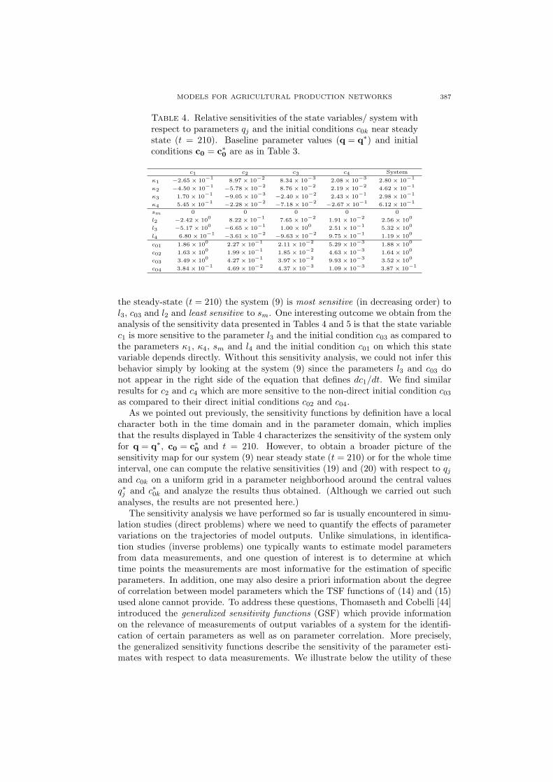
Table 4. Relative sensitivities of the state variables/ system withrespect to parameters qj and the initial conditions c0k near steadystate (t = 210). Baseline parameter values (q = q∗) and initialconditions c0 = c∗0 are as in Table 3.
c1 c2 c3 c4 System
κ1 −2.65× 10⁻¹
8.97× 10⁻²
8.34× 10⁻³
2.08× 10⁻³
2.80× 10⁻¹
κ2 −4.50× 10⁻¹ −5.78× 10
−28.76× 10
−22.19× 10
−24.62× 10
−1
κ3 1.70× 10⁻¹ −9.05× 10
−3 −2.40× 10⁻²
2.43× 10⁻¹
2.98× 10⁻¹
κ4 5.45× 10⁻¹ −2.28× 10
−2 −7.18× 10⁻² −2.67× 10
−16.12× 10
−1
sm 0 0 0 0 0
l2 −2.42× 100
8.22× 10⁻¹
7.65× 10⁻²
1.91× 10⁻²
2.56× 100
l3 −5.17× 100 −6.65× 10
−11.00× 10
02.51× 10
−15.32× 10
0
l4 6.80× 10⁻¹ −3.61× 10
−2 −9.63× 10⁻²
9.75× 10⁻¹
1.19× 100
c01 1.86× 100
2.27× 10⁻¹
2.11× 10⁻²
5.29× 10⁻³
1.88× 100
c02 1.63× 100
1.99× 10⁻¹
1.85× 10⁻²
4.63× 10⁻³
1.64× 100
c03 3.49× 100
4.27× 10⁻¹
3.97× 10⁻²
9.93× 10⁻³
3.52× 100
c04 3.84× 10⁻¹
4.69× 10⁻²
4.37× 10⁻³
1.09× 10⁻³
3.87× 10⁻¹
the steady-state (t = 210) the system (9) is most sensitive (in decreasing order) tol3, c03 and l2 and least sensitive to sm. One interesting outcome we obtain from theanalysis of the sensitivity data presented in Tables 4 and 5 is that the state variablec1 is more sensitive to the parameter l3 and the initial condition c03 as compared tothe parameters κ1, κ4, sm and l4 and the initial condition c01 on which this statevariable depends directly. Without this sensitivity analysis, we could not infer thisbehavior simply by looking at the system (9) since the parameters l3 and c03 donot appear in the right side of the equation that defines dc1/dt. We find similarresults for c2 and c4 which are more sensitive to the non-direct initial condition c03
as compared to their direct initial conditions c02 and c04.As we pointed out previously, the sensitivity functions by definition have a local
character both in the time domain and in the parameter domain, which impliesthat the results displayed in Table 4 characterizes the sensitivity of the system onlyfor q = q∗, c0 = c∗0 and t = 210. However, to obtain a broader picture of thesensitivity map for our system (9) near steady state (t = 210) or for the whole timeinterval, one can compute the relative sensitivities (19) and (20) with respect to qj
and c0k on a uniform grid in a parameter neighborhood around the central valuesq∗j and c∗0k and analyze the results thus obtained. (Although we carried out suchanalyses, the results are not presented here.)
The sensitivity analysis we have performed so far is usually encountered in simu-lation studies (direct problems) where we need to quantify the effects of parametervariations on the trajectories of model outputs. Unlike simulations, in identifica-tion studies (inverse problems) one typically wants to estimate model parametersfrom data measurements, and one question of interest is to determine at whichtime points the measurements are most informative for the estimation of specificparameters. In addition, one may also desire a priori information about the degreeof correlation between model parameters which the TSF functions of (14) and (15)used alone cannot provide. To address these questions, Thomaseth and Cobelli [44]introduced the generalized sensitivity functions (GSF) which provide informationon the relevance of measurements of output variables of a system for the identifi-cation of certain parameters as well as on parameter correlation. More precisely,the generalized sensitivity functions describe the sensitivity of the parameter esti-mates with respect to data measurements. We illustrate below the utility of these
388BAI, BANKS, DEDIU, GOVAN, LAST, LLOYD, NGUYEN, OLUFSEN, REMPALA, SLENNING
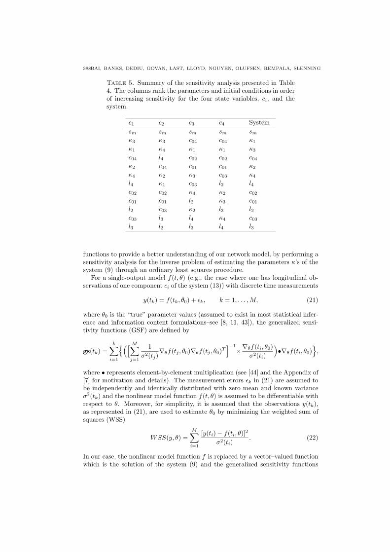
Table 5. Summary of the sensitivity analysis presented in Table4. The columns rank the parameters and initial conditions in orderof increasing sensitivity for the four state variables, ci, and thesystem.
c1 c2 c3 c4 Systemsm sm sm sm sm
κ3 κ3 c04 c04 κ1
κ1 κ4 κ1 κ1 κ3
c04 l4 c02 c02 c04
κ2 c04 c01 c01 κ2
κ4 κ2 κ3 c03 κ4
l4 κ1 c03 l2 l4c02 c02 κ4 κ2 c02
c01 c01 l2 κ3 c01
l2 c03 κ2 l3 l2c03 l3 l4 κ4 c03
l3 l2 l3 l4 l3
functions to provide a better understanding of our network model, by performing asensitivity analysis for the inverse problem of estimating the parameters κ’s of thesystem (9) through an ordinary least squares procedure.
For a single-output model f(t, θ) (e.g., the case where one has longitudinal ob-servations of one component ci of the system (13)) with discrete time measurements
y(tk) = f(tk, θ0) + εk, k = 1, . . . , M, (21)
where θ0 is the “true” parameter values (assumed to exist in most statistical infer-ence and information content formulations–see [8, 11, 43]), the generalized sensi-tivity functions (GSF) are defined by
gs(tk) =k∑
i=1
{([ M∑
j=1
1σ2(tj)
∇θf(tj , θ0)∇θf(tj , θ0)T]−1
×∇θf(ti, θ0)σ2(ti)
)•∇θf(ti, θ0)
},
where • represents element-by-element multiplication (see [44] and the Appendix of[7] for motivation and details). The measurement errors εk in (21) are assumed tobe independently and identically distributed with zero mean and known varianceσ2(tk) and the nonlinear model function f(t, θ) is assumed to be differentiable withrespect to θ. Moreover, for simplicity, it is assumed that the observations y(tk),as represented in (21), are used to estimate θ0 by minimizing the weighted sum ofsquares (WSS)
WSS(y, θ) =M∑
i=1
[y(ti)− f(ti, θ)]2
σ2(ti). (22)
In our case, the nonlinear model function f is replaced by a vector–valued functionwhich is the solution of the system (9) and the generalized sensitivity functions
MODELS FOR AGRICULTURAL PRODUCTION NETWORKS 389
(GSF) are given by
gs(tk) =k∑
i=1
4∑
l=1
{([ M∑
j=1
4∑
l=1
1σ2
l (tj)∇θcl(tj , θ0)∇θcl(tj , θ0)T
]−1
× ∇θcl(ti, θ0)σ2
l (ti)
)• ∇θcl(ti, θ0)
}.
(23)
Here ∇θcl represents the gradient of the state variable cl with respect to θ, whereθ ∈ RP is a vector including all (or just a subset of) the parameters κ’s and l’s andthe initial conditions c0’s.
We note that the generalized sensitivity functions (23) are vector-valued func-tions having the same dimension P as θ and defined only at the discrete time pointstk, k = 1, . . . ,M . They are cumulative functions, at each time point tk taking intoaccount only the contributions of the measurements up to tk, thus representing theinfluence of longitudinal measurements in contributing to the parameter estimates.
From (23) it follows that all the components of gs are one at the end of theexperiment; i.e., gs(tM ) = 1. If one defines gs(t) = 0 for t < t1 (gs is zero whenno measurement is collected) and interpolates gs continuously between observationtimes, then each component gsp of gs varies continuously from 0 to 1 during theexperiment. As we will see in the example below, this transition is not necessarilymonotonic (gsp, p = 1, . . . , P may have oscillations) nor is it restricted to values in[0, 1] (i.e., gsp may take values outside [0, 1]) if large correlations between parameterestimates exist. As discussed in [44], the time subinterval during which this transi-tion has the sharpest increase corresponds to measurements which provide the mostinformation on possible variations in the corresponding true model parameters.
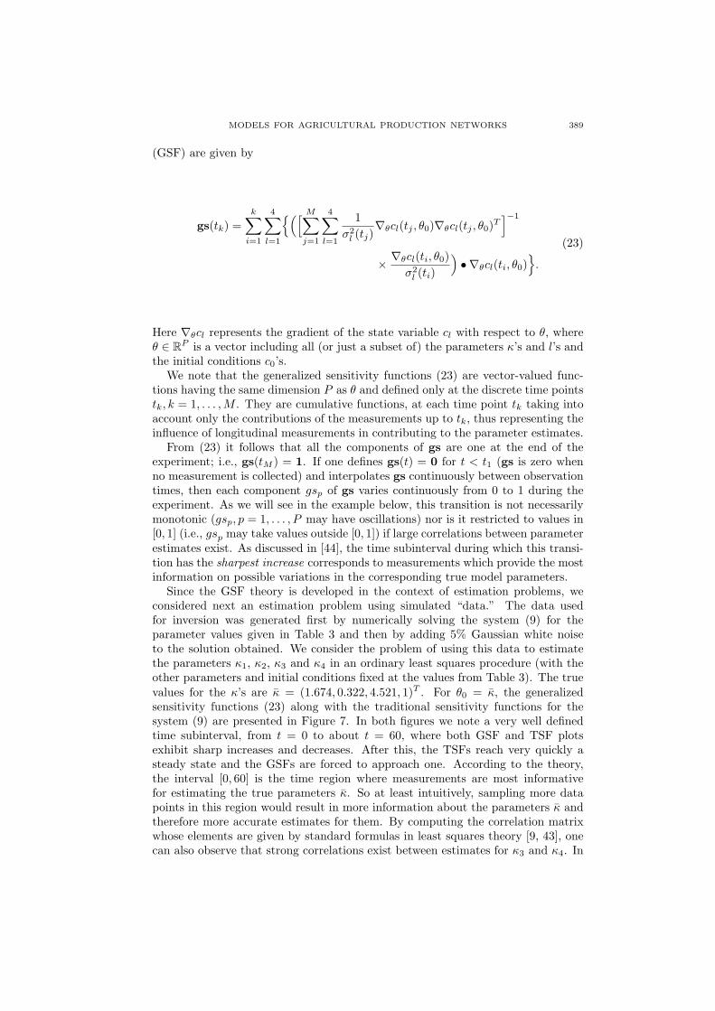
Since the GSF theory is developed in the context of estimation problems, weconsidered next an estimation problem using simulated “data.” The data usedfor inversion was generated first by numerically solving the system (9) for theparameter values given in Table 3 and then by adding 5% Gaussian white noiseto the solution obtained. We consider the problem of using this data to estimatethe parameters κ1, κ2, κ3 and κ4 in an ordinary least squares procedure (with theother parameters and initial conditions fixed at the values from Table 3). The truevalues for the κ’s are κ = (1.674, 0.322, 4.521, 1)T . For θ0 = κ, the generalizedsensitivity functions (23) along with the traditional sensitivity functions for thesystem (9) are presented in Figure 7. In both figures we note a very well definedtime subinterval, from t = 0 to about t = 60, where both GSF and TSF plotsexhibit sharp increases and decreases. After this, the TSFs reach very quickly asteady state and the GSFs are forced to approach one. According to the theory,the interval [0, 60] is the time region where measurements are most informativefor estimating the true parameters κ. So at least intuitively, sampling more datapoints in this region would result in more information about the parameters κ andtherefore more accurate estimates for them. By computing the correlation matrixwhose elements are given by standard formulas in least squares theory [9, 43], onecan also observe that strong correlations exist between estimates for κ3 and κ4. In
390BAI, BANKS, DEDIU, GOVAN, LAST, LLOYD, NGUYEN, OLUFSEN, REMPALA, SLENNING
0 50 100 150 200 250−1
−0.5
0
0.5
1
1.5
2
Generalized sensitivity functions with respect to κ1, κ
2,κ
3,κ
4
κ1
κ2
κ3
κ4
0 50 100 150 200 2500
0.1
0.2
0.3
0.4
0.5
0.6
0.7
Traditional sensitivity functions with respect to κ1, κ
2,κ
3,κ
4
κ1
κ2
κ3
κ4
Figure 7. Generalized and traditional sensitivity functions forκ1, κ2, κ3, κ4, employing a simulated data set with M = 210,generated as discussed in the text. Underlying parameter valuesare κ1 = 1.674, κ2 = 0.322, κ4 = 4.521, κ4 = 1, while all otherparameters are as given in Table 3.
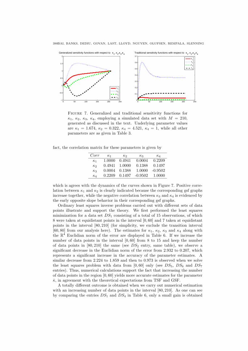
fact, the correlation matrix for these parameters is given by
Corr κ1 κ2 κ3 κ4
κ1 1.0000 0.4941 0.0004 0.2209κ2 0.4941 1.0000 0.1388 0.1497κ3 0.0004 0.1388 1.0000 -0.9502κ4 0.2209 0.1497 -0.9502 1.0000
which is agrees with the dynamics of the curves shown in Figure 7. Positive corre-lation between κ1 and κ2 is clearly indicated because the corresponding gsf graphsincrease together, while the negative correlation between κ3 and κ4 is evidenced bythe early opposite slope behavior in their corresponding gsf graphs.
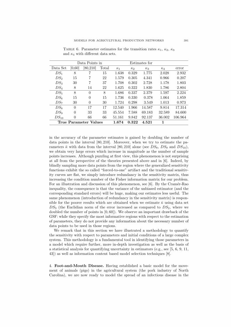
Ordinary least squares inverse problems carried out with different sets of datapoints illustrate and support the theory. We first performed the least squaresminimization for a data set DS1 consisting of a total of 15 observations, of which8 were taken at equidistant points in the interval [0, 60] and 7 taken at equidistantpoints in the interval [80, 210] (for simplicity, we exclude the transition interval[60, 80] from our analysis here). The estimates for κ1, κ2, κ3 and κ4 along withthe R4 Euclidian norm of the error are displayed in Table 6. If we increase thenumber of data points in the interval [0, 60] from 8 to 15 and keep the numberof data points in [80, 210] the same (see DS2 entry, same table), we observe asignificant decrease in the Euclidian norm of the error from 2.932 to 0.207, whichrepresents a significant increase in the accuracy of the parameter estimates. Asimilar decrease from 2.224 to 1.859 and then to 0.973 is observed when we solvethe least squares problem with data from [0, 60] only (see DS5, DS6 and DS7
entries). Thus, numerical calculations support the fact that increasing the numberof data points in the region [0, 60] yields more accurate estimates for the parameterκ, in agreement with the theoretical expectations from TSF and GSF.
A totally different outcome is obtained when we carry out numerical estimationwith an increasing number of data points in the interval [80, 210]. As one can seeby comparing the entries DS1 and DS4 in Table 6, only a small gain is obtained
MODELS FOR AGRICULTURAL PRODUCTION NETWORKS 391
Table 6. Parameter estimates for the transition rates κ1, κ2, κ3
and κ4 with different data sets.
Data Points in Estimates forData Set [0,60] [80,210] Total κ1 κ2 κ3 κ4 error
DS1 8 7 15 1.638 0.329 1.775 2.028 2.932DS2 15 7 22 1.579 0.305 4.341 0.966 0.207DS3 30 7 37 1.708 0.302 2.728 1.178 1.803DS4 8 14 22 1.625 0.322 1.830 1.786 2.804DS5 8 0 8 1.686 0.337 2.379 1.597 2.224DS6 15 0 15 1.736 0.330 0.378 1.064 1.859DS7 30 0 30 1.724 0.298 3.549 1.013 0.973DS8 0 17 17 12.540 1.966 14.587 9.814 17.314DS9 0 33 33 45.554 7.588 69.183 32.589 84.600DS10 0 66 66 51.161 9.842 92.137 36.002 106.964
True Parameter Values 1.674 0.322 4.521 1
in the accuracy of the parameter estimates is gained by doubling the number ofdata points in the interval [80, 210]. Moreover, when we try to estimate the pa-rameters κ with data from the interval [80, 210] alone (see DS8, DS9 and DS10),we obtain very large errors which increase in magnitude as the number of samplepoints increases. Although puzzling at first view, this phenomenon is not surprisingat all from the perspective of the theories presented above and in [6]. Indeed, byblindly sampling more data points from the region where the generalized sensitivityfunctions exhibit the so called “forced-to-one” artifact and the traditional sensitiv-ity curves are flat, we simply introduce redundancy in the sensitivity matrix, thusincreasing the condition number of the Fisher information matrix for our problem.For an illustration and discussion of this phenomenon, see [6]. By the Cramer-Raoinequality, the consequence is that the variance of the unbiased estimator (and thecorresponding standard errors) will be huge, making our estimates less useful. Thesame phenomenon (introduction of redundancy in the sensitivity matrix) is respon-sible for the poorer results which are obtained when we estimate κ using data setDS3 (the Euclidian norm of the error increased as compared to DS2, where wedoubled the number of points in [0, 60]). We observe an important drawback of theGSF: while they specify the most informative regions with respect to the estimationof parameters, they do not provide any information about the necessary number ofdata points to be used in those regions.
We remark that in this section we have illustrated a methodology to quantifythe sensitivity with respect to parameters and initial conditions of a large complexsystem. This methodology is a fundamental tool in identifying those parameters ina model which require further, more in-depth investigation as well as the basis ofa statistical analysis for quantifying uncertainty in estimators (e.g., see [5, 6, 9, 11,43]) as well as information content based model selection techniques [8].
4. Foot-and-Mouth Disease. Having established a basic model for the move-ment of animals (pigs) in the agricultural system (the pork industry of NorthCarolina), we are now ready to model the spread of an infectious disease in the
392BAI, BANKS, DEDIU, GOVAN, LAST, LLOYD, NGUYEN, OLUFSEN, REMPALA, SLENNING
food production network. In this section we describe the incorporation of an SIR-type infection into the system and present simulations to illustrate the spread offoot-and-mouth disease throughout the aggregated agricultural network.
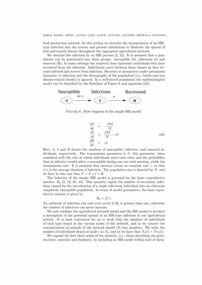
We describe the infection by an SIR process [2, 12]. It is assumed that a pop-ulation can be partitioned into three groups: susceptible (S), infectious (I) andremoved (R). In many settings the removed class represents individuals who haverecovered from the infection. Individuals move between these classes as they be-come infected and recover from infection. Recovery is assumed to confer permanentimmunity to infection and the demography of the population (i.e., births and nondisease-related deaths) is ignored. In a well-mixed population the epidemiologicalmodel can be described by the flowchart of Figure 8 and equations (24).
Susceptible
RIS
Infectious Recoveredγ Iβ SI / N
Figure 8. Flow diagram of the simple SIR model.
dS
dt= −βSI
NdI
dt=
βSI
N− γI (24)
dR
dt= γI.
Here, S, I and R denote the numbers of susceptible, infective, and removed in-dividuals, respectively. The transmission parameter is β: this parameter, whencombined with the rate at which individuals meet each other and the probabilitythat an infective would infect a susceptible during any one such meeting, yields thetransmission rate. It is assumed that recovery occurs at constant rate γ, so that1/γ is the average duration of infection. The population size is denoted by N , andwe have in this case that N = S + I + R.
The behavior of the simple SIR model is governed by the basic reproductivenumber, R0 [2, 12, 31, 14]. This quantity equals the number of secondary infec-tions caused by the introduction of a single infectious individual into an otherwisecompletely susceptible population. In terms of model parameters, the basic repro-ductive number is given by
R0 = β/γ.
An outbreak of infection can only ever occur if R0 is greater than one, otherwisethe number of infectives can never increase.
We now combine the agricultural network model and the SIR model to producea description of the potential spread of an SIR-type infection in our agriculturalsystem. It is most convenient for us to work with the numbers of individualsof each type found at the various nodes of the network, and so we convert theconcentrations of animals of the network model (9) into numbers. We write thenumber of individuals found at node i as Ni, and so we have that Ni(t) = Nci(t).
We expand the first three nodes of the network, (i.e., those describing the grow-ers/sows, nurseries and finishers), by including an SIR model within each of them.
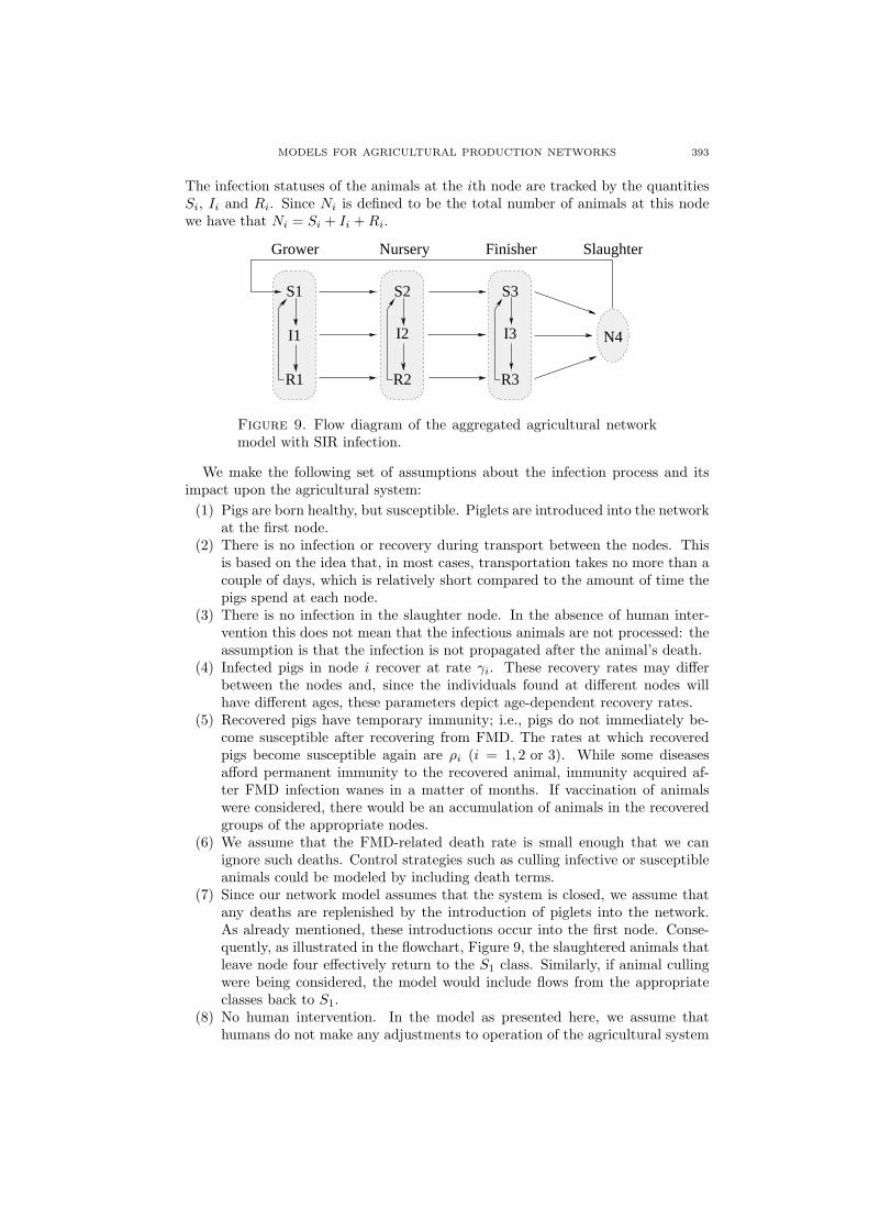
MODELS FOR AGRICULTURAL PRODUCTION NETWORKS 393
The infection statuses of the animals at the ith node are tracked by the quantitiesSi, Ii and Ri. Since Ni is defined to be the total number of animals at this nodewe have that Ni = Si + Ii + Ri.
I3 N4
NurseryGrower SlaughterFinisher
S1
I1
S2
R1
I2
R2
S3
R3
Figure 9. Flow diagram of the aggregated agricultural networkmodel with SIR infection.
We make the following set of assumptions about the infection process and itsimpact upon the agricultural system:
(1) Pigs are born healthy, but susceptible. Piglets are introduced into the networkat the first node.
(2) There is no infection or recovery during transport between the nodes. Thisis based on the idea that, in most cases, transportation takes no more than acouple of days, which is relatively short compared to the amount of time thepigs spend at each node.
(3) There is no infection in the slaughter node. In the absence of human inter-vention this does not mean that the infectious animals are not processed: theassumption is that the infection is not propagated after the animal’s death.
(4) Infected pigs in node i recover at rate γi. These recovery rates may differbetween the nodes and, since the individuals found at different nodes willhave different ages, these parameters depict age-dependent recovery rates.
(5) Recovered pigs have temporary immunity; i.e., pigs do not immediately be-come susceptible after recovering from FMD. The rates at which recoveredpigs become susceptible again are ρi (i = 1, 2 or 3). While some diseasesafford permanent immunity to the recovered animal, immunity acquired af-ter FMD infection wanes in a matter of months. If vaccination of animalswere considered, there would be an accumulation of animals in the recoveredgroups of the appropriate nodes.
(6) We assume that the FMD-related death rate is small enough that we canignore such deaths. Control strategies such as culling infective or susceptibleanimals could be modeled by including death terms.
(7) Since our network model assumes that the system is closed, we assume thatany deaths are replenished by the introduction of piglets into the network.As already mentioned, these introductions occur into the first node. Conse-quently, as illustrated in the flowchart, Figure 9, the slaughtered animals thatleave node four effectively return to the S1 class. Similarly, if animal cullingwere being considered, the model would include flows from the appropriateclasses back to S1.
(8) No human intervention. In the model as presented here, we assume thathumans do not make any adjustments to operation of the agricultural system
394BAI, BANKS, DEDIU, GOVAN, LAST, LLOYD, NGUYEN, OLUFSEN, REMPALA, SLENNING
in response to the infection: animal movement and processing continues asnormal. Of course, one of the main aims of creating a model such as this is toenable the consideration of control strategies. In this study, we do not do thisas we wish to first establish the baseline (no-control) behavior of the system.
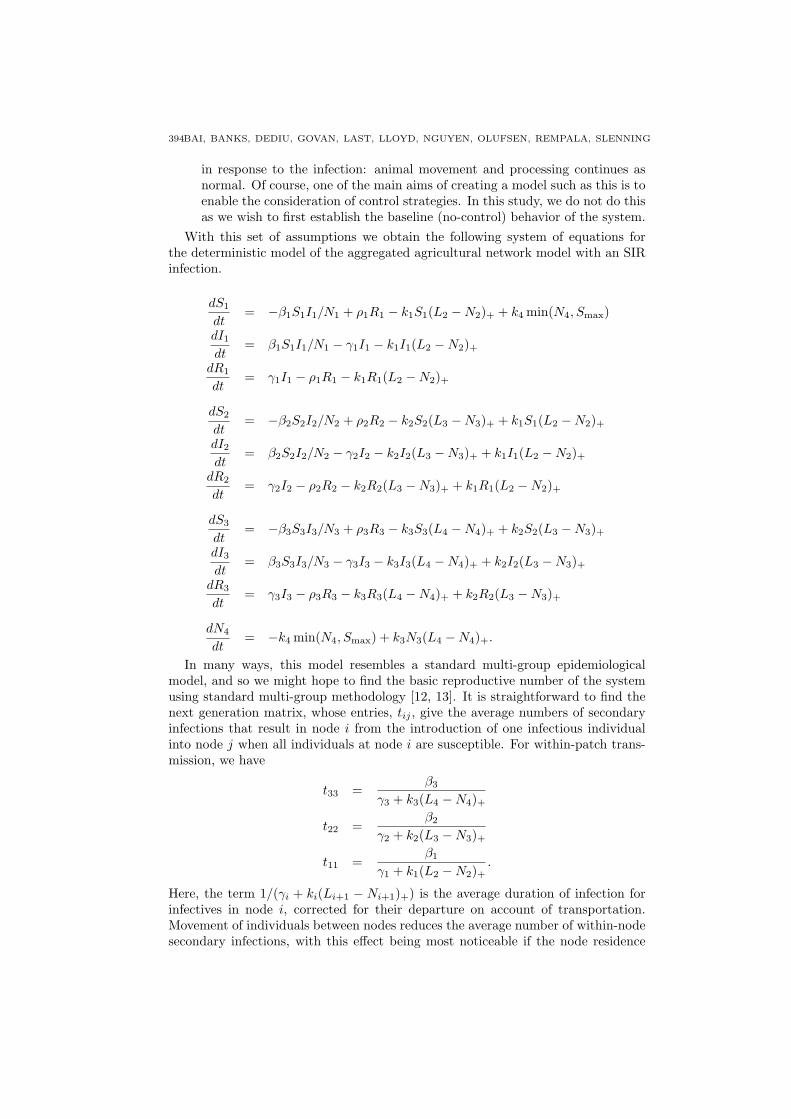
With this set of assumptions we obtain the following system of equations forthe deterministic model of the aggregated agricultural network model with an SIRinfection.
dS1
dt= −β1S1I1/N1 + ρ1R1 − k1S1(L2 −N2)+ + k4 min(N4, Smax)
dI1
dt= β1S1I1/N1 − γ1I1 − k1I1(L2 −N2)+
dR1
dt= γ1I1 − ρ1R1 − k1R1(L2 −N2)+
dS2
dt= −β2S2I2/N2 + ρ2R2 − k2S2(L3 −N3)+ + k1S1(L2 −N2)+
dI2
dt= β2S2I2/N2 − γ2I2 − k2I2(L3 −N3)+ + k1I1(L2 −N2)+
dR2
dt= γ2I2 − ρ2R2 − k2R2(L3 −N3)+ + k1R1(L2 −N2)+
dS3
dt= −β3S3I3/N3 + ρ3R3 − k3S3(L4 −N4)+ + k2S2(L3 −N3)+
dI3
dt= β3S3I3/N3 − γ3I3 − k3I3(L4 −N4)+ + k2I2(L3 −N3)+
dR3
dt= γ3I3 − ρ3R3 − k3R3(L4 −N4)+ + k2R2(L3 −N3)+
dN4
dt= −k4 min(N4, Smax) + k3N3(L4 −N4)+.
In many ways, this model resembles a standard multi-group epidemiologicalmodel, and so we might hope to find the basic reproductive number of the systemusing standard multi-group methodology [12, 13]. It is straightforward to find thenext generation matrix, whose entries, tij , give the average numbers of secondaryinfections that result in node i from the introduction of one infectious individualinto node j when all individuals at node i are susceptible. For within-patch trans-mission, we have
t33 =β3
γ3 + k3(L4 −N4)+
t22 =β2
γ2 + k2(L3 −N3)+
t11 =β1
γ1 + k1(L2 −N2)+.
Here, the term 1/(γi + ki(Li+1 − Ni+1)+) is the average duration of infection forinfectives in node i, corrected for their departure on account of transportation.Movement of individuals between nodes reduces the average number of within-nodesecondary infections, with this effect being most noticeable if the node residence
MODELS FOR AGRICULTURAL PRODUCTION NETWORKS 395
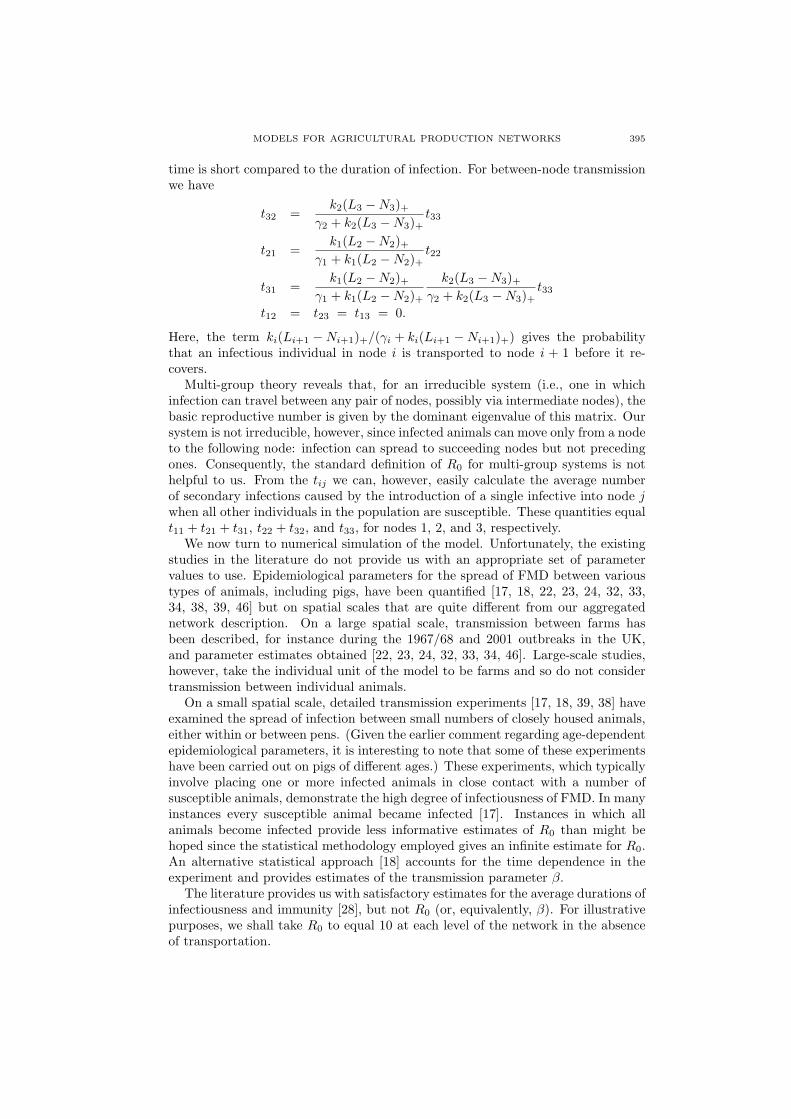
time is short compared to the duration of infection. For between-node transmissionwe have
t32 =k2(L3 −N3)+
γ2 + k2(L3 −N3)+t33
t21 =k1(L2 −N2)+
γ1 + k1(L2 −N2)+t22
t31 =k1(L2 −N2)+
γ1 + k1(L2 −N2)+k2(L3 −N3)+
γ2 + k2(L3 −N3)+t33
t12 = t23 = t13 = 0.
Here, the term ki(Li+1 −Ni+1)+/(γi + ki(Li+1 −Ni+1)+) gives the probabilitythat an infectious individual in node i is transported to node i + 1 before it re-covers.
Multi-group theory reveals that, for an irreducible system (i.e., one in whichinfection can travel between any pair of nodes, possibly via intermediate nodes), thebasic reproductive number is given by the dominant eigenvalue of this matrix. Oursystem is not irreducible, however, since infected animals can move only from a nodeto the following node: infection can spread to succeeding nodes but not precedingones. Consequently, the standard definition of R0 for multi-group systems is nothelpful to us. From the tij we can, however, easily calculate the average numberof secondary infections caused by the introduction of a single infective into node jwhen all other individuals in the population are susceptible. These quantities equalt11 + t21 + t31, t22 + t32, and t33, for nodes 1, 2, and 3, respectively.
We now turn to numerical simulation of the model. Unfortunately, the existingstudies in the literature do not provide us with an appropriate set of parametervalues to use. Epidemiological parameters for the spread of FMD between varioustypes of animals, including pigs, have been quantified [17, 18, 22, 23, 24, 32, 33,34, 38, 39, 46] but on spatial scales that are quite different from our aggregatednetwork description. On a large spatial scale, transmission between farms hasbeen described, for instance during the 1967/68 and 2001 outbreaks in the UK,and parameter estimates obtained [22, 23, 24, 32, 33, 34, 46]. Large-scale studies,however, take the individual unit of the model to be farms and so do not considertransmission between individual animals.
On a small spatial scale, detailed transmission experiments [17, 18, 39, 38] haveexamined the spread of infection between small numbers of closely housed animals,either within or between pens. (Given the earlier comment regarding age-dependentepidemiological parameters, it is interesting to note that some of these experimentshave been carried out on pigs of different ages.) These experiments, which typicallyinvolve placing one or more infected animals in close contact with a number ofsusceptible animals, demonstrate the high degree of infectiousness of FMD. In manyinstances every susceptible animal became infected [17]. Instances in which allanimals become infected provide less informative estimates of R0 than might behoped since the statistical methodology employed gives an infinite estimate for R0.An alternative statistical approach [18] accounts for the time dependence in theexperiment and provides estimates of the transmission parameter β.
The literature provides us with satisfactory estimates for the average durations ofinfectiousness and immunity [28], but not R0 (or, equivalently, β). For illustrativepurposes, we shall take R0 to equal 10 at each level of the network in the absenceof transportation.
396BAI, BANKS, DEDIU, GOVAN, LAST, LLOYD, NGUYEN, OLUFSEN, REMPALA, SLENNING
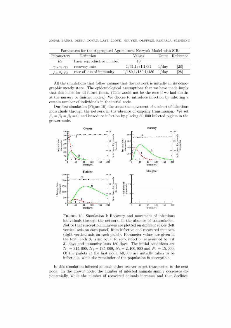
Parameters for the Aggregated Agricultural Network Model with SIRParameters Definition Values Units Reference
R0 basic reproductive number 10γ1, γ2, γ3 recovery rate 1/31,1/31,1/31 1/day [28]ρ1, ρ2, ρ3 rate of loss of immunity 1/180,1/180,1/180 1/day [28]
All the simulations that follow assume that the network is initially in its demo-graphic steady state. The epidemiological assumptions that we have made implythat this holds for all future times. (This would not be the case if we had deathsat the nursery or finisher nodes.) We choose to introduce infection by infecting acertain number of individuals in the initial node.
Our first simulation (Figure 10) illustrates the movement of a cohort of infectiousindividuals through the network in the absence of ongoing transmission. We setβ1 = β2 = β3 = 0, and introduce infection by placing 50, 000 infected piglets in thegrower node.
0 40 80 120 160 200time (days)
0
50
100
150
200
250
300
350
Susc
eptib
les
(t
hous
ands
)
Grower
0 40 80 120 160 200time (days)
0
200
400
600
800
Susc
eptib
les
(t
hous
ands
)Nursery
0 40 80 120 160 200time (days)
0
500
1000
1500
2000
2500
Susc
eptib
les
(th
ousa
nds)
Finisher
0 40 80 120 160 200time (days)
0
10
20
30
Tot
al n
umbe
r
(th
ousa
nds)
Slaughter
0 40 80 120 160 200time (days)
0
10
20
30
Infe
ctiv
es, R
ecov
ered
s
(t
hous
ands
)
Grower
0 40 80 120 160 200time (days)
0
10
20
30
Infe
ctiv
es, R
ecov
ered
s
(
thou
sand
s)
Nursery
0 40 80 120 160 200time (days)
0
10
20
30
Infe
ctiv
es, R
ecov
ered
s
(
thou
sand
s)
Finisher
S S
S
I
I
I
R
R
R
Figure 10. Simulation I: Recovery and movement of infectiousindividuals through the network, in the absence of transmission.Notice that susceptible numbers are plotted on different scales (leftvertical axis on each panel) from infective and recovered numbers(right vertical axis on each panel). Parameter values are given inthe text: each βi is set equal to zero, infection is assumed to last31 days and immunity lasts 180 days. The initial conditions areN1 = 315, 000, N2 = 735, 000, N3 = 2, 100, 000 and N4 = 15, 000.Of the piglets at the first node, 50, 000 are initially taken to beinfectious, while the remainder of the population is susceptible.
In this simulation infected animals either recover or get transported to the nextnode. In the grower node, the number of infected animals simply decreases ex-ponentially, while the number of recovered animals increases and then declines.
MODELS FOR AGRICULTURAL PRODUCTION NETWORKS 397
Within a fairly short time period, the grower population is entirely replaced bysusceptible individuals, reflecting the rapid turnover of the grower node. We seethe appearance of infection first at the nursery and then at the finisher node. Sincethe system is at demographic equilibrium, we see no change at the slaughter node.
For our second simulation (Figure 11), we assume that, in the absence of trans-portation, the infection would have a basic reproductive number equal to 10 at eachnode. Consequently, we set βi/γi = 10. As before, we take the initial populationto be in demographic equilibrium, but we now introduce just 200 infective pigletsinto the grower node.
0 50 100 150 200time (days)
0
50
100
150
200
250
300
Num
ber
of p
igs
(t
hous
ands
)
Grower
0 50 100 150 200time (days)
0
200
400
600
800
Num
ber
of p
igs
(t
hous
ands
)
Nursery
0 50 100 150 200time (days)
0
500
1000
1500
2000
2500
Num
ber
of p
igs
(t
hous
ands
)
Finisher
S S
S
II
I
R
R
R
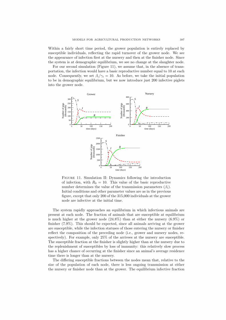
Figure 11. Simulation II: Dynamics following the introductionof infection, with R0 = 10. This value of the basic reproductivenumber determines the value of the transmission parameters (βi).Initial conditions and other parameter values are as in the previousfigure, except that only 200 of the 315,000 individuals at the growernode are infective at the initial time.
The system rapidly approaches an equilibrium in which infectious animals arepresent at each node. The fraction of animals that are susceptible at equilibriumis much higher at the grower node (24.8%) than at either the nursery (6.9%) orfinisher (7.9%). This should be expected, since all animals arriving at the growerare susceptible, while the infection statuses of those entering the nursery or finisherreflect the composition of the preceding node (i.e., grower and nursery nodes, re-spectively). For example, only 25% of the arrivees at the nursery are susceptible.The susceptible fraction at the finisher is slightly higher than at the nursery due tothe replenishment of susceptibles by loss of immunity: this relatively slow processhas a higher chance of occurring at the finisher since an animal’s average residencetime there is longer than at the nursery.
The differing susceptible fractions between the nodes mean that, relative to thesize of the population of each node, there is less ongoing transmission at eitherthe nursery or finisher node than at the grower. The equilibrium infective fraction
398BAI, BANKS, DEDIU, GOVAN, LAST, LLOYD, NGUYEN, OLUFSEN, REMPALA, SLENNING
decreases as the supply chain is traversed (46.8%, 31.5% and 16.2% at the grower,nursery and finisher, respectively), while the recovered fraction increases (28.4%,61.5% and 75.9%).
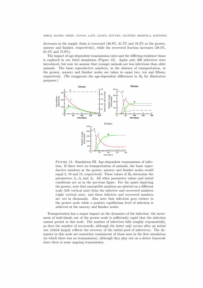
The impact of age-dependent transmission rates and the differing residence timesis explored in our third simulation (Figure 12). Again only 200 infectives wereintroduced, but now we assume that younger animals are less infectious than olderanimals. The basic reproductive numbers, in the absence of transportation, atthe grower, nursery and finisher nodes are taken to equal two, ten and fifteen,respectively. (We exaggerate the age-dependent differences in R0 for illustrativepurposes.)
0 50 100 150 200time (days)
0
100
200
300
Susc
eptib
les
(th
ousa
nds)
Grower
0 50 100 150 200time (days)
0
200
400
600
800
Num
ber
of p
igs
(t
hous
ands
)
Nursery
0 50 100 150 200time (days)
0
500
1000
1500
2000
2500
Num
ber
of p
igs
(t
hous
ands
)
Finisher
0 50 100 150 200time (days)
0
50
100
150
200
250
Infe
ctiv
es, R
ecov
ered
s
Grower
0 50 100 150 200time (days)
Nursery
S S
S
II
I
R
R
R
Figure 12. Simulation III. Age-dependent transmission of infec-tion. If there were no transportation of animals, the basic repro-ductive numbers at the grower, nursery and finisher nodes wouldequal 2, 10 and 15, respectively. These values of R0 determine theparameters β1, β2 and β3. All other parameter values and initialconditions are as in the previous figure. For the panel depictingthe grower, note that susceptible numbers are plotted on a differentscale (left vertical axis) from the infective and recovered numbers(right vertical axis), and these infective and recovered numbersare not in thousands. Also note that infection goes extinct inthe grower node while a positive equilibrium level of infection isachieved at the nursery and finisher nodes.
Transportation has a major impact on the dynamics of the infection: the move-ment of individuals out of the grower node is sufficiently rapid that the infectioncannot persist in this node. The number of infectives falls roughly exponentially,as does the number of recovereds, although the latter only occurs after an initialrise (which largely reflects the recovery of the initial pool of infectives). The dy-namics in this node are somewhat reminiscent of those seen in the first simulation(in which there was no transmission), although they play out on a slower timescalesince there is some ongoing transmission.
MODELS FOR AGRICULTURAL PRODUCTION NETWORKS 399
Disease transmission at the nursery and finisher nodes occurs sufficiently fastthat the prevalence of infection approaches a positive, endemic, equilibrium at both.Observe that, even though the transmission parameter in the nursery node is thesame as it was in the previous simulation, the equilibrium numbers of susceptiblesand infectives are higher here than they were in the previous simulation. Thisreflects the differences between the compositions of the populations entering thenursery node in the two simulations, with more susceptibles arriving in the age-dependent situation.
5. Concluding Remarks. In this paper we have demonstrated a methodologicalapproach to the investigation of production networks and their vulnerability todisturbances such as diseases. The stochastic model and the resulting approximatedeterministic system we employ were shown to agree well, but are not validated.Rather, we carry out simulations and sensitivity analyses with parameter valuesthat are only loosely based on a swine network. We use the deterministic modelto show how to determine the parameters to which the model at these parametervalues exhibits the most sensitivity. Finally, we demonstrate how disease can beintroduced and the resulting network vulnerabilities analyzed. An interesting nextstep would involve obtaining experimental data to validate and perhaps improve themodel for a specific production network. This would require using inverse problemalgorithms with the data to obtain estimates along with measures of associateduncertainty (e.g., standard errors [9, 43]) for the underlying transition rates ki.
Other obvious questions for further investigation involve the transmission dy-namics of the infection. It is well known, for example, that random effects canhave a major impact on the invasion of an infection into a population. The useof constant rates of recovery and loss of immunity for the infection should also bequestioned. These assumptions, which are biologically unrealistic for many infec-tions, could be important in cases such as the one presented above where the lifespan of the animals is comparable in length to the duration of infection and immu-nity. Finally, the model used here assumes instantaneous transport between nodes.If infection during transport is an important factor (and depending on the diseaseit may well be) then the structure of the model should be modified to incorporatepositive transport times. This could lead to more interesting (mathematically) andmore difficult dynamical systems with time delays in place of (9) and the corre-sponding systems in Section 4.
The randomness seen in the stochastic network model originates from the ran-dom movement of discrete individuals from node to node. The analysis of Sections2.2 and 3.2 shows that, due to an averaging effect, these random effects becomeless important as the system size N increases. Application of the stochastic trans-portation model to describe a real-world situation should, therefore, account forthe size of the groups in which pigs are transported between nodes. If, for example,one thousand pigs were moved at a time, the appropriate notion of an “individual”within the model would be a thousand pigs. Treating each group of a thousandanimals as a unit would lead to a marked increase in the magnitude of stochasticfluctuations seen at the population level. Consequently, even though the systemsize in our simulations is on the order of millions of pigs, it might be that the re-sulting stochastic fluctuations in a more realistic model of the production systemare closer to those shown in Figure 3 than to those of Figure 2.
400BAI, BANKS, DEDIU, GOVAN, LAST, LLOYD, NGUYEN, OLUFSEN, REMPALA, SLENNING
The approach outlined in this paper has rather obvious potential for applicationto a wide range of problems. These include the investigation of the spread ofdiseases through spatially or structurally distributed dynamic populations (e.g.,avian flu through migrating bird populations, contagious infections through humanand animal populations that are highly mobile, highly age-structured, or both). Insome of these cases the natural nodal structure would be a continuum, requiringstochastic and deterministic models with a continuum of spatial and structuralheterogeneities, leading to partial differential equation systems. Such applicationswould undoubtedly motivate the development of interesting new stochastic anddeterministic mathematical and computational methodologies.
We also note that the approach and methodology presented here are useful forinvestigation of a wide range of perturbations other than disease (e.g., loss of ca-pacity at a given node such as a factory being shut down for some reason) in supplynetworks. In particular they would be useful in the assessment of risk of a food-borne pathogen (e.g., salmonella, listeria, etc.) entering the food chain [27] due tocontamination (either accidental or deliberate) at some stage of the supply chain.
Acknowledgements. This research was supported in part by the Statistical andApplied Mathematical Sciences Institute, which is funded by NSF under grantDMS-0112069, in part by the National Institute of Allergy and Infectious Diseaseunder grant 9R01AI071915-05, and in part by the U.S. Air Force Office of ScientificResearch under grant AFOSR-FA9550-04-1-0220.
REFERENCES
[1] G. Almond (College of Veterinary Medicine, NC State University), R. Baker (College ofVeterinary Medicine, Iowa State University), M. Battrell (Murphy Farms, NC), J. Tickel(Emergency Programs, NC Dept of Agriculture and Consumer Services), personal communi-cations.
[2] R. M. Anderson and R. M. May, Infectious Diseases of Humans: Dynamics and Control,Oxford University Press, Oxford, 1991.
[3] H. Andersson and T. Britton, Stochastic Epidemic Models and Their Statistical Analysis,Lec Notes in Statistics, 151, Springer Verlag, New York, 2000.
[4] H. T. Banks, S. Dediu and S.L. Ernstberger, Sensitivity functions and their use in inverseproblems, to appear.
[5] H. T. Banks, S. Dediu and H.K. Nguyen, Sensitivity of dynamical systems to parameters ina convex subset of a topological vector space, Center for Research in Scientific ComputationReport, CRSC-TR06-25, September, 2006, North Carolina State University; Math. Biosci.and Engineering, submitted.
[6] H. T. Banks, S.L. Ernstberger and S.L. Grove, Standard errors and confidence intervals ininverse problems: sensitivity and associated pitfalls, CRSC Tech Rep. CRSC-TR06-10, N.C.State University, March, 2006; J. Inverse and Ill-posed Problems, to appear.
[7] J. J. Batzel, F. Kappel, D. Schneditz and H.T. Tran, Cardiovascular and Respiratory Systems:Modeling, Analysis and Control, SIAM Frontiers in Applied Math, SIAM, Philadelphia, 2006.
[8] K. P. Burnham and D. R. Anderson, Model Selection and Multimodel Inference: A PracticalInformation-Theoretic Approach, Springer-Verlag, New York, 2002.
[9] G. Casella and R. L. Berger, Statistical Inference, Duxbury, Pacific Grove, CA, 2002.[10] J.B. Cruz, ed., System Sensitivity Analysis, Dowden, Hutchinson & Ross, Inc., Stroudsberg,
PA, 1973.[11] M. Davidian and D. Giltinan, Nonlinear Models for Repeated Measurement Data, Chapman
& Hall, London, 1998.[12] O. Diekmann and J.A.P. Heesterbeek, Mathematical Epidemiology of Infectious Diseases,
John Wiley & Sons, Chichester, 2000.
MODELS FOR AGRICULTURAL PRODUCTION NETWORKS 401
[13] O. Diekmann, J.A.P. Heesterbeek and J.A.J. Metz, On the definition and computation of thebasic reproduction ratio R0 in models of infectious diseases in heterogeneous populations, J.Math. Biol., 28 (1990), 365–382.
[14] K. Dietz, The estimation of the basic reproductive number for infectious diseases, Stat. Meth.Med. Res., 2 (1993), 23–41.
[15] W. Dorfer-Kreissl, Report of measures to control Foot and Mouth Disease in the EuropeanUnion in 2001 and future measures to prevent and control animal diseases in the EuropeanUnion, European Parliament Session Document A5-0405/2002, 28 Nov 2002, p.45 (para 1,5),p.52 (para 1).
[16] R. Durrett, Essentials of Stochastic Processes, Springer, New York, 1999.[17] P.L. Eble, A. Bouma, M.G. de Bruin, F. van Hemert-Kluitenberg, J.T. van Oirschot and
A. Dekker, Vaccination of pigs two weeks before infection significantly reduces transmissionof foot-and-mouth disease virus, Vaccine, 22 (2004), 1372–1378.
[18] P.L. Eble, A. de Koeijer, A. Bouma, A. Stegeman and A. Dekker, Quantification of within-and between-pen transmission of Foot-and-Mouth disease virus in pigs, Vet. Res., 37 (2006),647–654.
[19] A. El Amin, Round up: Denmark hit by deadly strain of bird flu, FoodProductionDaily.Com-Europe; News Headlines-Supply Chain, 17 Mar 2006, http://www.foodproductiondaily.com/news/ng.asp?id=66483-bird-flu-avian-france
[20] M. Eslami, Theory of Sensitivity in Dynamic Systems: An Introduction, Springer-Verlag,Berlin, 1994.
[21] S. N. Ethier and T. G. Kurtz, Markov Processes: Characterization and Convergence, J. Wiley& Sons, New York, 1986.
[22] N. M. Ferguson, C. A. Donnelly and R. M. Anderson, The foot and mouth epidemic in GreatBritian: Pattern of spread and impact of interventions, Science 292 (2001), 1155–1160.
[23] N. M. Ferguson, C. A. Donnelly and R. M. Anderson, Transmission intensity and impactof control policies on the foot and mouth epidemic in Great Britain, Nature 413 (2001),542–548.
[24] M. J. Ferrari, O. N. Bjørnstad, A. P. Dobson, Estimation and inference of R0 of an infectiouspathogen by a removal method, Math. Biosci., 198 (2005), 14–26.
[25] P.M. Frank, Introduction to System Sensitivity Theory, Academic Press, Inc., New York, NY,1978.
[26] C. Fraser, S. Riley, R. M. Anderson and N. M. Ferguson, Factors that make an infectiousdisease outbreak controllable, Proc. Natl. Acad. Sci. USA 101 (2004), 6146–6151.
[27] M. A. van der Gaag, F. Vos, H. W. Saatkamp, M. van Boven, P. van Beek and R.B.M. Huirne,A state-transition simulation model for the spread of Salmonella in the pork supply chain,European J. Operational Res., 156 (2004), 782–798.
[28] M. G. Garner and M. B. Lack, An evaluation of alternate control strategies for foot-and-mouth disease in Australia: A regional approach, Prev. Vet. Med., 23 (1995), 9–32.
[29] D. T. Gillespie, The chemical Langevin equation, J. Chemical Physics 113 (2000), 297–306.[30] G. R. Grimmett and D. R. Stirzaker, Probability and Random Processes, Clarendon Press,
Oxford, 1982.[31] J. A. P. Heesterbeek, A brief history of R0 and a recipe for its calculation, Acta Biotheor.,
50 (2002), 189–204.[32] D.T. Haydon, M.E.J. Woolhouse and R.P. Kitching, An analysis of foot-and-mouth-disease
epidemics in the UK, IMA J. Math. Appl. Med. Biol., 14 (1997), 1–9.[33] S.C. Howard and C.A. Donnelly, The importance of immediate destruction in epidemics of
foot and mouth disease, Res. Vet. Sci., 69 (2000), 189–196.[34] M.J. Keeling, M.E.J. Woolhouse, D.J. Shaw, L. Matthews, M. Chase-Topping, D.T. Haydon,
S.J. Cornell, J. Kappey, J. Wilesmith and B.T. Grenfell, Dynamics of the 2001 UK foot andmouth epidemic: Stochastic dispersal in a heterogeneous landscape, Science, 294 (2001),813–817.
[35] W. O. Kermack and A. G. McKendrick, A contribution to the mathematical theory of epi-demics, Proc. Roy. Soc. Lond., A 115 (1927), 700–721.
[36] M. Kleiber, H. Antunez, T.D. Hien and P. Kowalczyk, Parameter Sensitivity in NonlinearMechanics: Theory and Finite Element Computations, John Wiley & Sons, New York, NY,1997.
[37] Living Countryside, AgriStats-UK Agriculture-farming statistics, http://www.ukagriculture.com/statistics/farming statistics.cfm.

402BAI, BANKS, DEDIU, GOVAN, LAST, LLOYD, NGUYEN, OLUFSEN, REMPALA, SLENNING
[38] K. Orsel, A. Dekker, A. Bouma, J.A. Stegeman and M.C.M. de Jong, Vaccination againstfoot and mouth disease reduces virus transmission in groups of calves, Vaccine, 23 (2005),4887–4894.
[39] K. Orsel, M.C.M. de Jong, A. Bouma, J.A. Stegeman and A. Dekker, The effect of vaccinationon foot and mouth disease virus transmission among dairy cows, Vaccine, 25 (2007), 327–335.
[40] R: A Language and Environment for Statistical Computing, Foundation for Statistical Com-puting, Vienna, Austria, ISBN 3-900051-07-0.
[41] J. Rushton, T. Willmore, A. Shaw and A. James, Economic analysis of vaccination strategiesfor foot and mouth disease in the UK, Royal Society Inquiry into Infectious Diseases inLivestock, 2002, p21, Tables 3 and 4, http://www.royalsoc.ac.uk/inquiry/index/566.pdf.
[42] A. Saltelli, K. Chan and E.M. Scott, eds., Sensitivity Analysis, Wiley Series in Probabilityand Statistics, John Wiley & Sons, New York, NY, 2000.
[43] G. A. F. Seber and C. J. Wild, Nonlinear Regression, John Wiley & Sons, Inc., New York,1989.
[44] K. Thomaseth and C. Cobelli, Generalized sensitivity functions in physiological system iden-tification, Ann. Biomed Eng., 27 (1999), 607–616.
[45] D. Thompson, P. Muriel, D. Russell, P. Osborne, A. Bromley, M. Rowland, S. Creigh-Tyteand C. Brown, Economic costs of the foot and mouth disease outbreak in the United Kingdomin 2001, Rev. Sci. Tech. Off. Int. Epiz., 21 (2002), 675–687.
[46] M. Woolhouse, M. Chase-Topping, D. Haydon, J. Friar, L. Matthews, G. Hughes, D. Shaw,J. Wilesmith, A. Donaldson, S. Cornell, M. Keeling, and B. Grenfell, Foot-and-mouth diseaseunder control in the UK, Nature 411 (2001), 258–259.
Received on February 23, 2007. Accepted on March 27, 2007.
E-mail address: [email protected]
E-mail address: [email protected](corresponding author)
E-mail address: [email protected]
E-mail address: [email protected]
E-mail address: [email protected]
E-mail address: alun [email protected]
E-mail address: [email protected]
E-mail address: [email protected]
E-mail address: [email protected]
E-mail address: barret [email protected]