Embed Size (px)
Citation preview

The Pennsylvania State University
The Graduate School
Department of Mathematics
STOCHASTIC AND DETERMINISTIC PROCESSES IN
FRAGMENTATION AND SEDIMENTATION
A Dissertation in
Mathematics
by
Michael L. Higley
c© 2010 Michael L. Higley
Submitted in Partial Fulfillmentof the Requirementsfor the Degree of
Doctor of Philosophy
May 2010

The dissertation of Michael L. Higley was approved∗ by the following:
Andrew BelmonteAssociate Professor of MathematicsThesis AdviserChair of Committee
Qiang DuVerne M. Willaman Professor of Mathematics
Diane HendersonProfessor of Mathematics
Francesco CostanzoProfessor of Engineering Science and Mechanics
Gary MullenProfessor of MathematicsHead of the Department of Mathematics
∗Signatures are on file with the Graduate School.

iii
Abstract
In this work we present results of analysis, experiment and simulation of two phe-nomena involving stochastic and deterministic aspects. In the first case we present amodeling framework for 1D fragmentation in brittle rods, in which the distribution offragments is written explicitly in terms of the probability of breaks along the length ofthe rod. This work is motivated by the experimental observation of several preferredlengths in the fragment distribution of shattered brittle rods after dynamic buckling.Our approach allows for non-constant spatial breaking probabilities, which can lead topreferred fragment sizes. The resulting relation is shown to qualitatively match exper-imentally observed fragment distributions, as well as some other commonly reporteddistributions such as a power law with a cutoff.
We also present experimental observations of the trajectories and average ve-locities of solid spheres falling through a curtain of rising bubbles in water. For thequiescent case (no bubbles), the Reynolds numbers are on the order of 1,000, and theaverage terminal velocity is determined by the form (inertial) drag. The main effectof the introduction of bubbles is to slow down the spheres. In some regimes (smalleror lighter spheres), there is an added random lateral motion to the sphere paths. Inthis way, a solid sphere sinking in a bubbly fluid and a solid sphere falling through acrowded bed of rigid obstacles (in air) share two common traits: the settling speed isslowed by the obstructions, and the sphere exhibits random lateral motion. We presenta mathematical model which begins as an adaptation of Galton’s board to the sediment-ing sphere. This allows us to introduce various physical effects of the bubbly fluid, andtest their importance, particularly that of bubble collisions. Comparison is made withexperimental results.

iv
Table of Contents
List of Tables . . . . . . . . . . . . . . . . . . . . . . . . . . . . . . . . . . . . . . vii
List of Figures . . . . . . . . . . . . . . . . . . . . . . . . . . . . . . . . . . . . . viii
Acknowledgments . . . . . . . . . . . . . . . . . . . . . . . . . . . . . . . . . . . xiii
Chapter 1. Fragmentation: introduction . . . . . . . . . . . . . . . . . . . . . . . 1
Chapter 2. Fragmentation: modeling a segmented rod . . . . . . . . . . . . . . . 42.1 Introduction . . . . . . . . . . . . . . . . . . . . . . . . . . . . . . . . 42.2 The combinatorics of breaking . . . . . . . . . . . . . . . . . . . . . . 52.3 Application of Eq. 2.5 to division of a sequence . . . . . . . . . . . . 92.4 Application of Eq. 2.5 to a particular recursive function . . . . . . . 12
Chapter 3. Fragmentation: modeling a continuum rod . . . . . . . . . . . . . . . 163.1 Introduction . . . . . . . . . . . . . . . . . . . . . . . . . . . . . . . . 163.2 Breaking according to a nonhomogenous Poisson process . . . . . . . 163.3 Relation to the segmented rod . . . . . . . . . . . . . . . . . . . . . . 183.4 Properties of the fragment distribution n(`) . . . . . . . . . . . . . . 20
3.4.1 Fragment distributions for several basic λ(x) . . . . . . . . . 203.4.2 Distributions with Power Law Scaling . . . . . . . . . . . . . 24
Chapter 4. Fragmentation: experiment and model comparison . . . . . . . . . . 294.1 Introduction . . . . . . . . . . . . . . . . . . . . . . . . . . . . . . . . 294.2 Experimental Comparisons . . . . . . . . . . . . . . . . . . . . . . . 29
4.2.1 Fitting the previously measured distribution . . . . . . . . . . 294.2.2 Measuring λ(x) experimentally . . . . . . . . . . . . . . . . . 33
4.3 Discussion and Conclusions . . . . . . . . . . . . . . . . . . . . . . . 34
Chapter 5. A sphere sinking in bubbles: introduction . . . . . . . . . . . . . . . 38
Chapter 6. A sphere sinking in bubbles: settling velocity . . . . . . . . . . . . . 446.1 Experimental setup . . . . . . . . . . . . . . . . . . . . . . . . . . . . 44
6.1.1 The container . . . . . . . . . . . . . . . . . . . . . . . . . . . 446.1.2 The bubble field . . . . . . . . . . . . . . . . . . . . . . . . . 446.1.3 The spheres . . . . . . . . . . . . . . . . . . . . . . . . . . . . 496.1.4 Extracting data . . . . . . . . . . . . . . . . . . . . . . . . . . 50
6.2 Findings: terminal velocity in quiescent and bubbly water . . . . . . 546.3 Observations: bubble-sphere interactions . . . . . . . . . . . . . . . . 556.4 Bubble-flow interactions . . . . . . . . . . . . . . . . . . . . . . . . . 56

v
Chapter 7. A sphere sinking in bubbles: collision model . . . . . . . . . . . . . . 627.1 Introduction . . . . . . . . . . . . . . . . . . . . . . . . . . . . . . . . 627.2 The Galton board . . . . . . . . . . . . . . . . . . . . . . . . . . . . 637.3 Examinations and adaptations of the Galton board . . . . . . . . . . 65
7.3.1 Deterministic randomness . . . . . . . . . . . . . . . . . . . . 657.3.2 Dynamical system . . . . . . . . . . . . . . . . . . . . . . . . 687.3.3 An argument for randomness . . . . . . . . . . . . . . . . . . 69
7.4 The fluid Galton model . . . . . . . . . . . . . . . . . . . . . . . . . 727.5 Simulating the fluid Galton model . . . . . . . . . . . . . . . . . . . 72
7.5.1 Adjustable parameters . . . . . . . . . . . . . . . . . . . . . . 727.5.2 Tracer motion . . . . . . . . . . . . . . . . . . . . . . . . . . . 747.5.3 Tracking scatterers . . . . . . . . . . . . . . . . . . . . . . . . 74
7.6 Simulation results . . . . . . . . . . . . . . . . . . . . . . . . . . . . . 757.6.1 Non-dimensionalization of parameters for floating scatterers . 757.6.2 Average settling velocity . . . . . . . . . . . . . . . . . . . . . 767.6.3 Diffusivity . . . . . . . . . . . . . . . . . . . . . . . . . . . . . 767.6.4 Sinking of a heavy sphere in bubbles . . . . . . . . . . . . . . 817.6.5 Autocorrelation . . . . . . . . . . . . . . . . . . . . . . . . . . 85
7.7 Simulation results: added velocity . . . . . . . . . . . . . . . . . . . . 85
Chapter 8. A sphere sinking in bubbles: experimental measurement of collisioneffects . . . . . . . . . . . . . . . . . . . . . . . . . . . . . . . . . . . 90
8.1 Experimental setup . . . . . . . . . . . . . . . . . . . . . . . . . . . . 908.2 Experimental Results . . . . . . . . . . . . . . . . . . . . . . . . . . . 92
8.2.1 Settling Velocity . . . . . . . . . . . . . . . . . . . . . . . . . 928.2.2 Diffusivity . . . . . . . . . . . . . . . . . . . . . . . . . . . . . 938.2.3 Staircasing . . . . . . . . . . . . . . . . . . . . . . . . . . . . 93
Chapter 9. Conclusion and future directions . . . . . . . . . . . . . . . . . . . . 989.0.4 Fragmentation of a 1-D rod . . . . . . . . . . . . . . . . . . . 989.0.5 Spheres sinking in bubbles – a proposed continuum model for
path-clearing . . . . . . . . . . . . . . . . . . . . . . . . . . . 98
Appendix A. Coefficient of restitution . . . . . . . . . . . . . . . . . . . . . . . . 102
Appendix B. A coefficient of restitution for bubbles, drops, and particles . . . . 106B.1 Approach and rebound of two spheres . . . . . . . . . . . . . . . . . 106B.2 Submersed collisions . . . . . . . . . . . . . . . . . . . . . . . . . . . 111B.3 A coefficient of restitution for bubbles and drops . . . . . . . . . . . 114
Appendix C. A modified simulation . . . . . . . . . . . . . . . . . . . . . . . . . 118C.0.1 Modifications . . . . . . . . . . . . . . . . . . . . . . . . . . . 118C.0.2 Comparison of results . . . . . . . . . . . . . . . . . . . . . . 120C.0.3 Comparison with theory . . . . . . . . . . . . . . . . . . . . . 121C.0.4 Eliminating staircasing . . . . . . . . . . . . . . . . . . . . . . 123

vi
Appendix D. Hourglass bubble plumes . . . . . . . . . . . . . . . . . . . . . . . 125D.0.5 The plume . . . . . . . . . . . . . . . . . . . . . . . . . . . . 125D.0.6 Spiraling bubbles . . . . . . . . . . . . . . . . . . . . . . . . . 125D.0.7 Random spirals . . . . . . . . . . . . . . . . . . . . . . . . . . 127
D.1 Conclusions . . . . . . . . . . . . . . . . . . . . . . . . . . . . . . . . 129
References . . . . . . . . . . . . . . . . . . . . . . . . . . . . . . . . . . . . . . . . 139

vii
List of Tables
2.1 The expected number of runs of length i when tossing a fair coin 100 times. 12
4.1 Fitted parameters for the pulses in Eq. 4.1, used for the curves shown inFig. 4.2 . . . . . . . . . . . . . . . . . . . . . . . . . . . . . . . . . . . . 33
6.1 Average properties of the bubble field for 3 ≤ pa ≤ 7 [psi]. . . . . . . . . 506.2 Properties of the spheres used in the first experiment. . . . . . . . . . . 50

viii
List of Figures
1.1 Measured number density of fragments n(`) from [30]. . . . . . . . . . . 3
2.1 A rod (above) goes through an event in which it may break at any of afinite number of locations (joints). An outcome of the event is an orderedcollection of fragments, or equivalently a list of which joints have brokenin the event. In this case we show an outcome in which the rod breaksat the 5th, 6th and 9th joints. . . . . . . . . . . . . . . . . . . . . . . . . 4
2.2 The event space showing all 26 = 64 possible divisions of a rod of J+1 = 7segments in length. . . . . . . . . . . . . . . . . . . . . . . . . . . . . . . 6
2.3 Segments of length 2 occurring in the event space of Fig. 2.2. . . . . . . 72.4 Segments of length 2 within outcomes of Fig. 2.2 having exactly 3 breaks. 82.5 The mapping from a broken rod to a sequence of coin tosses. . . . . . . 102.6 Coin tosses (numbered) and opportunities for breaks (lettered) . . . . . 112.7 Functional dependencies of fk(J + 1, s). Each function depends on all
those below and not to the left of itself. . . . . . . . . . . . . . . . . . . 142.8 Enumeration of calls to fk−N(J + 1− (M +N − 1), s). . . . . . . . . . . 15
3.1 The divisions of a unit rod in which the left end of a fragment of length(`, `+ δ) might occur. . . . . . . . . . . . . . . . . . . . . . . . . . . . . 17
3.2 A fragment with left edge in (x0 + s, x0 + s + dx) and right edge in(x0 + s+ `+ w, x0 + s+ `+ w + dx). . . . . . . . . . . . . . . . . . . . . 18
3.3 Examples of fragment distributions n(`) produced by simple parabolicfunctions. . . . . . . . . . . . . . . . . . . . . . . . . . . . . . . . . . . . 21
3.4 Fragment distributions n(`) produced by λ(x) = A sin2(5πx). . . . . . . 223.5 Fragment distributions n(`) produced by λ(x) = A exp(−100(x − 1
2)2). . 23
3.6 Contributions to n(`) from end and interior fragments. . . . . . . . . . . 243.7 Three evenly spaced pulses in λ(x) produce fewer than 10 peaks in n(`),
as calculated by Eq. 3.12. . . . . . . . . . . . . . . . . . . . . . . . . . . 253.8 Three distinct but incommensurately spaced pulses in λ(x) can produce
10 peaks in n(`), as calculated by Eq. 3.12. . . . . . . . . . . . . . . . . 263.9 Calculated fragment distributions n(`) for power-law λ(x). . . . . . . . . 27
3.10 Fragment distribution n(`) for λ(x) = x−β, β = 1, 1.5, 2, 3. . . . . . . . . 283.11 An example of λ(x) producing scaling over a number of decades. . . . . 28
4.1 Comparison of the model (based on curvature) and experimental data. . 304.2 Comparison of the model (based on six pulses) and experimental data. . 314.3 Comparison of the model (based on nine pulses) and experimental data. 324.4 Experimental images of dynamic buckling and breaking of pasta. . . . . 344.5 Observed patterns in the probability of breaking. . . . . . . . . . . . . . 354.6 Measured values of λ(x). . . . . . . . . . . . . . . . . . . . . . . . . . . . 364.7 Calculated and measured values of n(`). . . . . . . . . . . . . . . . . . . 36

ix
5.1 The standard drag curve from [16] gives the coefficient of drag for Eq. 5.21as a function of a sphere’s Reynolds number. . . . . . . . . . . . . . . . 43
6.1 The first experimental setup for observing a sphere settling in a bubblyfluid. . . . . . . . . . . . . . . . . . . . . . . . . . . . . . . . . . . . . . . 45
6.2 A fully 3D bubble field produced by an array of commercial air stones. . 466.3 Bubble volume flux per centimeter f [cm2/s] as a function of applied
overpressure pa [psi]. The dashed line shows the approximation f =
(1.0pa[psi]− 1.5) cm2/s. . . . . . . . . . . . . . . . . . . . . . . . . . . . 476.4 Bubble number density as a function of applied overpressure. . . . . . . 486.5 Bubble rise velocity as a function of applied overpressure. . . . . . . . . 486.6 Plot of equation 6.1: bubble volume equivalent diameter de [cm] as a
function of applied overpressure pa [psi]. . . . . . . . . . . . . . . . . . . 496.7 Images from an experimental video, 1 of 2. . . . . . . . . . . . . . . . . 526.8 Images from an experimental video, 2 of 2. . . . . . . . . . . . . . . . . 536.9 Measured values of the terminal velocities of spheres in quiescent water. 556.10 Measured values of the terminal velocities of spheres in quiescent water
(black circles) and in bubbles (blue circles) at a variety of pressures. . . 566.11 Paths of sinking spheres. . . . . . . . . . . . . . . . . . . . . . . . . . . . 576.12 Identical spheres – one sinking, one rising. . . . . . . . . . . . . . . . . . 586.13 A bubble is trapped in the wake of a sphere. . . . . . . . . . . . . . . . . 596.14 Bubbles are trapped in the wake of a sphere. . . . . . . . . . . . . . . . 606.15 A sphere and bubble collide. . . . . . . . . . . . . . . . . . . . . . . . . . 606.16 Bubble rise velocity Ub (in red) and water circulation velocity Uw (in
blue) as a function of applied overpressure pa [psi]. . . . . . . . . . . . . 616.17 Measured values of the terminal velocities (cm/s) of spheres in the rest
frame of water circulating in the tank. . . . . . . . . . . . . . . . . . . . 61
7.1 The Barker family pachinko machine (photos by DeeAnne Higley). Apayoff in the game comes when a ball enters one of the receptacles shownin detail to the right. . . . . . . . . . . . . . . . . . . . . . . . . . . . . . 62
7.2 Galton’s board, the quincunx, as he portrayed it [28]. . . . . . . . . . . . 647.3 Probabilities that a tracer will reach given coordinates on the Galton
board. . . . . . . . . . . . . . . . . . . . . . . . . . . . . . . . . . . . . . 657.4 Equivalent Galton boards. . . . . . . . . . . . . . . . . . . . . . . . . . . 667.5 A single jump on the Galton board. . . . . . . . . . . . . . . . . . . . . 707.6 Jump times from θ = π
4 . . . . . . . . . . . . . . . . . . . . . . . . . . . . 717.7 A small change in parameters results in a much different jump. . . . . . 717.8 A sphere-bubble collision. . . . . . . . . . . . . . . . . . . . . . . . . . . 737.9 Sample paths for a tracer of Dt = 0.3 and ρ = 7.2 g/cm3. . . . . . . . . 767.10 Sample paths for a tracer of Dt = 0.3. . . . . . . . . . . . . . . . . . . . 777.11 Average non-dimensionalized settling velocity Vt for a tracer with diam-
eter Dt = 0.3 as a function of density ρ (gm/cm3). . . . . . . . . . . . . 787.12 Average non-dimensionalized settling velocity Vt as a function of density
ρ [gm/cm3]. . . . . . . . . . . . . . . . . . . . . . . . . . . . . . . . . . 78

x
7.13 Transition density ρt [gm/cm3] as a function of non-dimensionalized di-ameter Dt. . . . . . . . . . . . . . . . . . . . . . . . . . . . . . . . . . . 79
7.14 Average settling velocity Vt for a tracer with Dt = 0.4 as a function ofdensity ρ (gm/cm3). . . . . . . . . . . . . . . . . . . . . . . . . . . . . . 79
7.15 Sample paths for a tracer of Dt = 0.4. . . . . . . . . . . . . . . . . . . . 807.16 Variance of x-coordinates of sample paths shown as a function of time. . 817.17 Variance of x-coordinates of sample paths shown as a function of time. . 827.18 Points marked with white squares show parameters where diffusive lateral
motion was observed, while black circles indicate tracers that rise or fallin fairly straight paths. Gray triangles are used to show parameterswhere staircasing occurs. . . . . . . . . . . . . . . . . . . . . . . . . . . 82
7.19 VT − VT grows as D−1/2t
for ρ = 20 gm/cm3 (blue) and ρ = 19 gm/cm3
(red). A line of slope −1/2 is provided for reference. . . . . . . . . . . . 83
7.20 VT − VT grows as ρ1/3 for Dt = 0.8 (blue) and Dt = 0.9 (red). Lines ofslope 1/3 are provided for reference. . . . . . . . . . . . . . . . . . . . . 83
7.21 The (average) autocorrelation C(s) of the horizontal velocities of a tracer
(Dt = 0.9, ρ ≈ 10g/cm3) shows a regular reversing of velocity every τunits of time. . . . . . . . . . . . . . . . . . . . . . . . . . . . . . . . . 85
7.22 VT − VT simulated (circles) and estimated (+) by Eq 7.22 for Dt = 0.8(blue) and Dt = 0.9 (red). . . . . . . . . . . . . . . . . . . . . . . . . . 86
7.23 The (average) autocorrelation C(s) of the horizontal velocities of a tracer
(Dt = 0.4, ρ ≈ 10g/cm3) in a staircasing regime reflects its continuedlinear path by remaining near 1. . . . . . . . . . . . . . . . . . . . . . . 86
7.24 The (average) autocorrelation C(s) of the horizontal velocities of a tracer(Dt = 0.4, ρ ≈ 2.4g/cm3) in a diffusive regime dies off quickly. . . . . . 87
7.25 Average settling velocity Vt as a function of density ρ [gm/cm3]. Thetrends are similar to those seen in Fig. 7.12. . . . . . . . . . . . . . . . 88
7.26 Average settling velocity Vt for a tracer of diameter Dt = 0.45 as afunction of density. . . . . . . . . . . . . . . . . . . . . . . . . . . . . . . 89
7.27 A detail of 50 sample paths for a tracer of Dt = 0.4 and density ρ =14.8 g/cm3. An image of these paths at a larger scale is found in Fig. 7.15. 89
8.1 Bubbles produced uniformly by a bank of nitrogen-fed glass capillaries. . 918.2 The capillary bank of stainless steel needle tubing. . . . . . . . . . . . . 928.3 The bubble field produced by the stainless steel capillaries. . . . . . . . 938.4 Average vertical position 〈y〉 [cm] as a function of time [s] for spheres of
diameter Dt = 3/32”. This is shown along with a fit of y = −3.9t− 0.18. 948.5 Experimentally observed paths. . . . . . . . . . . . . . . . . . . . . . . . 958.6 Variance in the x-coordinate of position as a function of time. . . . . . . 968.7 Comparison of sample paths with a solution to the heat equation. . . . . 968.8 The path of a sphere (Ds = 3/32”) (shown in yellow) shows short in-
stances of staircasing. . . . . . . . . . . . . . . . . . . . . . . . . . . . . 97
A.1 A direct collision. . . . . . . . . . . . . . . . . . . . . . . . . . . . . . . . 102A.2 An oblique collision. . . . . . . . . . . . . . . . . . . . . . . . . . . . . . 105

xi
B.1 The undisturbed (dotted lines) and physical profiles (solid lines) of twospheres show the centerline distance x(t) and the deformation w(r, t) =w1(r, t) + w2(r, t). . . . . . . . . . . . . . . . . . . . . . . . . . . . . . . . 107
B.2 The master curve of Davis, Rager and Good for values of the normalizedcoefficient of restitution [20]. In principle the value of Stc varies bymaterial. Here we show a commonly described value of 10. . . . . . . . . 110
B.3 The master curve of Legendre for values of the normalized coefficient ofrestitution [56]. Here e/edry = exp
(
− 35St∗)
. . . . . . . . . . . . . . . . . . 117
C.1 Points marked with white squares show parameters where diffusive lateralmotion was observed, while black circles indicate tracers that rise or fallin fairly straight paths. Gray triangles are used to show parameters wherestaircasing occurs, and plus signs mark parameters whose behavior wasnot easily put into one of these classes. . . . . . . . . . . . . . . . . . . 120
C.2 Average non-dimensionalized settling velocity Vt as a function of densityρ [gm/cm3]. . . . . . . . . . . . . . . . . . . . . . . . . . . . . . . . . . 121
C.3 Paths are shown for 100 tracers colliding elastically (e = 1) with thescatterers. Lengths are non-dimensionalized by the sum of tracer andscatterer diameters. E.g. x = x/(Ds+Dt). Every path begins near (0, 0). 122
C.4 Average displacement (left) and speed (right) for the tracers whose pathsare shown in Fig. C.3. Dashed lines of slope 2/3 and 1/3 (respectively)have been added to show the rate of growth. Time and distance havebeen non-dimensionalized in the manner given in section 7.3.1. . . . . . 122
C.5 Average non-dimensionalized settling velocity Vt as a function of 1 − e.A dashed line of slope 1/4 is shown for comparison. . . . . . . . . . . . 123
C.6 Settling velocity Vt as a function of density ρ (gm/cm3) for tracers ofdiameter Dt = 0.4. The filled circles show results from the randomizedarray, while the open squares show results from the ordered array as seenin Fig. 7.14. . . . . . . . . . . . . . . . . . . . . . . . . . . . . . . . . . 124
D.1 Arrangement of capillaries. . . . . . . . . . . . . . . . . . . . . . . . . . 125D.2 The bubble plume to the left rises in a columnar fashion. The plume to
the right spreads as it rises. After an initial shot of the columnar pattern,the spreading effect appeared to be stable. . . . . . . . . . . . . . . . . . 126
D.3 To the left, superposition of images (50 images over 0.1 s) shows thebubble plume forming an hourglass profile. A longer superposition shownto the right fills in the plume. . . . . . . . . . . . . . . . . . . . . . . . . 127
D.4 The lobes of the hourglass repeat themselves as the water depth increases. 128D.5 Superimposed images show the helical paths of the bubbles. The height
of one period of the spiral is h = 6.7 cm and the radius is r = 0.55 cm. . 130D.6 Superimposed images show the helical paths of the bubbles in a plume
and singly. The height h and radius r appear unchanged from case to case. 131D.7 Superimposed images show an initial oblique movement of bubbles before
they begin their helical motion. . . . . . . . . . . . . . . . . . . . . . . . 132D.8 Downward view of the helical motion of a bubble. . . . . . . . . . . . . . 133

xii
D.9 The possible paths . . . . . . . . . . . . . . . . . . . . . . . . . . . . . . 133D.10 The envelope of possible paths for the capillary array shown in Fig. D.1
shown from the side (left) and top (right). The hourglass profile is stillevident. . . . . . . . . . . . . . . . . . . . . . . . . . . . . . . . . . . . . 134
D.11 A random arrangement of bubble spirals may fill the plume in hourglassfashion (as shown to the left) or in an apparent column (as shown to theright). . . . . . . . . . . . . . . . . . . . . . . . . . . . . . . . . . . . . . 134
D.12 The larger circle shows the far point of all possible paths. An examplepath is represented by the smaller circle. Eq. D.4 describes the probabil-ity that the maximum x coordinate on the spiral xmax exceeds a givenvalue x. . . . . . . . . . . . . . . . . . . . . . . . . . . . . . . . . . . . . 135
D.13 A necessary condition to create a columnar plume is that all of the bubblepaths must be contained within some small distance from the centerwhere their overlapping paths can obscure their sinusoidal profile. Theprobability of containment is given in Eq. D.6. . . . . . . . . . . . . . . 136
D.14 To create an hourglass plume, we wish to fill the envelope of possiblepaths to the left and to the right. The probability of filling the profile inthis way is given in Eq. D.7. . . . . . . . . . . . . . . . . . . . . . . . . . 136
D.15 Calculated values from Eq. D.6 show how unlikely it is to contain theplume in a columnar fashion, even at 70% of the maximum possible width. 137
D.16 Calculated values from Eq. D.7 show that the hourglass-shaped envelopeof possible paths tends to fill to both sides. There is about a fifty-fiftychance, for example, that the plume will fill up to at least 80% of itsmaximum width to both sides. . . . . . . . . . . . . . . . . . . . . . . . 137
D.17 A bubble plume in vegetable oil forms a narrow column. . . . . . . . . . 138D.18 At higher pressures the hourglass profile disappears from the plume. . . 138

xiii
Acknowledgments
Newton attributed his achievements to “standing on the shoulders of giants.” Themetaphor is rather grand for my own work, but I have certainly been supported by anumber of people – perhaps a human pyramid would be more apt.
Aside from the people mentioned specifically within the text of this thesis forinsights they offered, I would like to acknowledge the considerable support from myadvisor, Andrew Belmonte. His enthusiasm has been as invaluable as his guidance inmy research and writing has been indispensible. I have learned from him that the bestguidance sometimes comes as questions and not answers.
My committee has made efforts beyond the ordinary to allow me to finish mywork earlier than anticipated. I am deeply grateful to them for this accommodation.
Special thanks are also due to R. H. “Rob” Geist, who created the custom hard-ware figured in this paper.
On a more personal level, my family has made numerous sacrifices – small andlarge – to support me in this work. As I suppose that this is as much of this work asthey will really read, I would like to thank them here.

xiv
Time and chance happeneth to them all.–Ecclesiastes 9:11

1
Chapter 1
Fragmentation: introduction
The fragmentation of a brittle solid is an everyday example of randomness in aphysical system: a glass or plate dropped on the floor may shatter “into a million pieces”- a few large ones and many small shards. The process of fragmentation is dramatic andcaptured imaginations well before the beginning of modern scientific investigation. Notehow this passage from the Illiad [40] uses fragmentation to heighten a dramatic scene:
But fierce Atrides wav’d his sword and strookFull on his casque: the crested helmet shook;The brittle steel, unfaithful to his hand,Broke short: the fragments glitter’d on the sand.
Modern investigations into the phenomenon of the spreading of a single crack havematured in many aspects to the stage of a general agreement between a well-developedmathematical theory and many careful experimental studies (see e.g. [55, 25]). On theother hand, the mathematical study of fragmentation – the net effect of many fractures– is still at a developmental stage, with no universally accepted theoretical approachto the wealth of empirical information [27, 15, 3, 35]. The fundamental question offragmentation is this: how does a single solid object break into many pieces?
To complicate this question, there are a number of different but interrelated phys-ical mechanisms that may produce different kinds of fragmentation [27, 35]. For instance,there is ductile vs. brittle [33, 38], kinetic energy-dominated vs. static stress-dominated[84], or even the fragmentation of a thin brittle coating attached to an easily deformedunbroken substrate [36]. To obtain observed quantities such as the mean fragment sizeor the fragment distribution, mathematical approaches to modeling fragmentation havebeen developed in two broadly defined categories: those starting from a mechanical per-spective of the stressed material, and those aiming to derive a specific functional formfor the distribution (typically a power law) in a post hoc manner.
These latter approaches are usually motivated by the many experimental studieswhich have reported power laws in measured fragment distributions, such as those ob-served in the impact fragmentation of brittle glass rods [15, 42], disks, or spheres [72].A power law dependence, with an exponential cutoff at larger sizes, is also seen in ex-plosively fragmented distributions [47]. Some of the other physical situations in whichpower law particle distributions have been reported include ice floe size distribution inthe Arctic [52], meteor shower mass distributions [73], and the size distribution of mer-cury drops which break into many pieces upon impact [86]. Post hoc models used toproduce power laws in fragmentation include many suggesting the iterative breaking ofa body [37, 86, 63]. The models range from simple to complex, but do not necessarilyinclude a physical motivation. In contrast, Astrom described iterative breaking in a

2
model motivated by the branching and merging of cracks along a fracture surface [3, 2];some similar results were given earlier by Gilvarry, but based a probabilistic argumentconcerning the independent formation of single fragments [29].
One early approach to modeling fragmentation was the work of Kolmogorov [51],inspired by the measurement of a log-normal distribution of fragment sizes produced bygrinding. That is, the ratio of the number of fragments of size less than or equal to x attime t to the total number of fragments (also at time t) is given by [51]
1√2πtB
∫ x
−∞exp
(
−(s−At)2
2B2t
)
ds.
Kolmogorov used a few mathematical parameters to describe the continual grinding oflarger particles into smaller particles. The primary requirement in his approach is thatthe fragmentation process reaches a condition where it is independent of particle size,independent of the fragmentation of other particles, and independent of the startingtime - this last point implies that the probabilities are independent of the history of theparticle in question. Under these assumptions, and two others involving the size andintegrability of the expected number of particles resulting from a single particle per unittime, Kolmogorov deduced that the long time limit of the fragment distribution waslog-normal.
Another historical strand goes back to the 1947 paper by Mott, motivated by mil-itary questions on the fragmentation of shell cases [65]. This approach originates frommore physical constraints, treating local deformations and stress release after a breakoccurs. The literature in this area includes energy-based models in the dynamic regime(due to impact or stress-wave loading) [35, 64], as compared to more of a flaw-dominatedapproach [34]. Many developments have been made in the geophysical community, par-ticularly regarding the fragmentation of rocks due to geological or blasting processes (foran overview see [35]).
More recently, another approach to fragmentation was taken by Audoly & Neukirch[4], in which the dynamics of curvature after an initial break in a 1D brittle solid (in thiscase spaghetti) is investigated. In their model, the deformation of the spaghetti afteran initial break produces areas of increased curvature, leading to subsequent breakingevents. The dynamic spreading of fragmentation probability was confirmed by theirexperiments, in which a first break leads to a second.
In contrast to the focus on scale-invariant distributions, a recent experiment (per-formed in the Pritchard Lab at Penn State) on the dynamic buckling and fragmentationof thin brittle rods found fragment distributions with two peaks, indicating preferredfragment sizes [30]. These lengths apparently originated with the initial sinusoidal buck-ling of the rod, leading to local maxima in the fragment distribution near 1/2 and 1/4of the buckling wavelength, see Fig. 1.1. An explanation was proposed based on the as-sumption that breaks in the rod were more likely to occur around the points of maximumcurvature, although there were many observations of breaking when the spaghetti didnot break at every maximum (Fig. 1.1, inset). The speculative conclusion was that thedistribution of fragments was being determined primarily by the initial stress distributionrather than by a sequential, multiplicative process [30]. This indication that coherent

3
n(`)
`
Fig. 1.1. Measured number density of fragments n(`) from one fragmentation dataset for the dynamic buckling of a brittle rod (here spaghetti) [30]. The inset shows anexperimental image of an event representing the observation that the rod tends to breakeither near the top or near the bottom [J. Gladden, unpublished].
patterns in the deformation can play a role in determining the fragment distributionprovided the impetus for the present work.
The challenge posed by these observations to mathematical modeling was theexistence of multiple peaks in the fragment distribution - as opposed to a self-similar,scaling law or a single preferred fragment size. While it is clear that the coherent patterncomes in some way from the spatial distribution of stress, deformation, and perhaps otherfields in the original object [30], none of the existing modeling approaches allowed forthis possibility. The mathematics detailed in the following chapters was developed toprovide a framework for analyzing these patterns. This will provide a foundation forfurther study of the relation between stress dynamics and the sizes of the fragmentsproduced.
In Chapters 2 and 3, we will examine for two general cases the mathematics of arod breaking probabilistically. In Chapter 2, the event space (set of all possible states ofthe rod after breaking) will be finite – a more intuitive case for probability. In Chapter3, the probabilities of encountering a break in the rod will be taken to the continuumlimit, producing a more complicated event space. In both cases we will develop a relationbetween breaking probabilities and the distribution of fragment sizes expected from thefragmentation event. This relation will be examined experimentally in Chapter 4. Thebulk of the material in Chapters 1 - 4 is taken (by copyright agreement) from the author’sarticle with Andrew Belmonte, “Fragment distributions for brittle rods with patternedbreaking probabilities” [39].

4
Chapter 2
Fragmentation: modeling a segmented rod
2.1 Introduction
One of the basic modeling assumptions in the study of fragmentation involvesthe question: in what order are the pieces created? all at once, or sequentially? Fewexperiments actually measure the temporal sequence of the breaks [4]. Starting withKolmogorov, many models are built on the conception of multiplicative breaking [76]. Onthe other hand there is a tradition of simplifying the treatment in terms of independentlyoccurring fractures, which can then be thought of as a “single fragmentation event”.This is for example the approach used by Gilvarry to find a generalized fragment sizedistribution based on the random distribution and activation of flaws in a material [29].Here we will take the latter approach.
Experimentally, we are interested in the fragmentation of slender rods, i.e. rodswhose diameter is much smaller than their length (in the case of Gladden [30] for exampled/L ≈ 0.005 is typical). We will therefore limit our investigations to the case of fragmen-tation in one dimension. This is by far the most tractable case: In higher dimensionsone has to consider the geometry and intersections of cracks. In one dimension breaksin the rod form at given locations that simply divide the length of the rod. Thinking ofthe fragmentation as a random event, the sample space consists of all ordered sequencesof positive lengths summing to the total length of the rod – a list of fragment sizes inthe order in which they occur from one end to the other.
The simplest case of division of a line into fragments occurs when the breaks inthe line can only occur at a finite number of predetermined locations. This is (as weshall discuss later) equivalent to dividing a finite sequence into contiguous subsequences.For purposes of developing the mathematics, we shall think in terms of a segmented rodsimilar to the one portrayed in 2.1.
Fig. 2.1. A rod (above) goes through an event in which it may break at any of afinite number of locations (joints). An outcome of the event is an ordered collection offragments, or equivalently a list of which joints have broken in the event. In this casewe show an outcome in which the rod breaks at the 5th, 6th and 9th joints.

5
We begin with a rod of unit length, comprising J + 1 indestructible segmentsjoined by J joints. We consider an event in which every joint breaks with probabilityp (independently of the others). For convenience we will discuss fragment lengths inunits of segments, so that the length of the shortest fragment is 1, instead of (J + 1)−1.The event space, adapted from the previous description, is the set of all ordered lists ofpositive integers summing to J+1 – representing the fragment lengths in order from leftto right. As an example, the event space for a rod of 7 segments is shown in Fig. 2.2.
Note that the probability of a given outcome depends only on the number ofbreaks that occur. If there are k breaks in an outcome, then the probability of theoutcome is pk(1− p)J−k.
Our goal is to find EJ+1(s), the expected number of fragments of a specified(segment) length s. This will depend among other things on the expected number ofbreaks in the rod, which is (in this equiprobable case) denoted C = Jp.
2.2 The combinatorics of breaking
EJ+1(s) is given by the sum of the number of fragments of length s in each possibleconfiguration of the broken rod weighted by the probability of achieving that particularconfiguration. Configurations in which there are no fragments of length s can thus beignored. For example, to calculate E7(2) we can count the fragments of length 2 seen inFig. 2.3 and sum (proceeding down the first column)
E7(2) = 1 ·p(1−p)5+1 ·p2(1−p)4+1 ·p2(1−p)4+2 ·p2(1−p)4+1 ·p3(1−p)3+ · · · (2.1)
The case where s = J+1 is easily dealt with, since there is only one such fragment(the unbroken rod) which occurs with probability (1−p)J . Then EJ+1(J+1) = (1−p)J .
For the general case where 1 ≤ s ≤ J , we first consider the set Sk of all con-figurations with exactly k breaks. Because we treat all breaks as independent, eachconfiguration with k breaks has the same probability of occurring, and will producek + 1 fragments. For one of the fragments to have a length s requires at least s + ktotal segments in the rod, thus we will stipulate that k ≤ J + 1 − s. We now considerthe subset of Sk for which the first fragment on the left is s segments long. This leavesJ − s joints among which to distribute the remaining k − 1 breaks; there are exactly(J−sk−1
)
unique ways in which this can occur. For example, if we consider the event space
of Fig. 2.2 (reordered in Fig. 2.4 according to the number of breaks in each outcome) we
see that among the outcomes with 3 breaks, there are(42
)
= 6 configurations where thisoccurs.
Consider next the subset of Sk for which the second fragment on the left is ssegments long. Each element of this subset can be obtained by permuting the order ofthe fragments from the previous subset in a one-to-one map, thus there are also
(
J−sk−1
)
configurations. In fact there are the same number of configurations for each of the k+1

6
Fig. 2.2. The event space showing all 26 = 64 possible divisions of a rod of J + 1 = 7segments in length.

7
Fig. 2.3. Segments of length 2 occurring in the event space of Fig. 2.2.

8
Fig. 2.4. Segments of length 2 within outcomes of Fig. 2.2 having exactly 3 breaks.

9
positions of the s-length segment, each being a simple rearrangement of the others. Thus
EJ+1(s) =
J+1−s∑
k=1
pk(1− p)J−k(k + 1)
(
J − s
k − 1
)
. (2.2)
Note that this method of enumerating by the number of breaks allows us to sum neatlyover k, sidestepping the need to treat explicitly the configurations which have more thanone piece of length s, as these cases were naturally included in the enumeration.
To evaluate this sum, ∗ we define the function
h(µ, η) = µ2(1 + µ)η = µ2η∑
m=0
µm(
η
m
)
(2.3)
so that∂h
∂µ= 2µ(1 + µ)η + ηµ2(1 + µ)η−1 =
η∑
m=0
(m+ 2)µm+1(
η
m
)
. (2.4)
Using this we set m = k − 1 and rewrite Eq. 2.2 as
EJ+1(s) = (1− p)J∑J−s
m=0
(
p1−p
)m+1(m+ 2)
(J−sm
)
= (1− p)J ∂h(µ,J−s)∂µ
∣
∣
∣
µ=(
p1−p
)
= (1− p)J[
2(
p1−p
)(
1 + p1−p
)(J−s)+ (J − s)
(
p1−p
)2 (
1 + p1−p
)(J−s−1)]
= p(1− p)(s−1) · [2 + (J − s)p].(2.5)
It was mentioned to the author † that the sum in Eq. 2.2 can also be evaluatedby noting that k+1 = (k− 1)+2. Based on this observation, we can alternately rewriteEq. 2.2 as
EJ+1(s) = 2∑J+1−s
k=1pk(1− p)J−k
(
J−sk−1
)
+∑J+1−s
k=2pk(1− p)J−k(k − 1)
(
J−sk−1
)
= 2∑J+1−s
k=1pk(1− p)J−k
(
J−sk−1
)
+∑J+1−s
k=2pk(1− p)J−k(J − s)
(
J−s−1k−2
)
= 2p(1 − p)(s−1)∑J−sm=0 p
m(1− p)J−s−m(J−s
m
)
+
p2(1− p)(s−1)(J − s)∑J−s−1
m=0pm(1− p)J−s−1−m
(
J−s−1m
)
= p(1− p)(s−1) · [2 + (J − s)p].(2.6)
2.3 Application of Eq. 2.5 to division of a sequence
An immediate application of this noted by A. Belmonte is that Eq. 2.5 will givethe number of runs of heads and tails in a sequence of coin tosses. The connection ismade by comparing runs of heads or tails to fragments of the broken rod, with a breakin the rod corresponding to a change from heads to tails or vice-versa (e.g. a break in
∗We thank Professor Qiang Du of Penn State for suggesting this line of approach.†We thank Professors George Andrews and James Sellers of Penn State for this observation.

10
the run). For example, the rod in Fig. 2.5 has segments of length 2, 1 and 3, whichwould correspond to a series of tosses with a run of 2 (HH), a run of 1 (T), and a run of3 (HHH). (Note that since we are not distinguishing between runs of heads or tails, thebroken rod also represents the sequence TTHTTT.)
H H T H H H
Fig. 2.5. The mapping from a broken rod to a sequence of coin tosses. See text fordetails.
To verify this observation, we need to show that if the coin tosses are independent,that breaks in runs are also independent. We first note that a break in a run happenswhenever the pattern HT or TH appears in the sequence of tosses. So if ph is theprobability of heads, the total probability of having a break is p = ph(1−ph)+(1−ph)ph =2ph(1 − ph). With a fair coin this is 2 · 12 · 12 = 1
2 . If a coin is tossed n times, there aren− 1 opportunities for a break in the run.
Because the tosses are assumed to be independent, and a break depends only onthe two tosses to either side of it, we know that breaks that do not occur consecutivelyoccur independently. For example, in Fig. 2.6 the probability of a break at A dependsonly on the tosses 1 and 2, while the probability of a break at C only depends on thetosses 3 and 4. Because the first and second tosses are independent of the third andfourth tosses, so are breaks at A and C.
However, consecutive breaks do not necessarily occur independently because theyboth depend on the middle toss. For example, in Fig. 2 breaks at A and B both dependon what happens on the second toss. We here calculate the probability of having abreak at B given that there is a break at A. A break happens at A for the patternsHTH, THT, HTT, and THH. The probability of one of these patterns occurring is2p2h(1− ph) + 2ph(1− ph)
2. The first two patterns are the ones for which there is also a
break at B, and these occur with probability p2h(1−ph)+ph(1−ph)
2. So the probability
of a break at B given that there is a break at A is P (B|A) = P (B∩A)P (A) = 1/2. Because
we have a fair coin, P (B) = P (B|A) = 1/2. Similarly, P (A|B) = 1/2 = P (A). In noother case do consecutive breaks occur independently. This applies generally to otherpairs of consecutive breaks, so that in the case of a fair coin the breaks in runs occurindependently and we can apply Eq. 2.5. The expected number of runs of length k in ntosses is then
En(k) = (1/2)k [2 + (n− k − 1)/2]. (2.7)

11
Fig. 2.6. Coin tosses (numbered) and opportunities for breaks (lettered)
A few values for the case of n = 100 are shown in Table 2.1. In a series of Bernoullitrials (such as coin tossing), the focus is usually confined to runs of successes. In thiscontext, En(k) would count only the runs of heads. From symmetry this can easily beobtained from Eq. 2.7 by dividing by two.
This equation (Eq. 2.7) is useful in that the quantity it describes is counter-intuitive in some respects. An intuitive approach to coin tossing is considered in Stop-pard’s play Rosencrantz & Guildenstern Are Dead [90]. As the play begins, Guildensternhas just had heads come up on 92 consecutive tosses of various coins. He observes that
The equanimity of your average tosser of coins depends upon a law, or rathera tendency, or let us say a probability, or at any rate a mathematicallycalculable chance, which ensures that he will not upset himself by losing toomuch nor upset his opponent by winning too often. It related the fortuitousand the ordained into a reassuring union which we recognized as nature.
Rozencrantz (who loses a coin on each head and wins a coin on each tail) complains that
We have been spinning coins together since I don’t know when, and in allthat time. . . I don’t suppose either of us was more than a couple of goldpieces up or down.
These two characters express an intuitive sense that the law of large numbers – whichwe (correctly) understand to mean that about half of a large number of coin tosses willcome up heads – indicates that any consecutive subsequence of the series of tosses willalso consist of roughly equal numbers of heads and tails, preventing the formation ofruns of heads (or tails) that are more than a “couple” of heads longer or shorter thanany other.
This intuition has been demonstrated in classroom experiments (see e.g. Schilling[82]) where groups of students have been divided into two groups. One group is assignedto toss a coin 200 times, while the other group is told to write down a representativerandom result of 200 tosses. Sequences from the two groups are generally identifiableas to their origins (Schilling [82] claims to be able to identify sequences with the correctsource with a success rate of 85%) in that students making up a “random” sequencetend to write only shorter runs of heads and tails. According to [11], in sets of 100 tosses

12
i = 1 2 3 4 5 6 7 8 9 10
E100,i 25.500 12.625 6.250 3.094 1.531 0.758 0.375 0.186 0.092 0.045
Table 2.1. The expected number of runs of length i when tossing a fair coin 100 times.
students who made up a sequence could generally be distinguished in that they producedruns of length four or less. This can be compared with the expected values shown inTable 2.1 that show a run of length five is to be expected; indeed, we should expect arun of length six or more.
There are two problems with this intuition: First, five is not really a “largenumber” so the law of large numbers should not be applied. Also, even if a sequence of,say, five heads is unlikely, there are many subsequences of length five in a sequence of100 tosses of a coin. To think that the probability of not having five heads in a singlesubsequence of five tosses also represents the likelihood of having no pattern of five tossesis any subsequence is incorrect. ‡ This mistake in intuition has been referred to as abelief in a “law of small numbers” [94]: in this case, a belief that the results in any smallsubsequence occur roughly in proportion to their probabilities.
2.4 Application of Eq. 2.5 to a particular recursive function
In this section we will provide a recursive formulation for
fk(J + 1, s) ≡ (k + 1)
(
J − s
k − 1
)
. (2.8)
This is the quantity seen in Eq. 2.2 representing the number of segments of length s inall configurations of a rod of J + 1 segments in which there are exactly k breaks. It ispossible to define fk recursively in the following manner. First we have
f0(J + 1, s) = δJ+1,s (2.9)
(where δJ+1,s is the Kronecker delta) and for 1 ≤ s ≤ J
f1(J + 1, s) = 2 (2.10)
(since the fragment must occur at one of the two ends).The relation between fk and fk−1 is developed by dealing separately with the
leftmost fragment and the remaining length, L, of the rod. If we look at the set ofoutcomes with k breaks where the leftmost fragment is of length J + 1 − L, then theremaining k − 1 breaks occur as in a rod of length L, and the number of fragments
‡This is similar to the often-cited birthday problem: in a room with at least 23 people, thereis a better-than-even chance that at least two share a birthday. It is of course, unlikely that anytwo people picked out of a crowd will share a birthday. However, there are many possible pairsof people in the room (253 pairs for 23 people). Given such a larger number of pairs it is likelythat at least one pair will have a birthday in common.

13
of length s among them is fk−1(L, s). As previously noted, there are(J−sk−1
)
leftmostfragments of length s. With this information we can calculate the recursive sum
fk(J + 1, s) =
(
J − s
k − 1
)
+
J∑
L=s+k−1
fk−1(L, s). (2.11)
This was indeed our first description of fk. We quickly discovered that 2.11 wasnot convenient for calculation as demonstrated by the following code written for Matlab:
function rval = f recursive(k,J plus,s)% rval = f k(J+1,s)
J = J plus - 1;if (J < 0) || (s ≤ 0) || (s > J + 1 - k) || (k < 0) || (k > J)
rval = 0;elseif k == 0
if s == J+1rval = 1;
elserval = 0;
endelseif k == 1
rval = 2;else
rval = nchoosek(J-s, k-1); %accurate to 15 digitsfor L = s+k-1 : J
rval = rval + f recursive(k-1,L,s);end
end
We found that for even moderate values of J , the calculations effectively froze thecomputer for long periods. To understand this, we analyzed the functional dependencies,and by enumerating them discovered not only how often the recursive function wascalled, but the relation of the recursive sequence fk to the expression seen in Eq. 2.2.The function fk(J +1, s) depends directly on fk−1(J, s), · · · , fk−1(s+ k− 1, s). These inturn depend on the other functions shown in Fig. 2.7.
To calculate how often fk(J+1, s) calls any function in Fig. 2.7 we begin with thefunction fk−N(J +1− (M +N − 1), s). This function is called once by fk−(N−1)(J +1−(M +N − 2), s), · · · , fk−(N−1)(J +1− (N − 1), s). These functions are in turn called byother functions so that, for example, fk−N(J +1− (M +N − 1), s) is called twice by thefunction fk−(N−2)(J +1− (M +N − 4)) – once through fk−(N−1)(J +1− (N +M − 3))
and once through fk−(N−1)(J + 1 − (N + M − 2)). The number of calls to fk−N(J +1− (M +N − 1), s) by each contributing function in Fig. 2.7 is shown in Fig. 2.8. Theemergent pattern is that of a Pascal’s triangle. This is confirmed by noting that sinceeach fk−1 in the recursion relation Eq. 2.11 is called once, the number of contributions

14
fk(J + 1, s)
fk−1(J, s) fk−1(J − 1, s) · · · fk−1(s+ k − 1, s) ↓
fk−2(J − 1, s) fk−2(J − 2, s) · · · fk−2(s+ k − 2, s) ↓
......
. . ....
f1(J − k + 2, s) f1(J − k + 1, s) · · · f1(s, s)
Fig. 2.7. Functional dependencies of fk(J + 1, s). Each function depends on all thosebelow and not to the left of itself.
of fk−N(J + 1 − (M +N − 1), s) to any other fk−i(J + 1 − (i+ j − 1), s) is simply thenumber of functional paths between them.
In particular, the function fk−N(J + 1− (M +N − 1), s) is called by fk(J +1, s)
a total of(N+M−2
M−1
)
times. This means that a single call to fk(J +1, s) results in a totalof
k−1∑
i=1
(J+1−(s+k−1))∑
j=1
(
i+ j − 2
j − 1
)
=
k−1∑
i=1
(
J + 1− s− k + i
i
)
=
(
J + 1− s
k − 1
)
− 1 (2.12)
additional calls to the function, growing like Jk for fixed s. So, for example, callingf7(30, 1) results in a total of 475, 020 function calls, while f7(100, 1) results in over abillion. This explains our trouble trying to process values of fk(J + 1, s) using ouroriginal recursion function.
We can also make use of our alternate derivation of fk(J+1, s) to simplify an awk-
ward double sum. Each time fk−N(J+1−(M+N−1), s) is called, it adds(J+1−M−N−s
k−1−N
)
(or 2 for N = k − 1). Then
fk(J + 1, s) =
(
J − s
k − 1
)
+
(J+1−(s+k−1))∑
j=1
2
(
k + j − 3
j − 1
)
+
k−2∑
i=1
(J+1−(s+k−1))∑
j=1
(
i+ j − 2
j − 1
)(
J + 1− i− j − s
k − 1− i
)
.
(2.13)
All of this allows us to calculate the sum (for k ≥ 3) of
k−2∑
i=1
(J+1−(s+k−1))∑
j=1
(
i+ j − 2
j − 1
)(
J + 1− i− j − s
k − 1− i
)
= k
(
J − s
k − 1
)
−(J+1−(s+k−1))
∑
j=1
2
(
k + j − 3
j − 1
)
.
(2.14)

15
j=1 · · · M − 4 M − 3 M − 2 M − 1 M
i=1
(
N +M − 3
M − 1
) (
N + 2
4
) (
N + 1
3
) (
N
2
) (
N − 1
1
) (
N − 2
0
)
......
N − 3 · · · 15 10 6 3 1
N − 2 M · · · 5 4 3 2 1
N − 1 1 · · · 1 1 1 1 1
Fig. 2.8. Here we represent the number of times the function fk−N(J+1−(M+N−1), s)is called by the function fk−i(J + 1− (i+ j − 1)). These represent the number of timesfk−N(J + 1− (M +N − 1), s) contributes to each function contributing to fk(J + 1, s).

16
Chapter 3
Fragmentation: modeling a continuum rod
3.1 Introduction
We will now consider the case of fragmentation of a rod in a single event inwhich the rod may fracture at any point along its length according to a nonhomogenousPoisson process. Specifically, we assume that a unit rod breaks in such a manner thatthe probability of having one or more breaks in the interval (x0, x0 + s) is
1− exp
(
−∫ x0+s
x0
λ(q) dq
)
(3.1)
i.e. with the probability density
λ(x0 + s) exp
(
−∫ x0+s
x0
λ(q) dq
)
. (3.2)
Here λ is the Poisson process parameter [80]. Breaking probabilities in disjoint intervalsare assumed to be independent.
The quantity of interest in this case will be n(`) – the density function for theexpected number of breaks per unit length. Our approach to define n(`) will be tocalculate N(` + δ) − N(`), the expected number of fragments of length ranging from `to `+ δ (we will assume that δ << `, 1− `), and then take the limit as δ → 0
n(`) = limδ→0
N(`+ δ)−N(`)
δ(3.3)
3.2 Breaking according to a nonhomogenous Poisson process
First note that the left end of a fragment of length (`, ` + δ) must have its leftedge in the interval (0, 1− `). We will partition this into sections of length δ, as shown inFig. 3.1. Because we do not require that (1− `) is an integer multiple of δ, there will beM such sections, where M is the integer part of (1− `)/δ, and possibly an extra section(Mδ, 1 − `) remaining on the right. With probability one, the left end of any interiorfragment lies in one of these M (or M + 1) sections, and there can only be one suchfragment originating in any of these sections. Then for the jth segment, if P (x0, `; δ) isthe probability of having a fragment of length (`, `+ δ) with its left edge in (x0, x0 + δ),then
N(`+ δ) −N(`) = PL + PR + PE +M−1∑
j=0
P (jδ, `; δ) (3.4)

17
where PL and PR are the probabilities that the fragments from the left and right endsof the rod are of length (`, ` + δ) and PE = P (Mδ, `; 1 − ` −Mδ) is the probability ofhaving such a fragment begin in the extra section.
δ
1− `
Fig. 3.1. The divisions of a unit rod in which the left end of a fragment of length(`, `+ δ) might occur.
From (3.2) we can calculate
PL = exp
(
−∫ `
0λ(t) dt
)(
1− exp
(
−∫ `+δ
`λ(t) dt
))
(3.5)
and
PR = exp
(
−∫ 1
1−`λ(t) dt
)(
1− exp
(
−∫ 1−`
1−`−δλ(t) dt
))
. (3.6)
We will make use of the limits
limδ→0
1
δPL = λ(`) exp
(
−∫ `
0λ(t) dt
)
(3.7)
and
limδ→0
1
δPR = λ(1− `) exp
(
−∫ 1
1−`λ(t) dt
)
. (3.8)
To calculate P (x0, `; δ) note that the probability of the fragment having its leftedge in (x0 + s, x0 + s+ dx) is λ(x0 + s)dx+ o(dx). Similarly, the probability of havingthe right edge of the fragment in (x0 + s + ` + w, x0 + s + ` + w + dx) is λ(x0 + s +` + w)dx + o(dx). Also, the probability of having the intermediate section unbroken is
exp(
−∫ x0+s+`+wx0+s λ(t) dt
)
. With 0 < s < δ and 0 < w < δ, this describes (within dx)
all possible fragments of length (`, `+ δ) originating in (x0, x0+ δ). Then the probabilitydensity for having a fragment with ends at x0 + s and x0 + s+ `+ w is
λ(x0 + s)λ(x0 + s+ `+ w) exp
(
−∫ x0+s+`+w
x0+s
λ(t) dt
)
(3.9)

18
x0
s dx
`+ w
Fig. 3.2. A fragment with left edge in (x0 + s, x0 + s+ dx) and right edge in (x0 + s+`+ w, x0 + s+ `+ w + dx).
and
P (x0, `; δ) =
∫ δ
0
∫ δ
0λ(x0+s)λ(x0+s+`+w) exp
(
−∫ x0+s+`+w
x0+sλ(t) dt
)
dw ds. (3.10)
We will be interested in the quantity limδ→0+P (x0,`;δ)
δ2which can be easily obtained
by noting that the domain of integration in Eq. 3.10 is a square, so that
limδ→0+
P (x0, `; δ)
δ2= λ(x0)λ(x0 + `) exp
(
−∫ x0+`
x0
λ(t) dt
)
. (3.11)
Note that this is not applicable when x0 ∈ (1−`−2δ, 1−`) (as it envisions breaks past theend of the rod), but the error from all affected terms is o(δ). Moreover limδ→0+
PE
δ = 0.We can now derive the fragment distribution in Eq. 3.12:
n(`) = limδ→0N(`+δ)−N(`)
δ
= limδ→01δ
∑M−2i=0 P (iδ, `; δ) + PL
δ + PR
δ
= limδ→0 δ∑M−2
i=0P (iδ,`;δ)
δ2+ PL
δ + PR
δ
=∫ 1−`0
λ(s)λ(s + `) exp(
−∫ s+`s
λ(t) dt)
ds
+λ(`) exp(
−∫ `0 λ(t) dt
)
+ λ(1− `) exp(
−∫ 11−` λ(t) dt
)
(3.12)
3.3 Relation to the segmented rod
We now have expressions for the expected number of fragments from a segmentedrod EJ+1(s) (Eq. 2.5) and the density of those expected from a continuum rod n(`)(Eq. 3.12). In this section we will compare the two quantities. We first fix λ(x) = C sothat the continuum rod breaks homogeneously as does the segmented rod. We also needto specify how the probability of breaking at a joint relates to the probability density ofbreaks in the continuum rod. We will do this by setting the expected number of breaksin each to be C, and calculating p = C/J for the discrete rod.
Because ` ∈ (0, 1) and s is an integer number of segments, we also need to providean appropriate map between (0, 1) and Z. We define s(`, J) to be the integer part of `,

19
such that s(`, J) ≤ (J + 1)` ≤ s(`, J) + 1. Note that
s(`, J)
J=
s(`, J)
J + 1· J + 1
J→ ` (3.13)
as J → ∞. Also, the difference in the lengths of fragments contemplated by n(`) and
EJ+1(s(`, J)) is less than (J + 1)−1. Thus it is natural to interpret fragments of s(`, J)
segments to represent all fragments of lengths[
s(`,J)J+1 , s(`,J)+1
J+1
)
, and
EJ+1(s(`, J)) =
∫ s(`,J)+1J+1
s(`,J)J+1
n(t) dt. (3.14)
In this way we can calculate n(`) as J →∞ to be
(J + 1)EJ+1(s(`, J)) = (J + 1)
∫ s(`,J)+1J+1
s(`,J)J+1
n(t) dt→ n(`). (3.15)
We now calculate
(J + 1)EJ+1(s(`, J)) = p(1− p)(s(`,J)−1) · [2 + (J − s(`, J))p]
=(
(1− p)−1p
)−ps(`,J)(1− p)−1(J + 1)p · [2 + Jp− np]
=(
(1− p)− 1
p
)−C s(`,J)J C+p
(1−p) · [2 + C −C s(`,J)J ],
(3.16)so that
n(`) = limJ→∞
(J + 1)EJ+1(s(`, J)) = C(2 + C − C`)e−C` (3.17)
for ` ∈ (0, 1). This is precisely Eq. 3.12 with λ(x) = C.There is a small discrepancy in Eq. 3.17 which is easily resolvable at this point:
the expected number of fragments should be C + 1. If we integrate by parts we find
∫ 1
0n(`) d` = −(2 + C − C`)e−C`
∣
∣
∣
1
0− C
∫ 1
0e−C` dx = C + 1− e−C . (3.18)
The discrepancy is resolved by including the pieces which remain unbroken, for which in
the discrete case EJ+1(J + 1) = (1 − p)J . Since (1 − p)J =(
(1− p)− 1
p
)−C→ e−C as
J →∞, the expected number of pieces of length 1 is e−C . The correct distribution is
n(`) = C(2 + C − C`)e−C` + δ(`, 1)e−C , ` ∈ (0, 1] (3.19)
where δ is the Kronecker delta for the contribution of the unbroken rods.Interestingly, there is a good deal of existing literature on fragmentation by a
homogenous Poisson process [35, 63, 59]. In each case, however, the derived density is
given as n(`) = C2e−C`. The derivation starts from a probability density p(`) for thefragment size calculated by considering a fragment of length between ` and `+∆`. For

20
this to exist, there must be an unbroken section of length ` starting from the left tip of thefragment, which occurs with probability P (0;C`) = e−C`, followed by one or more breaks
within ∆` of the right tip, which occurs with probability 1 − P (0;C∆`) = 1 − e−C∆`.This implies that
∫ `+∆`
`p(s) ds = e−C`
(
1− e−C∆`)
. (3.20)
Dividing both sides of this equation by ∆` and letting ∆`→ 0 leads to p(`) = Ce−C`. Forthis distribution, the expected number of breaks is C, yielding C+1 expected fragments.However the unit rod is assumed to be a section of an infinite rod, so the end fragmentsare counted only as half fragments. In this way the expected number of fragments is alsoC.
The density of the expected number of fragments of length ` is obtained in thisapproach by multiplying the expected number of fragments C by the probability p(`) forfragments of length `
n(`) = C2e−C`. (3.21)
This formula would be correct if the sizes of fragments were independent of the numberof fragments produced in an event, but in fact it is not at all independent. For example,consider an event with only two fragments; it is certain that exactly one of them is oflength less than 1
2 (since the probability of a break in the exact center is zero). This
would mean that∫ 1/20
p(`) d` = 1/2. However the actual distribution gives
∫ 12
0p(`) d` = 1− e−C/2, (3.22)
which depends on the value of C. The contradiction indicates that p(`) should dependon the number of fragments; so while Eq. 3.21 appears to be commonly accepted, itis incorrect. Concerns over this method of derivation have been noted [3, 34], but leftunaddressed. Our derivation of the correct version of Eq. 3.21 proceeds along differentlines, and avoids this issue altogether.
3.4 Properties of the fragment distribution n(`)
3.4.1 Fragment distributions for several basic λ(x)
We will discuss here a few examples of how patterns in λ(x) produce differentdistributions n(`). Let λ(x) = Af(x) and consider n(`) for very small values of A. In
this case, the first integral in Eq. 3.12 is O(A2) compared to O(A) for the last two terms.The dominant terms
Af(`) exp
(∫ 1−`
0Af(x) dx
)
+Af(1− `) exp
(∫ 1
1−`Af(x) dx
)
(3.23)
are symmetric about ` = 12 whether or not f has any such symmetry, as shown in
Fig. 3.3. In the special case where f(x) is itself symmetric about x = 12 , Eq. 3.23 reduces
to 2Af(`), see Fig. 3.3(a-b). It is interesting to note in Fig. 3.3(b) that n(0.5) ≈ 0.

21
This is because the remaining terms are end fragments, and breaks near the center areunlikely. Since this is the only way to produce end fragments of length 1/2, n(`) is closeto zero. Contrast this to Fig. 3.3(d), where fragments of any length can be produced fromat least one of the ends. For example a fragment of length 3/4 cannot be produced fromthe left-end fragment, as λ(3/4) = 0. It can however be produced from the right-endfragment.
x
λ(x
)
x
λ(x
)
0 0.5 1
0 0.5 1
0
0.1
0.2
0
0.1
0.2
n(
)
n(
)
0 0.5 1
0 0.5 1
0
0.1
0.2
0
0.1
0.2a) b)
c) d)
Fig. 3.3. Examples of fragment distributions n(`) produced by simple parabolic func-
tions: a)-b) λ(x) = 12 (x − 1
2 )2; c)-d) λ(x) = 1
2(x − 34)
2. The distributions n(`) areapproximately symmetric about ` = 0.5.
These arguments made for small A may not be realized in practice. As A in-creases, symmetry is quickly lost as the two dominant terms discussed above lose theirsignificance. The overall mass of the graph shifts to the left as the increased likelihoodof breaks creates a greater number of shorter pieces, see Figures 3.4 and 3.5.
Of particular relevance to the fragmentation data obtained previously from dy-namic buckling in the Pritchard Lab [30] is the effect illustrated in Fig. 3.5. The fragmentdistributions shown are obtained from a Gaussian breaking probability with a sharp max-imum at the center of the rod:
λ(x) = A exp
(
−100(
x− 1
2
)2)
(3.24)

22
Fig. 3.4. Fragment distributions n(`) produced by λ(x) = A sin2(5πx) for A =1, 5, 10, 15 (lowest to highest). Inset in the upper right hand corner is a log-log plotfor A = 1, 10, 102, 103 (lowest to highest).
Not surprisingly, this leads to a significant number of fragments of length ` ≈ 1/2.However as the overall probability of breaking increases (increasing A), it becomes morelikely to have multiple breaks near the center. Multiple breaks near the regions of highcurvature were clearly evident in the images shown in Fig. 1 of [30]. The resulting n(`)shown in Fig. 3.5 shows that this results in a downward shift in the fragment peak at1/2. The inset to the figure traces this downward shift in the location of the maximumas a function of A; this shift was also seen experimentally [30].
Another aspect of our formalism is the delineation of contributions to the fragmentdistribution n(`) from the end pieces and the central pieces. This is illustrated in Fig. 3.6
for λ(x) = 1 + sin2(4πx), which shows the contributions to the total distribution fromend fragments (dashed line) and center fragments (dashed and dotted line).
Note that for this figure λ(x) would have four peaks along the length of the rod,which produces an n(`) with four peaks (Fig. 3.6). However, in Fig. 3.5 there are twopeaks visible in the fragment distribution n(`), generated by a λ(x) consisting of a singlepeak. As our original concern was with fragment distribution data exhibiting two distinctpeaks (see Fig. 1.1), it is natural to inquire in general how peaks in λ(x) are expressedin n(`). We answer this question when λ(x) takes the form of N individual pulses in(0, 1) and is zero elsewhere.
The ends of a fragment produced in such a case must either be located within oneof the pulses or coincide with one of the ends of the rods. Fragments produced by breaksat different pulses (or that go to the end of the rod) will produce a peak in n(`) at about

23
1 105
1010
0
0.25
0.5
Fig. 3.5. The distributions n(`) produced by λ(x) = A exp(−100(x − 12)
2), shown forA = 1, 5, 10, 15 (with increasing height). The inset shows the shift in the peak locationwith increasing A (linear-log scale).

24
n(
)
0 0.2 0.4 0.6 0.8 10
1
2
3
4
5
Fig. 3.6. Fragment distributions n(`) produced by λ(x) = 1 + sin2(4πx), showingcontributions from the end fragments (dashed line) and center fragments (dashed anddotted line).
the distance between the two. By counting the pairs of possible fragment-end locations,we find that these produce at most
(N+22
)
− 1 possible peaks in n(`); we exclude thecase of the unbroken rod, which is not shown in plots of n(`). Fragments produced bymultiple breaks within one pulse (assuming it is relatively narrow) will show up as a
peak in n near ` = 0. Including this peak at ` = 0 gives a total of(N+2
2
)
possible peaksin n(`).
Not all of these peaks will necessarily be seen: some may be relatively small.Alternately, when pairs of pulses in λ(x) have similar spacing, the peaks in n(`) mayoccur at about the same value of ` and produce a single wider or higher peak. Thiscan be seen in Fig. 3.7 where λ(x) consists of three pulses centered on x = 0.1, x = 0.2and x = 0.3. This means the distance from the left end to the first pulse is the sameas the distance from the first pulse to the second, and the second to the third. Thiscombines three peaks into one in n(`). Also the distance from the left end to the secondpulse is the same as the distance from the first pulse to the third, combining these twopeaks in n(`). Hence we see only seven peaks in n(`) instead of the full complement of(
52
)
= 10 peaks. In contrast, we see in Fig. 3.8 a λ(x) with three staggered pulses atincommensurate distances producing all 10 possible peaks in n(`).
3.4.2 Distributions with Power Law Scaling
Many experimental studies (see Chapter 1) have reported a power law or scalingregion of n(`) over several decades, especially in the regime where ` is small and thetotal number of expected fragments is large [15, 42]. In terms of our approach, we ask if

25
0 0.2 0.4 0.6 0.8 10
5
10
0 0.2 0.4 0.6 0.8 10
5
10
15
`
n(`)
x
λ(x)
Fig. 3.7. Three evenly spaced pulses in λ(x) produce fewer than 10 peaks in n(`), ascalculated by Eq. 3.12.
there is a distribution λ(x) which would lead to a power law when ` is small in Eq. 3.12.This need not be a unique solution. In fact the inverse problem – finding λ(x) from agiven n(`) – does not generally have a unique solution; for example, λ(x) and λ(1 − x)produce the same number density n(`).
Although we developed Eq. 3.12 for integrable functions (λ itself is not a prob-ability density, so it may be very large as a whole, but it must be integrable), the
transformation itself works for many functions where∫ 10 λ(x) = ∞. Because this quan-
tity appears only as a negative power for an exponential, many functions which cause theintegral to diverge can still be used in the transformation λ→ n. For example, considerλ(x) = x−1. We can now ignore the term
λ(`) exp
(
−∫ `
0λ(t) dt
)
(3.25)
since the integral diverges. That is, the left edge breaks into infinitesimal pieces so thatwe cannot find a left-end fragment.
For the last term in Eq. 3.12, we have
1
1− `exp
(
−∫ 1
1−`
1/t dt
)
=1
1− `eln(1−`) = 1. (3.26)

26
Fig. 3.8. Three distinct but incommensurately spaced pulses in λ(x) can produce 10peaks in n(`), as calculated by Eq. 3.12.
Similarly the first integrand in Eq. 3.12 simplifies to
1
s(s+ `)exp (ln(s/(s + `))) =
1
(s+ `)2(3.27)
so that we obtain the power law n(`) = 1 +∫ 1−`0
1(s+`)2
ds = 1` . Interestingly, 1/` is a
fixed point for the transformation λ(x)→ n(`).Although we have analytically obtained a power law function n(`), the calculation
seems to rely on specific aspects of the function 1/x. In fact the transform becomes much
more difficult to solve analytically even with a simple λ(x) = Axβ when either A or β isnot one. We would like to know if these λ also produce scaling. Numerical calculationscan offer some insight. Fig. 3.9a shows n(`) for increasing values of A. The graphsappear to show some scaling for small ` parallel to the graph of 1
` . The point where thescaling behavior ends decreases as A increases.
We also show some examples for varying β. In Fig. 3.9b, we decrease β from 1to −1 by steps of 0.5. The graph flattens out for small ` as we cross the threshold fromβ > 0 to β < 0 into the regime where there are a finite number of fragments expected.In this regime we can calculate
lim`→0
n(`) =
∫ 1
0λ2(s) ds.

27
n(
)
10−3
10−2
101
103
105
n(
)
10−2
10−1
100
100
101
102a) b)
Fig. 3.9. Calculated fragment distributions n(`) for a) λ(x) = Ax−1, A = 1, 10, 100; b)
λ(x) = x−β, β = 1, 0.5, 0,−0.5,−1.
In Fig. 3.10 we increase β from 1 to 3 in increments of 0.5. The slopes of thetails of n(`) steepen as we increase β. Observing that
∫ 10`n(`) d` = 1, if n(`) ∝ `−β
(β > 0) for small `, then we must have β < 2 for the previous integral to converge. Sothe slopes in Fig. 3.10 presumably have a limit of −2, although we have not attempted toprove this analytically. In an actual experiment, there is a lower bound on the lengths ofproducible fragments, so that a fragment size distribution may appear to have a powerlaw with β > 2 over a number of decades. However, many experiments fall within arange that we can reproduce (e.g. β ≈ 1.5 in [15]).
The near ubiquity of experimental observations of power laws would suggest amore general derivation than our singularity-dependent calculation; there may be someexperiments reporting power laws where some areas of the rod almost always fragment,and produce many small fragments (i.e. where λ(x) is approximately singular). Howeverour assumption of a breaking profile λ(x) for a rod breaking predominantly at one endseems too restrictive, so we examined a symmetric class of functions of the form λ(x) =
A|x− 0.5|−β . This class of functions describes a rod that breaks throughout its length,but is much more likely to break near the center. This seems to us to be a muchmore plausible scenario. There is some evidence that rods broken in experiments breakuniformly along their lengths, but this is mentioned only briefly in one of the paperswe have found [42]. As a matter of practicality, we capped the maximum value of λ(x)(which also allows for the possibility of fragments of lengths greater than 0.5), as can be
seen in Fig. 3.11. We fit parameters A and β to the curve 2`−1.5. The resulting functionsλ(x) = 5.4926|x − 0.5|−1.9564 and n(`) are shown in Fig. 3.11.

28
n(
)
10−2
10−1
100
100
101
102
β = 1
β = 3
Fig. 3.10. Fragment distribution n(`) for λ(x) = x−β, β = 1, 1.5, 2, 3.
x
λ(x
)n(
)
10−3
10−2
10−1 1
10−4
10−3
10−2
10−1 1
1
105
1
105
1010
Fig. 3.11. λ(x) = 5.4926|x−0.5|−1.9564 (above) and the resulting n(`) plotted alongside
2`−1.5 (dotted line).

29
Chapter 4
Fragmentation: experiment and model comparison
4.1 Introduction
As the main impetus for our study was the observation of peaks in the fragmentdistribution of brittle rods [30], we return to this experiment and the proposed theorythat the source of breaking probability is the bending moment, proportional to the localcurvature κ of the buckled rod [4]. Following this theory, we assume that the breaksin different intervals of the pasta occur independently of one another, but proportionalto some function λ(x) (envisioned as a function of curvature). Note that because wewill interpret this probability in the sense of chapter 3, λ(x) can be thought of as eithera probability density for breaking, or as the density of the expected number of breaksper unit length.∗ The results of chapter 3 can then be used to relate λ to the resultingfragment distribution.
4.2 Experimental Comparisons
4.2.1 Fitting the previously measured distribution
We first consider the data previously collected in the Pritchard Lab [30] by break-ing San Giorgio #8 spaghetti. The exact form of the buckled pasta is not known. How-ever, the buckled pasta had a wavelength of about 0.31 (normalized by the length of thepasta – 22.5 cm with a wavelength of 7 cm). The amplitudes of the peaks decreased alongthe length of the pasta, often vanishing after the first few. Based on this, we conjecturethat the displacement of the buckled pasta is of the form Ae−bx sin(6πx). The curvatureof this we will call κ(x;A, b). The simplest possibility is that λ(x) is proportional toκ(x;A, b).
Unfortunately, this is not simply λ(x) = cκ(x;A, b), since the argument x in λrepresents length along the curve, and here the argument x in κ represents a verticaldistance y from the top of the pasta. To be clear, we will write λ(x) = cκ(y(x;A, b);A, b).We used MATLAB’s lsqnonlin function to optimize the parameters A, b, c in fitting n(`)to the experimental data for brittle fragmentation reported in [30]. The results are shownin Fig. 4.1 with A = 0.48, b = 18.52 and c = 4.35. The discrepancy between curvatureby distance y as opposed to arc length x is visible in Fig. 4.1a,b where the curvaturesappear to be shifted to the left of the actual peaks in the rod. A similar effect appearsin the experimental data presented in Fig. 4.5 (where the x-axis in (a) is arc length, and
∗That is, we assume the pasta breaks in such a way that the probability of having exactly onebreak in the interval (x, x + δx) is λ(x)δx + o(x) and the probability of having more than onebreak is o(x).

30
the x-axis in (b) is distance). This fit does show some sensitivity to initial parameters,and should not be assumed to be identical to the actual probability density of breakingalong the rod; however, it is a plausible approximation.
a)
b)
c)
d)
Fig. 4.1. Comparison of the probability model (lines) and experimental data (repre-
sented by open circles): (a) the displacement ae−bx sin(6πx); (b) λ(x) as a multiple ofcurvature, arc length dependent; (c),(d) the calculated fragment probability functionn(`), with data points for San Giorgio #8 spaghetti, from [30]
The damped sine wave used for λ above does not lend itself well to including thecommonly observed breaks near the base of the spaghetti (see Fig. 1.1). After severalattempts with different functional forms for λ(x), we found the most flexible to be asuperposition of positive pulses
∑
m
Am cos2 (Bm(x− Cm)) I[−π/2,π/2] (Bm(x− Cm)) (4.1)
where I is the indicator or characteristic function on the interval [−π/2, π/2], and Cm
is the center of the pulse. We expected a contribution from each of the six peaks in thebuckled pasta of the experiment, and indeed found that a good fit could be obtainedwith only six pulses. After deciding on this functional form and free parameters forλ(x), we again optimized these parameters in fitting n(`). An example of this is shownin Fig. 4.2, with the parameters listed in Table 4.1. This ‘fit’ shows possible breaks nearboth ends.
For comparison we analyzed a part of the data set shown in Fig. 1.1 (because thelength of the spaghetti varied in some of the experiments, only a part of this data setwas used to ensure correct normalization of lengths). In these experiments, the shorterbuckling wavelength allows for nine peaks. We therefore used nine pulses in fitting thisdata. In the fit shown in Fig. 4.3, however, only five of these were identified as significant.

31
λ(x)
x
n(`)
`
n(`)
`
a)
b)
c)
Fig. 4.2. Comparison of the probability model (lines) and experimental data (repre-sented by open circles): (a) the input to the model, represented by the breaking probabil-ity function λ(x) plotted on a log scale; (b) the calculated fragment probability functionn(`), with data points for San Giorgio #8 spaghetti, from [30]; (c) same plot of n(`),shown as log-log.
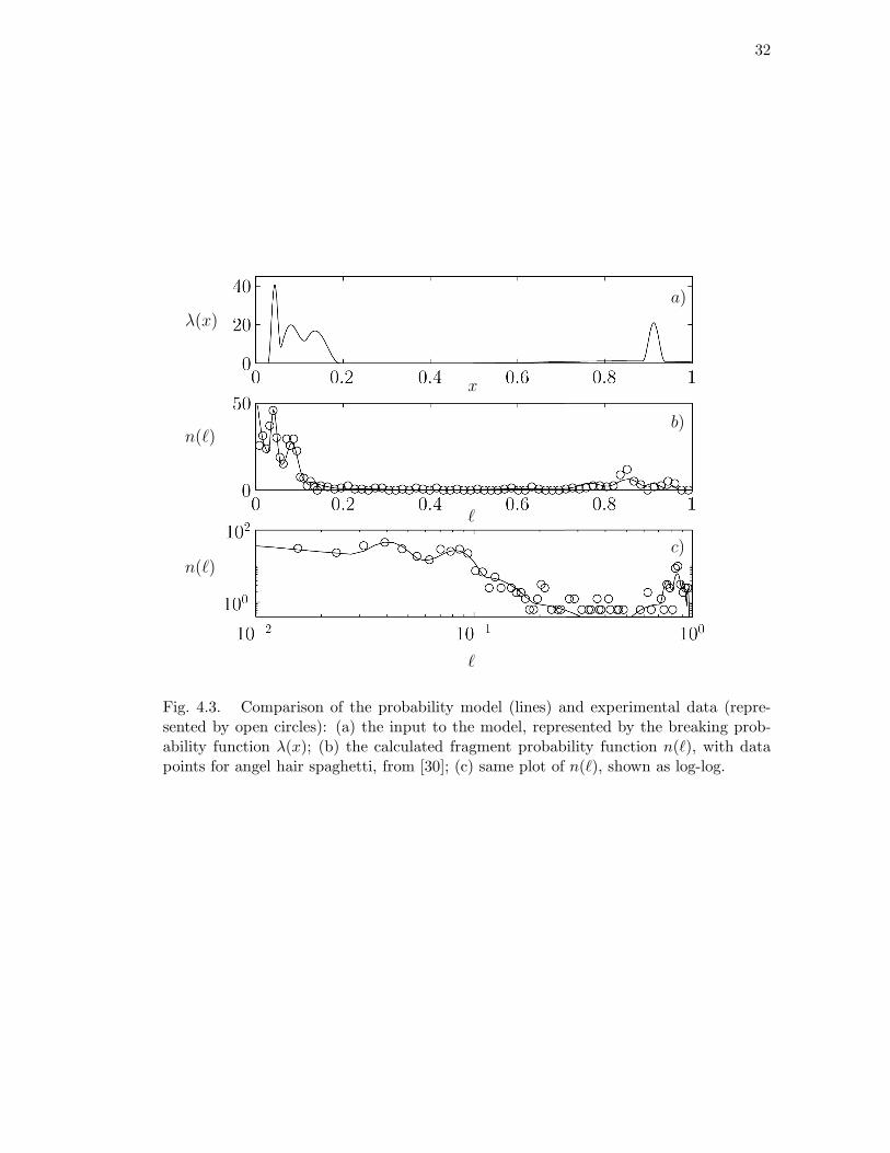
32
λ(x)
x
n(`)
`
n(`)
`
a)
b)
c)
Fig. 4.3. Comparison of the probability model (lines) and experimental data (repre-sented by open circles): (a) the input to the model, represented by the breaking prob-ability function λ(x); (b) the calculated fragment probability function n(`), with datapoints for angel hair spaghetti, from [30]; (c) same plot of n(`), shown as log-log.

33
m=1 2 3 4 5 6
Am (amplitude) 46.19 26.16 1095.20 9.77 1.76 30.77π/Bm (width) 0.06 0.07 0.07 0.24 0.75 0.03Cm (center) 0.05 0.11 0.22 0.37 0.60 0.87
Table 4.1. Fitted parameters for the pulses in Eq. 4.1, used for the curves shown inFig. 4.2
For both experimental data sets we see a similar general pattern in λ: severalpulses clustered near the impacted end (x = 0), with a low, wide pulse further down,and a narrow pulse near x = 0.9. The differences in the λ(x) shown for the differentexperiments confirm that it is not possible to determine the form λ(x) takes by merelyfitting parameters. To actually measure λ(x) we performed a new experiment in whichwe measured the positions of breaks as well as the sizes of fragments obtained.
4.2.2 Measuring λ(x) experimentally
In many of the fragmentation problems studied in engineering or geophysics, dataconsists of only the fragment distributions n(`). However, the experiments described in[30] allow in principle for the measurement of both the probability of breaking along the
rod and the resultant fragment distribution. Here we report a preliminary measurement †
of λ(x) for brittle rods in a similar experimental setup, from which we make a comparisonbetween the fragment distribution n(`) as calculated from Eq. 3.12 and the directlymeasured distribution.
The experiments were performed with spaghetti (San Giorgio angel hair) of lengthL = 17±0.1 cm diameter d ≈ 0.85 mm, kept upright by holding one end in an aluminumbase. A cylindrical brass weight of 51 g was dropped onto one end of the pasta, impactingwith a velocity of about 4 m/s; an example of the resulting fragmentation is shown inFig. 4.4. For our experimental parameters, the predicted buckling wavelength is 3.6 cm[30], while observation of the images indicate a wavelength of 3.2 cm (see Fig. 4.5b).
The experiments were filmed at 11,111 fps using a Phantom v5.0 high-speed digitalvideo camera. In each image the pasta is directly visible, as is a mirror image (seeFig. 4.4). The angle of the mirror was controlled so that on the line where the pasta satthe images were orthogonal. This was accomplished by sighting along pins set througha piece of graph paper into a block of wood that was milled flat. Only about 8 cm of thespaghetti is visible in all of the photos, so data collection was restricted to this range.The independence assumption of our model allows us to treat the breaks in this sectionof the rod as if it was the whole rod: we simply normalize our data to the length of thesection (8 cm) instead of by the total length L.
†A major limiting factor has been the frame size captured by our camera at higher framerates. Advances in new camera technology are already sufficient to allow for more detailedmeasurements. The Phantom V710 for example is advertised with a maximum frame rate of1, 400, 000 fps.

34
Fig. 4.4. Two simultaneous orthogonal perspectives of the fragmentation of a brittle rod(spaghetti) under the impact of a projectile moving at 4 m/s (see text). The dynamicbuckling of the rod before fragmentation leads to a pattern in the location of break, hereinto 8 fragments. The time from impact to fragmentation is less than 5 ms.
We used images of the pasta just after it broke to record the locations of breaksalong the length of the spaghetti. This provided us with experimental values of both λ(x)and n(`) (see Figures 4.5 and 4.7). Note that the measured n(`) is somewhat differentthan what would be measured by picking up the pieces afterwards - it does not includeany secondary breaks due to fragment collisions after the primary event (including thebrass re-impacting the unbroken end of the pasta, or curvature dynamics leading tofurther breaking [4]).
We compared the measured values of n(`) with values calculated from the exper-imental values of λ(x) to see if the relationship is well described by Eq. 3.12. Moreover,we expanded this comparison to all possible values for λ(x) that lie within the 95% con-fidence interval of the experimental values. Unfortunately, even the closest fit – shownin Figures 4.6 and 4.7 – has obvious differences with measured values of n(`). The differ-ences do not necessarily indicate that the hypotheses leading to Eq. 3.12 are incorrect:There are many sources of error, including low statistical numbers and limited opticalresolution. What is important is that the fragment distributions compared in Fig. 4.7come from the same set of measurements, and that - with the exception of an apparentexperimental peak at ` ' 0.3 - the features of the experimentally measured fragmentdistribution are qualitatively captured by Eq. 3.12.
4.3 Discussion and Conclusions
The mathematical framework developed here provides an explicit answer to theprimary hypothesis put forward to explain the non-power law distribution observed in

35
a)
b)
Fig. 4.5. Observed patterns in the probability of breaking: a) measured probabilityof breaking λ(x) over 175 events (see text); b) several cases of the initial buckling con-tributing to λ(x), where the buckling plane was almost entirely in a single plane of view.The error bars are produced by considering the measurements for λ(x) as independentexperiments for different values of x.

36
Fig. 4.6. The open points are the measured distribution for λ(x), while the solid pointsshow values within the 95% confidence interval of these measurements that provide abest approximation to measured values of n(`).
Fig. 4.7. Calculated and measured values of n(`) for the experiment described in Fig. 4.4.The open points are the measured distribution, and the solid points show the calculatedn based on values shown in Fig. 4.6. Note that the discretization of the calculated ncomes from the discrete measurements of λ(x).

37
[30]; it also goes much further, allowing us to map any 1D probability of breaking alongthe length of a rod to its resultant fragment distribution. Often in fragmentation studiesin engineering or geophysical applications, one does not have access to this originalprobability of breaking, usually because the fragmentation process itself was not observed- this is typically true for accidents, for which determining the cause of the failure, andtherefore the original stress distribution, is often an important goal. While the inverseproblem is evidently complicated, it can be done numerically, as we have shown inattempting to fit the data shown in Fig. 1.1. Note however that while the expectedtotal number of fragments is easily obtained in our framework, it remains to connect thisquantity to the energy input into the object, via impact or other mechanisms [33].
Our derivation relies on a generalization of the Poisson process, which underliesseveral complex and accepted models for fragment distributions [65, 3, 29]; however, itsutility for describing fragment distributions in one dimension is often dismissed [63, 1]since it is thought to produce only exponential fragment distributions. In modeling ourown one dimensional experiment, we have shown the fragment distributions producedby such a Poisson process to be much more rich and complex.

38
Chapter 5
A sphere sinking in bubbles: introduction
Visual perception is tuned to motion, indeed objects that are motionless on theretina, or even move slowly compared to other objects can be subject to ‘visual disap-pearance’ [12]. Little wonder then that motion of terrestrial and celestial bodies formsone of the oldest and most basic branches of physics. Modern treatment of the subjectis formalized with Newton’s (1642 - 1727) second law
the alteration of motion is ever proportional to the motive force impressed;and is made in the direction of the right line in which that force is impressed[69]
or, more familiarly the net force on a body F is related to its acceleration a by F = ma
or to its momentum P by F = dP/dt. With this simple formula, the motion of everydayobjects can be described. Experience teaches us, however, that the motion of objectscan be complex and unexpected. Indeed, the simple form of Newton’s second law beliesthe complexity of the assorted phenomena that can create these forces.
The simplest experiments observe motion under the influence of gravity using thesimplest of shapes - a sphere. One early and famous experiment was one attributed(posthumously by Vivandi) to Galileo (1564 - 1642) in which he dropped spheres ofdifferent weights from the leaning tower of Pisa to show that they fell at the same speedand not (as supposed from Aristotelean mechanics) in inverse proportion to their weights[17].∗ Contemporaries such as Simon Stevin (1548 - 1620) and Jan Cornet de Groot (1554- 1640) were performing similar experiments. Stevin, for example, records dropping twolead spheres from a height of thirty feet and observing that the sounds of their impactswere simultaneous [87].
Stevin also briefly describes two other factors that can be seen in the gravity-driven motion of experiments dropping spheres in air or water – buoyancy and resistancefrom the surrounding fluid [87]. The principle of buoyancy has been known, of course,from the time of Archimedes: there is an upward force on an object equal to the weightof the fluid it displaces. The effect of other forces on a sphere moving in a fluid, onthe other hand, is complicated by the need to know how the fluid is moving about thesphere.
∗Whether this experiment was actually performed has been questioned [18, 17]. Other ex-periments recorded during Galileo’s lifetime reported somewhat different results – a wooden andiron ball were released from a height. Initially the wooden ball was seen to lead the iron ball,which overtook it and struck faster. This appears to be a combination of air resistance slowingthe wooden ball to a greater extent, and muscle fatigue which causes the iron ball to be releasedmore slowly [18].

39
Our own experiments will follow the grand tradition of sphere dropping † by ob-serving the motion of a sphere settling in a bubbly fluid. The effect of bubbles on asinking sphere depends largely on the relative size of the sphere and bubbles. For exam-ple, the effect on a large sphere may be to reduce buoyancy by making the surroundingfluid less dense on the average, causing the sphere to sink more quickly or even to sinkwhen it may have been buoyant in quiescent water . The effect is exacerbated by abubble “shadow” above the sphere where the fluid is at its normal density.[22]
On the other hand, a small, hydrophobic particle can attach to a bubble and floatfree of a suspension. This process can be used, for example, in ink recycling. The paperis pulped and put into a dilute suspension where ink particles are separated chemicallyand mechanically from paper fibers. The suspension is also chemically treated to makeink particles more hydrophobic. After this, bubbles are run through the suspension,carrying ink particles to the top of the fluid where it is removed as a foam or scum (seee.g. [48]).
Our experiments will focus on a middle regime where the bubbles and the sphereare the same size. This interest was originally sparked by Professor Eduardo Ramos ofUNAM, with whom we have discussed the use of bubbles for suspending and mixingparticles. We are interested in spheres that do not necessarily fall or float in the fluid.We will in fact see a transition from floating to falling based on the size and massof the sphere and the flow rate of the rising bubbles. Our first experiment will focusmostly on the settling (terminal) velocity of the spheres. Aside from the effect of directinteractions between the bubbles and spheres, we will need to take some account of thefluid-sphere interaction. We devote the remainder of this introduction to a brief reviewof the equations governing fluid motion and its interaction with a sphere. We will returnto these in later chapters while modeling the motion of the spheres.
The motion of many fluids can be described by the incompressible Navier-Stokesequations (even for such fluids as air, which are compressible) where the fluid velocity u
is given by
ρ
[
∂u
∂t+ (u · ∇)u
]
= −∇p+ µ∆u (5.1)
with the incompressibility condition
∇ · u = 0. (5.2)
Here p is pressure, ρ the fluid density and µ the viscosity of the fluid (see e.g. [54]).
†The author also follows a more personal history of his grandfather Dee H. Barker’s disser-tation “The effect of shape and density on the free settling rates of particles at high Reynoldsnumbers”. This tradition is a little less grand, as Dr. Barker contracted arsenic poisoning (painfulbut fortunately not fatal) by dropping spheres down smoke-stacks.

40
The total force on a sphere of mass m comes from body forces such as gravityand from surface forces acting on the surface ∂S of the sphere. That is,
F = mg +
∫∫
∂STn dS (5.3)
where n is the outward unit normal vector to the sphere, and the components σij of thestress tensor T are related to Eq. 5.1 by
σij = −pδij + µ
(
∂ui
∂xj+
∂uj
∂xi
)
(5.4)
(see e.g. [54]).The forces on the sphere can be rewritten to highlight various effects of the fluid.
G. Mougin & J. Magnaudet [67] for instance, detail generalized equations – originallydue to Kirchoff – for the motion of a submerged rigid body of volume V. In the labinertial frame, the center of mass of the body has velocity U while the rotation rateof the body is Ω. The equations of motion are framed in body-centered coordinates(coordinates that center on the center of mass of the body and rotate at the rate Ω.)This allows the components of the inertia tensor, among others, to remain constant inthe equations. In these coordinates
(mI+ A)dU
dt+Ω× ((mI+ A)U) = Fω + (m− ρV)g (5.5)
and
(J+ D)dΩ
dt+Ω× ((J+ D)Ω) +U× (AΩ) = Γω. (5.6)
The quantities I, A, J, D are the identity tensor, added mass tensor, inertia tensor andadded inertia tensor. The quantities Fω and Γω represent force and moment about thecenter of mass due to vorticity in the fluid.[67]
The added mass and rotational inertia represent momentum and angular momen-tum in the fluid corresponding to the velocity and angular rotation of the body. Thesequantities are calculated as if the body moved in an unbounded ideal fluid.[67]
For a sphere the equations simplify considerably as A = 12ρVI, J = 2
5mr2I andD = 0. This allows us to rewrite Eq. 5.5 as
(
m+1
2ρV)(
dU
dt+Ω×U
)
= Fω + (m− ρV)g. (5.7)
Here the quantity dUdt +Ω ×U can be replaced by dU
dt by fixing the coordinate systemin the lab frame rather than allowing it to move and rotate with the sphere [24]. Thisleaves us with the equation of motion
(
m+1
2ρV)
dU
dt= (m− ρV)g + Fω. (5.8)

41
Some examples of approximations to Eq. 5.1 which follow the form of Eq. 5.8 (seee.g. an overview in [49]) are those derived by Basset, Boussinesq and Oseen for creepingflow ( i.e. where ∇p = µ∆u )
(
m+1
2ρV)
dU
dt= (m− ρV)g − 6πaµU− 6a2
√πµρ
∫ t
0
dU/dτ√t− τ
dτ (5.9)
and by Maxey and Riley for unsteady creeping flow [49]
(
m+1
2ρV)
dU
dt= (m− ρV)g + 6πaµ(u−U) +
3
2ρV du
dt
+1
2ρV(u · ∇)u+ 6a2
√πµρ
∫ t
0
d(u−U)/dτ√t− τ
dτ
(5.10)
The latter equation has been adapted (Berlemont, Desjoonqueres and Gouesbet [49]) toapproximate the effect of more general flows as
(
m+1
2ρV)
dU
dt= (m− ρV)g +
1
2πa2ρCD|u−U|(u−U) +
3
2ρV du
dt
+1
2ρV(u · ∇)u+ 6a2
√πµρ
∫ t
0
d(u−U)/dτ√t− τ
dτ
(5.11)
using the form drag approximation 12πa
2ρCD|u−U|(u−U) that will be described laterin this section.
In 1851, G. G. Stokes established one case in which solutions for the effect of afluid on a sphere of radius a can be calculated. He examined the case of a sphere insteady translational motion U in a unbounded fluid in which the inertia terms on theright hand side of Eq. 5.1 are negligible. In this case the simplified equation is
∇p = µ∆u. (5.12)
Additional condition are that u→ 0, p→ p0 as |x| → ∞, and on the surface of the sphereu = U (impermeability and no-slip boundary conditions). In this case the movement ofthe fluid is symmetric about the axis along which the sphere moves. In polar coordinateswith θ = 0 in the direction of U, the components of velocity are taken from the streamfunction
Ψ = Ur2 sin2 θ
(
3
4
a
r− 1
4
a3
r3
)
(5.13)
with
ur =1
r2 sin θ
∂Ψ
∂θ= U cos θ
(
1− 3R
2r+
R3
2r3
)
(5.14)
and
uθ = −1
r sin θ
∂Ψ
∂r= U sin θ
(
−1 + 3R
4r+
R3
4r3
)
(5.15)

42
(see e.g. [10, 54, 71]).By symmetry, any force must be directed parallel to the line of motion. On the
surface of the sphere, this component of force is given [54] from Eq. 5.4 by
F =
∫∫
r=a−p0 cos θ +
3µ
2aU cos2 θ +
3µ
2aU sin2 θ dS = 6πµaU. (5.16)
It is also possible to calculate the drag on a sphere in steady motion in circum-stances where the inertial terms of Eq. 5.1 are important, but the dissipative term µ∆u
is negligible. In the case of an unbounded ideal fluid (µ = 0) in irrotational motion, theflow around a sphere of radius a rising at a speed of U is given by
u = −1
2Ua3∇ z
(
x2 + y2 + z2)3/2
(5.17)
where the center of the sphere is located at the origin [10]. Because the fluid flow andsphere surface are symmetric before and behind the sphere, the net force from Eq. 5.4must be 0, giving an example of d’Alembert’s paradox that there is no drag on a bodyin steady motion through an ideal fluid [16].
In most circumstances however, one is not able to analytically determine the effectof the fluid on a submerged sphere and must rely on either numerical or ad-hoc methods.One rule of thumb usable at higher Reynolds numbers – where the flow separates fromaround the back of the sphere – is the concept of form drag. The idea is that the fluidupstream moving relative to the body at speed U stagnates at the surface over a shortdistance. From Bernoulli’s equation [54]
1
2u2+
p
ρ+ gz = constant (5.18)
we see that (since ∆z ≈ 0 as the fluid decelerates)
∆p ≈ −ρ
2∆u
2 =ρ
2U2. (5.19)
With a forward facing surface with projected area A = πr2, this pressure differencecreates a force of
F ≈ ρπr2
2U2 (5.20)
downstream (i.e. opposing the motion of the sphere). There is not a correspondingpressure change behind the object where the fluid inside the separated streamlines movesat about the same velocity as the sphere [10]. However, because not all the streamlinesin the area in front of the sphere stagnate at the surface Eq. 5.20 is at best an argumentfor the order of magnitude of the drag, and one looks for a drag coefficient CD so that
F =ρCDπr
2
2U2 (5.21)

43
[10]. The drag coefficient on a sphere has been measured by many experiments and
compiled as a function of Reynolds number (Re = ρdsUµ ) into the standard drag curve
[16] shown in Fig. 5.1.
100
101
102
103
104
105
106
10−2
10−1
100
101
102
CD
Re
Fig. 5.1. The standard drag curve from [16] gives the coefficient of drag for Eq. 5.21 asa function of a sphere’s Reynolds number.
In the following chapters we will present an experiment of a sphere settling in abubbly fluid. We will show that in our experimental setup, the settling velocity of thespheres in the bubbly fluid is dominated by the form drag of Eq. 5.21. We will afterwardsexamine the effect of collisions between bubbles and the settling sphere seeing how thisaffects not only the settling velocity, but the lateral dispersion of spheres falling in abubbly fluid.

44
Chapter 6
A sphere sinking in bubbles: settling velocity
6.1 Experimental setup
6.1.1 The container
To observe the motion of a sphere sinking in a bubbly fluid, we constructed aquasi-2D experiment in which the bubbles and the sphere were confined to a narrowchannel with inner dimensions of 2 cm × 18.4 cm × 30.6 cm (see Fig. 6.1). This acryliccell was supported by four stainless steel bolts used to raise lower and level the cell.Performing the experiment in a narrow cell had two significant advantages. First, wehad found that in a more fully 3D experiment (as seen in Fig. 6.2) the spheres (eventhe largest we used) were hard to observe. Secondly, we wished to capture as much ofthe motion as possible when we recorded the experiment. The cell was placed in an 18gallon tank which was filled with tap water. Bubbles were generated below the cell, whilespheres were released slight inside the top of the cell (or in some cases at the bottom.)The experiment was lit from behind using halogen lights with a translucent plastic sheetacting as diffuser, and the progress of the sphere through the cell was captured on video.
6.1.2 The bubble field
The bubbles in this experiment were produced by an Aquatic Gardens BubbleBar, an “air stone” commercially available for aquariums. The bar was centered underthe cell and held in place with brass weights during the experiments. Air to the stonecame from the building’s compressed air source through a valve monitored by an Omega1200 series digital pressure gauge. To prevent bubbles from coalescing on the undersideof the cell and rising inside the cell, the walls at the bottom were tapered to direct suchbubbles towards the outside of the cell.
To measure the properties of the bubble field, we first measured the gas flow rateas a function of the applied overpressure (gas pressure above the ambient air pressurein the lab). Bubbles were funneled from 9.5 cm of the air-stone into an upside-downbeaker. The amount of air in the funnel was constant, so the inflow and outflow werethe same. The collection time and volume of the collected gas were measured to findthe volume flux per centimeter along the stone. The results are shown in Fig 6.3. Asa function of applied overpressure pa [psi], the flux per centimeter, f is approximately
f = (1.0pa[psi]− 1.5) cm2/s.Next we measured the number density of bubbles per unit volume. We counted
for several pressures the number of bubbles in sections of images 184pixels×196pixels.Because bubbles coalesce as they rise, the number density near the bottom of the tankis higher than that near the top of the tank. Results are shown in Fig. 6.4. The average

45
Fig. 6.1. The first experimental setup for observing a sphere settling in a bubbly fluid.Fabrication was by R. Geist of the Pritchard Lab. See text for details.

46
Fig. 6.2. A fully 3D bubble field produced by an array of commercial air stones.

47
2 3 4 5 6 7 80
1
2
3
4
5
6
7
f [cm2/s]
pa [psi]
Fig. 6.3. Bubble volume flux per centimeter f [cm2/s] as a function of applied overpres-
sure pa [psi]. The dashed line shows the approximation f = (1.0pa[psi]− 1.5) cm2/s.
number of bubbles per cubic centimeter is approximately N = (0.098pa[psi] + 2.9) cm−3.
Finally, we measured the rise velocity of the bubbles as a function of the appliedoverpressure. This was done by picking bubbles that appeared to be moving at theaverage speed of the bubble field and recording their rise times over as long a distanceas possible. These results are shown in Fig. 6.5. We find that the average rise velocityis approximately Ub ' (3.5pa[psi] + 37) cm/s.
From these measured quantities, we can derive the void fraction: In one secondthe air released from one centimeter’s length of the stone rises Ub cm into a channelof 2 cm width. Thus in 2Ub cm3 of water we have f cm3 of air for a void fraction off/ [2Ub], which averages to 3.2% in the range of pressures shown. We can also calculatethe average volume equivalent diameter de of the bubbles. That is, as the bubbles areellipsoidal rather than spherical, we use the diameter of a sphere of equivalent volume.In our case we will calculate the volume of a bubble based on the volume of air in a cubiccentimeter f/ [2Ub] divided by the number of bubbles per cubic centimeter N , giving us
de =f
2Ub ·N(6.1)
the results of which are shown in Fig. 6.6. The average of the values shown from3 ≤ pa ≤ 7 psi is de = 0.26 cm.
These measurements of the diameter are similar to visual measurements made ofellipsoidal bubbles produced by the air-stones in Fig. 6.2. The major and minor axis(dM and dm) of 45 bubbles were measured, the sample evenly distributed among higher

48
3 3.5 4 4.5 5 5.5 6 6.5 70
1
2
3
4
5
6
7
N [cm−3]
pa [psi]
Fig. 6.4. Bubble number density N [cm−3] as a function of applied overpressure pa [psi].Measurements shown in blue indicate values in the lower part of the cell. Measurementsin red show values in the upper part of the cell. The dashed lines approximate their valuesas N = (0.049pa[psi] + 3.5) cm−3 and N = (0.15pa[psi] + 2.2) cm−3 respectively. Theblack line shows the average for the cell approximated as N = (0.098pa[psi] + 2.9) cm−3.
2.5 3 3.5 4 4.5 5 5.5 6 6.5 7 7.540
45
50
55
60
65
70
Ub [cm/s]
pa [psi]
Fig. 6.5. Bubble rise velocity Ub [cm/s] as a function of applied overpressure pa [psi].

49
3 3.5 4 4.5 5 5.5 6 6.5 70.2
0.22
0.24
0.26
0.28
0.3
0.32
de [cm]
pa [psi]
Fig. 6.6. Plot of equation 6.1: bubble volume equivalent diameter de [cm] as a functionof applied overpressure pa [psi].
and lower bubbles. We then calculated de = 3
√
d2Mdm . The average diameter in this
case was found to be de = 0.2 cm.Some of the average bubble properties are listed in Table 6.1. These include
the bubble Reynolds number (Re = ρUbdeµ – used to characterize flow in the non-
dimensionalized Navier-Stokes equations) and the Eotvos number (Eo = |g|∆ρd2e/σ
where σ is the surface tension of the air-water interface, which we take to be 72 dyne/cm.)The Reynolds number and Eotvos number can be used, for example, to characterize theshapes of bubbles (e.g. spherical, ellipsoidal, wobbly, spherical cap, etc.) as in [16]. Inour case, the numbers indicate bubbles that are ellipsoidal with a tendency to becomewobbly as they rise. This seems to match experimental observations of both ellipsoidalbubbles and bubbles that flattened and changed in shape as they rose.
6.1.3 The spheres
Apart from the applied overpressure, the controllable variables in the experimentwere the size and density of the spheres being dropped (since the cell geometry, bubblegenerator and fluid were not changed during the course of the experiment). Two mainmaterials, glass and Teflon, were used in a variety of sizes from about a half a centimeterto a centimeter. One series of a fixed diameter was also tested for a number of othermaterials as shown in Table 6.2.
The spheres were initially inserted into the bubble field by hand, but we discoveredthat the presence of fingers in the stream noticeably altered our results. For example, asphere dropped in quiescent water would often move obliquely to the side in its descent,

50
Property Average Value
f (gas flow rate) 3.5 cm2/s
N (number density) 3.4 cm−3
Ub (rise velocity) 54 cm/sde (volume-equivalent diameter) 0.26 cmvoid fraction 3.2 %Re (Reynolds number) 620Eo (Eotvos number) 0.92
Table 6.1. Average properties of the bubble field for 3 ≤ pa ≤ 7 [psi].
Material Diameter (cm) Density (g/cm3)
Black Glass 0.48, 0.64, 0.79, 0.95 2.61
Delrin 0.79 1.35
Lucite 0.79 1.19
Nylon 0.79 1.14
Teflon 0.48, 0.64, 0.79, 0.95 2.17
Viton 0.79 1.8
Table 6.2. Properties of the spheres used in the first experiment.
even though its initial movement was downward. As the wakes of spheres are knownto produce lift (see e.g. [43]), we speculate that the presence and movement of ourfingers created an asymmetry in the developing wake of the spheres.∗ After this, theexperiments were repeated using tweezers to place the spheres into the tank. Care wastaken to make sure that the spheres were thoroughly wetted and free from any attachedbubbles before being inserted into the stream. Spheres light enough to rise in the streamwere released at the bottom of the cell rather than near the top.
6.1.4 Extracting data
Experiments were recorded using the lab’s Phantom V5 high-speed digital videocamera. A typical video had a frame size of 1024pixels×1024pixels, recorded at 300fps. The videos were cut at the time of recording so that the sphere was present inimage. The videos were transferred from a proprietary format to AVI files for analysis.An application for extracting location data from the AVI files using was created inMicrosoft’s C# because of useful and publicly available libraries for reading and writingto AVI files.
∗There is a parallel used in experiments observing the wake-induced zigzag motion of bubbles:the plane of the zigzagging motion can be controlled by producing the bubbles using an angledhypodermic needle. The (vertical) plane of the zigzagging motion is perpendicular to the angledface of the needle (see e.g. [85]).

51
The process of algorithmically locating the sphere within the images contained inthe AVI files evolved over time. For the data presented in the first experiment, the sizeof the sphere and its location for one frame in the image were set by the user, along witha maximum search width. Beginning at the known location, the program would advancea frame and check the pixels in a box extending a distance of the search width from thelast known location. The pixel with the darkest set of pixels within a sphere radius wasdetermined to be the center of the sphere, and the process was repeated for the wholesequence of images.
After processing, the video was played back with the position and path of thesphere superimposed. It did happen at times that, because the sphere was often obscuredfor a short time, a bubble might be identified and tracked as the sphere. In cases wherethis happened, the location was manually adjusted, and the video re-analyzed from thatpoint. A picture of a sphere in the bubble field shown in Fig. 6.7 gives some indicationof the difficulty of the process. A path showing a sphere trajectory over the course of anexperiment is shown in Fig. 6.8.
The location data were analyzed over about 15 cm of the height of the cell. Thiswas done to give the sphere time to accelerate, and to avoid the turbulent region near thebottom of the cell where the flow and sphere behavior were noticeable different. (Lighterspheres would often be trapped for a short time in this region.) The average velocity
over the measured distance was taken to be the terminal velocity of the sphere.†
For later experiments we became interested in having more detailed informationabout a sphere’s position and progress through the tank. We therefore adjusted thelocation algorithm as follows: first a mask was made by making a scale measurement(px/cm) in an image, and entering the known diameter of the sphere. A mask was madeusing the sphere diameter with a Gaussian drop in intensity from interior to exteriorpixels. The actual foreground and background brightness values were left variable, asthere is sometimes a change in the lighting intensity.
A foreground and background brightness for the mask were chosen by looking forthe brightest and darkest pixels in the search area. The pixel location of the sphere wasdetermined as before by looking for the minimum error between the masked and actualbrightness values. This constituted a rough search and gave a preliminary position forthe location of the center.
To better determine the center of the sphere, we used the following algorithm.The rough location of the center was at (i, j). We define the function b(m,n) to be thebrightness value at pixel (m,n). Let ∆x = x− bxc and ∆z = z − bzc (where bzc is the
†The averaging scheme for measuring terminal velocities was adopted because of fluctuationsin the measured velocity of the spheres over smaller time scales. The largest, heaviest spherestake longer to reach their terminal velocities, and the averaging method may underestimate thosenumbers.This showed a need to be able to more accurately measure sphere positions and velocities.
Some of the fluctuations in speed were because of sphere-bubble interactions, but some camefrom limited resolution of the sphere locations. This was part of the motivation for the moreaccurate location algorithms developed to track spheres in later experiments.

52
Fig. 6.7. Images from an experimental video. In this image the sphere (silicon nitrided = 3/32”) is indicated by a red arrow.

53
Fig. 6.8. Image from an experimental video. In this image the sphere (silicon nitrided = 3/32”) is highlighted in red, and its path to that point is shown in yellow.

54
greatest integer less than or equal to z). We further define
B(m,n, x, z) = (1−∆x)(1−∆y) b(m− bxc, bn− bzc)+∆x(1−∆y) b(1 +m− bxc, bn− bzc)+∆y(1−∆x) b(m− bxc, 1 + bn− bzc)+∆x∆y b(1 +m− bxc, 1 + bn− bzc)
(6.2)
that is, as if a square representing one pixel were shifted to cover adjacent pixels also,and the brightnesses summed proportionally to the area covered.
The quantity B(m,n, x, z) was now compared to the brightness values in themask, and the difference measured. To minimize the error, we implemented a steepestdescent line search, with the step lengths chosen to satisfy the Strong Wolfe Conditionsusing algorithms from [70]. To observe the effect of the sub-pixel location algorithm,we chose videos of spheres in quiescent water (where the motion is naturally smootherthan in the bubbly fluid). Videos extracted from the larger image and centered on theinteger pixel location were compared with videos extracted using the sub-pixel locationand averaging schemes. The sub-pixel algorithm provided a noticeable stabilization ofthe sphere at the center of the images.
6.2 Findings: terminal velocity in quiescent and bubbly water
For a sphere settling downward at a terminal velocity Vt the form drag of Eq. 5.21balances with buoyancy to give
4
3πr3
s(ρs − ρ)|g| = 1
2CDρV
2tπr2
s(6.3)
so that
Vt =
√
8rs(ρs − ρ)|g|3CDρ
∝√
rs(ρs − ρ)|g|ρ
. (6.4)
Measured velocities of Vt are shown in Fig. 6.9. The square-root dependence is alsoshown, best fit by CD = 0.56 — a value comparable to that expected without the cell.
For convenience, we will refer to the quantity determining form drag rs(ρs−ρ)|g|ρ from
Eq. 6.4 as
∆fd ≡rs(ρs − ρ)|g|
ρ.
In Fig. 6.10 are shown measurements of the terminal velocities of spheres both inquiescent water and in bubble fields at a variety of applied overpressures. Note that thedownward velocity is no longer as steady in these cases, and represents an average settlingspeed. One major effect of the bubbles is to decrease the terminal velocity of the spheres.In fact, there is a distinct transition where the spheres move from sinking to rising in thewater. A picture of this transitional behavior is shown in Fig. 6.11. In addition to theslowing of the spheres’ terminal velocities we also see that the in the bubbly fluid thereis some random lateral motion. Although our motivation in performing this experiment

55
200 300 400 500 600 700 80035
40
45
50
55
60
Vt (cm/s)
∆fd (cm2/s2)
Fig. 6.9. Measured values of the terminal velocities of spheres in quiescent water. Thedotted line shows the square-root dependence of Eq. 6.4 with CD = 0.56.
was to control the settling speed of the spheres in order to suspend them, this secondeffect is of interest and will be considered later in this work.
6.3 Observations: bubble-sphere interactions
There are at least three types of interactions we observed between the bubblesand the spheres. The first is that bubbles can attach to spheres. We found this tohappen most often when using Viton or one of the plastics. Depending on the numberof bubbles attached to the spheres, the sphere was slowed in its descent or even floated.This is visible in Fig. 6.12 where the sphere on the left has one attached bubble, and anidentical sphere on the right has three bubbles attached to it.
The second interaction is the entrapment of air bubbles in the wake of a sphere.We show two typical examples. In Fig. 6.13 a bubble is trapped in the wake of a smallersphere (d = 0.48 cm). It stays at a fixed distance from the sphere for a short time,until another bubble collides with it and carries it away. In Fig. 6.14 a larger sphere(d = 1.27 cm) captures many bubbles in its wake. These bubbles can be seen being shedin groups during the earlier stages of the sphere’s acceleration.
The third interaction is the collision of spheres and bubbles. These are most ofteninferred by us rather than observed: In a video recorded at, say, 100 fps a bubble willtravel about a sphere diameter every frame, making collisions hard to observe. We have,however, isolated images of a collision which can be seen in Fig. 6.15.

56
0 100 200 300 400 500 600 700 800−20
−10
0
10
20
30
40
50
60
70
Vt (cm/s)
∆fd (cm2/s2)
↑ Sinking
↓ Rising
Fig. 6.10. Measured values of the terminal velocities of spheres in quiescent water (blackcircles) and in bubbles (blue circles) at a variety of pressures.
6.4 Bubble-flow interactions
Aside from the bubble-sphere interactions, there is one more factor to be con-sidered. Because the cell is open at the top and the bottom, bubbles rising in the cellentrain water and cause a net flow of water up through the cell. By measuring the risetime of buoyancy-neutral particles ‡ (see Fig 6.16), we discovered that water circulatesup through the cell at a velocity of Uw = (3.4pa[psi] + 13) [cm/s]. Note that in this case,the return flow is outside the cell, a major difference from a closed geometry such as thatin [100] where the net circulation of water through the cell is zero.
The difference of 24 cm/s between the circulation velocity and bubble velocityis about the speed of a single similarly-sized bubble in quiescent water [16]. Becausethe bubble velocities are consistent across the width of cell, we infer that the circulationvelocity is also uniform (except of course at the very edge of the cell). The observed rela-tion between the bubble velocity and circulation is supported by experiments comparingbubbly flow in a closed geometry with flow in which circulation was introduced [68]. Itwas discovered that difference between the bubbly flows with and without circulationwas approximately the circulation rate.
Because the water is circulating through the cell, it is appropriate to measuredrag on the spheres (and hence their terminal velocities) in the rest frame of the circu-lation. We see in Fig. 6.17 that by adjusting the terminal velocities of the spheres by
‡After several attempts to construct a buoyancy-neutral sphere, we decided to use smallclumps of towel lint which was observed floating at a constant depths in the tank.

57
Fig. 6.11. Left to right: spheres of glass, Teflon, Delrin, and Nylon (with diameters of0.79 cm). The last three spheres are in bubble fields at pa = 4 [psi].

58
Fig. 6.12. Two identical spheres are shown in successive images. In each image thesphere on the left has one bubble attached, while the sphere on the right has two. Theleft sphere is seen to be falling, while the right sphere floats.
the appropriate circulation velocity, that the difference between the terminal velocities inquiescent and bubbly fluids is almost entirely explained. Hence, if Vt is terminal velocityin quiescent fluid, the sphere is suspended between falling and floating when
pa[psi] ≈Vt − 13
3.4. (6.5)
If the relation of the rising bubbles to applied overpressure is unknown, it should alsosuffice to adjust the field until Ub −Vt is the same as the speed of a single bubble risingin quiescent water.
Although this satisfactorily answers the question of how to suspend a sphere (atleast in this experimental setup), it is very dependent on the geometry of the setup.It also fails to address the nature of the bubble-sphere interactions that were observed.Of the three described bubble-sphere interactions, we chose to focus on the effect ofcollisions. The next chapters will detail a model for the effect of collisions on the sphere,and a refined experiment used to observe these collisions and their effects.

59
Fig. 6.13. A bubble (colored for visibility) is trapped in the wake of a sphere (Teflon,d = 0.48 cm, ∆t = 5 ms).

60
Fig. 6.14. Bubbles are trapped in the wake of a sphere (glass, d = 1.27 cm, elapsedtime 107 ms) and periodically released in clusters. The cluster about to be released inthe second frame, for example, can be seen slightly above and to the right of the spherein the third frame. The group forming in the third frame can be seen in the fourth frameat a distance of about a sphere diameter above the sphere.
Fig. 6.15. A bubble(colored for visibility) collides with a sphere.

61
2.5 3 3.5 4 4.5 5 5.5 6 6.5 7 7.510
20
30
40
50
60
70
pa [psi]
Fig. 6.16. Bubble rise velocity Ub (in red) and water circulation velocity Uw (in blue)as a function of applied overpressure pa [psi].
0 100 200 300 400 500 600 700 800−20
−10
0
10
20
30
40
50
60
70
Vt + Uw
∆fd (cm2/s2)
Fig. 6.17. Measured values of the terminal velocities of spheres in quiescent water (blackcircles) and in bubbles (blue circles) in the rest frame of water circulating in the tank.

62
Chapter 7
A sphere sinking in bubbles: collision model
7.1 Introduction
Observing the erratic motion of the spheres in the experiments of the precedingchapter reminded the author of a game that used to sit in his grandparents’ basement –a “pachinko” machine brought back from their travels in east Asia (see Fig. 7.1). Thegame is intended for gambling: Small metal balls are purchased and inserted in theblue-and-white tray near the middle of the machine. They are then launched through atrack circling the left of the machine by use of the lever seen at the bottom right of themachine. The balls are released into free-fall near the top of the machine and bounceunpredictably among the pins as they fall. This erratic, collision-driven motion bearssome similarity to the motion of the falling spheres (particularly the smaller spheres)during repeated collisions with bubbles.
Fig. 7.1. The Barker family pachinko machine (photos by DeeAnne Higley). A payoffin the game comes when a ball enters one of the receptacles shown in detail to the right.
63
The mechanics of the pachinko machine are also reminiscent of the Galton boardor quincunx shown in Fig. 7.2. In this chapter we will examine the Galton board and itsmathematics as presented by various authors. We will then discuss a modification of theGalton board to represent the bubbly fluid discussed in the previous chapter. Finallywe will discuss a computer simulation of the fluid Galton model and highlight some ofthe results.
7.2 The Galton board
The Galton board described in Galton’s 1889 work Natural Inheritance consistedof a wooden back and a glass front “about a quarter of an inch” apart. Pins were fixed inthe board in quincunx fashion (that is, like the five spots on a dice, forming a triangularor hexagonal lattice). Small pellets poured into the top were funneled to the central partof the board where they fell among the pegs
scamper[ing] deviously down through the pins in a curious and interestingway; each of them darting a step to the right or left, as the case may be,every time it [struck] a pin. [28]
The pellets were collected at the bottom of the device in compartments. The height ofthe collected pellets was found to be consistent over multiple experiments and to closelyapproximate the normal distribution. The experiment was repeated by turning the frame“topsy-turvey”, with the pellets being collected by the inverse funnel at the top of theframe in position for another experiment.
Galton’s explanation for the distribution of the pellets is that as each drops fromrow to row it strikes a pin and is randomly shunted to the left or the right of it, inde-pendently of the history of its path. That is, in his own words,
the principle on which the action of the apparatus depends is, that a numberof small and independent accidents befall each shot in its career. In rarecases, a long run of luck continues to favour the course of a particular shottowards either outside place, but in the large majority of instances the numberof accidents that cause Deviation to the right, balance in a greater or lessdegree those that cause Deviation to the left. Therefore most of the shot findsits way into the compartments that are situated near to a perpendicular linedrawn from the outlet of the funnel, and the Frequency with which shotsstray to different distances to the right or left of that line diminishes in amuch faster ratio than those distances increase.[28]
We can be more precise about this process, as the mathematics of Galton’s expla-nation are straightforward. We will number the rows and columns of the lattice (i, j),beginning at the top row with i = 0 and with the column directly under the funneldesignated as j = 0. For example, the path of a pellet will always begin at (0, 0). Uponreaching the pin at (1, 0), a falling pellet – hereafter referred to as the tracer – is forcedinto one of the positions (1,−1), (1, 1). It is assumed that these outcomes are equallylikely. More generally, a tracer at position (i, j) is forced by the next pin into one of

64
Fig. 7.2. Galton’s board, the quincunx, as he portrayed it [28].
positions (i + 1, j − 1) or (i + 1, j + 1). Either of these events is assumed to be equallylikely, and thus independent of the history of tracer’s position.
The map from j → j + 1 has several consequences. As the tracer moves fromrow to row, the maximum allowable position of the tracer grows linearly, being i in theith row. Also, a tracer in an even(odd) numbered row can only occupy an even(odd)
numbered column. The allowable positions of the tracer in the ith row are then(i,−i), (i,−i + 1), . . . , (i, i).
There are 2i possible paths from (0, 0) into the ith row, each being equally likely.
The number of paths leading to (i,−i + 2j) is(
ij
)
, for 0 ≤ j ≤ i. Then the probability
that a sphere released at (0, 0) will be found at (i,−i+ 2j) is 2−i(ij
)
. This is a binomial
distribution, which for large values of i closely follows the normal distribution claimedby Galton (see e.g. [26]). A diagram of a few of these probabilities is shown in Fig. 7.3.
Due to the symmetry of the board, the expected value of j on the ith row is0 (even in odd rows where (i, 0) is occupied by a pin). The variance of the binomialdistribution is σ2 = 1
4 i, so that the variance in positions is σ2 = i (see e.g. [26]). Thelateral motion of the tracer is the familiar random (drunkard’s) walk. One importantaspect of the lateral motion is that if we assume that the tracer descends from row torow at a constant rate, then i = αt and σ2 = αt. The linear growth of the variance overtime is the hallmark of diffusive motion (see e.g. [23]). Hence if we model the movementof tracers through the board using Galton’s explanation, we can characterize the motionof the tracers as falling vertically and diffusing horizontally.

65
· 0 · 1 · 0 ·0 · 1
2 · 12 · 0
· 14 · 1
2 · 14 ·
18 · 3
8 · 38 · 1
8
Fig. 7.3. Probabilities that a tracer will reach given coordinates on the Galton board.
7.3 Examinations and adaptations of the Galton board
In this section we will discuss some recent investigations into the Galton boardand similar systems. In subsection 7.3.1 we will discuss treatments using experimentsand simulations, most often with statistical analysis or results in mind. In subsection7.3.2 we will review some treatment of the Galton board as a dynamical system. Thiswill preface section 7.4 in which we will make our own adaptation of the Galton boardfor modeling sphere-bubble collisions in a fluid.
7.3.1 Deterministic randomness
We begin by discussing an investigation motivated by interparticle percolation[62]. In a material containing mixed smaller and larger particles, the smaller can movedown through the larger when the material is under stress. Experimentally, Masliyahand Bridgewater used a bed of packed spheres into which smaller spheres were dropped[62]. If the ratio of sphere diameters is less than 0.1547, then the smaller spheres willsettle among the larger without becoming trapped. They found that the smaller spheressettled among the larger with the time of passage through the bed being proportional tothe height of the bed, i.e., with a constant average speed. Radially, the particles movedout diffusively from the center.
To be able to investigate the effect of physical parameters such as the intersticebetween the scatterers (packed spheres) they created a computer simulation. In thissimulation, the tracer moves from scatterer to scatterer under the influence of gravitywith the effects of air resistance neglected, that is, in parabolic paths with
δ2
δt2(x, z) = (0,−|g|) .
When the tracer reaches the surface of a scatterer, the interaction is modeled as aninstantaneous collision using the coefficient of restitution (see Appendix A for details).That is if vI is the incoming velocity and vR is the rebound velocity,
vR · n = −evI · n
where n is the unit normal to the spheres at the point of contact and e is the coefficientof restitution.
We wish to note here that one complication of the instantaneous collision modelis that it is possible for a large (or indeed, infinite) number of collisions to occur between
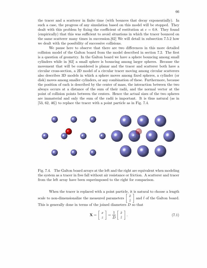
66
the tracer and a scatterer in finite time (with bounces that decay exponentially). Insuch a case, the progress of any simulation based on this model will be stopped. Theydealt with this problem by fixing the coefficient of restitution at e = 0.8. They found(empirically) that this was sufficient to avoid situations in which the tracer bounced onthe same scatterer many times in succession.[62] We will detail in subsection 7.5.2 howwe dealt with the possibility of successive collisions.
We pause here to observe that there are two differences in this more detailedcollision model of the Galton board from the model described in section 7.2. The firstis a question of geometry. In the Galton board we have a sphere bouncing among smallcylinders while in [62] a small sphere is bouncing among larger spheres. Because themovement that will be considered is planar and the tracer and scatterer both have acircular cross-section, a 2D model of a circular tracer moving among circular scatterersalso describes 3D models in which a sphere moves among fixed spheres, a cylinder (ordisk) moves among smaller cylinders, or any combination of these. Furthermore, becausethe position of each is described by the center of mass, the interaction between the twoalways occurs at a distance of the sum of their radii, and the normal vector at thepoint of collision points between the centers. Hence the actual sizes of the two spheresare immaterial and only the sum of the radii is important. It is thus natural (as in[53, 62, 46]) to replace the tracer with a point particle as in Fig. 7.4.
Fig. 7.4. The Galton board arrays at the left and the right are equivalent when modelingthe system as a tracer in free fall without air resistance or friction. A scatterer and tracerfrom the left array have been superimposed to the right for comparison.
When the tracer is replaced with a point particle, it is natural to choose a length
scale to non-dimensionalize the measured parameters
[
xz
]
and t of the Galton board.
This is generally done in terms of the joined diameters D so that
X =
[
xz
]
=1
D
[
xz
]
. (7.1)

67
The time is normalized by the free-fall time through a scatterer diameter so that
t = t/√
2D/|g|. (7.2)
The equation of motion in free fall then becomes
X =
[
0−2
]
. (7.3)
This also reduces the variable parameters of the Galton board model to two: the intersticefrom scatterer to scatterer and the coefficient of restitution. We note that in the studyof [62], the distance was normalized by the distance between scatterer centers. This leftthe free distance parameter to be the diameter of the scatterer.
The second and more troubling difference between the collision model of [62] andthe random walk model of [28] is that the motion of the tracer in the collision modelis fully specified: parabolic paths between collisions with a rebound law based on thecoefficient of restitution. The argument for diffusive behavior is no longer evident whensuccessive bounces no longer constitute a random walk. The system may now be treatedas a dynamical system for purposes of analysis, and indeed we will discuss at a laterpoint some results that may be obtained this way.
Masliyah and Bridgewater [62] make a case for treating successive jumps as iftheir lateral components were random (for purposes of analysis, not simulation). Thiscreates an effective random walk, explaining the diffusive behavior. We will follow theirarguments here. To analyze the path of a particle and decide whether its motions wererandom, they defined the net displacement of the tracer after n jumps as Rn =
∑ni=1
ri
where ri is the displacement from the ith jump. They also let r = limn→∞Rn/n anddefined the local fluctuations si = ri − r and the mean fluctuationSn =
∑ni=1 si = Rn − nr.
They calculated the magnitude squared of the mean fluctuation to be
|Sn|2 =n∑
i=1
|si|2 + 2n−1∑
j=1
n−j∑
i=1
|si||si+j | cos θi,i+j (7.4)
where cos θi,i+j is the angle between si and si+j . The average of |Sn|2 for many paths
of n bounces is |Sn|2 = n|si|2 + 2Π where Π is the average of the double sum in Eq. 7.4,and the averages of |si| are assumed to be independent of i.
They argue that if si, si+1 are independent, then |si||si+j | is independent of θi,i+j.Then because the average of cos is zero, Π = 0 also and
|Sn|2 = n|si|2. (7.5)
This analysis is also applicable to the motion in a single coordinate direction with thesimplification that θi,i+j ∈ 0, π.
They examined |Snx|2 and∣
∣Sny
∣
∣
2in their computer simulations for scatterer di-
ameters of 0.826, 0.866 and 0.906. They found that |Snx|2 satisfied 7.5. They concluded

68
that local fluctuations of the tracer’s lateral motions could be considered to be indepen-
dent. Data for∣
∣Sny
∣
∣
2 followed a linear relationship for n > 4, indicating that there was ashort term dependence but independence for fluctuations at a sufficient remove (at leastfour bounces) from each other.
Masliyah’s simulations in [62] mirrored experimental results in that the tracerwould quickly reach an average settling speed, and had diffusive lateral motion. Theseresults have been borne out in other experiments in which one or more spheres fallthrough a packed bed of spheres [41, 60], a sphere rolls down an inclined board withpins fixed in it [79], or one or more disks falls through an array of disks [13]. Theeffects of lateral diffusion and terminal velocity have also been seen in experiments inwhich a sphere rolls down a bumpy plane [81]. In tandem with these experiments, manysimulations have been performed. For example, the experiments in [13, 79, 60] all haveaccompanying simulations. Other simulations such as those in [53, 75] are stand-aloneworks meant to examine the effects of changing parameters. The settling speed is a pointof interest to us that makes these more detailed models better suited to our purposesthan the Galton random walk model.
7.3.2 Dynamical system
Another approach to the Galton board is to model it not as a random system,but as a deterministic dynamical system. One champion of this view is K. Judd [46],who in a 1985 article attacks the independence of successive lateral motions assumed byGalton [28]. Judd states his preference in the following way:
Some readers might, as we do, question the assumption of “independent acci-dents” and view the mechanical device as a deterministic dynamical system.
Judd uses a computer simulation based on similar assumptions to those in [62]. Hedoes have some noticeable differences. First, he does not confine himself to a highercoefficient of restitution to avoid the problem of many successive bounces on a givenscatterer. Instead he creates a cutoff velocity for the rebound after which the tracersimply rolls off of the scatterer (although the rotation of the tracer is generally ignoredand the diameter joined to that of the scatterers). He also assumes that the coefficientof restitution applies equally to tangential and normal components of velocity so thatthe angle of incidence is the same as the angle of reflection. In addition, much of hisinvestigation was done on a section of map containing one cell of the quincunx lattice – arectangle with a central scatterer and four quarter-scatters in the corners – with periodicboundary conditions.
For each time the tracer passes vertically through the rectangle, an integer numberis recorded: beginning at 0, 1 is added every time the tracer passes through the right wall,and −1 for each passage through the left. He argues that if the tracer randomly moves tothe left or right at each row of the board (as in the classic model) that 1
2 of all numbersin the sequence defined by a tracer’s path should be 0. If the fraction is greater than12 , a series of balls moving through a Galton board would be expected to collect in thecompartments beneath in a distribution that was broader than Gaussian (platykurtic).

69
In the case where the fraction of zeros is less than 12 , a narrower distribution would be
obtained.His findings were that for most of the tested parameters he felt were physically
realistic, the fraction of zeros was less than 12 (most often between 0.3 and 0.4). He
claims that this is borne out by photographs of Galton’s board and similar devices inwhich he reports that the distribution appears to be platykurtic. (An observation notin harmony with the experimentalist in [62, 41], for example.)
His conclusion is that
If one’s goal is to make predictions and forecasts, then the dynamical modelis surely more informative and accurate, and a statistical model may even bemisleading.
More broadly, he feels that
Whenever aiming to forecast or predict nonlinear systems one needs to con-sider carefully the role of nonlinear dynamics and not immediately adopt astatistical framework. . . . Our continuing work indicates that where dynamicsplays a significant role, then there is advantage in exploiting it.
In our own simulations and experiments (which we will describe later) we haveseen something of the effect he describes – a short term continuation of the tracer’shorizontal direction as it descends from row to row of scatterers, an effect which wewill refer to as “staircasing” (a movement reminiscent of walking down a staircase.) Inmost cases we have observed, however, these staircasing events create a short-term orderwhich produces random lateral direction changes and diffusive behavior on a somewhatlonger time scale.
Analysis of the Galton board system does yield many interesting results. Forexample, Chernov and Dolgopyat [14] consider an infinite Galton board system with
perfectly elastic collisions. They show the limiting distribution of ct−1/3v(t) is
3z
Γ(2/3)exp
(
−z3)
(7.6)
for z ≥ 0. Because energy is conserved, this means that the depth −2|g|c2t−2/3y(t) hasthe limiting distribution
3
2Γ(2/3)exp
(
−z3/2)
. (7.7)
Interestingly, the analysis of Chernov and Dolgopyat does not appear to require thatthe scatterers are circular or monodisperse in size – only that they are convex andperiodically arranged (with the finite horizon condition met). This result and a fewothers are compared with our simulations in appendix C.
7.3.3 An argument for randomness
To provide some insight into why successive jumps may be treated as independent,we made some calculations of the time of a single jump – that is, the time a tracer

70
spends in free fall between two successive bounces. The tracer will begin its jump at thepoint (x0, y0) with initial velocity (vx0, vy0). Until it collides with another scatterer, theequation of motion is
x(t) = (x0 + vx0t, y0 + vx0t+ t2). (7.8)
It will collide with a scatterer with center (xc, yc) (assuming it is not impeded in itsflight) when
1
4= |x(t)− (xc, yc)|2 . (7.9)
This is a fourth degree polynomial in t and can be solved analytically or (more often)numerically for scatterers in the vicinity of (x0, y0) with the minimum positive time ofarrival taken to be the jump time.
We present here some sample jump times. The interstice I between gaps willbe fixed (arbitrarily) at I = 0.5. The starting position will be on a scatterer withcenter at (0, 0), and measured in terms of the angle θ with the horizontal, so that(x0, y0) =
(
12 cos θ,
12 sin θ
)
. We will define the initial velocity by the speed v and theangle phi from the normal to the sphere at (x0, y0) (requiring −π
2 ≤ φ ≤ π2 ). so that
(vx0, vy0) = (v cos(θ + φ), v sin(θ + φ)) as shown in Fig. 7.5.
θ
θ + φ
Fig. 7.5. A single jump on the Galton board.
In Fig. 7.6 we show jump times from θ = π4 for 0 < v < 2 and −π
2 < φ < π2 . Note
that the jump times are not a smooth function of v and φ. Rather there are sharp linesof discontinuity along certain curves. An explanation for this is seen in Fig. 7.7 in whichthe paths of two jumps beginning at θ = π
4 and φ = 0.69. The starting speed of theshorter jump is 1.46 and the jump time is 2. As the starting velocity increases slightly to1.47, the tracer goes high enough to collide with an entirely different scatterer, reducingthe jump time sharply to 0.72.
This sort of sensitivity makes paths consisting of many jumps extremely unpre-dictable. For example, Masliyah [62] found that by changing the accuracy of the point

71
0.2 0.4 0.6 0.8 1 1.2 1.4 1.6 1.8−1.5
−1
−0.5
0
0.5
1
1.5
0.5
1
1.5
2
2.5
φ
v
Fig. 7.6. Jump times from θ = π4 .
A)
B)
A↓↑B
Fig. 7.7. A small change in parameters results in a much different jump.

72
of intersection of a jump from 10−9 to 10−6 or 10−13, that tracer paths would be similarfor about 10-20 bounces then diverge rapidly. The authors have also observed this phe-nomenon in their own simulations. The unpredictability of the behavior of the systemis what we mean by randomness.
7.4 The fluid Galton model
We envision the experiment in which a sphere settles in a bubbly fluid as a typeof Galton system in which the sphere is the tracer (which, despite having finite radius, istreated as a particle, not a rigid body) and the bubbles represent the scatterers. We willmake the following adaptations to the model discussed in section 7.3.1. First, the tracerwill be moving in water where the fluid effects are no longer negligible. Therefore, we willmodify the equation of motion for the tracer to approximate fluid effects as written inEq. 5.8. In particular, we will use a form similar to Eq. 5.11 (because of the dependenceof drag and buoyancy. As a starting point, we will let u = 0 and omit the history term.This leaves us with.
(m+mA)x =4
3πr3
s(ρ− ρs)|g|k −
1
2CDρπr
2s|x| x. (7.10)
The scatterers (bubbles) will also move subject to Eq. 7.10, although we will artificiallyfix the coefficient of drag in this case to allow for bubbles rising with a predeterminedterminal velocity.
The effect of collisions will be determined by Eqs. A.16, A.17 with the modificationthat instead of mass alone, we will use both mass and added mass so that the normalcomponent of the tracer rebound velocity will be
xR · n =M xI · n+MBvBI · n+ eMB(vBI · n− xI · n)
M +MB. (7.11)
Where M = m+mA is the mass and added mass of the tracer and MB is the mass andadded mass of the bubble. The scatterer rebound velocity will be similarly calculated.
7.5 Simulating the fluid Galton model
7.5.1 Adjustable parameters
For our simulation we wished to have as many free parameters as possible. Thefollowing parameters are adjustable in the model:
Floating This parameter specifies whether the scatterers are floating or fixed as in theclassic model.
Drag This parameter specifies whether the equations of motion should include the ef-fects of drag, buoyancy and added mass for the tracer. The classical Galton boardcan be recovered by setting Floating and Drag to false.
Collisions This parameter prevents the tracer from passing through the particles. Thisis useful for example to compare terminal velocities to those in quiescent fluid.

73
xI
xR
n
t
vBI
vBR
Fig. 7.8. A sphere-bubble collision.
Tracer Density, Tracer Radius, Scatterer Density and Scatterer Radius Theseproperties of the sphere and bubbles.
Scatterer Speed The terminal rise velocity of the bubbles, used to calculate a dragcoefficient for use with the bubbles. All bubbles will rise at this speed until collidingwith the tracer.
Coefficient of Restitution This is e as described in appendix A. We discuss theapplicability of this for collisions in a fluid in appendix B.
Interstice The distance between scatterers.
x0 Min, Max The starting position of the tracer has an x-coordinate with a uniformrandom distribution in the interval (x0 Min,x0 Max). Kozlov [53] states that in hissimulations he found that positioning particles with an initially uniform randomdistribution led to an arcsin distribution of lateral positions, rather than Gaussian.He was able to recover a Gaussian distribution of end positions only by using aGaussian distribution of initial positions. The authors have not noticed this to bethe case in their own experiments. Perhaps this is a case in which some staircasingoccurred.
The vertical starting coordinate and initial velocities are also free parameters inour simulation, but we have not as yet made use of them.

74
7.5.2 Tracer motion
The equations of motion are integrated using the fourth order Runge-Kuttamethod (see e.g. [89]) for the tracer and each scatterer (the latter when the Float-ing parameter is set to true). The time step is kept lower than it would typically be(using an adaptive time step) so that the movement between steps can be interpolatedlinearly to check for collisions. To see if a collision has occurred between time t0 andt1 = t0+∆t, we evaluate the motions as if the path between endpoints were linear. Thatis, we have a bubble whose position at time t0 is x(t0) = x0 and at t1 is x(t1) = x1.Similarly, the scatterer beginning and end positions are x0 and x1 respectively. We take
the difference in initial positions D = x0−x0 and relative velocity V = (x1−x0)−(x1−x0)∆t .
If |D| > |x1−x0|+ |x1− x0|+ rt + rs, then there is no collision as the separationis too great. If V ·D ≤ 0 there is also no collision, as the relative motion of the tracerhas no component in the direction of the scatterer. In all other cases we will check for acollision at positive time by setting |Vt−D|2 = (rs + rB)
2 and solving for t using thequadratic equation. The minimum positive value of t for all scatterers is checked, and ift ≤ ∆t, a collision is determined to have occurred. In this case a linear interpolation ismade for the position of the tracer and all particles.∗
To avoid the possibility of the simulation being stopped by many sequential andincreasingly microscopic collisions with one scatterer, we check for situations in whichcollisions occur at two consecutive time steps, and in which the time between collisionsis not more than a tenth of a percent of the attempted time step. In such a case wereason that the two spheres are essentially moving together as to the normal componentof their velocities. Hence we combine the normal components of their momenta for thenext time step as if they collided inelastically. During the next time step we evaluatenormal forces to the spheres to accelerate the spheres together as one body along theline between their centers. This slide step advances the motion through times whensuccessive collisions may have otherwise halted the simulation.
7.5.3 Tracking scatterers
Because of the need to update positions and check for collisions at each timestep, it is desirable to keep track of as few scatterers as possible. Judd’s simulations, forexample, make use of periodicity of the array to use just five (partial) scatterers [46].Our approach was to use a movable frame around the tracer, and restrict our attentionto the scatterers within the frame.
At the beginning of the simulation the frame is created and populated with scat-terers. The height and width of the frame are multiples of the row and column spacing.The tracer is initialized near the center of the frame. At each time step the positionof the frame rises at the Scatterer Speed. If the combined movement of the frame andtracer put the tracer farther than a row height below the center of the frame, the frameheight is decreased by a row height and the scatterers that formed the top of the frame
∗A modification of the simulation using a continuous Runge-Kutta method to avoid linearinterpolations is presented in Appendix C.

75
are placed at the bottom. The positions and velocities of the cycled scatterers are ad-justed to match a rising section of the array in which there has been no collision withthe tracer. A similar shift occurs if the tracer moves more than a row height above thecenter of the frame, or more than a column distance to the left or the right of center. Inthis way, while keeping track of relatively few scatterers we create the effect of an infiniteGalton board.
In the case where the Floating parameter is set to false, there is no change tothe scatterers’ position or velocities because of a collision. In any other case, someinformation may be lost when the frame is cycled. In such a case, we wish to keep trackof any scatterer likely to interact with the tracer in the future. So for the case wherethe Floating parameter is set to false, we use a frame of 8 columns by 8 rows. (Two orthree would suffice, but we sometimes plot positions of tracers and scatterers to make avideo clip of the simulations, and use the extra scatterers for the sake of appearance.)
In the case where scatterers are mobile, we use more caution. In the range ofparameters that we have visualized; however, we do not see the tracer interact with thesame row of scatterers once it has fallen below them. So for our purposes, the same8 columns by 8 rows should be more than sufficient to avoid losing any informationaffecting the future path of the tracer. To allow an extra margin of error (and allow forparameter regimes we have not yet explored) we double the dimensions to 16 columnsby 16 rows.
7.6 Simulation results
The tracer particle in the classic Galton board setting had two features in whichwe were primarily interested: a settling velocity and lateral diffusive motion. In mostcases these features are preserved in the fluid Galton model. The exception, which wewill discuss later, is a staircasing effect resulting in a v-shaped arrangement of paths.We will discuss first the parameters in terms of which results are presented for the fluidGalton model. We will then proceed to discuss the settling velocity and the diffusive (orstaircasing) lateral motion of the tracers.
7.6.1 Non-dimensionalization of parameters for floating scatterers
Because the dimensions of the tracer are of vital importance in calculating thedrag, we can no longer simply join the diameters of tracer and scatterer to describe themodel. Instead, we will non-dimensionalize distances by the size of the scatterer, so that
x = x′/Ds. (7.12)
The time is normalized by the transit time through the scatterer diameter at the scattererrise velocity, so that
t = t′v0/Ds. (7.13)
In other words, the velocity of the tracer will be presented in terms of v0 (we will usev0 = 26.0 cm/s.)

76
7.6.2 Average settling velocity
For the tracer falling subject to Eq. 7.10, we see an average settling speed VT
much lower than that predicted by the form drag alone. This is consistent with theclassical model. Beyond that however, the tracer velocity can be reversed by collisionsso that there is a sinking-to-rising transition. This transition is the result of collisionsand not fluid circulation. We present here (Figs. 7.9 and 7.10) some sample paths fortracers of Dt = 0.3, I = 0.75 + 2Dt. The sinking-rising transition is visible at a densityof about 13 g/cm3.
−100 −50 0 50 1000
20
40
60
80
100
120
140
y
x
Fig. 7.9. Sample paths for a tracer of Dt = 0.3 and ρ = 7.2 g/cm3. Fifty paths areshown. Scale is shown in non-dimensionalized units on the horizontal and vertical axes.
The decrease in settling speed in this case follows a mostly linear trend as seen inFig. 7.11. For many diameters and density ranges Vt decreases with density, as seen inFig. 7.12. Also in Fig. 7.12 we see that the transition point from floating to falling shiftsdownward with increasing diameter. A plot of this movement is shown in Fig. 7.13.
We also see a notable difference (shown separately in Fig. 7.14) for Dt = 0.4where the dependence of Vt on ρ is not monotonic. The major component of the non-monotonicity appears to be staircasing behavior. Staircasing can be seen in Fig. 7.15 formoderately low to moderate densities. The staircasing ends at about ρ = 16 gm/cm3.
7.6.3 Diffusivity
In a regime where staircasing dominates, the lateral motion is linear in time andso the variance grows as a second power. For example, the growth of variance over timefor the v-shaped path seen in Fig. 7.15 in the case of ρ = 14.8 gm/cm3 grows faster than

77
−100 −50 0 50 1000
20
40
60
80
100
120
140
−150 −100 −50 0 50 100 150
0
50
100
150
−200 −150 −100 −50 0 50 100 150
−50
0
50
100
−150 −100 −50 0 50 100 150 200
−50
0
50
100
−200 −150 −100 −50 0 50 100 150
−100
−50
0
50
−200 −100 0 100 200
−150
−100
−50
0
50
100
Fig. 7.10. Sample paths for a tracer of Dt = 0.3. Fifty paths are shown (moving left-to-right, top-to-bottom) for densities 7.2, 9.1, 11.0, 12.9, 14.8 and 16.7 g/cm3. Scale isshown in non-dimesionalized units on the horizontal and vertical axes of each plot.

78
0 5 10 15 20−0.4
−0.2
0
0.2
0.4
0.6
Vt
ρ
Fig. 7.11. Average non-dimensionalized settling velocity Vt for a tracer with diameterDt = 0.3 as a function of density ρ (gm/cm3).
0 5 10 15 20 25−3
−2.5
−2
−1.5
−1
−0.5
0
0.5
1
Dt=0.3
Dt=0.4
Dt=0.5
Dt=0.6
Dt=0.7
Dt=0.8
Dt=0.9
Vt
ρ
Fig. 7.12. Average non-dimensionalized settling velocity Vt as a function of density ρ[gm/cm3].
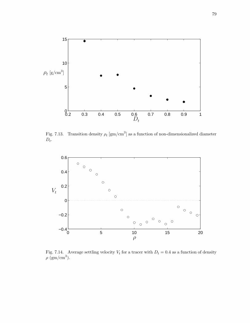
79
0.2 0.3 0.4 0.5 0.6 0.7 0.8 0.9 10
5
10
15
ρt [g/cm3]
Dt
Fig. 7.13. Transition density ρt [gm/cm3] as a function of non-dimensionalized diameterDt.
0 5 10 15 20−0.4
−0.2
0
0.2
0.4
0.6
Vt
ρ
Fig. 7.14. Average settling velocity Vt for a tracer with Dt = 0.4 as a function of densityρ (gm/cm3).

80
−200 −150 −100 −50 0 50 100 150 200
−50
0
50
100
150
−150 −100 −50 0 50 100 150 200
−50
0
50
100
−200 −100 0 100 200
−150
−100
−50
0
50
100
−300 −200 −100 0 100 200 300−300
−250
−200
−150
−100
−50
0
50
−40 −30 −20 −10 0 10 20 30 40
−40
−35
−30
−25
−20
−15
−10
−5
0
−60 −40 −20 0 20 40 60
−70
−60
−50
−40
−30
−20
−10
0
Fig. 7.15. Sample paths for a tracer of Dt = 0.4. Fifty paths are shown (moving left-to-right, top-to-bottom) for densities 5.3, 6.2, 8.1, 14.8, 15.7 and 16.7 g/cm3. Scale isshown in non-dimesionalized units on the horizontal and vertical axes of each plot.

81
linear. This can be seen in Fig. 7.16. In the case of ρ = 15.7 gm/cm3, the growth ofvariance over time is evidently linear (after a short initial period) as seen in Fig. 7.17.
A phase plot (Fig. 7.18) indicates regimes in which staircasing and diffusive behav-ior occur. There is a third regime where the variance in position remains fairly constantover time. This behavior (usually for higher values of ρ and Dt) can be understood byplotting sample paths which head down in a fairly straight line – the scatterers simplylack the momentum to move the tracer appreciably to the side. In the smaller, lighterend of the spectrum, we also see this direct rise behavior. Here, the tracers are pre-sumably light enough to be quickly slowed by the fluid. It is the middle regime wherestaircasing and diffusion can occur – where the tracer is dense enough to move somedistance through the fluid, but light enough to rebound noticeably from the scatterers.It would be interesting to know whether a transition (by varying the density or radius ofthe tracer) from staircasing to sinking in a straight line always passes through a regimeof diffusive behavior.
10−3
10−2
10−1
100
101
10−4
10−2
100
102
104
var(x)
t
Fig. 7.16. Variance of x-coordinates for 50 sample paths shown as a function of timefor spheres of Dt = 0.4 and ρ = 14.8 gm/cm3.
7.6.4 Sinking of a heavy sphere in bubbles
In the case of the heavier spheres the simulations show an apparent relationship
(see Figs. 7.19, 7.20) of VT − VT ∝ D−1/2t
ρ1/3, where VT is the terminal speed of thesphere in quiescent fluid. An estimate of VT can be based on the observation (seenin simulations and some experiments) that a heavy sphere can push aside bubbles tofollow a fairly straight path down with small side-to-side motions as it is pushed from

82
10−3
10−2
10−1
100
101
10−3
10−2
10−1
100
101
var(x)
t
Fig. 7.17. Variance of x-coordinates for 50 sample paths shown as a function of timefor spheres of Dt = 0.4 and ρ = 15.7 gm/cm3.
2 4 6 8 10 12 14 16 18 20
0.3
0.4
0.5
0.6
0.7
0.8
0.9
Dt
ρ
Fig. 7.18. Points marked with white squares show parameters where diffusive lateralmotion was observed, while black circles indicate tracers that rise or fall in fairly straightpaths. Gray triangles are used to show parameters where staircasing occurs.

83
10−0.4
10−0.3
10−0.2
10−0.1
100.2
100.3
Vt − VT
Dt
Fig. 7.19. VT − VT grows as D−1/2t
for ρ = 20 gm/cm3 (blue) and ρ = 19 gm/cm3 (red).A line of slope −1/2 is provided for reference.
100
101
10−0.3
10−0.1
100.1
100.3
Vt − VT
ρ
Fig. 7.20. VT − VT grows as ρ1/3 for Dt = 0.8 (blue) and Dt = 0.9 (red). Lines of slope1/3 are provided for reference.

84
one side and then the other by rising bubbles. We will then adapt Eq. 7.11 to representthe collision of a tracer with velocity x = (0,−Vt) and a scatterer with velocity (0, vB).This gives us
xR · n =−MVt +MBvB + eMB(vB +Vt)
M +MBsin θ (7.14)
where θ is the angle between the horizontal and the normal vector at the point of contact.Also we have
xR · t = Vt cos θ. (7.15)
The vertical component of the velocity after collision is then
−MVt +MBvB + eMB(vB +Vt)
M +MBsin2 θ −Vt cos
2 θ. (7.16)
The change in the vertical tracer speed of
−MVt +MBvB + eMB(vB +Vt)
M +MBsin2 θ −Vt cos
2 θ +Vt (7.17)
creates a vertical impulse of magnitude
M
(−MVt +MBvB + eMB(vB +Vt)
M +MBsin2 θ −Vt cos
2 θ +Vt
)
(7.18)
and, in a longer time scale, an effective acceleration of magnitude
M
τ
(−MVt +MBvB + eMB(vB +Vt)
M +MBsin2 θ −Vt cos
2 θ +Vt
)
(7.19)
where τ is the average time between collisions.It is natural to suppose that the average time between collisions is the time it
takes the tracer to move from one row of scatterers to the next. That is, we assume
τ =
√3
2
I +Ds
Vt + vB. (7.20)
We can support this conclusion by examination of the autocorrelation C(s) of the hori-zontal velocities Vx of the tracer as it settles. This is
C(s) =1
M − s
M−s∑
i=1
Vx(ti)Vx(ti + s)/C0(s) (7.21)
where C0(s) =1
M−s
∑M−si=1
Vx(ti)Vx(ti). If the tracer is being jostled from side to side,the correlation should change sign every s = τ . In Fig. 7.21 we show a small section ofC(s) for the tracer of diameter 0.9 and density 10 g/cm3 averaged over 50 runs. Thesign of the function changes every τ units, confirming our assumption.

85
0 2 4 6 8 10 12 14 16 18−1
−0.5
0
0.5
1
C(s)
s/τ
Fig. 7.21. The (average) autocorrelation C(s) of the horizontal velocities of a tracer(Dt = 0.9, ρ ≈ 10g/cm3) shows a regular reversing of velocity every τ units of time.
Replacing the sin2 θ and cos2 θ terms of Eq. 7.19 with their average values of 12 ,
we modify Eq. 6.3 to see that
M(Vt + vB)√3(I +Ds)
(−MVt +MBvB + eMB(vB +Vt)
M +MB+Vt
)
=4
3πr3
s(ρs−ρ)|g|−
1
2CDρV
2tπr2
s.
(7.22)We present solutions for Eq 7.22 for tracers of Dt = 0.9, 0.8 in Fig. 7.22. The resultsmatch qualitatively with the simulations at higher densities.
7.6.5 Autocorrelation
It is worth pausing here to note that the autocorrelation function for the horizontalvelocity of a tracer varies greatly depending on which phase of motion a tracer is in. Wehave seen in Fig. 7.21 the periodic autocorrelation of a sphere sinking mostly downwardswith a small back-and-forth motion. For a tracer that is staircasing, the horizontalvelocity remains (on average) fairly constant. This produces an autocorrelation thatdoes not die off with time as seen in Fig. 7.23. For a tracer in diffusive motion, thecorrelation dies off quickly. In the case of Fig. 7.24 we see that this take about thepassage time for 10 scatterers, so presumably about 10 collisions.
7.7 Simulation results: added velocity
In the fluid Galton model and simulation of sections 7.4 and 7.5 one can think of asmall, light tracer that, instead of colliding with the scatterers is advected around them.

86
100
101
10−0.3
10−0.1
100.1
Vt − VT
ρ
Fig. 7.22. VT − VT simulated (circles) and estimated (+) by Eq 7.22 for Dt = 0.8 (blue)and Dt = 0.9 (red).
0 10 20 30 40 50 60 700
0.5
1
1.5
C(s)
s/τ
Fig. 7.23. The (average) autocorrelation C(s) of the horizontal velocities of a tracer
(Dt = 0.4, ρ ≈ 10g/cm3) in a staircasing regime reflects its continued linear path byremaining near 1.

87
0 5 10 15 20 25 30−0.2
0
0.2
0.4
0.6
0.8
1
1.2
C(s)
s/τ
Fig. 7.24. The (average) autocorrelation C(s) of the horizontal velocities of a tracer(Dt = 0.4, ρ ≈ 2.4g/cm3) in a diffusive regime dies off quickly.
In the model and simulation as described, there is no fluid motion taken into accountthat is not uniform (i.e. an overall circulation velocity) and this effect is not seen. Wewished to find some approximation for the non-uniform component of fluid flow directlyaround the scatterers and observe its effect on the simulations. To this end we createdan added velocity in the fluid about each scatterer.
The flow induced by a single rising spherical bubble is close to potential flowaround a sphere – especially on the upstream side of the bubble where collisions tend tooccur. To create an added velocity for the multiple scatterers, we simply sum the dipolesshown in Eq. 5.17. This is, of course, not the same as the potential flow calculated formultiple spheres simultaneously, in that it does not satisfy the appropriate boundaryconditions at either the scatterer or tracer surfaces. However, it seems appropriate tothe simplicity of our model.
Now we will modify Eq. 7.10 for the tracer for a situation in which u 6= 0 to
(m+mA)x =4
3πr3
s(ρ− ρs)|g|k +
1
2CDρπr
2s|u− x| (u− x) . (7.23)
It is not immediately clear, however, what value of fluid velocity u should be used inEq. 7.23. For instance, using the value at the center of the tracer is undesirable becausethe velocity given by Eq. 5.17 drops off quickly (at slowest, on the order of 1
|x|3 ) away from
the surface of a scatterer. So to measure u at the center of a tracer of larger radius mighthave very little effect. Also because the field drops off rapidly with distance (and canalso change rapidly by changing the angle between the tracer and the axis along which

88
the scatter moves) the effect on the tracer would become sensitive to small changes inlocation.
We determined to use for u an average velocity over the volume of the sphere.This is similar in some sense to the case where a tracer moves in a uniform flow, andthe value of u is the same as the average over the volume of the sphere of the flow as itwould have been without the presence of the tracer. This is a very rough estimate, butperhaps commensurate with the nature of the velocity field we have chosen.
The results are qualitatively the same as without the added velocity terms. Forexample, in Fig. 7.25 we see the same trend of a floating to falling transition withincreasing density. We also see the transition from staircasing to diffusive lateral motion.An example of this is shown in Fig. 7.26. This does indicate that the staircasing behaviorseen in the previous section has some insensitivity to small perturbations.
It is interesting to note that the transition from staircasing to diffusive motionis not a sudden one, but characterized by staircasing with a small number of tracersin apparently diffusive motion. It appears that the beginning motions of the tracers inthe staircasing regime are much the same as those after the transition. However, thetracers appear to have a chance of entering a steady staircasing state over time. This isnot unique to simulations with the added velocity effect, but is seen also in the previoussection. This helps explain, for instance, the small amount of time in Fig. 7.16 where thevariance appears to grow linearly – most of the tracers may still be moving diffusivelyat this point. A detail of the these paths changing from diffusive to staircasing behavioris shown in Fig. 7.27.
5 10 15 20 25
−0.6
−0.4
−0.2
0
0.2
0.4
0.6
Dt=0.3
Dt=0.35
Dt=0.4
Dt=0.45
Dt=0.5Vt
ρ
Fig. 7.25. Average settling velocity Vt as a function of density ρ [gm/cm3]. The trendsare similar to those seen in Fig. 7.12.

89
4 6 8 10 12 14 16−0.3
−0.25
−0.2
−0.15
−0.1
−0.05
0
0.05
0.1
Vt
ρ
→ diffusive→ mixed ←staircasing ←
Fig. 7.26. Average settling velocity Vt for a tracer of diameter Dt = 0.45 as a function ofdensity ρ [gm/cm3]. Tracer paths still transition from staircasing to diffusive behavior.
−60 −40 −20 0 20 40 60
−40
−30
−20
−10
0
10
Fig. 7.27. A detail of 50 sample paths for a tracer of Dt = 0.4 and density ρ =14.8 g/cm3. An image of these paths at a larger scale is found in Fig. 7.15.

90
Chapter 8
A sphere sinking in bubbles:
experimental measurement of collision effects
8.1 Experimental setup
To be able to observe the effects of collisions and do experimental comparisonwith the simulations described in chapter 7, we decided to perform another experimentin which collisions would be highlighted. The primary goal is to measure the lateralmotion and test for diffusive behavior. We refined the experimental setup describedin chapter 6 as follows. First we narrowed the cell in which the spheres were to fall.The purpose to this was to create a cell slightly larger than the ascending bubbles. Thiscreates a single layer of bubbles in which the risk of obscuring the sphere is much smaller.Conversely, because the sphere cannot easily pass before or behind a bubble, the chanceof a collision is higher.
In the new experiment, the cell is constructed of two acrylic plates of dimensions0.64 cm×23.2 cm×30.5cm (14
′′ × 918′′ × 12′′). The front sheet is transparent, while the
back sheet is translucent to help diffuse light. The acrylic plates slot into aluminumplates in channels separated by 0.32 cm (18
′′). Because the cell is wider than the bubbler,
weighted inserts were made to insert into the cell to close the ends of the experiments.(If the edges of the cell are not closed, the overall flow becomes irregular.)
We decided to use a small, light sphere so that the collisions with bubbles wouldbe more evident. This also has the benefit of avoiding situations in which bubbles arelikely to be trapped in the wake of the spheres. For the material of the sphere wedetermined to avoid plastics and rubber, which were materials we had seen attach tobubbles in our first experiment. We chose to use aluminum spheres of 3
32” diameter
(0.24 cm, McMaster-Carr aluminum alloy 2017, density 2.8 g/cm3).One area of great interest to us was to make a uniform field of bubbles; that
is, a bubble field in which the bubbles sources were evenly distributed and the bubblesizes were monodisperse. In this we decide to follow the work of R. Zenit who producesmonodisperse bubble fields using banks of capillaries (see e.g. [100]).∗ To prevent poly-dispersity through the coalescence of bubbles, Zenit also adds MgSO4 to the fluid (bothwater and water-glycerol mixes). At a concentration of 0.05mol/l, this inorganic salthelps prevent bubbles form coalescing (a common phenomenon in our previous exper-iment) by creating a short-range (hydration) force between the bubbles. However, itdoes not at these concentrations substantially alter the surface tension of the bubbles, orchange the density or viscosity of the fluid [100]. At his advice, we also began to supply
∗As we experimented with capillary banks, we noticed an interestingly-shaped bubble plumewhich we describe in appendix D.

91
gas from a Nitrogen tank to avoid the possibility of introducing oil from the compressorinto the system.
To create the capillary bank, we initially used glass capillaries (Drummond Mi-crocaps, length 5.5 cm, inner diameter 0.015 cm), which produced uniform bubbles ofDt = 0.21 cm. The capillaries were put in arrays in acrylic sheets, and held in placewith casting acrylic. An example of the bubble field generated by such an array is shownin Fig. 8.1. While experimenting with these capillaries, we came across the interestingphenomenon of hourglass-shaped bubble plumes which will be described in appendixD. Unfortunately, despite much care, the capillaries were very prone to breaking andimpossible to replace in the array once broken.
Fig. 8.1. Bubbles produced uniformly by a bank of nitrogen-fed glass capillaries.
We replaced the glass capillaries with stainless steel needle-tubing that had beencut flat and deburred (Vita Needle, length 3.8 cm, inner diameter 0.015 cm). Forty-fiveneedles were spaced evenly in an acrylic sheet with a separation of 0.37 cm. The heightswere staggered by 0.32 cm to prevent the possibility of coalescence of the bubbles whilethey were forming on the needles. Also, the needles were glued on the top with super-glue so that they could be removed and replaced if necessary. The new arrangement isshown in Fig. 8.2.
Our initial reaction was disappointment: although the needles had the same innerdiameter as the glass capillaries, the bubbles produced had much smaller diameters (afactor of about two). To increase the size, we treated the surface of the needles tomake them hydrophobic. Our first attempts with rain-repellent for cars produced largerbubbles, but quickly wore off of the needles. We found success with Dow Corning high

92
Fig. 8.2. The capillary bank of stainless steel needle tubing.
vacuum grease (a silicon lubricant). Larger bubbles were produced and the product isstable for the course of experiments, the results are shown in Fig. 8.3. Before a runof experiments the needles are cleaned and re-greased. The grease is thick enough toclog some of the needles, but this is remedied by suctioning individual needles. Care istaken to clean the spheres after an experiment, as there is some transfer of grease fromthe needles when the reach the bottom of the cell. If not removed, this leaves themsusceptible to having bubbles attach to them regardless of the material.
8.2 Experimental Results
8.2.1 Settling Velocity
The average y position of 50 experiments shows a linear trend as shown in Fig. 8.4,along with a fit of the data. The settling velocity VT is 3.9cm/s. Note that the length ofthe runs varied from a little over three seconds to more than the camera’s buffer lengthof about 13 seconds. The average recorded length was 6.5 s. In this analysis, we haveused only 3.6 seconds of data as this was the length of the shortest run. A set of 25experiments on spheres of Ds = 5/64” similarly yields a settling speed of 1.8352 over asample period of about 6 s.
We wished to determine the circulation velocity in the cell, so that this could besubtracted from the terminal velocity of spheres sinking inside the cell but in quiescentfluid. The difference between this and the settling speed is likely caused by collisionbetween the sphere and the bubbles. We can infer - based on our experiment describedin Chapter 6 that the circulation velocity is the difference between the speed of a singlebubble rising in the cell and the rise velocity of the bubbles in the bubbly fluid.
We measured the average rise velocity of bubbles rising singly through the celland found a velocity of 18.8 cm/s. For bubbles rising in the array we measure an averagerise velocity of 34.4 cm/s. We therefore estimate a circulation velocity of 15.6 cm/s.

93
Fig. 8.3. The bubble field produced by the stainless steel capillaries. The inset in theupper-right shows (to scale) bubbles from the untreated capillaries.
The settling velocities of the larger and smaller spheres in quiescent water in thecell we measured respectively at 29.4 cm/s and 26.8 cm/s. The effect of circulation aloneshould bring the settling velocities to 13.8 cm/s and 11.2 cm/s. Thus we estimate theslowing effect of the collisions to be 9.9 cm/s and 9.4 cm/s respectively.
8.2.2 Diffusivity
Paths from the first 3.6 s of the 50 runs for Ds = 3/32” are shown in Fig. 8.5.The starting positions of the recorded paths are placed at the origin. The single runrising up above the origin was unusually long and the path recording began well belowthe top of the cell. There is a noticeable outward spread and the lateral motion doesappear to be diffusive. The growth of variance over time is shown in 8.6 with a fit ofy = 0.59x+ 0.02. This translates to a coefficient of diffusion of D = 0.30. Note that thevariance of the sample variance is proportional to the square of the variance [6] whichmay explain the growing fluctuations in the variance about the linear fit. The spheresof Ds = 5/64” have a coefficient of diffusion of D = 0.35.
We can visually compare sample paths for the larger spheres to solutions of Φt =
0.3Φxx with initial condition Φ(x, 0) = 50δ(x). The solution is Φ(x, t) = 50√1.2πt
exp(
− x2
1.2t
)
.
Propagated downward at velocity 3.9 this becomes
Φ(x,−y) = 50√
1.2πy/3.9exp
(
− x2
1.2y/3.9
)
(8.1)
as shown in Fig. 8.7.
8.2.3 Staircasing
As staircasing was a prominent feature of the model results, we wished to knowwhether the phenomenon was seen experimentally. The answer is that staircasing doesoccur, but on a much smaller scale. For example, the sphere in 8.8 shows short instancesof staircasing. The instance ends when the sphere runs into a larger gap between bubbles.

94
0 0.5 1 1.5 2 2.5 3 3.5 4−15
−10
−5
0
〈y〉
t
Fig. 8.4. Average vertical position 〈y〉 [cm] as a function of time [s] for spheres ofdiameter Dt = 3/32”. This is shown along with a fit of y = −3.9t− 0.18.
The staircasing behavior in simulations is very dependent on the regularity of the arraysand such short instances are as much as we might reasonably expect.

95
−5 0 5
−25
−20
−15
−10
−5
0
Fig. 8.5. Experimentally observed paths. Data are shown for 50 paths over about 3.6seconds for spheres of diameter Ds = 3/32”.

96
0 0.5 1 1.5 2 2.5 3 3.5 40
0.5
1
1.5
2
2.5
var(x)
t
Fig. 8.6. Variance in the x-coordinate of position as a function of time. Data are shownfor 50 paths over about 3.6 seconds for spheres of diameter Ds = 3/32”. Also shown isa fit of y = 0.59x+ 0.02.
−5 0 5−10
−8
−6
−4
−2
−5 0 5−10
−8
−6
−4
−2
Fig. 8.7. Comparison of sample paths with a solution to diffusion. See text for details.

97
Fig. 8.8. The path of a sphere (Ds = 3/32”) (shown in yellow) shows short instancesof staircasing.

98
Chapter 9
Conclusion and future directions
9.0.4 Fragmentation of a 1-D rod
In the beginning of this work, we examined the mathematics describing the frag-ments produced by breaking a one-dimensional rod. We were able to provide models inthe case of fragmentation of either a discrete or continuum rod. The continuum modelwas found to be capable of producing scaling, which is important as power laws describethe distribution of fragment sizes in many different circumstances. We also found thatthis model provided satisfactory qualitative results when compared to experiment.
The continuum model corrects a commonly accepted model for fragment sizes aris-ing from a homogenous Poisson process. The misunderstanding seen in the presentationof the extant model seem to typify errors made in more complex analyses.
In the future there are two important additions that could be made to this work.The first would be to relate the physical state of a rod to its probability of breaking. Thesecond would be to extend the one dimensional model to two or three dimensions. Ofthese two, we became interested in the fragmentation in higher dimensions. Although thequestion of geometry and crack intersection becomes very difficult in two dimensions,there may be some promise in pursuing fragments distributions that are created asVoronoi tessellations.
9.0.5 Spheres sinking in bubbles – a proposed continuum model for path-
clearing
In the latter part of this work we examined the motion of a sphere settling ina bubbly fluid. We found that water circulating with the bubbles must be taken intoaccount when trying to determine the effects of the bubbles on the spheres. By refiningour experiment we were able to examine the effect of bubble collisions with small, lightspheres. Two effects of these are a further slowing of a sphere’s descent in the liquid,and lateral diffusive motion of the spheres.
Based on similarities with the classic Galton board, we created a model for afluid Galton board and demonstrated the occurrence of these two effects (slowing anddiffusion) in simulations. We also found parameter ranges in which staircasing – thediagonal descent of a sphere as if down a staircase – may occur.
One useful extension of this model would be to determine what the effect ofmultiple tracers would be on the model. Heuristically, one might expect that manytracers released over time from a central source might clear a path through the risingbubbles so that those following experienced fewer collisions. Perhaps this sort of path-clearing can come, not from the fluid Galton model, but from an expanded version of

99
Galton’s model of random left-right steps. We present a model of this sort, combining arandom lateral movement of the tracer with partially mobile scatterers.
We assume that there is a population of tracers with (number) density T (x, z, t) cm−2
and a population of scatterers with density S(x, z, t) cm−2. We will reduce the scatterersonce more to point particles for convenience and let the radius of the tracer be rt. Wewill furthermore allow the tracers to interact only with scatterers, and likewise scatterersto interact only with tracers.
The tracers will move down at a steady speed v. In principle we might let v =v(S), but for now we will assume this is constant. At each collision of a tracer with ascatterer the tracer will move to the left or right a distance LT , each with probability 1
2 .The scatterer will be moved in the opposite direction a distance of LS. Thus, after 2Ncollisions, the probability that the particle has moved to the right a distance of 2MLT
is(
1
2
)2N ( 2N
M +N
)
. (9.1)
A similar expression is available for an odd number of collisions. In either case, thestandard deviation of the distance moved after N collisions is
σ =LT
2
√N. (9.2)
A tracer moving with velocity v will sweep out new area at a rate of 2rT |v| perunit time. We take this to be approximately 2rT v, and take the expected number ofcollisions in time ∆t to be
E(N) = 2rT v∆tS. (9.3)
The rms lateral displacement in time ∆t of a tracer based on this number is
σ =LT
2
√
2rT v∆tS. (9.4)
This can also be derived a more rigorously by saying that we take the scatterers to bedistributed according to a Poisson process with density S and finding the variance of thedisplacement for N and M .
We will now parallel a derivation for the flux of tracers per unit time through avertical line following the derivation of Einstein (1907) [23] – the main differences in ourargument being that the particles with random lateral motion are also moving downwardat a constant rate, and are being scattered by a non-uniform population. To begin with,we will make our calculations as if all the tracers moved a distance σ in time ∆t. Now fixa vertical line going through x0. We replace the quantities T and S with the quantities
T (x) = 1
∆z
∫ z0+∆z
z0
T dz
and
S(x) = 1
∆z + v∆t
∫ z0+∆z+v∆t
z0
S dz.

100
We establish rectangles to each side of the line with width σ and height ∆z,centered at (x0 ± σ/2, z0 +∆z/2− vt, t0 + t). In time ∆t, half of the tracers in the boxto the left of the line will move across the line to the right. Similarly half of the tracersin the box to the right will cross to the left. With T ± = T (x0 ± σ/2), this gives a netflux of approximately
1
2
(
T + − T −)
σ∆z =1
2
(
T + − T −)
σσ2∆z (9.5)
across a segment of the line of height ∆z. In other words, the rate of flux per unit heightper unit time is
1
2
σ2
∆t
(
T + − T −)
σ. (9.6)
Letting ∆z and then ∆t go to zero we see that the flux across the line is
J(x, z, t) = −1
4L2TrT vS(x, z, t)
δT (x, z, t)
δx(9.7)
per unit time per unit distance.We proceed with a standard conservation of mass approach to find that
T (x, z − vdt, t+ dt)− T (x, z, t) ≈ −dt∂J∂x
= dt1
4L2T rT v
δ
δx
(
SδT
δx
)
. (9.8)
so thatδT
δt− v
δT
δz=
1
4L2T rT v
δ
δx
(
SδT
δx
)
. (9.9)
Note that if S(x, z, t) = S0, then this describes (in the rest frame of the tracers) thelateral diffusion
δT
δt=
1
4L2TrT vS0Txx.
For the evolution of S, we likewise examine the flux through a vertical line throughx0. Take a small rectangle of width dx and height vdt. In time dt there are vTdxdttracers traveling (in a cumulative sense) the height of the box. This produces a totalof 2rT v
2STdxdt collisions. To establish (as we did for the tracers) a common distancetraveled by each scatterer we assume that each scatterer is hit an equal number of times.This is then
N = 2rT v2STdxdt/ (vSdxdt) = 2rT vT (9.10)
so that for the scatterers, the rms distance traveled per unit time is
σS =LS
2
√
2rT vT . (9.11)
Similarly to the above,
JS(x, z, t) = −1
2σ2S
δS
δx= −1
4L2SrT vT
δS
δx(9.12)

101
andδS
δt=
1
4L2SrT v
δ
δx
(
TδS
δx
)
. (9.13)
This is similar to 9.9 with the exception that there is no vertical transfer. As before, ifT is constant in x, this simply becomes the diffusion
δS
δt=
1
4L2SrT vTSxx. (9.14)
This, in fact, is what leads us to speculate that path-clearing may occur: if we havea source of tracers, T will be fixed along the line of insertion, positive at the place ofinsertion and zero elsewhere. The scatterers below the source will be mobile, while thoseelsewhere will not be as mobile. This may lead to a decrease of the scatterers below thesource, and allow the concentration of tracers to propagate downwards.
We have derived a coupled PDE model
δT
δt− v
δT
δz=
1
4L2TrT v
δ
δx
(
SδT
δx
)
δS
δt=
1
4L2SrT v
δ
δx
(
TδS
δx
)
.
(9.15)
Individually these equations are those of heat conduction with a variable thermal con-ductivity. It remains to find solutions either analytically or numerically and see if path-clearing occurs and if this resembles the fluid Galton model with many successive tracers.

102
Appendix A
Coefficient of restitution
In this appendix we will closely follow the presentation of Stronge [91] on rigidbody impact, although our work will be much simplified in that we will consider onlycollisions between smooth spherical particles. We have spheres one and two with veloc-ities V1, V2 and masses m1, m2. First consider a direct impact in which the relativevelocities are parallel to the normal vector at the point of collision as in Fig. A.1. Be-cause the components of motion and acceleration are along one axis, we shall write themas scalars.
n
V1V2
Fig. A.1. A direct collision.
From the conservation of momentum, the impulse imparted to each particle isequal in magnitude and opposite in direction. Then we can write the velocities from thetime of impact t0 as
V1(t) = V1(t0) +1
m1P (t) (A.1)
and
V2(t) = V2(t0)−1
m2P (t). (A.2)
(Note that this implies P (0) = 0.)The centers of the particles move closer together until the time tc when the ve-
locities are equal, i.e.
V1(t0) +1
m1P (tc) = V2(t0)−
1
m2P (tc) (A.3)

103
so that(
1
m1+
1
m2
)
P (tc) = − (V1(t0)− V2(t0)) . (A.4)
The work done during this time is
Wc =∫ tc0
FV1 − FV2 dt
=∫ tc0(V1 − V2) (Fdt)
=∫ P (tc)0
(V1 − V2)dP
=∫ P (tc)0 (V1(t0)− V2(t0)) +
(
1m1
+ 1m2
)
P dP
= (V1(t0)− V2(t0))P (tc) +12
(
1m1
+ 1m2
)
P (tc)2
= − m1m2m1+m2
(V1(t0)− V2(t0))2 + 1
2m1m2m1+m2
(V1(t0)− V2(t0))2
= −12
m1m2m1+m2
(V1(t0)− V2(t0))2.
(A.5)
During this time, a small volume of the colliding particles is deformed and someof the energy from the deformation may be stored elastically, causing the spheres torebound from each other. This process will take place from time tc to time tf doing thework
Wr =∫ P (tf )
P (tc)(V1(t0)− V2(t0)) +
(
1m1
+ 1m2
)
P dP
= (V1(t0)− V2(t0))(P (tf )− P (tc)) +12
(
1m1
+ 1m2
)
(
P (tf )2 − P (tc)
2)
= − m1m2m1+m2
(V1(t0)− V2(t0))2(
P (tf )P (tc)
− 1)
+ 12
m1m2m1+m2
(V1(t0)− V2(t0))2(
P (tf )P (tc)
2− 1)
= 12
m1m2m1+m2
(V1(t0)− V2(t0))2(
P (tf )P (tc)
2− 1− 2
P (tf )P (tc)
+ 2)
= 12
m1m2m1+m2
(V1(t0)− V2(t0))2(
P (tf )P (tc)
− 1)2
.
(A.6)The coefficient of restitution is the root of the proportion of the restoring work to thecompressing work, i.e.
e2= −Wr
Wc=
(
P (tf )
P (tc)− 1
)2
. (A.7)
The coefficient of restitution defined as
e =P (tf )− P (tc)
P (tc)(A.8)
is called the kinetic coefficient of restitution, and dates to Poisson in 1811. We can alsouse Eqs. A.1, A.2, A.4 to obtain
e = −V1(tf )− V2(tf )
V1(t0)− V2(t0)(A.9)
which is the kinematic coefficient of restitution proposed by Newton in 1686. In thesituations we are considering, these are equivalent.

104
From Eq. A.9 we have
V1(tf )− V2(tf ) = eV2(t0)− eV1(t0). (A.10)
From conservation of momentum we have
V2(tf ) = V2(t0) +m1
m2(V1(t0)− V1(tf )). (A.11)
Together these give us
V1(tf )− V2(t0) +m1
m2(V1(tf )− V1(t0)) = eV2(t0)− eV1(t0) (A.12)
so thatm2 +m1
m2V1(tf ) = (1 + e)V2(t0)− eV1(t0) +
m1
m2V1(t0) (A.13)
andV1(tf ) = m2
m2+m1((1 + e)V2(t0)− eV1(t0)) +
m1m2+m1
V1(t0)
= m1V1(t0)+m2V2(t0)+em2(V2(t0)−V1(t0))m1+m2
.(A.14)
Because tf−t0 is very small, we will consider the collisions to be instantaneous and writeV1(t0) = vI , V1(tf ) = vR and V2(t0) = uI , V2(tf ) = uR. So that
vR =m1vI +m2uI + em2(uI − vI)
m1 +m2. (A.15)
For an equation in which there are normal components to the velocity as inFig. A.2 the situation is generally more complicated. However, because we are suppos-ing the particles to be smooth (in this sense, to pass without sticking or friction) thetangential components of forces between the spheres are zero. In this case, the tangen-tial velocities remain unchanged. In this case (with t in the direction of the tangentialcomponent of vI)
vR · t = vI · t (A.16)
and
vR · n =m1vI · n+m2uI · n+ em2(uI · n− vI · n)
m1 +m2. (A.17)
If the second sphere is fixed in position, it has no velocity and can be treated asa particle of infinite mass. In this case Eq. A.17 becomes
vR · n = −evI · n. (A.18)

105
vI
vR
n
t
uI
uR
Fig. A.2. An oblique collision.

106
Appendix B
A coefficient of restitution
for bubbles, drops, and particles
In our simulations a simple coefficient of restitution was used for the reboundof the spheres and bubbles. A more realistic coefficient of restitution would depend oncharacteristics of the collision such as the Stokes number (provided later in this section)and the capillary number Ca = µU/σ (where σ is the surface tension of the bubble).Although the nature of a coefficient of restitution for a bubble and sphere is unknown atthis time, we provide here a review of literature discussing what is known about using acoefficient of restitution to describe the rebound of submerged solid spheres, drops andbubbles.
B.1 Approach and rebound of two spheres
Ironically, the first predictions for a submerged coefficient of restitution were de-veloped by researchers interested in criteria for particles to remain together after collisionin a fluid. In 1986, Davis, Serayssol and Hinch [21] modeled the collision of two smoothelastic spheres in a fluid of constant viscosity and density. Their analysis shows howhigh pressure in the inter-particle gap may cause deformation of the spheres, leading toa rebound.
Much of the work in their paper and in subsequent research from members of thisgroup and their colleagues [83, 7, 8, 9, 20] focuses on the forces between two approachingspheres in a viscous fluid and the corresponding deformation of the spheres. Although wewill not expand our review to the more general question of the approach of two spheres,we will consider these papers as they lay a foundation that provides important results indescribing a submerged coefficient of restitution. The theoretical work by the precedingauthors has been examined in experiments with collisions that are not fully submerged.
The initial analysis of Davis [21] was used and expanded in subsequent papers[83, 7, 8, 9, 20]. In their analysis, two spheres of radii a1, a2 approach each other in aviscous fluid. It is assumed that very little deformation occurs until the inter-particlegap is small enough that the lubrication equation
∂h
∂t=
1
12µr
∂
∂r
[
rh3∂p
∂r
]
(B.1)
holds. Here h is the inter-particle gap parallel to the axis of the two spheres, andmeasured at a radius r from the axis. The profile of the spheres are approximated by

107
parabolas, so that the gap h can be written (see Fig. B.1)
h(r, t) = x(t) + w(r, t) +r2
2a(B.2)
where x is the distance that would have existed between the undeformed surfaces, wis the sum of the deformations of the two surfaces and a is the reduced radius of thespheres (i.e. a = a1a2
a1+a2). Note that one of the radii may be set to ∞ to describe the
collision of a sphere with a wall.
x(t)
w1(0, t)
w2(0, t)
Fig. B.1. The undisturbed (dotted lines) and physical profiles (solid lines) of two spheresshow the centerline distance x(t) and the deformation w(r, t) = w1(r, t) + w2(r, t).
Describing the gap in this manner allows a coupling with the motion of the spheres
dx
dt= −v(t), m
dv
dt= −F (t) (B.3)
where m is the reduced mass of the spheres, and the force F is found by integratingsurface forces (assumed to act equally on the two surfaces.) In the initial analysis, thisis the hydrodynamic pressure. ( Gravity is ignored as its effect is of a smaller order ofmagnitude based on typical Froude numbers.)
Later papers considered the contribution of other sources of interparticle force.Serraysol and Davis [83] (with an eye to colloids and aerosols) considered the addition ofLondon-van der Waals and electrical double layer forces. However, in the case of reboundleading to separation of the particles (the case of interest to us) they conclude that
For particles that have sufficient inertia to deform and rebound, the electricaldouble layer repulsive forces, and the potential barrier between the primary

108
and secondary minimum, are negligible during the collision process for allcases of practical interest.
Barnocky and Davis [7] considered effects based on the observation that in air, the meanseparation between the spheres considered by Davis [21] could be on the order of severalnanometers – smaller than the mean free path of the air molecules. They account fornon-continuum effects by adjusting the no-slip boundary conditions of the continuumequations. This reduces the magnitude of interparticle forces, allowing them to drawmuch closer or even collide. However the results are again not applicable to a liquid,whose molecules have a much shorter mean free path. Davis [19] discusses both ofthese effects with a small section on the effect of surface roughness, modeled as smallhemispheres attached to the larger, colliding spheres. He concludes that for an examplecase, the hydrodynamic effect of the hemispheres is unimportant up to the point wherethey begin to touch and support the other sphere.
Returning to the initial analysis of Davis [21], the deformation of the sphereswas coupled to the interparticle forces through the experimental parameters of Young’smodulii and Poisson ratios. By non-dimensionalizing, two parameters governing therebound of the sphere were identified: the particle Stokes number
St =mv06πµa2
(B.4)
– a measure of the relative effect of particle inertia and viscous dissipation in the fluid (asopposed to the Reynolds number which considers the fluid inertia) – and the elasticityparameter
ε =4θµv0a
3/2
x5/20
(B.5)
where
θ =1− ν21πE1
+1− ν22πE2
(B.6)
is derived from the Young’s modulus Ei and Poisson’s ratio νi for each sphere, and x0, v0are initial separation and velocity at which deformation is considered to begin. In theinitial consideration a typical value for ε is given as 10−7 to 10−5 (based on 10− 100 µmsandstone particles in water.) For comparison, later experiments in which steel and nylonballs of a = 0.32 to 0.64 cm were dropped onto a quartz disk have elasticity parameterson the order of 10−6 to 10−4 and 10−3 to 10−2 respectively [20].
There are two critical findings derived from their analysis (based on asymptoticanalysis for small deformations and numerical analysis for larger). The first is that thereis a critical Stokes number below which no rebound occurs. This number is based off ofthe elasticity parameter and can be taken to be [20]
Stc = −0.4 log(ε)− 0.2. (B.7)
For the values of ε mentioned here, this ranges from about 1 to 7.Barnocky and Davis [8] verified the existence of the critical Stokes number ex-
perimentally by dropping stainless steel and lucite spheres (a = 0.8 to 3.2 mm) onto a

109
quartz disk covered with a thin layer of oil. By measuring the dropping height at whichthe spheres rebounded for varying oil depths and viscosities, they measured the criticalStokes number and found favorable comparison to their (slightly different) prediction of
Stc = −0.5 log(ε)− 1.3. (B.8)
Davis, Rager and Good [20] found similar agreement with experiments using stainlesssteel and nylon spheres. They noted that their measured values of Stc were generally toolow for small values of 1/ε (for which the spheres do not penetrate very far into the oillayer), but that in this case the analysis does not hold as the requirement that ε << 1is not met.
Alternately, for large values of 1/ε the measured values of Stc were higher thanpredicted. This could be [8] because the analysis predicts a rebound, not necessarilyenough of a rebound to visibly exit the oil layer. The rebounding sphere is also subjectto tensile stress as it moves away from the wall. However, a typical pressure drop ofseveral hundred atmospheres may cause cavitation and mitigate this effect. This couldalso be [20] from an initial deformation of the sphere as it first penetrates the oil, beforethe point at which the original analysis assumes the beginning of deformation.
The second finding of Davis [21] is that the non-dimensionalized (maximum) re-bound velocity vr
v0may be thought of as a coefficient of restitution. This coefficient of
restitution was explored numerically for a variety of ε through Stokes numbers of aboutSt = 30. The coefficient of restitution is seen to remain near zero until the critical Stokesnumber, after which it increases rapidly. In their experiments with stainless steel andnylon spheres, Davis [20] measured the coefficient of restitution. To account for energydissipated by the spheres and quartz, the coefficient of restitution is multiplied by the“dry” coefficient of restitution to get
e = edry
(
1− StcSt
)
. (B.9)
The data collapse convincingly to this master curve with no free parameters. This curveis shown in Fig. B.2.
Another experimental study on a wet coefficient of restitution using a thin oilcoating is due to Lundberg and Shen [61]. In this experiment, a roller attached to theend of a pendulum arm was allowed to strike a sphere resting on a piezoelectric sensor.The coefficient of restitution was measured both by comparing incoming and outgoingvelocities using an accelerometer in the pendulum, and by integrating the forces beforeand after the instant of rebound. A drop of oil placed on the sphere provided the lu-brication layer. It is difficult to compare results, as Lundberg presented the normalizedcoefficient of restitution (e/edry) for several impact velocities as a function of the viscos-ity of the applied oil rather than using the Stokes number. Lundberg showed that thecoefficient of restitution generally decreases with increasing viscosity (as should be ex-pected for a decreasing Stokes number) and that the effect is more pronounced for nylonthan for steel (also expected from the theory of Davis, as the coefficient of restitutionincreases more rapidly at smaller Stokes numbers). An interesting note from Lundberg’s

110
100
101
102
103
0
0.2
0.4
0.6
0.8
1
St
e/edry
Fig. B.2. The master curve of Davis, Rager and Good for values of the normalizedcoefficient of restitution [20]. In principle the value of Stc varies by material. Here weshow a commonly described value of 10.
study is a measurement of the wet coefficient of restitution above that of the dry. Theyalso show trends where the coefficient of restitution increases with increasing viscosity.
Returning once more to the study of Davis, Serayssol and Hinch [21], anotherquantity that was calculated was the minimum distance of approach for two spheres.They noted (correctly as will be seen in later experiments) that their analysis maybe problematic in cases where the surface roughness is of a comparable length to theminimum distance of approach. Later experiments, both those of Barnocky and Davisas well as experiments involving fully submersed collisions showed the effects of surfaceroughness.
Barnocky and Davis [9] extended the results of Davis by allowing viscosity anddensity of the interstitial fluid to vary with pressure - which in other experiments hadbeen found to be as high as several hundred atmospheres. In their approach
ρ
ρ0= 1 +
αp
1 + 3α|p| (B.10)
where ρ0 is the fluid density at ambient pressure, and α is an experimental compressibilityparameter (typically O(10−4) atm−1). Viscosity is allowed to vary as
µ = µ0(1 + βp)16 (B.11)
where µ0 and β are similarly viscosity at ambient pressure and an experimental param-eter.

111
Their analysis showed that one effect of increased density with pressure is to storea small amount of energy. They noted that this might make a rebound possible even forrigid spheres. In the case of elastic spheres, the effect is to increase the deformation ofthe spheres and enhance the rebound. Increased viscosity does not store energy in thesame way, but does also enhance the rebound by making the fluid harder to evacuate forthe interstice – essentially making the fluid act more like a solid.
The general predictions for the coefficient of restitution are qualitatively similarto the ones mentioned before – a critical Stokes number below which no rebound occursbut above which the coefficient of restitution increases rapidly.
Attempts were made to simplify the equations of motion presented by Davis [21].Wells [95] presented an approximation to sphere deformation designed to preserve thenormal force on the spheres. In an inner region, the profile of the sphere is consideredto be flat, while outside this region the deformation decreases to zero as the radiusincreases. This loses some features of the deformation profile as described by Davis,such as a dimple on the axis of approach. However, in this way he reduces the equationsof motion for the sphere to a fourth order system of ODEs. The calculated coefficient ofrestitution is similar to that of Davis for small values of St, but increases more rapidlybeyond Stokes numbers of about St = 15.
In 1996, Lian, Adams and Thornton [58] proposed a further simplification to thetheory of Davis [21]. In their model, the profile of the approaching spheres was assumedto be flat within a central region similarly to Wells [95]. Outside of this region, however,the deformation of the sphere profile was taken to be constant. This allowed for ananalytic evaluation of the force on the spheres, which for Davis and Wells was onlyavailable numerically for all but small deformations. Lian showed that for purposes ofmeasuring the coefficient of restitution, their approximation fits the calculations of Davisvery well. Note, however, that this deals with Stokes numbers of up to about 30 – twoorders of magnitude smaller than much of the experimental data discussed previouslyand hereafter.
B.2 Submersed collisions
Experimental work on a fully submerged coefficient of restitution began to bepublished in 1999 in a brief paper by Gondret, Hallouin, Lance and Petit [31]. Theirexperiment consisted of glass and steel spheres ranging from 0.05 to 2.5 mm radius fallingonto a glass plate in a tank of fluid - variously water, glycerol and silicon oil. The motionof the sphere was recorded on a high speed camera to allow measurement of velocitiesbefore and after collision to determine a coefficient of restitution. They observed aqualitative similarity to the experiments of Barnocky and Davis [8] in that there was acritical Stokes number after which the coefficient of restitution rapidly increased. Theirmeasurement of this critical number, however was about 20, over twice as high as thosemeasured previously. For Stokes numbers greater than the critical value they observed arapid increase of the coefficient of restitution. These values they measured also at highStokes numbers up to O(104). They found that the coefficient of restitution plateauedat about e = 0.65 (compared to dry coefficients of restitution of about e = 0.99 for thesteel spheres).

112
This is somewhat at odds with contemporary work by Joseph, Zenit, Hunt, andRosenwinkel [45] in which the coefficient of restitution for a submerged collision wasmeasured by using spherical pendula. The spheres used were of glass, steel and plasticwith diameters ranging from 3 to 12.7 mm attached to a nylon line of 0.075 mm indiameter. A glass or lucite wall was placed vertically so that the pendulum would strikeit as it reached its nadir. The surrounding fluid was variously water or glycerol mixtures.By tracking the particle with a high speed camera, measurements of the sphere velocitybefore and after the collision were obtained. The critical Stokes number was measured atabout 15, and the increase in the coefficient of restitution was found to match well withpredictions by Davis [21] for low Stokes numbers as long as the submersed coefficient ofrestitution was scaled by the dry coefficient of restitution. For higher Stokes numbers,experimental values matched theory based on a model by Barnocky [8] in which thesphere motion follows the model of Davis [21] until contact is made between asperitieson the surface of the spheres. At this point the rebound occurs with the same coefficientof restitution as a dry sphere [45].∗
Joseph found that as Stokes number increased, the value of e/edry approachedunity. They speculated that the low values of the coefficient of restitution obtained byGondret were due to the glass plate with which the spheres collided being too thin,allowing more dispersion of energy through the plate. They also observed that thedependence of the critical Stokes number on the elastic properties of the spheres is notapparent in the fully submersed experiment.
Finally, they discussed the importance of surface roughness in the experiments.It has been noted before that the distance between the colliding spheres (or sphere andwall in this case) may be on the same order as the surface roughness, allowing for directcontact between the two. They found evidence for this in that the dispersion of theirmeasurements for the coefficient of restitution was larger than experimental error forStokes numbers of less than 80 for glass and nylon spheres, but not for steel spheres.
They calculated the minimum distance of approach hm for the various particlescompared to σs, the rms surface roughness. In the case of steel spheres at Stokes numbersof less than 80, the ratio σs/hm was typically less than unity (0.5 − 0.6) while those forglass and nylon were anywhere from 5 to 70. This indicates that there may be significantinteraction with a random set of surface projections. They also note that the unevennessof the surface at this level may also alter the hydrodynamic interactions by allowing forpockets of high pressure.
Another relevant parameter is the ratio of the contact area Ah to the correlationlength of the surface roughness λs. In the case of some of the glass particles Ah/λs wasless than unity, indicating that the sphere does not interact with enough protrusionsto hope for some statistical evening of their effects on collisions. Increasing the Stokesnumber of the collisions lessens both of these effects by increasing the minimum distanceof separation and increasing the contact area.
∗This idea was expanded into a more complete model Yang and Hunt in a 2008 paper [99].In their model, the spheres slow and deform due to lubrication forces until projections from thesurfaces can interact. The “dry” collision at this point is damped by viscous forces from the fluidstill trapped between the surfaces.

113
Gondret, Lance and Petit [32] published a subsequent report whose findings aboutthe coefficient of restitution were much more in line with those of Joseph, et. al. In thispaper experiments are described in which glass, metal and plastic spheres were droppedonto a horizontal glass plate in a tank filled with air, water or a variety of silicon oils. Therelease of the spheres was accomplished by means of a magnet or suction with the sphereinitially submersed so that air entrainment would not be a factor. Experiments werefilmed and the images analyzed to find the paths of motion for the spheres. The collisiontimes were measured with a piezo-electric sensor to be 0.01 ms, whereas the frame ratefor recording was 500 fps. Because of the difference in time scales the collisions do appearto be instantaneous in the data.
The effect of the side walls on the measurements was found to be insignificant.The effect of the thickness of the bottom plate of glass was also measured – for thin plates(relative to the diameter of the sphere) more energy is dissipated through elastic wavesin the plate. Indeed, the 1999 experiments show much lower coefficients of restitutionthan those reported in 2002 (Gondret attributed this to a “crude” data analysis in theirprevious paper.)
Gondret found that by normalizing the coefficient of restitution by the dry coeffi-cient of restitution, they obtain a “master curve” to which all of the measured coefficientsof restitution collapse as a function of the particle Stokes number. In particular, the criti-cal Stokes number (10) was not found to vary with the material properties of the spheres.Also, they measured the coefficient of restitution not only for the first bounce of a sphere,but for subsequent bounces, showing that the coefficient of restitution they measured isnot affected by the history of the sphere’s path.
In addition to the coefficient of restitution, they gave some consideration to thepath of the sphere between bounces. They determine that the path of the sphere waswell explained by the forces of form drag, gravity, added mass and a history term scalingwith 1/t. They emphasize the importance of the history term because the sphere isrebounding into its own wake.
By 2004 two articles appeared considering oblique collisions. One was by Josephand Hunt [44] and was a continuation of their earlier work, but with a pendulum strik-ing a vertical wall set obliquely to the line of impact. They found that the coefficient ofrestitution for the normal impact fit their curve of coefficients of restitution for normalcollisions [45] as long as the normal velocity was used to measure the particle Stokesnumber for the collision. In addition to this they measured a rotational coefficient ofrestitution and sliding coefficient of friction for describing the effect of oblique impacts.These values were shown to vary greatly depending on the surface roughness of the ma-terials and the angle of impact. A similar experiment by Yang and Hunt was detailedin a 2006 paper [98]. In this experiment the wall was replaced with a second pendulum.The functional nature of the coefficient of restitution, and its independence of tangentialinteraction between the particles was confirmed in this case as well. A model for tan-gential and angular restitution was also provided based on the coefficient of restitutionin the normal direction.
The other article, by Kantak and Davis. is likewise a continuation of their 2002experiment [20]: spheres dropped on a quartz disk with a thin layer of silicon oil brushedon. As with Joseph and Hunt, one conclusion was that the results for the normal

114
coefficient of restitution held as long as parameters were adjusted to the normal velocityof the sphere to the disk. Joseph and Hunt also describe a tangential coefficient ofrestitution and imparted rotational velocity based on tangential viscous stress in thelubrication layer. Their data fit the trend of their predictions, although the data areclustered in such a way that they represent only very small portion of the functionaldomain. This makes it hard to see if the functional relationship holds in general.
In 2005 an experiment was reported by Stocchino and Guala [88] for the collisionof spheres against a wall in a shear thinning fluid (carboxymethyl cellulose - a commercialproduct used in detergents and foods.) In their experiments a nickel-steel sphere wasdropped from an electromagnetic holder about 14 cm (depending on the sphere size, from11 to 16 mm) onto the glass bottom of the tank. Measurements of the coefficient of resti-tution were made in air, water-glycerol mixtures and in CMC solution. Measurements ofthe coefficient of restitution were consistent with those of Gondret [32]. Measurementsof the coefficient of restitution in the shear thinning fluid were higher than those in theNewtonian ones. This was explained as a visco-elastic effect of the fluid in the gap.
It is important to note that in this case the choice of Stokes number is morearbitrary, as the viscosity is not a constant. They chose to use viscosity based on v0, x0(presented earlier in this appendix) as described Joseph [45]. Also, the measurementswere made for a limited range of Stokes numbers. The critical stokes number was notapparent from their experiments, although one can see that it is lower than the value ofabout 10 given by other researchers. By adjusting these parameters it may be the casethat the coefficient of restitution described in this paper is functionally the same as thatmeasured in other papers.
B.3 A coefficient of restitution for bubbles and drops
It is not immediately clear that a coefficient of restitution is immediately appli-cable to the collision of a drop or a bubble. The coefficient of restitution models - as aninstantaneous event - the compression and restoration of an elastic material over a veryshort time. We mentioned previously the time scale of 0.01 ms for a submerged colli-sion of a solid sphere with a wall. In contrast, a bubble colliding with a wall undergoessignificant deformation over a period on about 10 ms [93]. Not only is the time scalesignificantly larger, but the center of the bubble remains in motion after hitting the wall,until the bubble is sufficiently flattened that its energy has been dissipated or stored inthe increased surface area [93].
Tsao and Koch released in 1997 a study of bubbles bouncing from (or sliding on)solid walls [93]. In their study, bubbles of 0.5 to 0.7 mm de (Re from 40 to 300) werereleased beneath a horizontal wall, or a wall inclined from 10 to 85. Bubbles strikingthe horizontal wall bounced several times before coming to rest against the wall. Toabout 55 the bubbles were seen to slide along the wall. For more steeply inclined planesthey bounced up the plane with a series of bounces of similar amplitudes. They arguethat a coefficient of restitution is inapplicable to the collision of a bubble because of

115
the large deformation. † They also base their argument on the complicated dynamicsthat cause the bubble to bounce up the inclined plane without losing any amplitude insuccessive bounces. (They argued that this is impossible for a coefficient of restitutionof less than one, although this argument ignores the fact that the bubble also recoverskinetic energy as it moves upwards in the tank.) They did, however, measure enoughdata to allow later authors to measure the coefficient of restitution for their experimentas e = 0.74 [101].
There are many studies related to film drainage and collisions of bubbles or fluiddrops. For instance Klaseboer, Chevaillier, Mate, Masbernat and Gourdon releasedexperimental work on droplet-wall impact and rebound with an accompanying analysisreminiscent of the one given by Davis for solid particles [50]. However, to our knowledge,the discussion of a coefficient of restitution for drops and bubbles dates to a 2000 reportby Richard and Quere [78] (see also Richard, Clanet and Quere [77] or Okumura, Chevy,Richard, Quere and Clanet [74].)
Richard reports experiments dropping 0.4 to 1 mm drops of water and water-glycerol onto a super-hydrophobic surface. The coefficient of restitution was measuredat about 0.9 for the smaller drop for a range of impact velocities from about 0.1 to 2.5m/s. The coefficient of restitution drops slightly for higher or lower velocities of impact,or for the larger spheres.
During the time of the collision (≈ 2.5 ms), viscous dissipation within the drop isassumed to be negligible (as Reynolds numbers are on the order of 100). This was con-firmed by adding glycerol to the drop and finding the coefficient of restitution unchangedin spite of the increase in viscosity. Contact angle hysteresis (the edge of the contact linefor the water being caught and released from surface artifacts) was negligible (less than5 degrees) and also discounted as a mechanism for energy dissipation. Instead Richardattributes the loss of energy to oscillation within the sphere which is dissipated over theinter-collision times. He provides an estimate for the coefficient of restitution – based ona linear velocity profile within the drop – of 0.91. While he allows that the very goodagreement of this estimate may be coincidental, his report does highlight the importanceof oscillation as a pathway for energy loss during collisions. This is known to be veryimportant for the case of bubbles [93].
A 2005 study by Legendre, Daniel and Guiraud [56] provided a description forthe coefficient of restitution that described much of the available data for both particlesand drops. In their experiment they observed drops of toluene (colored by Sudan RedIV) rising in water to strike a horizontal stainless steel plate. Careful measurementswere made of kinetic energy of the droplets by adapting the coefficient of added massto the ellipsoidal shape of the particle. Similarly the energy of surface deformationwas measured. It was found that the transfers of kinetic energy to and from energy ofdeformation lost about 60% of the energy at each transfer.
More than 80% of the kinetic energy was lost in the initial collision of the bubblewith the plate. About 4% of energy loss was estimated to be due to viscous dissipation
†Tsao and Koch did however measure and report [92] a coefficient of restitution of 0.8 − 0.9for two bubbles of small Weber numbers prevented from coalescing by the addition of salt to thewater. These bubbles, in contrast to their later experiment, remained nearly spherical in profileduring their collision (which still spanned about 11ms).

116
within the drop. The dissipation of energy was thus attributed to the external fluid,mainly in the lubrication layer between the drop and the wall. This was estimated in themanner described for the work of Davis and coupled with a mass-spring-type oscillatormodel for energy stored in deformation. They found the relationship for the coefficientof restitution to be
e = exp
(
−π
4
√
5
6Cµ
√We∗
St∗
)
(B.12)
where We∗ and St∗ are Weber and Stokes numbers based on the velocity at the timeof impact with the inertial components modified to include the mass and added mass ofthe droplet at the time of impact. The coefficient Cµ is the square root of the capillarynumber, here Cµ ≈ 30. For comparison with solid particle experiments, the relation wasreformulated to
e = exp
(
− β
St∗
)
. (B.13)
The value of β for Legendre’s experiment was about 14, and this curve does indeed passthrough the center of his measured values, which unfortunately cover a fairly small rangeof (modified) Stokes numbers. However, by changing the value of β to 35, they createda single curve that describes well the values of e/edry from many other experimentsincluding those of Joseph [45], Gondret [32], Richard [78] and Tsao [93] (here the modifiedStokes numbers use the coefficient of added mass calculated far from the wall [57]). (Inthe case of fluid drops the value of edry is set to the maximum observed coefficient ofrestitution. In the case of bubbles, it is arbitrarily set to one.) Even Legendre’s ownexperimental data fit this curve if the incoming velocity is assumed to be the maximumapproach velocity and not the velocity at the time of impact. Note also that the bubbledata of Tsao is very limited, and the values for their earlier experiment [92], althoughshown, lie far from the curve.
Legendre, Zenit, Daniel and Guiraud added a cautionary note for modeling colli-sions using a wet coefficient of restitution [57]. In cases where the contact time for fluidparticles is of the same order of magnitude as the relaxation time (e.g. with the toluenedrops) the time of contact must be an explicit part of any simulations.
In 2009 a study was published by Zenit and Legendre that most closely addressesour area of interest – a coefficient of restitution for air bubbles colliding with a solidwall [101]. In this experiment, air bubbles from 0.1 to 1 mm were released in water andwater-glycerol mixtures to impact a horizontal wall of glass or plexiglas. By using adamped oscillator model similar to that of Legendre [56] they measured the coefficientof restitution (based on the terminal velocity of the bubble for the incoming velocity)for (modified) Stokes numbers of about 1 to 300. they found a good deal of variabilityin their measurements (up to about 20%).
Their analysis showed that the coefficient of restitution did not vary solely withthe (modified) Stokes number, but
e ≈ exp
(
β
√
Ca
St∗
)
. (B.14)

117
100
101
102
103
104
0
0.2
0.4
0.6
0.8
1
St∗
e/edry
Fig. B.3. The master curve of Legendre for values of the normalized coefficient ofrestitution [56]. Here e/edry = exp
(
− 35St∗)
.
This model with β = 30 (determined by a best fit to the data) matches the trend of theexperimental data for the coefficient of restitution. Note that since the capillary numberand Stokes numbers both depend linearly on velocity, the coefficient of restitution inthis case is predicted to be independent of the approach velocity. Zenit found it difficultbecause of the limited range of capillary numbers in the experiment to determine whetherthis model fit the experimental data more closely than the relation for solid spheres (withthe β of Eq. B.13 also fit to the data.)
Finally we note that Zenit considered cases of linear bubble rise. He points outthat the complicated wakes of higher Reynolds number bubbles complicate and maysubstantially change the rebounds described above.

118
Appendix C
A modified simulation
C.0.1 Modifications
In the original simulations of chapter 7, the equations of motion were integratedusing a fourth order Runge-Kutta method using linear interpolation between steps toevaluate collisions. Unfortunately, this turns a fourth order method into a first ordermethod during the times of greatest interest to us! To see what effect this had on thesimulations, we replaced the original method with the continuous Runge-Kutta methoddescribed in [89]. This method uses simultaneous 4th and 5th order Runge-Kutta methodsto creative an adaptive time step, with the advantage that an interpolation of order 4can be made in between. The interpolation for coordinates is a fourth degree polynomialin time, meaning that intersection times of spheres can be found as the root of an eighthdegree polynomial, evaluated using Jenkins-Traub.
In this case, if the distance D between two particles at x1, x1 is at least twice thelinear distance moved by each from their previous positions at x0, x0, i.e.D > 2.0 ∗ (|x1 − x0|+ |x1 − x0|+ rt + rs), then we assume that there is no collision,as the separation is too great. In all other cases we check for a collision at positivetime. If the minimum positive collision time t is not greater than the length of the timestep, t ≤ ∆t, a collision is determined to have occurred. In this case an interpolation ismade for the position of the tracer and all particles. There is an added issue that if twoparticles collide and are positioned so that they overlap slightly, the simulation will notcontinue. In these cases we arbitrarily move the first particle (because in many casesthe second particle will be a fixed scatterer) along the line between particle centers untilthey are no longer overlapping.
We also modified the evaluation for sliding. In the original version of a slidestep, we combine normal forces in acceleration without requiring that the particles areactually remaining in contact during the step. During the next time step we allow thespheres to slide across the surface of each other (without friction). Consider the problemof two spheres, each sliding across the surface of the other. The first has center,(virtual)mass and radius of (x1, z1), M1 and R1 and is acted on by a force f = (fx, fz). Thecorresponding quantities for the second sphere are (x2, z2), M2, R1 and F = (Fx, fy).We will define for convenience X = x1 − x2, Z = z1 − z2 and R = R1 +R2.
We wish to determine the equations of motion for the two spheres. We will requireconservation of momentum, i.e.
fx + Fx = M1x1 +M2x2 , fz + Fz = M1z1 +M2z2 (C.1)
so thatx2 =
fx+Fx
M2− M1
M2x1 , z2 =
fz+Fz
M2− M1
M2z1. (C.2)

119
The accelerations along the tangent line to the point of contact remain unchanged.That is
1R2 (fx, fz) · (Z,−X) = M1
R2 (x1, z1) · (Z,−X),
1R2 (Fx, Fz) · (Z,−X) = M2
R2 (x2, z2) · (Z,−X).
(C.3)
Taking the difference of these two equations gives
(
fxM1− Fx
M2
)
Z −(
fzM1− Fz
M2
)
X = (x1 − x2)Z − (z1 − z2)X (C.4)
so that (ignoring for the moment the possibility that X = 0)
Z =Z
XX +
(
fzM1− Fz
M2
)
−(
fxM1− Fx
M2
)
Z
X. (C.5)
The final requirement is the circling behavior
X2 + Z2 = R2, (C.6)
from which we obtain the requirement
XX + ZZ +(
X2 + Z2)
= 0. (C.7)
From Eq. C.5 and Eq. C.7 we obtain
XX +Z2
XX = −
(
X2 + Z2)
−(
fzM1− Fz
M2
)
Z +
(
fxM1− Fx
M2
)
Z2
X(C.8)
so thatR2
XX = −
(
X2 + Z2)
−(
fzM1− Fz
M2
)
Z +
(
fxM1− Fx
M2
)
Z2
X(C.9)
and
X = −(
X2 + Z2) X
R2 −(
fzM1− Fz
M2
)
XZ
R2 +
(
fxM1− Fx
M2
)
Z2
R2 . (C.10)
Together with C.2 this gives us
(
1 +M1
M2
)
x1 =fx + Fx
M2−(
X2 + Z2) X
R2 −(
fzM1− Fz
M2
)
XZ
R2 +
(
fxM1− Fx
M2
)
Z2
R2 .
(C.11)The equation for z1 is obtained by switching x and z. This equation can be alternatelyderived in the case where X = 0. Equations of motion in the case of one of the spheresbeing fixed can be derived from similar conditions by fixing (x2, z2) and letting (Fx, Fz) =(0, 0), or by letting (Fx, Fz) = (0, 0) and M2 =∞ in Eq. C.11. In either case,
x1 = −(
x21+ z2
1
) X
R2 −fzM1
XZ
R2 +fxM1
Z2
R2 . (C.12)

120
We also consider the question of how long to continue the sliding for. We do notwish, for example to have a tracer circle the underside of fixed scatterers. The cutoffcondition is that there is no attractive force between the spheres. Thus if during anyevaluation of C.12, for example, we discovered that
M1(x1, z1) · (x2 − x1, z2 − z1) > (fx, fz) · (x2 − x1, z2 − z1) (C.13)
the sliding will be judged to have terminated, and the original equations of motion willbe restored.
C.0.2 Comparison of results
A phase diagram similar to Fig. 7.18 is shown in Fig. C.1. Classifications of stair-casing, diffusion and nearly vertical ascent or descent are again marked. Data not easilyidentifiable (for instance, if the variance appeared to grow too fast but no staircasingwas seen) is also marked. The boundaries of the different phases closely resemble thoseshown in Fig. 7.18. We can conclude that staircasing behavior is not an artifact ofsimplifications used in the original simulations.
2 4 6 8 10 12 14 16 18 20
3
4
5
6
7
8
Dt
ρ
Fig. C.1. Points marked with white squares show parameters where diffusive lateralmotion was observed, while black circles indicate tracers that rise or fall in fairly straightpaths. Gray triangles are used to show parameters where staircasing occurs, and plussigns mark parameters whose behavior was not easily put into one of these classes.
The settling velocities of the spheres also closely resemble those seen in Fig. 7.12.A few of these settling velocities are shown in Fig. C.2.

121
0 5 10 15 20 25−3
−2.5
−2
−1.5
−1
−0.5
0
0.5
1
Dt=0.3
Dt=0.4
Dt=0.5
Dt=0.6
Dt=0.7
Dt=0.8
Vt
ρ
Fig. C.2. Average non-dimensionalized settling velocity Vt as a function of density ρ[gm/cm3].
C.0.3 Comparison with theory
In the case of fixed scatterers and no drag, it is possible to make some comparisonof the simulation results with theory. For example, in the case of elastic collisions thevertical component of the tracer paths are recurrent – they always return to the heightfrom which they were released [14]. This can be seen in a plot of 100 paths shown inFig. C.3. The origin of all the paths is close to (0, 0) (enough so that they appear tobegin at the same point in the figure). However, because the tracers always return to thelevel of release, it appears in the plot as if tracers had been released from many locationson the line y = 0.
Although the tracers always return to the height at which they were released,the average depth of the tracers increases with time. That is, over time they tend tomake longer falls before bouncing back to the top. This allows the average vertical
displacement to grow as t2/3 and the average speed as t1/3 [14]. The average values ofdisplacement and speed are shown in Fig. C.4. Dashed lines show the respective values
growing as t2/3 and t1/3 as expected.Finally, for nearly elastic collisions Wilkinson [96] calculates that the settling
velocity should be proportional to (1− e)1/4. Repeating the above experiment with thenumber of paths reduced to 50 and the coefficient of restitution reduced to values from0.95 to 0.995 shows a reasonable agreement with these predictions. See Fig. C.5. Thetrend does not hold over a wide range of values of e.

122
−30 −20 −10 0 10 20 30−40
−35
−30
−25
−20
−15
−10
−5
0
Fig. C.3. Paths are shown for 100 tracers colliding elastically (e = 1) with the scatterers.Lengths are non-dimensionalized by the sum of tracer and scatterer diameters. E.g.x = x/(Ds +Dt). Every path begins near (0, 0).
100
102
10−1
100
101
100
102
10−1
100
101
|y| v
t t
Fig. C.4. Average displacement (left) and speed (right) for the tracers whose paths areshown in Fig. C.3. Dashed lines of slope 2/3 and 1/3 (respectively) have been addedto show the rate of growth. Time and distance have been non-dimensionalized in themanner given in section 7.3.1.

123
10−2
10−0.9
10−0.8
10−0.7
Vt
1− e
Fig. C.5. Average non-dimensionalized settling velocity Vt as a function of 1 − e. Adashed line of slope 1/4 is shown for comparison.
C.0.4 Eliminating staircasing
Because the staircasing of tracers is very dependent on the ordered array of scat-terers, randomizing the scatterer array should eliminate the effect. We verified this byrandomizing the beginning positions of scatterers. The center of each scatterer was al-tered to be distributed uniformly in a rectangle centered on the quincunx lattice. Therectangle was kept small enough that scatterers would not overlap in their initial positions(although collisions with the tracer may lead to overlap). We found that randomizationdoes eliminate long, stable instances of staircasing. One effect of this is that Vt decreasesmonotonically with density in the randomized array whereas staircasing causes irregular-ities in the uniform array. An example of this is shown in Fig. C.6 for tracers of diameterDt = 0.4.

124
2 4 6 8 10 12 14 16 18 20−0.5
0
0.5
Vt
ρ
Fig. C.6. Settling velocity Vt as a function of density ρ (gm/cm3) for tracers of diameterDt = 0.4. The filled circles show results from the randomized array, while the opensquares show results from the ordered array as seen in Fig. 7.14.

125
Appendix D
Hourglass bubble plumes
D.0.5 The plume
While creating the experimental setup described in chapter 8, we evaluated glasspipettes (Drummond Microcaps, length 5.5 cm, inner diameter 0.015 cm) for use ascapillary sources of bubbles. We tested an arrangement of 9 capillaries in a hexagonal(triangular) array depicted in D.1. Images of the bubbles were analyzed to find a bubblediameter of de = 0.21 cm. In the initial images taken we observed a uniform column ofbubbles; however, subsequent images showed the plume spreading noticeably as it rose(as seen in Fig. D.2).
0.4 cm
Fig. D.1. Arrangement of capillaries.
We added water to the tank to discover whether the plume would continue tospread or reach a certain width as rise in a columnar fashion. To our surprise, theplume did neither, but narrowed and expanded in turn to form an hourglass profile asseen in Fig. D.3. In Fig. D.4 a (hexagonal) arrangement of six capillaries produces arepeated hourglass plume. As the depth of the water is lowered, the pattern remainsfairly constant (except for the a slight change as the pressure lowers with decreasingwater depth, making the plume appear fuller).
D.0.6 Spiraling bubbles
The periodic nature of the hourglass seen in D.4 reveals the structure of theplume. It is well known that both solid and fluid spheroids can exhibit a zigzag orspiraling movement as they rise or fall in a fluid (see e.g. [97, 43]). The lift is producedby planar or 3D asymmetries in the wake [66]. We measured the helical paths of bubblesrising singly (as seen in Fig. D.5) and found that in one period of the spiral the bubblerose h = 6.7 cm, with a lateral radius of r = 0.55 cm. This gives the pitch of the rise

126
Fig. D.2. The bubble plume to the left rises in a columnar fashion. The plume to theright spreads as it rises. After an initial shot of the columnar pattern, the spreadingeffect appeared to be stable.
as tan−1(
h2πr
)
= 63. This compares with earlier experimental data [5] that can beinterpolated for our bubble diameter to find values of r = 0.58 cm and a pitch of 60.
These numbers (h and r) appear to be unchanged when the bubble is part of aplume. This can be seen in Fig. D.6 where a lone bubble path is shown to scale witha plume. Note that because it is easier in the plume to focus only the bright reflectionfrom the right-hand side of the bubble, the scales may appear different at first glance.The most noticeable difference is that the lone bubble takes much longer to begin itsspiral motion. One more – and very important difference – is that in the plume there isan initial oblique movement. We cannot reproduce this oblique movement for bubblesmoving singly, but can produce this motion with a stream of bubbles from a single source.This is shown in Fig. D.7 for a train of bubbles released from a single capillary at rate ofabout 17 s−1. The orientation of the planar movement evolves, but over a much longertime scale than that of the bubbles’ release. Hence the oblique line from the capillarylooks very stable. The displacement from the capillary to center of the helix we estimateat 2.6 cm, again similar to that in the plume.
It is apparent that the hourglass profile is a superposition of individual helicalbubble trajectories separated by an initial oblique movement. The remaining questionis how important is the interaction between bubbles released by different capillaries tothe overall shape? Are the oblique motions, for example, forced away from the center ofthe array to expand the profile of the bubble plume into an hourglass? We will show inthe next section how individual helices can be expected to randomly organize into thecoherent hourglass shape, so that the interaction between bubbles released by differentcapillaries is not a key factor in creating the hourglass shape.

127
Fig. D.3. To the left, superposition of images (50 images over 0.1 s) shows the bubbleplume forming an hourglass profile. A longer superposition shown to the right fills inthe plume.
D.0.7 Random spirals
Using the parameters of h = 6.7 cm, r = 0.55 cm and the displacement of 2.6 cmwe can parameterize the path of a bubble during its helical motion. We set the x andy coordinates of the capillary at (0, 0) but leave the z coordinate unspecified. If thedirection of the initial oblique movement is given by the angle φ (as shown in Fig. D.8)then the helical motion can be parameterized by
x(θ) = 2.6 cos(φ) + 0.55 cos(θ + φ), (D.1)
y(θ) = 2.6 sin(φ) + 0.55 sin(θ + φ), (D.2)
z(θ) = 6.7θ
2π(D.3)
where θ describes the angle around the helix from the furthest point (in the x-y plane)from the capillary. Because the parameter φ is unknown we may treat it as random.By letting φ and θ vary over all possible values from [0, 2π], we obtain a parameterizedsurface representing the profile of all possible paths of the bubble. The profile of possiblepaths is shown in Fig. D.9 with a few sample bubble paths superimposed. The shape isthat of an hourglass.
For the array of capillaries seen in Fig. D.1, the envelope of possible bubble pathsis much more complex, but still (based on the observation that the bubbles begin theirhelical motion at about the same heights) retains a general hourglass shape as seen inFig. D.10. Because the initial direction of bubbles from a capillary evolves slowly, we can

128
Fig. D.4. The lobes of the hourglass repeat themselves as the water depth increases.
visualize the shape of a plume formed randomly by plotting a single spiral from each ofthe nine capillaries. The random plume may either fill the profile in a way that appearsto have an hourglass or columnar shape as shown in Fig. D.11.
To describe the likelihood of seeing an hourglass or columnar profile, we need toestablish a point of view from which the profile is being seen. We will put the observeron the negative y axis. We then first calculate the probability that the maximum extentof a single spiral runs at least x units to the right of its source. This quantity p(x) isgiven by
p(x) =
0 x > 3.151π cos−1
(
x−0.552.6
)
−2.05 < x ≤ 3.151 x ≤ −2.05
(D.4)
This comes from the simple observation that for an initial angle φ, the maximum xcoordinate xmax is simply
xmax = 2.6 cos(φ) + 0.55. (D.5)
From this we can construct the probability of having a columnar plume - onecontained within a given distance x to each side of the center as shown in Fig. D.13. Weenvision that this distance will be small enough so that the overlapping of the bubble

129
paths in the line of sight will obscure their sinusoidal profile. We will assume the orien-tation φ of each bubble from its source is independent and identically distributed over[0, 2π]. In this case the probability of containment, Pint(x), is
Pint(x) =∏
i
1− [p(x− xi) + p(x+ xi)] (D.6)
where xi are the x coordinates of the bubble sources.We can also construct a probability that the plume spreads to fill the envelope,
creating an hourglass profile. This will be the probability that at least one bubble meetsor exceeds a distance of x cm to the left and to the right as shown in Fig. D.14. Sincewe wish to consider values of x large enough to fill most of the envelope, we may ignorecases in which one bubble can exceed a distance of x on both sides at once. In this case,the probability of having at least one bubble x cm to the left and to the right, Pext(x) is
Pext(x) =∑
j
[
∏
j<i 1− [p(x− xi) + p(x+ xi)]]
×([
p(x− xj)∑
k>j p(x+ xk)∏
j<`<k 1− p(x+ x`)]
+[
p(x+ xj)∑
k>j p(x− xk)∏
j<`<k 1− p(x− x`)])
.
(D.7)
Calculated values for Pint(x) and Pext(x) are shown in Figs. D.15 and D.16. Itcan be seen that a columnar profile is unlikely: there is a minimal chance at containingthe plume even within 70% of its maximum value. Alternately there is about an 80%chance that the plume will fill out the profile with one or more bubble paths at least70% of the maximum width on both sides of center.
D.1 Conclusions
It appears that the hourglass profile is a natural result of the random arrangementof bubble trajectories into helical paths. This does not mean that bubbles from differentsources do not interact. For example, the same capillaries from Fig. D.4 in vegetableoil form a tight columnar plume as shown in Fig. D.17. The bubbles are not spiralingand are perhaps drawn together by a column of moving oil in the center of the array.However, it may be that interactions between bubbles from different sources are notimportant to the phenomenon. Indeed, if we increase the interaction between bubblesfrom different sources by increasing the applied pressure to the capillaries, the hourglassprofile is quickly lost.

130
Fig. D.5. Superimposed images show the helical paths of the bubbles. The height ofone period of the spiral is h = 6.7 cm and the radius is r = 0.55 cm.

131
Fig. D.6. Superimposed images show the helical paths of the bubbles in a plume andsingly. The height h and radius r appear unchanged from case to case.

132
Fig. D.7. Superimposed images show an initial oblique movement of bubbles beforethey begin their helical motion.

133
φ
Fig. D.8. Downward view of the helical motion of a bubble.
Fig. D.9. The possible paths

134
Fig. D.10. The envelope of possible paths for the capillary array shown in Fig. D.1shown from the side (left) and top (right). The hourglass profile is still evident.
Fig. D.11. A random arrangement of bubble spirals may fill the plume in hourglassfashion (as shown to the left) or in an apparent column (as shown to the right).

135
xmax
x
Fig. D.12. The larger circle shows the far point of all possible paths. An example pathis represented by the smaller circle. Eq. D.4 describes the probability that the maximumx coordinate on the spiral xmax exceeds a given value x.

136
Fig. D.13. A necessary condition to create a columnar plume is that all of the bubblepaths must be contained within some small distance from the center where their overlap-ping paths can obscure their sinusoidal profile. The probability of containment is givenin Eq. D.6.
Fig. D.14. To create an hourglass plume, we wish to fill the envelope of possible pathsto the left and to the right. The probability of filling the profile in this way is given inEq. D.7.

137
Pint(x)
x (as % of possible maximum)
Fig. D.15. Calculated values from Eq. D.6 show how unlikely it is to contain the plumein a columnar fashion, even at 70% of the maximum possible width.
Pext(x)
x (as % of possible maximum)
Fig. D.16. Calculated values from Eq. D.7 show that the hourglass-shaped envelope ofpossible paths tends to fill to both sides. There is about a fifty-fifty chance, for example,that the plume will fill up to at least 80% of its maximum width to both sides.

138
Fig. D.17. A bubble plume in vegetable oil forms a narrow column.
Fig. D.18. At higher pressures the hourglass profile disappears from the plume.

139
References
[1] Astrom, J. A. Statistical models of brittle fragmentation. Advances in Physics55 (2006), 247–278.
[2] Astrom, J. A., Linna, R. P., Timonen, J., Møller, P. F., and Odder-
shede, L. Exponential and power-law mass distributions in brittle fragmentation.Phys. Rev. E 70, 2 (Aug 2004), 026104.
[3] Astrom, J. A., Ouchterlony, F., Linna, R. P., and Timonen, J. Universaldynamic fragmentation in d dimensions. Phys. Rev. Lett. 92, 24 (Jun 2004), 245506.
[4] Audoly, B., and Neukirch, S. Fragmentation of rods by cascading cracks:Why spaghetti does not break in half. Phys. Rev. Lett. 95, 9 (Aug 2005), 095505.
[5] Aybers, N. M., and Tapucu, A. The motion of gas bubbles rising throughstagnant liquid. Heat and Mass Transfer 2, 2 (1969), 118–128.
[6] Bar-Shalom, Y., Li, X.-R., and Kirubarajan, T. Estimation With Applica-tions to Tracking and Navigation. Wiley, 2001.
[7] Barnocky, G., and Davis, R. H. The effect of maxwell slip on the aerodynamiccollision and rebound of spherical particles. Journal of Colloid and Interface Sci-ence 121, 1 (1988), 226 – 239.
[8] Barnocky, G., and Davis, R. H. Elastohydrodynamic collision and rebound ofspheres: Experimental verification. Physics of Fluids 31, 6 (1988), 1324–1329.
[9] Barnocky, G., and Davis, R. H. The influence of pressure-dependent densityand viscosity on the elastohydrodynamic collision and rebound of two spheres.Journal of Fluid Mechanics Digital Archive 209, -1 (1989), 501–519.
[10] Batchelor, G. K. An Introduction to Fluid Dynamics. Cambridge UniversityPress, 1967.
[11] Berresford, G. C. Runs in coin tossing: Randomness revealed. The CollegeMathematics Journal 33 (2002), 391 – 394.
[12] Bonneh, Y. S., Cooperman, A., and Sagi, D. Motion induced blindness innormal observers. Nature 411 (2001), 798–801.
[13] Bruno, L., Calvo, A., and Ippolito, I. Dispersive flow of disks through a two-dimensional Galton board. European Physical Journal E 11 (jun 2003), 131–140.
[14] Chernov, N., and Dolgopyat, D. Diffusive Motion and Recurrence on anIdealized Galton Board. Physical Review Letters 99, 3 (jul 2007), 030601–+.

140
[15] Ching, E. S. C., Lui, S. L., and Xia, K.-Q. Energy dependence of impact frag-mentation of long glass rods. Physica A: Statistical Mechanics and its Applications287, 1-2 (2000), 83 – 90.
[16] Clift, R., Grace, J. R., and Weber, M. E. Bubbles, Drops, and Particles.Dover, 1978.
[17] Cooper, L. Aristotle, Galileo, and the Tower of Pisa. George Banta, 1935.
[18] Crowe, M. J. Mechanics from Aristotle to Einstein. Green Lion Press, 2007.
[19] Davis, R. H. Elastohydrodynamic collisions of particles. Physicochemical Hydro-dynamics 9 (1987), 41–52.
[20] Davis, R. H., Rager, D. A., and Good, B. T. Elastohydrodynamic rebound ofspheres from coated surfaces. Journal of Fluid Mechanics 468, -1 (2002), 107–119.
[21] Davis, R. H., Serayssol, J. M., and , E. J. H. Elastohydrodynamic collisionof two spheres. Journal of Fluid Mechanics 163 (1986), 479 – 497.
[22] Denardo, B., Pringle, L., DeGrace, C., and McGuire, M. When dobubbles cause a floating body to sink? American Journal of Physics 69, 10 (2001),1064–1072.
[23] Einstein, A. Investigations on the theory of the Brownian movement. Dover,1956. trans. A. D. Cowper.
[24] Featherstone, R. Rigid Body Dynamics Algorithms. Springer, 2008.
[25] Fineberg, J., and Marder, M. Instability in dynamic fracture. Physics Reports313, 1-2 (1999), 1 – 108.
[26] Freund, J. E. Mathematical Statistics, 5th ed. Prentice Hall, 1992.
[27] Freund, L. B. Dynamic Fracture Mechanics. Cambridge University Press, 1990,ch. section 8.7.
[28] Galton, S. F. Natural Inheritance. Macmillan, 1889. from a facsimile atwww.galton.org.
[29] Gilvarry, J. J. Fracture of brittle solids. i. distribution function for fragment sizein single fracture (theoretical). Journal of Applied Physics 32, 3 (1961), 391–399.
[30] Gladden, J. R., Handzy, N. Z., Belmonte, A., and Villermaux, E. Dy-namic buckling and fragmentation in brittle rods. Phys. Rev. Lett. 94, 3 (Jan2005), 035503.
[31] Gondret, P., Hallouin, E., Lance, M., and Petit, L. Experiments on themotion of a solid sphere toward a wall: From viscous dissipation to elastohydro-dynamic bouncing. Physics of Fluids 11, 9 (1999), 2803–2805.

141
[32] Gondret, P., Lance, M., and Petit, L. Bouncing motion of spherical particlesin fluids. Physics of Fluids 14, 2 (2002), 643–652.
[33] Grady, D. E., and Benson, D. A. Fragmentation of metal rings by electro-magnetic loading. Exp. Mech. 23 (1983), 393–400.
[34] Grady, D. E., and Kipp, M. E. Geometric statistics and dynamic fragmenta-tion. Journal of Applied Physics 58, 3 (1985), 1210–1222.
[35] Grady, D. E., and Kipp, M. E. Fracture Mechanics of Rock. Academic Press,1987, ch. Dynamic Rock Fragmentation.
[36] Handge, U. A., Sokolov, I. M., Blumen, A., Kolb, E., and Clement, E.
Patterns of fragmentation for polymer coatings. J. Macromol. Sci. - Phys. B38(1999), 971–980.
[37] Hernandez, G., and Herrmann, H. J. Discrete models for two- and three-dimensional fragmentation. Physica A: Statistical and Theoretical Physics 215, 4(1995), 420 – 430.
[38] Herrmann, H. J. Some new results on fracture. Physica A: Statistical andTheoretical Physics 221, 1-3 (1995), 125 – 133. Proceedings of the Second IUPAPTopical Conference and the Third Taipei International Symposium on StatisticalPhysics.
[39] Higley, M., and Belmonte, A. Fragment distributions for brittle rods withpatterned breaking probabilities. Physica A: Statistical Mechanics and its Appli-cations 387, 28 (2008), 6897 – 6912.
[40] Homer. The Iliad. Penguin, 1996. trans. Alexander Pope.
[41] Ippolito, I., Samson, L., Bourles, S., and Hulin, J.-P. Diffusion of a singleparticle in a 3d random packing of spheres. Eur. Phys. J. E 3, 3 (2000), 227–236.
[42] Ishii, T., and Matsushita, M. Patterns of fragmentation for polymer coatings.J. Phys. Soc. Japan 61 (1992), 3473.
[43] Jenny, M., Dusek, J., and Bouchet, G. Instabilities and transition of a spherefalling or ascending freely in a newtonian fluid. Journal of Fluid Mechanics 508,-1 (2004), 201–239.
[44] Joseph, G. G., and Hunt, M. L. Oblique particle-wall collisions in a liquid.Journal of Fluid Mechanics 510, -1 (2004), 71–93.
[45] Joseph, G. G., Zenit, R., Hunt, M. L., and Rosenwinkel, A. M. Particle-wall collisions in a viscous fluid. Journal of Fluid Mechanics 433, -1 (2001), 329–346.
[46] Judd, K. Galton’s quincunx: Random walk or chaos? IJBC 17 (2007), 4463–4469.

142
[47] Katsuragi, H., Ihara, S., and Honjo, H. Explosive fragmentation of a thinceramic tube using pulsed power. Phys. Rev. Lett. 95, 9 (Aug 2005), 095503.
[48] Kemper, M. State-of-the-art and new technologies in flotation deinking. Inter-national Journal of Mineral Processing 56, 1-4 (1999), 317 – 333.
[49] Kim, I., Elghobashi, S., and Sirignano, W. A. On the equation for spherical-particle motion: effect of reynolds and acceleration numbers. Journal of FluidMechanics 367, -1 (1998), 221–253.
[50] Klaseboer, E., Chevaillier, J.-P., Mate, A., Masbernat, O., and Gour-
don, C. Model and experiments of a drop impinging on an immersed wall. Physicsof Fluids 13, 1 (2001), 45–57.
[51] Kolmogorov, A. N. On the logarithmic normal distribution of particle sizesunder grinding. Dokl. Akad. Nauk SSSR 31 (1941), 99.
[52] Korsnes, R., Souza, S. R., Donangelo, R., Hansen, A., Paczuski, M., and
Sneppen, K. Scaling in fracture and refreezing of sea ice. Physica A: StatisticalMechanics and its Applications 331, 1-2 (2004), 291 – 296.
[53] Kozlov, V., and Mitrofanova, M. Galton board. R & C Dynamics 8 (2003),431–439.
[54] Landau, L. D., and Lifshitz, E. M. Fluid Mechanics, 2 ed. Elsevier, 2007.trans. J. B. Sykes and W. H. Reid.
[55] Lawn, B. R. Fracture in Brittle Solids, 2nd ed. Cambridge University Press,1993.
[56] Legendre, D., Daniel, C., and Guiraud, P. Experimental study of a dropbouncing on a wall in a liquid. Phys. Fluids 17 (2005), 097105.
[57] Legendre, D., Zenit, R., Daniel, C., and Guiraud, P. A note on themodelling of the bouncing of spherical drops or solid spheres on a wall in viscousfluid. Chemical Engineering Science 61, 11 (2006), 3543 – 3549.
[58] Lian, G., Adams, M. J., and Thornton, C. Elastohydrodynamic collisions ofsolid spheres. Journal of Fluid Mechanics Digital Archive 311, -1 (1996), 141–152.
[59] Lienau, C. C. Random fracture of a brittle solid. J. Franklin Inst. 221 (1936),485.
[60] Lomine, F., and Oger, L. Transport of small particles through a 3D packing ofspheres: experimental and numerical approaches. Journal of Statistical Mechanics:Theory and Experiment 7 (jul 2006), 19–+.
[61] Lundberg, J., and Shen, H. H. Collisional restitution dependence on viscosity.Journal of Engineering Mechanics 118, 5 (1992), 979–989.
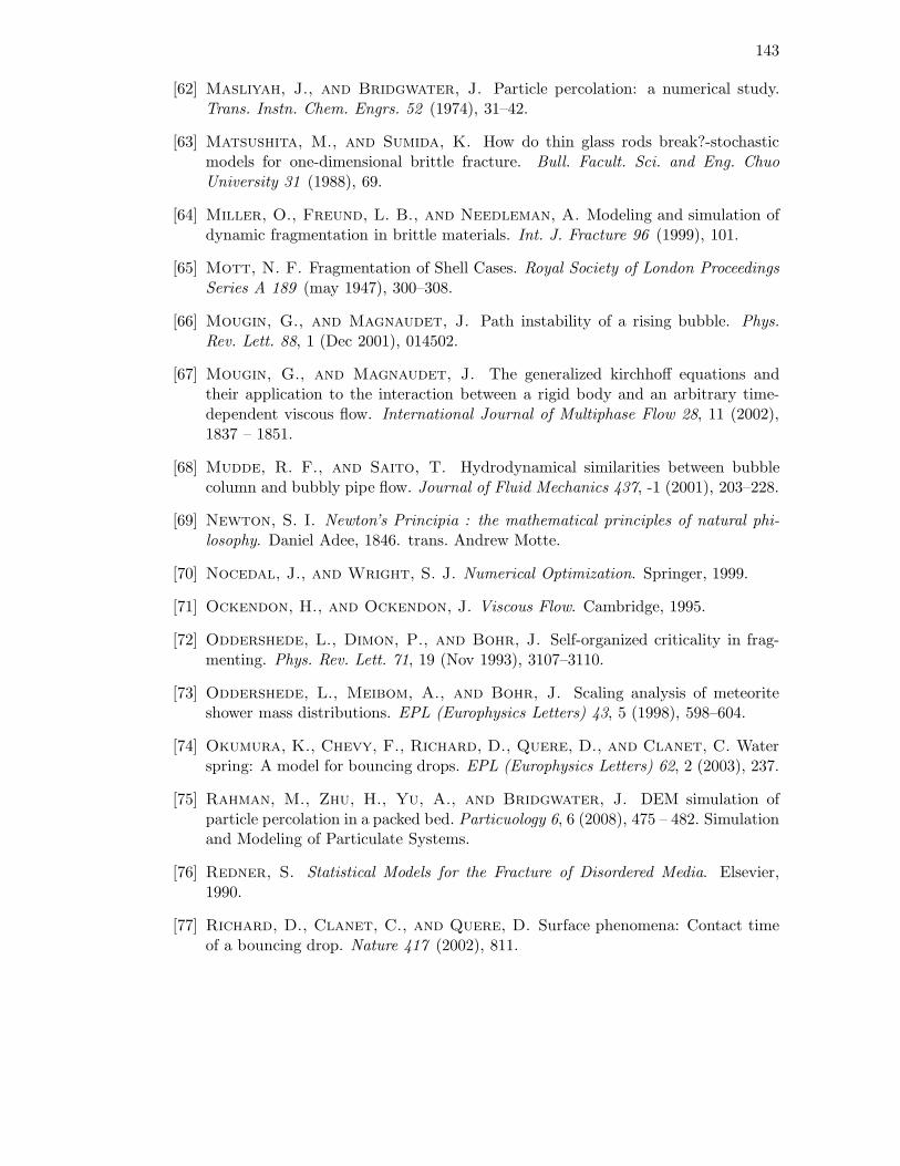
143
[62] Masliyah, J., and Bridgwater, J. Particle percolation: a numerical study.Trans. Instn. Chem. Engrs. 52 (1974), 31–42.
[63] Matsushita, M., and Sumida, K. How do thin glass rods break?-stochasticmodels for one-dimensional brittle fracture. Bull. Facult. Sci. and Eng. ChuoUniversity 31 (1988), 69.
[64] Miller, O., Freund, L. B., and Needleman, A. Modeling and simulation ofdynamic fragmentation in brittle materials. Int. J. Fracture 96 (1999), 101.
[65] Mott, N. F. Fragmentation of Shell Cases. Royal Society of London ProceedingsSeries A 189 (may 1947), 300–308.
[66] Mougin, G., and Magnaudet, J. Path instability of a rising bubble. Phys.Rev. Lett. 88, 1 (Dec 2001), 014502.
[67] Mougin, G., and Magnaudet, J. The generalized kirchhoff equations andtheir application to the interaction between a rigid body and an arbitrary time-dependent viscous flow. International Journal of Multiphase Flow 28, 11 (2002),1837 – 1851.
[68] Mudde, R. F., and Saito, T. Hydrodynamical similarities between bubblecolumn and bubbly pipe flow. Journal of Fluid Mechanics 437, -1 (2001), 203–228.
[69] Newton, S. I. Newton’s Principia : the mathematical principles of natural phi-losophy. Daniel Adee, 1846. trans. Andrew Motte.
[70] Nocedal, J., and Wright, S. J. Numerical Optimization. Springer, 1999.
[71] Ockendon, H., and Ockendon, J. Viscous Flow. Cambridge, 1995.
[72] Oddershede, L., Dimon, P., and Bohr, J. Self-organized criticality in frag-menting. Phys. Rev. Lett. 71, 19 (Nov 1993), 3107–3110.
[73] Oddershede, L., Meibom, A., and Bohr, J. Scaling analysis of meteoriteshower mass distributions. EPL (Europhysics Letters) 43, 5 (1998), 598–604.
[74] Okumura, K., Chevy, F., Richard, D., Quere, D., and Clanet, C. Waterspring: A model for bouncing drops. EPL (Europhysics Letters) 62, 2 (2003), 237.
[75] Rahman, M., Zhu, H., Yu, A., and Bridgwater, J. DEM simulation ofparticle percolation in a packed bed. Particuology 6, 6 (2008), 475 – 482. Simulationand Modeling of Particulate Systems.
[76] Redner, S. Statistical Models for the Fracture of Disordered Media. Elsevier,1990.
[77] Richard, D., Clanet, C., and Quere, D. Surface phenomena: Contact timeof a bouncing drop. Nature 417 (2002), 811.

144
[78] Richard, D., and Quere, D. Bouncing water drops. EPL (Europhysics Letters)50, 6 (2000), 769.
[79] Rosato, A., Blackmore, D., Buckley, L., Oshman, C., and Johnson, M.
Experimental, simulation and nonlinear dynamics of galtons board. Int. J. Nonlin.Sci. Num. Simul. 5 (2004), 289–312.
[80] Ross, S. M. Stochastic Processes. Wiley and Sons, 1983.
[81] Samson, L., Ippolito, I., Batrouni, G. G., and Lemaitre, J. Diffusiveproperties of motion on a bumpy plane. European Physical Journal B 3 (jul 1998),377–385.
[82] Schilling, M. F. The longest run of heads. The College Mathematics Journal21 (1990), 196 – 207.
[83] Serayssol, J.-M., and Davis, R. H. The influence of surface interactions onthe elastohydrodynamic collision of two spheres. Journal of Colloid and InterfaceScience 114, 1 (1986), 54 – 66.
[84] Shorlin, K. A., de Bruyn, J. R., Graham, M., and Morris, S. W. Devel-opment and geometry of isotropic and directional shrinkage-crack patterns. Phys.Rev. E 61, 6 (Jun 2000), 6950–6957.
[85] Sone, D., Sakakibara, K., Yamada, M., Sanada, T., and Saito, T. Bubblemotion and its surrounding liquid motion through the collision of a pair of bubbles.Journal of Power and Energy Systems 2, 1 (2008), 306–317.
[86] Sotolongo-Costa, O., Moreno-Vega, Y., Lloveras-Gonzalez, J. J., and
Antoranz, J. C. Criticality in droplet fragmentation. Phys. Rev. Lett. 76, 1 (Jan1996), 42–45.
[87] Stevin, S. The Principal Works of Simon Stevin, Mechanics, Vol. I. Swets &Zeitlinger, 1955. Dijksterhuis, E.J. (eds), made available by the Royal NetherlandsAcademy of Arts and Sciences.
[88] Stocchino, A., and Guala, M. Particle-wall collision in shear thinning fluids.Experiments in Fluids 38 (2005), 476–484.
[89] Stoer, J., and Bulirsch, R. Introduction to Numerical Analysis, third edi-tion ed. Springer, 2002.
[90] Stoppard, T. Rosencrantz and Guildenstern Are Dead. Grove Press, 1967.
[91] Stronge, W. J. Impact Mechanics. Cambridge University Press, 2000.
[92] Tsao, H.-K., and Koch, D. L. Collisions of slightly deformable, high reynoldsnumber bubbles with short-range repulsive forces. Physics of Fluids 6, 8 (1994),2591–2605.

145
[93] Tsao, H.-K., and Koch, D. L. Observations of high reynolds number bubblesinteracting with a rigid wall. Physics of Fluids 9, 1 (1997), 44–56.
[94] Tversky, A., and Kahneman, D. Belief in the law of small numbers. Psycho-logical Bulletin 76 (1971), 105.
[95] Wells, J. C. Mathematical modelling of normal collision of smooth elastic spheresin liquid. In Powders and Grains 93 (1993), C. Thornton, Ed., Association for theStudy of Granular Media, A. A. Balkema / Rotterdam / Brookfield, pp. 45–50.
[96] Wilkinson, D. R., and Edwards, S. F. Spontaneous interparticle percolation.Proceedings of the Royal Society of London. Series A, Mathematical and PhysicalSciences 381, 1780 (1982), 33–51.
[97] Wu, M., and Gharib, M. Experimental studies on the shape and path of smallair bubbles rising in clean water. Physics of Fluids 14, 7 (2002), L49–L52.
[98] Yang, F. L., and Hunt, M. L. Dynamics of particle-particle collisions in aviscous liquid. Physics of Fluids 18 (2006), 121506.
[99] Yang, F.-L., and Hunt, M. L. A mixed contact model for an immersed collisionbetween two solid surfaces. Philosophical Transactions of the Royal Society A:Mathematical, Physical and Engineering Sciences 366, 1873 (2008), 2205–2218.
[100] Zenit, R., Koch, D. L., and Sangani, A. S. Measurements of the averageproperties of a suspension of bubbles rising in a vertical channel. Journal of FluidMechanics 429, -1 (2001), 307–342.
[101] Zenit, R., and Legendre, D. The coefficient of restitution for air bubblescolliding against solid walls in viscous liquids. Physics of Fluids 21, 8 (2009),083306.

Vita
Michael Higley
Education
The Pennsylvania State University State College, PA 2003–2010
Ph.D. in Mathematics, expected in May 2010
Brigham Young University Provo, UT 1998–2000
M.S. in Mathematics
Brigham Young University Provo, UT 1992–1998
B.S. in Mathematics
Recognitions and Scholarships
Teaching With Technology Certificate 2009Charles H. Hoover Memorial Award 2009Penn State Department of Mathematics Graduate Teaching Associate Status 2009Penn State Department of Mathematics Graduate Student Teaching Award 2008VIGRE Fellowship 2003-2008Summer Industrial Internship Program (PSU Math Dept.) at Generation5, Toronto 2005
Research Experience
Doctoral Research The Pennsylvania State University 2005–2009Thesis Advisor: Prof. Andrew BelmonteExperimental, numerical and theoretical work in the W. G. Pritchard Laboratories inthe Mathematics Department at Penn State.
Teaching Experience
Graduate Teaching Assistant The Pennsylvania State University 2003–2009
Primary instructor for sections ranging from basic Algebra toVector Calculus and Differential Equations.
Graduate Teaching Assistant Brigham Young University 1998-2000
Primary instructor for sections of Algebra, lab instructor for Calculus.