Stigma and Social Control

Lawrence Blume

119

Reihe Ökonomie

Economics Series

119

Reihe Ökonomie

Economics Series

Stigma and Social Control

Lawrence Blume

July 2002

Institut für Höhere Studien (IHS), Wien Institute for Advanced Studies, Vienna

Contact: Lawrence Blume Department of Economics Uris Hall Cornell University Ithaca, New York 14850, USA email: lb19@cornell.edu

Founded in 1963 by two prominent Austrians living in exile – the sociologist Paul F. Lazarsfeld and the economist Oskar Morgenstern – with the financial support from the Ford Foundation, the Austrian Federal Ministry of Education and the City of Vienna, the Institute for Advanced Studies (IHS) is the first institution for postgraduate education and research in economics and the social sciences in Austria. The Economics Series presents research done at the Department of Economics and Finance and

aims to share “work in progress” in a timely way before formal publication. As usual, authors bear full responsibility for the content of their contributions. Das Institut für Höhere Studien (IHS) wurde im Jahr 1963 von zwei prominenten Exilösterreichern –dem Soziologen Paul F. Lazarsfeld und dem Ökonomen Oskar Morgenstern – mit Hilfe der Ford-Stiftung, des Österreichischen Bundesministeriums für Unterricht und der Stadt Wien gegründet und ist somit die erste nachuniversitäre Lehr- und Forschungsstätte für die Sozial- und Wirtschafts -

wissenschaften in Österreich. Die Reihe Ökonomie bietet Einblick in die Forschungsarbeit der Abteilung für Ökonomie und Finanzwirtschaft und verfolgt das Ziel, abteilungsinterne Diskussionsbeiträge einer breiteren fachinternen Öffentlichkeit zugänglich zu machen. Die inhaltliche Verantwortung für die veröffentlichten Beiträge liegt bei den Autoren und Autorinnen.

Abstract

Social interactions provide a set of incentives for regulating individual behavior. Chief among

these is stigma, the status loss and discrimination that results from the display of stigmatized

attributes or behaviors. The stigmatization of behavior is the enforcement mechanism behind

social norms. This paper models the incentive effects of stigmatization in the context of

undertaking criminal acts. Stigma is a flow cost of uncertain duration which varies negatively

with the number of stigmatized individuals. Criminal opportunities arrive randomly and an

equilibrium model describes the conditions under which each individual chooses the

behavior that, if detected, is stigmatized. The comparative static analysis of stigma costs

differs from that of conventional penalties. One surprising result with important policy

implications is that stigma costs of long duration will lead to increased crime rates.

Keywords Crime, stigma, social norms

JEL Classifications C730, Z130

Comments I am grateful to the Cowles Foundation for Economic Research, the Department of Economics at Yale

University, and the Institute for Advanced Studies in Vienna for very productive visits. I am also grateful for financial support from the John D. and Catherine T. MacArthur Foundation, the Pew Charitable Trusts, and the National Science Foundation. This research is a consequence of several stimulating conversations with Daniel Nagin, and has been helped along by comments from Buz Brock, Tim Conley, Steven Durlauf, Tim Fedderson, Josef Hofbauer, Karla Hoff, Chuck Manski, and Debraj Ray.

Contents

1 Introduction 1

2 The Model 3

3 Individual Choice and Social Equilibrium 5 3.1 States and Strategies ...............................................................................................5

3.2 The Individual’s Decision Problem .............................................................................6

3.3 Equilibrium – Existence and Monotone Comparative Statics .........................................8

3.4 A Discrete Example ...............................................................................................10

4 The Equilibrium Tagging Process 12 4.1 Birth and Death Rates ...........................................................................................13

4.2 Equilibrium in the Long Run ....................................................................................13

4.3 Tag Duration in the Long Run .................................................................................15

4.4 The Discrete Example: Short Run, Large N ..............................................................16

4.5 The Discrete Example: Long Run, Large N ...............................................................17

5 Conclusion 19

6 Proofs 23 6.1 Theorems 1, 2 and 3 .............................................................................................23

6.2 Theorem 4 ...........................................................................................................32

6.3 Computing Equilibria .............................................................................................33

Notes 34

References 36

Introduction 1

“. . . , let her cover the mark as she will, the pang of it will bealways in her heart.”

The Scarlet LetterNathaniel Hawthorne

1 Introduction

Consciously or not, in our interactions with others we identify markers thatsignal particular attributes. While the attribution signalled by a markermay be the result of rational inference, markers may also signal attributes bytriggering stereotypes. Language usage, skin color, gender and occupationmay all prompt individuals to infer that others possess a variety of behaviorsand attitudes that have nothing at all to do with the markers they display.Markers that trigger negative stereotypes stigmatize their bearers.

The sociology and social psychology literature on stigma is repletewith characterizations of the stigmatic process. Link and Phelan’s (2001,p. 367) definition is particularly useful here because it addresses the socialas well as the psychological aspects of stigma. They characterize stigma interms of four interrelated components:

In the first component, people distinguish and label human dif-ferences. In the second, dominant cultural beliefs link labeledpersons to undesirable characteristics—to negative stereotypes.In the third, labeled persons are placed in distinct categories soas to accomplish some degree of separation of “us” from “them”.In the forth, labeled persons experience status loss and discrimi-nation that leads to unequal outcomes.

Stigma has both micro- and macrosocial consequences. Link and Phelan(2001) assert that research on stigma has attended primarily to its perceptionby individuals and its consequences for micro-level interactions. On the otherhand, stigmatic markers classify entire groups of individuals. The aggregateof behaviors which respond to stigmatic markers has systemic implicationsfor aggregate social and economic performance.

Introduction 2

Both individual characteristics and individual behaviors are availablefor stigmatic representation. The stigmatization of race, gender, physicaldisabilities, mental illness and other characteristics is morally repugnant, anda continuing source of social ills. But the stigmatization of behaviors is thecentral mechanism for enforcing social norms. Stigma is thus essential to theproduction of what some call “social capital”. Stigma enforces social normsby stigmatizing non-normative behavior. Here this mechanism is modeledin order to draw some conclusions about its efficacy. A concrete instance ofthe social control process modeled here is the stigmatization of certain kindsof criminals. Small-town newspapers routinely publish the names of thosearrested (and not yet convicted) for driving under the influence of alcohol.Fears of public exposure are a strong incentive for tax compliance in somecommunities. But if everyone cheated or everyone drank, the social costs ofexposure would be small.1

The stigma mechanism suggests a coordination game, with high- andlow-activity equilibria. In the high-activity equilibrium, many people cheat,and so the stigma costs of cheating are small — cheating is not stigmatized.The low-activity equilibria has few cheaters and high stigma costs — cheatersare stigmatized. But my interest here is in the dynamics of stigma costsrather than in the description of static coordination games. The costs ofbeing stigmatized are born in the future as well as today. Accounting for thefuture requires the consideration of stigma cost dynamics.

The model presented here is a dynamic population game model, loose-ly in the spirit of Blume (1993), Kandori, Mailath, and Rob (1993) and Young(1993). But it departs from these earlier dynamic models in its rejection ofmyopia. The usual population model from evolutionary game theory su-perimposes on a static game some dynamics meant to describe the flow ofthe distribution of strategies among the population. The chief drawback tothis conventional modelling strategy is that individuals’ decisions are uncon-nected to considerations of the future. This is frequently justified by claimingthat individuals are myopic. With infinite subjective rates of time preferencethey have no need to consider the future consequences of their acts. Thetechnical innovation of this paper is developing a population model in whichindividuals care about the future and account for the future evolution of thepopulation in their decisionmaking. A suitable equilibrium concept is intro-duced and proved to exist. The comparative dynamics of equilibrium with

The Model 3

respect to parameters of the model is worked out. The long-run implica-tions for levels of criminal activity are demonstrated. Finally, a particularexample is worked out in some detail, which demonstrates some additionalconsequences of equilibrium both in the short and in the long run.

2 The Model

Consider the criminal story — the stigmatization of tax cheaters and drunkdrivers. The model contains two types of individuals: “Tagged” individualshave been caught and labeled as criminals at some point in the past. Theyhave been stigmatized by having been caught displaying antisocial behav-ior. “Untagged” individuals bear no such label. There is a cost associatedwith criminal status. The magnitude of this cost is increasing in the size ofthe untagged population. There is no further stigma cost to additional crimeonce an individual is tagged. Tagged individuals revert to untagged status atrandom moments. The stigma of being tagged eventually wears off. This dis-tinguishes crime, occupational choice and other stigmata marked by actionsfrom those marked by characteristic, such as race, gender and mental illness,which may never wear off. Time is continuous and individuals maximize thepresent discounted value of a utility stream whose magnitude depends uponthe following parameters.

Notation:

N The population size.

mt The fraction of “other” untagged individuals.

p The arrival rate of criminal opportunities.

u The (random) utility reward for successfully completing a crime.

v The utility penalty for being apprehended and convicted. δ = u − qv isthe expected instantaneous return to committing a crime.

F (u) The cdf of the reward u.

The Model 4

q The probability of being captured and convicted after committing a crime.(We suppose the corresponding probability conditional on not commit-ting a crime is 0.)

c(m) The stigma (flow) cost of being tagged when the fraction of others whoare untagged is m. This function is non-decreasing.

g The arrival rate of untaggings.

r The individual’s instantaneous rate of time preference.

Intuitively, the equilibrium process evolves as follows. At randommoments events happen to individuals in the population. Events are eithercrime opportunities or the removal of a tag (if present). Crime opportunitiesarrive to a given individual at rate p. When a crime opportunity arrives areturn u to committing the criminal act is drawn (independently) from thedistribution F . The individual, knowing the state and the return to crime,must decide whether or not to act. If she does not act, she receives 0 returnand is not tagged. If she commits the crime and is not caught she gets thereward u and remains untagged. This happens with probability 1 − q. Butwith the complementary probability q she is caught, pays a penalty v, andis tagged. Opportunities to become untagged arrive to a given individualat rate g. If she is not tagged, nothing happens, but if she is tagged, shebecomes untagged.

These processes are independent across individuals. Given decisionrules for the other individuals and the arrival rates of events described above,the process mt

∞t=0 describing the evolution of states for individual i’s deci-

sion process can be constructed.2

Individuals have beliefs about the state process. At a criminal op-portunity, they act so as to maximize the expected present discounted valueof their utility stream. An equilibrium tag process is the tag process whichresults when individuals’ beliefs are correct.

Choice and Equilibrium 5

3 Individual Choice and Social Equilibrium

The goal of this section is to define formally the tag process and the equi-librium concept just described. We will prove that there exists a uniquesymmetric equilibrium in state-dependent strategies. This equilibrium willbe monotone in the sense that the probability of an untagged individualcommitting a crime is increasing in the state. Furthermore, the equilibriumstrategies will involve randomization in at most one state.

This paper is concerned only with symmetric equilibria, in which allindividuals adopt the same strategy, which depends only upon the state.Our definitions will be phrased accordingly, although generalizations of thedefinition (not the theorems) are obvious.

3.1 States and Strategies

At a criminal opportunity, each individual’s decision will depend upon theimmediate value of the crime and the state of everyone else. That state is anelement of the decision maker’s state space Ω = 0, 1/(N − 1), . . . , 1, withtypical element m. Denote by m+ the state m + 1/(N − 1), and by m− thestate m − 1/(N − 1).

At any moment of time, an individual can be in one of two conditionsor types, untagged or tagged. A pure strategy for an individual currently oftype d = U, T (untagged, tagged) is a map which assigns to each statem and each immediate reward u a probability of committing the crime.Formally, a pure strategy for an individual currently of type d ∈ U, T(untagged, tagged) is a map

σd : Ω × R → Commit, Not.

A (behavior) strategy for each type d = U, T (untagged, tagged) is a map

σd : Ω × R → [0, 1],

where σd(m, u) is the probability that a type d individual commits a crimewith reward u in population state m. A strategy is a pair of type strategies

Choice and Equilibrium 6

σ = (σU , σT ). A strategy is monotonic if, for each type, the probability ofcommitting a crime falls with the state. That is, the greater the fractionof untagged individuals, the lower the probability of anyone’s committinga crime. A reservation strategy exhibits a return threshold u∗ above whichcrimes are committed and below which they are not.

Definition 1. A strategy σ is monotonic if for all d and u, σd(m, u) is non-decreasing in m. It is a reservation strategy if for all d and m there is a u∗

such that σd(m, u) = 1 for u > u∗ and σd(m, u) is 0 for u < u∗.

At any instant of time at most one individual has an opportunityof some kind, and so the value of the state process can change by at most±1/(N −1). Consequently the state process mtt≥0 is a birth-death process.The birth and death rates are determined by the (mixed) strategy σ. Sup-pose the population state is m. A “birth” occurs when a tagged individualbecomes untagged. The rate at which opportunities arrive to tagged individ-uals is (N − 1)(1 − m), and the probability that an event is an untagging isg, so the birth rate is

λm = (N − 1)(1 − m)g (1)

A death occurs when an untagged individual commits a crime and is caught.The death rate for individual i’s state process depends upon her type. Definefor each type d and state m σd(m) =

∫

σd(m, u)dF (u) to be the probabilitythat a decisionmaker of type d will commit a crime in state m. We abusenotation by using this σ this way because it will be clear both from thecontext and by the number of arguments whether or not we want to conditionon the return. Suppose she is untagged and the state is m. Any otheruntagged individual also sees state m, and so the death rate is

µUm = (N − 1)mpσU (m)q (2)

If individual i is tagged and is in state m, then any other untagged individualsees state m+. in this case the death rate in state m is

µTm = (N − 1)m+pσU (m+)q

3.2 The Individual’s Decision Problem

When a criminal opportunity arrives, the individual who has received it mustdecide whether or not to commit a crime. The rational decisionmaker must

Choice and Equilibrium 7

account for the immediate expected return to a crime, and also for the streamof stigma costs. If the individual were fully rational and alert to all strategicinteractions, then in computing the expected present discounted value of thestigma cost of a crime she would account for the effect of her own tagging onthe propensity of others to commit crimes. When computing the evolution ofstates, she would assume death rates µT conditional on her being tagged, andµU conditional on her being untagged. We will assume that individuals areless strategic than this. They account for both instantaneous and dynamiceffects, but they neglect the incentive effect of their own decisions on others.Whether tagged or not, they they assume the state process has the samedeath rates µ = µU .3

The individual’s decision problem can be formulated as a dynamicprogram. The program is described by three independent processes: Thearrival process for criminal opportunities, the arrival process for untaggings,and the state process. The criminal opportunity process is a rate-p Poissonprocess and the untagging process is a rate-g Poisson process. The stateprocess has the birth and death rates λm and µm just described. All theserates can be derived from the parameters and σ, the strategy employed byothers. Thus given the parameters, each individual’s decision problem ischaracterized by (σT , σU).

At a decision opportunity the individual knows the history of the tagprocess, her individual history, and the payoff u to the current crime . Shechooses an action, to commit a crime or not, so as to maximize the expectedpresent value of her utility stream. Her instantaneous utility depends uponthe state of the population process, her current type, and whether or not shehas a decision opportunity.

At a moment which is not a decision opportunity she is either taggedor untagged. If untagged, her instantaneous utility is 0. If tagged, it is−c(mt). At a decision opportunity she is either tagged or untagged. Shedecides whether or not to commit a crime. If she chooses not to commit acrime, her instantaneous utility is that which she would receive were she notto have a decision opportunity. If she commits a crime, her utility dependsupon whether or not she is caught, and whether or not she is tagged. If sheis already tagged, she receives reward u. She pays a penalty v if caught, soher net return if caught is u−v. She has an instantaneous stigma cost flow of

Choice and Equilibrium 8

c(mt) which is independent of her decision and whether or not she is caught.

If she is untagged, she has the same immediate net reward structure:u for the crime, less a penalty v if she is caught. But if she is caught herstatus switches from untagged to tagged, and so she begins to pay the stigmacost flow c(mt) which she did not bear previously. This flow lasts a randomamount of time, independent of her future decisions, until the tag disappears.

Consider a sample path from the meet of the three processes and astrategy. The strategy generates a stream of utility. The value of the strategyon that path is the present discounted value of the utility stream (discountedat rate r), and the expected value of a strategy is the expectation of this valueover all sample paths of the meet. An optimal strategy maximizes expectedvalue over all strategies.

3.3 Equilibrium — Existence and Monotone Compar-

ative Statics

We will be looking for symmetric equilibria; that is, equilibria in which allindividuals use the same strategy. We can already see this in the constructionof the individual decision problem. In principle the definition of the problemcan be extended to encompass different individuals using different strategies.At that point, however, the birth-death formalism is lost because in order tokeep track of the evolution of mt we would need to know the identities of thetagged individuals.

Definition 2. A strategy σ = (σU , σT ) is a population equilibrium strategyprofile if σ is optimal for the individual decision problem with parameters σ.

This equilibrium is not Nash! It fails to be Nash because, as we discussedearlier, each individual neglects the impact of her policy on the evolution ofother individuals’ decisions. Nonetheless, this equilibrium concept is closeto Nash, and in some appropriate large-numbers limit it would be Nash. Tothe extent that equilibrium fails to be Nash, it is a consequence of a smallnumbers problem.

Choice and Equilibrium 9

It would seem that somehow a strategic complementarity must ex-ist. As more people commit crimes, more people become tagged and theexpected stigma cost of committing a crime falls, making crime more at-tractive. However, at this point we cannot even define a meaningful notionof strategic complementarity since there is no natural order for the strategyspace with respect to which there might be increasing differences and thelike. Nonetheless we will see that the strategic complementarity intuition isessentially correct.

The first Theorem describes population equilibria:

Theorem 1. A population equilibrium exists, every population equilibriumuses monotonic reservation strategies and is pure in all but at most one state,and σT (m, u) is 1 if δ > 0 and 0 if δ < 0.

Existence is not a surprise. It is also not surprising that if crime does not payin the short run, it never pays. Monotonicity for δ > 0 is a consequence ofthe birth-death construction and the monotonicity of instantaneous rewardswith respect to the state mt. It is not hard to see that for an open and denseset of parameter values, equilibrium is pure. The case δ = 0 is just like δ > 0for all states except m = 0, where anything can be chosen.

It will prove useful to track the states at which, for a given utilitylevel, crime begins to take place with positive probability.

Definition 3. Let σ denote an equilibrium strategy. For each utility level u,let

mu = max

m : σU (m, u) > 0 ∪ +∞

.

The state mu is the switch point for u in strategy σ.

The presence of strategic complementarities has implications for thedependence of equilibrium on model parameters. Say that strategy σ is “ascriminal as” strategy σ′ if, in every event and for every type and payoff, theprobability of committing a crime under σ is at least that under σ ′.

Definition 4. Strategy σ is at least as criminal as strategy σ ′ (write σ σ′)iff for each state m, type d and payoff u, σd(m, u) ≥ σd(m

′, u).

Choice and Equilibrium 10

Real-valued parameters are ordered in the usual way. Payoff distributionsare ordered by means. That is, F ≥m G iff the mean of F is at least as bigas the mean of G. Cost functions are ordered pointwise. c( · ) ≥ d( · ) if forall m, c(m) ≥ d(m). With respect to these orderings and the “at least ascriminal as” ordering there is a comparative equilibrium result.

Theorem 2. For each vector of parameter values the set of equilibria aretotally ordered by , and there is a greatest and a least equilibria. Theseextreme equilibria are increasingly criminal in F and r, and decreasinglycriminal in c and v.

The effects of changes in g and q are ambiguous, and will be discussed furtherbelow.

3.4 A Discrete Example

The simplest examples to compute have a distribution of utilities with twopossible values: One such that the crime never pays and one such that crimesometimes pays. Suppose that a cost function is defined on the interval[0, 1]. It is non-decreasing and piecewise-continuous. There are two possiblereward values: uh, realized with probability ε > 0, very small, which is sohigh that any such criminal opportunity is always acted upon, and ul whichmay or may not be acted upon by untagged individuals, depending upon theexpected present discounted value of stigma costs.

Equilibrium is characterized by the switch point s, the largest state inwhich a crime with reward ul will be carried out by an untagged individual,and ps, the probability of carrying out a crime in state s. For all states lessthan s, the probability of committing a crime with reward ul is 1, and ps

will be 1 as well, unless the individual is indifferent between committing thecrime and abstaining.

Equilibria in this model are easily computed by methods discussed insection 6. This makes possible an investigation of the comparative statics ofchanges in parameters g and q which were not determined by complementar-ity arguments.

Choice and Equilibrium 11

The effects of changes in g and q are ambiguous. On the one hand,increasing q increases the probability of being caught and paying direct andstigma costs. As in Becker’s (1968) model of criminal deterrence, this neoclas-sical effect reduces criminal activity. But a second consequence of increasingq is a social interaction effect. Increasing q increases the number of taggedindividuals, thereby reducing the stigma costs of having been caught com-mitting a crime. This effect increases criminal activity. The comparativestatics of a change in q depends upon the balance between these two effects.A downward sloping relationship between the probability of getting caughtq and criminal activity is easily illustrated in simple examples.

In the following example, v = 0 to focus on stigma costs. A sliceof the equilibrium correspondence, plotting the relation between equilibriums and q.4 Every dot indicates an equilibrium switchpoint. This example

0.4

0.42

0.44

0.46

0.48

0.5

0.52

0.54

0.56

0.4 0.5 0.6 0.7 0.8 0.9 1q

s

Figure 1: The Equilibrium Correspondence: s vs. q.

illustrates nicely the possibility of multiple equilibria. The example exhibitsthe neoclassical relationship between the probability of getting caught andthe criminality of the equilibrium strategy over most of its range. But for qlarge enough, the social interaction effect dominates. The comparative staticschanges direction; increasing q increases the criminality of the equilibriumstrategy set.

Not surprisingly, similar effects are at work in the relationship be-tween equilibria and the parameter g, the arrival rate of untaggings. When

Dynamics 12

g increases, the conventional effect is that stigmatic markers are held for ashorter period of time, and so stigma costs decrease. Hence criminal activ-ity should become more likely. The social interaction effect, however, has itthat fewer individuals are tagged at any moment in time, and so the flowcosts of stigma have increased. The social interaction effect dominates inthe downward-sloping part of the following figure.5 Expected duration of the

0.3

0.35

0.4

0.45

0.5

0.55

0.6

0.65

0 0.1 0.2 0.3 0.4 0.5 0.6

s

g

Figure 2: The Equilibrium Correspondence: s vs. g.

stigmatic punishment, 1/g, is in fact a policy variable of those courts whichadminister so-called “shaming-penalties”.6 Book (1999) relates that in colo-nial Williamsburg a convicted thief was nailed by his ear to the pillory. Atthe completion of his sentence his gaolers ripped him from the pillory withoutfirst removing the nail, thereby “earmarking” him for life. That is, g = 0.Overly long punishments can have the perverse effect of reducing the incen-tives to avoid criminal activity. The positive effect on the cost of increasingthe waiting time τ is more than offset by the decreases in cost created bychanges in the mtt≥0 process.

4 The Equilibrium Tagging Process

The ebb and flow of criminal behavior, long run averages and likely shortrun paths, are properties of the population tag process. This process is de-

Dynamics 13

rived from the equilibrium strategy and the assumptions about the stochasticprocesses generating crime opportunities, capture, and untagging.

4.1 Birth and Death Rates

Define the population state space S = 0, 1/N, . . . , 1. Let ntt≥0 denotethe population process for a population of size N . This is a birth-deathprocess with birth rates κN

n and death rates νNn :

κNn = N(1 − n)g

νNn = NnpσU

(Nn − 1

N − 1

)

q

The argument of σU is computed as follows. In population state n, an un-tagged individual sees Nn − 1 other untagged individuals, so the fraction ofothers who are tagged is m(n) = (Nn − 1)/N . These birth and death ratescompletely characterize the population process, including its short run andlong run behavior. Let n+ and n− denote the next biggest and next smalleststates to n, n + (1/N) and n − (1/N), respectively.

4.2 Equilibrium in the Long Run

For any equilibrium, the long run behavior of the population process is de-scribed by its invariant distribution. The state process is always ergodic.Since the birth rate is strictly positive for any n > 0, it is possible to reach 1from any state. Consequently the state process has a unique invariant distri-bution. For instance, if there is a state m∗ such that no crimes are committedfor m > m∗, then the unique invariant distribution puts all its mass on thestate n = 1.

One virtue of the birth-death formalism is that the invariant distri-bution is easily computed. The invariant distribution π is characterized bythe relationship

π(n)κNn = π(n+)νN

n+

Dynamics 14

Iterating this relationship, we have that if there is a state n′ such that νNn′ = 0,

then π(n) = 0 for all n < n′, and if n′ = maxn : νNn = 0, then for all n > n′,

π(n)

π(n′)=

n−

∏

k=n′

κNk

νNn+

=n−

∏

k=n′

1 − k

k

g

pqσU

(

Nk−1N−1

) (3)

where the index is understood as being incremented in units of size 1/N .

The invariant distribution allows for the calculation of such variablesas the long run crime rate. If the population is in state n, the rate at whichindividuals commit crimes is

η(n) = N(1 − n)p + Nnpσ(Nn − 1

N − 1

)

;

The N(1 − n) tagged individuals commit crimes at rate p; every crime thatcomes their way. The Nn untagged individuals commit crimes at the lowerrate given by their strategy. The average of this function with respect to theinvariant distribution gives the long run crime rate.

The comparative equilibrium analysis of Theorem 2 has straightfor-ward implications for the long run behavior of the population state process.Let x be a parameter with respect to which equilibrium is increasing. As xincreases, the death rates in each state increase. The theorem states that ineach state m = (N − Nn)/(N − 1), the probability of committing a crimeis (weakly) increasing, and so, according to the definition, is the death rateνN

n . The birth rates are fixed by the parameter g, and so remain unchanged.Comparative static analysis of equilibrium strategies has straightforward im-plications for changes in death rates, and therefore for changes in the invari-ant distribution.

Theorem 3. The invariant distribution is non-increasing with respect toparameters F and r in the sense of first-order stochastic dominance, andnon-decreasing in c and v.

Corollary 1. The crime rate η(n) is non-decreasing with F and r, and non-increasing in c and v.

Dynamics 15

4.3 Tag Duration in the Long Run

The failure of the conventional intuition to predict the effects of changesin g and q on the criminality of equilibrium strategies depends upon thevalues of other parameters. Cases other than those presented in the previoussection present the predicted comparative statics. But the effects of theseparameters is due not just to the equilibrium strategies but also to the rateat which those committing crimes are tagged, and the rate at which they aresubsequently untagged. Due to this second effect, the counterintuitive effectof increasing g on the invariant distribution and on the long-run crime rateis universal for large enough parameter values.

Denote by σ∗ the map from Ω × R → Commit, Not such thatσ(ω, u) = Commit if and only if u − qv ≥ 0. Recall that regardless of pa-rameter values, σT = σ∗. Any strategy σU more criminal than σ∗ is stronglydominated by it, since the additional opportunities σU accepts that σ∗ doesnot have negative immediate rewards. More generally, if σd is any reservationstrategy which in some recurrent state ω has a threshold u < qv, it is strictlydominated by the strategy which raises the threshold in state ω to qv.

Let η∗ = p(

1−F (qv))

denote the crime rate which would be observedif all untagged individuals acted according to σ∗. From these considerationsthe following lemma is obvious.

Lemma 1. The long run equilibrium crime rate η(n) is bounded above by η∗.

We should expect this upper bound to be achieved for large values of g.When g is large, the expected duration of a tag is small, and status costsbecome negligible. The neoclassical effect should dominate the social inter-action effect. This is true, but the bound can also be achieved for small g.Intuitively, when g is sufficiently small, any tag lasts a very long time. Inthe long run, most of the population will be tagged most of the time, andtherefore most behavior is governed by σT = σ∗, rather than σU (whatever itmay be). Let µ0 denote the probability distribution on S which puts all itsmass on 0, and let µ1 denote point mass at 1.

Theorem 4. Suppose that F(

qv + qc(1)/r)

< 1. Then limg→0 µg = µ0.Suppose that F (u) is continuous at u = qv. Then limg→∞ µg = µ1. In bothcases, limg→0 η(n) = η∗.

Dynamics 16

If status costs ever have an impact on choice, then the long run crime ratemust be decreasing in g over some range of values.

4.4 The Discrete Example: Short Run, Large N

For any differentiable function f : S → R the birth and death rates givea differential equation which characterizes the evolution of the conditionalexpectation of f through time:

d

dτEf(nt+τ )|nt = n

∣

∣

τ=0= κN

n

(

f(n+) − f(n))

+ νNn

(

f(n−) − f(n))

= κNn f ′(n)

1

N− νN

n f ′(n)1

N+ O(N−2)

=(

(1 − n)g − npσU

(

m(n))

q)

f ′(n) + O(N−2)

If f(n) = n, then

d

dτEnt+τ |nt = n

∣

∣

τ=0= (1 − n)g − npσU

(

m(n))

q + O(N−2)

The differential equation

n = (1 − n)g − npσU

(

m(n))

q

is the mean field equation of the model. For the utility distributions consid-ered in this and the next section, it is of the form

n = (1 − n)g − npq(1 − ε) for n < s, (4a)

n = (1 − n)g − npqε for n > s, (4b)

with steady states

nl =g

g + pq(1 − ε)and nh =

g

g + pqε

(one for each branch), and solution

n(t) = nl +(

n(0) − nl

)

e−(

g+pq(1−ε))

t for n(0) < s, (5a)

Dynamics 17

n(t) = nh +(

n(0) − nh

)

e−(g+pqε)t for n(0) > s, (5b)

The mean field equation characterizes the behavior of the process overfinite time horizons in large populations. The following result is well-known inthe literature on density-dependent population processes (Ethier and Kurtz1986, Chapt. 10, Theorem 2.1).

Theorem 5. Let σN∞N=1 denote a sequence of equilibria in a population ofsize N , such that the switch points sN converge to a limit s. Suppose that n(t)is the solution to the differential equation (4) from initial condition n0 6= s,and let nN

t denote the random variable that describes the population state attime t in a population of size N beginning from initial condition nN(0) = n0.Then for all T > 0, limN→∞ supt≤T |nN

t − n(t)| = 0 a.s.

The steady states are states in which the rate at which untagged individualsare tagged just equals the rate at which tagged individuals are untagged.The two different steady states correspond to the different rates at whichuntagged individuals commit crimes above and below the switch point. Thisis not to say that the two steady states are realized in practice. If for instance,s > nh, then nh is actually in the regime of low criminal activity. Startingfrom a high state, nt will move downward according to equation (5a) untilstate s is reached, and then continue moving down through nh according toequation (5b).

4.5 The Discrete Example: Long Run, Large N

In the discrete model with ε > 0 the equilibrium odds ratios for an equilib-rium with switch point mu and no mixing are given by the following formulas.Let nu = mu + (1 − mu)/N .

π(n)

π(0)=

n−

∏

k=0

1 − k

k

g

pqσU

(

Nk−1N−1

)

=

(

N

Nn−

)(

g

pq(1 − ε)

)Nn−

if n− < nu,

(

N

Nn−

)(

g

pq(1 − ε)

)Nnu

(

g

pqε

)N(n−−nu)

if n− ≥ nu.

Dynamics 18

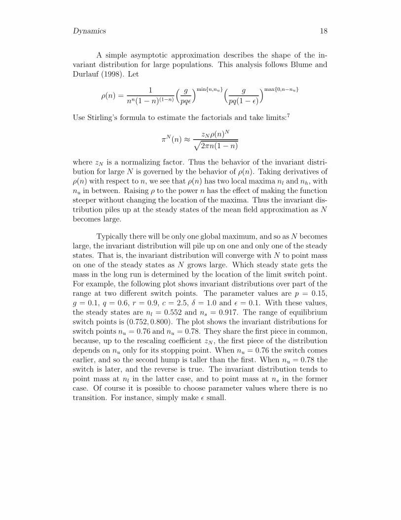
A simple asymptotic approximation describes the shape of the in-variant distribution for large populations. This analysis follows Blume andDurlauf (1998). Let

ρ(n) =1

nn(1 − n)(1−n)

( g

pqε

)minn,nu( g

pq(1 − ε)

)max0,n−nu

Use Stirling’s formula to estimate the factorials and take limits:7

πN(n) ≈zNρ(n)N

√

2πn(1 − n)

where zN is a normalizing factor. Thus the behavior of the invariant distri-bution for large N is governed by the behavior of ρ(n). Taking derivatives ofρ(n) with respect to n, we see that ρ(n) has two local maxima nl and nh, withnu in between. Raising ρ to the power n has the effect of making the functionsteeper without changing the location of the maxima. Thus the invariant dis-tribution piles up at the steady states of the mean field approximation as Nbecomes large.

Typically there will be only one global maximum, and so as N becomeslarge, the invariant distribution will pile up on one and only one of the steadystates. That is, the invariant distribution will converge with N to point masson one of the steady states as N grows large. Which steady state gets themass in the long run is determined by the location of the limit switch point.For example, the following plot shows invariant distributions over part of therange at two different switch points. The parameter values are p = 0.15,g = 0.1, q = 0.6, r = 0.9, c = 2.5, δ = 1.0 and ε = 0.1. With these values,the steady states are nl = 0.552 and ns = 0.917. The range of equilibriumswitch points is (0.752, 0.800). The plot shows the invariant distributions forswitch points nu = 0.76 and nu = 0.78. They share the first piece in common,because, up to the rescaling coefficient zN , the first piece of the distributiondepends on nu only for its stopping point. When nu = 0.76 the switch comesearlier, and so the second hump is taller than the first. When nu = 0.78 theswitch is later, and the reverse is true. The invariant distribution tends topoint mass at nl in the latter case, and to point mass at ns in the formercase. Of course it is possible to choose parameter values where there is notransition. For instance, simply make ε small.

Conclusion 19

0.5 0.55 0.6 0.65 0.7 0.75 0.8 0.85 0.9 0.95

ρ(n)

n

Figure 3: Invariant distributions for two different switch points.

5 Conclusion

A complete account of stigma as a social control process requires an analysisof how stigmatic attributions are formed. In fact there are many accounts.Closest to contemporary decision theory is a model of stereotyping whichrecognizes the use of overly simple models for categorization as an efficientallocation of cognitive resources.8 I offer no such account here. Instead I makemicro-level assumptions about the incentive effects of stigma. The drivingassumption of my analysis is that the cost of being stigmatized, however it isrealized, is low when many people bear the marker, and highest when only afew are so marked. Even this assumption would run afoul of some coherenttheories of stigmatization.9 To the extent that stereotyping is a statisticalphenomenon, it is hard to form stereotypes if the incidence of the marker islow. Here I envision the social control process runing on a time scale whichis short relative to the persistence of stereotypes, so that the stability of thestigmatic power of particular markers is not at issue. To the extent that thegroup at risk of stigmatization is large, the social cost of discipline may betoo high when a large fraction of the group is tagged. The social cost of

Conclusion 20

stigmatizing drunk drivers is small; the wage effects of a social custom notto hire those who park illegally could be enormous. Here I envision that thebehaviors being stigmatized are seriously considered by or feasible to a smallsubset of the total population.

The efficacy of the stigma as a social control mechanism raises thequestion of if, and how, it can be used as a policy tool. Lessig (1995) offers alovely anecdote about a government attempt to manipulate the stigma costfunction c. In the late 1950’s motorcycle helmets were beginning to leak fromwestern Europe into the Soviet Union, which produced none. For the Sovietleadership, the medical benefits of wearing helmets were exceeded by the so-cial cost of an invasion by a western style. “Thus began an extraordinaryand self-conscious campaign by the Soviet government to vilify the wearers ofmotorcycle helmets. Cartoons appeared in the popular (read: government-controlled) press, mocking the ‘white heads’ on cycles. By the early 1960s,people began wearing helmets only at night, to avoid easy detection.”10 Ac-cording to Lessig, helmets were never banned outright, suggesting that thestigmatization of riders was effective enough. Soon enough, however, the So-viets began to produce their own helmets, and with the availability of Soviethelmets, the campaign changed. Instead of stigmatizing helmet-wearers, itswitched to stigmatizing those who imported helmets. The stigma cost ofwearing helmets fell, and helmet usage increased.

Kahan (1997) claims a more subtle example of stigma manipulationin the policy of rewarding inner-city high school students who turn in peerscarrying guns. In his account, not carrying a gun is a stigmatic marker. Heargues that the reward policy succeeds because it manipulates stigma as wellas having a direct effect on the stock of guns. The stigmatic effect is thatwhen some students are out for the reward, displaying one’s gun becomesmore costly. If gun owners become more reluctant to display them, then themeaning of the marker changes, the stigma costs of not carrying falls, andthe incentive to carry a gun is reduced.

A third, prominant example of promoting social control through stig-ma management is the increased use of shaming punishments in the UnitedStates and Great Britain.11 In colonial America shaming could be for life. Inmodern times, shaming penalties are frequently seen as part of a probationsentence, a less costly and disruptive approach to behavior modification than

Conclusion 21

prison for appropriate convicts.

As a tool of social control, stigma can be mismanaged. Theorem 4shows that increasing the duration of stigma (decreasing g) will ultimatelyincrease the long run crime rate. The largest possible crime rates are achievedwhen the duration is extremely long. This point is not merely of academicinterest. Third strike drug offenders are banned for life from receiving avariety of federal benefits, including food stamps and temporary assistanceto needy families available under the Personal Responsibility and Work Op-portunity Reconciliation Act of 1996.12 In some states, businesses requiringlicenses cannot obtain them if they employ convicted felons, no matter howold the offense. This effective lifetime employment ban bars former convictsfrom working in, among other locations, barber shops and automobile bodyshops. In a similar vein, easy access to criminal records makes it easier foremployers not obligated by law to nonetheless turn down applicants withcriminal records. For instance, The Fair Credit Reporting Act prohibitedthe reporting of convictions more than seven years old, until this provisionwas deleted in 1998.13 This information be be socially useful for its signalvalue, but Theorem 4 suggests that the availability of such old informationmay well have a negative deterrent effect on crime.

Another important counter-productive effect of stigmatization is notcaptured in this model. When “normal” society shuns the stigmatized, somemay seek to shed the stigma (for instance, by having physical deformitiescorrected) or to overcome it by excelling in other dimensions. Others mayrespond by joining together with other stigmatized individuals to create“counter-communities” — communities in which the stigmatized activity isignored or even becomes a source of status.14 Newman (1999) writes aboutthe stigma teenagers attached to “flipping burgers” in Harlem and otherpoor New York neighborhoods and, in particular, about the strategies youngworkers employ to defend themselves against the jokes and ridicule directedat them.

. . . it is clear that the workplace itself is a major force in thecreation of a ‘rebuttal culture’ among these workers. Withoutthis haven of the fellow-stigmatized, it would be very hard forurger barn employees to retain their dignity. With this support,however, they are able to hold their heads up, not by definining

Conclusion 22

themselves as separate from society, but by callking upon theircommonality with the rest of the working world.15

Informal social control of deviance presumes a community which issufficiently cohesive, well-organized, and has sufficient resources to enforcesocial norms. Elijah Anderson’s (1990) ethnography of “Northton” describesthe how the clash between “decent” norms (family life, hard work, church-going) and “streetwise” norms (associated with crime and the drug culture)is facilitated by a weakened structural fabric. The negative correlation ofsocial organization and crime rates appears in empirical analyses as well.Sampson and Groves (1989) found in British data that neighborhoods withlower levels of social organization had higher levels of violent and propertycrimes. Unsupervised teen groups were the largest contributors to the violentcrime rate, while local friendship networks and organizational participationhad a large negative impact on robbery. Most surprisingly, the effect of themeasured indices of social organization on crime exceeded the direct effectsof socio-economic status. One source of disrupted friendship networks andbroken families is the high incarceration of young male African-Americans.The legislative response to the crack epidemic of the 80’s has been massivemandatory minumum sentences.16

A reinforcing effect of stigma not captured here is its effect on labellingthe boundaries of normative behavior. When Hester Prynne is marked withthe scarlet letter ‘A’, not only is she stigmatized, but the community reaffirmsfor itself the labelling of adulterous behavior as deviant. A contemporary(and perhaps non-fictional) instance of this labelling effect is the so-called“broken windows” theory which lies behind “order maintenance policing”.17

Lessig (1995), Kahan (1997) and others argue that the power of law to es-tablish social boundaries and create categories for stigmatization is not yetfully appreciated as a source of social control.

The account of stigma and the enforcement of social norms presentedhere extends the evolutionary game theory paradigm by offering a richeraccount of individual choice. In particular, forward looking behavior is rarelystudied, and almost never in stochastic models.18 Stigma is in essence adynamic phenomena. Its costs are born in the future, and the magnitudeof those costs are determined by the future actions of others. This is whythe pop rational actor social science accounts which, at their best, make

Proofs 23

reference to some kind of evolutionary game dynamics in a coordinationgame, seem so shallow. For instance, it would be hard to formulate a questionabout the effect of punishment duration in such models. The subject ofevolutionary game theory is the dynamics of player choice. Recognizingplayers as intertemporal decision makers models opens up a variety of newmodelling opportunities. Evolutionary game theory has been nearly devoidof serious applications to the social sciences. The premise of this paper isthat deeper models of individual choice will provide evolutionary game theorywith the wherewithal to address social issues.

6 Proofs

This section contains proofs of Theorems 1 through 4 and details on com-puting equilibria.

6.1 Theorems 1, 2 and 3

The proofs of Theorems 1 and 2 rely on the strategic complementarity thatworks through the stigma cost of crime. More criminal strategies lead tomore tagged individuals, which lowers the stigma costs, thereby making crimemore profitable. The complementarity appears twice in the proof: First toshow that the optimal response to any strategy is a monotonic reservationstrategy, and second to work the fixed point argument to get the existenceof equilibrium results and to sign the dependence of the equilibrium strategyset on parameters.

In the individual’s decision problem, states are the number of otherswho are tagged. The assumptions of the model implies that each individualtakes the state process to be a birth-death process with some given rates.States evolve, and independently, events happen. An event is the arrivalof either a criminal opportunity or an untagging. The event process is thesuperposition of two independent Poisson processes: A rate p process forcriminal opportunities and a rate g process for untaggings. The event processis a rate p + g Poisson process, and the probability that a given event is a

Proofs 24

criminal opportunity is p/(p+g). Types of events are uncorrelated over time.See Kingman (1993) for details.

Construction of value functions and evaluation of policies involvescomparing the values of functionals along paths of the state process. Thisis done with a coupling argument. Let ω denote a path of the birth-deathprocess mt

∞t=0, and define the function f(ω) =

∫ ∞

0e−λtg(ωt)dt on paths.

Lemma 2. If mt∞t=0 is a birth-death process and g(m) is non-decreasing in

m, Then Ef(ω)|ω0 = m is non-increasing in m. If g(m) is not constant,then the conditional expectation is strictly decreasing in m.

Proof. Choose m′ < m′′, and construct the stochastic process (xt, yt)∞t=0

with (x0, y0) = (m′, m′′) as follows: Let s = inft : xt ≥ yt denote thecoupling time of the xt and yt processes. Let xt evolve according to the birthand death rates of the mt-process. Let yt evolve according to the rates for themt-birth-death process, independently so long as xt < yt, that is, so long ast < s. Observe to that almost surely s < ∞ and that xs = ys. Let yt = xt fort ≥ s. Observe that each marginal process is a birth-death process evolvingaccording to the rates for the mt-process. Furthermore, almost surely xt ≤ yt

for all t.

Now consider the flows g(xt) and g(yt). Clearly g(xt) ≤ g(yt) almostsurely for all t. Consequently for almost all (xt, yt) paths,

∫ ∞

0

e−λtg(xt)dt ≤

∫ ∞

0

e−λtg(yt)dt

The expectation of the left hand side is Ef(ω)|ω0 = m′ and the expectationof the right hand side is Ef(ω)|ω0 = m′′, so the conditional expectationsare decreasing in m. If g(m) is not constant, there is a state m∗ such thatc(m) < c(n) for all m ≤ m∗ < n. For any (xt, yt) path such that for someinterval of time, xt ≤ m∗ < yt, the inequality is strict. The set of suchpaths has positive probability, and so the inequality between conditionalexpectations is strict.

The first application of this Lemma 2 compares the present discountedvalue of the flow cost of being tagged from one criminal opportunity to the

Proofs 25

next. An event is the arrival of either the next criminal opportunity orthenext untagging. The time to the next event, τ , is distributed exponentiallywith parameter p + g. Define

C(m) = Eτ,m

∫ τ

0

e−rtc(mt)dt∣

∣

∣m0 = m

= Em

∫ ∞

0

e−(r+p+g)tc(mt)dt∣

∣

∣m0 = m

To save space below, any expectation operator containing m in the subscriptwill denote an expectation conditional on the event m0 = m. Everythingto the right of the vertical line will be surpressed.

Lemma 3. C(m) is non-decreasing in m, and strictly increasing in m ifc(m) is not constant.

Proof. Integrating by parts, C(m) =∫ ∞

0e−(p+g+r)tc(mt)dt. The conclusion

follows from Lemma 2.

The next application compares the present discounted value of non-flow costsrealized at events.

Lemma 4. If mt∞t=0 is a birth-death process, f(m) is a non-increasing

function of m for each t and τ is the arrival time of the next event, then theconditional expectation Em,τe

−rτf(mτ ) is non-increasing in m.

Proof. This is another application of Lemma 2.

Em,τe−rτf(mτ ) = (p + g)

∫ ∞

0

e−(p+g+r)tf(mt)dt

and the conclusion follows from the Lemma.

Suppose an individual has a decision opportunity at time 0. Let τdenote the time to the next event and σ denote the time to the next crim-inal opportunity after τ . Then τ and σ are distributed independently and

Proofs 26

exponentially, τ with parageter p + g and σ with parameter p. Let V (m, δ)denote the value of optimal choice for an untagged individual in state m withnet expected reward δ, and let W (m, δ) denote the same reward for a taggedindividual. For any function f(m, δ), let f(m) = Eδf(m, δ), the result ofexpecting out u (which is independent of all other random variables in themodel). Define Vx(m, δ) to be the value to an untagged individual of mak-ing decision x ∈ C, N (Commit or Not) and continuing optimally. DefineWx(m, δ) similarly for tagged individuals.

Begin with tagged individuals:

WC(m, δ) = δ − C(m) +

Eτ,m

e−rτ

(

g

p + gEσ

e−rσV (mτ+σ)

+p

p + gW (mτ )

)

WN(m, δ) = 0 − C(m) + · · ·

If the individual commits the crime, she receives expected immediate netreward δ. She also pays a flow cost of being tagged until the next event. Theexpected value of this cost is C(m). With probability g/(p + g) that eventis an untagging. She then waits, without paying tagging costs, until thenext crime opportunity, at which time she plays optimally. With probabilityg/(p + g) that event is a criminal opportunity, and she plays optimally, stilltagged. This gives WC(m, δ). A similar explanation covers WN(m, δ).

The one-step deviation principle implies that the optimal strategy fora tagged player has

σT (m, δ) ∈

C if δ > 0,

C, N if δ = 0,

N if δ < 0.

Furthermore

W (m, δ) = maxWC(m, δ), WN(m, δ)

= maxδ, 0 − C(m) +

Eτ,m

e−rτ

(

g

p + gEσ

e−rσV (mτ+σ)

+p

p + gW (mτ )

)

Proofs 27

Now consider untagged individuals:

VC(m, δ) = δ − qC(m) +

Eτ,m

qe−rτ

(

g

p + gEσ

e−rσV (mτ+σ)

+p

p + gW (mτ )

)

+

(1 − q)e−rτ

(

g

p + gEσ

e−rσV (mτ+σ)

+p

p + gV (mτ )

)

(6)

VN(m, δ) = Em,τ

e−rτ

(

g

p + gEσ

e−rσV (mτ+σ)

+p

p + gV (mτ )

)

(7)

In the first instance the individual commits the crime and gets expected im-mediate net return δ. With probability q she is tagged, and her life continueson as a tagged individual, just as in Wx(m, δ). With probability 1 − q sheis not tagged and merely waits for the next criminal opportunity, at whichshe plays optimally. That piece is broken down into its τ and σ componentsin order to facilitate comparisons with the other value functions. A similarargument gives VN(m, δ). Finally, V (m, δ) = maxVC(m, δ), VN(m, δ).

Define ∆T (m, δ) = W (m, δ) − V (m, δ). A calculation shows that:

V (m, δ) = max

δ − qC(m) +pq

p + gEτ,me−rτ∆T (mτ ), 0

+

Em,τ

e−rτ

(

g

p + gEσ

e−rσV (mτ+σ)

+p

p + gV (mτ )

)

W (m, δ) = maxδ, 0 − C(m) +

Em,τ

e−rτ

(

g

p + gEσ

e−rσV (mτ+σ)

+p

p + gW (mτ )

)

∆T (m, δ) = maxδ, 0 − C(m) − max

δ − qC(m) +pq

p + gEτ,me−rτ∆T (mτ ),

0

+p

p + gEτ,me−rτ∆T (mτ )

= maxδ, 0 +( p

p + gEτ,me−rτ∆T (mτ ) − C(m)

)

−

max

δ + q( p

p + gEτ,me−rτ∆T (mτ ) − C(m)

)

, 0

(8)

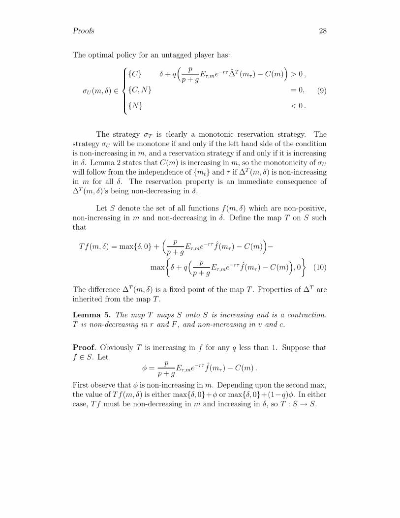
Proofs 28

The optimal policy for an untagged player has:

σU (m, δ) ∈

C δ + q( p

p + gEτ,me−rτ∆T (mτ ) − C(m)

)

> 0 ,

C, N = 0,

N < 0 .

(9)

The strategy σT is clearly a monotonic reservation strategy. Thestrategy σU will be monotone if and only if the left hand side of the conditionis non-increasing in m, and a reservation strategy if and only if it is increasingin δ. Lemma 2 states that C(m) is increasing in m, so the monotonicity of σU

will follow from the independence of mt and τ if ∆T (m, δ) is non-increasingin m for all δ. The reservation property is an immediate consequence of∆T (m, δ)’s being non-decreasing in δ.

Let S denote the set of all functions f(m, δ) which are non-positive,non-increasing in m and non-decreasing in δ. Define the map T on S suchthat

Tf(m, δ) = maxδ, 0 +( p

p + gEτ,me−rτ f(mτ ) − C(m)

)

−

max

δ + q( p

p + gEτ,me−rτ f(mτ ) − C(m)

)

, 0

(10)

The difference ∆T (m, δ) is a fixed point of the map T . Properties of ∆T areinherited from the map T .

Lemma 5. The map T maps S onto S is increasing and is a contraction.T is non-decreasing in r and F , and non-increasing in v and c.

Proof. Obviously T is increasing in f for any q less than 1. Suppose thatf ∈ S. Let

φ =p

p + gEτ,me−rτ f(mτ ) − C(m) .

First observe that φ is non-increasing in m. Depending upon the second max,the value of Tf(m, δ) is either maxδ, 0+φ or maxδ, 0+(1−q)φ. In eithercase, Tf must be non-decreasing in m and increasing in δ, so T : S → S.

Proofs 29

To see that T is a contraction map, consider f and g in S and pick astate m and reward u. Let z = p/(p+ g). First, suppose that for both f andg, the maxima are the left hand terms. Then

Tf(m, δ) − Tg(m, δ) =p(1 − q)

p + gEτ,me−rτ

(

f(mτ ) − g(mτ ))

Thus ||f − g|| < ε implies |Tf(m, δ) − Tg(m, δ)| ≤ z(1 − q)ε. Next, supposethat both maxes are the right hand terms, C(m). Then ||f − g|| < ε implies|Tf(m, δ) − Tg(m, δ)| ≤ zε. Next, suppose that the max for f is the lefthand term and the max for g is the right hand term. That is,

δ − qC(m) +pq

p + gEτ,me−rτ f(mτ ) ≥ 0

≥ δ − qC(m) +pq

p + gEτ,me−rτ g(mτ )

Calculating with this inequality shows that if ||f − g|| < ε, then

(1 − q)zε ≤ ||Tf − Tg|| ≤ zε

The same result obtains if the max for f is on the right and for g on the left.Thus the operator T on S contracts at rate z < 1.

The remaining effects of parameter changes are straightforward cal-culations. The effect of increasing F follows from the fact that if h(x) is non-decreasing in x, then the expectation Eh is non-decreasing as the probabilitydistribution increases in the sense of first-order stochastic dominance.

All the existence and comparative statics results will be derived fromthe Tarski’s fixed point theorem for increasing functions on complete lattices.The required monotonicity is a consequence of the following lemma:

Lemma 6. For all f in S, Tf is non-decreasing in the death rates of themtt≥0 process.

The proof is another kind of coupling argument.

Proofs 30

Proof. It suffices to show that φ is non-decreasing in the death rates of m.Since the random time τ is independent of the mt process, it suffices to showthat for any time T and and non-increasing function f(m), the expectationEmf(mT ) is non-decreasing in the death rates µm.

Let λxm, mux

mN−1m=0 and λy

m, muym

N−1m=0 be two sets of birth and death

rates such that λxm ≥ λy

m and µxm ≤ µy

m. Thus the first set has higherbirth and lower death rates than the second. Let λm = maxλx

m, λym and

µm = maxµxm, µy

m. (The Lemma only requires λxm = λy

m, but I may findthis fact useful later.)

Construct the coupling xt, ytt≥0 as follows. The processes begin inthe same state, that is, x0 = y0. Whenever xt = yt = m, births arrive at rateλm and deaths arrive at rate µm. When a birth arrives, process x incrementswith probability λx

m/λm and y increments with probability λym/λm. Whenever

xt 6= yt, the two processes evolve independently according to their respectivebirth and death rates. It is easy to see that each marginal process xtt≥0

and ytt≥0 evolves according to its own birth and death rates, and thatalmost surely, xt ≥ yt. Consequently, almost surely f(xt) ≤ f(yt), and sothis is true in expectation as well.

This is enough to prove theorems 1 and 2. The existence of equilibriumwill follow from Zhou’s (1994) extension of Tarski’s fixed point theorem. Wewill follow Topkis (1998). It is also convenient to use lattice arguments toget the effects of parameter changes on ∆T even though the existence of afixed point for T is guaranteed by the Contraction Mapping Theorem.

First, the set S is a complete lattice under the pointwise “at least asbig as” order. It follows from the fixed point theorem and Lemma 5 thatT has fixed points, the set of fixed points can be totally ordered, and thatthe least and greatest fixed points are non-decreasing in r and F , and non-decreasing in v and c. It follows from Lemma 6 that the greatest and leastfixed points are non-decreasing in the death rates of the mt process. SinceT is a contraction, it has in fact only one fixed point, ∆T , and ∆T varies asjust described with the parameters.

Since ∆T (m, δ) is non-increasing in m and since the time τ is inde-pendent of the mt process, it follows from lemma monotone that φ is non-increasing in m0. If c(m) is not constant it is strictly increasing in m. From

Proofs 31

equation 9 it follows that the optimal policies for an untagged player are allmonotonic reservation strategies.

Although we cannot totally order all strategies, the previous argu-ment shows that all best responses are monotonic strategies, that σU miyesin at most one state, and that σT ≡ 1. The set of all such strategies istotally ordered by , the “more criminal than” ordering. Each such σ canbe characterized by a pair (m, p) for σU with p > 0 such that σU (m′) is 0 form′ > m, 1 for m′ < m and p for m′ = m. Then σ σ′ if and only if m′ > mor m′ = m and p′ ≥ p.

Now that the strategy set has been reduced to degrees of criminality,we can see how “being more criminal” provides a strategic complementarity.We will demonstrate that individual i’s best response correspondence B(σU )is increasing in the order . Define

B(σU) =

1 if δ + q( p

p + gEτ,me−rτ∆T (mτ ) − C(m)

)

> 0 ,

[0, 1] if = 0,

0 if < 0 .

This correspondence is increasing in σ. If σ′ σ, then as equations (1) and(2) show, the birth rates for the state process remain the same and the deathrates increase. It follows from Lemma 6 that φ increases, and thereforeso does the threshold state. Similarly B(σ) is increasing in r and F , anddecreasing in v, and c.

Zhou’s fixed point theorem requires that B(σU ) is increasing in itsargument, which we have shown, and that B(σU) has the lattice propertyof being sub-complete. This is guaranteed by the fact that the strategyset is compact in the natural product topology and totally ordered, andthat the ordering is continuous in the natural topology.19 Consequently thebest-response correspondence has a fixed point, and any such fixed pointis an equilibrium. This proves Theorem 1. The comparative statics result,Theorem 2, follows immediately from Topkis (1998, Theorem 2.5.2) and thecomparative statics of φ.

Proof of Theorem 3 and the Corollary: The birth rates for the populationprocess are fixed by the parameters of the model. Only the death rates

Proofs 32

depend on the strategy, and they are non-decreasing in the criminality ofthe strategy. We are given odds ratios rn for each adjacent pair of N + 1states ordered from 0 to N : π(n) = π(n−)rn, and we want to infer that ifone ri increases, then for any number A the probability Prn ≥ A does notdecrease. To see this, write

Prn ≥ A =

∑N

l=A r1 · · · rl

1 +∑N

k=1 r1 · · · rk

Differentiating with respect to ri shows that Prn ≥ A increases in ri. Mak-ing a strategy more criminal does not lower and can raise a death rate, which(weakly) decreases some odds ratios. The Theorem follows from Theorem 2.

To prove the corollary, observe that the long run crime rate η(n)decreases in n. The expectation of a decreasing function increases as thedistribution falls with respect to first order stochastic dominance.

6.2 Theorem 4

The expected present value of the cost of being caught is bounded above byqv+qc(0)/r. Any crime opportunity with a reward u exceeding this value willbe accepted. The hypothesis of the theorem is that the occurrence of suchopportunities is a positive probability event. Thus in each state, the deathrate is at least pq

(

1 − F (qv + qc(1)/r))

> 0. On the other hand, as g → 0the birth rates are converging to 0 in each state. In the limit process, 0 isthe only recurrent state, and the unique ergodic distribution puts all its massat 0. In this limit, every individual is tagged, and so equilibrium behavior isgiven by σ∗. For g sufficiently small, the fraction of criminal opportunitiescoming to untagged individuals is very small. Since the birth rates are verysmall, the invariant distribution, given by (3), is nearly point mass at 0. Thelong run crime rate is continuous in the parameter values and with respectto the invariant distribution. At g = 0, it is η∗.

As g becomes large, C(m) converges to 0, and so it is apparent fromequations (6) and (7) that VC(m, δ)−VN(m, δ) converges to δ for all m. Thusfor each state the threshold utility converges to qv. Since qv is a continuitypoint of F , the death rate in each state converges to pq

(

1−F (qv))

, the death

Proofs 33

rate which would result from decision rule σ∗. The birth rate in each stateis converging to 0, and so in the limit, the invariant distribution has pointmass at 1, the equilibrium strategy has σC = σ∗, and the long run crime rateis η∗.

6.3 Computing Equilibria

Best responses to a given strategy ρ = (ρU , ρT ) used by the population aredetermined by the sign of the expression

δ + q( p

p + gEτ,me−rτ∆T (mτ ) − C(m)

)

The dependence of this expression on ρ is through the evolution of the stateprocess mt, which appears both in the term Eτ,me−rτ∆T (mτ ) and in theterm C(m). The operator T defined in equation (10), whose fixed point is∆T is a contraction map, so in principle one should be able to compute thefunction for various values of ρ. The trick to the computation is to get anexpression for the operator. This requires computing, for a given functionf(m, δ), the expression Eτ,mf(mτ ), and computing for the cost function cthe expression Eτ,m

∫ τ

0e−rtc(mt) dt. Fortunately the apparatus of birth-death

processes provides a convenient computational technique for producing theseexpressions. To illustrate the technique, consider C(m).

Begin in state m at time 0, and define a time σ which is exponentiallydistributed with parameter λ(m) + µ(m) + p + g, where λ(m) and µ(m) arethe birth and death rates, respectively, for the mt process with strategy ρ,as given by equations (1) and (2). Then

C(m) = Eτ,m

∫ τ

0

e−rtc(mt) dt

= Eσ

∫ σ

0

e−rtc(m) dt + Eσ

e−rσ( λ(m)

λ(m) + µ(m) + p + gC(m+) +

µ(m)

λ(m) + µ(m) + p + gC(m−)

)

=1

λ(m) + µ(m) + p + gc(m) +

34

λ(m)

λ(m) + µ(m) + p + g + rC(m+) +

µ(m)

λ(m) + µ(m) + p + g + rC(m−)

This recursion formula says, compound the flow cost from now until time σ.At time σ either a criminal opportunity or untagging has arrived, σ = τ , orthe mt process has moved: up with proability λ(m)/λ(m) + µ(m) + p + gand down with probability µ(m)/λ(m)+µ(m)+ p+ g. In the first case, stopcompounding. In the second and third cases, just add on C(m+) or C(m−),appropriately discounted.

This formula for C(m) suggests examining the operator O(f) definedsuch that:

O(f)(m) =1

λ(m) + µ(m) + p + gc(m) +

λ(m)

λ(m) + µ(m) + p + g + rf(m+) +

µ(m)

λ(m) + µ(m) + p + g + rf(m−)

This operator is a contraction on the space of functions from Ω to R, and itsfixed point is C(m). This operator can easily be iterated on the computer toapproximate C(m). A similar operator can be iterated to find Eτ,mf(m) fora given function f . With these functions in hand, T (f) can be computed.And iterating T gives ∆T , from which best responses and equilibria are easilycomputed.

Notes

1Cowell (1990), McGraw and Scholz (1992) and Schwartz and Orleans(1966) are a few of the many studies demonstrating this effect.

2Given decision rules for all individuals, the process nt∞t=0 describing the

number of untagged individuals in the entire population can be constructedsimilarly.

35

3It makes no qualitative difference whether we assume this or µ = µT .

4Other parameter values are: p = 0.7, g = 0.002 c(m) = 2.5m, r = 0.15,ε = 0.01, uh = 5.0 and ul = 1.0. In this plot, N = 200.

5Other parameter values are: p = 0.65, q = 0.95 c(m) = 2.0m4, r = 0.01,ε = 0.01, uh = 5.0 and ul = 1.0. In this plot, N = 200.

6See Book (1999) and Brilliant (1989).

7See Blume and Durlauf (1998).

8This is closely related to statistical discrimination models.

9For instance, if sufficiently few individuals are marked most of the time,the incidence of the mark may fall below the threshold of social attentionwhich would invoke a stigmatic response.

10Lessig (1995, p. 965).

11See Book (1999) and Brilliant (1989) for startling examples of this recentphenomenon.

1221 U.S.C. §862(a). Those wishing to remove the ban must be able to“prove” rehabilitation, a difficult and potentially costly undertaking. Indi-vidual states may opt out of this provision. As of January 2002, 19 stateshave left the ban in place, and some of those states which have modified theban have in fact extended its coverage. See Hirsch (2002, Chapter 1).

1315 U.S.C. 1681c(a)(5). See Hirsch (2002, Chapter 2).

14See Goffman (1963, p. 12.).

15Newman (1999, p. 104). “Burger Barn” is a pseudonym for a nationalchain of fast food restaurants.

16For instance, the Anti-Drug Abuse Act of 1988 punished simple pos-session of five grams of crack with a mandatory-minimum sentence of sixtymonths in prison. Possession of any quantity of any other substance bya first-time offender is a misdemeanor punished by a maximum of twelvemonths in prison. See 21 U.S.C. §844(a) (1994). One estimate has it that

36

nearly one-third of young male African-Americans between the ages of 20and 29 are in prison, jail, or on probation or parole. See Mauer and Huling(1995).

17 Beginning in 1993 the New York City Police Department began ag-gressive enforcement of “public order” violations such as public drunkenness,prostitution, aggressive panhandling and the like. City officials and somecriminologists believe this strategy is responsible for New York’s above aver-age rate reductions burglaries, robberies and murder. See Kahan (1997).

18The exceptional set is Matsui and Matsuyama (1995), Hofbauer andSorger (2000), and for stochastic population games, Blume (1995).

19It has to be “subcomplete”. See Topkis (1998), Theorem 2.5.1. Thestrategy space itself must also be a complete lattice, which is guaranteedagain by order-continuity, its compactness, and that the order is complete.

References

Anderson, E. (1990): Streetwise: Race, Class, and Change in an UrbanCommunity. University of Chicago Press, Chicago.

Becker, G. S. (1968): “Crime and Punishment: An Economic Approach,”Journal of Political Economy, 76, 169–217.

Blume, L. E. (1993): “The Statistical Mechanics of Strategic Interaction,”Games and Economic Behavior, 4, 387–424.

Blume, L. E. (1995): “Evolutionary Equilibrium with Forward-LookingPlayers,” Cornell University.

Blume, L. E., and S. Durlauf (1998): “Equilibrium Concepts for SocialInteraction Models,” forthcoming, International Game Theory Review.

Book, A. S. (1999): “Shame on You: An Analysis of Modern Shame Pun-ishment as an Alternative to Incarceration,” William and Mary Law Re-view, 40, 653–686.

37

Brilliant, J. A. (1989): “The Modern Day Scarlet Letter: A CriticalAnalysis of Modern Probation Conditions,” Duke Law Journal, pp. 1357–1384.

Cowell, F. A. (1990): Cheating the Government: The Economics of Eva-sion. MIT Press, Cambridge MA.

Ethier, S. N., and T. G. Kurtz (1986): Markov Processes: Characteri-zation and Convergence. Wiley-Interscience, New York.

Goffman, E. (1963): Stigma: Notes on the Management of Spoiled Identity.Simon and Schuster, New York.

Hirsch, Amy E., et. al. (2002): “Closing the Door: Barriers Facing Par-ents with Criminal Records,” Center for Law and Social Policy, availableat http://www.clasp.org.

Hofbauer, J., and G. Sorger (2000): “A Differential Game Approach toEquilibrium Selection,” International Game Theory Review, forthcoming.

Kahan, D. M. (1997): “Social Influence, Social Meaning, and Deterrence,”Virginia Law Review, 83, 349–95.

Kandori, M., G. Mailath, and R. Rob (1993): “Learning, Mutationand Long Run Equilibrium in Games,” Econometrica, 61, 29–56.

Kingman, J. F. C. (1993): Poisson Processes. Oxford University Press,New York.

Lessig, L. (1995): “The Regulation of Social Meaning,” University ofChicago Law Review, 62, 943–1045.

Link, B. G., and J. C. Phelan (2001): “Conceptualizing Stigma,” AnnualReview of Sociology, 27, 363–85.

Matsui, A., and K. Matsuyama (1995): “An Approach to EquilibriumSelection,” Journal of Economic Theory, 65, 415–434.

Mauer, M., and T. Huling (1995): Young Black Americans and the Crim-inal Justice System: Five Years Later. The Sentencing Project, New York,NY, Report #9070.

38

McGraw, K. M., and J. T. Scholz (1992): “Taxpayer Adaptation tothe 1986 Tax Reform Act: Do New Tax Laws Affect the Way TaxpayersThink About Taxes?,” in Why People Pay Taxes: Tax Compliance andEnforcement, ed. by J. Slemrod. University of Michigan Press, Ann Arbor.

Newman, K. S. (1999): No Shame in My Game: The Working Poor in theInner City. Random House, New York.

Sampson, R. J., and W. B. Groves (1989): “Community Structure andCrime: Testing Social Disorganization Theory,” American Journal of So-ciology, 94(4), 774–802.

Schwartz, R. D., and S. Orleans (1966): “On Legal Sanctions,” Uni-versity of Chicago Law Review, 34, 296–99.

Topkis, D. M. (1998): Supermodularity and Complementarity. PrincetonUniversity Press, Princeton, NJ.

Young, H. P. (1993): “The Evolution of Conventions,” Econometrica, 61,57–84.

Zhou, L. (1994): “The set of Nash equilibria of a supermodular game is acomplete lattice,” Games and Economic Behavior, 7, 295–300.

Author: Lawrence Blume Title: Stigma and Social Control Reihe Ökonomie / Economics Series 119 Editor: Robert M. Kunst (Econometrics)

Associate Editors: Walter Fisher (Macroeconomics), Klaus Ritzberger (Microeconomics) ISSN: 1605-7996 © 2002 by the Department of Economics and Finance, Institute for Advanced Studies (IHS), Stumpergasse 56, A-1060 Vienna • ( +43 1 59991-0 • Fax +43 1 5970635 • http://www.ihs.ac.at

ISSN: 1605-7996