Von Neumann – Morgenstern Expected Utility

I. Introduction, Definitions, and Applications

Decision TheorySpring 2014

Origins

Blaise Pascal, 1623 – 1662

I Early inventor of the mechanicalcalculator

I Invented Pascal’s Triangle

I Invented expected utility, hedgingstrategies, and a cynic’s argumentfor faith in God all at once.

Pascal’s Wager

God exists God does not existlive as if he does −C +∞ −C

live for yourself U −∞ U

Origins

Daniel Bernoulli

I Mechanics

I Hydrodynamics — Kinetic Theoryof Gases

I Bernoulli’s Principle

The St. Petersburg Paradox

A coin is tossed until a tails comes up. How much would you payfor a lottery ticket that paid off 2n dollars if the first tails appearson the n’th flip?

The St. Petersburg Paradox

Average payoff from paying c :

E =1

2· (w − c) +

1

4· (w + 2− c) +

1

8· (w + 4− c) + · · ·

=1

2+

1

2+

1

2+ · · ·+ w − c

=∞

Bernoulli’s solution:

E =1

2· log+(w − c) +

1

4· log+(w + 2− c) +

1

8· log+(w + 4− c) + · · ·

This is finite for all w and c. (log+(x) = log max{x , 1}.)

The St. Petersburg Paradox

This doesn’t solve the problem. Average payoff from paying c :

E =1

2· log+(w + exp 20 − c) +

1

4· log+(w + exp 21 − c)

+1

8· log+(w + exp 22 − c) + · · ·

=∞

Solution:

I Utility bounded from above.

I Restrict the set of gambles.

Preferences on Lotteries

X = {x1, . . . , xN} — A finite set of prizes.

P = {p1, . . . , pN} — A probability distribution.

P = {p1, . . . , pN} — pi is the probability of xi .

(0, 0, 1) : x3

(0, 1, 0) : x2 (1, 0, 0) : x1

Preferences on Lotteries

x3

x2 x1

For fixed prizes, indifference curves are linear in probabilities.

Lotteries on R

A simple lottery is p = (p1 : x1, . . . , pK : xK ) where x1, . . . , xK areprizes in R and p1, . . . , pK are probabilities. Let L denote the setof simple lotteries. Let

u : X → R

and V (p) =∑k

u(xk)p(xk).

This is the expectation of the random variable u(x) when the therandom variable x is described by the probability distribution p.

Lotteries on R

How do we see that this is “linear” in lotteries? For 0 < α < 1 andlotteries p = (p1 : x1, . . . , pK : xK ) and q = (q1 : y1, . . . , qL : yL),define

zm =

{xm for m ≤ K ,

ym−K for K < m ≤ K + L.

and

αp ⊕ (1− α)q = (r1 : z1, . . . , rK+L : zK+L)

where

rm =

{αpm for m ≤ K ,

(1− α)qm−K for K < m ≤ K + L.

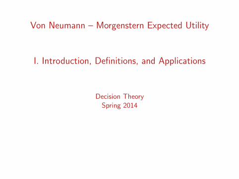
Lotteries on R

V (αp ⊕ (1− α)q) =M∑

m=1

rmu(zm)

=K∑

m=1

αpmu(xm) +K+L∑

m=K+1

(1− α)qm−Ku(ym−K )

= α

K∑k=1

pku(xk) + (1− α)L∑

l=1

qlu(yl)

= αV (p) + (1− α)V (q).

Attitudes Towards Risk

V (p) = Ep{u} =∑

x∈supp p

u(x)p(x) P = {p ∈ L : V (p) <∞}.

Definition: An individual is risk averse iff for all p ∈ P,Ep{u} ≤ U(Ep{x}). He is risk-loving iff Ep{u} ≥ u(Ep{x}).

Theorem A: A Decision-Maker is risk averse iff u is concave, andrisk-loving iff u is convex.

Definition: The certainty equivalent of a lottery p is the sure-thingamount which is indifferent to p: CE{p} = u−1(V (p)).

Theorem B: A DM is risk-averse iff for all p ∈ P, CE{p} ≤ Ep{u}.

Proofs are here.

Certainty Equivalents

x2x1 ExCE

Eu(x)

u(Ex)

Measuring Risk Aversion

Definition: The Arrow-Pratt coefficient of absolute risk aversion atx is rA(x) = −u′′(x)/u′(x). The coefficient of relative risk aversionis rR(x) = xrA(x).

CARA utility: u(x) = − exp{−αx}.

CRRA utility: u(x) =

1γ x

γ , γ ≤ 1, γ 6= 0

log x .

When utility is CARA and P is the set of normal distributions,

CE (F ) = µ− 1

2ασ2.

Comparing Attitudes to Risk

Theorem C: The following are equivalent for two utility functionsu1 and u2 when p ∈ P:

1. u1 = g ◦ u2 for some concave g ;

2. CE1(p) ≤ CE2(p) for all p ∈ P;

3. rA,1(x) ≥ rA,2(x) for all x ∈ R.

How should risk aversion vary with wealth?

rA(x |w) = −u′′(x + w)/u′(x + w).

How would you expect this to behave as a function of w?

Click for the Proof of Theorem C.

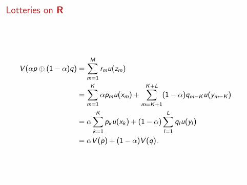
Applications

A risk-averse DM has wealth w > 1 and may lose 1 withprobability p. He can buy any amount of insurance he wants sat qper unit. His expected utility from buying d dollars of insurance is

EU(d) = (1− p)u(w − qd) + pu(w − qd − (1− d)

).

Under what conditions will he insure, and for how much of the loss?

Definition: Insurance is actuarially fair, sub-fair, or super-fair if theexpected net payout per unit, p − q, is = 0, < 0, or > 0,respectively.

Definition: Full insurance is d = 1.

Sub-Fair Insurance

Use derivatives to locate the optimal amount of insurance.

EU ′(d) = −(1− p)u′(w − qd)q + pu′(w − qd − (1− d)

)(1− q).

Suppose q > p.

EU ′(1) = u′(w − q)(−(1− p)q + p(1− q)

)= u′(w − q)(p − q) < 0

EU ′(0) = −(1− p)u′(w)q + pu′(w − 1)(1− q)

= pu′(w − 1)−((1− p)u′(w) + pu′(w − 1)

)q > · · · p

= p(1− p)(u′(w − 1)− u′(w)

)> 0.

Why is u′(w − 1)− u′(w) > 0?

Fair Insurance

Suppose q = p.

EU ′(1) = u′(w − q)(p − q) = u′(w − q)(p − p)0.

Full insurance is optimal.

Optimal Portfolio Choice

A risk-averse DM has initial wealth w . There is a risky asset thatpays off z for each dollar invested. z is drawn from a distributionwith a probability function p. If he invests in α units of the asset,he gets

U(α) = Epu(w + α(z − 1)

)Which is concave in α. The optimal investment α∗ solves

U ′(α∗) = Epu′(w + α(z − 1)

)(z − 1) = 0.

Optimal Portfolio Choice

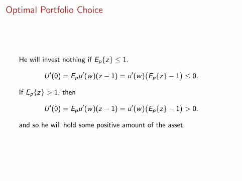
He will invest nothing if Ep{z} ≤ 1.

U ′(0) = Epu′(w)(z − 1) = u′(w)

(Ep{z} − 1

)≤ 0.

If Ep{z} > 1, then

U ′(0) = Epu′(w)(z − 1) = u′(w)

(Ep{z} − 1

)> 0.

and so he will hold some positive amount of the asset.

Optimal Portfolio Choice

Theorem: More risk individuals hold less of the risky asset, otherthings being equal.

Proof: Suppose DM 1 has concave utility u1, and individual 2 ismore risk-averse. Then u2 = g ◦ u1. There is no loss of generalityin assuming g ′(u1) = 1 at u1 = u1(w). For every α,

U ′2(α)− U ′1(α) = Ep

(g ′(u1)− 1

)u′1(w + α(z − 1)

)(z − 1)

Now z < 1 iff w + α(z − 1) < w iff u1(w + α(z − 1) < u1(w) iffg ′(u1(w + α(z − 1)

)> g ′

(u1(w), so the expression inside the

integral is always negative, and so U ′2(α) < U ′1(α) for all α. Inparticular, when α is optimal for DM 1, U ′2(α) < 0, so the optimalα for DM 2 is less.

Comparative Statics

Utility over portfolios depends upon the DM’s initial wealth.

U(α;w) = Epu(w + α(z − 1)

)The DM’s preferences have decreasing absolute risk aversion ifwhenever w ′ > w , U( · ;w ′) is less risk-averse then U( · ;w).

Theorem: If the DM has decreasing absolute risk aversion, then α∗

increasing in w .

Risk Aversion

PROOFS

Concavity and Risk Aversion

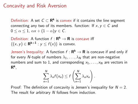
Definition: A set C ⊂ Rk is convex if it contains the line segmentconnecting any two of its members. function: If x , y ∈ C and0 ≤ α ≤ 1, αx + (1− α)y ∈ C .

Definition: A function f : Rk → R is concave iff{(x , y) ∈ Rk+1 : y ≤ f (x)} is convex.

Jensen’s Inequality: A function f : Rk → R is concave if and only iffor every N-tuple of numbers λ1, . . . , λN that are non-negativenumbers and sum to 1, and corresponding x1, . . . , xN are vectors inRk,

N∑n=1

λnf (xn) ≤ f

(N∑

n=1

λnxn

).

Proof: The definition of concavity is Jensen’s inequality for N = 2.The result for arbitrary N follows from induction.

Concavity and Risk Aversion

Proof of Theorem A: For concave functions this is Jensen’sinequality. A function f is convex iff −f is concave. Suppose u isconvex. From Jensen’s inequality, u is convex iff

∑n

λn(−u(xn)

)≤ −u

(∑n

λnxn

)

iff

∑n

λn(u(xn)

)≥ u

(∑n

λnxn

),

iff the DM is risk-loving.

Concavity and Risk Aversion

Proof of Theorem B: From Theorem A, if the DM is risk-averse,then Epu(x) ≤ u(Epx). By definition, u(CEp) = Epu(x) ≤ u(Epx),and since u is increasing, CE (p) ≤ Epx .

Back

Comparing Attitudes to Risk

1 iff 2: u2 = g ◦ u1 if and only if for all p,Epu2 = Epg ◦ u1 ≤ g (Eu1). Then

u2(CE2(p)

)= Epu2 = Epg ◦ u1

≤ g(Epu1

)= g ◦ u1

(CE1(p)

)= u2

(CE1(p)

).

Since u2 is increasing, CE2(p) ≤ CE1(p).

1 iff 3: Since u1 and u2 are increasing functions, there is anincreasing function g such that u2 = g ◦ u1. The chain rule impliesthat r2 = r1 − g ′′/g ′, so g ′′ = (r1 − r2)g ′. Since g ′ > 0, g ′′ ≤ 0 iffr2 ≥ r1.

Back