Stephen J. De Canio-Economic Models of Climate Change_ A Critique (2003).pdf

Economic Models ofClimate Change

A Critique

Stephen J. DeCanio

Economic Models of Climate Change

1403_963363_01_pre.qxd 6/30/03 11:02 AM Page i

This page intentionally left blank

Economic Models ofClimate ChangeA Critique

Stephen J. DeCanioProfessor of EconomicsUniversity of CaliforniaSanta BarbaraUSA

1403_963363_01_pre.qxd 6/30/03 11:02 AM Page iii

© Stephen J. DeCanio 2003

All rights reserved. No reproduction, copy or transmission of thispublication may be made without written permission.

No paragraph of this publication may be reproduced, copied ortransmitted save with written permission or in accordance with theprovisions of the Copyright, Designs and Patents Act 1988, or under theterms of any licence permitting limited copying issued by the CopyrightLicensing Agency, 90 Tottenham Court Road, London W1T 4LP.

Any person who does any unauthorised act in relation to this publicationmay be liable to criminal prosecution and civil claims for damages.

The author has asserted his right to be identified as the author of thiswork in accordance with the Copyright, Designs and Patents Act 1988.

First published 2003 byPALGRAVE MACMILLAN175 Fifth Avenue, New York, N.Y. 10010 and Houndmills, Basingstoke,Hampshire RG21 6XSCompanies and representatives throughout the world

PALGRAVE MACMILLAN is the global academic imprint of the PalgraveMacmillan division of St. Martin’s Press, LLC and of Palgrave MacmillanLtd. Macmillan® is a registered trademark in the United States, UnitedKingdom and other countries. Palgrave is a registered trademark in theEuropean Union and other countries.

ISBN 1–4039–6335–5 hardbackISBN 1–4039–6336–3 paperback

This book is printed on paper suitable for recycling and made from fullymanaged and sustained forest sources.

A catalogue record for this book is available from the British Library.

Library of Congress Cataloging-in-Publication Data

DeCanio, Stephen J.Economic models of climate change : a critique / Stephen J. DeCanio.

p. cm.Includes bibliographical references and index.ISBN 1–4039–6335–5 – ISBN 1–4039–6336–3 (pbk.)1. Environmental policy – Economic aspects. 2. Climatic changes –

Economic aspects. I. Title.

GE170.D44 2003363.738¢74¢011 – dc21

2003040533

10 9 8 7 6 5 4 3 2 112 11 10 09 08 07 06 05 04 03

Printed and bound in Great Britain byAntony Rowe Ltd, Chippenham and Eastbourne

1403_963363_01_pre.qxd 6/30/03 11:02 AM Page iv

For the future generations

1403_963363_01_pre.qxd 6/30/03 11:02 AM Page v


Contents

List of Tables ix

List of Figures x

Acknowledgments xi

1 An Overview of the Issues 11.1 General equilibrium analysis 41.2 Equity and efficiency 81.3 Outline of the book 13

2 The Representation of Consumers’ Preferences and Market Demand 162.1 Introduction 162.2 Elements of the “outside” critique 172.3 The “inside” critique 282.4 Conclusions and implications for policy 56

3 The Treatment of Time 583.1 The problem 583.2 Three ways to represent time 623.3 The Arrow–Debreu approach: all transactions occur

at the “beginning” 633.4 Overlapping generations: transactions occur in the

present, accounting for past history and expectations 743.5 Models with a social planner or infinitely lived agents 843.6 Conclusions and implications for policy 89

4 The Representation of Production 944.1 Introduction 944.2 The modern theory of the firm 974.3 Aggregation problems 1034.4 A more realistic characterization of production 1064.5 Conclusions and implications for policy 123

vii

1403_963363_01_pre.qxd 6/30/03 11:02 AM Page vii

5 The Forecasting Performance of Energy-Economic Models 1265.1 Introduction 1265.2 The long-term predictive power of economic models

is limited 1275.3 Predictions of the costs of greenhouse gas reductions

and other regulatory policies 1455.4 Conclusions and implications for policy 151

6 Principles for the Future 153

Notes 161

References 178

Index 195

viii Contents

1403_963363_01_pre.qxd 6/30/03 11:02 AM Page viii

List of Tables

2.1 Equilibrium prices, incomes, and Gini index of inequality,symmetrical 5 ¥ 5 economy 37

2.2 Equilibrium prices, incomes, and utility rankings, 5 ¥ 5economy, asymmetrical endowments 43

2.3 Equilibrium prices, incomes, and utility rankings, 5 ¥ 5economy, asymmetrical endowments, and unequal substitution elasticities 45

2.4 Representation of preferences in integrated assessment models 54

3.1 Time structure of consumption in OLG model 754.1 Number of digraphs with n vertices 1124.2 Tests of null hypothesis that all 100 populations are from

the same fitness distribution 1194.3 Results of head-to-head competition, 3 species, 100 runs

of 500 generations each, A = 500, c = 3.5, r = 0.1 1225.1 Actual energy usage compared to 1974–76 forecasts 1335.2 Actual and forecast crude oil prices, 1995 dollars/bbl 1355.3 Actual and forecast total energy consumption, United

States, quadrillion BTUs 1365.4 Energy consumption projections for the United States,

NERA compilation (publication dates 1974–77) 1375.5 Projections of primary and delivered fuel prices and

errors: five major energy studies of 1982–83 (all prices except world oil in 1996 dollars per million BTU) 139

5.6 Average absolute percentage errors from 2000 AEO forecastevaluation: AEO 1982 to AEO 2000 140

5.7 Estimated regression equation, pat = a0 + a1pf

t,t-1 + et, 1985–99,world oil price and natural gas wellhead price from AnnualEnergy Outlook 142

5.8 Case study results on the accuracy of regulatory forecasts 1465.9 Range of estimates of 2010 GDP effects of GHG reduction

policies, EMF-12 and EMF-16 148

ix

1403_963363_01_pre.qxd 6/30/03 11:02 AM Page ix

List of Figures

2.1(a) Utility surface for two goods with high elasticity of substitution 31

2.1(b) Utility surface for two goods with low elasticity of substitution 32

2.2 Excess demand for good 1 as a function of p1 and a11 362.3 Demand surface for agent 1 and good 1, p3, p4, and p5

at equilibrium 7 402.4 Moving to equilibrium 483.1 Alternative paths to the steady state: Cobb–Douglas

case 823.2 Chaotic equilibria: CES utility case 834.1 Diffusion of innovation through an organization 1114.2 Chromosomes of two parents and offspring, size 6

organization 1134.3 Typical histograms of fitness scores from evolved

populations 1174.4 15 vs. 16 vs. 17 proportionate selection with no elites

and type 1 scaling 1205.1 Comparison of actual and forecast oil prices, 1992–99 1455.2 Variations in GDP impact: 162 simulations across 16

models 1495.3 US cost and savings components of a least-cost Kyoto

strategy with global trading, 2010 151

x

1403_963363_01_pre.qxd 6/30/03 11:02 AM Page x

Acknowledgments

Many colleagues and friends have contributed directly or indirectly tothis book. As the notes and references throughout the text make clear,I owe a primary debt to those researchers who have communicated theirinsights through the scholarly literature. That literature has become so voluminous that I am sure I have missed many pertinent items; Iapologize in advance for any such omissions.

A number of economists have contributed in a more personal way to my understanding of climate economics and modeling issues ingeneral, particularly Gale Boyd, Richard Howarth, Florentin Krause, PaulKrugman, Richard Norgaard, Irene Peters, Alan Sanstad, and JeffreyWilliams. Members of the Economics Department at UCSB who haveoffered helpful advice are Henning Bohn, H.E. Frech III, Rajnish Mehra,and Jati Sengupta. Scholars outside the field of economics have providedmuch valuable input. Penelope Canan, Jeffrey Friedman, JonathanKoomey, Kai Lee, Amory Lovins, Claudia Pahl-Wostl, Nancy Reichman,and Stephen Schneider have all widened my outlook. Friends outside ofacademia have also left their mark, including John Gliedman and KeithWitt. I relied on the advice of Diana Strazdes in selecting the cover art.I will never forget the inspiration and training I received from my pro-fessors at MIT over 30 years ago, especially Peter Temin and Franklin M.Fisher. I learned more than I was ever able to acknowledge from mydeceased former colleagues M. Bruce Johnson and William N. Parker.

I want to offer special thanks to several of my former and currentgraduate students whose contributions have been invaluable. KeyvanAmir-Atefi provided criticisms and perspective throughout the project,and did an outstanding job of programming the evolutionary modelsdescribed in Chapter 4. Yusuf Okan Kavuncu assisted in the pro-gramming for Chapter 3 and in the process significantly improved myunderstanding of overlapping-generations models. Andrea Lehmanworked on some of the statistical analysis of Chapter 5, helping as much with material that was cut as with what remained. CatherineDibble, William E. Watkins, Glenn Mitchell, and Ben Alamar showedme various aspects of the potential scope and power of computationalmethods in economics.

The book has a strong policy orientation. I first became involved in the economics of global environmental protection when I had the

xi

1403_963363_01_pre.qxd 6/30/03 11:02 AM Page xi

honor to serve as a Senior Staff Economist at the Council of EconomicAdvisers during 1986–87. Several people who were at the US Environ-mental Protection Agency during that time influenced the course of mycareer, including Steve Andersen, Eileen Claussen, and John Hoffman.In recent years, I have benefited greatly from the insight and patienceof John A. “Skip” Laitner, Senior Economist for Technology Policy inthe EPA Office of Atmospheric Programs, who was the Project Directorof EPA Grant X-82830501-0 that provided support for a major portionof the project.

Some of the results from Chapter 2 have been presented at seminarsand conferences held at the US Environmental Protection Agency, theUCSB Department of Geography, the Energy and Resources Group atthe University of California at Berkeley, and the UCLA ComputationalSocial Sciences Conference in Lake Arrowhead. Feedback from partici-pants in those gatherings was greatly appreciated.

Acknowledgment is given to the World Resources Institute for per-mission to reproduce Figure 5.2, the International Project for Sustain-able Energy Paths for Figure 5.3, and The Johns Hopkins University Pressfor most of Table 5.1 (Ascher, William. Forecasting: an Appraisal for Policy-Makers and Planners, pp. 130–1 © 1978. [Copyright Holder]. Reprintedwith permission of The Johns Hopkins University Press.) Table 5.4reprinted (with minor modifications and a change of units) from Utili-ties Policy, Vol. II, J.A. Laitner, S.J. DeCanio, J.G. Koomey, and A.H.Sanstad, “Room for Improvement: increasing the value of energy modeling for policy analysis,” 87–94, © 2003, with permission from Elsevier.

The cover or dust jacket reproduces a painting by Martin JohnsonHeade (American, 1819–1904), Approaching Thunder Storm, 1859, oil oncanvas, 28 ¥ 44 in (The Metropolitan Museum of Art, New York Gift ofthe Erving Wolf Foundation and Mr and Mrs Erving Wolf, 1975[1975.160]. Photograph © 1992, The Metropolitan Museum of Art).Heade was associated with the second generation of Hudson RiverSchool landscape printers, artists who saw the condition of mankindreflected in the natural environment. Approaching Thunder Stormexpresses foreboding in the time just prior to the American Civil War.Today our civilization is reflected not only in our view of nature, but isleaving an imprint on nature itself. Anthropogenic climate changelooms as a global threat to human well-being. The dangers of climatechange also span multiple generations. In Heade’s painting, the olderman on the shore is sitting by passively, but it is the youth in the boatwho is at risk from the coming storm.

xii Acknowledgments

1403_963363_01_pre.qxd 6/30/03 11:02 AM Page xii

I want to express my appreciation to Amanda Watkins for her confi-dence in the book on behalf of Palgrave Macmillan, and to Philip Tyefor expert copy-editing and assistance in production.

Finally, I owe the greatest debt to my family. My sons Jonathan,Samuel, and Aaron are worthy representatives of the first of the futuregenerations. My loving wife, Annie Kirchner, is responsible for thedomestic tranquility that is essential for the successful completion of a long project such as this. My parents, John and Alice DeCanio, alsodeserve a great deal of credit for starting me on the academic path. Ionly wish they could have lived long enough to hold copies of this bookin their hands.

Acknowledgments xiii

1403_963363_01_pre.qxd 6/30/03 11:02 AM Page xiii


1An Overview of the Issues

1

The responsibility of the present to the future is an abiding concern inhuman affairs. Much of our best effort is devoted to the upbringing ofchildren, and they exercise a primary claim on our love and affection.The care, socialization, and education of the young is by far the largest“investment project” undertaken by any society. We work and build for the future, and strive to leave behind tangible legacies even beyondwhat we bequeath to our offspring. The onset of anthropogenic climatechange challenges our link to the future in a very direct way – actionsthat are taken (or not taken) today will have an impact, possibly a deci-sive impact, on the condition of the natural world that will be inher-ited by those who follow us. While this is not a uniquely new “policyproblem” (many of the great social and political issues have to do withmatters affecting succeeding generations), climate change threatenshuman well-being across very long time spans in ways that are histori-cally unprecedented.

Scientific research on the climate leaves no doubt that our actions (orinaction) are of vital significance for future generations. Each of theAssessment Reports compiled by the Intergovernmental Panel on ClimateChange (IPCC)1 has detailed the consequences of business as usual.Average global temperatures will rise, to be sure, but the magnitude ofthose increases (currently projected as between 1.4 and 5.8°C [2.5–10.4°F] from 1990 to 2100 [IPCC 2001a]) is not particularly indicativeof the actual impact of climate change on human beings and other lifeon Earth. More specifically, unmitigated climate change will be a publichealth disaster of the first magnitude: people will die in killer heatwaves, from the spread of tropical diseases like malaria as the range ofthe vectors carrying those diseases expands, from increased frequencyand severity of floods, droughts, and possibly also tropical storms, from

1403_963363_02_cha01.qxd 6/14/2003 11:14 AM Page 1

adverse effects on agriculture in some regions, and perhaps even fromsocial disruption and conflict engendered by the climate change. Theseimpacts will tend to fall disproportionately on the poorest segments ofthe world’s population.

Both human and nonhuman systems will be affected. According tothe most recent IPCC Synthesis Report, “[t]he stakes associated with pro-jected changes in climate are high” (italics in the original):

Numerous Earth systems that sustain human societies are sensitiveto climate and will be impacted by changes in climate (very highconfidence). Impacts can be expected in ocean circulation; sea level;the water cycle; carbon and nutrient cycles; air quality; the produc-tivity and structure of natural ecosystems; the productivity of agri-cultural, grazing, and timber lands; and the geographic distribution,behavior, abundance, and survival of plant and animal species,including vectors and hosts of human disease. Changes in thesesystems in response to climate change, as well as direct effects ofclimate change on humans, would affect human welfare, positivelyand negatively. Human welfare would be impacted through changesin supplies of and demands for water, food, energy, and other tangi-ble goods that are derived from these systems; changes in opportu-nities for nonconsumptive uses of the environment for recreationand tourism; changes in non-use values of the environment such ascultural and preservation values; changes in incomes; changes in lossof property and lives from extreme climate phenomena; and changesin human health. Climate change impacts will affect the prospectsfor sustainable development in different parts of the world and mayfurther widen existing inequalities. Impacts will vary in distributionacross people, places, and times (very high confidence), raisingimportant questions about equity.2 (IPCC 2001b, p. 238)

Even these dire effects do not tell the whole story.3 Perhaps the great-est threat from climate change is the risk it poses for large-scale cata-strophic disruptions of Earth systems. Examples of such potentialdisasters include the shutting down of the oceanic “conveyor belt” thatcycles warm water from the tropics to the North Atlantic off the coastof Europe, large reductions in the Greenland and West Antarctic icesheets, accelerated global warming due to carbon cycle feedbacks in theterrestrial biosphere, and releases of terrestrial carbon from permafrostregions and methane from hydrates in coastal sediments. Again quotingthe IPCC,

2 Economic Models of Climate Change

1403_963363_02_cha01.qxd 6/14/2003 11:14 AM Page 2

If these changes in Earth systems were to occur, their impacts wouldbe widespread and sustained. For example, significant slowing of theoceanic thermohaline circulation would impact deep-water oxygenlevels and carbon uptake by oceans and marine ecosystems, andwould reduce warming over parts of Europe. Disintegration of theWest Antarctic Ice Sheet or melting of the Greenland Ice Sheet couldraise global sea level up to 3m each over the next 1,000 years, sub-merge many islands, and inundate extensive coastal areas. Depend-ing on the rate of ice loss, the rate and magnitude of sea-level risecould greatly exceed the capacity of human and natural systems toadapt without substantial impacts. Releases of terrestrial carbon frompermafrost regions and methane from hydrates in coastal sediments,induced by warming, would further increase greenhouse gas con-centrations in the atmosphere and amplify climate change.

(IPCC 2001b, p. 225, footnote omitted)

The probabilities of such devastating events are unknown, but arethought to be small. The risk is a combination of the probability andthe magnitude of the impact, however. Facing the prospect of even verylow probability events can be quite unpleasant, and people are gener-ally willing to go to considerable lengths to mitigate such risks – as indi-cated by the widespread purchase of insurance of all types. In the caseof climate risks, the affected Earth systems would not be amenable tocrisis management, if they would respond to a sudden policy shift atall. Species cannot be brought back from extinction, and there is no wayto restart the Atlantic conveyor belt or reassemble the West Antarcticice sheet. Business as usual amounts to conducting a one-time, irre-versible experiment of unknown outcome with the habitability of theentire planet.

Given the magnitude of the stakes, it is perhaps surprising that muchof the debate about the climate has been cast in terms of economics.Economics does a relatively better job of calculating what might happen in the wake of marginal changes in policy or circumstances thanit does in handling comparisons between radically different situations.Changes in the material standard of living may provide an adequateindicator of changes in human welfare if only small perturbations arebeing considered, and if the changes occur in the context of stablesocial, political, and cultural institutions. This requirement for “mar-ginal” welfare analysis does not hold when considering climate change.

Preoccupation in the policy debate with economic arguments and cal-culations is even stranger in light of the fact that the climate problem

An Overview of the Issues 3

1403_963363_02_cha01.qxd 6/14/2003 11:14 AM Page 3

is intrinsically one of intergenerational ethics. We do not look to tech-nical economics for guidance regarding relations with our children and parents, or to specify the nature of the moral connections betweenthe generations. Of course, some of these obligations are economic innature – material support for the elderly and for children being theprimary examples – but economic theory is not the source of our dutiestowards the young and the old. We shall see that the focus on eco-nomics in climate policy discussions is, in some sense, a conscious orunconscious attempt to avoid debating these difficult issues. After all, if a technocratic solution to one of the enduring dilemmas of thehuman condition could be found, why not embrace it? Economics offersto some the hope of finding such a purely technical answer, althoughwe shall see that such hope is misplaced.

Nevertheless, it is undeniably the case that economic arguments,claims, and calculations have been the dominant influence on thepublic political debate on climate policy in the United States and aroundthe world. Economic considerations were invoked by the Bush Admin-istration in its repudiation of the Kyoto Protocol, and economic calcu-lations informed the timid and defensive negotiating strategy of theClinton Administration both before and after Kyoto. It is an open ques-tion whether the economic arguments were the cause or only an ex postjustification of the decisions made by both administrations, but thereis no doubt that economists have claimed that their calculations shoulddictate the proper course of action.

1.1 General equilibrium analysis

The current standard for economic analysis of large-scale policy issuessuch as climate is general equilibrium analysis. Unlike the “partial equi-librium analysis”4 that is more familiar to the general public, generalequilibrium analysis attempts to capture the essential features of theeconomic system as a whole. The intention is to trace the essential feed-backs between different sectors of the economy, and to create an ana-lytical framework that reveals what might otherwise be the unintendedconsequences of policy actions.5

General equilibrium models purport to describe the key activities ofproduction and consumption, as well as the market relationships thattie together the large array of goods, services, and factors of productionthat make up the economy. These models represent the production sideof the economic system as a collection of profit-maximizing firms char-acterized by various technologies expressed as production functions.


1403_963363_02_cha01.qxd 6/14/2003 11:14 AM Page 4

The production functions are supposed to describe how combinationsof inputs can be transformed into outputs. Firms seek to maximize their profits, defined as the difference between the revenues they obtainfrom selling their products and the cost of producing them. On the consumption side, general equilibrium models represent individuals asagents who atomistically seek satisfaction through the consumption ofcommodities. These agents’ preferences are embodied in utility func-tions that exhibit certain features guaranteeing rationality of a par-ticular sort. Utility is maximized subject to the requirement that an indi-vidual’s spending cannot exceed a budget constraint that is a functionof the individual’s income and wealth.

This analytical framework emerged in the late nineteenth century, as economics began to employ mathematical methods to convey itsconcepts. The pioneers were Walras, Edgeworth, Jevons, and Marshall.It was unified and generalized in the twentieth century by the theoristsSamuelson, Arrow, and Debreu, along with the others who formalizedthe neoclassical synthesis.6 General equilibrium theory represents oneof the pinnacles of achievement in economic thinking, and constitutes(along with closely related game theory) the foundation of modern eco-nomics. The general equilibrium model was conceived in the same spiritas the great syntheses of late nineteenth-century physics – the notionthat it is possible to collapse the bewildering variety of real-world phenomena into the operation of a few powerful, abstract principles,thereby reducing the complexity of reality by embedding it in a compactmathematical structure. In this grand conception, empirical relation-ships are to be understood as manifestations of a few simple laws. Thusin physics, the combination of the universal conservation principles,Maxwell’s equations of electrodynamics, and Newton’s laws of motion(along with the inverse square gravitation law) provided a frameworkfor working out accurate predictions and world-changing engineeringapplications in astronomy, communications, transportation, and manu-facturing.

In economics, the unifying principles of general equilibrium theoryare rationality and maximization. By specifying restrictions on utilityfunctions to make them consistent with basic notions of rationality(such as transitivity or internal consistency and the existence of pre-ference relationships between situations), and by deriving the conse-quences of maximizing behavior, the project of neoclassical economicswas to reduce the description and understanding of economic phe-nomena to an elaboration of these basic principles. And indeed, animposing intellectual edifice has been constructed. The goal is to


1403_963363_02_cha01.qxd 6/14/2003 11:14 AM Page 5

represent the entire economic system by mathematical descriptions of the demand side of the economy (that is, the behavior of individuals asconsumers of goods and services) and the supply side of the economy(that is, the behavior of firms and other producers), all linked togetherby equations expressing equilibrium conditions in the markets for thegoods and services produced and consumed. To some, economics hasbeen defined as the outcome of this program:

Perhaps nothing is more readily distinctive about economics thanthe insistence on a unifying behavioral basis for explanations, in par-ticular, a postulate of maximizing behavior. The need for such a theo-retical basis is not controversial; to reject it is to reject economics.The reason such importance is placed on a theoretical basis is thatwithout it, any outcome is admissible; propositions can thereforenever be refuted. Economists insist that some events are not possible,in the same way that physicists insist that water will never run uphill.Other things constant, a lower price will never induce less con-sumption of any good; holding other productive inputs constant,marginal products eventually decline. There are to be no exceptions.

(Silberberg 1990, p. 14; italics in the original)

We shall see in the subsequent chapters that even in strictly neoclas-sical terms, this kind of all-encompassing characterization of economicprinciples is far too rigid. More generally, it now is clear that the entireneoclassical project was overly ambitious. Rationality and maximizationprove to be insufficient to characterize economic reality. Even withinthe boundaries of neoclassical economics, the hoped-for unifying principles are not enough to determine market outcomes. The sparsetheoretical models of general equilibrium theory, despite their elegance,abstract from essential features of the actual social and economicsystem. Thus, the imagined kinship between economics and physicsbreaks down. While physics (and the physical sciences in general) havebeen successful in mathematical abstraction,7 economics has not been.As we shall see, the simplifications of neoclassical economics strip awayessential information about the system, not just the inessential acci-dentals. The consequences for climate policy have been severe.

The representations of consumers and firms that are the buildingblocks of the general equilibrium models employed in climate policyanalysis lack the features that would make them realistic; or, going evenfarther, are so distant from the known behavior of actual individuals


1403_963363_02_cha01.qxd 6/14/2003 11:14 AM Page 6

and businesses as to be implausible on their face. Furthermore, themathematical structure built on the maximization principle, whilebeautifully elegant and interesting as an abstract exercise, turns out notto be sufficiently well-specified as to enable it to give the kind of policyadvice – certainty about costs and benefits – that politicians desire.There are too many possibilities for multiple equilibria, unstable dynam-ics, and alternative distributional outcomes to pin down the economicsystem with enough precision to support policy recommendationsbased on neoclassical principles alone. Other assumptions, restrictions,or behavioral laws must be invoked to make the models well-behaved,and about these assumptions, restrictions, and behaviors there is noconsensus. Nor is there any unambiguous empirical basis for choosingone particular set of assumptions or restrictions over another. The result is that the application of general equilibrium analysis to climatepolicy has produced a kind of specious precision, a situation in whichthe assumptions of the analysts masquerade as results that are solidlygrounded in theory and the data. This leads to a tremendous amountof confusion and mischief, not least of which is the notion thatalthough the physical science of the climate is plagued by uncertain-ties, it is possible to know with a high degree of certainty just what the economic consequences of alternative policy actions will be. Thismyth, more than any other, has created the policy paralysis and publicconfusion that so far have impeded constructive action (at least in theUnited States) to meet the climate challenge.

Instead of contributing its legitimate insights on the effects of variousincentives, the interactions between different parts of the system, andthe overriding importance of the distribution of wealth (more on thisbelow), economics has been misused to obfuscate the climate debate.Economic models have been invoked to claim a knowledge of causesand consequences, of costs and benefits, and of the specifics of optimalpolicies, that are entirely beyond their grasp. Models routinely used inthe policy arena involve forecasts and projections extending decadesinto the future, but in reality no economic forecasting technique hasany hope of embodying accurate information about circumstances that far ahead. Models are used to compare policy alternatives, but thefundamental principles of economics make those models incapable ofcarrying out the requisite comparisons. Models are claimed to representeconomic and social reality, despite the fact that it is known that theyomit, ignore, or mischaracterize vast segments of that reality. Modelsare used to make strong statements about which policies should or


1403_963363_02_cha01.qxd 6/14/2003 11:14 AM Page 7

should not be undertaken, even though it is known that at their foun-dations, the mathematical properties of the models preclude drawingwelfare conclusions. The subsequent chapters of this book will discussthe basis of all of these assertions.

1.2 Equity and efficiency

It should not be thought that neoclassical economic theory (and empir-ical work based on it) has nothing to offer. The absence of a “theory ofeverything” does not mean that no scientific lessons have been learned.An apt analogy is that of Paul Krugman, who compares the present stateof economics not to physics, but to medicine circa 1900.8 Even thoughmedicine at that time could not claim an understanding of health anddisease based on the “microfoundations” of molecular biochemistry(nor can it today in most cases), medical practice nevertheless was basedon a number of hard-won insights. The same is true of economics today.We know, among other things, the benefits of decentralizing many eco-nomic decisions, the importance of aligning individuals’ incentives andpolicy goals, and the key role played by technological change in raisingstandards of living.

To illustrate the kind of economic insight that has largely beenignored in the climate debate, consider the relationship between theconcepts of equity and efficiency. Equity and efficiency are the twinpoles of neoclassical theory. Equity has to do with the distribution ofwealth and income, while efficiency is concerned with getting the mostout of any particular set of resources. Most formal economic modelinghaving to do with climate policy has focused on efficiency issues, eventhough it is disputes over equity that have plagued the internationalnegotiations and have made it impossible so far to arrive at a domesticpolicy consensus.

Although there are circumstances in which equity and efficiency con-cerns may properly be separated, the climate debate is not one of them.As will be shown in more detail in the following chapters, the poten-tial allocations of various kinds of “rights” relevant to climate policy are so important that they affect all significant matters of price andallocative efficiency. To pretend otherwise amounts to an implicit commitment to a particular set of choices about equity. The distribu-tion of rights across generations, and within different groups of peoplepresently alive (rich or poor in the United States, for example, or Northor South in the world) is so important that prices, interest rates,incomes, and welfare all depend on the way the rights are allocated.


1403_963363_02_cha01.qxd 6/14/2003 11:14 AM Page 8

This will be illustrated in subsequent chapters through a series of very simple general equilibrium models that show the connections.Ironically, although the large integrated assessment general equilibriummodels9 that essentially ignore equity have been the most influentialeconomic contributions to the debate so far, it is easy even in verysimple general equilibrium models to bring equity issues to the fore-front. The later chapters will show why the allocations of climate rightsacross time, space, and income class determine the most salient featuresof climate policy and its consequences.

The development of welfare analysis in economics has been a longstruggle to establish the limits of what economics could say regardingsocial arrangements. The culmination of this quest is represented by the fundamental theorems of welfare economics. As stated succinctly inMas-Colell et al. (1995), these are:

The First Fundamental Welfare Theorem. If every relevant good istraded in a market at publicly known prices (i.e., if there is a com-plete set of markets), and if households and firms act perfectly competitively (i.e., as price takers), then the market outcome is Pareto optimal. That is, when markets are complete, any competitiveequilibrium is necessarily Pareto optimal.

The Second Fundamental Welfare Theorem. If household prefer-ences and firm production sets are convex, there is a complete set ofmarkets with publicly known prices, and every agent acts as a pricetaker, then any Pareto optimal outcome can be achieved as a competitiveequilibrium if appropriate lump-sum transfers of wealth are arranged.

(p. 308, italics in the original)

Mas-Colell and his co-authors go on to explain that

[t]he first welfare theorem . . . is, in a sense, the formal expression ofAdam Smith’s claim about the “invisible hand” of the market. Thesecond welfare theorem goes even further. It states that under thesame set of assumptions as the first welfare theorem plus convexityconditions, all Pareto optimal outcomes can in principle be imple-mented through the market mechanism. That is, a public authoritywho wishes to implement a particular Pareto optimal outcome(reflecting, say, some political consensus on proper distributionalgoals) may always do so by appropriately redistributing wealth andthen “letting the market work”. (1995, p. 308)10


1403_963363_02_cha01.qxd 6/14/2003 11:14 AM Page 9

There are technical subtleties lurking within these definitions: the“convexity” required by the second theorem rules out increasing returnsto scale such as are known to exist at least at the level of firms andperhaps industries. “Price-taking” or competitive behavior by firms andhouseholds rules out unrestrained self-seeking behavior by monopoliesor oligopolies. “Publicly known prices” means that everybody has fullinformation about the prices for all the goods and services that are beingtransacted in all markets all the time. Obviously, these stringent assump-tions are not likely to hold in the real world. At the same time, eco-nomists have long held that they provide a kind of standard againstwhich the actual performance of the economy can be measured, and assuch have formed the basis of antitrust legislation, truth in advertisingregulations, and prohibitions against insider trading or other forms ofdeceptive or collusive economic behavior.

As important as potential deviations from the competitive ideal mightbe, they are not going to be the focus of attention in this book. Instead,the consequences of alternative distributions of wealth of differentkinds will be worked out in simple, stylized models that accept theassumptions underlying the two welfare theorems.11 The importance of“complete markets” is that the environmental circumstances affectingpeople’s well-being have to be subject to exchanges – market trans-actions in other words – and that all the people affected be able to participate in those transactions somehow. In ordinary economic terms,this means that there must be “property rights” in all the material thingsthat matter to people. To avoid seeming to be too narrow, in whatfollows the “property” part will be dropped and reference will be madeonly to “rights,” as in “climate rights,” “emissions rights,” and so forth.The second welfare theorem becomes important when it is realized that,even if all the conditions for market equilibrium and Pareto optimumare realized, the social outcome that is actually observed will depend onthe allocation of rights of all types.

Property rights originate with the government, because it is the gov-ernment that defines what kinds of actions are lawful, what kinds ofexchanges are permitted, and what kinds of contracts are enforceable.The process by which the State makes these decisions is of course vital, but whether a government is democratic or authoritarian,welfare/reformist or socialist, constitutional monarchy or majoritarianrepublic, the sovereignty of the State constitutes the foundation of thedefinition of rights. These definitions are not unchangeable. As recentlyas the mid-nineteenth century, slavery was legally recognized in theUnited States. The slave laborer did not own the right to the proceeds


1403_963363_02_cha01.qxd 6/14/2003 11:14 AM Page 10

of his or her labor, and was not free to change employers if the condi-tions of work for a particular slave owner became too onerous. Otherlabor systems are characterized by other configurations of rights. Inserfdom, the serfs are not free to leave the land to which they areassigned, but they are free to obtain whatever price may prevail in themarket for their produce. In free labor markets, workers are able toswitch jobs and are entitled to retain the market value of their labor(before taxes). They may also have the right to due process protectionsagainst arbitrary dismissal, entitlements to unemployment or healthinsurance, and so on. Obviously, there is a wide spectrum of rights thatcan be assigned to the different parties participating in labor markets,and the assignment of these rights is determined by the law – that is,by the State.

The abolition of slavery may be the most dramatic example of howproperty rights can change, but it is not the only one. The limited-liability corporation, an innovation necessary to enable the agglomera-tion of large amounts of capital needed for industrial-scale productiveenterprises, was a legal innovation. Today, the courts are struggling withdefining new kinds of property rights – in genetic information or in thedata stream that makes up a recorded musical performance, for example.Nor are these the only kind of new rights that are economically impor-tant. A great deal of social policy swirls around “entitlements” of varioussorts – to a particular level of state-funded pension benefits, to certainmedical services, etc. Not all of these rights can be traded in markets.Social entitlements typically are inalienably attached to individuals. Yetthe practical significance of those entitlements depends on interpreta-tion and enforcement of laws. Ultimately, it is the State that makes thisdetermination.12

The reason this matters for climate policy is because the future out-lines of the economy are going to be determined, to a very large degree,by the kinds of rights – in climate stability, emissions levels, or fossilfuel use – that ultimately will be policy-determined. The situation untilnow has been one in which users of fossil fuels have been free to disposeof the waste products of the combustion of those fuels (mainly CO2)for free. No one owned the atmosphere; there were no regulations onfossil-fuel burning, and there was no price associated with increasinggreenhouse gas loadings on the atmosphere. This allocation of “climaterights” was appropriate in the preindustrial and early industrial world,when energy demands were relatively low and human activity did nothave much of an impact on the atmosphere as a whole. The free disposal of fossil fuel combustion wastes contributed to the Industrial


1403_963363_02_cha01.qxd 6/14/2003 11:14 AM Page 11

Revolution by enabling the solar energy stored in fossil fuels to be con-verted cheaply into useful work.

That situation no longer prevails. Today, the human impact on theclimate (and the natural world more generally) has become massive andmeasurable. The consequences are severe, both in terms of likely futuredamages and in terms of the risk of catastrophic surprises. The envi-ronmental impact of human activities is so profound that the currentgeological era can be called the “Anthropocene” (IPCC 2001a, p. 784,citing Crutzen and Stoermer 2000). If and when governments begin toaddress the consequences, and assign various kinds of environmentalor climate rights to people (including future potential victims of climatechange), the result will be a change in the allocation of wealth. Thisreallocation will significantly affect the outcome of market processes.Prices, interest rates, and incomes all will be influenced. The insights ofgeneral equilibrium theory (and of the two fundamental welfare theo-rems) give an indication of how the economic system will reflect thenew allocation.

Yet these fundamental alterations in wealth holdings are syste-matically downplayed by the practices of current integrated assessmentmodeling.

• Models based on “representative agents” rule out the possible con-sequences of allocations to different kinds of people. In the realworld, individuals vary in their preferences and their endowments ofother types of wealth (natural abilities, current holdings of differentkinds of property, etc.). Policies adopted or not adopted will changerelative endowments of environmentally related forms of wealth;

• Market outcomes based on current definitions of property rights aretreated as the standard for welfare comparison, even though it isknown that welfare depends on the pattern of allocation of all rights,including those presently undefined that give rise to externalities;

• The pattern of allocations of rights affects the characteristics ofmarket equilibria, including whether those equilibria are unique and stable. Without a comprehensive treatment of all the rights thatmake up individuals’ endowments, analysis of the equilibria will beincomplete and is likely to be misleading.

The dream of neoclassical economics was to establish a “theory ofvalue,” a framework in which observable quantities and prices could beconnected to people’s tastes and desires and to the technologies of production. In the case of systems having a unique equilibrium, thisgoal can be approached, with price ratios equal to the ratios of marginal


1403_963363_02_cha01.qxd 6/14/2003 11:14 AM Page 12

utilities and the first and second welfare theorems holding. But multi-ple equilibria wreck the project. Alternative sets of equilibrium pricescan satisfy the marginal conditions, but with completely different dis-tributions of income (even with the same set of endowments). Hence,the connection between observable market quantities and the “funda-mentals” of human preferences is severed. The different equilibriumconfigurations, all of which would be Pareto optimal, correspond to verydifferent social orders.

The problem is just as bad or worse with general equilibrium modelsincorporating the time dimension. Such models may exhibit a multi-plicity of steady-state equilibrium solutions, and in addition, there can be a continuum of equilibrium price paths approaching the steadystates. Hence, very little can be deduced from the evolution of pricesover time regarding the well-being of the people. The real social choiceproblem is between equilibrium configurations, not about marginalchanges within a particular system, and economics has little to offer inthe way of guidance.

In the chapters that follow these points will be developed at length.It will be shown that the rights allocation problem applies both at anyparticular time and over time. Furthermore, a realistic portrayal of pro-duction leads to other sources of multiplicity and ambiguity in modeloutcomes. Examples will be given of simple models exhibiting coun-terintuitive properties, depending on how the rights to different goodsare distributed.

1.3 Outline of the book

Chapter 2, “The Representation of Consumers’ Preferences and MarketDemand,” is devoted to how individuals’ preferences or tastes areexpressed in climate policy models. The chapter has two main parts.The first is devoted to what might be called the “outside critique” ofthe neoclassical utility function representation. In this section, thekinds of arguments that have been raised against the utility-function-based mathematical versions of “economic man” are reviewed. Thesecond part of the chapter takes all the standard neoclassical assump-tions as given, then develops simple general equilibrium exchangemodels that exhibit properties that call into question the way conven-tional climate policy analysis is carried out. The necessary aggregationof individual demand functions into market demand functions cannotbe guaranteed to yield a well-behaved system. Specific examples of multiple equilibria and unstable dynamics are worked out in detail. It


1403_963363_02_cha01.qxd 6/14/2003 11:14 AM Page 13

is shown how some of the untested features of standard energy/economic models that are usually taken for granted are in fact crucialassumptions that determine the results of the modeling.

Chapter 3, “The Treatment of Time,” extends the ideas of Chapter 2to models in which time is treated explicitly. It is shown that the longtime periods over which climate policy must be analyzed create the veryconditions under which the multiplicity of equilibria and instability ofdynamics are likely to arise. This is developed both in Arrow–Debreuand overlapping-generations frameworks. It is shown that, so long asno particular time is selected as a preferred vantage point, the equilib-ria may differentially favor any of the generations that now exist or willcome into being in the future. The question of whether there is a pre-ferred time vantage point (such as, for example, the present) is an ethicalquestion that cannot entirely be settled within economics. The absenceof a preferred time vantage point is akin to the physical principle of relativity theory, that there is no preferred coordinate system and thatphysical laws should be independent of the particular coordinate systemin which their equations are expressed. This chapter also clarifies thedebate over whether (and how) future costs and benefits should be dis-counted, and does so in a unified framework that incorporates previousapproaches to this controversial issue.

Chapter 4, “The Representation of Production,” shifts the discussionto the supply side of the economy. The current state of knowledge aboutthe behavior of firms is reviewed, focusing on the question of whetherfirms can validly be treated as entities that maximize profit subject totheir production functions. The modern theory of the firm does notsupport this characterization, nor does the evidence on the relative efficiencies of firms. The chapter goes on to suggest that evolutionarymodels of industrial dynamics hold more promise for providing a soundbasis for analyzing production, and gives examples of how such evolu-tionary models could be set up (with an emphasis on computability),as well as the kinds of results that can (and cannot) be derived fromsuch models.

Chapter 5, “The Forecasting Performance of Energy-EconomicModels,” takes up a related question: Even if the theoretical bases forthe consumption and production components of climate economicmodels are suspect, might they nevertheless have enough predictivepower to be useful in the formulation of policy? The chapter takesadvantage of the fact that models of the economy that emphasizeenergy production and consumption have been in use since the 1970s,when the first oil price shocks drew attention to the significance of the


1403_963363_02_cha01.qxd 6/14/2003 11:14 AM Page 14

energy sector. The performance of these models can be evaluated overa considerable number of years (approximately three decades). It isshown that no matter what the forecasting interval, the models havealmost no predictive power. In addition, models that have been used toforecast the cost and impact of a range of environmental and other regulatory measures do not do well in prediction either.

Chapter 6, “Principles for the Future,” is a recapitulation of the mainresults and brings together the policy recommendations that have beenpresented in each of the preceding chapters. It offers a summary of howeconomic knowledge might more fruitfully be brought to bear on theclimate problem. The conclusion is that economists would gain in cred-ibility, and their recommendations would be more valuable to govern-ments and citizens grappling with the complexities of the climate issue,if economics were more modest in its claims.


1403_963363_02_cha01.qxd 6/14/2003 11:14 AM Page 15

2The Representation of Consumers’Preferences and Market Demand

16

2.1 Introduction

The general equilibrium models used for climate policy analysis are stylized representations of the activities of the millions of individualsand organizations that constitute the economy. The models themselvesare made up of systems of equations that represent production and consumer demand, and spell out the market conditions that determinethe prices and quantities of goods bought and sold. In some cases, keyfeatures of the models are determined outside the interactions theydescribe, or “exogenously.” For example, technological progress (whichcan be measured as the increase in output that can be obtained fromgiven inputs as time goes on) is often specified as a constant per-centage rate of change independent of other variables in the model. Technical progress can also take the form of entirely new products or services. The conditions of general equilibrium determine how thestructural and behavioral equations are to be solved to yield the pricesand quantities that emerge within the economy. The meaning of“general equilibrium” is that all markets clear in the sense that the plansand intentions of consumers and producers are fulfilled.

This chapter will focus on the way consumers’ preferences are handledin such models. A critique can be made at two levels. The entire conceptof treating individuals as self-contained, rational utility maximizers,with their preferences taken as given (that is, determined outside themodel), is a departure from realism. Similarly, the underlying definitionsof property rights, and the existence of the markets that enable the indi-viduals’ preferences to be made manifest, assume a great deal about theconstitution of society. The rejection of these kinds of economic abstrac-tions might be called the “outside” critique, because it entails standing

1403_963363_03_cha02.qxd 6/14/2003 11:16 AM Page 16

outside the economics framework and asking whether the conventionalassumptions made by economists make sense in the first place. In addi-tion, however, there is an “inside” critique – points that fall entirelywithin the conventional formalism of economics and are generallyacknowledged by economists themselves. The inside critique revealsthat even if all the standard abstractions of neoclassical theory areaccepted, the mathematical structure that results contains many pitfallsand ambiguities that are usually not taken into account in conventionalclimate policy analysis. The consequence is that the “results” of the conventional analysis are dependent to a much greater degree than isusually recognized on a set of assumptions for which there is little orno scientific evidence.

2.2 Elements of the “outside” critique

While the way consumer behavior is treated within economics has considerable intuitive appeal, the intellectual structure supporting it isquite elaborate. For example, the notion of “rationality” in economicsrequires that individuals have well-defined preferences over all differentcombinations of goods and services, and that these preferences are“transitive” (that is, if A > B and B > C, then A > C where A, B, and Crepresent different consumption bundles) (Mas-Colell et al. 1995). Theserequirements are by no means innocuous – we all know of situations inwhich people simply cannot make up their minds, or make choices thatare apparently inconsistent (such as when people change their mindsabout an action or a purchase), or in which having more choices is actu-ally worse than having a clear guideline for action.1

In addition, the translation of the “axioms of rationality” into scientific propositions about relative prices and responses to pricechanges is predicated on the existence of commodities that are pricedand tradable. If something important (such as climate stability) isneither traded nor priced, there is no way of using real-world informa-tion about consumer behavior to compare marginal shifts in expendi-ture on this commodity with spending on other goods. In such cases,to employ economic techniques requires some method for imputingquantifiable values. Economists often employ proxies such as the “value of time” or the “statistical value of a premature death avoided”to approximate the value of environmental goods. In other cases, surveyinformation (the “contingent valuation” technique) is used to assigndollar values to things that matter to people but for which markets donot exist.

Representation of Consumers’ Preferences and Market Demand 17

1403_963363_03_cha02.qxd 6/14/2003 11:16 AM Page 17

Although the “outside” critique calls the assumptions embodied inthese methods into question, it also extends more broadly. Even restrict-ing the discussion to economic categories is limiting. Essential elementsof human behavior as it pertains to climate include the widest range ofconsiderations of culture, motivation, and social organization (Jochemet al. 2000; see also Jacobs 1994). What are some of the directions inwhich these criticisms have been developed?

2.2.1 The exogeneity of preferences

Even before discussing the rationality of individual preferences, a priorquestion is the origin of the preferences themselves. It might seemobvious that the beliefs, values, and tastes of human beings are notformed independent of the social context. While it is clear that we allhave basic needs arising from our physical nature – requirements fornourishment, shelter, and contact with other persons – there can be nodoubt that a large segment of our mental makeup is socially constructedfrom our upbringing, experiences, and culture (Brekke and Howarth2000, 2002). It is an unjustified (and unjustifiable) analytical simplifi-cation to treat people’s preferences as determined outside the sociallandscape. Yet neoclassical economics makes just this leap; it makes noattempt to analyze or understand how or why some material goods arelearned to be desirable while others are devalued.

A related and perhaps even more fundamental point is that no systemof thought based on analyzing the happiness derived from materialgoods can adequately address the ultimately philosophical question ofwhat constitutes “the good.” It is undeniable that many of the mostimportant things that affect well-being are “commodities” only underthe most encompassing of definitions. Family and community rela-tionships, the welfare of one’s children, environmental quality, personalsecurity, and good health are “commodities” only if the meaning of thatterm is stretched almost beyond recognition. And, of course, happinessis not obtained through the acquisition of commodities alone.2 Fur-thermore, the concept of “the good” transcends happiness. Moral andethical principles can (and sometimes must) supercede considerationsof personal satisfaction. Heroic deeds, such as those performed by theNew York police and firefighters, or the airline passengers who resistedthe hijackers on September 11, are not measured by a utility-maximization calculus. Climate policy extends into the realm of ethicstoo, because the consequences of decisions made by people now alivewill affect others not yet born. Thus, no analysis of climate policy canbe complete if it is based solely on the preferences of those now living.


1403_963363_03_cha02.qxd 6/14/2003 11:16 AM Page 18

The fact that “the good” involves more than material well-being doesnot, of course, diminish the value of economics as a means of gaininginsight into human affairs. Production, trade, and consumption areessential components of life, and the pursuit of happiness or enlight-enment is difficult without a base of material security. A society’s econo-my might be compared to the plumbing in a house – the plumbing is not the main determinant of the well-being of the house’s occu-pants, but it is important that the plumbing function well. Even so, the“Integrated Assessment” of climate change (and the design of policiesto address climate change) goes beyond the workaday operation of theeconomy because climate stability – and global environmental protec-tion generally – involves the whole of humans’ physical surroundingsand the fate of the entire biosphere. Of course, economic theory can beexpanded to cover all human activities: “leisure” can be treated as acommodity to be consumed; clean air, climate stability, and biodiver-sity likewise. But the more the scope of economic analysis is expandedto include such things, the less tenable is the presumption that prefer-ences can simply be taken as given.

The treatment of tastes as exogenous is particularly noninnocuouswith respect to climate change. The consequences of climate changemay occur to people distant from us spatially and temporally. Whetheror not such impacts “matter” to us is a question of ethics and valuesthat is very far removed from the creature-based cravings for food andshelter that are perhaps least dependent on culture. Hence, to initiate adiscussion of “the economics of climate change” starting from the pre-sumption that individual tastes and preferences are given from outsidethe system distorts the nature of the problem.

In the context of policy analysis, the assumption of the immutabil-ity and exogeneity of tastes imparts a peculiar form of conservative biasto the exercise. If tastes are given, there is no legitimate room for edu-cation or political persuasion. Thus, the notion that the people in ademocratic society might be convinced that they should change theirbehavior or institutions in response to an environmental threat is ruledout. Even if the educated elite were to grasp the technically complexarguments and information necessary to see an impending climateproblem, the elite would have no role, within the confines of “economicanalysis,” for imparting their superior insight to the masses. Of course,no one in a well-functioning democracy would operate as if this werethe case. Discussion, debate, and argument are essential features of ahealthy polity. Tolerance means an honest acknowledgment of differ-ences and recognition of the rights of others, not an indifference to the


1403_963363_03_cha02.qxd 6/14/2003 11:16 AM Page 19

path of social development or the fate of one’s fellow human beings.Yet strict adherence to the immutability of preferences would deny thereality (and effectiveness) of the interpersonal communication that isubiquitous in human societies.

2.2.2 Markets require property rights

Suppose, however, that we were willing to accept preferences as given.Conventional economic analysis then entails a working out of the termsof exchange (prices) and allocations of productive resources given thosepreferences. Markets are the social mechanisms by which this is accom-plished. Markets are defined by the exchange transactions that takeplace between individuals, and a precondition for such exchanges is theexistence of well-defined property rights in the commodities that arebeing exchanged. Property rights and the associated rules for theirenforcement are nothing other than a way of specifying the spheres ofcontrol of the agents in the economy. My property right in my homeenables me to exclude others from its use; my right to exchange mylabor for income is a way of ensuring that I am fairly compensated for my efforts (provided there are a number of employers willing tocompete for my services, and that I have the freedom to choose betweenjob offers).

The liberal tradition places a high social value on market transactionsbecause of the welfare implications of their being voluntary. Voluntarytransactions are guaranteed to improve the well-being of both parties,because if they did not, they would not take place.3 Nevertheless, thisideal outcome should not be assumed to govern every eventuality. Inparticular, there may be no “property rights” associated with some ofthe things that impinge on a person’s well-being. This absence of com-plete property rights results in “externalities.” Usually these externali-ties are treated as an exception to the general cases encompassed by theeconomic model, but in fact they are endemic.4 Where global climatestability is at stake, no system of property rights now exists that enablesindividuals to express their preferences for one kind of climate regimeversus another; nor would it be a simple matter to set up a system thatwould enable the market exchange paradigm to achieve anything likea desirable outcome. Nevertheless, the definition and enforcement ofappropriate property rights are a social and political problem that mustbe solved prior to the successful functioning of an economic systembased on market transactions and exchange.

Numerous policy proposals are being advanced to create propertyrights suitable for climate protection. The Kyoto Protocol, by specifying


1403_963363_03_cha02.qxd 6/14/2003 11:16 AM Page 20

national greenhouse gas emission limits, represents a step in this direc-tion. The “property right” to emit CO2 and the other controlled green-house gases for countries adhering to the Protocol is defined in termsof a particular percentage of those countries’ 1990 levels of emissions.The countries participating in the Kyoto system will be able to conducta limited amount of trade of their emissions rights. Although there isno apparent movement within the United States to adhere to Kyoto,several proposals to reduce greenhouse gas emissions by defining newproperty rights are in play. One example is the “Sky Trust” (Barnes andPomerance 2000, Barnes 2001). A national emissions limit would bespecified with emissions permits assigned to a permanent trust. Eachyear, dividends (arising out of revenues from the permits) would be dis-tributed to the citizens of the US on an equal per capita basis.5

A similar plan for distribution of greenhouse gas emissions permitson an equal global per capita basis has been advanced by EcoEquity(Athanasiou and Baer 2001). An outline of their proposal was recentlypublished in the policy forum of Science (Baer et al. 2000). Other sug-gestions involving creation of new rights include placing a cap on theprices of emissions permits issued by governments (Kopp et al. 1997),or the McKibbin–Wilcoxen proposal that would create, in each country,two kinds of assets – an emission permit required by fossil fuel indus-tries to supply a unit of carbon annually and an emission endowmentgiving the owner an emission permit every year forever. Under the McKibbin–Wilcoxen plan, the price of the annual permits over the firstfew years would be fixed by international negotiation (thereby con-trolling potential short-run costs), while the price of the perpetualendowment would reflect expectations of future permit prices (to bedetermined periodically by renegotiation in light of scientific and tech-nical information), much as a stock certificate reflects expected futuredividends. A significant portion of the initial allocation of the endow-ment could be given to the fossil fuel industries to enlist their politicalsupport for the proposal (McKibbin 2000). Of course, the status quo alsorepresents an implicit assignment of rights: as things now stand, anyonehas the right to use the atmosphere for disposal of CO2 and other green-house gasses at zero charge.

It will be shown subsequently that the creation and assignment ofthese kinds of rights will have a profound impact on the shape of eco-nomic activity over time. In an interdependent (general equilibrium)economic system, the pattern of rights ownership affects prices, incomes,and allocations of all goods and services. For the moment, it is suffi-cient to observe that market transactions cannot guarantee individuals’


1403_963363_03_cha02.qxd 6/14/2003 11:16 AM Page 21

well-being when property rights in vital commodities have not beendefined. Consider the case of conventional cost–benefit analysis (CBA).6

In CBA, the costs of environmental protection (measured in terms ofreductions in marketed outputs or increases in the costs of productionof a given level of output) are compared to some kind of monetizedmeasure of benefits. The implicit justification for this approach is in the standard economic representation of the equilibrium of the con-sumer. In equilibrium, the ratios of marginal utility to price for eachgood are equal. The equality of these ratios across all commoditiesmeans that, at prevailing prices, the consumer gains the same additionalor marginal utility from expenditure of a dollar of income on any ofthe commodities. Alternatively, the consumer is indifferent to subtract-ing a dollar of expenditure from one of the commodities and spendingit on another. The argument is that if this “indifference condition” did not hold, the consumer could increase his utility by rearranging expenditures.

But how can such reasoning be applied to commodities (climate sta-bility, air pollution levels, or biodiversity) for which no markets and noproperty rights exist? There is no social determination of the “prices”at which these “commodities” might be transacted, because they are notexchanged at all. The levels of risk from climate change or loss of bio-diversity that people bear are purely a consequence of other activitiesundertaken in response to other incentives (such as the prices for inputsand outputs that do prevail in real markets). Hence, to conduct a CBA,prices have to be assumed or imputed for the environmental goods. Avariety of techniques are employed for this purpose.

For example, wage differentials in jobs requiring similar qualificationsbut having different levels of risk can be assumed to represent the dis-utility of risk in general. The wage differences therefore represent “com-pensating variation” for the differing levels of risk associated with thedifferent jobs. Similarly, the price of safety devices (smoke detectors,automobile air bags) might be taken as a measure of how much peopleare willing to pay to avert certain kinds of risk. There are several prob-lems in applying this approach to valuing the risks of climate change,however. The value for the “price of risk” obtained in different marketsvaries by as much as an order of magnitude (Viscusi 1993). Part of thereason has to do with selection; a willingness on the part of some indi-viduals to work in a risky industry such as Alaska fishing does not meanthat the wage premium offered for that work would be sufficient toentice most people to take on the risk. In addition, if avoidance of riskis an ordinary good, then willingness to bear risk should decrease with


1403_963363_03_cha02.qxd 6/14/2003 11:16 AM Page 22

wealth, compounding the problem of extracting risk preferences fromwage data. It is also the case that people have different attitudes towardsdifferent types of risk. It is much more unpleasant to bear a risk imposedwithout one’s consent than to undertake a risk voluntarily. Most peoplewould hate to have a nuclear power plant sited in their neighborhood,but (at least some of) those same people are willing to pay large sumsof money to risk life and limb on the ski slopes. Climate change fallsinto the category of an imposed risk as opposed to one freely under-taken. Also, it is not at all clear that people make informed estimates ofthe risks of various activities. For many years, people resisted usingsafety belts in automobiles because they feared being trapped in aburning wreck, when in fact the risk of fatality or serious injury frombeing thrown from the car (or from smashing into interior surfaces) wasmany times greater. In the case of climate change, even specialist expertsare not sure of the nature and magnitude of the risks; it is impossiblefor an ordinary citizen to know them. Finally, nothing in the theory of“risk pricing” explains why people undertake deadly activities such assmoking.7 It seems quite plausible that these behaviors are conditionedby a combination of misperceptions of risk and “social” effects such aspeer group pressure or status-seeking.8

There is another method used to impute prices to nontransacted envi-ronmental commodities. This method is known as contingent valuationor CV. In CV analysis, people are asked what they would be willing topay for (or how much would be required to compensate them for) theuse or loss of an environmental benefit. A variety of survey techniquescan be used, including the “referendum”-style question in which peopleare asked to give a yes or no answer to the question of whether theywould pay a named amount to prevent an environmental loss such asa particular climate change scenario. There are two fundamental limi-tations to this approach as applied to climate issues. The first is thatonly people alive today can be surveyed, and hence the response data pertains only to members of the current generation. The second isthat the climate problem is so complex, with regard to possible policyapproaches but especially with regard to the consequences of climatechange, that it is unrealistic to expect ordinary citizens to be able togive informed responses to any survey no matter how well designed.Expert opinion on the magnitude, timing, and risks of climate changevaries. Only a mechanical faith that “democracy” or “public opinion”can somehow miraculously aggregate disparate, partial, and frequentlyconflicting information into a coherent and reasonable policy canjustify reliance on survey information to serve as a guide for policy. This


1403_963363_03_cha02.qxd 6/14/2003 11:16 AM Page 23

is not to say that public opinion and beliefs should not be relevant, only that the responses of the relatively uninformed public to a policychallenge cannot be guaranteed to produce a good outcome. This is an instance of the phenomenon in political theory known as “publicignorance” that has strong implications for what can and cannot beexpected from democratic political systems (Friedman 1997, DeCanio2000a).

In addition to these fundamental limitations, there are very serioustechnical problems that limit the applicability of CV information toclimate policy analysis. These technical problems include the presenceof “protest votes” (in which respondents refuse to answer the question)and the “embeddedness problem” (that the willingness to pay (WTP)for a set of environmental values appears to be no larger than the WTPfor one of the parts).9 In one famous example, Desvousges et al. (1993)found a WTP to avoid killing birds that was similar for saving 2000,20,000, or 200,000 birds. The WTP methodology must exclude feelingsof altruism or public-spiritedness from individuals’ responses. Other-wise, WTP would imply that income should be redistributed in favor of people who care about each other. These and other conceptual andempirical difficulties led Diamond and Hausman to say:

In short, we think that the evidence supports the conclusion that todate, contingent valuation surveys do not measure the preferencesthey attempt to measure. Moreover, we present reasons for thinkingthat changes in survey methods are not likely to change this con-clusion. Viewed alternatively as opinion polls on possible govern-ment actions, we think that these surveys do not have muchinformation to contribute to informed policy-making. Thus, we conclude that reliance on contingent valuation surveys in eitherdamage assessments or in government decision making is basicallymisguided. (1994, p. 46)

Most significant for climate issues (and independent of the contro-versy over the technical issues in survey design) is the problem that CVquestions are predicated on the existing definitions and distribution of property rights. A poor farmer in a developing country might be willingto pay very little to implement a regulatory policy to reduce greenhousegas emissions worldwide, but his view would be different if the carbon-reduction policy entailed creation of “atmospheric rights” to greenhousegas emissions, and the distribution of those rights on an equal per


1403_963363_03_cha02.qxd 6/14/2003 11:16 AM Page 24

capita basis globally (as called for in the EcoEquity plan, for example).“Willingness to pay” under existing property rights can be seen almostentirely as an added burden, while a policy of distributing atmosphericrights would involve creation of a valuable new form of wealth.

The only way to obtain market information on individuals’ prefer-ences regarding climate change or other important environmentalgoods is through the creation and assignment of property rights in thosegoods. Even the existence of well-functioning markets is not enough toguarantee good social outcomes, however. The key advantage of markettransactions is that they are voluntary and hence putatively beneficialto both parties to the transaction. However, the very notion of what isvoluntary cannot be separated from the definition of the property rightsand the assignment of their ownership. People can voluntarily exchangewhat belongs to them, but the category of “belonging” is socially andlegally determined. Thus, a laissez-faire State might be one that definesand enforces private ownership of titles to land, shares of stock in cor-porations, and bonds, while a Welfare State may define entitlements tominimum incomes or particular forms of medical care. In the laissez-faire State there might be no noncoercive way to obtain medical care ifan individual lacks the wealth to pay for it; in general, voluntary trans-actions are possible only if both parties to the transaction want some-thing legitimately owned by the other party. A person who, for example,lacked sufficient wealth to obtain some desired medical treatment could only obtain the treatment by “coercively” violating the healthcare providers’ rights. In the Welfare State, on the other hand, entitle-ments equivalent to property rights enable transactions to take placethat otherwise would not, and “coercion” takes the form of State-sanctioned redistributive measures necessary to support the entitle-ments. The difference is not that one type of State is coercive and theother is not; rather, the difference is in which property rights are definedand enforced (Friedman 1990).

The voluntary transactions of the market system, while improving thewell-being of the transactors, ultimately have indeterminate effects onother members of the society. The price changes that accompany tech-nological progress inevitably have distributional effects. Consider anexample. Before electronic computers, there was a significant market formechanical calculating machines. The Economics Department at MITin the late 1960s had a room filled with unused electromechanical calculators, capable only of addition, subtraction, multiplication, anddivision, neatly arrayed in rows, forlornly awaiting gangs of graduate


1403_963363_03_cha02.qxd 6/14/2003 11:16 AM Page 25

students who would never come again to employ them for calculatingregression statistics. The machines themselves were ingenious contrap-tions of keys, wheels, and carriages. Within a few years after the onsetof programmable electronic computers, they were gone, assigned eitherto landfills or to museum exhibits. The human and physical capital thathad been employed in their manufacture was devalued in the “creativedestruction” (Schumpeter’s memorable phrase) that accompanied therise of electronic computers. This type of effect is known in economicsas a “pecuniary externality,” and is the inevitable accompaniment oftechnological change. In this example, the holders of stock in themakers of the calculators were losers, while those who had invested inIBM were gainers (other things equal).

How do we know that “technological progress” is welfare-improving?There appears to be no a priori way of concluding that it must be. It is possible to imagine a type of technological change that would cometo dominate the market and yet would reduce people’s well-being. For example, surveillance technology could lead to complete real-time monitoring of the movements and activities of all citizens, and suchtechnologies might be adopted in response to social demands (to deterrunning red lights, to enable parents to know where their children areat all times, to speed paramedics to heart-attack victims, to prevent ter-rorism, etc.), but at the same time the universal adoption of those tech-nologies could lead to a lowering of welfare (through loss of privacy andpolice-state controls). Purely private-sector examples can also be imag-ined – it seems likely that the diffusion of antibacterial home cleansingproducts only speeds up the evolution of resistant strains of pathogens.The fact that technological progress has been welfare-improving overhumanity’s historical experience is an empirical observation, not a logicalnecessity.

Finally, it should always be kept in mind that voluntary marketexchanges are not the only ways in which economic transactions canbe mediated. Relying on its power of taxation and monopoly of legiti-mate force, the State can appropriate wealth for its own purposes (pur-poses which may or may not be supported by the populace).10 The mostimportant transactions within families take place according to rules ofreciprocity and mutual affection that have little to do with marketmechanisms. A great many interactions within organizations are shapedby relative power relations, or by the requirements of bureaucratic procedures. Market transactions are an important category of socialactivity, but can hardly be construed to be the archetype of humaninteraction.


1403_963363_03_cha02.qxd 6/14/2003 11:16 AM Page 26

Economic modeling practice largely ignores these varieties of human interpersonal relations and focuses on market or market-likeexchanges.11 In doing so, however, more is required than the elevationof some parts of the human personality (and certain social institutions)to center stage while ignoring all the rest. In addition to the radicalautonomy and well-defined property rights required for a market-oriented world view, economists also assume that people adhere to theeconomic version of rationality (see above). This kind of narrow definition of rationality is both a strength and weakness of conventionaleconomic theory. It is a strength because it leads to testable proposi-tions, a requirement of any genuine science.12 It may also be appropri-ate as a normative stance (applied to some individual choice problems,intended to support decision-making). It is a weakness because it forceseconomics into a posture in which very large segments of human behav-ior necessarily lie outside consideration.13

It should also be noted that preferences in the standard neoclassicalmodel are entirely “atomistic,” that is, an individual’s utility is a func-tion only of his own consumption of goods and services, and does notdepend in any way on the consumption of others. There are at least tworeasons why this extreme version of individualism is not valid. First, weknow that the well-being of others does influence our own happiness.Radical altruism is not required; even economics recognizes that thehousehold is more plausible as a decision-making unit than the indi-vidual, because of the close personal ties between household members.But even beyond the household, it is implausible that we are notaffected by the situation of others with whom we come in contact. Agiven material standard of living will produce different levels of utilityif one is surrounded by armies of beggars and destitute homeless peopleas opposed to encountering other individuals of comfortable means. Itdoes not matter if the adverse impact of the poverty-stricken is treatedas an “externality” in the modeling of preferences; the result is to makeeach person’s utility dependent to some degree on the general sociallevel.

Of equal force is the observation that people derive utility from so-called positional goods, goods whose values depend on the individual’spossession of them relative to other members of society. One version ofthis is the notion that relative consumption enters the utility function,not just the absolute level of consumption. It is well known that theexistence of relative consumption effects or positional goods destroysthe Pareto optimality of the general equilibrium (Howarth 1996, Frank1985a, see also Frank 1985b). Yet the presence of these effects is surely


1403_963363_03_cha02.qxd 6/14/2003 11:16 AM Page 27

ubiquitous. If any economist doubts this, he or she should consider thepreoccupation of Economics Departments with their relative academicrankings.

This chapter will not revisit the issues surrounding economic ratio-nality, or the other elements of the “outside” critique. Instead, the limitations imposed by the economic description of human activity willbe taken as working hypotheses. What is not commonly understood isthat even within the strictly economic domain, the range of possible socialoutcomes is much greater (and more complex) than the conventional neo-classical computable general equilibrium (CGE) models used for integratedassessment suggest. If one accepts all of the assumptions regarding individual rationality, the availability of information, the exogeneity oftastes and preferences, and the kinds of transactions that are allowed totake place, the outcome in models of general equilibrium is remarkablyopen-ended. That is, the standard economic assumptions, even if theyapply perfectly to the individual agents making up the economy, are not sufficient to specify the properties of the economy as a whole.The implications of the assumptions for individual behavior do not, ingeneral, carry over to a comparable set of implications for aggregatebehavior.14 This means that general equilibrium economic models aspresently constituted cannot provide unambiguous climate policy guidance. To force “answers” out of such models necessitates invokinga number of nonscientific and untested assumptions.

2.3 The “inside” critique

In order to make rational consumers part of applied general equilibriummodels, the standard practice is to describe the consumers’ behavior interms of a “utility function.”15 The consumer’s utility function is a theoretical fiction that provides a starting point for the derivation ofobservable relationships. Positing utility functions for the consumersbypasses all the questions of how preferences are formed, whether individuals behave rationally, whether tastes can be described fully interms of well-defined commodities, and all the other metacriticisms ofeconomic methodology touched on previously. In what follows, all theneoclassical assumptions regarding the existence and consistency ofpreferences are taken as given.

The utility functions of consumers can never be observed directly (andin principle cannot be observed, because the utility function is specifiedonly up to a monotonic transformation); only the consequences of utility maximization – the individual demand functions – can possibly


1403_963363_03_cha02.qxd 6/14/2003 11:16 AM Page 28

correspond to observable phenomena. (The demand functions relatequantities purchased and consumed to relative prices and the wealth orincome of the consumer.) Equilibrium prevails when aggregate demand(defined as the sum of the individuals’ demands) equals aggregate supplyfor each commodity. The fact that market-clearing equilibrium is de-fined in terms of the aggregate demand and supply functions for the commodities is the Achilles’ heel of applied general equilibrium models.Economic theory shows that aggregate demand functions cannot beguaranteed to have the same properties as individual demand functions.In fact, aggregate demand functions can have almost any shape at all.One implication of this key theoretical result is that it is not proper tolump consumers together as a “representative agent” whose demandbehavior is the same as that of an individual. Another implication is thataggregate demand functions based on perfectly rational individualbehavior can lead to multiple equilibria and unstable dynamics, eitherof which would be sufficient to call into question the kinds of uses towhich the models are put in climate policy analysis.

2.3.1 Multiple equilibria

These theoretical results have been well-known since the 1970s.16 Theyare the culmination of a century of development of economic ideas. The results were derived by the most distinguished economic theoristsand published in the most accessible journals. There is no professional“dissensus” on the validity of the proofs. One might think that in thenormal course of scientific progress, these insights would be incorpo-rated into the state-of-the-art models used for policy analysis. Yet thereality is that, for the most part, these results have essentially beenignored by policy-oriented economists. There has been no concertedeffort to determine whether the conditions under which a general equi-librium representation of the economy is well-behaved (that is, whetherit has a unique and stable equilibrium) prevail in actuality. Instead, theeconomists whose CGE integrated assessment models are most in-fluential in climate policy circles have simply assumed conditions that guarantee that their models will be well-behaved. Those assumptionsare usually made implicitly and without discussion, and have becomeacceptable in the peer-reviewed literature as the “standard” of practice.This is not the same thing, unfortunately, as their being valid.17

Just how serious is this problem? A good way to illustrate what is atstake is to examine some small general equilibrium models that displaythe problematic behavior. By exploring the factors that make for trouble(like multiple equilibria, dynamic instability, etc.), one can see what


1403_963363_03_cha02.qxd 6/14/2003 11:16 AM Page 29

would have to be tested for or established empirically if the project ofusing general equilibrium models for climate policy analysis were to besolidly grounded. It will also be possible to illustrate how different priorvisualizations of how environmental goods enter people’s preferencesmay account for the apparently irreconcilable perspectives of econo-mists and environmentalists. The behavior of the examples will shedlight on the policy debate, because as we shall see, the conventionalintegrated assessment models either rule out by assumption the possibil-ities of greatest concern to environmentalists, or are based on empiricalresearch that could not possibly reveal the underlying conditions that makethe troublesome outcomes appear.

For simplicity, we will consider first exchange economies in whichthere is no production.18 Each of the consumers begins with an endow-ment of one or more of the commodities in the economy, and eachbehaves as a price taker. In other words, there is no strategic behavior,no formation of alliances or cartels, and no problems of information or uncertainty. The examples will be ones in which there are only a fewconsumers and commodities. Consumers’ preferences will be repre-sented by utility functions of the “constant elasticity of substitution”(CES) type. This is a standard functional form that enables the degreeof substitutability of the goods to be characterized by a single param-eter in the utility function.

The elasticity of substitution between commodities indicates howlarge a change in the optimal consumption mix would result from achange in the relative prices faced by the consumer. Commodities are“substitutes” if a small change in their relative prices leads to a largechange in the relative quantities consumed; the commodities are “com-plements” if a large change in relative prices results in only a small shiftin the relative consumption of the two goods. Intuitively, goods arecomplements if the enjoyment of each is highly dependent on posses-sion of the other; they are substitutes if either can be enjoyed withoutregard to the other. In standard economic textbooks (and in the com-monsense lay understanding), substitutes are goods that fulfill the samefunction: home appliances of different colors are substitutes; publictransport plus a bicycle is a substitute for a car; and food purchased atthe supermarket and prepared at home is a substitute for restaurantmeals. Complementarity of goods also has a commonsense interpreta-tion. Left and right shoes are complements. In a less trivial example, formost parents their own consumption and that of their children arehighly complementary – it is difficult to imagine parents who couldenjoy a high standard of living if their children were impoverished.


1403_963363_03_cha02.qxd 6/14/2003 11:16 AM Page 30

Similarly, the enjoyment of automobiles is dependent on the existenceof a smoothly functioning street and highway system; if roads are per-petually clogged by traffic jams and construction projects, little pleasurecan be derived from driving.

A simplified illustration of complementarity and substitutability isgiven in Figures 2.1(a) and (b), giving a picture of the consumer’s utilityfunction in the case of two goods. The light gray horizontal plane inboth figures is drawn for a particular level of utility. The intersection ofthe utility surfaces (dark gray) with the utility level would trace out thefamiliar two-dimensional indifference curves for each of the two utilityfunctions.

For our purposes, one key empirical issue is the elasticity of sub-stitution between environmental goods of various types and for theordinary goods and services that are transacted in markets. The conventional economist’s view is that environmental goods are substi-tutes with respect to marketed goods. This is implicit in CBA, where


0.1

0.125

0.15

0.175

0.2

Good 1

0.1

0.125

0.15

0.175

0.2

Good 2

Figure 2.1(a) Utility surface for two goods with high elasticity of substitution

1403_963363_03_cha02.qxd 6/14/2003 11:16 AM Page 31

policies are evaluated by comparing the (imputed) value of environ-mental benefits to the cost of environmental protection policies. Forpolicies involving large reallocations (such as would be required forclimate stabilization, for example) this criterion requires essentiallyperfect substitutability between the environmental goods and marketedgoods (as well as the presumption that the imputed price of the envi-ronmental goods is exactly right).19 In the environmentalist view, onthe other hand, environmental quality is highly complementary to thegoods obtained through the market – even a very large increase in theconsumption of marketed goods could not compensate for climateinstability or the massive loss of biodiversity.

Of equal or greater concern for climate policy is the degree to whichgoods can be substituted over time. This is measured by the inter-temporal elasticity of substitution, a parameter about which there hasdeveloped a considerable econometric literature. Chapter 3 will containa full discussion of the treatment of time in climate models, so a further


0.14

0.16

0.18

0.20.14

0.16

0.18

0.2

Good 2

Good 1

Figure 2.1(b) Utility surface for two goods with low elasticity of substitution

1403_963363_03_cha02.qxd 6/14/2003 11:16 AM Page 32

discussion of the intertemporal elasticity of substitution will be deferreduntil then.

To move beyond graphical and verbal descriptions, it is necessary toset up a simple general equilibrium model. The starting point of such amodel is the mathematical description of the individual consumers’utility functions. In the first simple model that will be discussed,20 theutility functions will take the form

(2.1)

where ui is the utility of the ith individual, xij is the consumption ofgood j by individual i, and the parameters aij and bi describe the preferences of individual i. The aij may be thought of as the weights that individual i attaches to each commodity’s consumption, while thebi parameter captures the degree of substitutability between commodi-ties in individual i’s utility. This utility function is of the constant elas-ticity of substitution type because the parameter bi is common to allcommodities for individual i. The index n denotes the number of com-modities, and in the models that will be considered here this will alsoindicate the number of agents (i.e., there will be the same number ofagents and goods).21

The degree of substitutability could in principle differ between goodsfor a given consumer. The assumption that the same bi is common toall goods is a simplification for expositional and mathematical conve-nience.22 Formally, the elasticity of substitution between any two goodsis defined as the percentage change in the ratio of the optimal quanti-ties of the two goods consumed, in response to a percentage change intheir relative prices, holding the level of utility constant. That is, theelasticity of substitution hjk between goods j and k (for individual i) isdefined as

(2.2)

where xij* and xik* are the utility-maximizing values of goods j and k con-sumed at prices pj and pk. It is easy to show that for the utility functionsspecified in equation (2.1), this elasticity of substitution between anytwo goods for the ith consumer is given by

(2.3)hjkib

=-1

1

hjk

ij ik

j k

x x

p p=

( )( )

∂

∂

log * *

log

ua x

bi

ij ijb

ij

n i

==Â

1


1403_963363_03_cha02.qxd 6/14/2003 11:16 AM Page 33

For values of bi ranging from 0 to -•, the elasticity of substitution rangesfrom 1 to zero; for values of bi greater than zero but less than 1, the elasticity of substitution ranges from 1 to +•.23 Goods are complementsfor low values of the elasticity of substitution; they are substitutes forrelatively high values.24

The initial conditions for the exchange economy are completed byspecifying the endowments of each consumer. (Remember, there is noproduction, so all the goods originate as endowments held by the consumers.) The ith consumer’s endowment of the jth commodity isgiven by wij. The prices of the commodities are pj ( j = 1, . . . , n). Con-sumer behavior is specified by the condition that each consumer maxi-mizes utility, subject to the budget constraint determined by theconsumer’s endowments. That is, each consumer solves the problem,

(2.4)

Solving the system of first-order conditions obtained from the con-sumers’ maximization problems results in individuals’ demand func-tions in which the demands for each commodity are a function of the prices and the endowments. These individual demand functions aredenoted by starred values, with x*ij(p1, p2, . . . , pn; wi1, wi2, . . . , win, bi)being the demand of individual i for good j. Solving the first-order conditions yields utility maxima for the individuals because the utilityfunctions are all convex to the origin.

Market equilibrium is then determined by the condition that the“market excess demand” for each commodity be equal to zero. That is, the total amount of each commodity demanded by the consumers(obtained by summing their individual demands) is equal to the totalamount of that commodity available in the economy (obtained bysumming the individual consumers’ endowments). This conditionamounts to the requirement that

(2.5)

for all n goods j. The excess demand functions f j are functions of allprices as well as all the individual endowments and the parameters of the utility functions. It is known from basic price theory that thesefunctions are homogeneous of degree zero in the prices, that is, onlyrelative prices matter. (This must be so because the set of feasible

f p p p a b

x p p p b

jn ij ij i

ij n i i in ii

n

iji

n

1 2

1 2 1 21 1

0

, , . . . , ; , ,

* , , . . . , ; , , . . . , ,

"( )

= ( ) - == =Â Â

w

w w w w

max, , ,

u p x pix x x

j ijj

n

j ijj

n

i i in

( ) - £= =Â Â

1 2 1 1

0K

subject to w


1403_963363_03_cha02.qxd 6/14/2003 11:16 AM Page 34

consumption bundles for any individual consumer cannot change if allprices are multiplied by a scalar constant, and the market demand func-tion is made up of the sum of the individual consumer demand func-tions.) Homogeneity of degree zero implies that there are only n - 1independent equations like (2.5). One of the goods can be taken as thenumeraire and its price set, so that the n - 1 independent equations canbe solved for the remaining prices. Alternatively, a price normalizationrule (such as requiring that the prices sum to one) can be imposedwithout altering the substantive results of the model.

The setup of the model economy is completed by specification of thenumerical values of the parameters. First, consider the very simple caseof two consumers and two goods, as described by Kehoe (1998). InKehoe’s example, the parameter values are a11 = a22 = 1024, a12 = a21 =1, w11 = w22 = 60, w12 = w21 = 5, and b1 = b2 = -4. With good 2 taken asnumeraire, this economy has three equilibria. The three values of p1 are0.127, 1.0, and 7.856. To see the source of the multiplicity of equilibriain this simple example, consider how various combinations of pricesand parameter values can satisfy the market-clearing condition of equa-tion (2.5). Suppose that a11 = a22, and the other parameter values are asin Kehoe’s example. Figure 2.2 shows a three-dimensional plot of theexcess demand for good 1, as a function of p1, for different values of a11.

In Figure 2.2, the light gray plane represents the market equilibriumcondition, f 1 = 0. The equilibria corresponding to different values of a11

are the points at which the dark gray surface (the market excess demandfunction) intersects the f 1 = 0 plane. For low values of a11, the excessdemand surface cuts the f 1 = 0 plane only once for each a11, and thereis only a single equilibrium (at p1 = 1). However, for values of a11 > 41.7(approximately), there are multiple equilibria as the excess demandfunction cuts the f 1 = 0 plane three times for each value of a11.

This example of Kehoe’s is instructive, but it does not convey theextent of the possibilities for multiple equilibria inherent in simplegeneral equilibrium models. Consider a similar but somewhat expandedexample with five consumers and five goods. Again, all five consumershave symmetric utility functions, with bi = -4 (i = 1, . . . , 5), aii = 1024(i = 1, . . . , 5), and aij = 1 (i π j, "i, j). The initial endowments of thecommodities are given by wii = 60 (i = 1, . . . , 5) and wij = 1 (i π j, "i, j).Prices are normalized to sum to one.25 The specified values of bi corre-spond to elasticities of substitution of 0.2 between all pairs of goods forall consumers. In this simple case, the economy has at least 31 distinctequilibria. These are displayed in Table 2.1.26 Because the endowmentsare symmetrical and the prices add to one, GDP will be the same in all


1403_963363_03_cha02.qxd 6/14/2003 11:16 AM Page 35

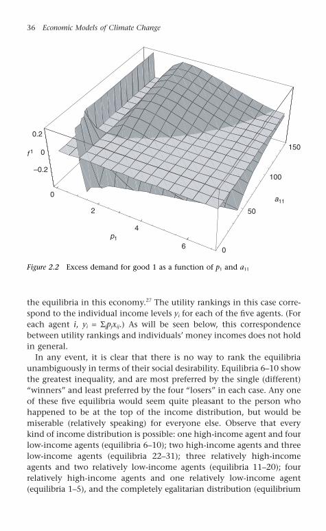
the equilibria in this economy.27 The utility rankings in this case corre-spond to the individual income levels yi for each of the five agents. (Foreach agent i, yi = Sjpjxij.) As will be seen below, this correspondencebetween utility rankings and individuals’ money incomes does not holdin general.

In any event, it is clear that there is no way to rank the equilibriaunambiguously in terms of their social desirability. Equilibria 6–10 showthe greatest inequality, and are most preferred by the single (different)“winners” and least preferred by the four “losers” in each case. Any oneof these five equilibria would seem quite pleasant to the person whohappened to be at the top of the income distribution, but would be miserable (relatively speaking) for everyone else. Observe that everykind of income distribution is possible: one high-income agent and fourlow-income agents (equilibria 6–10); two high-income agents and threelow-income agents (equilibria 22–31); three relatively high-incomeagents and two relatively low-income agents (equilibria 11–20); four relatively high-income agents and one relatively low-income agent(equilibria 1–5), and the completely egalitarian distribution (equilibrium


0

2

4

6p1

0

50

100

150

a11

–0.2

0

0.2

f 1

Figure 2.2 Excess demand for good 1 as a function of p1 and a11

1403_963363_03_cha02.qxd 6/14/2003 11:16 AM Page 36

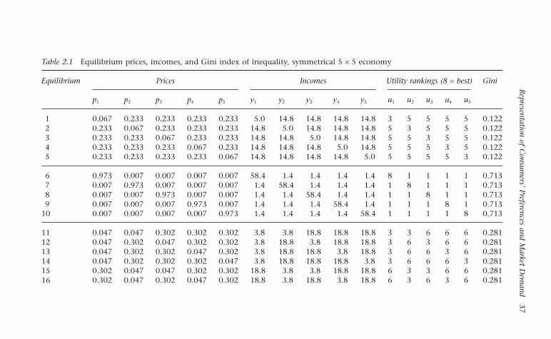
Representation of C

onsumers’ Preferences and M

arket Dem

and37

Table 2.1 Equilibrium prices, incomes, and Gini index of inequality, symmetrical 5 ¥ 5 economy

Equilibrium Prices Incomes Utility rankings (8 = best) Gini

p1 p2 p3 p4 p5 y1 y2 y3 y4 y5 u1 u2 u3 u4 u5

1 0.067 0.233 0.233 0.233 0.233 5.0 14.8 14.8 14.8 14.8 3 5 5 5 5 0.1222 0.233 0.067 0.233 0.233 0.233 14.8 5.0 14.8 14.8 14.8 5 3 5 5 5 0.1223 0.233 0.233 0.067 0.233 0.233 14.8 14.8 5.0 14.8 14.8 5 5 3 5 5 0.1224 0.233 0.233 0.233 0.067 0.233 14.8 14.8 14.8 5.0 14.8 5 5 5 3 5 0.1225 0.233 0.233 0.233 0.233 0.067 14.8 14.8 14.8 14.8 5.0 5 5 5 5 3 0.122

6 0.973 0.007 0.007 0.007 0.007 58.4 1.4 1.4 1.4 1.4 8 1 1 1 1 0.7137 0.007 0.973 0.007 0.007 0.007 1.4 58.4 1.4 1.4 1.4 1 8 1 1 1 0.7138 0.007 0.007 0.973 0.007 0.007 1.4 1.4 58.4 1.4 1.4 1 1 8 1 1 0.7139 0.007 0.007 0.007 0.973 0.007 1.4 1.4 1.4 58.4 1.4 1 1 1 8 1 0.713

10 0.007 0.007 0.007 0.007 0.973 1.4 1.4 1.4 1.4 58.4 1 1 1 1 8 0.713

11 0.047 0.047 0.302 0.302 0.302 3.8 3.8 18.8 18.8 18.8 3 3 6 6 6 0.28112 0.047 0.302 0.047 0.302 0.302 3.8 18.8 3.8 18.8 18.8 3 6 3 6 6 0.28113 0.047 0.302 0.302 0.047 0.302 3.8 18.8 18.8 3.8 18.8 3 6 6 3 6 0.28114 0.047 0.302 0.302 0.302 0.047 3.8 18.8 18.8 18.8 3.8 3 6 6 6 3 0.28115 0.302 0.047 0.047 0.302 0.302 18.8 3.8 3.8 18.8 18.8 6 3 3 6 6 0.28116 0.302 0.047 0.302 0.047 0.302 18.8 3.8 18.8 3.8 18.8 6 3 6 3 6 0.281

1403_963363_03_cha02.qxd 6/14/2003 11:16 AM Page 37

38Econom

ic Models of C

limate C

hange

Table 2.1 Continued

Equilibrium Prices Incomes Utility rankings (8 = best) Gini


17 0.302 0.047 0.302 0.302 0.047 18.8 3.8 18.8 18.8 3.8 6 3 6 6 3 0.28118 0.302 0.302 0.047 0.047 0.302 18.8 18.8 3.8 3.8 18.8 6 6 3 3 6 0.28119 0.302 0.302 0.047 0.302 0.047 18.8 18.8 3.8 18.8 3.8 6 6 3 6 3 0.28120 0.302 0.302 0.302 0.047 0.047 18.8 18.8 18.8 3.8 3.8 6 6 6 3 3 0.281

21 0.200 0.200 0.200 0.200 0.200 12.8 12.8 12.8 12.8 12.8 4 4 4 4 4 0

22 0.464 0.464 0.024 0.024 0.024 28.4 28.4 2.4 2.4 2.4 7 7 2 2 2 0.48823 0.464 0.024 0.464 0.024 0.024 28.4 2.4 28.4 2.4 2.4 7 2 7 2 2 0.48824 0.464 0.024 0.024 0.464 0.024 28.4 2.4 2.4 28.4 2.4 7 2 2 7 2 0.48825 0.464 0.024 0.024 0.024 0.464 28.4 2.4 2.4 2.4 28.4 7 2 2 2 7 0.48826 0.024 0.464 0.464 0.024 0.024 2.4 28.4 28.4 2.4 2.4 2 7 7 2 2 0.48827 0.024 0.464 0.024 0.464 0.024 2.4 28.4 2.4 28.4 2.4 2 7 2 7 2 0.48828 0.024 0.464 0.024 0.024 0.464 2.4 28.4 2.4 2.4 28.4 2 7 2 2 7 0.48829 0.024 0.024 0.464 0.464 0.024 2.4 2.4 28.4 28.4 2.4 2 2 7 7 2 0.48830 0.024 0.024 0.464 0.024 0.464 2.4 2.4 28.4 2.4 28.4 2 2 7 2 7 0.48831 0.024 0.024 0.024 0.464 0.464 2.4 2.4 2.4 28.4 28.4 2 2 2 7 7 0.488

Source: See text.

1403_963363_03_cha02.qxd 6/14/2003 11:16 AM Page 38

21). The Gini coefficient of income inequality varies dramatically across the equilibria. The Gini index ranges from 0 for equilibrium 21(the perfectly egalitarian income distribution) to the highly inegalitar-ian income distribution of equilibria 6 through 10 (Gini of 0.713).28

Equilibria 22 through 31 have an intermediate degree of income in-equality, with a Gini index of 0.488. For comparison, from the end ofWorld War II through the early 1990s, the Gini coefficient for inequal-ity of household income in the United States has ranged from a low of0.348 in 1968 to a high of 0.429 in 1992 (Weinberg 1996).

Each of these equilibria is a Pareto optimum: no consumer could bemade better off without decreasing the utility of at least one other consumer. The fact that the first-order conditions hold at each of the equilibrium points guarantees this result.29 The multiplicity of Pareto optimal equilibrium points does not mean, however, that theconsumers would be indifferent between such points, nor does it implywhich equilibrium would result from decentralized economic decision-making. If the members of society could somehow “vote” on whichequilibrium they would prefer, any of the 10 equilibria (11–20) couldcommand a majority. This majority would not necessarily be stablepolitically, however. Every majority of three relatively well-off agentscorresponds to one of the equilibria 11–20. Any one of these majoritiesof three would be vulnerable to reshuffling, as one of the disadvantagedminority could offer part of his income as “side payments” to twomembers of the majority as an inducement for them to form a newmajority coalition including the previously disadvantaged individual.30

This kind of reshuffling is hypothetical, of course; there is no way thata society could even know about the existence and properties of all theequilibria, let alone devise a procedure for choosing among them.

The different equilibria arise because the individuals have preferencesthat differ, they have endowment patterns that differ, and the goods are different (i.e., they are not good substitutes for each other). The parameters of the utility functions are such that the individuals’demand functions exhibit strong wealth effects. For an individual well-endowed with a particular good, an increase in the price of that goodcan increase the individual’s wealth sufficiently to offset the “substitu-tion effect” that would tend to cause the individual to substitute othergoods for the one whose price has increased. Such wealth effects are not unknown even for nonenvironmental goods – perhaps the mostcommon illustration is the backward-bending labor supply curve (thecase in which a sufficient increase in the wage induces the worker towork less and consume more leisure).


1403_963363_03_cha02.qxd 6/14/2003 11:16 AM Page 39

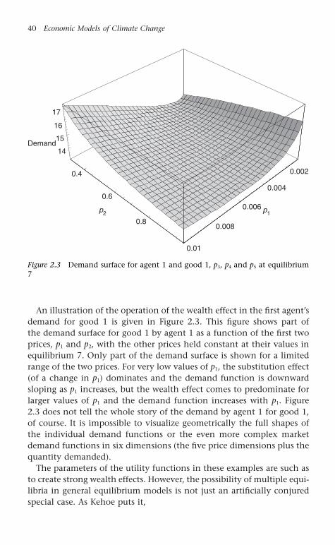
An illustration of the operation of the wealth effect in the first agent’sdemand for good 1 is given in Figure 2.3. This figure shows part of the demand surface for good 1 by agent 1 as a function of the first twoprices, p1 and p2, with the other prices held constant at their values inequilibrium 7. Only part of the demand surface is shown for a limitedrange of the two prices. For very low values of p1, the substitution effect(of a change in p1) dominates and the demand function is downwardsloping as p1 increases, but the wealth effect comes to predominate forlarger values of p1 and the demand function increases with p1. Figure2.3 does not tell the whole story of the demand by agent 1 for good 1,of course. It is impossible to visualize geometrically the full shapes ofthe individual demand functions or the even more complex marketdemand functions in six dimensions (the five price dimensions plus thequantity demanded).

The parameters of the utility functions in these examples are such asto create strong wealth effects. However, the possibility of multiple equi-libria in general equilibrium models is not just an artificially conjuredspecial case. As Kehoe puts it,


0.002

0.004

0.006

0.008

0.01

p1

0.4

0.6

0.8

p2

14

15

16

17

Demand

Figure 2.3 Demand surface for agent 1 and good 1, p3, p4 and p5 at equilibrium7

1403_963363_03_cha02.qxd 6/14/2003 11:16 AM Page 40

Non-uniqueness of equilibrium does not seem so pathological a situation as to warrant unqualified used of the simple comparativestatics method when dealing with general equilibrium models. . . .[F]or most of these models no method now exists to determinewhether the equilibrium found . . . is unique. To make matters worse,it appears that non-uniqueness of equilibria is an even more com-mon situation in applied models that allow for such distortions as taxes, price rigidities, and unemployment than it is in the simplemodel. . . . (1985, p. 145)

There is very little “lore” about the conditions under which the multi-plicity of equilibria arises in practical applications.31 It certainly is notpossible to examine the expenditure shares of the different goods in theeconomy and conclude from them that the ones with low shares in thetotal value of output are “less important” than those with high shares.In the model of Table 2.1, the expenditure shares of the different goods are the same as their relative prices because the endowments are completely symmetrical and the total quantity of each good is 64 units. But in equilibrium 6, for example, the expenditure share of good 1 is 97.3 percent, while the shares of goods 2 through 5 are 0.7percent each. Good 1 makes up the lion’s share of GDP, while goods 2,3, 4, and 5 each make up less than 1 percent of GDP. However, this isentirely a consequence of the fact that the economy happens to be inequilibrium 6; in equilibrium 7, good 2 has the overwhelming expen-diture share while the shares of the other goods are small. The expen-diture shares of the different goods vary across each of the 31 equilibria.Yet the utility functions and endowments are entirely symmetrical, so itwould be sensible to maintain that all the goods are equally “impor-tant.” If multiple equilibria exist, there is no way to infer the relativeimportance of the goods to individuals from the expenditure shares ofthe goods.

Some work has been done to explore the question of multiplicity inapplied models (see, for example, Kehoe and Whalley 1985), but evenif the computational burden were not formidable, checking existingmodels for multiple equilibria would not really address the problem.The reason is that the issue of multiple equilibria is often settled in the design of the models without reference to any underlying economicreality, and therefore is not an issue that can be explored by examina-tion of finished models. We will return to this issue below.

Now consider the same type of 5¥5 model economy, but with oneminor change. All the utility functions are the same as in the first


1403_963363_03_cha02.qxd 6/14/2003 11:16 AM Page 41

example, and all the endowments are the same with the exception that agent 1’s endowment of the first good is 70 rather than 60. Thiseconomy has at least 25 equilibria, as displayed in Table 2.2.

Table 2.2 is similar to Table 2.1 in that the agents’ utility rankings cor-respond to their income levels. Unlike in the previous model, however,the GDP is not the same in all the equilibria. Because agent 1 has aslightly larger endowment, the GDP values computed for the entireeconomy follow the same ranking as the utility ranking for agent 1. Thissurely does not correspond to any kind of “social” ranking of the equi-libria however; it is evident from Table 2.2 that four out of the fiveagents making up the economy would prefer any equilibrium (with theexception of 12–15) to equilibrium 11, the one having the highest GDP.(These relative rankings are independent of the price normalization rule,again because the relative prices are not dependent on the normaliza-tion rule chosen.) As in Table 2.1, if the agents could vote on whichequilibrium the economy should reach, a majority could be put togetherthat would support one of the set from 16 through 19, although the“divide the pie” type of political instability discussed before makes itimpossible to determine a particular majority-preferred equilibriumwithin that set. The GDP of these equilibria are in fact the third-lowestof the possibilities, because agent 1 fares poorly. The voting rules matteras well. If a supermajority of four votes were required for the society topick an equilibrium, it would settle on equilibrium 1, which has a higher GDP than any of the set 16–19 that would be reached by simplemajority rule.

A third example 5 ¥ 5 model differs from the first two in that the con-sumers have different elasticities of substitution, as well as differentendowments. As in the first two examples, there are five consumers and five goods. The weights in the consumers’ utility functions are thesame as before, but now b1 = -3, b2 = -3, b3 = -4, b4 = -5, and b5 = -5.The endowments are given by w11 = w55 = 70, w22 = w33 = w44 = 60, andwij = 1 (i π j, "i, j). This third example also exhibits multiple equilibria.The consumers’ utility functions are not symmetric, so the equilibriawill not fall into symmetrical groups as did many of the equilibria inTables 2.1 and 2.2. At the same time, because the numerical search forequilibria is sensitive to the starting point (and possibly also to thenumerical search method), there is no guarantee that all the equilibriaare displayed in Table 2.3.32 The table contains the values for prices,incomes, and utility rankings for five equilibria that were found,however. As in the case of Table 2.2, the ranking of equilibria by GDPtells us nothing about the social desirability of the equilibria. The GDP


1403_963363_03_cha02.qxd 6/14/2003 11:16 AM Page 42

Representation of C


arket Dem

and43

Table 2.2 Equilibrium prices, incomes, and utility rankings, 5 ¥ 5 economy, asymmetrical endowments

Equilibrium Prices Incomes Utility rankings (8 = best GDPfor agent 1, 13 = best for

p1 p2 p3 p4 p5 y1 y2 y3 y4 y5 agents 2–5)

u1 u2 u3 u4 u5

1 0.017 0.246 0.246 0.246 0.246 2.2 15.5 15.5 15.5 15.5 4 10 10 10 10 64.1693

2 0.553 0.149 0.099 0.099 0.099 39.1 9.8 6.9 6.9 6.9 6 8 6 6 6 69.52903 0.553 0.099 0.149 0.099 0.099 39.1 6.9 9.8 6.9 6.9 6 6 8 6 6 69.52904 0.553 0.099 0.099 0.149 0.099 39.1 6.9 6.9 9.8 6.9 6 6 6 8 6 69.52905 0.553 0.099 0.099 0.099 0.149 39.1 6.9 6.9 6.9 9.8 6 6 6 6 8 69.5290

6 0.594 0.216 0.063 0.063 0.063 42.0 13.7 4.7 4.7 4.7 7 9 5 5 5 69.94057 0.594 0.063 0.216 0.063 0.063 42.0 4.7 13.7 4.7 4.7 7 5 9 5 5 69.94058 0.594 0.063 0.063 0.216 0.063 42.0 4.7 4.7 13.7 4.7 7 5 5 9 5 69.94059 0.594 0.063 0.063 0.063 0.216 42.0 4.7 4.7 4.7 13.7 7 5 5 5 9 69.9405

10 0.549 0.113 0.113 0.113 0.113 38.9 7.7 7.7 7.7 7.7 5 7 7 7 7 69.4866

11 0.937 0.016 0.016 0.016 0.016 65.7 1.9 1.9 1.9 1.9 8 2 2 2 2 73.3732

12 0.003 0.978 0.007 0.007 0.007 1.2 58.7 1.4 1.4 1.4 1 13 1 1 1 64.0287

1403_963363_03_cha02.qxd 6/14/2003 11:16 AM Page 43

44Econom

ic Models of C

limate C

hange

Table 2.2 Continued

Equilibrium Prices Incomes Utility rankings (8 = best GDPfor agent 1, 13 = best for

p1 p2 p3 p4 p5 y1 y2 y3 y4 y5 agents 2–5)

u1 u2 u3 u4 u5

13 0.003 0.007 0.978 0.007 0.007 1.2 1.4 58.7 1.4 1.4 1 1 13 1 1 64.028714 0.003 0.007 0.007 0.978 0.007 1.2 1.4 1.4 58.7 1.4 1 1 1 13 1 64.028715 0.003 0.007 0.007 0.007 0.978 1.2 1.4 1.4 1.4 58.7 1 1 1 1 13 64.0287

16 0.014 0.043 0.314 0.314 0.314 2.0 3.5 19.6 19.6 19.6 3 4 11 11 11 64.137917 0.014 0.314 0.043 0.314 0.314 2.0 19.6 3.5 19.6 19.6 3 11 4 11 11 64.137918 0.014 0.314 0.314 0.043 0.314 2.0 19.6 19.6 3.5 19.6 3 11 11 4 11 64.137919 0.014 0.314 0.314 0.314 0.043 2.0 19.6 19.6 19.6 3.5 3 11 11 11 4 64.1379

20 0.009 0.473 0.473 0.022 0.022 1.6 28.9 28.9 2.3 2.3 2 12 12 3 3 64.085521 0.009 0.473 0.022 0.473 0.022 1.6 28.9 2.3 28.9 2.3 2 12 3 12 3 64.085522 0.009 0.473 0.022 0.022 0.473 1.6 28.9 2.3 2.3 28.9 2 12 3 3 12 64.085523 0.009 0.022 0.473 0.473 0.022 1.6 2.3 28.9 28.9 2.3 2 3 12 12 3 64.085524 0.009 0.022 0.473 0.022 0.473 1.6 2.3 28.9 2.3 28.9 2 3 12 3 12 64.085525 0.009 0.022 0.022 0.473 0.473 1.6 2.3 2.3 28.9 28.9 2 3 3 12 12 64.0855

Source: See text. Values for agent 1 are italicized to indicate that this agent’s endowment is different from that of the other agents.

1403_963363_03_cha02.qxd 6/14/2003 11:16 AM Page 44

Representation of C


arket Dem

and45

Table 2.3 Equilibrium prices, incomes, and utility rankings, 5 ¥ 5 economy, asymmetrical endowments and unequal substitutionelasticities

Equilibrium Prices Incomes Utility rankings (5 = best) GDP


1 0.692 0.275 0.016 0.012 0.006 48.7 17.2 1.9 1.7 1.4 4 4 3 5 5 71.02 0.962 0.020 0.009 0.006 0.003 67.4 2.2 1.5 1.4 1.2 5 1 2 3 4 73.73 0.005 0.985 0.005 0.003 0.002 1.3 59.1 1.3 1.2 1.1 1 5 1 1 1 64.074 0.007 0.021 0.963 0.005 0.003 1.5 2.3 57.8 1.3 1.2 2 2 5 2 2 64.105 0.011 0.159 0.816 0.009 0.004 1.8 10.4 49.1 1.6 1.3 3 3 4 4 3 64.2. . . . . . . . . . . . . . . . .. . . . . . . . . . . . . . . . .. . . . . . . . . . . . . . . . .? . . . . . . . . . . . . . . . .

Source: See text.

1403_963363_03_cha02.qxd 6/14/2003 11:16 AM Page 45


associated with equilibrium 2 is highest, yet a majority (in fact, all butagent 1) would prefer equilibrium 1 over equilibrium 2. As in the pre-vious cases, some of these equilibria are characterized by a highlyunequal distribution of income; this results when the price of one par-ticular good is considerably higher than the price of the other goods.(If an individual is endowed with a disproportionately large share of ahigh-priced good, that individual’s income will be disproportionatelyhigh in the equilibrium.) The model differs from the other two in thatan agent’s personal income does not give an unambiguous indicationof the individual’s utility ranking of an equilibrium. Agent 5’s incomeis higher in equilibrium 5 than in equilibrium 2, yet this agent’s utilityis greater in equilibrium 2.

Different multiple equilibria can arise under other variations in specification of the model. As the parameters and endowments vary,there can be different numbers of equilibria.33 For some ranges of theparameters the equilibrium is unique, although a full search of the parameter space to find the region having a unique equilibrium isimpractical even in the case of these very simple 5¥5 models. Thedimensionality of the problem is just too large. With n commodities,each agent would require specification of n - 1 utility weights aij

(each agent’s utility function can be rescaled to make ai1 = 1), one substitutability parameter bi, and n endowments wij, or 2n parametersin all. Thus, with n agents and n goods the full parameter space wouldhave n ¥ (2n) = 2n2 parameters. Defining the commodity units by settingthe wij for one agent all equal to one would reduce the number of parameters to 2n2 - n. If the substitution parameters differed acrossgoods for each consumer (so that there were n of the b’s for each consumer), the total number of parameters would be 3n2 - 2n. Thus,the number of parameters increases quadratically with the size of theeconomy. The ranges of these parameters are bounded from only oneside – the aij’s can be presumed to be positive, the bi’s less than one, andthe wij’s greater than zero – so there is no way to search the parameterspace over a finite grid. And this is for only a simple exchange economy;the number of parameters increases even more if production were to beintroduced.

2.3.2 The unknown dynamics of the general equilibrium system

The equilibrium prices and incomes shown in Tables 2.1–2.3 were calculated using numerical routines for solving a simultaneous systemof nonlinear equations.34 This does not mean that a real economy would

1403_963363_03_cha02.qxd 6/14/2003 11:16 AM Page 46

be able to find or would converge to any of these equilibria; that woulddepend on the actual dynamics of the economic system. Economistshave shied away from incorporating dynamic adjustment mechanismsinto their integrated assessment models for good reasons.35 If transac-tions are allowed to take place “out of equilibrium,” the model wouldhave to deal with the possibility of shortages and surpluses – and theplans of consumers and producers would not be fulfilled. Nonfulfill-ment of plans means that the maximization that presumably definesthe behavior of the producers and consumers is incomplete. This woulddestroy any favorable welfare interpretation of the prices and transactedquantities observed in the markets. But the theoretical difficulties rundeeper; transactions “out of equilibrium” would also affect the wealthof the agents, and would therefore change the conditions for their max-imization subsequently in unforeseeable ways (Fisher 1983, 1989).36 Onthe other hand, if out of equilibrium transactions are to be avoided,there must be some mechanism for arriving at the equilibrium pricesprior to any transactions taking place. Obviously, no such economy-wide mechanism exists.

This lack of a well-defined equilibrium-finding mechanism has beenan embarrassment since the earliest days of mathematical economicsand general equilibrium theory. The most familiar way out is the tâton-nement (“groping”) process of the type originally hypothesized byWalras. In the tâtonnement, it is imagined that prices adjust accordingto excess demands – if there is positive excess demand for a commod-ity, its price increases, while if excess demand is negative, the pricedecreases.37 In elementary treatments, something like the adjustmentprocess situation depicted in Figure 2.4 is presumed to be taking place.

Figure 2.4 represents a particular market, say for automobiles. Thedemand and supply curves are shown as depending on the price of auto-mobiles (although note that in the background, the level of income ofconsumers is an important determinant of demand). If for any particu-lar price of automobiles P0, the amount that auto manufacturers wouldlike to sell (given by the supply curve) is greater than the amount consumers want to buy (indicated by the demand curve), there will be excess supply. This could manifest itself as a buildup of inventories,or a slowdown in the rate of sales from what is “normal.” Faced withthese conditions, suppliers would cut prices with the aim of workingdown the inventories and stimulating demand. Similarly, if P0¢ were “toolow” (i.e., below equilibrium) consumers would want to buy more carsthan producers were willing to sell, and the situation would be one of


1403_963363_03_cha02.qxd 6/14/2003 11:16 AM Page 47

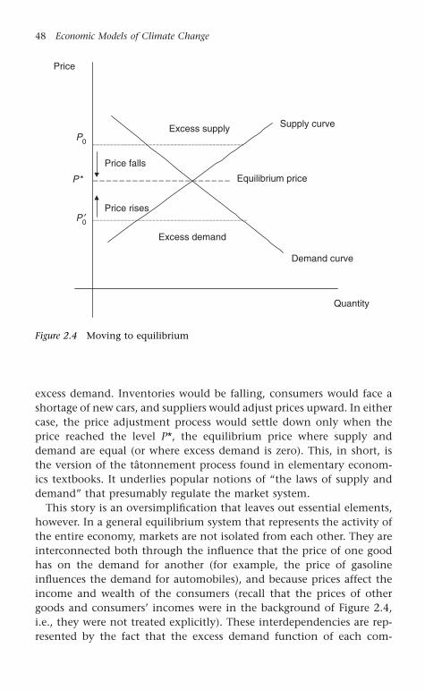
excess demand. Inventories would be falling, consumers would face ashortage of new cars, and suppliers would adjust prices upward. In eithercase, the price adjustment process would settle down only when theprice reached the level P*, the equilibrium price where supply anddemand are equal (or where excess demand is zero). This, in short, isthe version of the tâtonnement process found in elementary econom-ics textbooks. It underlies popular notions of “the laws of supply anddemand” that presumably regulate the market system.

This story is an oversimplification that leaves out essential elements,however. In a general equilibrium system that represents the activity ofthe entire economy, markets are not isolated from each other. They areinterconnected both through the influence that the price of one goodhas on the demand for another (for example, the price of gasoline influences the demand for automobiles), and because prices affect theincome and wealth of the consumers (recall that the prices of othergoods and consumers’ incomes were in the background of Figure 2.4,i.e., they were not treated explicitly). These interdependencies are rep-resented by the fact that the excess demand function of each com-


Excess supplyP0

Price falls

P0

Price rises

Excess demand

P * Equilibrium price

Quantity

Price

Supply curve

Demand curve

¢

Figure 2.4 Moving to equilibrium

1403_963363_03_cha02.qxd 6/14/2003 11:16 AM Page 48

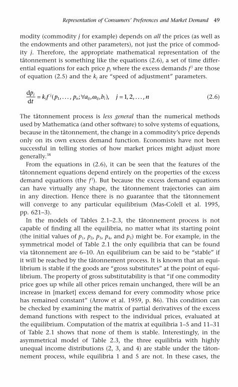
modity (commodity j for example) depends on all the prices (as well asthe endowments and other parameters), not just the price of commod-ity j. Therefore, the appropriate mathematical representation of thetâtonnement is something like the equations (2.6), a set of time differ-ential equations for each price pj where the excess demands f j are thoseof equation (2.5) and the kj are “speed of adjustment” parameters.

(2.6)

The tâtonnement process is less general than the numerical methodsused by Mathematica (and other software) to solve systems of equations,because in the tâtonnement, the change in a commodity’s price dependsonly on its own excess demand function. Economists have not beensuccessful in telling stories of how market prices might adjust more generally.38

From the equations in (2.6), it can be seen that the features of thetâtonnement equations depend entirely on the properties of the excessdemand equations (the f j). But because the excess demand equationscan have virtually any shape, the tâtonnement trajectories can aim in any direction. Hence there is no guarantee that the tâtonnement will converge to any particular equilibrium (Mas-Colell et al. 1995, pp. 621–3).

In the models of Tables 2.1–2.3, the tâtonnement process is notcapable of finding all the equilibria, no matter what its starting point(the initial values of p1, p2, p3, p4, and p5) might be. For example, in thesymmetrical model of Table 2.1 the only equilibria that can be foundvia tâtonnement are 6–10. An equilibrium can be said to be “stable” ifit will be reached by the tâtonnement process. It is known that an equi-librium is stable if the goods are “gross substitutes” at the point of equi-librium. The property of gross substitutability is that “if one commodityprice goes up while all other prices remain unchanged, there will be anincrease in [market] excess demand for every commodity whose pricehas remained constant” (Arrow et al. 1959, p. 86). This condition canbe checked by examining the matrix of partial derivatives of the excessdemand functions with respect to the individual prices, evaluated at the equilibrium. Computation of the matrix at equilibria 1–5 and 11–31of Table 2.1 shows that none of them is stable. Interestingly, in theasymmetrical model of Table 2.3, the three equilibria with highlyunequal income distributions (2, 3, and 4) are stable under the tâton-nement process, while equilibria 1 and 5 are not. In these cases, the

ddpt

k f p p a b j njj

jn ij ij i= "( ) =1 1 2, . . . , ; , , , , , . . . ,w


1403_963363_03_cha02.qxd 6/14/2003 11:16 AM Page 49

stable equilibria are those which are best for a single agent, and worstfor everyone else.

Knowledge of the dynamics of the economic system is, nevertheless,an essential component of understanding how the system would reactto any kind of shock, including a policy change. It was proved byDebreu (1970) that economies of the type being considered here are“regular.”39 What happens if a “regular” economy is perturbed from one of its finite number of equilibria? The dynamic path followed bythe economy will determine whether it returns to that equilibrium orto another one. Some kinds of dynamics might not enable the economyto reach equilibria that might be, on social or political grounds, desir-able. The actual outcome of any “comparative statics” exercise involv-ing a policy change or parametric shock will also depend on the realdynamics of the economy. Given the possibility of multiple equilibria, aneconomic model, to be useful for policy analysis purposes, must includea specification of economic dynamics.

2.3.3 Can current models reveal multiple equlibria and unstable dynamics?

In the empirical implementation of general equilibrium modeling, thereare several ways to arrive at the representation of consumers and their preferences. The first is to specify market demand functions andestimate them from aggregate data, relying on the interaction of thesedemand functions and production-based supply functions (perhaps alsoestimated from aggregate data) to determine prices and outputs in thegeneral equilibrium solution of the model. Often, these market demandfunctions are presumed to represent the demand of a “representativeconsumer” or consumers who exhibit the same characteristics as realindividuals. A second approach is to start with a specification of theconsumers’ utility functions, and to estimate a “demand system” basedon price and expenditure data. The market demand equations wouldthen be built up by summing the individuals’ demand functions. A thirdapproach is to specify demand functions a priori, sometimes relying onstudies in the literature to provide values of the relevant parameters.The functions may be calibrated to aggregate data, or some com-bination of calibration and econometric estimation may be used. Inpractice, each of these methods has drawbacks. None offers a fully satisfactory answer to the question of whether or not multiple equilib-ria are possible.


1403_963363_03_cha02.qxd 6/14/2003 11:16 AM Page 50

Consider first the specification of market demand functions based onthe “representative agent” approach. It has been observed by no less anauthority than James Tobin that an economics paper that does not beginwith rational maximization by representative agents (i.e., that is notbased on “microfoundations”) would be unlikely to see the light of day:

[The microfoundations] counter-revolution has swept the professionuntil now it is scarcely an exaggeration to say that no paper that doesnot employ the “microfoundations” methodology can get publishedin a major professional journal, that no research proposal that issuspect of violating its precept can survive peer review, that no newlyminted Ph.D. who can’t show that his hypothesized behavioral rela-tions are properly derived can get a good academic job.

(Tobin 1986, quoted in Rizvi 1994, p. 350)

It is hard to understand why this self-imposed methodological con-straint is so uniformly upheld. It has been known for some time thatthe representative agent approach is fundamentally inconsistent. Thereason is that if a representative agent is constructed on the basis thatthis agent reproduces market outcomes, the implied preferences of therepresentative agent can be in conflict with the actual preferences of theagents making up the economy (Jerison 1984, cited in Kirman 1992).The representative agent may prefer commodity bundle A to bundle Bat some set of prices, even though the individual agents in the economyall prefer B to A. Once again, individual demands do not aggregate toa market demand of the same form. Kirman’s appraisal is telling:

A tentative conclusion, at this point, would be that the representativeagent approach is fatally flawed because it attempts to impose orderon the economy through the concept of an omniscient individual. In reality, individuals operate in very small subsets of the economyand interact with those with whom they have dealings. . . .

(1992, p. 132)

Kirman goes on to describe some promising attempts that have beenmade to show how systematic outcomes could result from such local-ized interactions, but he concludes that

[t]he equilibria of the worlds described by any of these approachesmay be conceptually very different from those implied by the


1403_963363_03_cha02.qxd 6/14/2003 11:16 AM Page 51

artifact of the representative individual. . . . In a world with manyinteracting heterogeneous agents, a natural idea of an equilibriumwould be not a particular state, but rather a distribution over states,reflecting the proportion of time the economy spends in each of the states. This distribution could exhibit very regular character-istics, while remaining far from reflecting the behavior of a singlemaximizing agent.

(1992, p. 133, footnote and references omitted)

Kirman’s judgment at the beginning of his review is a fair summary:“[T]he ‘representative’ agent deserves a decent burial, as an approach to economic analysis that is not only primitive, but fundamentally erroneous” (1992, p. 119).

Building up aggregate demand functions out of demand systems esti-mated from individual expenditure data also faces difficulties. If impor-tant elements of the utility function, such as the environment, are notpriced, then in practice no data on consumer expenditures can revealthe parameters of the utility function that are associated with that“commodity.” This is precisely the situation with regard to climate sta-bility and other desirable attributes of the global environment.40 Evenfor the commodities that are traded in markets, severe dimensionalityproblems prevent the recovery of all of the parameters of the consumers’utility functions. Flexible functional forms derived as Taylor seriesapproximations of general utility functions have a number of param-eters that increases quadratically with the number of goods. The datarequirements for estimating such a demand system are formidable, andas a result such systems are typically estimated only after a number ofrestrictive assumptions are made that drastically reduce the number offree parameters. Examples of such restrictions include specifying thatsome of the parameters are the same across all consumers, or that certainelasticities are known a priori. This brings us back to the problems asso-ciated with positing a “representative consumer” and with limiting thepotential complementarity of goods.

The third alternative is simply to rely on aggregate statistical infor-mation to estimate market demand and supply curves for the variouscommodities traded in the economy. Such a rough-and-ready approachhas some appeal, except that the results of the estimation procedurecannot then be used to make welfare arguments. If the empirical de-mand and supply curves are robust under alternative policy scenarios(this is itself a questionable assumption), then the empirically based estimates might have some predictive value. However, hypothetical


1403_963363_03_cha02.qxd 6/14/2003 11:16 AM Page 52

changes in market aggregates calculated on the basis of such a model(such as changes in GDP or prices) would have no normative implica-tions, because they could not be mapped to changes in the circum-stances or preferences of individuals.

Another very serious problem with atheoretical estimates has to do with specification of their functional forms for estimation. We know from the Sonnenschein–Mantel–Debreu theorem that the mar-ket demand functions can have almost any shape. If so, what func-tional forms would be appropriate for estimation of those functionsbased on market data? It would not be possible to appeal to the theoryof the individual consumer for restrictions; the point of the theoreticalresults is that the aggregate demand functions do not necessarilyhave the same properties as individual demand functions. Yet somerestrictions are necessary both to identify the functions (Fisher 1966)and to produce sufficient degrees of freedom for statistical estimation.It is difficult to imagine a credible procedure for atheoretical estimationin the face of fundamental indeterminacy of the underlying functionalforms.

Most common in the practice of integrated assessment is to assumethat the utility functions of the consumers take on some highly sim-plified form. Usually representative consumers are specified; the param-eters are selected by the analyst (with perhaps some reference toempirical work). Collapsing preferences into this kind of representationrules out by assumption the problems of multiple equilibria and insta-bility if the posited utility functions impose a high degree of substi-tutability on the different goods (or if the differences in goods are simplyassumed away and utility is specified to depend on aggregate GDP). Forexample, the Cobb–Douglas utility function implies that the elasticityof substitution between all goods is unity. It amounts to imposing grosssubstitutability (which, in exchange models, implies uniqueness of equilibrium and tâtonnement stability) by assumption.

To provide a flavor of the current “state of the art” in integrated assess-ment modeling, consider the sample of models that participated in therecent Energy Modeling Forum evaluation of the “costs of Kyoto.” Aspecial issue of the Energy Journal compiled the results of the runs of 13models, along with descriptions of the scenarios that were simulated.The modelers gave summary descriptions of their models and how they implemented the scenarios. How are consumers’ preferences rep-resented in these models?

Table 2.4 shows how each model does it. Recall that logarithmic util-ity functions are the same as Cobb–Douglas, because any monotonic


1403_963363_03_cha02.qxd 6/14/2003 11:16 AM Page 53


Table 2.4 Representation of preferences in integrated assessment models

Model Representative Intraperiod Interperiodconsumers (for functional form functional formregions) of utility function of utility function

MERGEa yes logarithmic discounted sumSGMb yes demandb demandb

EPPAc yes Cobb–Douglas single–periodRICEd yes logarithmic discounted sumFUNDe yes adjusted log discounted sumGRAPEf yes logarithmicf discounted sumWorldScang yes Cobb–Douglasg discounted sumg

AIMh yesh –h –h

MS-MRTi yes Cobb–Douglasi discounted sum CESi

GTEMj yes CDEj single-periodj

G-Cubedk yes Cobb–Douglask discounted sum logOxfordl – – –CETA-Mm yes logarithmic discounted sum

Notes: The papers in the special issue of The Energy Journal are Manne and Richels (1999),MacCracken et al. (1999), Jacoby and Wing (1999), Nordhaus and Boyer (1999), Tol(1999), Kurosawa et al. (1999), Bollen et al. (1999), Kainuma et al. (1999), Bernstein et al.(1999b), Tulpulé et al. (1999), McKibbin et al. (1999), Cooper et al. (1999), and Peck andTeisberg (1999).a MERGE: “Global Negishi welfare is a weighted sum of the discounted logarithm ofmacroeconomic consumption, adjusted for the economic losses generated by non-marketdamages. . . . In the Pareto-optimal case, nonmarket damages enter the Negishi welfaredefinition, and market damages represent one of the competing claims on the allocationof total production resources. In all other cases, nonmarket and market damages areexcluded from the determination of the equilibrium, but are determined in a post-optimization step. In this way, we allow for the possibility of non-cooperation or of non-optimal international control agreements.” (For further discussion, see the websitehttp://www.stanford.edu/group/MERGE/.)b SGM: There are four final demand sectors (personal consumption, governmentconsumption, investment, and net exports). Household utility functions are not defined;instead, household demand for each final product is specified as a normalized demandfunction with a price and income elasticity. The household supplies of labor and savingsare also modeled as supply functions and are not derived from underlying utilityfunctions. Government utility is CES in general government services, national defense,and education (Sands et al. 1999).c EPPA: The representative agent in each region for each period maximizes U = Pc (Yc - qc)mc

for the four consumption goods indexed by c, with Yc equal to consumption and qc aminimum consumption level (Yang et al. 1996). This modified Cobb–Douglas utility function is also referred to as a “linear expenditure system.” Utility is maximized in eachperiod, and “[f]actor endowments are updated at each step, according to assumed exogenous trends in rates of population growth, increases in labor productivity,autonomous energy efficiency improvement (AEEI), and availability of natural resources”(Jacoby and Wing 1999, p. 77, citing Yang et al. 1996).

1403_963363_03_cha02.qxd 6/14/2003 11:16 AM Page 54


Notes to Table 2.4 continued

d RICE: The RICE model notionally specifies an additively separable (for each time period)CES utility function with consumption per capita in each period as the arguments, butwhen it comes to carrying out the actual runs of the model, the substitution parameter ischosen so as to make the utility function logarithmic (Nordhaus and Boyer 2000).e FUND: Utility is the logarithm of per capita consumption minus investment minusmarket damages, plus a second-order Taylor approximation for monetized nonmarketdamages. The Taylor approximation is used because “in some uncertainty analyses somany people died that the non-market losses exceed income” (Tol, personalcommunication, 2001).f GRAPE: A single utility function consisting of a weighted (with Negishi weights) sum ofthe individual regions’ utilities functions is maximized.g WorldScan: Intertemporal optimization by the representative agents maximizes the dis-counted sum of the logarithm of annual consumption, where the discount rate includesthe probability that the consumer will be alive in the next period. The instantaneousutility functions are Cobb–Douglas in the seven categories of goods. Demand for a particular category within a region is a CES composite of all varieties produced in the different regions (CPB Netherlands Bureau of Economic Policy Analysis 1999).h AIM: Model structure not accessible.i MS-MRT: The nonenergy goods enter the intraperiod utility function in Cobb–Douglasform, but end-use energy consumption enters the utility function directly in CES formwith the aggregate of nonenergy goods. The intertemporal sum that is maximized is aseparable utility function with a constant elasticity of intertemporal substitution. Importsfrom different regions and domestically produced goods are distinguished (Bernstein et al.1999b).j GTEM: The commodities include coal, oil, and natural gas. Intraperiod utility functionsare of the “constant difference elasticity” (CDE) type (Hanoch 1975). Income in a givenperiod is divided between savings and consumption in fixes proportions according to alife-cycle model and demographic representation of the composition of the population.Additional dynamic equations represent adjustment of stock variables (ABARE 2002).k G-Cubed: The intertemporal utility function that is maximized is of the form

where C(s) is the household’s aggregate consumption of goods at time s, G(s) isgovernment consumption, and q is the rate of time preference (set equal to 2.5%). Thefinal consumption function is modified to account for deviations from the permanentincome hypothesis. Within each period, C(s) is treated as a nested CES function; the toptier consists of inputs of capital services, labor, energy, and materials; energy and materialsare CES aggregates of inputs of individual goods. “The elasticities of substitution at theenergy and materials tiers were estimated to be 0.8 and 1.0, respectively. In this version of the model the top tier elasticity has been imposed to be unity” (McKibbin et al. 1999,pp. 295–6). Thus, at all levels of the utility function except the energy aggregate, thespecification is Cobb–Douglas (elasticity of substitution of unity).l The Oxford model is not a general equilibrium model and does not contain an explicitrepresentation of preferences.m CETA-M: Market and nonmarket damages monetized. See Peck and Teisberg (1992) forspecification of the utility function.

U C s G s sts t

t= ( ) + ( )[ ] - -( )

•

Ú ln ln e dq

1403_963363_03_cha02.qxd 6/14/2003 11:16 AM Page 55


transformation of a utility function has the same observable impli-cations as the original utility function. Thus, we can see that in all butone of the models participating in EMF-16, either the intraperiod utilityfunctions were Cobb–Douglas and did not include environmental goods,or the value of environmental goods was simply monetized. In the lattercase, of course, the implicit elasticity of substitution between the envi-ronmental goods and other goods is infinite – they are perfectly substi-tutable at the prices chosen for the monetization. For Cobb–Douglasutility functions defined over ordinary goods, the market demand functions are linear in normalized (or relative) prices, and hence theequilibrium necessarily is unique. Specification of Cobb–Douglas (orlogarithmic) utility rules out by assumption the possibility of multipleequilibria originating on the demand side. In all but one of the models,the intertemporal substitutability of the goods was also high by defini-tion. The implications of that assumption will be treated in the follow-ing chapter.

2.4 Conclusions and implications for policy

What can we conclude from this review of the treatment of preferencesin integrated assessment models? It is clear that the existing models areset up in such a way as to preclude any of the problems with multi-plicity of equilibria or instability of equilibria arising from the demandside. This is not to say that the real world does in fact exhibit multi-plicity of equilibria and instability; that is a question that remains to bedetermined. A great deal of empirical work would be required, especiallybecause the representation of nonmarketed environmental goods inindividual preferences is a subject that is largely unexplored.

The inadequacies of the representation of consumers in standard economic climate policy models can therefore be summarized asfollows:

• The “outside” critique of preference representation is entirelyignored;

• For intraperiod utility, the diversity of individual consumers withineach region of analysis (typically a large country such as the US orChina, or a multicountry region such as the EU) is replaced by a representative agent, even though it is known that the representa-tive agent assumption is not adequate to capture the actual shape ofmarket demand functions;

• Either environmental goods are left out of the utility function, or

1403_963363_03_cha02.qxd 6/14/2003 11:16 AM Page 56

their contribution to well-being is simply monetized, thereby precluding investigation of any questions having to do with thepotential complementarity of environmental and nonenvironmen-tal goods. If environmental goods are monetized (as in conventionalCBA), the implicit assumption is that the elasticity of substitution fornonmarginal changes in the composition of environmental andnonenvironmental goods in utility is infinite;

• The preferences of the representative agents are typically describedby logarithmic or Cobb–Douglas utility functions, thereby imposinggross substitutability. Multiple or unstable equilibria arising out ofthe properties of consumers’ demand functions are thereby ruled out.

Current specimens of climate/economy applied general equilibriummodels thus are incapable of revealing multiple equilibria, even if the realeconomy has them. The project of establishing such models on “micro-foundations” is not a movement in the direction of greater rigor;instead, it creates the erroneous impression that modeling conclusionshave been derived from unassailable scientific procedures, when in factthe results are no more than the consequences of the assumptions builtinto the models. Very strong (and entirely untested) assumptions arerequired to rule out the possibilities of multiple equilibria and dynamicinstability. In reality, the true number of equilibria in the real economyis not known. Nor is very much known about the actual process of dynamic adjustment within the economy. What is known is thateven elementary general equilibrium systems can exhibit diverse andproblematic phenomena. The multiple equilibria of the simple ex-change models discussed here should give pause to those who wouldunquestioningly accept the results of the current generation of morecomplicated integrated assessment models.


1403_963363_03_cha02.qxd 6/14/2003 11:16 AM Page 57

3The Treatment of Time

58

3.1 The problem

Climate change takes place over decades, centuries, and millennia. Theconsequences of actions taken now also work themselves out on timescales covering multiple generations. The persistence of CO2 in theatmosphere depends on the long-term response of the biosphere toincreased temperatures and concentrations, and the atmospheric life-times of many of the non-CO2 greenhouse gases are over 100 years. Theachievement of thermal equilibrium between the surface layers of theocean and atmosphere takes decades, and achievement of equilibriumbetween the different layers of the ocean requires even more time (IPCC2001a).1 These physical facts mean that the treatment of events andpolicies that unfold over very long stretches of time must be a centralfeature of the economic analysis of climate change. Not only do poli-cies have long-lasting consequences, but the basic conceptualization ofthe economic system itself has to reflect the lengths of time involved.

To do this appropriately is no trivial problem. Standard introductorytextbook treatments of time are inadequate. Nothing illustrates thisbetter than the “paradox of discounting.” If the future benefits and costsof a climate management policy are discounted at normal market rates,say 7 percent per annum, then nothing that happens in the distantfuture can matter for the decisions taken today. For example, supposethat the discount rate is 7 percent and world GDP grows at 2 percentper annum. Then the present value of the entire world GDP starting ata point 300 years in the future and going on forever is only about $374million, or roughly 6¢ per capita.2 Even if only half the people now alivecared about the fate of civilization 300 years from now, the “cost” ofsuch an economic apocalypse (assuming the validity of the present

1403_963363_04_cha03.qxd 6/14/2003 11:18 AM Page 58

value calculation) would be only 12¢ per capita to those who care. Theconventional interpretation of this calculation is that it would be worthvery little to people today to avert the loss of all economic output from 300 years in the future until the end of time. Yet such a loss wouldsurely mean the permanent end of civilization as we know it (albeit 300years in the future), and subjectively at least, we know that people todaywould be willing to invest substantial resources today to avert such anoutcome.

This is only part of the conundrum, however. From the conventionalpoint of view, it is equally unappealing to assert that the discount rate“should” be zero for purposes of assessing the value of costs and bene-fits accruing far in the future. If the discount rate were zero, then eventhe tiniest permanent increase in future consumption would have anindefinitely large – actually infinite – present value. Thus, any sacrificeof consumption in the present, no matter how large, would be justifiedif it could produce a small permanent increase in future consumption.As long as investment has a positive payoff in productivity, such a trade-off (of present consumption for future consumption) is possible. Subjectively, however, the present generation would no more be willingto reduce its standard of living to subsistence (or below) in order to increase future generations’ consumption by a trivial amount than it would be willing to condemn the future generations to extinction in return for minor present benefits. Thus, discounting by any positivefactor would seem to lead the present generation to disregard the fate of the future generations, while zero discounting implies that the interests of future generations completely outweigh that of the present. Hence the paradox.3

The problem has to do with how intertemporal comparisons of costs and benefits are made. While it is easy to construct justificationsfor using a market-based discount rate to compare transfers of con-sumption between different points in time for an individual, thebalance of empirical research suggests that even for individuals thesimple “discounted utility” model is not consistent with the evidence.4

In the conclusion of their review article on the subject, Frederick et al. state that

The DU [discounted utility] model, which continues to be widelyused by economists, has little empirical support. Even its developers– Samuelson, who originally proposed the model, and Koopmans,who provided the first axiomatic derivation – had concerns about its descriptive realism, and it was never empirically validated as the

The Treatment of Time 59

1403_963363_04_cha03.qxd 6/14/2003 11:18 AM Page 59

appropriate model for intertemporal choice. Indeed, virtually everycore and ancillary assumption of the DU model has been called into question by empirical evidence collected in the past twodecades. . . .

While the DU model assumes that intertemporal preferences canbe characterized by a single discount rate, the large empirical litera-ture devoted to measuring discount rates has failed to establish anystable estimate. There is extraordinary variation across studies, andsometimes even within studies. . . . [T]he spectacular cross-study dif-ferences in discount rates also reflect the diversity of considerationsthat are relevant in intertemporal choices and that legitimately affect different types of intertemporal choices differently. Thus, there is no reason to expect that discount rates should be consistentacross different choices.5

(2002, p. 393, emphasis in the original)

Aside from problems with the discounting model as applied to indi-viduals’ intertemporal choices, the time scales of the climate problemadd additional complications. Climate issues span multiple generations,not just the lifetimes of people who are alive today, so proper model-ing requires a suitable treatment of the fact that the economy lastslonger than the lifetimes of the individuals who are alive at any particular moment. In formulating climate policies, the interests andwell-being of people who are not yet alive are at stake. These future indi-viduals do not participate in present-day decision-making, whetherpolitical or economic. These facts underlie why the mechanical appli-cation of the discount formula fails as a climate modeling strategy, evenif the DU model could validly be applied to individuals.6 This chapterwill discuss some of the methods economists use to model activitystretching out over very long time periods. As we shall see, the samekinds of problems with multiple equilibria, indeterminacy, and insta-bility that plague static general equilibrium models are reproduced, witheven greater severity, in long-period models.

The previous chapter dealt with static general equilibrium modelswhere consumers are diverse and goods are complementary. Under thesecircumstances, wealth effects stemming from different endowmentscan be important, leading to the possibility of multiple equilibria andunstable dynamics. The unsolved problem of “equilibrium choice”when there is more than one Pareto-optimal competitive outcomelooms large. We also saw that the specification of preferences in most


1403_963363_04_cha03.qxd 6/14/2003 11:18 AM Page 60

of the leading integrated assessment models rules out any of these com-plications by assumption. The result of such a restriction on the waypreferences are represented means that the conclusions of the analysisare dependent in a crucial but nontransparent way on the premises builtinto the models.

The type of model required to address global climate change cannotbe a static one, however. Because of the long time periods involved, eco-nomic analyses of climate policy must incorporate the time dimensionin an essential way. We will see that this requirement exacerbates thekinds of unsolved problems that plague static models, no matter whatapproach to the treatment of time is chosen by the modeler. The issuesof multiple equilibria and dubious dynamics are endemic to thesemodels. While in static models, there are generally a finite number ofequilibria, in some dynamic models there are an infinite number of pos-sible equilibrium paths. Just as in the static models, the properties ofequilibria depend on the endowments of the various forms of wealthpossessed by the agents, but in intertemporal models the pattern ofthose allocations across individuals is even more starkly dependent onpolicy choices than in the static case. Finally, in some intertemporalmodels, the equilibria depend crucially on expectations about the future,and these expectations cannot in any reasonable way be determined bythe economic “fundamentals.” The expectations-formation mechanismtherefore provides yet another source of indeterminacy in climate policymodels.

The chapter will proceed as follows. First will come a discussion ofthe three main ways intertemporal models can be set up:

1. The “useful fiction” that all transactions occur at the beginning oftime;

2. Models in which markets clear in successive time periods, based onhistorical experience and expectations about the future;

3. “Social planner” models in which an imaginary collective decision-maker maximizes the utility of society’s members over an infinitehorizon.

The plan will be to introduce the sparsest models first, adding featuresthat allow additional phenomena to emerge. As throughout this book,the modeling approach will emphasize simplicity and transparency. Themodels introduced will show some of the things that can happen inintertemporal models, and why climate/economy models would have


1403_963363_04_cha03.qxd 6/14/2003 11:18 AM Page 61

to address a much broader range of issues than they now do if they wereto provide useful guidance for policy.

3.2 Three ways to represent time

There are basically three ways in which intertemporal general equilib-rium models can be specified. The first is grounded in the Arrow–Debreutradition, and imagines that all transactions take place at a single(initial) moment in time, for goods that “occur” at various (present andfuture) points in time. The intertemporal nature of the model isachieved by dating the goods, so that the same physical commoditytransacted today and tomorrow becomes two different commodities distinguished by their dates.7 Conceptually, this “useful fiction” (of alltransactions being settled once and for all at the outset) collapses themodel to the same mathematical structure as the static models exam-ined in the previous chapter, with the possible exception that there willbe an infinite number of goods if the economy is assumed to extendindefinitely into the future. Such models have been developed, and theyexhibit the same features as finite-dimensional models (see section 3.5).In fact, the essential characteristics for our purposes can be described bya two-period model. The reason is that the agents in the two-periodmodel can be interpreted as corresponding to people who would be aliveat different times, so that their preferences reflect their actual circum-stances. We will see that any intertemporal model that takes the “usefulfiction” of one-time transacting seriously has to specify agents who are diverse in precisely the ways that lead to multiple equilibria andunstable dynamics.

The second way time can be represented in integrated assessmentmodels portrays a sequence of market-clearing equilibria occurring insuccessive time periods. This class of models is best represented by the“overlapping generations” (OLG) framework, in which people who areborn at different times transact with each other because their lifetimesoverlap. Each period’s equilibrium is determined by the “fundamentals”(the preferences and endowments of the individuals alive in that period),but depends as well on past history (because past equilibrium prices can affect the wealth of people alive today who also transacted in theprevious period) and on expectations about the future (because the allocations that satisfy individuals’ maximization conditions will reflectexpected values of future prices). These OLG models will result in equilibria that depend on the endowments possessed by individuals, butwill have to include as well some kind of mechanism for expectations


1403_963363_04_cha03.qxd 6/14/2003 11:18 AM Page 62

formation. We will see that this feature gives rise to additional sources ofmultiplicity.

The third approach involves an imaginary “social planner” maximiz-ing the utilities of society’s members over an infinite horizon. Alterna-tively, the different agents can be thought of as “dynasties” that developrules for consumption based on maximization of a utility function that spans infinite time. Such models are much less satisfactory than either the Arrow–Debreu simultaneous transactions models or the OLG models, because in addition to all the other abstractions inherent in the modeling exercise, social planner models are based on the action of a fictitious benevolent despot who does not and cannot exist. Even if some rule of behavior could be derived that would solve the maximization problem, it might be in the interest of subsequent members of society to change it, so there is no way to guar-antee that it would be adhered to over time. In addition, by vesting allpower in the hands of a social planning agency, this type of modelingfosters the political attitudes that lead to a “dictatorship of the present.”8

We shall see that this point of view is at the heart of the biases inher-ent in current integrated assessment modeling practice. In addition,there are technical economic and mathematical reasons why this kindof treatment of time is less satisfactory than either of the other twoapproaches.

3.3 The Arrow–Debreu approach: all transactions occur at the “beginning”

3.3.1 One agent, one good, two time periods: the simplest case

First consider the most basic kind of “one-time” transactions intertem-poral model, with a single agent, one good, and two time periods. Thepreferences of this agent are represented by a stripped-down CES utilityfunction,

(3.1)

where xt and xt+1 are the amounts of the good consumed in the twoperiods, b is the substitutability parameter, and a1 and a2 are utilityweights. The agent’s endowments of the good in the two periods are wt

and wt+1. The agent maximizes utility subject to the full-duration budgetconstraint

u axb

axb

tb

tb

= + +1 2

1


1403_963363_04_cha03.qxd 6/14/2003 11:18 AM Page 63

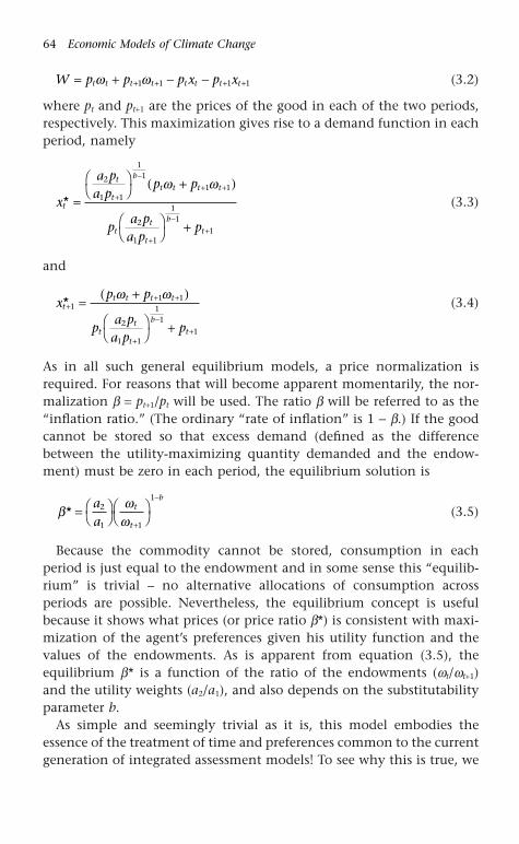
(3.2)

where pt and pt+1 are the prices of the good in each of the two periods,respectively. This maximization gives rise to a demand function in eachperiod, namely

(3.3)

and

(3.4)

As in all such general equilibrium models, a price normalization isrequired. For reasons that will become apparent momentarily, the nor-malization b = pt+1/pt will be used. The ratio b will be referred to as the“inflation ratio.” (The ordinary “rate of inflation” is 1 - b.) If the goodcannot be stored so that excess demand (defined as the differencebetween the utility-maximizing quantity demanded and the endow-ment) must be zero in each period, the equilibrium solution is

(3.5)

Because the commodity cannot be stored, consumption in eachperiod is just equal to the endowment and in some sense this “equilib-rium” is trivial – no alternative allocations of consumption acrossperiods are possible. Nevertheless, the equilibrium concept is usefulbecause it shows what prices (or price ratio b*) is consistent with maxi-mization of the agent’s preferences given his utility function and thevalues of the endowments. As is apparent from equation (3.5), the equilibrium b* is a function of the ratio of the endowments (wt/wt+1)and the utility weights (a2/a1), and also depends on the substitutabilityparameter b.

As simple and seemingly trivial as it is, this model embodies theessence of the treatment of time and preferences common to the currentgeneration of integrated assessment models! To see why this is true, we

bww

* = ÊË

ˆ¯ÊË

ˆ¯+

-aa

t

t

b2

1 1

1

xp p

pa p

a pp

tt t t t

tt

t

b

t

++ +

+

-+

=+( )

ÊË

ˆ¯ +

11 1

2

1 1

11

1

*w w

x

a pa p

p p

pa p

a pp

t

t

t

b

t t t t

tt

t

b

t

* =

ÊË

ˆ¯ +( )

ÊË

ˆ¯ +

+

-+ +

+

-+

2

1 1

11

1 1

2

1 1

11

1

w w

W p p p x p xt t t t t t t t= + - -+ + + +w w1 1 1 1


1403_963363_04_cha03.qxd 6/14/2003 11:18 AM Page 64

need to translate the notation of equation (3.5) into a more familiarform. The endowment ratio (wt/wt+1) corresponds to the growth of the economy, the utility weight ratio embodies the subjective rate oftime preference, and the equilibrium intertemporal price ratio can be straightforwardly transformed into the (endogenous) market rate ofinterest. The substitutability parameter b determines both the intertem-poral elasticity of substitution and the “elasticity of the marginal utilityof consumption.” Once these translations are made, it will be seen thatequation (3.5) is nothing but the formula for the “descriptive” value ofthe discount rate that is typically used in standard integrated assessmentmodels (Cline 1992, Nordhaus 1994, IPCC 1996).

First, in what sense is b just another way of expressing the market rateof interest? Let r be the interest rate as conventionally defined. Thenone unit of the good in the future period is worth 1/(1 + r) units of thegood today. But a unit of the good in the future period is worth pt+1,and a unit of the good today is worth pt. Hence pt+1 = [1/(1 + r)]pt, whichis the same thing as

(3.6)

The change in the endowment from period t to period t + 1 obviouslycorresponds to any economic growth (or decline) occurring over thatinterval, so that

(3.7)

where g is the rate of growth of the economy. Given that the utilityfunction (3.1) is of such a simple time-additive functional form, it isnatural to interpret the utility weight a2 simply as the weight a1 reducedby a factor based on the subjective rate of time preference of the agent.This is consistent with Samuelson’s original (1937) formulation of the DU model (Frederick et al. 2002). If this subjective rate of time preference is given by d, then the relationship is

(3.8)

Returning to equation (3.5) and also using the approximation that (1 + z)g � 1 + gz for small z, we have

(3.9)r b g= + -( )d 1

aa

2

1

11

=+ d

ww

t

t

g+ = +1 1

b = =+

+pp rt

t

1 11


1403_963363_04_cha03.qxd 6/14/2003 11:18 AM Page 65

Finally, for utility function (3.1), easy algebra shows that the intertem-poral elasticity of substitution s is given by 1/(1 - b), and a, the elasticity of the marginal utility of consumption,9 is given by (1 - b).This yields the familiar “descriptive” relationship for the market rate ofinterest

(3.10)

provided the requisite approximations hold.10

Equation (3.10) (or 3.9) already carries within itself the seeds of a cri-tique of current integrated assessment practice. Suppose that the b para-meter lies somewhere between zero (corresponding to a Cobb–Douglasutility function) and -• (corresponding to a Leontief utility function).Then (1 - b) is positive, and the market rate of interest will be greater orless than the rate of subjective time preference, depending on whetherthe economy is showing positive or negative growth. The ordinary prac-tice in integrated assessment is to assume that the economy’s growthwill be positive due to technological progress and capital accumulation.However, it is possible under catastrophic climate scenarios that theamount of the “good” available for consumption could fall. A slowdownin the rate of growth of output brought about by environmental declinewould lead to a lower interest rate than would prevail absent the envi-ronmental damage, and this possibility has been noted by Tol (1994)and Amano (1997). There is no basis for treating current market interest rates as being “descriptive” of future interest rates if the rate ofgrowth of the economy, measured properly to include environment aspart of the material standard of living, is subject to change over time.

In what follows, this theme will be explored in greater depth by speci-fying a second good, “environment,” with a time path of its own thatmay be distinct from the time path of the endowment of the “ordinary”economic good. The next step, however, is to examine the case of morethan one type of consumer. We shall see that this most basic generali-zation of the conventional framework explodes the prescriptions ofexisting climate policy models.

3.3.2 Two agents, one good, two time periods: allowing for intergenerational differences in perspective

To move beyond the “representative agent” in an intertemporal setting,we specify preferences for two distinct agents:

(3.11)u axb

ax

bt

bt

b

1 111

121 1= + +, ,

r g= +d a


1403_963363_04_cha03.qxd 6/14/2003 11:18 AM Page 66

and

(3.12)

The notation here is entirely analogous to that of the single-agent utilityfunction (3.1); the initial subscript on the x variables indicates whichof the two agents’ consumption is being denoted. Both agents have thesame substitutability parameter; this assumption is made purely formathematical convenience. For our purpose here, it is sufficient to dis-tinguish the agents by their utility weights aij and by their endowmentsof the good in the two periods.

Each agent’s maximization of utility subject to the two-period budgetconstraint leads to four individual demand functions, one for eachagent and each dated good. For example, the demand function for agent1 for the good in period t is given by

(3.13)

The endowments are indexed such that wi,j = the ith individual’s endow-ment of the good in period j. The market-clearing equations takeaccount of the fact that there are two agents demanding the good ineach period. Thus, for example, the market-clearing requirement forperiod t is that

(3.14)

The same price normalization, b = pt+1/pt, will be used to find the equilibrium inflation ratio and market rate of interest.

The two-agent model differs significantly from the single-agent modelin two respects. First, the equilibrium interest rate depends on both thecharacteristics of the individual agents’ preferences and on the distri-bution of the good between agents, as well as on the intertemporal distribution of the good. Second, more than one equilibrium is not only possible, but is quite likely given a realistic interpretation of the natureof the differences between the two agents’ preferences.

To demonstrate the first point as simply as possible, consider the case in which the agents’ preferences are Cobb–Douglas, that is, whereb = 0. In that case, the equilibrium inflation ratio b is given by

x xt t t t1 2 1 2 0, , , ,* *+ - - =w w

x

a pa p

p p

pa p

a pp

t

t

t

b

t t t t

tt

t

b

t

1

12

11 1

11

1 1 1 1

12

11 1

11

1

,

, ,

* =

ÊË

ˆ¯ +( )

ÊË

ˆ¯ +

+

-+ +

+

-+

w w

u axb

ax

bt

bt

b

2 212

222 1= + +, ,


1403_963363_04_cha03.qxd 6/14/2003 11:18 AM Page 67

(3.15)

The endowments in period t appear in the numerator of (3.15), whilethose of period t + 1 appear in the denominator. However, unless theutility weights are strictly proportional across agents (so that the utilityfunctions are in effect identical), the inflation ratio (and hence the inter-est rate) will depend on the distribution of the endowments between the twoagents in each period.

This characteristic of the equilibrium, which quite obviously carries over in the case of the more general CES (and other) utility functions,is highly significant for climate policy. The crucial endogenously de-termined interest rate cannot be known without knowing somethingabout both the preferences of the agents and also the distribution of wealth between them in every period. Considerations of “efficiency”cannot be separated from question of “equity.” Because the distributionof the endowment in each period is quite obviously policy-dependent,comparative static assessments of the alternative policies (such as a carbon tax, a permit auction system, or efficiency standards) cannotvalidly be undertaken without specification of the distributional conse-quences of the policies. For, as we have seen in Chapters 1 and 2, the distribution of endowments is quintessentially a policy question,involving as it does the assignment of “rights” of various kinds tomembers of the polity.

Now consider how this two-agent model might be utilized to repre-sent a climate policy simulation in which long periods of time (in particular, periods spanning more than a single generation) might be interpreted. The key question here is whether the extended timeperiod imposes any restrictions on the parameters of the preferencefunctions and the endowments. Suppose we consider time periods longenough to separate the agents into two distinct groups, the “present”and the “future.” The durations of these periods are sufficiently longthat they encompass different generations. In this case, it makes senseto imagine that both the parameters and endowments are “mirrorimages” of each other: The “present” population cares mainly aboutitself, and is endowed mainly with “present” (time t) goods, so that a11 >> a12 and w1,t >> w1,t+1. The opposite holds for the “future” popula-tion; a21 << a22 and w2,t << w2,t+1. As a further simplification, suppose the preferences and endowments are completely symmetrical, so thata11 = a22, a12 = a21, w1,t = w2,t+1, and w1,t+1 = w2,t. With these values, the

bw w

w w* , ,

, ,

=+( ) + +( )

+( ) + +( )+ +

a a a a a aa a a a a a

t t

t t

12 21 22 1 22 11 12 2

11 21 22 1 1 21 11 12 2 1


1403_963363_04_cha03.qxd 6/14/2003 11:18 AM Page 68

equilibrium inflation ratio in the Cobb–Douglas case is 1 and the marketrate of interest is 0.

Preferences and endowments of this type are precisely what onemight expect under the useful fiction of “all transactions taking placeat the initial moment of time.” If we were to imagine all the people who will ever live gathering together in the imaginary marketplace toconduct their transactions at the beginning of time, the preferences andendowments of people who will be alive at different points in time haveto be of this pattern – greater weight placed on consumption occurr-ing when they are alive, and most of their “endowment” occurringduring their own lifetimes. If the pattern is entirely symmetrical withCobb–Douglas utilities, the interest rate is zero, reflecting the equal bargaining power (and similar “fundamental” situation) of the peopleliving at different times.

Why do conventional integrated assessment models fail to reflectthis? It is because all the agents in those models manifest a common“subjective rate of time preference.” Such an assumption may be suit-able for examining the interactions of people who are all alive today,but it is not suitable if we are to imagine people alive at very differenttimes. To see how the conventional models can be misleading, considerwhat happens if both agents exhibit “conventional” preferences, withthe utility weight on period t + 1 consumption equal to a discount factortimes the weight on current consumption. That is, assume in this“present-oriented” case that

(3.16)

with r < 1. In this case, the structure of the two consumers’ utility func-tions is identical. Both have the same subjective rate of time preference.The utility functions differ only by a multiplicative constant (a11/a21)and the agents are identical. This case collapses to that of a single agent,and the inflation ratio is given by (3.5). The conventional “Ramsey rule”holds and the interest rate depends only on the subjective rate of timepreference, the growth rate of the economy, and the substitution parameter.

However, if the agents have different rates of time preference, say r1

and r2, in the Cobb–Douglas case (b = 0) the equilibrium inflation ratiois given by

(3.17)br r w r r w

r w r w=

+( ) + +( )+( ) + +( )+ +

1 2 1 2 1 2

2 1 1 1 2 1

1 11 1

, ,

, ,

t t

t t

a a a a12 11 22 21= =r r


1403_963363_04_cha03.qxd 6/14/2003 11:18 AM Page 69

and once again the interest rate will depend on how the endowmentsare distributed across agents. Suppose agent 2 has a higher rate of timepreference than agent 1 (so that r1 > r2). Then it can be seen from (3.17)that a redistribution from agent 1 to agent 2 in either period willincrease the market rate of interest, and conversely in the case of a re-distribution in favor of agent 1 in either period.

Now, consider more general CES utility functions. Let us focus on thecase in which the utility functions and endowments are symmetrical.The (perhaps) surprising result here is that there will in general be multiple equilibria in this simple model economy. The reason is thatthe mathematical structure of the model is identical to that of the two-consumer, two-good model of Kehoe (1998) that was discussed inChapter 2. The economy can exhibit a positive, negative, or zero marketrate of interest if the intertemporal elasticity of substitution is suffi-ciently low. This makes perfect sense, given the fiction of all agentstransacting at the beginning of time; the equilibrium can favor the“present” individuals with a positive market rate of interest, the “future”individuals with a negative market rate of interest, or be neutral betweenthem (zero rate of interest). Prices and utilities will differ for the indi-viduals in the different equilibria. Yet all three equilibria are Pareto-optimal perfectly competitive equilibria. The multiplicity is a con-sequence of the fact that there is no preferred vantage point in time ifall the agents are imagined to transact simultaneously.

Conventional climate/economy models assume away this possibilityof multiple equilibria by (1) specifying a “representative agent” (oragents with similar time vantage points) and (2) assuming that theintertemporal elasticity of substitution in consumption is relatively high(typically that the utility functions are Cobb–Douglas or logarithmic –see Table 2.4). However, nothing in the logic of general equilibriumrequires these restrictions. Indeed, the more plausible interpretation of the meaning of the utility functions of the individuals who exist atdifferent times is that these utility functions are “symmetric” (or, moreexactly, that each agent’s utility function is “centric” to that agent’s timeperiod) in both utility weights and endowments. This diversity of theutility functions and the time patterns of the endowments, combinedwith a lower degree of intertemporal substitutability than is typicallyassumed, is sufficient to produce multiple equilibria. The properties ofthese equilibria are, as Chapter 2 demonstrated, relatively unexploredin empirical work (because current empirical practice rules them out byassumption). Furthermore, economics offers little or no guidance as to which equilibrium or equilibria the social system will select. As


1403_963363_04_cha03.qxd 6/14/2003 11:18 AM Page 70

Mas-Colell et al. put it, this “is a manifestation of a serious shortcom-ing [in economic analysis] – the lack of a theory of equilibrium selec-tion” (1995, p. 620).11 It may be that current political institutions leadto a “present-centric” equilibrium, but that is not to say that such anequilibrium is an economic choice. Instead, it is a reflection of the waypresent-day political processes are structured to favor one group (thosealive now) over all others (the future generations).

3.3.3 Two agents, two goods, two time periods

Needless to say, all of these results carry over to a situation in whichthere is more than one good as well as more than one type of agent. There are even more permutations of possible outcomes in thiscase. In addition to all the factors discussed in the previous section, themarket rate of interest can depend also on the distribution of endow-ments in the environmental good across the agents, in either period. That is, policies that create or destroy rights to environmental servicesin the future can affect current relative prices of environmental andordinary goods, the market rate of interest, and the current income distribution.

Consider again the minimal case of two agents, two time periods, andnow two goods rather than one. The utility functions of agents 1 and2 will be given by

(3.18)

and

(3.19)

where here xij represents the consumption of the first good (“ordinaryeconomic goods and services”) by agent i in period j, and yij representsthe consumption of the second good “environmental goods and ser-vices” by agent i in period j. Again for simplicity, all of the substitutionparameters are assumed to be equal.12 The endowments of the first goodare denoted by wij, and of the second good by eij.

In this setup, there will be four market-clearing equations (one for theexcess demand for each good in each period) and four prices (one foreach good in each period). Once again, a price normalization is required,so in addition to the familiar inflation ratio there will be two relativeprices,

u axb

ax

bc

yb

cy

bt

bt

bt

bt

b

2 212

222 1

212

222 1= + + ++ +, , , ,

u axb

ax

bc

yb

cy

bt

bt

bt

bt

b

1 111

121 1

111

121 1= + + ++ +, , , ,


1403_963363_04_cha03.qxd 6/14/2003 11:18 AM Page 71

(3.20)

where pj is the price of the first good in period j and qj is the price ofthe second good in period j.

The CES utility versions of this model begin to exceed the capacity ofsymbolic equation solvers such as Mathematica, but the main featuresof the equilibria can be discerned from special cases and numericalexamples. Thus, with Cobb–Douglas utility functions, the (unique)equilibrium for {b, f, y} is given by

(3.21)

(3.22)

f w ee w e

e

= + + +( ) + +( )((((+ +( ) ) ) + + + +( )( )(+ + + +( )(

+ +

+ +

+

1 1 11 21 22 21 22 1 1 21 22 11

11 12 21 2 1 1 11 21 11 22 21 22 1 1

22 11 11 11 12 21 2 1

, ,

, , ,

,

t t

t t t

c a a c c a a c

c c c a c c a c c

a c a c c c tt t

t

t t

t

t

a c c a c c

a c a c c c

a a c c c c

a a c c c

) )+ + + +( )( )((+ + + +( )( ) )+ + +( ) +( )(+ + + +( )

+

+

+

+

we

e we

e

2

12 21 11 21 21 22 1 1

21 11 12 11 12 21 2 1 1

11 12 11 21 11 22 1 1

11 12 11 12 21 2 1

,

,

, ,

,

, )) ) )+( ) +( )((

+ +( ) +( ) +( )+ +( ) +

+

+ + +

+ + + +

+

w we e e e w

e e e e w we e e

2 2 1

11 22 1 2 1 1 2 1 1 1

21 1 2 1 1 2 1 1 1 2 1

22 1 1 1 2

, ,

, , , , ,

, , , , , ,

, , ,

t t

t t t t t

t t t t t t

t t t

a a

a

c cc

a c

a c

t t t t t

t t t t t

t t t t t

21 1 1 1 2 1 1 1 2 1

21 11 2 1 1 2 1 1 1 2 1

1 2 12 1 1 2 1 2 1

e e e w we e e w w

e e e e w

, , , , ,

, , , , ,

, , , , ,

+ + + +

+ + + +

+ + +

+( )) +( )( )+ +( ) +( )(+ +( ) +( ) + 1212 2 1 1 1 2 1e w w, , ,+ + ++( )( )))t t t

y w ee wee w

= + + +( )(((+ + + +( )( ) )+ + + +( )( )(+ +( ( + + ) ) ) ) +

+1 1 12 21 22 21 22 1

11 22 12 21 22 22 2 1

11 22 12 22 21 22 1

22 12 11 11 12 22 2 2

, ,

, ,

,

, ,

t t

t t

t

t t

c a a c c

c c c a a c

a c c a c c

a c a c c c a2121 12 1 2 1

12 21 1 22 1 2 1 2 22 11 1 2 2

11 2 1 2 12 1 2 1 2

c

c c c c a

c a

t t t

t t t t t t t t

t t t t t t

e e we e e w w e e w

e w w e e w w

, , ,

, , , , , , , ,

, , , , , , ,

+( )(+ + +( )( ) +( ) + +( )(+ +( ) + +( ) + tt t

t t t t t

t t t t t t

t t t

a a

c c

a

( ))) )+( ) +( )((

+ +( ) + +( )(+ +( ) +

+

+ +

+ + +

+

we e e e w

e e e e e ee e e e

2 1

12 21 1 2 1 1 2 1 1

22 1 1 1 2 21 1 1 1 2 1

22 1 2 1 1 2 1

,

, , , , ,

, , , , , ,

, , , , ++

+ +

+ + +

( )) +( ))+ +( ) +( )(+ +( ) +( ) + +( )( ))

t t t

t t t t t

t t t t t t t t

a c

a c

w we e e w w

e e e e w e w w

1 2

22 11 2 1 1 2 1 1 2

1 2 11 1 1 2 1 2 12 2 1 1 2

, ,

, , , , ,

, , , , , , , , )

b f y= = =+ +

+

pp

qp

qp

t

t

t

t

t

t

1 1

1


1403_963363_04_cha03.qxd 6/14/2003 11:18 AM Page 72

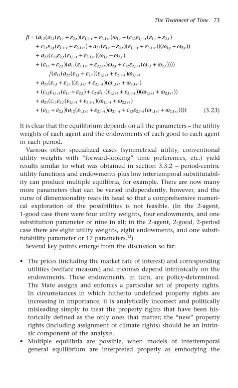
(3.23)

It is clear that the equilibrium depends on all the parameters – the utilityweights of each agent and the endowments of each good to each agentin each period.

Various other specialized cases (symmetrical utility, conventionalutility weights with “forward-looking” time preferences, etc.) yieldresults similar to what was obtained in section 3.3.2 – period-centricutility functions and endowments plus low intertemporal substitutabil-ity can produce multiple equilibria, for example. There are now manymore parameters that can be varied independently, however, and thecurse of dimensionality rears its head so that a comprehensive numeri-cal exploration of the possibilities is not feasible. (In the 2-agent, 1-good case there were four utility weights, four endowments, and onesubstitution parameter or nine in all; in the 2-agent, 2-good, 2-periodcase there are eight utility weights, eight endowments, and one substi-tutability parameter or 17 parameters.13)

Several key points emerge from the discussion so far:

• The prices (including the market rate of interest) and correspondingutilities (welfare measure) and incomes depend intrinsically on theendowments. These endowments, in turn, are policy-determined.The State assigns and enforces a particular set of property rights. In circumstances in which hitherto undefined property rights areincreasing in importance, it is analytically incorrect and politicallymisleading simply to treat the property rights that have been his-torically defined as the only ones that matter; the “new” propertyrights (including assignment of climate rights) should be an intrin-sic component of the analysis.

• Multiple equilibria are possible, when models of intertemporalgeneral equilibrium are interpreted properly as embodying the

b e e e e w e e ee e e e e e e w w

= +( ) +( )(( + +( )(+ +( ) + +( ) +( )) +

+ + +

+ + + +

a a c

c at t t t t t t t

t t t t t t t t

12 21 1 2 1 1 2 1 1 22 1 1 1 2

21 1 1 1 2 1 22 1 2 1 1 2 1 1

, , , , , , , ,

, , , , , , , , 22

22 11 2 1 1 2 1 1 2

1 2 11 1 1 2 1 2 12 2 1 1 2

11 22 1 2 1

,

, , , , ,

, , , , , , , ,

, ,

t

t t t t t

t t t t t t t t

t t

a c

a c

a a

( ))+ +( ) +( )(+ +( ) +( ) + +( )( )))

+( )

+ +

+ + +

e e e w we e e e w e w w

e e e ,, , ,

, , , , , ,

, , , , , , ,

1 2 1 1 1

21 1 2 1 1 2 1 1 1 2 1

22 1 1 1 2 21 1 1 1 2 1 1 1

+ + +

+ + + +

+ + + +

+( )((+ +( ) +( ) +( )+ +( ) + +( )) +

t t t

t t t t t t

t t t t t t t

a

c c

e we e e e w we e e e e e w w22 1

21 11 2 1 1 2 1 1 1 2 1

1 2 12 1 1 2 1 2 1 12 2 1 1 1 2 1

,

, , , , ,

, , , , , , , ,

+

+ + + +

+ + + + + +

( )( )+ +( ) +( )(+ +( ) +( ) + +( )( )))

t

t t t t t

t t t t t t t t

a c

a c

e e e w we e e e w e w w


1403_963363_04_cha03.qxd 6/14/2003 11:18 AM Page 73

preferences of individuals who exist at different points in time. Inparticular, there is no single preferred time vantage point, such as thepresent. Current integrated assessment practice rules out the possi-bility of different intertemporal vantage points by assumption, andthereby produces analytical results that are biased in favor of thepresent population.

• The so-called “descriptive” characterization of the market rate ofinterest is in reality a highly restrictive special case. In particular, itis inconsistent with people living at different times having differentutility functions, and it fails to reveal how the market rate of inter-est depends on distributions of endowments of the various kinds ofgoods in every period.

3.4 Overlapping generations: transactions occur in thepresent, accounting for past history and expectations

3.4.1 A two-period OLG model with one agent in each generation

In keeping with the approach taken in the previous sections, our dis-cussion of OLG models will begin with an examination of the simplestcase. In this model, there is one agent in each generation. The agentslive for two time periods. There is a single good, and each agent isendowed with w0 of the good during the first period of his life and w1

of the good during the second period of his life. The agent born inperiod t consumes xt,t in period t, and xt,t+1 in period t + 1. In this nota-tion, the first subscript denotes the period in which the agent is born,while the second subscript denotes the period in which the consump-tion takes place. The economy can thus be described by Table 3.1,showing the consumption of the good by different agents at differentpoints in time. In this table, total consumption of the good in each timeperiod is given by column sums; thus, consumption in period t is thesum of the consumption by the “young” (those born in t) in period t,which is xt,t, and the consumption of the “old” (those born in t - 1) inperiod t, which is xt-1,t. The boldface entries within Table 3.1 show acomplete account of the consumption values for time periods t - 1through t + 2; the ellipses outside indicate that the table could beextended backward or forward in time by filling in the appropriatespaces.

The utility of an agent is given by a constant elasticity of substitutionutility function depending on the agent’s consumption in each timeperiod, e.g.,


1403_963363_04_cha03.qxd 6/14/2003 11:18 AM Page 74

(3.24)

Utility depends on consumption in the two periods during which theagent is alive, and a1, a2, and b are the parameters of the utility func-tion. For the agent born in t, the price of the good in period t is givenby pt, and the price expected in the next period is pe

t+1. For the agent bornin t - 1, the market price that prevailed in t - 1 is known and the period-t maximization problem of this agent does not depend on expectations.This is the first essential difference between the OLG model and the“simultaneous transactions” model of the previous section. In the OLGframework, the market clears in each period, given past history (that is,the history of past prices pt-1, pt-2, . . .) and the agents’ expectations ofwhat the future periods’ market-clearing prices will be (for those agentswho will be alive in the future period or periods). This modeling twistinvolves a gain and a loss. The gain is that the model is more realisticthan the simultaneous transactions model, because it confines the equi-libration to each successive period and does not require that all periods’markets clear at the beginning of time. The loss is that the equilibriumnow must depend on expected future prices, because the final equilib-rium conditions in the future periods cannot be known in advance by the agents. We shall see that this crucial difference leads to an additional (and irreducible) source of multiplicity in OLG models.

Each agent must make plans based on his lifetime endowment. Thus,the budget constraint for the agent born in t is given by

(3.25)p x p x p pt t t te

t t te

, + £ ++ + +1 1 0 1 1w w

u x xa x

ba x

bt t t t

t tb

t tb

, ,, ,, +

+( ) = +11 2 1


Table 3.1 Time structure of consumption in OLG model

Period born Time period

t - 2 t - 1 t t + 1 t + 2 . . .

t - 3 . . .t - 2 xt-2,t-2 xt-2,t-1

t - 1 xt-1,t-1 xt-1,t

t xt,t xt,t+1

t + 1 xt+1,t+1 xt+1,t+2

t + 2 xt+2,t+2 xt+2,t+3

t + 3 . . .

1403_963363_04_cha03.qxd 6/14/2003 11:18 AM Page 75

where w0 is the endowment of the agent in period t (when he is“young”), and w1 is the endowment of the agent in period t + 1 (whenhe is “old”). For the agent born in t - 1, the budget constraint is

(3.26)

because we are considering the simple case in which the endowmentswhen “young” and “old” are unchanged for each generation.14

Maximization of the utility function (3.24) subject to their budgetconstraints by the two agents who are alive during period t yields theirrespective demands for the good in period t. Finally, we specify that thegood is perishable, so that it cannot be carried over from one period tothe next. Under these circumstances, the market equilibrium in eachperiod is determined by the condition that the sum of agents’ demandsmust equal the total amount of the good available. Thus, market equi-librium in period t requires that

(3.27)

where the starred values are the agents’ demand functions obtainedfrom their budget-constrained utility maximization. Note here that theamount of the good available in period t is the sum of the endowmentsof the good possessed by the “young” agent born in t and the “old”agent born in t - 1.

As usual, a price normalization rule must be chosen, and the naturalone is to normalize in terms of the inflation ratios, b e

t+1 = pet+1/pt and

bt = pt/pt-1. The equilibrium in period t is then defined as the value of bt that solves the market-clearing equation

(3.28)

for some particular expectation-formation mechanism. Before consid-ering the effect of different expectations mechanisms, consider first thecase of the rational expectations steady state. A steady-state equilibrium is one in which the inflation ratio remains constant, and is perfectlyanticipated by the agents. Thus, the steady state embodies a form of“rational expectations,” because the expected values of b coincidein every period with the realized values. Equation (3.28) has two steady-state solutions, given by

w w b

bb

bw w b

bb

w w0 1

2

1

11

2

1 1

11

0 1 1

2

1 1

11

1

0 1 0+

ÊË

ˆ¯ +

+

ÊË

ˆ¯ +( )

ÊË

ˆ¯ +

- - =-

+

-+

+

-+

t

t

b

t

te

b

te

te

b

tea

a

aa

aa

x xt t t t, ,* *+ = +-1 0 1w w

p x p x p pt t t t t t t t- - - - -+ £ +1 1 1 1 1 0 1, , w w


1403_963363_04_cha03.qxd 6/14/2003 11:18 AM Page 76

(3.29)

and

(3.30)

The first point to be noted is that the steady-state equilibrium of this economy is not unique. Unlike in the static case of Chapter 2, this nonuniqueness is not a function of the particular values of the parameters; there are two steady states for any valid parameter set. Thesecond observation is that the steady states have different utility values.In particular, the steady state b1*, usually referred to as the “Golden Rule”steady state, has the higher utility value. It is also clear that the inter-est rate in the b2* steady state depends on the pattern of the endowmentsover time. This feature of OLG models has been noted before (Howarthand Norgaard 1992, Gerlagh and van der Zwaan 2001a, b). This depen-dence of the market rate of interest on the pattern of endowments (orproduction) is intrinsic to intertemporal general equilibrium analysis.

The steady state b2* is referred to as the “autarkic” steady state becauseit has the property that each agent consumes exactly his own endow-ment in each period. Why does the “Golden Rule” steady state havehigher utility? In it, the agents exchange some of their endowments in t so that each can have a higher utility value. This obviously can bebeneficial for the “old” agent (assuming that the endowment is largerduring the “young” segment of life), but what about the “young” agent?If the young agent exchanges some of his endowment with the oldagent, the young agent’s consumption in t is obviously less than itwould have been had he chosen to consume his entire endowment. Heachieves a higher level of utility because in the next period, he will beold and will benefit from the same kind of exchange, consuming morethan his endowment when old. But what guarantee is there that in t + 1 the young agent born in t + 1 will agree to this deal? The youngagent in t can only hope that the same kind of exchange can be arrangedby the agents born in t + 1, t + 2, etc. One kind of institution that mightenable this to occur is some form of Social Security, in which each agentcan treat the utility-increasing exchange as an entitlement. Another way to accomplish the ongoing social contract is through the existenceof fiat money, whose value is “guaranteed” by continuing agreementacross the generations. Both of these mechanisms were discussed inSamuelson’s original (1958) model laying out the OLG framework.

bww2

2

1

0

1

1

* = ÊË

ˆ¯ÊË

ˆ¯

-aa

b

b1 1* =


1403_963363_04_cha03.qxd 6/14/2003 11:18 AM Page 77

Before going on to treat the important question of expectations formation and the path dependence of equilibria in OLG models, let us first examine generalizations of the model to include more than onetype of agent per generation.

3.4.2 Generalizations: OLG models with more than one type ofagent and more than two periods

How do these results change if each generation contains more than one kind of agent? We shall see momentarily that, just as in theArrow–Debreu models, the equilibria will depend on the distribution ofendowments across the different agents. Also, multiple equilibria canarise, depending on whether these agents are both “present-oriented”or not. This distinction will be seen to lead naturally to models in whichthere are more than two periods.

First consider a two-period OLG model with two different agents ineach generation. By now, the utility functions, budget constraints, pricenormalizations, and market-clearing conditions will be familiar. Theutility functions are

(3.31)

(3.32)

These utility functions pertain to the individuals born in t; their utilitydepends on their consumption in the two periods of their lives. Similarutility functions can be written for individuals born in any other period.The equilibrium in period t is again determined by the market-clearingequation specifying that the sum of the demands of all the agents alivein t equals the total amount of the good available. The equilibrium price ratio bt will again depend on the “fundamentals” (preferences andendowments) and on the mechanism by which the agents form expec-tations about the future. The steady-state rational expectations equilib-rium is given by the value or values of b that remain constant over time.

Now it may or may not be surprising that the mathematical form ofthe equation for the steady-state equilibrium in this case is the same asin the Arrow–Debreu case with two agents, one good, and two timeperiods. The utility functions (3.31) and (3.32) have the same form asthose of (3.11) and (3.12); there are four endowments that make up thesupply of the good in period t: those possessed by each of the two youngagents born in t and those possessed by each of the two old agents born

u axb

ax

bt

tb

tb

2 212

222 1

,, ,= + +

u axb

ax

bt

tb

tb

1 111

121 1

,, ,= + +


1403_963363_04_cha03.qxd 6/14/2003 11:18 AM Page 78

in t - 1. The same price normalization can be used, with its same inter-pretation as a transformation of the market rate of interest. The samefindings as in the Arrow–Debreu case carry over: the interest rate willin general depend on the distribution of endowments across agents ineach time period, and multiple equilibria (in addition to the GoldenRule steady state) are possible if the two agents have “symmetrical” pref-erences and the intertemporal elasticity of substitution is not too high.

What does it mean in this case for the utility functions of the twoagents to be “symmetrical”? In the Arrow–Debreu case, the interpreta-tion was that agents living during different time periods would normallyweight most heavily the consumption they enjoy when they are alive,and that their endowments would accrue to them mainly during theirrespective lifetimes. In the OLG framework, we can imagine peoplewhose lifetimes overlap, with each period of the model correspondingto a particular span of the overlapping years. Now it is possible in thissetting to think of two kinds of people: “present-oriented” people whoseutility is grounded in short-term pleasures and whose most importantendowment is in the near term. Imagine a hedonist living “for themoment” whose most important asset is physical attractiveness. Con-trast this with a “future-oriented” person, someone who looks forwardto a high income and high productivity later in life, based on the ac-cumulation of human capital and job experience. These two kinds ofindividuals could be thought of as having the type of symmetrical preferences that lead to multiple equilibria.

It is possible to carry the thought experiment farther, however. Inreality, the periods of overlap of the generations are not sharp and dis-crete as in the model. People are being born and are dying continuously.In any given interval of years, there is a distribution of people of variousages. If we think of the “young” and the “old” people in any such inter-val (corresponding to the two “generations” of the model who are aliveat any time t), we realize that within the “young” there will be peoplewith ages ranging from newborn to middle-aged. Similarly, within the“old” there will be people of ages ranging from middle-aged to octo-genarian (and older). It is plausible for the “young” group then to be madeup of diverse agents with different weights on their consumption (anddifferent endowments) when “young” and when “old.” A middle-agedperson who just happened to fall into the “young” cohort would havea low endowment when young and would place relatively low weighton his consumption when young, compared to his utility weight andendowment when old. Conversely, a very young member of the“young” group would have the opposite kind of utility function (and


1403_963363_04_cha03.qxd 6/14/2003 11:18 AM Page 79

possibly also endowment pattern). The point is that diversity within thegenerations (as captured crudely by the two-agent generalization) is tobe expected.

An alternative way of modeling this type of age-specific diversity is toincrease the number of periods in the individuals’ lifetimes, and to allowfor different kinds of life-cycle endowment patterns. This approachmakes it possible to go back to the single-agent model. It has beenexplored in detail by Kehoe and Levine (1990) in an important paperdealing with the application of OLG models to problems of publicpolicy in general. When the number of periods in the lifetime is three,Kehoe and Levine show that a single-good model calibrated roughly torealistic values for the life-cycle endowments, intertemporal elasticity ofsubstitution, and subjective rate of time discount exhibits the same kindof multiple steady states (with corresponding different interest ratevalues) that we have seen in the two-agent models with symmetricutility functions. Kehoe and Levine specify three 20-year periods in thelifetime of each generation, a subjective rate of time preference of 3.5percent per year, an intertemporal elasticity of substitution of 0.25,15

and a not-implausible endowment pattern of {w0, w1, w2} = {3, 12, 1}.16

This model has three steady states in addition to the Golden Rule (withr = 0). The (annual) market interest rates in these three steady states are 9.1, 1.2, and -17.3 percent. As if this kind of indeterminacy werenot daunting enough, we shall see in the next section that if an OLGeconomy approaches one of its steady states, the one it converges todepends both on the “initial conditions” (the state of expectations atthe outset) and the expectations-formation mechanism of the agents.17

Neither of these considerations is a “fundamental” of the economy.

3.4.3 The indispensable role of expectations

So far, only the steady-state rational expectations equilibria of the OLGmodels have been examined. Of course, restricting equilibria in this wayis quite severe. The actual economy is so complicated that exact knowl-edge of its rational expectations equilibria is impossible in practice(Spear 1989, DeCanio 1999). What happens when the requirement thatthe economy be in its steady-state rational expectations equilibrium isrelaxed? In the OLG model, given the history of the economy up toperiod t, it is possible to calculate the market-clearing equilibrium priceratio in period t given a mechanism for the formation of expectationsabout future prices.

To illustrate what can happen when this is done, the case of a 2-agent,2-good, 2-period OLG model will be considered. We have already seen


1403_963363_04_cha03.qxd 6/14/2003 11:18 AM Page 80

that this model can have multiple steady states if the intertemporal substitutability is low and the agents’ utilities are “symmetric.” Now letexpectation formation take the familiar adaptive form (Nerlove 1958):

(3.33)

Equation (3.33) applies to the intertemporal price ratio variable b; asimilar equation governs the expectations-formation mechanism of therelative price ratio f.

In order to solve for the time path of the price variables, expectationshave to be given initial values b0

e and f0e. Nothing about the fundamen-

tals of the economy determines what these initial expectations valuesmight be. Similarly, it is possible to imagine various values for the speedof adjustment parameter l in equation (3.33) and its counterpart in theequation for ft

e. Numerical simulations show that many different possi-ble starting points and speeds of adjustment are able to produce equi-librium paths that converge to the steady states. This is an illustrationof the general proposition that there is a robust continuum of equilib-ria in OLG models (Geanakoplos 1989b).

This continuum of alternative equilibrium paths will exist even ifthere is only the one steady state other than the Golden Rule. Figure3.1 shows three such paths for b and f for different initial conditionsfor the 2 ¥ 2 ¥ 2 model with Cobb–Douglas utility. Each path convergesto the non-Golden Rule steady state, and different initial conditionswould exhibit different transition paths.18

If there is more than one steady state, the path taken by the economymay converge to a steady state – depending on the starting point andspeed of adjustment – or it may exhibit chaotic dynamics, dependingon how the economic system “picks” the market equilibrium in eachsuccessive period. An example of the kind of behavior that is possibleis given in Figure 3.2, for CES utility functions with a low degree ofintertemporal and inter-good substitutability.19 The economy whosepath is depicted in Figure 3.2 has three steady states, corresponding tob values of 0.115, 1, and 8.686. (The corresponding annual interest rateswould be 11.4, 0, and -10.2 percent if the duration of each time periodis 20 years.) In each time period, the economy uses a numerical searchmethod20 to find the equilibrium, given the past price history and expec-tations formed according to (3.33). With this particular configurationof values, we see that the economy can spend long stretches of time(the 12 periods or 240 years beginning at t = 17 and the 5 periods or100 years ending at t = 37, for example) near its “high interest rate”steady state. From time to time, however, the economy can jump to a

b b l b bte

te

t te

+ = + -( )1


1403_963363_04_cha03.qxd 6/14/2003 11:18 AM Page 81

“low interest rate equilibrium.” At these times the market interest rate is in the vicinity of 1 percent per annum. Note that the “low interest rate equilibria” do not correspond to the future-oriented steadystate (which has a negative interest rate). The interest rate is low butstill positive.


5 10 15 20 25 30 35 40Time

0.4

0.5

0.6

0.7

0.8

Price ratio b

5 10 15 20 25 30 35 40Time

1.05

1.1

1.15

1.2

1.25

1.3

Price ratio f

Figure 3.1 Alternative paths to the steady state: Cobb–Douglas case

1403_963363_04_cha03.qxd 6/14/2003 11:18 AM Page 82

None of this should be taken to suggest that the probabilistic equi-librium choice mechanism underlying Figure 3.2 corresponds to whatactually takes place in the real-world economy. But that is the point: wedo not know by what process the economy seeks equilibrium, or moves fromone equilibrium to another, or cycles between equilibria. If the economyhad spent a long time close to one of its steady states (the “high inter-est rate” one, say) it is not even clear whether the agents could be awareof the existence of other possibilities. It might be that only a shock ofsome magnitude could bump the economy to an alternative equilib-rium. If empirical economics had strong models of dynamics, it mightbe possible to specify how the “equilibrium choice” is made. But thosedynamic models either do not exist or exist in only rudimentary form.But this example and the instability examples of Chapter 2 demonstratethat dynamics matters fundamentally. There is simply no scientific justi-fication for assuming that the economy gravitates quickly to a uniqueand stable equilibrium.

All kinds of variations on these themes are possible. The most obviousdirection in which extension might be made is to the three-period OLGmodel of the type employed by Kehoe and Levine. Given the role ofwealth effects in creating the multiple equilibria, it is also possible toimagine models in which economic growth leads to ever-increasing


10 20 30 40 50Time

0.2

0.4

0.6

0.8

1

Price ratio b

Figure 3.2 Chaotic equilibria: CES utility case

1403_963363_04_cha03.qxd 6/14/2003 11:18 AM Page 83

endowments during the “productive” years. This might trigger a switchfrom a unique equilibrium to a situation of multiple equilibria. How-ever, these possibilities should not distract us from the fundamentalpoints:

• OLG models, like Arrow–Debreu models, can exhibit multiple equi-libria. However, the multiplicities of the OLG models are even morepervasive. Multiple steady states are possible, corresponding to thecase of multiple equilibria in the “full information” models in whichall transactions take place at the beginning of time. In addition, thefact that the OLG models achieve equilibrium period by periodmeans that different initial conditions and expectations adjustmentmechanisms can lead to different transition paths to the steadystates.

• Besides the fact that the equilibria depend on the parameters of theagents’ utility functions and the patterns of their endowments, theequilibrium paths in OLG models also depend on how expectationsare formed and modified. These expectation-formation mechanismsare distinct from the “fundamentals” of the economy. The “rationalexpectations” requirement is far too demanding of information andcomputational capacity to correspond to actual economic processes.

• If the economy does have multiple steady states, the expectations-formation mechanism can lead to chaotic equilibria, in which theprices and interest rate fluctuate according to each period’s selectionfrom among the multiple equilibria available to the agents in thatperiod. This can lead to long stretches of time in the vicinity of dis-tinct interest rates, so that the agents in the economy might not evenbe aware of the potential for an alternative equilibrium based on the“fundamentals” of the economy.

3.5 Models with a social planner or infinitely lived agents

Models in which the agents optimize over an infinite horizon, whetherbased on the interactions of a collection of infinitely lived decision-makers or on the choices made by a social planner having an infinitehorizon, necessarily come up against the problem of how to formulatethe optimization problem into a meaningful mathematical calculation.Maximization of infinite quantities has no meaning. In order to convertthe consumption streams into finite quantities, some kind of constraintor weighting must be used. Thus Ramsey, the first economist to do rig-orous work on this problem, required that there be an upper bound on


1403_963363_04_cha03.qxd 6/14/2003 11:18 AM Page 84

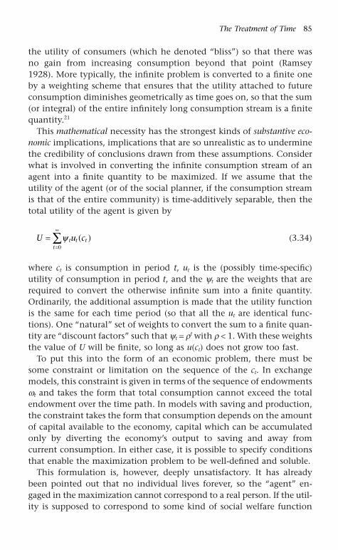
the utility of consumers (which he denoted “bliss”) so that there wasno gain from increasing consumption beyond that point (Ramsey1928). More typically, the infinite problem is converted to a finite oneby a weighting scheme that ensures that the utility attached to futureconsumption diminishes geometrically as time goes on, so that the sum(or integral) of the entire infinitely long consumption stream is a finitequantity.21

This mathematical necessity has the strongest kinds of substantive eco-nomic implications, implications that are so unrealistic as to underminethe credibility of conclusions drawn from these assumptions. Considerwhat is involved in converting the infinite consumption stream of anagent into a finite quantity to be maximized. If we assume that theutility of the agent (or of the social planner, if the consumption streamis that of the entire community) is time-additively separable, then thetotal utility of the agent is given by

(3.34)

where ct is consumption in period t, ut is the (possibly time-specific)utility of consumption in period t, and the yt are the weights that arerequired to convert the otherwise infinite sum into a finite quantity.Ordinarily, the additional assumption is made that the utility functionis the same for each time period (so that all the ut are identical func-tions). One “natural” set of weights to convert the sum to a finite quan-tity are “discount factors” such that yt = rt with r < 1. With these weightsthe value of U will be finite, so long as u(ct) does not grow too fast.

To put this into the form of an economic problem, there must besome constraint or limitation on the sequence of the ct. In exchangemodels, this constraint is given in terms of the sequence of endowmentswt and takes the form that total consumption cannot exceed the totalendowment over the time path. In models with saving and production,the constraint takes the form that consumption depends on the amountof capital available to the economy, capital which can be accumulatedonly by diverting the economy’s output to saving and away fromcurrent consumption. In either case, it is possible to specify conditionsthat enable the maximization problem to be well-defined and soluble.

This formulation is, however, deeply unsatisfactory. It has alreadybeen pointed out that no individual lives forever, so the “agent” en-gaged in the maximization cannot correspond to a real person. If the util-ity is supposed to correspond to some kind of social welfare function

U u ct t tt

= ( )=

•

Ây0


1403_963363_04_cha03.qxd 6/14/2003 11:18 AM Page 85

being maximized by an all-foreseeing benevolent social planner, we run up against the fact that in general it is not possible to construct a social welfare function. The infinite-horizon formulation of theproblem requires specification of cardinal utility on the part of the agentsin order to be able to combine those utilities to obtain a quantity thatcan be maximized. The reason is that the utility in equation (3.34) issummed over the entire (infinite) horizon of the model. In order for thisadding up to be possible, the utilities at different points in time haveto be comparable in the cardinal utility sense. In other words, in orderto treat the succession of individuals living at different times as a singleinfinitely lived agent (or as a single social welfare function that theplanner seeks to maximize), the utilities of the individuals have to bemeasured on a cardinal scale.

This notion of cardinal utility that allows utilities of different in-dividuals to be added together or compared directly originated with the classical utilitarianism of Jeremy Bentham and John Stuart Mill,which sought to ground social ethics in those actions that bring about“the greatest happiness” (Brown 2002). However, such a concept ismeaningless if the utilities of different people cannot be compared quan-titatively. It is just this kind of “interpersonal comparison of utilities”that modern economics eschews. Direct interpersonal comparisons ofutility have been rejected by economists since the 1930s, when it was realized that the theory of demand did not require cardinal utility.22

The invariance of observable demand behavior to monotonic trans-formations of the utility function enables modern welfare economics toadopt a strictly individualist stance.23 The theory has testable implica-tions even though it is not necessary to specify the exact form of theutility function. Certain features of the individual’s preferences, such asthe elasticity of substitution between goods, are intrinsic and invariantunder any monotonic transformation of the utility function, and canin principle be recovered from data on individual behavior. What is notallowed is the aggregation of individual preferences into a single “socialwelfare function” of a particular mathematical form. Hence, welfarecomparisons are permitted only according to the Pareto criterion, thatone situation is better than another if and only if every individual is atleast as well off in the first situation as in the second, and at least oneperson in the first situation is better off. Neoclassical welfare econom-ics is predicated on the notion that individuals are unique and incom-mensurable; they interact through markets according to their ownsubjective interests, but their individual preferences cannot in any


1403_963363_04_cha03.qxd 6/14/2003 11:18 AM Page 86

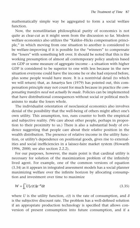
mathematically simple way be aggregated to form a social welfare function.

Now, the nonutilitarian philosophical purity of economics is notquite as clear-cut as it might seem from the discussion so far. Modernwelfare economics also utilizes the “Kaldor–Hicks compensation princi-ple,” in which moving from one situation to another is considered tobe welfare-improving if it is possible for the “winners” to compensatethe “losers” with something left over. It should be noted that this is theworking presumption of almost all contemporary policy analysis basedon GDP or some measure of aggregate income – a situation with higherGDP is considered to be superior to one with less because in the newsituation everyone could have the income he or she had enjoyed before,plus some people would have more. It is a nontrivial detail (to whichwe will return) that, as Amartya Sen (1979) has pointed out, this com-pensation principle may not count for much because in practice the com-pensating transfers need not actually be made. Policies can be implementedthat have distributional consequences without social or political mech-anisms to make the losers whole.

The individualist orientation of neoclassical economics also involvesdenial of the possibility that the well-being of others might affect one’sown utility. This assumption, too, runs counter to both the empiricaland subjective reality. (We care about other people, perhaps in propor-tion to their proximity to us.) There is also a substantial body of evi-dence suggesting that people care about their relative position in thewealth distribution. The presence of relative income in the utility func-tion, or utility’s dependence on positional goods, gives rise to external-ities and social inefficiencies in a laissez-faire market system (Howarth1996, 2000; see also section 2.2.2).

For our purposes, however, the main point is that cardinal utility isnecessary for solution of the maximization problem of the infinitelylived agent. For example, one of the common versions of equation(3.34) as it appears in integrated assessment models has a social plannermaximizing welfare over the infinite horizon by allocating consump-tion and investment over time to maximize

(3.35)

where U is the utility function, c(t) is the rate of consumption, and dis the subjective discount rate. The problem has a well-defined solutionif an appropriate production technology is specified that allows con-version of present consumption into future consumption, and if a

W U c t tt= ( )[ ] -•

Ú e dd0


1403_963363_04_cha03.qxd 6/14/2003 11:18 AM Page 87

boundary condition is met that keeps the value of W finite. The maxi-mization problem becomes one of deciding on the division of outputbetween savings and consumption at each point in time. Solution of the maximization problem under standard conditions yields the“Ramsey Rule” that was derived in the two-period model above (equa-tion (3.10)). However, the solution is not invariant under monotonictransformations of U. Consider

(3.36)

where g is a positive monotonic function. It is easy to imagine g func-tions that would preclude a solution to (3.36) even if (3.35) could besolved. A particularly simple example is g(U) = Uemt, where m > d. ThenW¢ is infinite so long as U[c(t)] is increasing in t. In other words, if aRamsey-type problem such as maximization of W in (3.35) is to besolved, the utility function must be cardinal.24

So far, we have been considering only an economy with a single good,“consumption.” If there are multiple goods and multiple infinitely livedagents, the possibility of multiple solutions to the equilibrium maxi-mization problem arises just as in the single time period case of Chapter2 and in the finite number of periods case of section 3.3.3. Farmer (1999)has shown how this can be demonstrated in an exchange economy pop-ulated by a finite number of infinitely lived agents, with utility func-tions that are additively time-separable. The goods occurring in eachtime period can be thought of as different goods, so that this economyhas a finite number of agents and an infinite number of goods. Negishi(1960) proved that this problem can be converted to one of solving afinite number of equations and unknowns. Furthermore, the reducedproblem has the same mathematical structure as a system of marketexcess demand functions in a finite single-period economy. In general,the system will have multiple solutions.

Thus, even in the simplest type of infinite-horizon model – one withinfinitely lived agents, time-separable utility functions, a discount factor less than one, and bounded wealth of the agents – multiple equilibria can exist. Even strong restrictions on the agents’ utility func-tions and wealth endowments are not sufficient to guarantee unique-ness. The same problems appear as we have seen before, with the sameabsence of definitive empirical information that could point the way to restrictions sufficient to produce a unique solution. The unsatisfac-tory conceptualizations that are required for imagining infinitely livedagents or a benevolent social planner with an infinite horizon do not,

¢ = ( )[ ]{ } -•

ÚW g U c t tte dd0


1403_963363_04_cha03.qxd 6/14/2003 11:18 AM Page 88

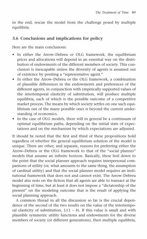
in the end, rescue the model from the challenge posed by multiple equilibria.


Here are the main conclusions:

• In either the Arrow–Debreu or OLG framework, the equilibriumprices and allocations will depend in an essential way on the distri-bution of endowments of the different members of society. This con-clusion is inescapable unless the diversity of agents is assumed outof existence by positing a “representative agent.”

• In either the Arrow–Debreu or the OLG framework, a combinationof plausible differences in the endowments and preferences of thedifferent agents, in conjunction with empirically supported values ofthe intertemporal elasticity of substitution, will produce multipleequilibria, each of which is the possible outcome of a competitivemarket process. The means by which society settles on one such equi-librium out of the many possible ones is beyond the current under-standing of economics.

• In the case of OLG models, there will in general be a continuum ofoptimal equilibrium paths, depending on the initial state of expec-tations and on the mechanism by which expectations are adjusted.

It should be noted that the first and third of these propositions holdregardless of whether the general equilibrium solution of the model isunique. There are other, and separate, reasons for preferring either theArrow–Debreu or the OLG framework to that of the “social planner”models that assume an infinite horizon. Basically, these boil down tothe point that the social planner approach requires interpersonal com-parisons of utility (or, what amounts to the same thing, the assumptionof cardinal utility) and that the social planner model requires an insti-tutional framework that does not and cannot exist. The Arrow–Debreumodel also rests on the fiction that all agents are able to transact at thebeginning of time, but at least it does not impose a “dictatorship of thepresent” on the modeling outcome that is the result of applying thesocial planning approach.

A common thread in all the discussion so far is the crucial depen-dence of the second of the two results on the value of the intertempo-ral elasticity of substitution, 1/(1 - b). If this value is small and withplausible symmetric utility functions and endowments for the diversemembers of society (or different generations), then multiple equilibria,


1403_963363_04_cha03.qxd 6/14/2003 11:18 AM Page 89

with all that they entail for the impossibility of conventional com-parative statics policy analysis, will be the rule. On the other hand, ifthe intertemporal elasticity of substitution is high, then equilibrium islikely to be unique whatever the pattern of utilities and endowments.The allocations, prices, and welfare of the different members of societywill still depend on the policy-driven allocation of endowments (theendowment pattern being taken as a proxy for the various policyoptions available, and for the consequences of climate change), butthere would be a better prospect that conventional integrated assess-ment models would yield reliable insight into the consequences of alter-native policies.

There is a very large empirical literature on the value of the inter-temporal elasticity of substitution (usually denoted by s). As shown here and elsewhere, the value of the “social discount rate” or marketrate of interest, so crucial to the evaluation of climate change damagesand to the costs of mitigation policies, depends on the intertemporalelasticity of substitution25 in a fundamental way. The IPCC’s SecondAssessment Report (1996) contains an explicit discussion of this re-lationship. Yet, amazingly, the IPCC’s review of work on the value ofthis parameter suggests values that are substantially larger than the valuesthat have been estimated by most investigators. According to the IPCC(1996),

Although no consensus has emerged [on the value of the elasticityof the marginal utility of consumption], there is a generally acceptedmethod for approaching the issue. . . .

Individuals in their day-to-day decision making reveal informationabout their perceptions concerning their own utility functions in atleast two different contexts: behaviour towards risk and behaviourtowards intertemporal allocation of consumption. In both contexts,there seems to be a consensus that elasticities of marginal utilities liein the range of 1 to 2, even though the empirical studies requirestrong assumptions about the specific form of the utility function(symmetric and time separable). Thus, one of the most commonlyused utility functions, the logarithmic, implies [an elasticity of themarginal utility of consumption] = 1, meaning that if income risesby 1% the marginal utility of consumption falls by 1%. Attempts byFellner (1967) and Scott (1989) to estimate this elasticity place itsomewhat higher, at 1.5, whereas recent estimates reviewed by Pearceand Ulph (1994) place it in the vicinity of 0.8. (p. 136)


1403_963363_04_cha03.qxd 6/14/2003 11:18 AM Page 90

Given the inverse relationship between the intertemporal elasticity ofsubstitution and the elasticity of the marginal utility of consumption,this implies a range for the intertemporal elasticity of substitution from0.67 to 1.25. (For Cobb–Douglas utility, s = 1.)

Yet macroeconomists (the group of economists who have examinedthe intertemporal elasticity of substitution most extensively) have esti-mated a range of values for s from essentially zero to around 0.3. Forexample, Hall’s (1988) careful econometric analysis of how aggregateconsumption responds to changes in real interest rate expectations is unambiguous: “[A]ll the estimates presented in this paper of theintertemporal elasticity of substitution are small. Most of them are alsoquite precise, supporting the strong conclusion that the elasticity is unlikely to be much above 0.1, and may well be zero” (p. 340).Kocherlakota (1996) shows that it is possible to restate the famous“equity premium puzzle” (Mehra and Prescott 1985) as evidence thatthe coefficient of relative risk aversion26 must be greater than 8.5. Thisis equivalent to saying that the intertemporal elasticity of substitutionis less than 0.12.27 Approaching the problem with an entirely differentmethodology – “survey responses to hypothetical situations constructedusing an economic theorist’s concept of the underlying parameters” –Barsky et al. estimate average lower and upper bounds on the elasticityof intertemporal substitution to be 0.007 and 0.36 respectively, with a midpoint of 0.18 (1997, p. 566).28 As noted above, Auerbach and Kotlikoff (1987) use a value of s = 0.25.

It is a mystery how could the IPCC could have ignored all the evidence and controversy surrounding the empirical value of this keyparameter. The IPCC’s statement itself reflects a high degree of confu-sion – first stating that there is no consensus, then asserting that theconsensus is a value of the elasticity of the marginal utility of con-sumption between 1 and 2. It does not help that the IPCC notes that“for one of the most commonly used” functional forms, the logarith-mic, the crucial elasticity is one; the elasticity of the marginal utility ofconsumption (and of intertemporal substitution) is one by assumptionif logarithmic (or Cobb–Douglas) utility is specified. Of the three empiri-cal studies cited by the IPCC, one was published in 1967 and one is anunpublished mimeo. This can hardly be construed as indicative of aconsensus given the hundreds of articles that have been published inrecent years on individuals’ attitudes towards risk, the equity premiumpuzzle, and related topics, as well as the more recent and statisticallyrigorous estimates of the intertemporal elasticity of substitution itself.


1403_963363_04_cha03.qxd 6/14/2003 11:18 AM Page 91

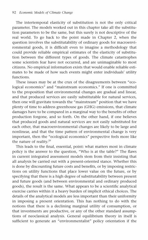
The intertemporal elasticity of substitution is not the only criticalparameter. The models worked out in this chapter take all the substitu-tion parameters to be the same, but this surely is not descriptive of thereal world. To go back to the point made in Chapter 2, when the question involves the substitutability of ordinary goods for macroenvi-ronmental goods, it is difficult even to imagine a methodology thatcould provide reliable empirical estimates of the elasticity of substitu-tion between the different types of goods. The climate catastrophessome scientists fear have not occurred, and are unimaginable to mostcitizens. No empirical information exists that would enable reliable esti-mates to be made of how such events might enter individuals’ utilityfunctions.

These issues may be at the crux of the disagreements between “eco-logical economics” and “mainstream economics.” If one is committedto the proposition that environmental changes are gradual and linear,and that produced services are easily substitutable for natural services,then one will gravitate towards the “mainstream” position that we haveplenty of time to address greenhouse gas (GHG) emissions, that climatedamages have to be compared in a marginal way to the benefits of otherproduction forgone, and so forth. On the other hand, if one believesthat produced goods and natural services are not easily substituted foreach other, that macroenvironmental changes are likely to be large andnonlinear, and that the time pattern of environmental change is veryimportant, then the “ecological economics” perspective feels more likethe nature of reality.29

This leads to the final, essential, point: what matters most in climatepolicy is the answer to the question, “Who is at the table?” The flawsin current integrated assessment models stem from their insisting thatall analysis be carried out with a present-oriented stance. Whether thisis done by discounting future costs and benefits, or by imposing restric-tions on utility functions that place lower value on the future, or byspecifying that there is a high degree of substitutability between presentand future goods (and between environmental and ordinary producedgoods), the result is the same. What appears to be a scientific analyticalexercise carries within it a heavy burden of implicit ethical choices. Thedetails of the analytical models are less important than their uniformityin imposing a present orientation. This has nothing to do with thenotions that there is a declining marginal utility of consumption, orthat investments are productive, or any of the other standard assump-tions of neoclassical analysis. General equilibrium theory in itself is sufficient to generate an “environmentalist” policy orientation if the


1403_963363_04_cha03.qxd 6/14/2003 11:18 AM Page 92

models are set up in such a way as to make sure that all agents arepresent and represented in the market.

Of course, in practical terms the representation of people not yet borncan only take place through applications of principles. How to do thisshould be a major item on the research agenda for climate policy analy-sis, and for the political discussion of climate issues. General equilib-rium theory as we currently know it can provide some guidelines, bothpositive and negative. We can see what equilibria look like when peoplefrom different time periods engage in model transactions, and we candiscern the consequences of imposing a present-oriented slant on modeldesign. It is clear from the examples discussed in this chapter that economic logic shows no preference for individuals of different timeperiods; the present-centric bias that comes with ordinary discountingis an artifact of incomplete models or hidden assumptions. It is difficultto translate the outcomes of hypothetical general equilibrium modelsinto working principles for policy design. Even so, development of theseprinciples should be a focus of research and political discussion. Realprogress in the climate debate has first to resolve the question of whoseinterests are being represented, through a transparent and completespecification of how various kinds of rights are to be assigned. Then thepower and elegance of general equilibrium analysis can be brought tobear to explicate the nature of the choices we face. Current practice onlyhides the essential questions behind a technical facade.


1403_963363_04_cha03.qxd 6/14/2003 11:18 AM Page 93

4The Representation of Production

94

4.1 Introduction

“Tastes” and “technology” are the fundamentals upon which neoclassi-cal general equilibrium models are built. While the representation oftastes is expressed through utility and demand functions, the underly-ing productive technology of the economy is represented by productionfunctions that relate various quantities of various inputs to the outputproduced by firms. This approach requires a behavioral theory thatdescribes the activity of firms as they carry out the processes of produc-tion. The behavioral theory is profit maximization, which parallels theutility maximization of consumers on the demand side of the economy.While some of the conceptual and mathematical difficulties that plaguethe representation of preferences are common to the treatment of pro-duction in the models, there are several important differences.

Because of the way firms are defined, there are no wealth effects thatcould create the kind of multiple equilibria that we have seen inexchange models that embody consumer preferences.1 Consumers maxi-mize utility subject to their budget constraints, which, as in the modelsof Chapters 2 and 3, depend on the endowments of the different kindsof goods over which the consumers have property rights. In the neo-classical representation of the firm, the firm has no endowments – itsimply hires factors of production and maximizes profits, subject to itstechnology of production. Because it has no endowments of inputs,there can be no wealth effects associated with changes in relative inputprices. As a consequence, the factor demand curves are invariably downward-sloping functions of the factor’s “own price.”

Mathematically, imagine a firm that produces a single output with a market price p. (There is no difficulty in generalizing to multiple

1403_963363_05_cha04.qxd 6/14/2003 11:20 AM Page 94

outputs.) The conventional assumption (as in Chapters 2 and 3) ofperfect competition will be maintained throughout. Then, if the factorsof production are x1, x2, . . . , xm with prices w1, w2, . . . , wm, and the pro-duction function transforming the inputs into output is f, the firm maximizes profit

(4.1)

The first-order conditions for a maximum (with x1*, x2*, . . . , xm* being theequilibrium values) are

(4.2)

There are no endowments in equation (4.2), hence the absence of any of the wealth effects. Indeed, it is easy to show that, provided thesecond-order conditions guaranteeing a maximum hold, the “ownprice” factor demand curves are downward sloping (Silberberg 1990),that is

(4.3)

Similarly, it is very easy to show that equilibrium profits cannot increaseif the price of any factor of production increases. Thus, if p* is themaximum profit for a particular set of factor prices,

(4.4)

then for any particular input j,

(4.5)

because each of the terms in the bracketed summation in (4.5) is zerofrom the first-order conditions. An argument such as that embodied inequation (4.5) is the reason for many economists’ skepticism about the“Porter hypothesis” – the notion that stricter environmental regulationcan, under some circumstances, have a beneficial effect on corporate

∂∂

∂∂

∂∂

∂∂

p* *, *, . . . , ** *

*

*, *, . . . , **

*

*

wp f x x x

xw

wxw

x

pf x x x wxw

x

x

ji m

i

ji

m

ii

ji

m

j

i m ii

i

jj

j

= ( ) - -

= ( ) -[ ] -

= - <

= =Â Â

Â

1 21 1

1 2

0

p * *, *, . . . , * *= ( ) -=Âpf x x x w xm i ii

m

1 21

∂∂xw

ii

i

*< "0

pf x x x w ii m i1 2*, *, . . . , *( ) = "

p = ( ) -=Âpf x x x w xm i ii

m

1 21

, , . . . ,

The Representation of Production 95

1403_963363_05_cha04.qxd 6/14/2003 11:20 AM Page 95

performance and profitability. Tighter environmental regulation is, inthe conventional view, equivalent to an increase in the price of one ofthe “inputs” to production, where the input is considered to be a pol-lutant and the price is the cost that is imposed, implicitly or explicitly,by the environmental regulation. If the firm is optimized and the com-bination of the behavior and technology or production is described inthe framework of equations (4.1)–(4.4), then the increase in environ-mental stringency cannot increase profitability.2

Once the “problem of production” is stated in this manner, however,several difficulties are apparent. First, some firms actually do possessendowments of goods. Oil companies are one example. This is not reallya valid objection to the framework of equations (4.1)–(4.4) because itcould be argued that the companies had to pay for their rights to theoil, or, more fundamentally, that the actual owners of the resource arethe shareholders of the company, and that the task of the managementof the company is simply to maximize profits given the firm’s technol-ogy. “Rents” would have to be paid to the owners of the oil no matterwho they were, or conversely, the owners of the oil would sell it at its market price regardless of whether “their” firm or some other werethe buyer.

A more serious objection arises in the treatment of technologicalknowledge as something that can be adequately represented by a pro-duction function transforming commodity inputs into output. Whilesuch a representation might be sensible under unchanging pastoral conditions, it is far less clear that it is appropriate in the modern worldcharacterized by rapid technological change. Furthermore, what of thebehavioral model? We know that the managers of firms do not spendtheir time solving the maximization problem (4.1); they are insteadengaged in a multitude of activities of varying levels of difficulty, requir-ing an entire range of human capabilities from leadership to the appli-cation of the insights of mathematical finance. At the most fundamentallevel, the production function and profit maximization representationof the firm gives no insight into why firms exist at all. How are theboundaries of firms determined? Why do actual business organizationscarry out some activities themselves, while contracting out other func-tions and purchasing yet others in the market?3

The mathematics of (4.1)–(4.4) is simple and its implications arestraightforward. What, then, of the myriad of evidence that firmsdisplay inefficiencies and experience difficulties of all sorts? Why arefirms so diverse, to the point that some prosper and others fail? Whyare top managers so highly compensated? We shall see that deep defi-


1403_963363_05_cha04.qxd 6/14/2003 11:20 AM Page 96

ciencies in the production function/profit maximization model arisefrom a number of sources. Yet despite these red flags, the practice in the economic models used for climate policy analysis is universally torepresent production in some (often quite elaborate) version of the pro-duction function/profit maximization model.4 The consequences of thispractice are very strong, and the result is an upward bias in estimatesof the costliness of climate protection measures. As in the case of con-sumer preferences, the subtleties of the behavior of firms as they operatein the real world are well-known both within and outside the econom-ics profession. What is missing is a realistic application of those insightsto the construction of climate policy models.

4.2 The modern theory of the firm

Suppose we begin by accepting, in the spirit of the “inside critique” ofChapter 2, that firms and other productive organizations are collectionsof rational, self-interested individuals. At the foundation of the pro-duction function/profit maximization story is the notion that the firmis efficient. That is, profits are maximized given the technological pos-sibilities embodied in the production function. The consequence of thismaximization is a series of first-order conditions equating factor pricesto marginal products. These equalities in turn form the starting pointfor econometric estimation of production and supply functions and of comparative statics calculations of how the firm would respond tochanges in market conditions. (The “proof” in equations (4.4)–(4.5) thatprofits cannot increase if environmental regulations are tightened is anexample of such a comparative statics exercise.)

The most basic insight of the modern theory of the firm is that theindividual rationality of the members of the firm does not guarantee,and in fact is likely to be a barrier to, the “rationality” of the organiza-tion, defined as optimal profit maximization. The interests of the indi-viduals making up an organization are not identical to the interest ofthe organization as a whole. There are substantial areas of overlap ininterests, of course – in the extreme, if a firm goes out of business itsmembers are unemployed5 – but the task of aligning the actions of themembers of the organization with the organization’s formal goal is aformidable one.

This is a leading example of the well-known problem of collectiveaction. The wide scope of this problem was set out with great clarity byOlson (1965), but awareness of it has been with us since the earliesttimes. The precise nature of the divergence between the interests of the


1403_963363_05_cha04.qxd 6/14/2003 11:20 AM Page 97

individuals making up a group and the interest of the group as a wholehas been described in various ways, as the principal/agent problem, theproblem of opportunism, and the problem of information asymmetry.All these descriptions are ways of looking at similar sets of difficulties,so it is worthwhile to discuss some of the specifics of the argument.There is an extensive technical literature spanning economics, man-agement science, sociology, and organization theory that covers theseissues in detail, and no attempt will be made here to survey that liter-ature comprehensively.6 Instead, the main arguments will be reviewedin somewhat generic form. What is common to all these literatures is aconsensus that the simplistic production function/profit maximizationframework does not and cannot serve as an adequate description of theactivities of firms and other productive organizations in a moderneconomy.

4.2.1 Principal–agent problems

All human relationships have at least the potential for a divergence ofthe interests of the parties. While cooperation is necessary for any kindof complex production or market interaction, it should not come as asurprise that the leaders (or owners) of firms must struggle with how toinduce the members of the firm to advance the firm’s objective – whichis, at the most basic level, to increase the owners’ wealth. The conflictsthat can come into play in relationships of this type (which are not con-fined solely to the modern business corporation) are referred to as “prin-cipal–agent problems” because the interests of the “principal” (who maybe the shareholders of a firm, the top management, or some subgroupof the organization) and the “agent” (the employees of the firm, a management layer below the top, or a subordinate subgroup) do notcoincide.

Some principal–agent problems arise simply because of conflicts ofinterest. Owners of a firm may wish that their employees would putprofit maximization above all other goals, but it is impossible to specifyin detail every eventuality in which management discretion is required.That is, after all, one reason for hiring managers in the first place. Inthe natural course of events, situations are bound to arise in which themanagers’ interests and those of the owners differ. The consequences of this “separation of ownership and control” were remarked upon byBerle and Means in the 1930s, but recognition of the problem goes back to Adam Smith and before (Berle and Means 1932; Jensen andMeckling 1976).7


1403_963363_05_cha04.qxd 6/14/2003 11:20 AM Page 98

Managers are very likely to be privy to information that is unavail-able to the owners of a firm. Under such circumstances, the owners have no way of assessing whether the managers’ decisions are based oninformation only the managers have, or are being driven by some dis-tinct interest of the managers. Is the construction of opulent corporateoffices necessary to maintain the company’s image and to provide a kindof advertising (or signaling), or does it merely flatter the vanity of management? Is entering a new line of business justified on strategicgrounds of profit potential, or is it the managers’ empire building? Is acorporate jet necessary to economize on scarce managerial resources, or is it a perquisite that could be dispensed with to the benefit of thebottom line? The very disconnection between the advancement ofcapital on the one hand, and immersion in the day-to-day operationsof the firm on the other, that makes modern market capitalism possible is also the source of this kind of information gap. The inability of the principals to know the actual rate of return on variousinvestment projects may induce them to set a “hurdle rate” higher than the appropriate risk-adjusted cost of capital, as a way of assuringthat profits are not dissipated into managerial slack (Antle and Eppen1985). This means that some genuinely profitable projects will not be undertaken, and that the firm’s production process will be inefficient asa result.

Principal–agent problems also show up in the design of compensa-tion plans for managers and employees. Stock option plans, investmentof employees’ retirement savings in company stock, and bonuses basedon company or division-wide profit performance are all examples of theattempt to conjoin the interests of the agents of a company with thoseof their principals. These plans can themselves have adverse repercus-sions for efficiency, as when managers concentrating on short-runresults (because that is what determines their compensation) emphasizetemporary gains over long-term opportunities (Statman and Sepe 1984;Pinches 1982), or when the compensation plans are nothing butschemes to conceal managers’ collection of excessive rents (Bobchuk et al. 2001).

4.2.2 Problems of control

Even if a divergence of interests between owners and managers (orbetween different levels of managers, or between management andworkers) did not exist, a modern complex organization would face dif-ficulties of control. What are the instructions to be given to lower


1403_963363_05_cha04.qxd 6/14/2003 11:20 AM Page 99

management and employees in directing them to maximize profits? Themodern firm is not like a Robinson Crusoe sole proprietorship or smallfamily workshop; no one working on the assembly line, on the roadmaking sales, or sitting in a customer service cubicle, can possibly knowabout all aspects of the firm’s multitudinous activities. Even the topmanagement cannot know everything; information is filtered as it risesthrough the bureaucracy. It surely will not do simply to instruct employ-ees to “maximize profits,” because no one can know exactly what any person’s or group’s contribution to the final economic profit of the firm is. Employees have to be given particular tasks and respon-sibilities; they have to be provided with information systems that enablethem to track their progress (and that enable their performance to beevaluated), and specialization within the organization is important in the same way and for the same reasons it is at the industry oreconomy-wide level.

As a result, the command to “maximize profits” must be mediated bylayers of accounting data, direct and indirect performance indicators,internal and external benchmarks, and judgment of intangibles. Every-one knows the pitfalls of having agents work “to the formula” that hasbeen provided as their performance guideline, regardless of the long-term objective. The net profitability of a firm is the result of a complexof decisions made at different levels of the organization, influenced byan external environment (customers, laws and regulations, market con-ditions) that can only be known imperfectly. Employees have to bemotivated to align their actions with the formal objectives of the firm,and the organization must interact with the larger society – its com-munity or communities, the legal system, and “public opinion.”

All of these considerations are only a part of what makes manage-ment such a demanding task. If maximization of profits along the linesof equation (4.1) were all that was involved, the ideal manager wouldbe a recent college graduate who had done well in beginning calculuscourses. There would be no multimillion dollar salaries for top man-agers, nor would there be a scramble by students for admission to high-priced MBA programs.

4.2.3 Deeper computational limits

At the most fundamental level, the fact that the firm can only makedecisions through its own rules and procedures imposes certain limitson its ability to process information. No matter how capable the indi-viduals making up the firm are (and psychological research, experi-mental evidence, and introspection suggest strongly that individuals


1403_963363_05_cha04.qxd 6/14/2003 11:20 AM Page 100

themselves are only boundedly rational), the organization does nothave a unitary consciousness and does not act in the same way as anentity with a single will. While some advantages can be gained bydrawing on the distributed information and intelligence of the indi-viduals who make up the organization, the decision-making proceduresof the organization impose one or more layers of complexity on theformation of decisions. Whether these procedures are thought of as amechanism for aggregating the preferences of the individuals in the firm(as might be appropriate for an owner-operated firm or a relatively smallpartnership) or whether the rules emerge from legal, cultural, and historical structures, there can be no assurance that the resulting decisions will accomplish any particular singular objective such as profit maximization.8

The nonunitary nature of the firm imposes computational constraintson the firm’s decision-making that preclude complete maximization.Many of the actual problems firms face, such as sequencing and sched-uling, database management, storage and retrieval, or network design,can be formalized in such a way that they can be shown to belong tothe class of NP-complete problems (Garey and Johnson 1979). Mathe-matically, this means that there is no known algorithm for solving anyof these problems that does not require an amount of computation timethat grows faster than “polynomially” in the size of the problem.9 Infor-mally, it means that these problems are intractably difficult and that inpractical applications, such as the operation of a productive organiza-tion, the managers will have to settle for approximations that fall shortof an optimal solution. It is also known that a number of standard prob-lems in economics, including the formation of “rational expectations”and the solution of standard problems in game theory and general equi-librium, run up against computational limits (see Rust 1996 [revised1997], DeCanio 1999, and the references cited in these papers). Even ifhuman brains are somehow able to access quantum computationaleffects, communication over “classical” channels, as required in humanorganizations, means that problems requiring combining informationfrom the various members of the organization are subject to the limitsof a classical Turing machine.

The strong implication is that there is no way around the limits that“bounded rationality” places on human economic activity.10 In par-ticular, it is impossible to achieve the mathematical ideal of full opti-mization in production processes and the other activities of firms.Simply recasting these problems as calculus maximization exercises that can be solved amounts to abstracting from essential features of the


1403_963363_05_cha04.qxd 6/14/2003 11:20 AM Page 101

underlying reality. The fact that it is usually possible to calculate theoptimal solution of equation (4.1) is not sufficient grounds for assert-ing implicitly that (4.1) is in fact an adequate representation of the technological and behavioral reality of the firm.

4.2.4 The evidence

The issues discussed so far in sections 4.2.1–4.2.3 constitute a com-pelling set of theoretical reasons why we should not expect optimiza-tion to be the rule for firms and other productive organizations. Inaddition to these abstract arguments, there is a very large body of evi-dence that is consistent with a failure of complete optimization in pro-duction. The first and most obvious type of evidence is the personalexperience we all have had in our own organizations – each of us knowsof a myriad of inefficiencies close to home. It is not necessary to relyonly on subjective experience to establish that inefficiency in produc-tion is the rule rather than the exception, however. Several currents inthe empirical literature of economics, management science, and opera-tions research are devoted to the measurement of inefficiencies in pro-duction. In a series of papers beginning in 1966, Harvey Leibensteinintroduced the concept of “X-efficiency” (and also its converse, X-inefficiency) and argued that X-efficiency was more important thanallocative efficiency in determining the productivity and profitability offirms.11 Although Leibenstein is most often acknowledged for his theo-retical contribution, it should be remembered that his original 1966paper contained a great deal of empirical information on the existenceand magnitude of X-inefficiency, including data from detailed surveysof industrial establishments, the lag time between invention and inno-vation (or the adoption of the new technology), and the rate of returnto management consulting services.

One way of formalizing the notion of technical efficiency (and ofmeasuring the distance a firm or facility is from its production-possibilities frontier) is through the technique of “data envelopmentanalysis” (DEA). Originally introduced in the 1950s (Koopmans 1951,Farrell 1957), the DEA technique calculates the efficient points on theisoquant or production-possibilities frontier for a group of individualdecision-making units (DMUs). The DMUs that lie on the frontier are“technically efficient,” while those that lie inside it are inefficient. Ineffect, DEA is a flexible method for “benchmarking” DMUs to the mostefficient comparable units in their industry.

Several comprehensive standard treatments of DEA are available(Cooper et al. 2000, Charnes et al. 1994, Sengupta 1995). The DEA


1403_963363_05_cha04.qxd 6/14/2003 11:20 AM Page 102

literature itself is extensive; the CD-ROM bibliography (Seiford 2000)accompanying the Cooper et al. text and covering the period 1978through September 1999 contains over 1500 entries.12 Articles contain-ing “data envelopment analysis” in their title, keywords, or abstracthave been running at a rate of around 100 per year in recent years inthe Social Sciences Citation Index (ISI Web of Science 2002). It wouldbe an interesting (although extremely time-consuming) exercise toconduct a complete meta-analysis of this literature to determine if thereare any patterns or tendencies in the levels of inefficiency reported; a nonsystematic compilation of 26 such studies revealed an average efficiency level of 86 percent (DeCanio 1997).

DEA is not the only approach to the measurement of relative effi-ciency. DEA is a nonparametric technique, but parametric methods havealso been applied to the problem.13 In addition, there are other indica-tions of the failure of profit maximization to account for what weobserve in the real world. If firms were fully optimized, there would be no market for corporate control, and no efforts by management toinsulate themselves from takeovers by defensive measures such as supermajority provisions and “poison pills.” Successful takeover at-tempts tend to raise the value of the stock of both the target and ac-quiring firms (Jensen 1988, Bradley et al. 1988, Jarrell et al. 1988), andthere is evidence that when states pass antitakeover legislation, thevalue of firms headquartered in those states falls.14 All these evidencesof the failure of firms to optimize are observationally grounded. It canhardly be considered good scientific practice to ignore such extensiveand diverse evidence of the failure of optimization in favor of an unsub-stantiated preference for the unadorned profit maximization model offirms and production.

4.3 Aggregation problems

In addition to the deficiencies in profit maximization as a behavioralhypothesis, there are also technical obstacles to the representation ofproduction by conventional neoclassical production functions. If tech-nological production possibilities are to be represented by any meansother than an exhaustive listing of every individual piece of equipmentalong with directions for its use, the production function must embodysome notion of capital aggregation. Yet no economically meaningfulmethod of constructing capital aggregates can be devised, except underconditions that are so unusual and special as to have no relevance tothe real world.


1403_963363_05_cha04.qxd 6/14/2003 11:20 AM Page 103

The basic problem is that the price of capital goods depends on theexpected future stream of profits that can be earned through theiremployment. This future net revenue stream has to be discounted by adiscount rate that itself is the price of capital, but such a self-referentialpricing problem would not in and of itself preclude a solution (equa-tions involving their own solution as a functional argument can oftenbe solved for their “fixed points”). The real problem is the uncertaintythat is intrinsic to technological progress. For it is always possible that new inventions will render elements of the existing capital stockobsolete and worthless. (Recall the example of the electromechanicalcalculators from Chapter 2.) No measurement of “capital” based on pastdollars invested can escape this possibility, and hence the value of thecapital stock is always contingent upon the unknowable future state oftechnology.

This conundrum has been elaborated in a number of different ways.Joan Robinson (1953) made clear that the attempt to reconcile the deci-sion-making of the “man of deeds” (the capitalist business ownermaking investment decisions based on expected future profits) and the“man of words” (the economist or accountant attempting to measurethe capital stock as something other than an exhaustive list of differenttypes of equipment) was impossible under any but the most rigid kindof unchanging conditions. A more recent argument with similar impli-cations is given by Fisher and McGowan (1983; see also Fisher et al.1983), who demonstrated that the true (“economic”) rate of returncannot be recovered from accounting data.15 As Fisher puts it, “[w]hilethe economic rate of return is the magnitude that properly relates astream of profits to the investments that produce it, the accounting rateof return does not. By relating current profits to current capitalization,the accounting rate of return fatally scrambles up the timing” (1984,pp. 509–10).

The capital aggregation problem is not just one of measurement. Ina series of articles published in the Review of Economic Studies (1965,1968a, b) and Econometrica (1969a) and summarized in his definitiveEconometrica paper (1969b), Fisher describes (and solves, to the extentthat it can be solved) the problem of defining aggregate capital stocksand constructing aggregate production functions. In brief, the mainresults are:

(1) Unless efficient allocation of resources is assumed,16 an aggregateproduction function will exist if and only if every firm’s productionfunction is additively separable in capital and labor;


1403_963363_05_cha04.qxd 6/14/2003 11:20 AM Page 104

(2) If an efficient allocation is assumed, and if labor exhibits strictlydiminishing returns, then a necessary and sufficient condition forcapital aggregation (and existence of an aggregate production function)is that every firm’s production function satisfy a partial differentialequation of the form

(4.6)

where the function g is the same for all firms. Here the f v are the pro-duction functions of the individual firms (indexed by v), and the sub-scripts indicate marginal products or cross-products with respect to thefirms’ capital and labor inputs. This condition is not easy to interpretdirectly, but it has two consequences:

(2a) If constant returns is not assumed, “there is no reason why per-fectly well behaved production functions cannot fail to satisfy anypartial differential equation [of this] form,” and “if some firm has sucha production function, then exact capital aggregation is impossibleregardless of the nature of the production functions of other firms”; and

(2b) If constant returns is assumed, then “average product per worker(as well as marginal product) and profits per worker will be the same inall firms” (1969b, pp. 559–60, italics in the original).

Of course, it would be stretching reality past the breaking point topresume that average product per worker and profits per worker are thesame in all firms, whether in the whole economy or in any subsectoror industry within the economy. If this were not bad enough, the technical conditions for the construction of subaggregates (that is,aggregates comprised of some but not all types of capital) are also veryrestrictive. Nor is it the case that an aggregate production function with nice properties can be found that closely approximates the truedisaggregated production function. The only way in which such ap-proximations could be assured would be if we were willing to acceptproduction functions that are very “irregular” in the sense that theirfirst and second derivatives exhibit large “wiggles” up and down. Fisheris not entirely pessimistic about the possible usefulness of aggregate pro-duction functions, but he concludes on this note:

Just because it is possible to use aggregate production functions forgrand statements about long run growth and technical change, it isimportant to be careful about the foundation for such statements. At

ff f

g f vKLv

Kv

LLv L

v= ( ) "


1403_963363_05_cha04.qxd 6/14/2003 11:20 AM Page 105

present, that foundation seems solid only insofar as relatively smallchanges are concerned. The analyses which I have here summarizedhave convinced me that there is at least need for great caution inthis area. It may recalled that Solow’s seminal article [1957, p. 312]called for “more than the usual ‘willing suspension of disbelief’ totalk seriously of the aggregate production function.” That suspensionhas clearly led to very fruitful results. I am, however, finding it in-creasingly difficult to maintain. The conditions for the existence ofaggregate production functions, at least when widely diverse indus-tries are included, seem very, very strong. (1969b, p. 576)

What are the implications of these findings for current practice inintegrated assessment modeling? The models are not based on anyexplicit tests of whether the conditions required for aggregation of production functions hold.17 This means that even if the productionfunctions of the models bear some kind of statistical relationship to past data, the production functions cannot therefore be taken to beempirically grounded. Instead, they represent a fiction that is mathe-matically convenient, one that enables the derivation of optimality con-ditions (expressed as the first-order conditions for profit maximization)that might be useful for policy analysis if they actually did obtain. Theplausibility of this fiction may vary according to the perceptions of the consumers of the models’ results, but that kind of postmodern attitude (that “reality” is in the eye of the beholder) is at variance with the cloak of scientific rigor in which the models are typicallywrapped.

4.4 A more realistic characterization of production

We have seen in Chapter 2 that the mathematical behavior of a tâton-nement adjustment process depends on the characteristics of the marketexcess demand functions. Without knowledge of the actual dynamicsof the economic system, comparative statics analyses of the response ofthe system to policy changes are not reliable. The excess demand func-tions derived from standard utility-maximizing assumptions can havevirtually any shape, so that the use of equilibrium conditions to char-acterize the economy leads to an underdetermined system. This suggeststhat the dynamic processes themselves might be a better starting pointfor modeling than the conditions of equilibrium. A true dynamic modelcould trace out the development of the system over time, whether ornot it tends towards equilibrium (and regardless of the characteristics


1403_963363_05_cha04.qxd 6/14/2003 11:20 AM Page 106

of any equilibrium that might exist). If the dynamics were known, noinformation about the behavior of the system would be lost or missing,whereas we have seen that knowledge of the equilibrium conditionsalone is not sufficient to determine the system’s characteristics. A focuson dynamics rather than equilibrium may also be a better way toapproach the representation of production.

There is no doubt that the problem of dynamics is difficult, and hasnot been satisfactorily solved (at least there is no consensus about whatconstitutes a good dynamic economic model). One way of addressingproduction dynamics that has much to recommend it is an evolutionaryperspective. Evolutionary models have the advantage of being well-suited to complex systems, and the pressure of “natural selection” ishighly analogous to the market pressures faced by firms in a competi-tive environment. Evolutionary thinking about economic dynamics hasa long and distinguished history. Hayek (1988) argued that the idea ofevolutionary change in the social sciences and humanities predated itsacceptance in biology, although the evolution of cultures and institu-tions has to be based on the inheritance of learned characteristics,unlike the mechanisms of biological evolution. Milton Friedman (1953)appealed to an evolutionary dynamic in making the argument thatwhatever their apparent behavior, firms behave “as if” they are maxi-mizing profits, because otherwise competitive pressures would drivethem out of business. Unfortunately for Friedman’s argument, however,there is nothing in evolutionary theory that requires that natural selec-tion achieve optimality; the reality of the biological world is that vari-ability characterizes the fitness of both species and individuals in apopulation, and that environmental change and coevolution can renderpast adaptations obsolete. Interestingly, a very clear exposition of thepower of the evolutionary argument in economics, which avoids theerrors and misconceptions of Friedman’s essay, was published severalyears before Friedman by Armen Alchian (1950). It is worth quotingAlchian at length:

Current economic analysis of economic behavior relies heavily on decisions made by rational units customarily assumed to beseeking perfectly optimal situations. Two criteria are well known – profit maximization and utility maximization. According to these criteria, appropriate types of action are indicated by marginal orneighborhood inequalities which, if satisfied, yield an optimum. . . .[I]t is alleged that individuals use these concepts implicitly, if notexplicitly. . . .


1403_963363_05_cha04.qxd 6/14/2003 11:20 AM Page 107

There is an alternative method which treats the decisions and cri-teria dictated by the economic system as more important than thosemade by the individuals in it. By backing away from the trees – theoptimization calculus by individual units – we can better discern theforest of impersonal market forces. This approach directs attentionto the interrelationships of the environment and the prevailing typesof economic behavior which appear through a process of economicnatural selection. Yet it does not imply that individual foresight andaction do not affect the nature of the existing state of affairs.

In an economic system the realization of profits is the criterionaccording to which successful and surviving firms are selected. Thisdecision criterion is applied primarily by an impersonal marketsystem . . . and may be completely independent of the decisionprocesses of individual units, of the variety of inconsistent motivesand abilities, and even of the individual’s awareness of the criterion.The reason is simple. Realized positive profits, not maximum profits,are the mark of success and viability. It does not matter through whatprocess of reasoning or motivation such success was achieved. Thefact of its accomplishment is sufficient. This is the criterion by whichthe economic system selects survivors: those who realize positiveprofits are the survivors; those who suffer losses disappear.

The pertinent requirement – positive profits through relative effi-ciency – is weaker than “maximized profits,” with which, unfortu-nately, it has been confused. . . .

(pp. 211–13, emphasis in the original, footnotes omitted)

It is clear that Alchian appreciated the difference between selection pressures that favor the more profitable firms and the much strongerassertion that these selection pressures result in the survival of only pro-ducers whose techniques are optimal. As alluded to above, the empiri-cal literature overwhelmingly supports the conclusion that populationsof firms exhibit a distribution of profitability or efficiency, rather thanall exhibiting complete maximization.

The most highly developed synthesis of evolutionary economics isthe theory of Nelson and Winter (1982). Their insights have been devel-oped and extended since An Evolutionary Theory of Economic Change firstappeared,18 but the comprehensiveness of their critique of neoclassicalorthodoxy – and the depth of their insight into how to reformulate eco-nomic theory – has never been surpassed. In discussing what is at stakein the contest between evolutionary and standard neoclassical modelsof the firm, they observe


1403_963363_05_cha04.qxd 6/14/2003 11:20 AM Page 108

The general issue here is this. A historical process of evolutionarychange cannot be expected to “test” all possible behavioral implica-tions of a given set of routines, much less test them all repeatedly. It is only against the environmental conditions that persist forextended periods (and in this loose sense are “equilibrium” condi-tions) that routines are thoroughly tested. There is no reason toexpect, therefore, that the surviving patterns of behavior of a his-torical selection process are well adapted for novel conditions notrepeatedly encountered in that process. In fact, there is good reasonto expect the opposite, since selection forces may be expected to be“sensible” and to trade off maladaptation under unusual or unen-countered conditions to achieve good adaptations to conditions frequently encountered. In a context of progressive change, there-fore, one should not expect to observe ideal adaptation to currentconditions by the products of evolutionary processes.

(1982, p. 154)

Economics and the social sciences are still a long way from havingagreed-upon formal models of evolution and dynamics. It is possible,however, to indicate how the discovery process might proceed by giving examples of how different evolutionary models correspond to alternative dynamic stories, and how simulations of those modelscould be compared to what might be observed. It may be ambitious to suggest that a “dynamics first” reconstruction of economic theory is capable of improving on the results of equilibrium theory, but the insight that would be provided by such a theory, together with the known inadequacy of equilibrium theory, calls for making the effort.

4.4.1 Modeling alternative evolutionary dynamics of production

A suitable model has to have two elements: (1) specification of the firmand the nature of the decision problem facing the firm, and (2) specifi-cation of the evolutionary mechanism through which selection pres-sure shapes the outcome of the market process. The illustrative modelthat will be described below draws on earlier work that radically sim-plifies the behavior of the individuals making up the firm (and therebyeliminates principal–agent problems) and focuses instead on the firm’sproblem of selecting its organizational structure (DeCanio et al. 2000,2001).19 The model of the firm has been described in these papers andwill only be sketched here, in order to focus on the comparison of dif-ferent evolutionary dynamics.


1403_963363_05_cha04.qxd 6/14/2003 11:20 AM Page 109

Formally, the firm is represented as a digraph or directional graph G(V, E), where V = {v1, v2, . . . , vn} is a set of n “vertices” or agents makingup the firm, and E is the set of ordered pairs E = {(vi, vj), "i, j with i π j},representing the “edges” or directed connections between the agents.20

The organization operates over a discrete series of time steps, and thejob of each member is simple: to decide in each time step whether toadopt or not adopt a particular profitable innovation. The decision ruleof the agents is as simple as possible: during each time step, the agentadopts the innovation if it “sees” another agent who has adopted it,otherwise the agent does not adopt. Agent i “sees” agent j if the directededge (vi, vj) exists. The innovation initially appears randomly to one of the members of the organization. Once adopted, the innovationbestows a fixed benefit A on the agent at the end of the time step inwhich it is adopted. Thus, if the discount rate is r and the innovationfirst appears to agent s, the benefit to agent s is A/(1 + r). The innova-tion will diffuse through the organization according to its networkstructure. If ti is the time step in which agent i adopts (so that ts = 1),the total benefit to the firm is

(4.7)

If connections between the members of the firm were costless, thenobviously the highest benefit would be obtained by having everyoneconnected to everyone else in both directions. This is not possible inthe real world, of course, and in the model the cost of connections isrepresented by having each agent incur a cost in each time step depend-ing on the number of other agents it sees. If the out-degree of agent iis ei, then the cost attributable to agent i is

(4.8)

This cost function is nonlinear in out-degree, reflecting “informationoverload” if an agent tries to collect and process data from too manysources at once. Profit or net benefit to the firm when agent s is theinitial adopter is

(4.9)

Because the site of the initial appearance of the innovation is random,the total value of the firm G is obtained by averaging over all the poten-tial initial nodes, so that

p t

e

sA

r

cri

i

i

n

i

n

( ) =+( )

-==ÂÂ

1 11

Cc

r

cr

i jj

t i

=+( )

==

•

Âe e

11

B sA

r ii

n

( ) =+( )=

Â11

t


1403_963363_05_cha04.qxd 6/14/2003 11:20 AM Page 110

(4.10)

An illustration of the diffusion of the profitable innovation through afirm of this type is given in Figure 4.1 for a particular firm of size 6. Theagents are labeled 1 through 6 in the upper left graph. The innovationis adopted during time step 1 by agent 1, and the adoption is indicatedby changing the vertex representing that agent from a circle to a blackdot. In time step 2, the innovation is adopted by agents 5 and 6 who“see” agent 1. In each successive time step, the innovation is adoptedby those agents who see one that has already adopted. For this case ofthe initial adopter, the innovation spreads to all agents in five timesteps. When the innovation is first adopted by agent 1, the contribu-tion to the firm’s profitability is

(4.11)

from (4.9). Note that if the innovation had first been adopted by agent6, it would not spread at all, because none of the other members of thefirm “see” that agent. The cost component of p(6) would be the sameas in (4.11), but the benefit would only be A/(1 + r). The total value ofthe firm would be obtained by averaging the expressions similar to

p 11

2

1 1 1 1

52 3 4 5

3

( ) =+

++( )

++( )

++( )

++( )

-+A

rA

r

A

r

A

r

A

r

c cr

p pGs

n

ns= ( )

=Â1

1


Size 6 organizationTime step 1 Time step 2

Time step 3 Time step 4 Time step 5

1

2

3

4

5

6

Figure 4.1 Diffusion of innovation through an organization

1403_963363_05_cha04.qxd 6/14/2003 11:20 AM Page 111

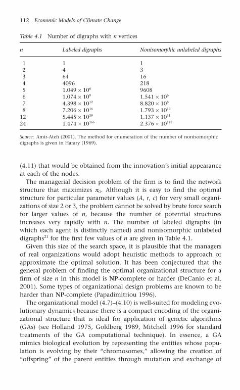
(4.11) that would be obtained from the innovation’s initial appearanceat each of the nodes.

The managerial decision problem of the firm is to find the networkstructure that maximizes pG. Although it is easy to find the optimalstructure for particular parameter values (A, r, c) for very small organi-zations of size 2 or 3, the problem cannot be solved by brute force searchfor larger values of n, because the number of potential structuresincreases very rapidly with n. The number of labeled digraphs (in which each agent is distinctly named) and nonisomorphic unlabeleddigraphs21 for the first few values of n are given in Table 4.1.

Given this size of the search space, it is plausible that the managersof real organizations would adopt heuristic methods to approach orapproximate the optimal solution. It has been conjectured that thegeneral problem of finding the optimal organizational structure for afirm of size n in this model is NP-complete or harder (DeCanio et al.2001). Some types of organizational design problems are known to beharder than NP-complete (Papadimitriou 1996).

The organizational model (4.7)–(4.10) is well-suited for modeling evo-lutionary dynamics because there is a compact encoding of the organi-zational structure that is ideal for application of genetic algorithms(GAs) (see Holland 1975, Goldberg 1989, Mitchell 1996 for standardtreatments of the GA computational technique). In essence, a GAmimics biological evolution by representing the entities whose popu-lation is evolving by their “chromosomes,” allowing the creation of “offspring” of the parent entities through mutation and exchange of


Table 4.1 Number of digraphs with n vertices

n Labeled digraphs Nonisomorphic unlabeled digraphs

1 1 12 4 33 64 164 4096 2185 1.049 ¥ 106 96086 1.074 ¥ 109 1.541 ¥ 106

7 4.398 ¥ 1012 8.820 ¥ 108

8 7.206 ¥ 1016 1.793 ¥ 1012

12 5.445 ¥ 1039 1.137 ¥ 1031

24 1.474 ¥ 10166 2.376 ¥ 10142

Source: Amir-Atefi (2001). The method for enumeration of the number of nonisomorphicdigraphs is given in Harary (1969).

1403_963363_05_cha04.qxd 6/14/2003 11:20 AM Page 112

genetic information (analogous to what happens in biological sexualreproduction), and subjecting the entire population to selection pres-sure over time. In the organizational model, the chromosome is formedby concatenating the rows of the adjacency matrix of the organizationalstructure,

(4.12)

where the element aij of the adjacency matrix equals 1 if the edge (vi, vj) is present and equals 0 if (vi, vj) is absent. For an organization ofsize n, this produces a chromosome of length n2. (In practice, the chromosome length can be reduced to n2 - n because the diagonal ele-ments of AG are all zero and can therefore be omitted.) Fitness of theorganization is determined by its profitability according to equations(4.9)–(4.10). Two members of the evolving population can produce anoffspring by “crossover” exchange of genetic information. This is illus-trated in Figure 4.2 for two parent organizations of size 6.

Parent 1 is the organization shown in Figure 4.1. (Keep in mind thatthe all-zero diagonal of the adjacency matrix has been eliminated inthis representation.) Parent 2 is another size-6 organization. If these twoparents are selected to reproduce, and the single “crossover” point is such that the first 12 genes of parent 1 are combined with the last 18 genes of parent 2 (these are shown in boldface italic type in Figure4.2), the resulting offspring organization is as shown. The GA takes a population of organizations, differentially selects members of the pop-ulation for reproduction according to their relative fitness, creates off-spring by the process illustrated in Figure 4.2, and repeats the steps in each successive generation. In addition, mutations can occur atrandom as genes are switched from 1 to 0 or from 0 to 1 according toa probabilistic rule.

This algorithm simulates natural selection. It allows “experimenta-tion” in the formation of organizational structures because differentpieces of parent organizations can be broken off and rejoined, with theoffspring’s survival dependent on the resulting fitness of the newlyformed structure. Different dynamics can be simulated by changing the

AG ija= [ ]


Parent 1 1 0 0 0 0 0 0 1 0 0 0 0 0 1 0 0 0 1 0 0 1 0 1 1 0 1 0 0 0 0Parent 2 1 1 1 0 0 1 0 1 0 0 0 1 1 0 0 1 0 0 1 0 0 1 0 0 1 1 1 1 0 1

Offspring 1 0 0 0 0 0 0 1 0 0 0 0 1 0 0 1 0 0 1 0 0 1 0 0 1 1 1 1 0 1

Figure 4.2 Chromosomes of two parents and offspring, size 6 organization

1403_963363_05_cha04.qxd 6/14/2003 11:20 AM Page 113

rules of the GA. The rules that were varied in the runs reported belowhad to do with selection for reproduction and whether or not “elite”(high fitness) organizations were preserved from generation to genera-tion. This setup is flexible enough to simulate the evolution of “mixed”populations containing organizations of different size.

4.4.2 Some indicative results

Genetic algorithms are commonly employed to attack difficult opti-mization problems such as the choice of organizational structure. In thepresent context we are interested not so much in finding the best struc-ture, but in the characteristics of populations that are evolving underthe pressures of natural selection. In particular, the goal is to see howvariants of the basic GA technique give rise to populations with differ-ent characteristics. By examining these simulated populations, it maybe possible to imagine how proper specification of the GA rules couldmimic the kinds of populations of firms (varying as to the distributionof productivity or profitability, the size distribution, etc.) that areobserved in the real world.

We begin with a population consisting of S “species” of firms. Thesespecies are defined solely in terms of the size of the firms. (Size is definedas the number of agents making up the firms.) There will be M membersof each species in the initial population, so that the total populationsize is M ¥ S. The parameters of reward, cost, and discount rate (A, c, r)are fixed. Three selection methods will be considered: proportionateselection, tournament selection, and population elite selection.

Population elite selection is the simplest of the three, and correspondsmost closely to the implicit population dynamics of Hannan andFreeman’s classic Organizational Ecology (1989). Under this selectionmethod, every member of the population has an equal probability ofbeing selected for reproduction. For each species subpopulation, form anumber of offspring equal to the size of that subpopulation, choosingthe parents at random without replacement and using two-pointcrossover (which produces two offspring from every pair of parents).22

Combine all these subpopulations (including both parents and off-spring), and select the top 50 percent (as measured by their fitness).Repeat for successive generations. This method amounts to a more orless random formation of new organizations that imitate componentsof existing organizations; however, there is no conscious selection ofthe more successful organizations in a population to imitate. Organiza-tions simply are born and die, with survival determined by relativefitness. Selection pressure operates on the population as a whole.


1403_963363_05_cha04.qxd 6/14/2003 11:20 AM Page 114

Tournament selection is more sensitive to the fitness of the individ-ual organizations in determining whether they reproduce. Beginningwith the existing population, two members are selected randomly (withreplacement). Of the two selected, the one with the higher fitness ischosen as the first parent. After that selection is made, two members ofthe first parent’s species are selected at random, again with replacement.The second parent is the one of this pair with the higher fitness score.The two parents chosen in this way then reproduce via two-pointcrossover with a 50 percent probability. If the crossover does not occur,both parents are copied into the next generation. This method differsfrom population elite selection in that the candidates for parenthoodare chosen in a way that favors the more fit members of the popula-tion. This corresponds to the notion that the newly formed firms tendto imitate elements of the more successful existing firms. The reasonsuch a selection process cannot be assumed to take place, of course, isthat it cannot be assumed that entrants necessarily know the prof-itability of existing firms. On the other hand, if the new organizationsare formed as a result of spinoffs or joint ventures by existing firms, itis plausible that the more successful firms would have a higher prob-ability of engaging in the formation of new firms. Thus, there is no apriori presumption of which selection dynamic is more plausibly areflection of competitive market pressures.

The third selection method, proportionate selection, is similar to tour-nament selection except that the parents are selected for reproductionwith probabilities proportional to their relative fitness in the whole pop-ulation.23 This method is analogous to the “replicator dynamics” thatappears in the literature of evolutionary game theory (Weibull 1995). Itrepresents a different way of favoring the reproduction of the more fitmembers of the population. Indeed, each of these selection methodscan be thought of as selecting population members for reproductionaccording to some probability distribution. Population elite selection is equivalent to using a uniform distribution, tournament selection isequivalent to a distribution based on rank ordering of the fitness scores,and proportionate selection is equivalent to a distribution takingaccount of the relative magnitudes of the fitness scores.

With proportionate or tournament selection, the evolution can takeplace with or without the preservation of population elites. If elites arepreserved, some selected number of the most fit members of the popu-lation are simply copied over from one generation to the next. This pre-vents degradation of highly fit organizations; if the GA has found highlyefficient structures, the preservation of elites prevents those structures


1403_963363_05_cha04.qxd 6/14/2003 11:20 AM Page 115

from being broken up through crossover. On the other hand, even suc-cessful organizations are subject to “reinvention,” internal reorganiza-tion, or change in response to fashions and trends. Thus, runs with andwithout elite preservation were carried out.

A basic question is whether these evolutionary dynamics generatesimilar population distributions, for different runs of the same evolu-tionary mechanism and across the different mechanisms. Consider firstwhether the same mechanism leads to the same distribution of firmsfor different runs. The particular distribution of fitness scores in anyevolutionary run will depend on (1) the initial randomly generated pop-ulation that provides the basic genetic material for evolution of the population, and (2) the (partially) random events that occur during evolution as crossover and mutation take place. Selection pressure willtend to preserve the more fit structures, but the question is whether thedistribution of fitness scores tends to be similar after each evolutionaryrun. This has the same flavor as the question asked in connection withbiological evolution, “What would be conserved if the tape were playedtwice?” (Gould 1989, Fontana and Buss 1994).

Figure 4.3 shows typical histograms24 of the fitness scores of two populations evolved under these conditions: firm size 15, populationsize 500; 10 elite firms saved each generation; crossover probability 0.5;mutation probability (1/210); (A, c, r) = (500, 3.5, 0.1); maximum timesteps for diffusion of the profitable innovation = 10. The evolution wasallowed to continue for 500 generations, and proportionate selectionwas the GA type. The first thing to observe from Figure 4.3 is that thereis a considerable spread in fitness scores. Even after 500 generations, thebulk of the population falls short of the maximum fitness score achievedby the most profitable organizations. Most of the firms in the evolvedpopulations are clearly not optimized even after 500 generations. It isalso evident that the distributions are skewed to the left. This patternis reasonable because, while selection pressure will promote the survivalof the more fit members of the evolving population, the processes ofcrossover and mutation will at the same time give rise to quite a fewfailed experiments in organizational structure in every generation. Thisis akin to the stylized fact that in the real world most new firms failrather quickly; the rule of thumb is that four out of five new small businesses fail in the first five years of their life.

It is also the case that even for a common set of parameters and a particular GA, the evolved populations do not all exhibit the same distribution of fitness scores. There are a number of statistical tests forwhether a group of samples all come from the same distribution. The


1403_963363_05_cha04.qxd 6/14/2003 11:20 AM Page 116

most common is the one-way analysis of variance (ANOVA). However,ANOVA requires that the underlying distribution(s) be normal, and weknow that this is not likely to be the case for the fitness scores of eitherthe evolved populations or the original random populations. The fitnessfunction is not the sum of a large number of small independent dis-turbances; it is highly nonlinear in the out-degree of the vertices(because of the functional form of the cost). Furthermore, the effects ofthe connections between vertices are not independent influences ontotal fitness; removal of a single edge can drastically change the fitness


0

20

40

60

80

100

–16 000 –12 000 –8000 –4000 0 4000

Series: POP01Sample 1 500Observations 500

Mean 124.2437Median 810.9670Maximum 3980.470Minimum –18 430.90Standard deviation 2852.717Skewness –1.698058Kurtosis 8.002722

Jarque-Bera 761.6840Probability 0.000000

0

20

40

60

80

100

120

–16 000 –12 000 –8000 –4000 0 4000

Series: POP02Sample 501 1000Observations 500

Mean 36.89054Median 840.1670Maximum 4025.110Minimum –17 668.50Standard deviation 3082.862Skewness –1.908422Kurtosis 9.403753

Jarque-Bera 1157.841Probability 0.000000

Figure 4.3 Typical histograms of fitness scores from evolved populations

1403_963363_05_cha04.qxd 6/14/2003 11:20 AM Page 117

of the whole organization if, for example, that edge is necessary to makethe organization fully connected.25

Even though ANOVA is not suitable for testing whether the popula-tion fitness scores of different evolutionary runs come from the samedistribution, a nonparametric test such as the Kruskal–Wallis test isappropriate. In this nonparametric version of the analysis of variance,each evolved population is treated as a sample. One hundred evolu-tionary runs of each variety of GA were carried out, and each popu-lation had 500 organizations. These 50,000 observations were thenranked, and the rank sums computed for each sample (run). If there areK samples with rank sums R1, R2, . . . , RK, and ni observations in eachsample (with n observations in all), the Kruskal–Wallis statistic is

(4.13)

The distribution of this statistic is well-approximated by the c2 distribu-tion with (K - 1) degrees of freedom (Newbold 1995; see also the dis-cussion in Siegel 1956). Table 4.2 displays the Kruskal–Wallis statisticsand their associated probability values under the null hypothesis thatall 100 populations have the same distribution of fitness scores for eachGA. Both the original populations and the evolved populations after500 generations were tested. It is clear from Table 4.2 that in no casecan the null hypothesis of all populations belonging to the same fitnessdistribution be rejected at the 5 percent level for the original popula-tions, while in the evolved populations the null hypothesis can berejected in every case with only a miniscule probability of Type I error.This result holds whichever evolutionary mechanism is in operation.26

These statistical results are strong, but the economic implications areof equal significance. Even though the initial populations are statisti-cally indistinguishable (in terms of the distributions of the fitness scoresof the firms), the evolved populations show fitness distributions that arequite definitely distinct. This holds even for uniform evolutionary andenvironmental conditions – the same GA, firm size, and cost, benefit,and discount rate parameters. The evolutionary process is “open-ended”in that the fitness distribution of firms is not determined by the under-lying parameters and the dynamic selection mechanism. This meansthat random events or historical accidents can measurably affect theoutcome of the process. There is nothing new about such a characteri-zation of evolution – after all, biological evolution has selected forlocomotion by creatures with 1, 2, 4, 5, 6, 8, and “many” legs. Just asthere is no single evolutionary outcome for the “equilibrium” number

Wn n

Rn

ni

ii

K

=+( )

- +( )=Â12

13 1

2

1


1403_963363_05_cha04.qxd 6/14/2003 11:20 AM Page 118

of appendages of life forms, there can be no presumption that any par-ticular distribution of efficiencies of firms (including the distributionthat happens to exist at the present time) represents an “equilibrium.”An obvious consequence is that policy interventions might, by chang-ing the initial conditions or injecting new information into the market,influence the evolutionary path of the population of firms.

A second kind of question has to do with whether, in cases in whichthe initial population contains firms of different species, the evolu-tionary process always tends to lead to the dominance of one type offirm. The dynamics of interspecies competition can be much more com-plicated than it might seem. Figure 4.4 shows the number of each ofthe three species (firms of size 15, 16, and 17) remaining in the popu-lation (total population size 1500) at the end of each generation for a particular set of parameters and one evolutionary dynamic. In Fig-ure 4.4, the dashed line represents the number of size 15 firms in the


Table 4.2 Tests of null hypothesis that all 100 populations are from the samefitness distribution

GA Firm size Initial generation 500th Generation

Kruskal– Probability Kruskal– ProbabilityWallis value Wallis value

ps, no elites 15 91.808 0.683 4482.200 ~0ps, no elites 16 97.225 0.532 5036.137 ~0ps, no elites 17 106.407 0.287 9253.005 ~0

ps, elites 15 121.749 0.060 1425.642 ~0ps, elites 16 93.625 0.633 1343.897 ~0ps, elites 17 107.779 0.257 1187.104 ~0

ts, no elites 15 87.883 0.780 2665.949 ~0ts, no elites 16 113.901 0.145 2156.114 ~0ts, no elites 17 77.568 0.945 3016.906 ~0

ts, elites 15 75.729 0.960 787.931 ~0ts, elites 16 72.323 0.980 880.114 ~0ts, elites 17 74.281 0.970 662.428 ~0

pe 15 108.350 0.245 49946.71 ~0pe 16 81.337 0.902 49968.05 ~0pe 17 90.272 0.723 49683.87 ~0

Source: See text. ps = proportionate selection; ts = tournament selection; pe = populationelite selection. Kruskal–Wallis statistics distributed as c2 with 99 degrees of freedom.

1403_963363_05_cha04.qxd 6/14/2003 11:20 AM Page 119

population, the dotted line the number of size 16 firms, and the solidline the number of size 17 firms. It can be seen that the number of thesize-17 species drops off precipitously in the first 50 generations, butrecovers between the 130th and 230th generations (approximately).There is a stretch of time during this interval when there are more size-17 firms than either of the other two types. However, at around the250th generation, the number of size-17 firms begins to drop again,until by about the 340th generation these firms have disappeared fromthe market (the size-17 species has become extinct). After this point,there seem to be about twice as many size 15 firms as size 16 ones. Isthis an “equilibrium”? However one might be inclined to answer thatquestion, what is clear is that looking at only a single moment in timecould give an entirely misleading impression of the “equilibrium” size


0

200

400

600

800

1000

1200

14001 21 41 61 81 101

121

141

161

181

201

221

241

261

281

301

321

341

361

381

401

421

441

461

481

Generation

Nu

mb

er

Figure 4.4 15 vs 16 vs 17 proportionate selection with no elites and type 1scaling

1403_963363_05_cha04.qxd 6/14/2003 11:20 AM Page 120

distribution of firms. If this industry were examined at the time whenthe size-17 firms were the most common species, there would be noindication that these firms would eventually be wiped out in competi-tion with the others.

Figure 4.4 gives the result of only one head-to-head competition. Tosee if there are any patterns in repeated runs, Table 4.3 summarizes theresults of 100 such competitions for different versions of the GA. Table4.3 shows that different outcomes can come about for different evolu-tionary runs, and that the relative frequency of the different outcomesalso depends on the selection mechanism at work. In these runs, theinitial population is always equally divided among the three species offirms, and the exogenous parameters (benefit, cost, and discount rate)are identical. The fact that not all the runs with the same selectionmechanism come out the same means that pure chance and/or theinitial conditions play a role in the outcome. This is the multispeciesanalogue to the result shown in Table 4.2 that the evolved populationsdiffer under identical dynamics in single-species evolutions. The initialconditions may matter because each run begins with a different popu-lation of randomly generated organizations. “Path dependence”27 mayalso be playing a role because each generation takes as its starting pointthe population that had evolved through the previous generation, butthe evolutionary outcome is not purely path-determined because ofrandom crossover and mutation that occur along the way.

When proportionate selection with no elites is the evolutionarymechanism, the size-17 firms become extinct about 35 percent of thetime. They never dominate the population completely. Only 4 of the100 runs result in only one species remaining. Most of the runs windup with a mix of species, predominantly size-15 and size-16 firms. Onthe other hand, when elites are preserved the proportionate selectionruns always lead to a population containing only one species, althoughwhich species dominates is a matter of chance (15 percent of the timeit is the size-15 firms, 41 percent of the time size-16, and 44 percent ofthe time size-17). While no elites tends to favor the smaller firms, thepreservation of elites favors the larger firms.

If tournament selection is employed, the size-15 firms are almostalways eliminated. This form of selection pressure produces populationsconsisting exclusively of one type of firm, most frequently the size-17species. Nevertheless, between about a quarter and a third of the runsresult in the extinction of the size-17 firms. Once again, chance plays a role in the final composition of the market. Yet for the fixed set of (A, c, r) parameters, there is one size and organizational structure that


1403_963363_05_cha04.qxd 6/14/2003 11:20 AM Page 121


Table 4.3 Results of head-to-head competition, 3 species, 100 runs of 500 gen-erations each, A = 500, c = 3.5, r = 0.1

Frequency range Proportionate selection

No elites Elites

Size 15 Size 16 Size 17 Size 15 Size 16 Size 17

0 2 12 35 85 59 561–250 0 22 35 0 0 0

251–500 7 37 22 0 0 0501–750 18 23 6 0 0 0751–1000 33 2 1 0 0 0

1001–1250 12 1 1 0 0 01250–1499 13 0 0 0 0 01500 3 1 0 15 41 44

Tournament selection

No elites Elites


0 92 69 39 98 76 261–250 0 0 0 0 0 0

251–500 0 0 0 0 0 0501–750 0 0 0 0 0 0751–1000 0 0 0 0 0 0

1001–1250 0 0 0 0 0 01250–1499 0 0 0 0 0 01500 8 31 61 2 24 74

Population elite selection

Crossover probability = 0.5 Crossover probability = 1.0


0 100 100 0 100 88 121–250 0 0 0 0 0 0

251–500 0 0 0 0 0 0501–750 0 0 0 0 0 0751–1000 0 0 0 0 0 0

1001–1250 0 0 0 0 0 01250–1499 0 0 0 0 0 01500 0 0 100 0 12 88

Source: See text.

1403_963363_05_cha04.qxd 6/14/2003 11:20 AM Page 122

has the highest profitability; it is just that the competitive process is notlikely to find it.

Under population elite selection, all the runs result in completetakeover of the population by only one species. If the crossover proba-bility is 0.5, the size-17 species always wins the competition. (Recall that the crossover probability is the probability of exchange of geneticinformation when two parents are selected for reproduction.) When theparents always “mate” (crossover probability equal to one), the size-17firms usually drive out the other species, but occasionally (12 percentof the time) size-16 species prevail over the other types.

Thus, for identical environmental parameters, the evolutionary selec-tion mechanism can lead to virtually any outcome in the interspeciescompetition. Sometimes one species predominates, and sometimes amix of species remains in the population. In the cases in which onespecies predominates, it can be a different species depending on the run,even with the same selection mechanism. These simulation experimentsdemonstrate the open-endedness of the evolutionary process.


These examples illustrate the principal underlying feature of these evo-lutionary models: the state of an evolving population at any point intime is not uniquely determined. Different dynamic selection mecha-nisms can give rise to populations with different properties, both as tothe size distribution of firms and the distribution of the fitness (prof-itability or efficiency) of firms. In addition, any given evolutionary algo-rithm can lead to populations of firms that differ in size compositionand fitness scores. While some systematic tendencies may be observed,the variety of outcomes is sufficiently large as to preclude sharp char-acterizations of the “end-state” populations. Of course, evolution is nota teleological process, so there is no “end-state” in reality. The term isused here to indicate the evolved population that happens to exist atthe present time. Nevertheless, confusion between the existing popula-tion and some sort of “optimum” is deeply embedded in the “profitmaximization subject to the production function” modeling style.

These findings are consistent with other evolutionary models builtalong similar lines. For example, Amir-Atefi (2001) shows that becausethe search space in seeking the optimal organizational form is so large,firms that adopt a “rule of thumb” to explore only over team-basedstructures can frequently outcompete firms whose strategy is to searchover the entire space, even though the team-based forms are perforce


1403_963363_05_cha04.qxd 6/14/2003 11:20 AM Page 123

suboptimal. Mitchell (2001) shows how an evolutionary process bywhich agents choose their degree of connectedness may or may not leadto optimal network configurations, depending on the initial conditionsand the property-rights features of the costs and benefits of technologyadoption. In a model that specifies firms carrying out two distinct tasks(one corresponding to the adoption of a profitable technology, as inequations (4.7)–(4.10), and an abstract version of assembly), DeCanioet al. (2001) show that an evolutionary process leads to a range of effi-ciency levels, and that organizations having very different structures canshow comparably high efficiency levels. All of these models representcomponents of a research program of “computational organizationaldemography” based on evolutionary dynamics.28

This perspective provides a clear scientific rationale for why firmsexhibit a range of efficiency characteristics. The differences originate in the nature of the dynamic market selection process itself. In the neoclassical formulation, it is difficult to see why many or most firmsappear to be operating inside their production-possibilities frontiers.The attempt to preserve the optimization paradigm by invoking unob-served “transactions costs” that account for the deviations from opti-mality is unconvincing. It is also unscientific, because there is noevidence that could falsify the hypothesis – by construction the trans-actions costs are unobservable. The evolutionary model proposed here,on the other hand, is computationally grounded and entirely transpar-ent. It does have the implication, however, that knowing the charac-teristics of the population of firms (in any particular industry or acrossindustries) today is not in general sufficient to deduce the evolutionarymechanism that gave rise to it – the same mechanism can lead to different populations, and the same population may be the outcome ofalternative evolutionary mechanisms.

One clear implication is that there should be no presumption that the existing technology choices, resource allocations, size distribu-tions of firms in industries, or internal decision-making practices offirms are optimized. Of course, this is just the same conclusion as thatreached by the modern theory of the firm, and supported by the evi-dence, as discussed in section 4.2. A number of policy conclusionsfollow:

• Initial conditions, particular historical contingencies, and strategicpolicy interventions may affect the technologies and organizationalforms used in production without having any adverse effect onoverall economic efficiency;


1403_963363_05_cha04.qxd 6/14/2003 11:20 AM Page 124

• The possibility that firms (and the economy as a whole) may beinside their production-possibilities frontiers means that there is not necessarily a trade-off between environmental protection (mani-fested by, for example, a reduction in greenhouse gas emissions) andimprovements in productivity or profitability as conventionally measured;

• The range of effective policy instruments is much broader than whathas traditionally been considered in the climate debate. In additionto taxes (or tradable permits) and command-and-control regulations,environmental objectives may reasonably be pursued by voluntaryprograms, campaigns to increase the salience of environmentalvalues, government demonstration projects, and facilitation of inter-firm and interpersonal networking.29

Just as in the case of the representation of consumer demand, the representation of production in the prevailing integrated assessmentmodels abstracts from essential features of the phenomena beingmodeled. The models that have been used to predict the effects ofclimate protection policies set up their production sectors in such a wayas to preclude much of the variation and potential for change that is infact an essential part of industrial reality in a market economy. By ignor-ing such vital facts as the variance in efficiency of firms, the integratedassessment models violate standards of scientific practice. In contrast,the evolutionary perspective shows how, within the requirements forinternal consistency and computability, dynamic models can exhibitthe kind of open-endedness that actually characterizes the real world.


1403_963363_05_cha04.qxd 6/14/2003 11:20 AM Page 125

5The Forecasting Performance ofEnergy-Economic Models

126

5.1 Introduction

The predictive performance of economic-energy models has a directbearing on their usefulness in the climate policy debate. One of thesalient aspects of that debate is that some opponents of action to reduceGHG emissions are willing to make confident assertions about what the “cost to the economy” of various policy proposals (such as com-pliance with the Kyoto Protocol) would be. Yet at the same time theseskeptics doubt the validity of the science that underlies forecasts ofglobal warming, and claim that the observed century-long trend ofincreasing temperatures is indistinguishable from the “noise” of naturalvariation. They are willing to base strong policy recommendations onthe forecasts of economic/energy models that purport to predict out-put, employment, prices, and emissions decades into the future, whiledenying the predictive power of physical science models of climatedynamics.

Such a perspective might be understandable if the foundations of theeconomic models were solidly established while those of the atmos-pheric and geophysical models were speculative. The truth, however, isjust the opposite: the physical and chemical foundations of atmosphericgeneral circulation models (GCMs) are firmly grounded in experimen-tally verified theory – the kind of theory that predicts that airplanes canfly, that green plants will convert CO2 to cellulose and oxygen throughphotosynthesis, and that heat flows from regions of higher temperatureto regions of lower temperature in closed systems. On the other hand,as demonstrated in Chapters 2–4, the economic models that are thesource of pessimistic predictions about the cost of emissions reductionsare dependent on unverified (or, in some cases, false) assumptions

1403_963363_06_cha05.qxd 6/14/2003 11:21 AM Page 126

about how firms and individuals behave, unexamined ethical judg-ments about the relationship between present and future generations,and implicit welfare criteria that inordinately favor the status quo. Inother words, those who would put off dealing with climate change areskeptical of science that is fundamentally sound, but uncritically accepteconomics that is theoretically, empirically, and ethically questionable.

Despite the weaknesses of integrated assessment models that havebeen detailed in the previous chapters, it is still possible that thosemodels might be useful in climate policy analysis if they do a good jobof forecasting either the future course of the economy (including energysupply, demand, and prices) and/or they offer reliable guidance aboutthe quantitative effects of various policy alternatives. Even if the theo-retical foundations of the models are suspect, they might still serve asforecasting “black boxes” or as a means of calculating policy scenarios.There is, after all, a strand of economic theory that claims that it doesnot matter whether firms really do maximize profits or not, or whetherconsumers maximize well-defined utility functions subject to a budgetconstraint; it is enough that the firms and consumers act “as if” theydo so. This approach to predictive analysis was articulated perhaps mostclearly by Milton Friedman in his Essays in Positive Economics (1953).

Friedman’s approach has been criticized elsewhere (Simon 1963,Laitner et al. 2000; see also the discussion of evolutionary models inChapter 4). Suffice it to say that the “as if” hypothesis rests on strongpresumptions about the underlying dynamics of the economic system,presumptions that have neither been established nor tested. Friedmanappeals to an evolutionary argument (if the firms did not act “as if” theymaximized profits, they would be driven out of business) that is not a necessary feature of real evolutionary processes. Evolution may exertpressure in the direction of greater efficiency, but it is a nonteleologicalmechanism that typically allows room for continuous improvement.But even if the “forecasting black box” conception of energy/economicmodels were acceptable in theory, we would still want to know if themodels offer accurate forecasts in practice. In order to place any confi-dence in the models’ predictions of policy effects, we would want toknow what their record has been in the past.

5.2 The long-term predictive power of economic models is limited

Anthropogenic climate change is a process that unfolds on time scalesmeasured in decades. Economists since Malthus have understood that

The Forecasting Performance of Energy-Economic Models 127

1403_963363_06_cha05.qxd 6/14/2003 11:21 AM Page 127

it is important to think about the long run. But thinking systematicallyabout (and gaining insights into) the long run and the factors that shapeit – technological progress, stable institutions and property rights, etc.(Solow 1970, Rosenberg and Birdzell 1986, Lucas 1988, Barro and Sala-i-Martin 1995) – is quite different from making detailed predictionsabout specific economic variables such as the rate of growth, employ-ment, the price level, or the relationship of any particular sector orindustry (such as energy) to the economy as a whole. And when it comesto long-term forecasting, as distinct from acquiring insight regardinglong-term economic processes, the fact is that there simply are no eco-nomic models that have a track record of success.

Some forecasting exercises are held in deservedly low regard becauseof their pessimistic claims regarding resource exhaustion. A few envi-ronmentalists and others who have been concerned with global resourceissues have contributed their share of exaggerations and inaccurate fore-casts.1 For example, the Club of Rome’s notorious warning, The Limitsto Growth (Meadows et al. 1972), gave wide publicity to a set of esti-mates made by the US Bureau of Mines projecting the “Static Index” (inyears) of a variety of “nonrenewable natural resources.” The Static Indexwas defined as “the number of years known global reserves will last atcurrent global consumption” (US Bureau of Mines 1970). It was perhapscomforting to project in 1970 that there were sufficient reserves of coalto last 2300 years, and that reserves of aluminum, chromium, cobalt,iron, and the platinum group all exceeded 100 years. However, the StaticIndex values of the years of remaining reserves for gold (11 years), lead(26 years), mercury (13 years), silver (16 years), tin (17 years), and zinc(23 years) were such that, if the forecasts had been accurate, the worldwould be using exclusively recycled quantities of these metals by now.The Static Index of petroleum was 31 years, so that the 1970 forecast ofthe date at which we would have “run out of oil” was 2001.

Furthermore, there is a disconnection between the way the policydebate on climate change is dominated by economic models and fore-casts, and the relative lack of influence of such techniques in busi-ness management. Few companies today maintain substantial economicforecasting units, and a wide spectrum of general business and eco-nomic forecasts can be obtained at relatively low cost. For example, a12-month subscription to Blue Chip Economic Indicators, which containsthe forecasts of more than 50 leading business economists (or their com-panies) of economic growth, inflation, interest rates, and other impor-tant economic variables, could recently be purchased for $627 per year(Moore 2002).2 Although most of the information contained in Blue


1403_963363_06_cha05.qxd 6/14/2003 11:21 AM Page 128

Chip Economic Indicators pertains to the short run (one to two years),longer-run forecasts (for five years annually and then an average for fiveadditional years) are also presented. These longer-run projections comewith a disclaimer, however: “APPLY THESE TREND PROJECTIONS CAUTIOUSLY.The vast majority of economic and political forces cannot be evaluatedover such a long time span” (Moore 2002, p. 14, capitalization in theoriginal).

The poor track record of energy forecasting is hardly a secret. In arecent comprehensive survey paper on the “perils and promise of long-term forecasts,” Koomey et al. (2001) provide numerous examples offorecasts that failed to be realized, from Jevons’ gloomy nineteenth-century assessment of the future of England’s energy system (which wascoal-based at the time Jevons wrote) to long-term forecasts of US energydemand made during the 1970s (actual consumption by 2000 hasturned out to be at the very lowest end of the range of the forecasts).Their advice to forecasters is “be modest; the future will probably unfoldin ways that you haven’t dreamed” (p. 2). A recent issue of The Econo-mist (November 3, 2001), in an article describing controversy over the“Hubbert curve” (the pattern of oil production and decline originallyput forward by Shell geologist M. King Hubbert) asked,

Who is right? In making sense of these wildly opposing views, it isuseful to look back at the pitiful history of oil forecasting. Doomstershave been predicting dry wells since the 1970s, but so far the oil isstill gushing. Nearly all the predictions for 2000 made after the 1970soil shocks were far too pessimistic. America’s Department of Energythought that oil would reach $150 a barrel (at 2000 prices); evenExxon predicted a price of $100. (p. 81)

This kind of skepticism is a reflection of the ineffectiveness of eco-nomic forecasting models, but there is a deeper reason at work as well.Specific, detailed knowledge about future economic trends or fluctua-tions could be converted into enormous wealth. For example, the abilityto predict movements in the stock market on a daily, weekly, monthly,or yearly basis would enable the possessor of such information to amasshuge gains from speculation. The existence of such potential gainswould draw entrants, who would compete against each other in exploit-ing the sources of information about the future. The market positionstaken by the agents with knowledge of the future would cause the trendsthat were the source of the speculative profits to disappear, and theextraordinary gains from speculation would be reduced to normal levels


1403_963363_06_cha05.qxd 6/14/2003 11:21 AM Page 129

of profit from arbitrage and market research. This is the essential insightof the “efficient markets” idea that has come to dominate the economictheory of financial markets. The conclusion is that most fluctuations ineconomic variables cannot in principle be predicted. What is true aboutstock prices is true also about commodity prices – oil and natural gasno less than gold or pork bellies. The general proposition is that marketcompetition tends to squeeze out opportunities for speculative profits,and hence that reliable knowledge of future economic variables is verydifficult if not impossible to come by.

It is important to realize that the policy relevance of energy-economicmodels depends on their ability to project both prices and quantities ofthe various forms of energy used by the economy. The quantities of thevarious kinds of primary energy used determine GHG emissions, andthe prices of energy are important in determining economy-wide effects.The models typically specify the impact of policy instruments (carbontaxes or energy taxes, cap-and-trade permit systems, etc.) through speci-fication of price changes, so the sensitivity of the models to energy pricechanges is a key component of the analysis. It is well-known that the“baseline” forecasts for prices and quantities are both the starting pointand a major determinant of the results of any analysis of these market-oriented policies (Weyant 2000). This chapter will explore how suc-cessful economic-energy models have been in predicting energy prices,quantities, or both.

5.2.1 History of economic forecasts using energy-economy models

Because most GHG emissions arise from the use of fossil fuels to produceenergy services, economic forecasting for climate policy has to start withthe energy sector. Forecasting of energy demand and usage became anacademic subspecialty during the oil price shocks of the 1970s. Theimpact of those price disruptions spawned a great deal of interest inmodeling that was designed to predict the energy future of the UnitedStates and the rest of the world. In looking at the record of the modelsthat were built during the 1970s to forecast the course of energy demandand prices, one finds that the forecasting performance of energy/economic models has not been accurate enough to justify their use inmaking policy judgments. Indeed, judging from their history, the rangeof uncertainty in the forecasts of the best models typically is greater than the changes in energy demand that are the subject of the current climate policy debate.

It should be noted that in order to do a retrospective analysis of the


1403_963363_06_cha05.qxd 6/14/2003 11:21 AM Page 130

performance of forecasting models it is necessary to use published fore-casts that are old enough to make the forecasting exercise interesting.Simply predicting that next year will look much like this year is unlikelyto be wrong by more than a few percentage points; but the time scalerelevant to climate modeling has to span a number of decades at least.Forecasting techniques may improve over time, so the retrospectiveanalysis cannot ascertain the predictive power of current models. Thisdoes not mean that the retrospective approach sheds no light on theperformance of current models, however. In some cases (such as theNational Energy Modeling System (NEMS) used by the Energy Infor-mation Agency of the US Department of Energy to construct the AnnualEnergy Outlook (AEO) forecasts), the improvements have been in-cremental rather than revolutionary. Notwithstanding the potentialadvances in modeling technique, it is worth bearing in mind that the models examined below were considered to be “state of the art” fortheir time. The record of forecasting models in general can at aminimum provide grounds for caution in accepting the claims of cur-rent forecasts.

Academic and government studies of the accuracy of forecasts whencompared to the actual performance of the energy sector show that theforecasts have a dismal record. It should be noted at the outset that thisis not meant to be in any way a criticism of the forecasters themselves;indeed, these scholars and analysts are part of the best tradition of social scientific research. Their results have been published in the peer-reviewed or monographic literature, or in reports that are available forscientific review. The point is that even when the best representativesof the modeling community are examined regarding the accuracy oftheir forecasts, there is very little justification for optimism about long-term economic forecasting ability.

An early comprehensive study of the reliability of forecasting isWilliam Ascher’s Forecasting: an Appraisal for Policy-Makers and Planners(1978). Ascher examined the accuracy of predictions in a number ofareas, including population, (macro)economics, energy, transportation,and technological forecasting. In one set of comparisons, Ascher lookedat the accuracy of energy forecasts with target dates up to 1970 and withtarget date of 1975 for three categories: total energy demand, electric-ity generated, and petroleum consumption. His results are interestingin part because the pre-1970 target date forecasts were made in theperiod before the first of the oil price shocks while the target date of1975 occurred after this shock. Ascher found (not surprisingly) that for


1403_963363_06_cha05.qxd 6/14/2003 11:21 AM Page 131


the target dates of 1970 and earlier, the forecasts became more accuratethe shorter the forecast period. Nevertheless, the errors were still large.For electricity consumption, the median error of 15-year forecasts wasabout 13 percent, compared to 6 percent for 10-year forecasts and 3.5percent for 5-year forecasts. The 15, 10, and 5-year median forecasterrors for petroleum were as large or larger: 13, 10, and 6 percent respec-tively. Not enough total energy forecasts were made with a pre-1975target date to allow meaningful comparisons (Ascher 1978, 101ff.).

Even more instructive is Ascher’s collection of 5- and 10-year forecastshaving target years of 1980 and 1985, for each of the three energy categories. Although Ascher found “no indication yet of improvedmethodology in forecasting energy demand,” he did state that “the onlyglimmer of hope for better forecasts in the future is the performance ofthe . . . econometric energy models” (1978, pp. 125–6). (His optimismmay have been misplaced, as will be seen below.) Table 5.1 reproducesthe forecasts in three energy categories, along with the actual values ofeach of the energy quantities and the percentage error for each of theforecasts. It should be noted that the forecasts reported by Ascher arein some cases median or average forecasts from the studies cited, so thatthe actual range of forecast errors would be greater than that computedin Table 5.1. The average absolute percentage errors for 1985 range from30 percent (for petroleum consumption) to 48 percent (for total energydemand). The 1980 average absolute percentage errors are smaller, butstill substantial.

A significant improvement in the sophistication and theoreticalgrounding of long-term energy forecasts is represented by William Nordhaus’ (1979) monograph, The Efficient Use of Energy Resources. Thisstudy is notable because it very definitely represented the “state of theart” of energy modeling at its time. The model design and implemen-tation are informed by economic theory, carefully estimated elasticitiesof demand for energy in different sectors, and the best engineering esti-mates of costs and supply availability. The models are unified in an opti-mizing programming framework, and the forecasts were constructedusing the most sophisticated numerical methods that were available inthe 1970s. In short, The Efficient Use of Energy Resources exemplifies thehighest standards of applied economic practice at the time.

Even so, Nordhaus’ longer-term forecasts of energy prices and con-sumption missed the mark by a considerable margin. One of the chiefconcerns of his monograph was appraisal of the extent of OPEC’smonopoly power in the world oil market, so Nordhaus calculated threekinds of oil price forecasts: the “efficient” price path corresponding to

1403_963363_06_cha05.qxd 6/14/2003 11:21 AM Page 132

The Forecasting Perform

ance of Energy-Economic M

odels133

Table 5.1 Actual energy usage compared to 1974–76 forecasts (Ascher 1978)

Source Total energy demand Electricity generated by utilities Petroleum consumption (1015 BTU/yr) (109 kWhr/yr) (106 bbl/yr)

% % % % % %1980 error 1985 error 1980 error 1985 error 1980 error 1985 error

Actual value 76a 74a 2286 2470 6225 5740

Shell Oil 83 9 98 32 – – – 8300 33 8030 40FEAb – – 99 34 2574 13 3348 36 – – 7556 32FEAc 87 14 102 38 – – 3990 62 6077 -2 7423 29Bureau of Mines 87 14 104 41 2769 21 3960 60 7433 19 8375 46Data Resources, Inc. 90 18 106 43 2589 13 3383 37 7099 14 8158 42Ford Foundation 92 21 107 45 – – – – 6789 9 5475 -5

Energy Policy ProjectJohn Gray/NUS, Inc.b – – 113 53 – – 3604 46 – – – –OECDc 97 28 114 54 3042 33 4207 70 6855 10 7556 32AEC – – 118 59 – – – – – – – –John McKetta/ 107 41 138 86 – – – – – – – –

University of TexasWestinghouse – – – – 2516 10 3211 30 – – – –Joskow and – – – – 2514 10 3217 30 – – – –

Baughman/MITb

Oak Ridge National – – – – 2530 11 3245 31 – – – –Laboratory

1403_963363_06_cha05.qxd 6/14/2003 11:21 AM Page 133

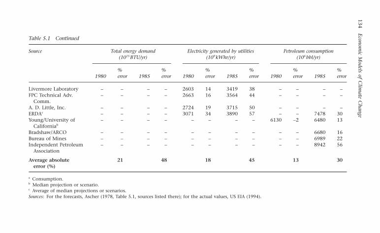
134Econom

ic Models of C

limate C

hange

Table 5.1 Continued

Source Total energy demand Electricity generated by utilities Petroleum consumption (1015 BTU/yr) (109 kWhr/yr) (106 bbl/yr)

% % % % % %1980 error 1985 error 1980 error 1985 error 1980 error 1985 error

Livermore Laboratory – – – – 2603 14 3419 38 – – – –FPC Technical Adv. – – – – 2663 16 3564 44 – – – –

Comm.A. D. Little, Inc. – – – – 2724 19 3715 50 – – – –ERDAc – – – – 3071 34 3890 57 – – 7478 30Young/University of – – – – – – – – 6130 -2 6480 13

Californiab

Bradshaw/ARCO – – – – – – – – – – 6680 16Bureau of Mines – – – – – – – – – – 6989 22Independent Petroleum – – – – – – – – – – 8942 56

Association

Average absolute 21 48 18 45 13 30error (%)

a Consumption.b Median projection or scenario.c Average of median projections or scenarios.Sources: For the forecasts, Ascher (1978, Table 5.1, sources listed there); for the actual values, US EIA (1994).

1403_963363_06_cha05.qxd 6/14/2003 11:21 AM Page 134

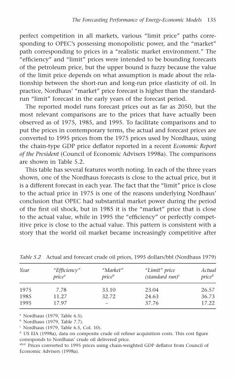
perfect competition in all markets, various “limit price” paths corre-sponding to OPEC’s possessing monopolistic power, and the “market”path corresponding to prices in a “realistic market environment.” The“efficiency” and “limit” prices were intended to be bounding forecastsof the petroleum price, but the upper bound is fuzzy because the valueof the limit price depends on what assumption is made about the rela-tionship between the short-run and long-run price elasticity of oil. Inpractice, Nordhaus’ “market” price forecast is higher than the standard-run “limit” forecast in the early years of the forecast period.

The reported model runs forecast prices out as far as 2050, but themost relevant comparisons are to the prices that have actually beenobserved as of 1975, 1985, and 1995. To facilitate comparisons and toput the prices in contemporary terms, the actual and forecast prices areconverted to 1995 prices from the 1975 prices used by Nordhaus, usingthe chain-type GDP price deflator reported in a recent Economic Reportof the President (Council of Economic Advisers 1998a). The comparisonsare shown in Table 5.2.

This table has several features worth noting. In each of the three yearsshown, one of the Nordhaus forecasts is close to the actual price, but itis a different forecast in each year. The fact that the “limit” price is closeto the actual price in 1975 is one of the reasons underlying Nordhaus’conclusion that OPEC had substantial market power during the periodof the first oil shock, but in 1985 it is the “market” price that is closeto the actual value, while in 1995 the “efficiency” or perfectly compet-itive price is close to the actual value. This pattern is consistent with astory that the world oil market became increasingly competitive after


Table 5.2 Actual and forecast crude oil prices, 1995 dollars/bbl (Nordhaus 1979)

Year “Efficiency” “Market” “Limit” price Actual pricea priceb (standard run)c priced

1975 7.78 33.10 23.04 26.571985 11.27 32.72 24.63 36.731995 17.97 – 37.76 17.22

a Nordhaus (1979, Table 6.5).b Nordhaus (1979, Table 7.7).c Nordhaus (1979, Table 6.5, Col. 10).d US EIA (1998a), data on composite crude oil refiner acquisition costs. This cost figurecorresponds to Nordhaus’ crude oil delivered price.abcd Prices converted to 1995 prices using chain-weighted GDP deflator from Council ofEconomic Advisers (1998a).

1403_963363_06_cha05.qxd 6/14/2003 11:21 AM Page 135

OPEC’s heyday, but that would mean that a political forecast of thestrength and cohesiveness of the OPEC countries over time would havebeen crucial to forecasting the actual path of oil prices over the decadeand a half following publication of The Efficient Use of Energy Resources.The book itself contains no such political analysis.

There is a second difficulty with these forecasts. The Nordhaus modelis an integrated model that forecasts both prices and quantities ofenergy. The lower the price that is forecast, the higher is the forecastquantity consumed. In the case of the Nordhaus model, the actual con-sumption of energy is lower than any of the forecast values for the post-1979 years. This is illustrated in Table 5.3. As can be seen from this table,the “market” projection for 1975 is close to actual consumption, but inthis case the model’s price is 25 percent too high. In 1985, the modelerrors in forecasting total quantity are 17 percent for the “market” fore-cast and 37 percent for the “efficiency” forecast; in 1995 these errors are 7 and 29 percent, respectively. Of course, what happened is that the Nordhaus model (and most other forecasts) did not anticipate theunprecedented increase in output per unit of energy that took placeduring the late 1970s and 1980s following the oil shocks. This is so eventhough the Nordhaus model carefully estimated price elasticities for thevarious energy-using sectors based on historical data.

Other energy projections of the 1970s and 1980s overestimated boththe growth in consumption of energy in the United States and thefuture level of energy prices. In an influential article in Foreign Affairs,Amory Lovins compared forecasts of US energy futures along a “hardpath” (a composite of projections by the Energy Research and Devel-opment Administration (ERDA), the Federal Energy Administration(FEA), the Department of the Interior, Exxon, and the Edison ElectricInstitute) and a “soft path” based on conservation and technologicalimprovements (Lovins 1976). The “hard path” forecast of US energy


Table 5.3 Actual and forecast total energy consumption, United States, quad-rillion BTUs (Nordhaus 1979)

Year “Efficient” forecast a “Market” forecasta Actual consumptionb

1975 82.5 71.9 70.61985 101.4 86.6 74.01995 117.6 97.0 90.9

a Nordhaus (1979, Table 7.5).b US EIA (1997).

1403_963363_06_cha05.qxd 6/14/2003 11:21 AM Page 136

consumption in 2000 was in excess of 150 quads, while the “soft path”forecast was about 95 quads. Between the time the forecasts were madein the mid 1970s and the late 1990s, actual US energy consumption wasless than either forecast,3 and by 2000 the “hard path” forecast was morethan 50 percent greater than the actual level of energy consumption.

Lovins’ 1976 article generated a great deal of controversy when it was published. Congressional hearings were held; the hearing record(including submissions of Lovins and his critics) ran to over 2000 pages.This mass of testimony was excerpted and reprinted in “debate” formatby Friends of the Earth (Nash 1979). One of the most extensive critiquesof Lovins was offered by Harry Perry and Sally Streiter, two economistsfrom National Economic Research Associates, Inc., an economics con-sulting firm. The Perry and Streiter critique (reproduced in Nash 1979)4

contains a “Comparison of Energy Consumption Projections for theUnited States” compiled from seven major forecasting efforts. The pro-jections go to 2025 in one case and to 2010 in two others, but six of the seven forecasts give an estimate of US energy consumption in2000. Those projections are presented in Table 5.4. In some instances,


Table 5.4 Energy consumption projections for the United States, NERA compi-lation (publication dates 1974–77)

Study/case 2000 Projection(quads) % error

2000 Actual 99.29 0

RFF Base Case 114.2 15DRI-Brookhaven Base Case 156.2 57DRI-Brookhaven Energy Tax Case 117.9 19Energy Policy Project Historical Growth Case 186.7 88Energy Policy Project Technical Fix Case 124.0 25Department of Interior 163.4 65Institute for Energy Analysis Low Case 101.4 2Institute for Energy Analysis High Case 125.9 27ERDA-48 Historical Base Case 165.5 67ERDA-48 Improved End-Use Efficiency Case 122.5 23ERDA-48 Coal and Shale Synthetics Case 165.4 67ERDA-48 Intensive Electrification Case 161.2 62ERDA-48 Limited Nuclear Case 158.0 59ERDA-48 Combination Case 137.0 38

Average of forecasts or errors 142.8 44

Sources: Table 1 of Perry and Streiter (from Nash 1979, p. 354); US EIA (2000a).

1403_963363_06_cha05.qxd 6/14/2003 11:21 AM Page 137

more than one scenario is presented for a particular forecasting group.Table 5.4 lists projections of “gross” consumption, that is, consumptionwithout omission of the losses that occur in electricity generation. Everyone of the year-2000 projections overestimated actual consumption in2000. This is the case even when scenarios were constructed with energytaxes or policy-induced efficiency gains.

Subsequent long-term forecasts have suffered from the same lack ofpredictive power. Consider the forecasts of energy prices made by theUS Department of Energy in an official government study titled EnergySecurity: a Report to the President of the United States that was publishedin 1987. This report grew out of a broad-based interagency analysis andreview conducted over late 1986 and 1987 to investigate the economicand security implications of oil imports to the United States.5 Accord-ing to this report,

Outright prophecy about this country’s and the world’s energy futureis too shaky a base on which to try to construct (or even evaluate)energy policy. For that reason, in conducting this study, the Depart-ment of Energy did not content itself with flat, simplistic predictions.Instead, DOE worked with a number of Federal Government agen-cies to develop several alternative energy-market scenarios through1995. The two most important scenarios . . . present the upper andlower boundaries in an admitted range of uncertainty, thus offeringat least some generalized projections about future US oil imports andOPEC production that might be considered reasonable.

(US Department of Energy 1987, p. 20)

The world oil price (in 1985 dollars) of the “lower oil price case” wasprojected to be $22/bbl by 1995, and in the “higher oil price case” itwas projected to be $28/bbl in 1995. If these are converted to 1997 prices(Council of Economic Advisers 1998a), they are equivalent to $32/bblfor the low-price scenario and $40/bbl for the high-price scenario. Theseare upper and lower bound forecasts (as of 1987), yet the price of crude oilin 1995 was actually only about $18/bbl (composite crude oil refineracquisition cost, US EIA 1998a). The error in the 1987 price forecasts isthus between 78 and 122 percent, even though the forecasts were madeonly a decade earlier.

A recent retrospective analysis of five major energy studies that wereconducted in the early 1980s reveals a similar pattern of overestimationof the forecasted energy price (Sanstad et al. 2001b). Sanstad and hiscoauthors reviewed energy projections by the US Department of Energy


1403_963363_06_cha05.qxd 6/14/2003 11:21 AM Page 138

(1983),6 the American Gas Association (1983), the Gas Research Insti-tute (1982), Data Resources, Inc. (1983), and Applied Energy Services,Inc. (1983). All five studies slightly underestimated total US energydemand in the year 2000, but substantially overestimated energy prices.The median percentage error in the forecast of aggregate energy demandacross the five studies was –4.4 percent. Table 5.5 shows the median percentage error in the price forecast for primary and delivered year-2000 energy prices. All but one of the forecast errors are greater than100 percent, and four of the nine are greater than 200 percent. The analytical focus of Sanstad et al. is on how underestimation of the rateof increase in aggregate energy efficiency can skew the appraisal ofpolicy options, but the data in Table 5.5 clearly indicates the lack of predictive capability of the five studies they analyzed.

5.2.2 Forecasting performance of the NEMS model

Perhaps the most prominent and influential energy/economic forecast-ing model in the United States is NEMS (National Energy Modeling


Table 5.5 Projections of primary and delivered fuel prices and errors: five majorenergy studies of 1982–83 (all prices except world oil in 1996 dollars per millionBTU)

Fuel 1982 Median Actual Median %Price projection of 2000 error from

2000 price price actual

PrimaryWorld oil ($/bbl) 50.70 77.22 26.01 197Wellhead gas 3.56 9.95 3.10 221Minemouth coal 1.99 2.92 0.73 296

DeliveredNatural gas 7.55 12.91 5.31 143

(residential/commercial)Electricity 30.35 32.09 20.55 56

(residential/commercial)Natural gas (industrial) 5.43 11.88 2.80 324Electricity (industrial) 21.90 28.52 12.66 125Residual fuel oil 7.40 12.14 3.21 278

(industrial)Gasoline (transport) 15.46 23.25 10.19 128

Source: Sanstad et al. (2001b, Tables 3A, 3B).

1403_963363_06_cha05.qxd 6/14/2003 11:21 AM Page 139

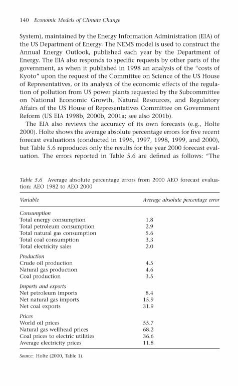
System), maintained by the Energy Information Administration (EIA) ofthe US Department of Energy. The NEMS model is used to construct theAnnual Energy Outlook, published each year by the Department ofEnergy. The EIA also responds to specific requests by other parts of thegovernment, as when it published in 1998 an analysis of the “costs ofKyoto” upon the request of the Committee on Science of the US Houseof Representatives, or its analysis of the economic effects of the regula-tion of pollution from US power plants requested by the Subcommitteeon National Economic Growth, Natural Resources, and RegulatoryAffairs of the US House of Representatives Committee on GovernmentReform (US EIA 1998b, 2000b, 2001a; see also 2001b).

The EIA also reviews the accuracy of its own forecasts (e.g., Holte2000). Holte shows the average absolute percentage errors for five recentforecast evaluations (conducted in 1996, 1997, 1998, 1999, and 2000),but Table 5.6 reproduces only the results for the year 2000 forecast eval-uation. The errors reported in Table 5.6 are defined as follows: “The


Table 5.6 Average absolute percentage errors from 2000 AEO forecast evalua-tion: AEO 1982 to AEO 2000

Variable Average absolute percentage error

ConsumptionTotal energy consumption 1.8Total petroleum consumption 2.9Total natural gas consumption 5.6Total coal consumption 3.3Total electricity sales 2.0

ProductionCrude oil production 4.5Natural gas production 4.6Coal production 3.5

Imports and exportsNet petroleum imports 8.4Net natural gas imports 15.9Net coal exports 31.9

PricesWorld oil prices 55.7Natural gas wellhead prices 68.2Coal prices to electric utilities 36.6Average electricity prices 11.8

Source: Holte (2000, Table 1).

1403_963363_06_cha05.qxd 6/14/2003 11:21 AM Page 140

average absolute forecast error is computed as the mean, or average, ofall the absolute values of the percentage errors, expressed as percentagedifferences of the reference case projection from the actual, shown foreach AEO, for each year in the forecast, for a given variable” (Holte 2000,p. 2). As in the Sanstad et al. study, the quantity forecasts have beenmore accurate than the price forecasts. Keep in mind that these aver-ages cover forecasts made over the entire period from 1982 through2000, and include both short-term (one year ahead, two years ahead,etc.) and longer-term forecasts. Not all of the AEOs contained forecastsreaching as far as 1999 or 2000; the AEOs of 1982–85 did not includeprice forecasts beyond 1995, for example. In addition, the later AEOs’longer-term forecasts cannot be compared to actual prices and quanti-ties, because the actual values after 2000 (the year the analysis was published) could not be known. Thus, these average percentage errorsare weighted towards shorter-term forecasts, which are likely to be moreaccurate than longer-term forecasts. Nevertheless, very large averageerrors in the price projections are evident.

The data presented by Holte also shows that even in the short run,the AEO forecasts contain little or no information about the actualfuture course of energy prices. If the forecasts had any predictive value,a regression of the actual prices as reported by the AEO on the forecastsshould show the forecasts to have some explanatory power. In otherwords, if pf

t,t-i is the forecast of the price of oil (or natural gas) in year tthat was made in year t - i, then a regression of pa

i , the actual price inyear t, on pf

t,t-i should exhibit a significant correlation. Yet for both oiland natural gas, even the forecasts made only one year ahead have noexplanatory power. This is demonstrated by the regression results inTable 5.7. Neither regression provides any evidence for rejecting the nullhypothesis that the forecasts have no predictive power even for the priceonly a year ahead. These results are consistent with the market efficiencynotion that the publicly available forecasts of the EIA can offer tradersno insight into future market developments.

A different methodology to evaluate the accuracy of the EIA’s fore-casts was employed by Shlyakhter et al. (1994). They examined twotypes of energy demand forecasts: a cross-section of 69 energy demandforecasts projected for the year 2000 and projections for approximately180 energy producing or consuming sectors contained in the EIA’sAnnual Energy Outlook.7 Shlyakhter and his coauthors were interestedin comparing the magnitude of actual forecast errors to the reporteduncertainty in the forecasts as measured by the implicit “standard devi-ations” of the forecasts. However, most published forecasts, when they


1403_963363_06_cha05.qxd 6/14/2003 11:21 AM Page 141

report “error bounds” at all, do not express them in terms of a statisti-cally derived standard deviation, because the error bounds arise pri-marily from uncertainties in the assumptions driving the forecasts (suchas the rate of future economic growth) rather than uncertainties in the statistical estimates of model parameters (Shlyakhter et al. 1994, pp. 119–20). To overcome this obstacle, Shlyakhter et al. convert re-ported upper and lower bounds into an estimate of the standard devi-ation of the forecast by making an assumption about the underlyingdistribution characterizing the uncertainty of the forecasts. That is, theyassume that the difference between the upper (U) and lower (L) boundsis k times the implicit standard deviation of the distribution of forecasts(represented by D), or

(5.1)

They then define the “forecast error ratio” x as

(5.2)

where T is the true (realized) value of the variable being forecast and Ris the forecast (the mean or “reference case” of the forecast distribution).If the underlying distribution of the forecasts is normal, it is possible to predict the frequency by which |x| exceeds any particular value. If k = 2 (the value assumed by Shlyakhter et al.), then Pr(|x| > 1) = 0.32,Pr(|x| > 2) = 0.045, etc. (If k > 2, these probabilities would be corres-pondingly smaller.)

Comparison of the actual outcomes to the “reference case” forecastsreveals that the likelihood of large forecast errors is much greater than

x T R k T R U L= -( ) = -( ) -( )D

k U LD = -( )


Table 5.7 Estimated regression equation, pat = a0 + a1pf

t,t-1 + et, 1985–99, world oilprice and natural gas wellhead price from Annual Energy Outlook

â0 â1 R2 Adjusted Regression(Standard (Standard R2 Probability-error) error) Value

Oil 12.241 0.271 0.080 -0.004 0.349(5.746) (0.278)

Natural gas 1.264 0.319 0.103 0.021 0.286(0.607) (0.284)

Source: See text. Data from Holte (2000). Both actual and forecast price variables are innominal terms (dollars per barrel for oil and dollars per thousand cubic feet for gas).There was no AEO 1988 and AEO 1990 did not have a forecast for 1991, so eachregression was based on 13 observations.

1403_963363_06_cha05.qxd 6/14/2003 11:21 AM Page 142

would be predicted if the underlying distribution of forecasts were infact normal. Thus, for the AEO forecasts, the actual likelihood that theforecast error ratio is greater than 1 is approximately 0.7, and the like-lihood that it is greater than 2 is 0.5.8 The same magnitude of forecasterrors (relative to the implicit standard deviation of the forecasts) wasfound for each set of projections – the implicit standard deviations fellas the forecast interval decreased, but the forecast error ratios did not.The performance of the forecasts did not improve when the individualsectors were aggregated, contrary to the authors’ prior expectations(Shlyakhter et al. 1994, p. 123). Their survey of 69 energy forecasts for the year 2000 (a sample distinct from the AEO sectoral sample)showed somewhat lower forecast error ratios, with Pr(|x| > 1) = 0.6 andPr(|x| > 2) = 0.2. These are still substantially larger than if the underly-ing distribution were normal. The likelihood that individual forecastsfall outside a particular distance from the mean is smaller in this casebecause of the much greater diversity of the forecasts (which therebyproduce a larger implicit standard deviation).

What these results mean is that the actual uncertainty underlying theenergy demand forecasts reviewed by Shlyakhter et al. is much largerthan suggested by the forecasts’ “upper” and “lower” bounds. The retrospective analysis by Shlyakhter et al. suggests that the true valueswill be farther from the reference case than the upper or lower boundof the AEO forecast about 70 percent of the time.

5.2.3 Calibration errors in energy-economic models

There certainly is no reason to be confident about the forecasting performance of conventional energy/economic models, based on their record. There is another reason, not commonly recognized, to beskeptical of the models as they are presently constituted. The fuels thatmake up the heart of the energy sector – coal, oil, and natural gas – arecommodities having large stocks relative to their annual consumption.As such, they are “storable” as opposed to “non-storable” commodities(such as perishable fresh fruits or vegetables).9 Williams and Wright(1991) have shown that the array of present and future prices of stor-able commodities is linked by the economic costs and opportunities forstorage, and that any models that fail to take these linkages into accountare bound to give inaccurate and misleading results. Yet the intimateconnection between spot and future prices is absent from the majorforecasting models presently in use.

For example, consider the estimate of the “costs of Kyoto” that wasproduced by the EIA using its NEMS model (US EIA 1998b). The model


1403_963363_06_cha05.qxd 6/14/2003 11:21 AM Page 143

operates in such a way that “[i]n the end-use demand sectors, foresightis assumed not to have a material influence on energy equipment decisions, and such decisions are modeled on the basis of prices in effectat the time of the decision” (US EIA 1998b, p. 20, fn. 22; see also p. 7).Only in the refining and power generation sectors are the producersallowed to exercise foresight, and in the generation sector this foresightis assumed to be perfect in the sense that “[a]n algorithm solves for thepath of carbon prices in which anticipated and realized carbon [permit]prices are approximately the same” (US EIA 1998b, p. 20, fn. 22).

Nevertheless, futures prices are connected to current spot prices andmarket conditions (the level of inventories, anticipated weather condi-tions, etc.); indeed, the spot and futures prices constitute an array of interrelated prices (Williams 1986) that are linked by arbitrage totransportation costs, storage costs, and interest charges. Models such as NEMS are calibrated to yield current prices as the outcome of theirmarket-clearing conditions, but could in principle also be calibrated toincorporate the prices of the various futures contracts that are traded inthe market. If the structure of the models were “correct” (that is, if theyadequately reflected all market and behavioral conditions), the priceforecasts of the models could be accurately linked to futures prices pre-vailing in the current market. After all, these futures prices are tangibleprices just as surely as the spot price of the commodities being traded;ownership of a futures contract gives the holder the legally enforceableright to receive delivery of a specified quantity of a particular com-modity (standardized with respect to grade and quality) at a particulartime and a particular location. The price of such a futures contract isjust as real as the spot price prevailing at any given moment in time.10

Given that future spot prices, current spot prices, and futures pricesare linked, a properly specified model would incorporate all the infor-mation contained in spot and futures prices in its projections of the evolution of commodity prices over time. However, according to theWilliams/Wright analysis, the variance in futures prices declines as theypertain to more distant dates – asymptotically no additional informa-tion is contained in a more distant futures price than what is alreadyincluded in the existing prices. The basic point is that only a limitedamount of information about the future is available to the present.Nothing else is accessible. Even in stylized models in which the struc-ture of the markets, costs of storage, and nature of the intrinsic ran-domness of the economy are explicitly specified, the futures prices canpredict realized prices only with R2 values between 0.1 and 0.3 (Williamsand Wright 1991, pp. 176 ff.).


1403_963363_06_cha05.qxd 6/14/2003 11:21 AM Page 144

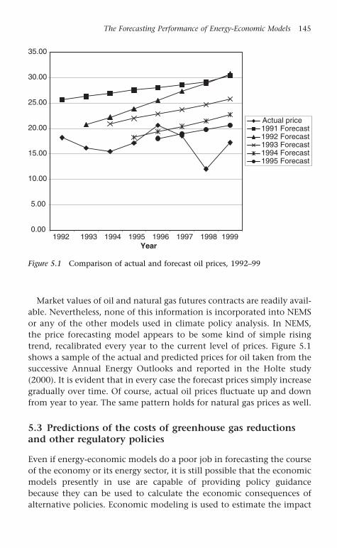
Market values of oil and natural gas futures contracts are readily avail-able. Nevertheless, none of this information is incorporated into NEMSor any of the other models used in climate policy analysis. In NEMS,the price forecasting model appears to be some kind of simple risingtrend, recalibrated every year to the current level of prices. Figure 5.1shows a sample of the actual and predicted prices for oil taken from thesuccessive Annual Energy Outlooks and reported in the Holte study(2000). It is evident that in every case the forecast prices simply increasegradually over time. Of course, actual oil prices fluctuate up and downfrom year to year. The same pattern holds for natural gas prices as well.

5.3 Predictions of the costs of greenhouse gas reductionsand other regulatory policies

Even if energy-economic models do a poor job in forecasting the courseof the economy or its energy sector, it is still possible that the economicmodels presently in use are capable of providing policy guidancebecause they can be used to calculate the economic consequences ofalternative policies. Economic modeling is used to estimate the impact


0.00

5.00

10.00

15.00

20.00

25.00

30.00

35.00

1992 1993 1994 1995 1996 1997 1998 1999Year

Actual price1991 Forecast1992 Forecast1993 Forecast1994 Forecast1995 Forecast

Figure 5.1 Comparison of actual and forecast oil prices, 1992–99

1403_963363_06_cha05.qxd 6/14/2003 11:21 AM Page 145

of changes in taxes, more liberal trade policies, reforms of the criminaljustice system, etc. Instead of trying to cover all these literatures, thefocus here will be on reviewing the performance of contemporarymodels in calculating the effects of regulatory policies (especially of theenvironmental variety).

A recent survey comparing ex ante and ex post cost estimates for regulatory policies found that the studies had a predominant tendencyto overestimate the costs ex ante (Harrington et al. 2000). Harringtonand his coauthors reviewed 28 cases in which ex ante and ex post costestimates were calculated in studies not generated by the regulatedindustries themselves. A forecast was classified as “accurate” if the expost (realized) result fell within the error bounds of the ex ante study orif it varied by no more than ±25 percent from the point estimate of theex ante study. Three categories of forecasts were examined: the quantityof pollution reduction, unit pollution reduction cost, and total cost.Table 5.8 reproduces some of the results of their review. Two main fea-tures of the ex ante/ex post comparison are evident from this table. First,the forecasts are not at all accurate on the whole. Even with the verygenerous definition of “accuracy,” fewer than 30 percent of the forecastswere accurate in predicting either the total cost or the unit cost of theregulations. Second, the tendency of the ex ante studies to overestimateregulatory costs can be seen. This finding is consistent with the earlierstudy by Goodstein (1997), which included industry ex ante estimatesin the comparison set (estimates that Harrington et al. excluded).

There are several notorious examples of the overestimation of regu-latory difficulty or cost in the environmental area.11 Ex ante industryestimates of the per ton cost of SO2 emissions reductions under theClean Air Act Amendments of 1990 were as high as $1500 per ton; theactual cost of the emissions permits as of 2000 were about $200 per ton,


Table 5.8 Case study results on the accuracy of regulatory forecasts

Accurate Overestimate Underestimate Unable to determine

Quantityreduction 13 9 4 2

Unit pollutionreduction cost 8 14 6 0

Total cost 5 15 3 5

Source: Harrington et al. (2000, Table 2, p. 307).

1403_963363_06_cha05.qxd 6/14/2003 11:21 AM Page 146

an increase from $75 per ton in 1997.12 The forecast was off by a factorof 7.5 in this case. Less well known is the case of estimates of the costof eliminating ozone-depleting substances under the Montreal Protocol.Hammitt (1997) found that the actual reductions in CFC-11 and CFC-12 were much greater (given the price increases following the signingof the Protocol) than had been predicted ex ante. Even more dramaticis that the RAND Corporation, in work carried out for the US EPA andpublished in the early 1980s, estimated first that “the most promisingset of mandatory controls could reduce cumulative emissions [of CFCs]over the period [1980–90] by perhaps 15 percent” (Palmer et al. 1980)and then that the available technical options had the potential toreduce CFC emissions by only about one-third (Mooz et al. 1982). It wasthought to be so difficult to find substitutes for CFC-113 as a solvent inelectronics manufacture that there was discussion of excluding it fromthe Montreal Protocol altogether (Benedick 1991). In actuality, CFC pro-duction (except for a few quantitatively unimportant “essential uses”)was phased out entirely in the developed countries by the end of 1996,and will be eliminated in developing countries by 2007. This has beenachieved with no discernable effect on lifestyles or the standard ofliving, and was accomplished in some cases at a net gain to producersand consumers (Cook 1996).

There is no way yet of knowing the impact of mandatory GHG reduc-tions on the US economy, because no regulations have been put in place that would bring about such reductions. However, it is possible tocompare different model estimates of the GDP cost of such reductions.Just such a comparison has been carried out twice in the 1990s by theStanford Energy Modeling Forum. The EMF, in 1993 and 1999, coordi-nated a set of runs, by the leading energy-economic modeling groupsparticipating in the EMF, of comparable emissions reductions scenarios.In the 1993 (EMF-12) comparison, the GDP impact of two alternativecarbon reduction scenarios was simulated, while in the 1999 (EMF-16)runs, the GDP effects of compliance with the emissions reductionstargets of the Kyoto Protocol were calculated under alternative assump-tions about the extent of international allowance trading. The results ofthese comparisons are summarized in Table 5.9. This table shows con-siderable variation in the results from the different models in both EMFexercises, whether measured as the ratio of the maximum estimate ofthe GDP change to the minimum estimate of the GDP change or as thecoefficient of variation of the estimated GDP change.13

In both EMF-12 and EMF-16, the models were run under uniform scenario definitions and the results varied considerably. Yet some of the


1403_963363_06_cha05.qxd 6/14/2003 11:21 AM Page 147

elements of the scenarios are in fact policy options that could be subjectto change. All the EMF scenarios assumed that the tax revenues raisedby a carbon tax sufficient to bring about the requisite CO2 emissionsreductions are returned to the economy as “lump-sum transfers” – aspayments that have no effect on the incentives of producers or con-sumers. However, it is well-known that different methods of “revenuerecycling,” that is, of returning the tax revenues to the economy, havevery different GDP effects (Repetto 2001, Sanstad et al. 2001a).


Table 5.9 Range of estimates of 2010 GDP effects of GHG reduction policies,EMF-12 and EMF-16

Model EMF-12: scenario EMF-16: meeting the Kyoto (% 2010 GDP loss) target (% 2010 GDP loss)

20% No Annex I GlobalStabilization reduction trading trading trading

CRTM 0.2 1.0DGEM 0.6 1.7ERM 0.4 1.1Fossil 2 0.2 1.4Global 2100 0.7 1.5Goulder 0.3 1.2GREEN 0.2 0.9MWC 0.5 1.1

ABARE-GTEM 1.9 0.8 0.2MS-MRT 1.9 0.9 0.3CETA 1.8 0.6 0.4MERGE3 0.9 0.5 0.2RICE 0.9 0.6 0.2AIM 0.4 0.3 0.2G-Cubed 0.4 0.2 0.1

Maximum/ 3.5 1.9 4.8 4.5 4.0minimum

Coefficient of 0.51 0.22 0.57 0.45 0.42variation

Sources: For EMF-12, see IPCC (1996). For EMF-16, see Weyant and Hill (1999) andSanstad et al. (2001a). In EMF-12, the stabilization scenario entails stabilization of CO2

emissions at their 1990 levels by 2000; the 20% reduction scenario means stabilization at1990 levels by 2000 and 20% reduction below 1990 levels by 2010. The EMF-16 estimatedlosses were converted to a percentage of GDP using the forecast of 2010 GDP in IWG(2000), converted to 1990 dollars using the GDP deflator from US Department ofCommerce, Bureau of Economic Analysis (2001).

1403_963363_06_cha05.qxd 6/14/2003 11:21 AM Page 148

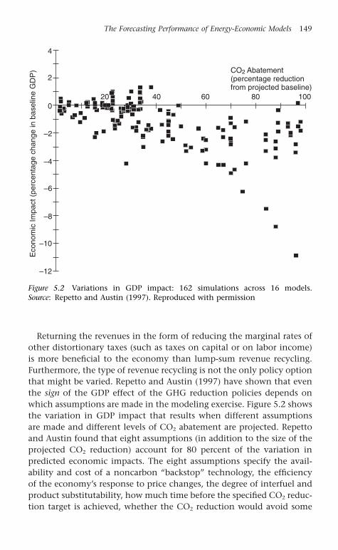
Returning the revenues in the form of reducing the marginal rates ofother distortionary taxes (such as taxes on capital or on labor income)is more beneficial to the economy than lump-sum revenue recycling.Furthermore, the type of revenue recycling is not the only policy optionthat might be varied. Repetto and Austin (1997) have shown that eventhe sign of the GDP effect of the GHG reduction policies depends onwhich assumptions are made in the modeling exercise. Figure 5.2 showsthe variation in GDP impact that results when different assumptions are made and different levels of CO2 abatement are projected. Repettoand Austin found that eight assumptions (in addition to the size of theprojected CO2 reduction) account for 80 percent of the variation in predicted economic impacts. The eight assumptions specify the avail-ability and cost of a noncarbon “backstop” technology, the efficiencyof the economy’s response to price changes, the degree of interfuel andproduct substitutability, how much time before the specified CO2 reduc-tion target is achieved, whether the CO2 reduction would avoid some

The Forecasting Performance of Energy-Economic Models 149E

cono

mic

Impa

ct (

perc

enta

ge c

hang

e in

bas

elin

e G

DP

) CO2 Abatement(percentage reductionfrom projected baseline)

20 40 60 80 100

4

2

0

–2

–4

–6

–8

–10

–12

Figure 5.2 Variations in GDP impact: 162 simulations across 16 models. Source: Repetto and Austin (1997). Reproduced with permission

1403_963363_06_cha05.qxd 6/14/2003 11:21 AM Page 149

of the economic costs of climate change, whether reducing fossil fuelcombustion would avoid other (nonclimate) air pollution damages, and whether “joint implementation” such as international emissionstrading options are available, in addition to how the carbon tax or emissions permit auction revenues are recycled into the economy.

This strong finding that even the sign of the effect of carbon-reducing policies is uncertain has been replicated in subsequent work.Krause et al. (2002) reviewed five major studies generated or relied onby the United States government in addressing the question of the costto the economy of meeting the emissions reductions of the Kyoto Pro-tocol.14 Krause and his collaborators found that while all of the studiesincluded some of the available policy instruments to meet the Kyotoemissions reductions, none of the studies combined all these policies ina least-cost integrated framework. The potential policies included acarbon tax or permit auctions, market and institutional reforms andtechnology programs, tax shifts, international allowance trading, andenhancement of carbon sinks. In addition, none of the analysesincluded the full range of benefits from CO2 emissions reductions, suchas the monetized value of associated local air quality improvements.

The most pessimistic GDP impact estimated was a 4.2 percent loss inthe EIA scenario involving only a domestic carbon tax and no enhance-ment of sinks. (The least pessimistic EIA scenario, which included globaltrading, sinks, and some tax shifting, showed a GDP loss of less than 1percent.) On the other hand, the two “five lab” studies by the Inter-laboratory Working Group showed slight GDP gains, primarily becausethe market reforms and technology policies emphasized in those studies moved the economy towards its production-possibilities frontier(though neither of the five-lab studies achieved the full Kyoto target by2010). The benefit from a least-cost integrated approach to Kyoto isshown in Figure 5.3. Combining international permit trading, tax shifts,and the market, organizational, and institutional reforms outlined inthe five-lab studies results in a net GDP gain of approximately $57billion (1997 dollars) in 2010. The most important component of thisgain is the efficiency enhancement representing movement towards theproduction-possibilities frontier (the market reforms).

These results demonstrate that the outcome of economic analyses ofthe impact of moderate GHG reductions in the United States dependprimarily on modeling assumptions (including definition of the systemboundaries, i.e., whether environmental benefits are included in theanalysis). This robust result underscores the irony of the fact that whilea great deal of attention has been focused on uncertainties in the


1403_963363_06_cha05.qxd 6/14/2003 11:21 AM Page 150

physical science models of the dynamics of global warming, estimatesof the economic impact of various policy responses have been taken atface value. In fact, the uncertainties inherent in the economic analysesare much more serious – as noted above, the physical models are basedon theoretically consistent and experimentally confirmed laws govern-ing physical and chemical processes, while the economic models aregrounded primarily in the assumptions made by the modelers.


It would be going too far to claim that long-run energy/economicmodels have no value just because they have little or no power topredict the course of energy prices and demand. Long-term modelingexercises can be valuable for providing a consistent framework in whichto work out the consequences of various scenarios. This kind of analy-sis is not the same thing as prediction, and the point that should beemphasized is that its primary use should be to explore alternativeassumptions.

At the same time, the poor predictive performance of models of thistype indicates that considerable caution should be used in interpretingthe results of model runs. If technological change is the main driver ofeconomic change over the long run, it would be unwise to place toomuch faith in models that represent technological change in only themost stylized fashion (Sanstad 2000). If not only the magnitude, buteven the sign of the effect of a proposed policy depends on contestable


–10

0

10

20

30

40

50

60

70

Internationalpermits

Substitutionlosses

Tax shiftoffsets

Environmentalco-benefits

Marketreforms

Net economicimpact

Sav

ings

rel

ativ

e to

ref

eren

ce c

ase

($'9

7 bi

llion

/yr)

Figure 5.3 US cost and savings components of a least-cost Kyoto strategy withglobal trading, 2010. Source: Krause et al. (2001)

1403_963363_06_cha05.qxd 6/14/2003 11:21 AM Page 151

model assumptions, then the results of the analysis need to be takenwith a very large grain of salt. Energy modeling in economics has a longenough history that the match between forecasts and actual outcomescan be compared. The result of such comparisons is not encouraging forthose who would invest economics with an aura of scientific precision.This does not mean that economists should abandon the effort to gaininsight into the forces shaping the long run; it only means that theymust be conscious of the limits to their ability to do so.


1403_963363_06_cha05.qxd 6/14/2003 11:21 AM Page 152

6Principles for the Future

153

The previous chapters have shown that by downplaying or ignoring theissues of distribution, multiple equilibria, and dynamics, the economicanalysis of climate policy has missed (or mischaracterized) essentialaspects of the problem. Most analysis has concentrated on matters ofefficiency that are more suitable for small-scale environmental problems(such as where to locate a landfill or what to do about pollution of ariver by an industrial plant) than for a global issue like climate change.By implicitly taking the existing definitions and distribution of prop-erty rights for granted, policy advice has been skewed towards the statusquo. Some of the possibilities that are opened up by the creation ofclimate rights or alternative evolutionary paths for the economy havebeen ruled out arbitrarily, when they may actually offer the mosthopeful potential routes to climate stabilization.

The result of this modeling failure has been a bias against bold andtimely action, overestimation of the cost of emissions reductions, andpervasive paralysis in the political debate. By treating technology as aconstraint on production, rather than as a dynamic process of innova-tion, the consequences of climate policy initiatives have been seenalmost entirely in terms of adverse trade-offs. By ignoring the wealtheffects associated with the creation of new climate rights (and from thedestructive consequences of large-scale climatic disruptions), the welfareanalysis of climate change has been couched almost exclusively in termsof changes in ordinary GDP (sometimes with climate damages “mon-etized” at current prices). This means that the “costs” of climate changehave been estimated as marginal displacements of consumption or GDP.The strong negative impact of the risk of climate disruption has beensystematically downplayed. No attention has been given to the poten-tial constituencies who would favor climate policy activism.

1403_963363_07_cha06.qxd 6/14/2003 11:22 AM Page 153

Nothing has been more destructive of progress and consensus in thearena of international climate diplomacy than the focus on efficiencyto the exclusion of equity concerns. The United States in particular,throughout the Kyoto negotiations and up to the very end of our mean-ingful participation when the Bush Administration repudiated thetreaty, clung obsessively to the need for “flexibility mechanisms” suchas international trading of emissions rights as a precondition for ourinvolvement. The reason was a determination to lower the purportedcosts of the policies through purchase of Russian “hot air,”1 takingadvantage of low-cost emissions reduction opportunities in developingcountries, and counting enhanced carbon sinks as part of the nationalemissions reductions. US government analyses consistently placed greatstore in the cost-reducing possibilities of international trading of emis-sions rights, even though more comprehensive calculations show thata determined domestic emissions reduction strategy could achieve theKyoto target at no net loss to the economy (Krause et al. 2002).

Of course, attempting to negotiate the devilish details of the flexibil-ity mechanisms created a nightmare of complexity. Questions of re-porting, compliance, and enforcement loomed large. As the developedcountry representatives attempted to work out an acceptable set of rules,the developing countries remained largely outside the process. Thedeveloping countries were determined to address the equity issuesinvolved in setting current and future emissions targets. They alsowanted to guarantee the kinds of technology transfers and capital flowsthat would forestall any conflict between climate protection and theirown economic growth.2 While the United States, driven by its insistenceon economic efficiency, demanded international permit trading regard-less of what the emissions targets might be, the developing countriesfocused on how to rectify the large historical discrepancies in cumula-tive emissions resulting from the fact sustained economic growth hadbegun much earlier in the developed countries. “Meaningful participa-tion by developing countries” in a Kyoto-like emissions reductionscheme was thus subject to conflicting interpretations: the rich coun-tries rightly saw that without full global participation, any climate protection program was ultimately doomed to fail over the long run. In opposition, the developing countries feared institutionalization ofsomething like current emissions levels (or ratios) that would condemnthem to permanent economic inferiority because of the advantages therich countries had derived from their historic reliance on fossil fuels topower the industrial revolution.


1403_963363_07_cha06.qxd 6/14/2003 11:22 AM Page 154

The preoccupation with efficiency by the United States was anexample of the bias created by taking existing definitions of propertyrights for granted. Ignoring the wealth creation and destruction thatmust accompany any meaningful change in the pattern and cost offossil fuel use (or perhaps more accurately, addressing the distributionalissues only indirectly rather than openly and transparently), the USposition sowed seeds of suspicion and distrust that plagued the negoti-ations from the start. A per capita based assignment of property rightsin carbon emissions would have immediately created a powerful con-stituency for a climate protection regime in the developing countries,because their populations would have received the largest share of thecarbon rights. If such an equity foundation had been laid, the rich coun-tries would have faced cooperation rather than opposition from thedeveloping world, and would have been free to move ahead in thedesign of efficient market mechanisms based on a distribution of carbonrights that would command support of the poorer countries. Such anassignment of climate rights would entail a substantial transfer ofwealth from the developed to the developing world, but it is entirelypossible that the citizens of the rich countries would be willing to acceptsuch a transfer (and the accompanying changes in their energy use pat-terns) if they felt that the policies were actually going to be effective insolving the climate and development problems over the long run.3

Kyoto did not resolve these tensions. Although the emissions reduc-tions called for by the treaty were significant (for the United States, 7percent below 1990 levels as of 2008–12 would have amounted toroughly a 30 percent reduction in emissions from the business-as-usualbaseline), they are far short of what will be required to avoid “danger-ous anthropogenic interference with the climate system” (the phrasefrom the text of the 1992 United Nations Framework Convention onClimate Change).4 Yet even Kyoto’s first steps could not be achievedwithout significant policy initiatives including a carbon tax or emissionspermit system. While the setting of emissions standards through inter-national negotiations could be interpreted as a partial “loss of sover-eignty,” the new property rights implicitly created by such a processcould be part of a larger consensus solution to the climate problem.Rather than seeking short-term national advantage in lawyerly fashion,the United States could have taken the lead to reach international agree-ment based on the creation of new climate rights.

It should have been acknowledged from the outset that the creationof these rights would have a significant (but not overwhelming) effect

Principles for the Future 155

1403_963363_07_cha06.qxd 6/14/2003 11:22 AM Page 155

on personal and national wealth. The redistribution would not neces-sarily have a permanent effect on any nation’s or region’s prosperity,however. If there is sufficient intergenerational economic and socialmobility, the consequences of any initial distribution of property die out over time through the normal working of the market process. Thevoluntary market exchanges that take place in a dynamic economyguarantee that the future pattern of wealth ownership is almost entirelyindependent of the initial distribution (DeCanio 1992). The proper roleof the market is to decentralize decision-making as much as possiblegiven a suitable definition of property rights. When a new problem suchas anthropogenic climate change develops, it is appropriate to extendthe scope of property rights to bring the externality under control. Effi-ciency gains realized through markets then have an important role inmaintaining economic growth and vitality. However, it is a distortionof the virtues of the market economy to argue that a status quo basedon an incomplete set of property rights is somehow “optimal” or that toprotect the environment necessarily involves economic losses.

It is also the case that creation of new climate rights would enablethe political process to “manage inequality” in a relatively benignfashion. Redistribution can turn ugly, especially when currently definedrights are taken away from some and given to others in a coercive zero-sum fashion. In contrast, the creation of new rights offers the opportu-nity to associate the inevitable redistributions with a higher socialpurpose – in this case stabilization of the climate. The climate problemhas to be solved if humanity is to survive in the long run; it is also thecase that sustainable development and the elimination of mass povertyare required if the future is to be stable and peaceful. Either of thesetwin necessities would in itself justify a fresh look at property rightsassignments.5 An intelligent policy of climate rights creation couldaddress both problems at once.6 In any event, it is futile to adhere tothe fiction that doing nothing is the conservative course – inactionredistributes rights as surely as conscious action, as the damages ofclimate change and risks of climate catastrophe make themselves felt.

The preceding chapters have shown how assignment of climate rightsaffects all aspects of the economic system, including interest rates. If weare to avoid the moral arrogance of selecting the present as the preferredtemporal vantage point, it is also clear from the simple models workedout earlier that some kind of ethical system balancing the benefits andobligations of different generations is required. Neither the marketsystem nor democratic majoritarianism offers a ready-made solution.Rules based on deeper notions of intergenerational justice are necessary.


1403_963363_07_cha06.qxd 6/14/2003 11:22 AM Page 156

The development of such principles is the subject of a different study,although it seems plausible that ideas such as the Golden Rule wouldoccupy a central place in such an endeavor.7

In much the same way that equity and efficiency cannot be disen-tangled, so it is with economic dynamics and the progress of tech-nology. We have seen that neither the modern theory of the firm, theevidence on intra-industry heterogeneity, nor the logic of evolutionarymodels supports the representation of production by the “profit maxi-mization subject to a production function” model. Standard generalequilibrium models do not embed a coherent dynamic story, so takingdynamics as the starting point for the modeling of production wouldresult in no loss of information but would have the potential for sig-nificant gains in realism.

An important consequence of the results developed in the previouschapters is that claims to be able to estimate precisely the “costs” ofclimate protection policies must be abandoned. If firms are not on awell-defined production-possibilities frontier, and if the dynamics oftechnological progress are only imperfectly understood, then any hopeof exact calculation of the costs of alternative policies vanishes. Un-conventional policies, such as voluntary pollution-reduction programs,government–industry partnerships, and internally generated corporate“greening” campaigns can be effective. At the same time, the effects ofa carbon emissions price increase – substitution in favor of less carbon-intensive products, the accelerated development of energy-efficiencytechnologies, and the promotion of market and institutional reformsthat improve productivity in multiple dimensions – cannot easily bedisentangled.

A corollary is that it is fruitless to attempt to determine the “optimal”carbon tax. If neither the costs nor the benefits can be known with anyprecision, just about the only thing that can be said with certainty aboutthe welfare-maximizing price of carbon emissions is that it is greaterthan zero. Economists have a great deal to say about how to implementsuch a tax efficiently and effectively, about the similarities and differ-ences between a tax and a system of tradable carbon emissions permits,and about the best way to recycle the revenue from such a tax or permitsystem. And, as we have seen above, the distributional consequences ofsuch a tax or permit auction plan will affect other economic variablesthrough system-wide feedbacks. However, any attempt to specify theexact level of the “optimal” tax is less an exercise in scientific calcula-tion than a manifestation of the analyst’s willingness to step beyondthe limits of established economic knowledge.


1403_963363_07_cha06.qxd 6/14/2003 11:22 AM Page 157

Despite the limitations of their models, economists have been willingto play a central role in the policy discussion, and there is no doubt thatthey have had a great deal of influence on the debate. Power is seduc-tive; susceptibility to its attractions is not evidence that economists asa group are more self-promoting or venal than natural scientists or othersocial scientists.8 Instead, the failure of economics derives from a kindof hubris on the part of the profession. The technical achievements ofeconomics, particularly of mathematical general equilibrium theory,have engendered an attitude of superiority vis-à-vis other disciplines.More seriously, the limitations and unanswered questions that lie at theheart of general equilibrium theory have been ignored in the drive toprovide answers that can carry political weight.

In fairness, it is difficult to imagine what a true social science wouldlook like if it were not based on some simple unifying principles. Thedanger, however, is in settling on abstractions that leave out essentialfeatures of the social process. By reducing human behavior to axiomat-ically defined rationality and maximization, it is possible to confuse realeconomic problems with purely mathematical ones. Models can alwaysbe set up in such a way as to be analytically tractable, whether or not mathematical convenience is a feature of the economic reality themodels are intended to represent. The ability to solve mathematicalpuzzles, while requiring a great deal of ingenuity and high-poweredintellectual skills, conveys a sense of power and accomplishment thatis easily mistaken for real wisdom. Thus, economists can slip into themode of offering advice and policy prescriptions on the basis of theresults of their models, even though the models do not adequatelycapture the key features of the social world.

It is perhaps understandable that economists desire to emulate thenatural scientists by seeking sparse and elegant mathematical descrip-tions of the social system. Unfortunately, this quest has so far provento be futile. As discussed in the previous chapters, it has been knownfor some time within economics that the most parsimonious repre-sentations of rationality do not provide sufficient restrictions on the behavior of aggregates of diverse individuals to determine a uniqueequilibrium. There are limits on what economics can say, given onlythe requirements of formal rationality. By disregarding these limits incarrying out climate policy analysis based on neoclassical general equi-librium theory, economists have constructed an imposing structure onunsound foundations. While the edifice has the trappings and appear-ance of scientific rigor, its “results” are in fact derived in large part fromunverified or untrue assumptions.


1403_963363_07_cha06.qxd 6/14/2003 11:22 AM Page 158

Despite its limitations, economics can make an important contribu-tion to the formation and implementation of a climate policy that treatsall people and all generations fairly. Just because general equilibriummodels cannot provide the kind of precise guidance that politicianswish for, it does not follow that economics appropriately conceived isdevoid of useful insights. Before Kyoto, at least, there was actually quitea high degree of consensus about climate policy among a wide range ofeconomists. The Economists’ Statement on Climate Change of early1997 reflected this consensus – it called for action on the problem, inter-national cooperation, and use of market mechanisms to implement reg-ulatory action. It noted that responsible policies would not harm theUS standard of living and might even “improve US productivity in thelonger run.”9 Economists understand the power of compound growth,and realize that even if policies to reduce GHG emissions reductionswere to reduce GDP by 1 percent below a business-as-usual baseline permanently, this would only cause a delay of approximately sixmonths in achieving any given level of per capita income (based on the economy’s historical annual real per capita growth rate of around 2 percent).

The advice offered by the Economists’ Statement on Climate Changeis quite broad and vague as to specifics. Practical policies have to bemore explicit about just what carbon tax rate would be enacted, exactlywhat would be done with the revenues, how much and what kinds ofR&D would be subsidized, and so forth. Economists have much to sayabout such issues. There should be nothing surprising about this – eco-nomics began as “political economy,” after all, and part of its purposealways has been to inform policy. And because so much of what passesfor “economic policy” generated by politicians and special interestgroups is so stupid and misguided, economists have good reason to feelsuperior. (Think about rent controls, protectionist trade barriers, andpoorly drawn regulations.)10

These considerations do not give economists carte blanche to saywhat should or should not be done to protect the global environment,however. Some of the models being used for climate policy work evolvedfrom the energy/economic models developed in the 1970s in responseto the oil price shocks. It is not at all clear that the framework appro-priate for analyzing the earlier problem is well-suited for the current situation. The climate problem hinges on issues that are very poorlyhandled by conventional energy economics – matters of distributionalequity, nonmarket environmental quality, intergenerational fairness,and the internal workings of firms. Instead of relying on flawed general


1403_963363_07_cha06.qxd 6/14/2003 11:22 AM Page 159

equilibrium models to point the way, we could start from a specifica-tion of the characteristics of the future (or potential futures) we wish tobequeath to our successors and work backwards.11 Economics has muchto contribute to policies that can bring about a desirable future. Fromthe arithmetic identity that points to the need for decarbonization (andmore generally, dematerialization) of production12 to the design of in-centives that actually can bring about intended outcomes, economicknowledge and insight should be an integral part of the policy process.

At the most fundamental level, however, while economics can offerinsight it does not provide solutions. An ethical foundation for climatepolicy must be established that recognizes the rights and obligations ofall generations. This foundation has to recognize that not all affectedparties are able to participate in either the market or the politicalprocess. A majority of those whose lives will be affected by the futureclimate are disfranchised because they do not yet exist. They possess nopresent-day economic power, and have no way of expressing their pref-erences in a tangible way. The only way to protect persons living in thefuture is through some kind of Intergenerational Constitution thatspells out their rights, a Constitution that the present generation is com-mitted to abiding by. Of course, it is always possible that we who arealive today will forsake our duty, and will make choices reflecting anattitude of domination over the world and the future rather than a senseof stewardship. The present generation always has the power to disre-gard the well-being of future generations or, for that matter, those whoare powerless in the present day. This kind of power is an intrinsicelement of human freedom, and the potential for its misuse is part ofthe tragedy of the human condition. Nevertheless, we have a responsi-bility to use our power wisely, in the hope that those who follow us willremember us with affection and honor rather than with an astonisheddismay at our folly.


1403_963363_07_cha06.qxd 6/14/2003 11:22 AM Page 160

Notes

161

1 An Overview of the Issues

1. The IPCC was jointly established in 1988 by the World Meteorological Organization (WMO) and the United Nations Environment Programme(UNEP). It draws on the work of hundreds of experts from all regions of theworld in presenting reports to the parties engaged in negotiations under theUnited Nations Framework Convention on Climate Change (UNFCCC), andrepresents the mainstream scientific consensus (or range of opinion wherethere is no consensus) on climate issues. The IPCC has produced to datethree Assessment Reports (1990, 1995, and 2001) covering all aspects ofclimate change.

2. In the terminology of Working Group I of the IPCC, “very high confidence”means having a probability of 95 percent or more.

3. It should be noted that the statement in the preceding quotation thatclimate change will affect human welfare “positively and negatively” is basedon the findings of some studies estimating that segments of the popu-lations of certain countries might benefit from limited climate change.

4. Partial equilibrium analysis usually involves examination of only one marketin isolation. The supply and demand curves of introductory economicscourses are the icons of this approach.

5. Examples of climate policies analyzed include measures such as a tax oncarbon emissions, a system of tradable emissions permits, or incentives topromote technical change to increase energy efficiency.

6. A fine historical overview is given by Ingrao and Israel (1990).7. It is an open philosophical question why mathematical models work so well

in the physical sciences. It can be argued that mathematics somehow corre-sponds to the nature of physical reality, or that logical thought evolved inconformity with physical reality because such thinking would have survivalvalue. However, this view just pushes the question back a level – why shouldwhat has survival value to creatures operating on human-sized scales haveapplicability to the motions of planets and stars, or to the structure of in-visible realms at the atomic level that can only indirectly be perceived byhumans? It is clear that the current frontiers of physics – the paradoxes ofquantum theory, the higher dimensions of string theory, and the outlinesof alternative grand unification schemes – are so far from our ordinary expe-rience that the concepts can only be formulated in abstract mathematicalterms. For a classic discussion of the mystery of the effectiveness of mathe-matics in explaining physical phenomena, see Wigner (1960). As he puts it,“[t]he miracle of the appropriateness of the language of mathematics for theformulation of the laws of physics is a wonderful gift which we neitherunderstand nor deserve. We should be grateful for it and hope that it willremain valid in future research and that it will extend, for better or for worse,

1403_963363_08_note.qxd 6/14/2003 11:25 AM Page 161

to our pleasure, even though perhaps also to our bafflement, to widebranches of learning.” It has also been suggested that the success of mathematics in the natural sciences is partly the result of focusing only on those phenomena that can be described using traditional mathematicalmethods (see Wolfram 2002).

8. As Krugman says,

academic economics . . . [is] a primitive science, of course. If you want aparallel, think of medicine at the turn of the [19th] century. Medicalresearchers had, by that time, accumulated a great deal of informationabout the human body and its workings, and were capable of giving somecritically useful advice about how to avoid disease. They could not,however, cure very much. Indeed, the doctor/essayist Lewis Thomas tellsus that the most important lesson from medical research up to that timehad been to leave diseases alone – to stop the traditional “cures,” likebleeding, that actually hurt the patients. (1995, p. 9)

9. Strictly speaking, an “integrated assessment” model would have fully de-veloped atmospheric, geophysical, and biological components coupled tosocioeconomic components tracking population, emissions, and policy vari-ables. In actuality, the general equilibrium models used for policy analysisare almost exclusively economic models, with the climate components in-cluded in only the most stylized way (through a “damage function” basedon average surface temperature, for example). The term “integrated assess-ment” will be used to describe the models treated in this book, with theunderstanding that what is being discussed is the economic modeling andnot the physical science side.

10. A “Pareto optimum” is an allocation of goods and services such that no indi-vidual’s material situation (or welfare) can be improved without worseningthe situation of at least one other person. Movements towards a Paretooptimum can, at least in principle, command social unanimity; movementsaway from a Pareto optimum cannot.

11. The modeling philosophy that will be carried throughout the followingchapters is that the value of models is to illustrate arguments clearly andsharply. The models are not intended to be “descriptive” or all-inclusive.Indeed, one of the points that will be made again and again is that fullydescriptive modeling is beyond the capacity of economics at the presenttime. There is also a difference between using models to claim to describewhat does happen and using them to show what might happen. The formeris the style of much current applied economics, including the general equi-librium climate policy models. The latter is what will be pursued in this book.

12. An interesting current example has to do with the nature of the Social Secu-rity entitlement. The Social Security Trust Fund has purchased trillions ofdollars worth of US Treasury securities during the years it has been runninga surplus. These purchases have enabled the federal government to havehigher expenditures and lower taxes that would have been possible if theSocial Security Administration had not been buying the Treasury bonds. Atsome point in the future, however, annual payroll tax receipts will no longerexceed Social Security payouts, and the Social Security system will have to

162 Notes

1403_963363_08_note.qxd 6/14/2003 11:25 AM Page 162

draw on first the interest, then the principal, of its Treasury bond holdingsto meet the Social Security entitlements. The government could, of course,repudiate the bonds and declare that the entitlement was reduced. Thismight be politically very difficult, and it might fairly be described as im-moral, but it is possible because of the sovereignty of the State.

2 The Representation of Consumers’ Preferences andMarket Demand

1. Competitive behavior also may diverge from economic rationality. A partic-ularly striking example of this is the “Dollar Auction Game” first describedby Martin Shubik (1971) and elaborated by Mérö (1998). In this game, adollar is auctioned to the highest bidder, with the proviso that the second-highest bidder must also pay the auctioneer the amount that he bid. In bothcasual and formal experimental settings, the “winning” bid is typically con-siderably higher than $1.00. Shubik reported that in social settings, theaverage paid for the dollar was $3.40. Competitiveness, emotion, and a desirenot to be made a fool of drive the bids considerably above the “economic”value of the dollar.

2. Ethical questions aside, Lane (2001) brings together research from a numberof fields to make the case that once people are above the poverty level, ad-ditional income has little to do with happiness and that friendship and agood family life are the main sources of well-being in advanced economies.It is well-established that average reported levels of subjective happiness ina given country do not change very much as aggregate per capita incomegrows over time, although subjective happiness scores are positively re-lated to income at a given point in time. See the survey by Frey and Stutzer(2002).

3. Indeed, this feature, coupled with the empirically testable notion that amarket system free of discrimination will eventually lead to a distribution ofwealth independent of the “initial conditions” (even an unjust “original”wealth distribution based on conquest), is the strongest argument for thejustice of the market system. See DeCanio (1992) for a full discussion.

4. In particular, environmental externalities can be seen as arising from a lackof property rights, or from the difficulty of their enforcement due to hightransactions costs. See Coase (1960), Dahlman (1979), Macaulay and Yandle(1977), and Dales (1968).

5. The idea that emissions rights should inhere primarily in the population asa whole has even been embodied in proposed legislation: the Clean PowerAct that would reduce emissions of four major power plant pollutants includ-ing CO2. The Clean Power Act as of June 2002 had 22 Senate and 128 Housecosponsors (NRDC 2002).

6. To read an encompassing critique of CBA as it is currently practiced, see Heinzerling and Ackerman (2002).

7. Some economists have attempted to develop a theory of “rational ad-diction” to explain widespread destructive phenomena such as cigarettesmoking and illegal drug use (e.g., Becker and Murphy 1988, Dockner and

Notes 163

1403_963363_08_note.qxd 6/14/2003 11:25 AM Page 163

Feichtinger 1993). Needless to say, this theory relies on a highly contestableconcept of “rationality.”

8. It is interesting that smokers on average have an unrealistically high estimateof their odds of dying from the effects of smoking (Viscusi 1991).

9. See Haddad and Howarth (forthcoming) and Diamond and Hausman (1994)for a full discussion of these and other conceptual and empirical flaws in theCV methodology. Needless to say, the validity of the CV methodology ishotly disputed. In addition to the Diamond and Hausman paper, the sym-posium on Contingent Valuation in the Autumn 1994 issue of the Journal ofEconomic Perspectives contains a spirited defense of CV by Hanemann (1994)and an overview by Portney (1994). In a recent contribution, Carson et al.(2001) conclude that “many of the alleged problems with CV can be resolved by careful study design and implementation” and that “claims that empirical CV findings are theoretically inconsistent are not generallysupported by the literature” (p. 173). Consensus within economics on thevalidity and limits of CV has yet to be reached.

10. Obviously, the political rules matter. Some revenue-raising measures mayrequire a supermajority (such as a two-thirds or three-fourths majority), andsome property rights may be relatively inviolable on constitutional grounds.

11. Efforts to impose the rational maximization paradigm in nonmarket areas,such as the “economics of marriage and the family,” the “economics ofcrime” (as well as the “economics of rational addiction”) overreach and tendto confuse the fact that people respond to incentives with a full explanationof behavior. The two are quite different.

12. As Popper showed many years ago, statements that are tautologically trueand therefore immune to empirical testing cannot constitute the foundationof any science; truly scientific propositions must at least in principle be fal-sifiable (Popper 1968 [1934]).

13. This situation may be changing. Economists have begun to draw on andcontribute to the extensive literature that deals scientifically with humanactions that do not fit the strict definition of economic rationality. SeeLaitner et al. (2000) and the references cited therein, or the session of the2000 Annual Meeting of the American Economic Association titled “Prefer-ences, Behavior, and Welfare” that had papers devoted to “Emotions in Economic Theory and Economic Behavior” (Loewenstein 2000) and also“Thinking and Feeling” (Romer 2000). The National Bureau of EconomicResearch currently has a Working Group on Behavioral Finance (NBER 2002).The 2002 Nobel prize in economics was awarded in part for work in behavioral economics. Whether or not this approach will find its way intointegrated assessment modeling remains to be seen.

14. There have been some interesting efforts to derive the weakest set of conditions on individual utility functions or the distribution of individualcharacteristics that would imply well-behaved aggregate demand functions.See, for example, Hildenbrand (1994), Härdle et al. (1991), Freixas and Mas-Colell (1987), and Jerison (1982). This important work has had essentiallyzero impact on the practice of integrated assessment climate modeling. As will be shown below, the empirical studies on the way environmentalgoods enter individuals’ preferences that would need to be done to bring tobear on climate models the insights of the theorists remain undone, and

164 Notes

1403_963363_08_note.qxd 6/14/2003 11:25 AM Page 164

may be impossible to carry out in the absence of property rights and marketsin the key environmental goods.

15. There is a correspondence between the axiomatic and utility function ap-proaches, with major points of overlap and some minor technical differ-ences. A detailed treatment is given by Mas-Colell et al. (1995).

16. See Ackerman (1998), Laitner et al. (2000), or Mas-Colell et al. (1995). Ingraoand Israel (1990) place the development of these ideas in the context of thehistory of economic (and scientific) thought on the subject of equilibrium.The result that aggregate market demand curves can have virtually any shapeis usually referred to as the Sonnenschein–Mantel–Debreu theorem after thetheorists who wrote the pioneering papers.

17. Here is an indicative example: the handbook Applying General Equilibrium(Shoven and Whalley 1998 [1992]), in the respected Cambridge Surveys ofEconomic Literature series, makes no mention of “uniqueness” or “stabil-ity” in its index. The authors do allude to the fact that some numericalmethods for solving the systems of equations have convergence problems(pp. 41–2), and they acknowledge that “[t]here are no guarantees that suchprocedures [price adjustment processes in which prices are raised for com-modities with positive excess demands and lowered for commodities withexcess supplies] will converge because the excess demand functions mayhave local inflection points, changes in slope, or both . . . whence our needfor a more elaborate computational method of finding counterfactual equi-libria” (p. 39). Whether or not “a more elaborate computational method offinding . . . equilibria” has any correspondence to economic reality is notexamined. This point will be developed in the following section.

18. Analogous results can be obtained in models with production. Indeed, thepossibilities for multiple equilibria in economies with production may begreater than in exchange economies. Timothy Kehoe (1985) says,

Unfortunately, the conditions required for uniqueness of equilibrium inproduction economies appear to be more restrictive than those in pureexchange economies. For example, it is well-known that, if either theweak axiom of revealed preference or gross substitutability is satisfied bythe consumer [aggregate] excess demand function, then a pure exchangeeconomy has a unique equilibrium. This is not the case for an economywith production. (pp. 120–1)

Aside from their simplicity, there is an additional reason to restrict our attention to exchange models rather than models involving production.Intertemporal models with production typically focus on the choice betweensaving and consumption. However, this makes the choices and opportuni-ties of future generations contingent on the savings/consumption decisionsof the present generation, because the capital available to the future gener-ations will depend on how much saving is undertaken by the present gen-eration. If the analysis means to treat the generations in an ethically neutralfashion (with no generation having an analytically preferred vantage point),the endowments of each generation should be in some sense independentof the choices and preferences of the others. This condition is most easilyrepresented in exchange models. Intertemporal models of this type will be

Notes 165

1403_963363_08_note.qxd 6/14/2003 11:25 AM Page 165

developed more fully in Chapter 3. It should be noted that generalizationsof these ethically neutral exchange models are possible if the endowmentschange over time exogenously, as is the case if “autonomous” technicalprogress is providing the impetus for economic growth.

19. If the benefit/cost ratio differs from one at the imputed price of the en-vironmental goods, then the economy cannot be in equilibrium; the envi-ronmental policy has to be implemented until the ratios of marginal utilityto price are equalized across all goods (including the environmental goods).

20. The setup of this model economy will follow the example given by Kehoe(1998). Kehoe illustrated multiple equilibria in an exchange economy withonly two agents and two goods; the examples developed subsequently in thetext are straightforward generalizations.

21. Obviously, there is nothing intrinsic about this assumption of an equalnumber of agents and goods. It is adopted purely for expositional con-venience.

22. It should be noted that in the real economy, not only do different pairs (or combinations) of goods have different degrees of substitutability, butthose elasticities of substitution may change over time. The degree of sub-stitutability between goods may also differ with the consumer’s income level.

23. In the limit as bi Æ 0, the utility function of equation (2.1) becomes ui = Sjaij log(xij). This can be seen by subtracting one from the numerator ofeach of the summed terms in equation (2.1) (a monotonic transformation of a utility function yields an equivalent utility function) and applying L’Hospital’s rule to calculate the limit. In the Cobb–Douglas utility function(ui = Pjxij

aij), the elasticity of substitution between goods is one; in the Leontiefutility function (ui = min[(xi1/bi1), (xi2/bi2), . . . , (xin/bin)]), the elasticities of sub-stitution are zero. Note that ui = Sjaij log(xij) is the same as Cobb–Douglas utility,because the two utility functions differ only by a monotonic transformation(in this case, taking logarithms of the Cobb–Douglas function).

24. Substitutes and complements can also be defined in terms of the responseof the demand for one good to a change in the price of the other. That is,if the demand function for (say) the first good is given by h(p1, p2), then thetwo goods are complements (at a particular pair of values of the prices) if∂h(p1, p2)/∂p2 < 0; they are substitutes if ∂h(p1, p2)/∂p2 > 0. The partial deriv-ative ∂h(p1, p2)/∂p2 can be converted into an elasticity by multiplying byp2/h(p1, p2), and the resulting “cross-elasticity of demand” will have the samesign as the partial derivative. To simplify both the mathematics and theexposition, the models used in the text will be of the constant elasticity ofsubstitution type, so that the degree of substitutability of the commoditiesdepends exclusively on the bi parameters as in equation (2.3).

25. This normalization rule is adopted to facilitate the numerical search for equi-libria. With the prices restricted to lie between zero and one, the startingpoints for the numerical search for equilibria can be confined to a well-defined region. The substantive results are the same if a numeraire good isselected and its price is set equal to one, because the relative prices are thesame in either case.

26. The general equilibrium system was solved numerically in Mathematica(Wolfram 1999).

166 Notes

1403_963363_08_note.qxd 6/14/2003 11:25 AM Page 166

27. For this exchange economy, GDP is Sjpj(Sixij) = Sjpj(Siwij). The constancy of GDP follows from the symmetry of the endowments (so that Siwij isthe same for all j) and the fact that the prices are normalized to sum to one.

28. Note that with five agents, the Gini for the most extreme degree of inequal-ity (all the income accruing to a single agent) is 0.8.

29. The fact that the equilibria of a competitive market economy are Paretooptima is just the first fundamental welfare theorem. As noted earlier, itrequires an absence of externalities, perfect information, no collusion, andthe other standard assumptions of the competitive general equilibriummodel.

30. This is essentially the same as the instability of prototypical zero-sum gameof “Couples” discussed by Riker and Ordeshook (1973). In real politics, otherpreferences not reflected in the model may determine which majority coali-tion actually is formed.

31. Kehoe (1998) shows how the index theorem can be used to derive necessaryand sufficient conditions for the uniqueness. See also note 39.

32. In this case Newton’s method exhibited convergence problems from somestarting points. It is possible that there are more equilibria in this economy,but for many different initial price vectors Newton’s method did not con-verge, even after thousands of iterations.

33. For purely mathematical reasons, the number of equilibria must always beodd. See Dierker (1972).

34. In particular, Mathematica’s FindRoot procedure was used with differentstarting points. In this application (in which formulas for the derivatives of the equations being solved simultaneously can be calculated explicitly),FindRoot uses Newton’s method or the secant method (Wolfram 1999, pp. 919–22).

35. Exceptions, such as the Goulder–Schneider model (1999), rely on ad hocadjustment processes that are akin to the tâtonnement that will be describedpresently.

36. Considerable effort from the time of Walras and Marshall onward (see Ingraoand Israel 1990) has been expended to develop dynamic theories that areconsistent with the equilibrium model. Despite all the good work that hasbeen done, Fisher’s assessment (1989) indicates how much remains: “[W]ehave no rigorous basis for believing that equilibria can be achieved or main-tained if disturbed. . . . [T]here is no disguising the fact that this is a majorlacuna in economic analysis” (p. 36), and “[N]ew modes of analysis areneeded if equilibrium economic theory is to have a satisfactory foundation”(p. 42).

37. According to Hahn (1989), the Walrasian “auctioneer” calls out hypotheticalprices in one market at a time and adjusts them according to the excessdemand. When equilibrium is reached in one market, the auctioneer moveson to the next market. Interestingly, Fisher, in the same New Palgrave volume(1989), states that “[t]he question of who adjusts prices . . . is typically leftunanswered or put aside with a reference to a fictitious Walrasian ‘auc-tioneer’. That character does not appear in Walras (who did have prices adjusting to excess demands) but may have been invented by Schumpeter in lectures and introduced into the literature by Samuelson . . .” (p. 37).

Notes 167

1403_963363_08_note.qxd 6/14/2003 11:25 AM Page 167

38. Herings (1998) offers a more optimistic assessment of the success of the effortto relate computational algorithms with nice convergence properties toactual economic adjustment processes.

39. Kehoe (1998) describes a regular economy as follows:

First, a regular economy has a finite number of equilibria. . . . Second,each equilibrium of a regular economy varies continuously with theunderlying characteristics of the economy. Third, in the set of all pos-sible economies given an appropriate topological structure, almost alleconomies are regular. Fourth, we can use a fixed point index theoremto develop necessary and sufficient conditions for uniqueness of equi-libria of regular economies. (pp. 47–8)

40. See Ebert (2001) for a discussion of the kinds of severe and restrictive assumptions that have to be made to evaluate preferences for a non-market good even if the demand system for the other goods is known. AsEbert says,

it is generally impossible to recover the underlying (unconditional) preference ordering over commodity bundles containing the privategoods and the nonmarket good. In particular, neither the total nor themarginal willingness to pay for the nonmarket good can be inferred from these data since there is always an infinite variety of unconditionalpreference orderings implying the behavior observed. (p. 374)

3 The Treatment of Time

1. “For a full coupled atmosphere/ocean GCM [General Circulation Model],. . . the heat exchange with the deep ocean delays equilibration and sev-eral millennia, rather than several decades, are required to attain it” (IPCC2001a, p. 533).

2. The calculation is based on a present-day world GDP of $30 trillion and population of 6 billion. The present value of the world income stream from a point t in the future is given by

where GDP0 is world GDP today, g is the assumed growth rate of world GDP,and r is the assumed market rate of interest, provided r > g. But can there becircumstances under which r is less than or equal to g? In such cases, theNPV does not converge.

3. For further discussion, see Arrow (1999) and Koopmans (1960, 1965).4. According to the discounted utility formulation, an individual’s subjective

time rate of discount d is determined by the relationship x = (1 + d)t, wherethe individual would be indifferent between $1 in consumption today and$x of consumption at time t in the future. (The continuous-time version ofthe same formula is x = edt.)

NPVGDP

GDP=+( )

+( )= +

+ÊË

ˆ¯

+-

ÊË

ˆ¯

=

•

Â 00

1

1

11

1g

r

gr

rr g

t

tt t

t

168 Notes

1403_963363_08_note.qxd 6/14/2003 11:25 AM Page 168

5. Among the anomalies demonstrating the inadequacies of the DU model asa descriptive model of behavior are hyperbolic discounting (the tendency ofimplicit discount rates over long horizons to be lower than the implicit dis-count rate over short horizons), the “sign effect” (gains are discounted morethan losses), the “magnitude effect” (small outcomes are discounted morethan large ones), the “delay–speedup” asymmetry (respondents demandmore to expedite payment than they would pay to delay it), the preferencefor improving sequences, and violations of independence and preference forspread (Frederick et al. 2002).

6. The non-participation of people living in the future is the main reasonBroome (1992) rejects “discounting at the consumer interest rate.”

7. A concise summary of Arrow–Debreu general equilibrium theory is Geana-koplos (1989a).

8. The phrase was introduced by Graciela Chichilnisky. See her article charac-terizing sustainable development axiomatically (1997).

9. This elasticity of the marginal utility of consumption is defined as a =-(c/u¢(c))(du¢(c)/dc), where u is the utility function and c is consumption inany given time period so that u = (a/b)cb.

10. Alternatively, the derivations could be carried out in continuous time.11. The quotation is specifically in reference to the point that equilibrium values

computed depend as much on numerical technology (solution algorithm)as on the starting point.

12. In the real world, of course, these substitution parameters would all be dif-ferent – across goods, time periods, and individuals. The assumption thatthey are all the same is retained here because the purpose of the model isillustrative, rather than attempting to replicate reality. But note the empiri-cal burden of any modeler who would purport to present a “realistic” modelthat captures all the key features of the economy.

13. Appropriate scaling can reduce the number of parameters in this case to 13.14. A richer model could be constructed in which the endowments change over

time.15. This value is from Auerbach and Kotlikoff (1987).16. Think of individuals beginning their economic lives at 21 and living into

their eighties.17. Kehoe and Levine (1990) derived analogous results.18. The (arbitrarily chosen) parameters for this 2 ¥ 2 ¥ 2 Cobb–Douglas example

are: a11 = 3, a12 = 1, a13 = 1, a14 = 1, a21 = 2, a22 = 1, a23 = 2, a24 = 1, w10 = 60,w11 = 70, w20 = 5, w21 = 10, e10 = 60, e11 = 5, e20 = 5, e21 = 5, and l = 0.5.

19. The parameters of this utility function are: b = -4, a11 = 512, a12 = 1, a13 =512, a14 = 1, a21 = 1, a22 = 512, a23 = 1, a24 = 512, w10 = 60, w11 = 5, w20 = 5,w21 = 60, e10 = 60, e11 = 5, e20 = 5, e21 = 60. The speed of adjustment l = 0.5.Because of the particular parameters of this utility function, the equilibriumratio of the price of the environmental good to the ordinary good is always1. The numerical search for equilibrium in each period has two potentialstarting points, b = 0.1 or b = 1.1. (The starting value of f is 0.9 in eithercase.) The probability of picking the first of the two starting points is 0.7;the probability of picking the second starting point is 0.3. These parametersare not meant to be “realistic”; they are illustrative of what can happen inthe OLG model with multiple steady states.

Notes 169

1403_963363_08_note.qxd 6/14/2003 11:25 AM Page 169

20. Newton’s method as implemented by the FindRoot command in Mathe-matica.

21. There are other ways of avoiding an infinite sum. Growth models can be setup in which savings are determined by some fixed rule, such as being a con-stant fraction of output. In that case, a savings rate can be determined thatmaximizes steady-state consumption at each point in time. This steady-statepath is referred to as the “Golden Rule” growth path because it correspondsto the path with the highest sustainable per capita consumption. Other pathscould exhibit higher per capita consumption for early generations only atthe expense of the standard of living of the later generations, hence themoral connotations of the “Golden Rule” path. See Solow (1970).

22. Mathematically, let ui(xi1, xi2, . . . , xin) be individual i’s utility function, wherexij is the consumption of good j by individual i, and suppose g[◊] is any func-tion such that g > 0 and g¢ > 0. The individual’s demand functions will beidentical whether u or g[u] is used as the utility function; that is, all theempirical implications of utility maximization are the same whether u org[u] is maximized. The basic reason is that the first-order conditions forutility maximization are that the ratios of marginal utilities be equal to thecorresponding price ratios. By the chain rule,

23. See Cooter and Rappoport (1984), who argue that the “the ordinalist revo-lution [of the 1930s] represented a change, not progress in economics” (p. 508).

24. The result of maximization of (3.35) is invariant under positive linear trans-formations of the utility function, but not under arbitrary positive mono-tonic transformations. See Barro and Sala-i-Martin (1995) and Koopmans(1965).

25. It needs to be kept in mind that various transformations of the same under-lying parameter have different names. As noted earlier, the elasticity of themarginal utility of consumption is the inverse of the intertemporal elastic-ity of substitution for CES utility functions of the type being considered here.

26. The coefficient of relative risk aversion (usually designated by a) in the CESutility function is equal to 1 - b, so it is the inverse of the intertemporal elas-ticity of substitution for these utility functions.

27. In Kocherlakota’s words, “for any such [value of the coefficient of relativerisk aversion less than 8.5], the representative agent can gain at the marginby borrowing at the Treasury bill rate and investing in stocks” (1996, p. 49,footnote omitted). Kocherlakota goes on to argue that while “some econo-mists” believe there is no equity premium puzzle (because “individuals aremore risk averse than we thought”), a “vast majority of economists believethat values for a above ten (or, for that matter, above five) imply highlyimplausible behavior on the part of individuals.” At the same time, Kocherlakota cites Kandel and Stambaugh (1991) who show that “evenvalues of a as high as 30 imply quite reasonable behavior when the betinvolves a maximal potential loss of around one percent of the gambler’s

∂ ∂∂ ∂

∂ ∂∂ ∂

∂ ∂∂ ∂

g u x x x x

g u x x x x

g u u x

g u u x

u x

u x

p

pi i i in ij

i i i in ik

i i ij

i i ik

i ij

i ik

j

k

1 2

1 2

, , . . . ,

, , . . . ,

( )[ ]( )[ ]

=¢[ ]( )¢[ ]( )

= =

170 Notes

1403_963363_08_note.qxd 6/14/2003 11:25 AM Page 170

wealth” (1996, p. 52). Needless to say, the debate on the equity premiumpuzzle is still very much open. It is a leading example of a major empiricalanomaly that the economics profession has not been able to resolve despitenearly two decades of intensive controversy and investigation.

28. Barsky et al. (1997) also found no relationship between the elasticity ofintertemporal substitution and risk tolerance (the inverse of the coefficientof relative risk aversion) in their sample. Of course, the relationship betweenthe two parameters depends on the form of the utility function, which isunknown.

29. The crucial importance of what kind of assumptions are made about the substitutability or complementarity of environmental goods (or naturalcapital) and marketed goods (or produced capital) has been demonstrated byNeumayer (1999). He argues that substitutability is more fundamental thanthe discounting for integrated assessment, and that “there is hardly any reli-able empirical evidence” (p. 40) on the substitutability between ordinary con-sumption and environmental goods in people’s utility functions.

4 The Representation of Production

1. As pointed out in Chapter 2, this does not mean that the multiple equilib-ria cannot exist in models with production.

2. For statement of the Porter hypothesis, see Porter (1991) and Porter and vander Linde (1995a, b). For a clear presentation of the conventional objections,see Palmer et al. (1995). For a recent model showing how Porter-type resultsmay emerge in a richer model of production, see DeCanio et al. (2001a).

3. Coase (1937) raised the question of why we observe firms rather thanmarkets mediating all transactions. This basic question has led to an exten-sive and productive intellectual exploration. See Alchian and Woodward(1988) for a review.

4. In some of the models, a linear programming framework is employed insteadof the production function representation. The same arguments being madein the text apply.

5. Even in this extreme case, it is possible that individual members of the firmgain more from “resume-building” activities that are not particularly helpfulto the organization than they would from devoting themselves wholeheart-edly to the organization’s well-being. The Wall Street Journal reported thateven some employees laid off by the Enron bankruptcy felt good about theirEnron experience. As one former employee put it, “I was well trained atEnron and I’ll land on my feet” (Barrionuevo 2001).

6. This author’s own contributions include DeCanio (1993, 1994a, b, c, 1998,2000b), which also contain numerous references to the wider literature.

7. For a survey of antecedents, see Williamson (1964). A biblical example is theParable of the Wily Manager:

A rich man had a manager who was reported to him for dissipating hisproperty. He summoned him and said, “What is this I hear about you?Give me an account of your service, for it is about to come to an end.”The manager thought to himself, “What shall I do next? My employer is

Notes 171

1403_963363_08_note.qxd 6/14/2003 11:25 AM Page 171

sure to dismiss me. I cannot dig ditches. I am ashamed to go begging. Ihave it! Here is a way to make sure that people will take me into theirhomes when I am let go.”

So he called in each of his master’s debtors, and said to the first, “Howmuch do you owe my master?” The man replied, “A hundred jars of oil.”The manager said, “Take your invoice, sit down quickly, and make itfifty.” Then he said to a second, “How much do you owe?” The answercame, “A hundred measures of wheat,” and the manager said, “Take yourinvoice and make it eighty.”

The owner then gave his devious employee credit for being enterpris-ing! Why? Because the worldly take more initiative than the other-worldly when it comes to dealing with their own kind.

(The New American Bible 1970, Luke 16: 1–8)

8. Appeal to an evolutionary argument that the firm will act “as if” it were max-imizing profits is insufficient; the “as if” argument first proposed by Fried-man (1953) has been shown to rest on a number of strong and non-established subsidiary hypotheses (Laitner et al. 2000). See below (section4.4) for a discussion of what a real evolutionary dynamic might yield.

9. This will hold for any kind of “classical” computer (i.e., one equivalent to a Turing machine). It is one of the outstanding problems of mathe-matics to show whether no such algorithm exists – or that one just has not been discovered yet. This “P vs NP” problem is one of the seven problems for which the Clay Mathematics Institute has offered a $1 million prize for a valid solution. (Details and conditions are given atwww.claymath.org/prizeproblems/index.htm.) Also, while quantum com-puters can in principle solve some problems that are intractable for classicalcomputers (such as factorization of large integers), it is not known whethera quantum computer could solve problems in the NP-complete class in poly-nomial time (Shor 1997).

10. Formal computational complexity theory is not required to arrive at theubiquity of bounded rationality in economics and other realms of humanactivity, of course. Herbert Simon did the pioneering work for which he wonthe Nobel prize without reference to it. See Conlisk (1996) for a com-prehensive review of Simon’s and subsequent work on bounded rationality.

11. Leibenstein (1966). These papers through 1989 have been collected inButton (1989), but Leibenstein continued to explore the issues through the1990s (Leibenstein and Maital 1992, 1994).

12. This bibliography excludes working papers and technical reports.13. Førsund (1999) contains a discussion of the methodologies.14. See Karpoff and Malatesta (1989) and the literature they cite; also Schranz

(1993). There are, however, economists who doubt that antitakeover legis-lation has any effect on shareholder wealth (Pugh and Jahera 1990). Harris(1990) argues from agency theory that the shareholders of takeover targetsmay be willing to allow their managers to adopt antitakeover measures. A“golden parachute” may enable the managers of the target firm to bargainharder for a share of the synergistic gains from the potential merger, becausethey have some protection against the loss of their jobs that will result if thetakeover attempt is successful.

172 Notes

1403_963363_08_note.qxd 6/14/2003 11:25 AM Page 172

15. The Fisher–McGowan result was the subject of considerable controversywhen it appeared (Long and Ravenscraft 1984, Horowitz 1984, Martin 1984,Van Breda 1984). Fisher effectively demolishes these criticisms in his rebut-tal (Fisher 1984), and notes that other authors, most notably Harcourt(1965), had anticipated Fisher and McGowan.

16. Efficiency is defined here as the condition that production is organized toget the maximum output achievable from the given factors of production.Fisher observes that “mere identity of technologies and constant returns doesnot imply the existence of an aggregate production function as may be seenby trying to add up two identical Cobb–Douglas production functions with-out further restrictions” (1969b, p. 556).

17. For example, the only condition under constant returns in which a capitalaggregate exists is that of purely capital augmenting technical differences.See Fisher (1969b) and the references he cites.

18. Nelson (1995) provides a review; see also Dosi (2000). Hodgson (1993) pro-vides a historical survey and analysis. The Journal of Evolutionary Economicshas been in operation since 1990.

19. In addition to the references cited in these papers, see DeCanio and Watkins(1998) and DeCanio et al. (2001b).

20. In general, the vertices can also represent subunits or divisions of a largerorganization.

21. The number of labeled digraphs of size n is 2n(n-1). Two undirected graphs G1

and G2 are isomorphic if there is a one-to-one correspondence between thevertices of G1 and those of G2, with the property that the number of edgesjoining any two vertices of G1 is equal to the number of edges joining thecorresponding vertices of G2. Two digraphs are isomorphic if there is an isomorphism between their underlying (undirected) graphs which preservesthe ordering of the vertices in each edge (Wilson 1985).

22. Two-point crossover is defined as follows. Pick two points at random in thechromosome string. Then if the two parents’ chromosomes are the stringsABC and DEF (with the two randomly selected points being the dividingpoints between strings A and B and strings B and C, respectively, for the firstparent, and between strings D and E and strings E and F for the secondparent), then the two offspring of these parents will have chromosomes AECand DBF.

23. If all the members of the population have a positive fitness score, an orga-nization’s relative fitness is simply the organization’s fitness score divided by the sum of the scores for all the members of the population. If the least fit member of the population has a negative fitness score, it is neces-sary to scale the scores by subtracting this negative value so that all the scaled scores are nonnegative. With subpopulations of different species,there is an added wrinkle if the species subpopulation’s least fit member hasa negative score – the scaling used to select the second parent may be basedeither on the entire population’s least fit member or the species’ least fitmember. Unless stated otherwise, the convention followed in the resultsreported here will be based on scaling using the population’s least fit memberfor scaling.

24. Histograms and sample statistics were computed using EViews (QuantitativeMicro Software 1997).

Notes 173

1403_963363_08_note.qxd 6/14/2003 11:25 AM Page 173

25. It is also clear in Figure 4.3 and other instances not shown here that the dis-tribution of fitness scores is not normal. Jarque-Bera tests indicate rejectionof the null hypothesis of normality at very high confidence levels. The sameconclusion follows if the adjusted Lagrange multiplier (ALM) test for nor-mality (Urzúa 1996) is conducted.

26. The test statistics for the population elite runs are larger than for the others because population elite selection almost always resulted in final populations with no variation in their fitness scores. For example, 94 of the 100 size-15 runs exhibited no variation in their final populations. These outcomes obviously cannot be coming from the same underlying distribution.

27. Note that the type of path dependence influencing the evolutionarydynamic stems from the fact that each generation can only draw on thegenetic material surviving in the previous generation. This is distinct frompath dependence arising because increasing returns to scale give some pro-ducers a self-reinforcing advantage over others (Arthur 1994).

28. Of course, organizational demography is a burgeoning field that extends farbeyond the boundaries of economics. See Carroll and Hannan (2000) for arecent synthesis.

29. See Canan and Reichman (2001) and Reichman et al. (2001) for an analy-sis of the importance of leadership and intragroup network structures in the success of the Montreal Protocol on Substances that Deplete the OzoneLayer.

5 The Forecasting Performance of Energy-Economic Models

1. It could be argued that an incautious willingness on the part of environ-mentalists to warn that “the sky is falling” in the face of all types of pollution, regardless of how serious, has reduced the credibility of the entire environmental movement.

2. The organizations polled for Blue Chip Economic Indicators include the UCLABusiness Forecasting Project, DRI-WEFA, the Conference Board, and the USChamber of Commerce (Moore 2002).

3. Lovins, personal communication (1998).4. Nash sought to use the original testimony or submission of participants in

the debate for reprint in his collection. NERA agreed to inclusion of the Perryand Streiter paper only on condition that a revised version of the paper (pre-pared after the congressional testimony) be printed, along with a memoresponding to Lovins’ comments on their critique.

5. This author was a participant in the interagency process while serving as aSenior Staff Economist at the Council of Economic Advisers in 1986–87, andcan testify to the considerable effort and resources that were devoted to thisassessment.

6. This DOE study was done as part of the National Energy Policy Plan (NEPP)of 1983.

7. The forecasts were for 1990 projections contained in the AEOs of 1983, 1985,and 1987. There were 182, 185, and 177 energy sectors in these three AEOs,respectively.

174 Notes

1403_963363_08_note.qxd 6/14/2003 11:25 AM Page 174

8. These large forecast errors were found even after about 50 sectoral forecastswere discarded from the sample because their x values exceeded 100. AsShlyakhter et al. observe, “[w]e assumed that the AEO model might not beapplicable in those cases and omitted them . . .” (1994, p. 123).

9. Storage of these fossil fuels can easily take the form of leaving known reservesin the ground rather than extracting them.

10. The spot price also requires specification of grade and location of the commodity.

11. A 1995 study by the Office of Technology Assessment (OTA) also found asystematic tendency to overestimate ex ante the cost of OSHA regulations(US Congress 1995).

12. See Harrington et al. (2000). They cite the testimony of EPA AdministratorCarol Browner before the US Senate Committee on Environment and PublicWorks (1997). See also Bohi and Burtraw (1997).

13. The coefficient of variation of a sample is the ratio of the sample standarddeviation to the sample mean. It is a units-free measure of variability in asample.

14. The studies included one by the US EIA (1998b), one by the Council of Economic Advisers (1998b), a synthesis of the models participating in EnergyModeling Forum-16 (EMF 1999), and two by the Interlaboratory WorkingGroup of five of the US national laboratories (1997, 2000).

6 Principles for the Future

1. Russian “hot air” is the gap between current emissions and the 1990 bench-mark of the Kyoto Protocol. Current Russian emissions are considerablybelow their 1990 levels because of the restructuring of the Russian economyfollowing the collapse of the Soviet regime.

2. These concerns are partially reflected in Metz et al. (2000).3. It is a cliché that voters in the rich countries do not care much about the

fate of people in the poor countries, but a richer and environmentally secureworld, with the enhanced trading opportunities and political stability thatwould be part of it, is fundamentally in the interest of the citizens of theeconomically developed countries.

4. It should always be kept in mind that ultimately avoiding dangerous anthro-pogenic interference with the climate system “could require efforts, perhapsinternational, pursued with the urgency of the Manhattan Project or theApollo space programme” (Hoffert et al. 1998, p. 884). Stabilization of theatmosphere at the 450ppm CO2 that may be needed to prevent thermoha-line circulation shutdown and sea level rise from disintegration of the WestAntarctic ice sheet (O’Neill and Oppenheimer 2002) could require 25TW ofemission-free power by 2050. Primary power consumption today is ~12TW,of which 85 percent is fossil fueled (Hoffert et al. 2002).

5. For example, international debt relief for the poorest countries whose debtswere incurred by irresponsible or undemocratic governments is a proposalthat deserves the most serious consideration.

6. The flexibility association with the creation of new rights could also enablesome of the harsher burdens of the transition away from fossil fuels in the

Notes 175

1403_963363_08_note.qxd 6/14/2003 11:25 AM Page 175

developed countries to be ameliorated – a share of the carbon rights (or revenues from a carbon tax or equivalent permit auction) could cushion thedisplacement of coal miners or other fossil fuel-dependent workers (Krauseet al. 2003).

7. Appeals to the Golden Rule of economic growth theory have been made inpolicy debates in the past. In the Solow–Swan growth model with savings afixed proportion of output (see Chapter 3, note 19), the “Golden Rule”savings rate that maximizes steady-state per capita consumption is one inwhich the interest rate just equals the rate of growth of per capita income(Solow 1970). If “willingness to pay” to avoid environmental damage has anincome elasticity of unity (so that it grows at the same rate as per capitaincome), the interest rate appropriate for calculating the costs and benefitsof investments to protect the environment is zero. This line of reasoning wasproposed during the internal US government debate on ozone layer protec-tion policy prior to the signing of the Montreal Protocol, and although itwas not adopted officially by the government, low interest rates were usedto approximate intergenerational neutrality in calculating the costs and ben-efits of ozone layer protection. These calculations showed that the benefitsof ozone layer protection were orders of magnitude greater than the costs(Crawford 1987). For a full discussion, see DeCanio (2002).

8. It has been noted, however, that economics graduate students tend to behavemore like the purely self-interested denizens of economic models than otherpeople (Marwell and Ames 1981).

9. Here is the full text of the Economists’ Statement:

1. The review conducted by a distinguished international panel of sci-entists under the auspices of the Intergovernmental Panel on ClimateChange has determined that “the balance of evidence suggests a dis-cernible human influence on global climate.” As economists, we believethat global climate change carries with it significant environmental, economic, social, and geopolitical risks, and that preventive steps are justified.2. Economic studies have found that there are many potential policiesto reduce greenhouse-gas emissions for which the total benefits outweighthe total costs. For the United States in particular, sound economic analy-sis shows that there are policy options that would slow climate changewithout harming American living standards, and these measures may infact improve U.S. productivity in the longer run.3. The most efficient approach to slowing climate change is throughmarket-based policies. In order for the world to achieve its climatic objec-tives at minimum cost, a cooperative approach among nations is required– such as an international emissions trading agreement. The United Statesand other nations can most efficiently implement their climate policiesthrough market mechanisms, such as carbon taxes or the auction of emis-sions permits. The revenues generated from such policies can effectivelybe used to reduce the deficit or to lower existing taxes.

This statement was signed by over 2500 members of the American EconomicAssociation, including eight US Nobel laureates in economics. The cover

176 Notes

1403_963363_08_note.qxd 6/14/2003 11:25 AM Page 176

letter soliciting signatures to the statement was signed by Kenneth Arrow of Stanford, Robert Solow of MIT, Dale Jorgenson of Harvard, William Nordhaus of Yale, and Paul Krugman (then of MIT, now at Princeton)(DeCanio 1997).

10. Examples of the latter abound. Part of the reason for the proliferation of gas-guzzling passenger vehicles in the US is that “light trucks” were excludedfrom the original Corporate Average Fuel Economy (CAFE) standards. Thelight truck exemption was meant to avoid unnecessarily burdening smallbusinesses (painters, gardeners and the like) that use pickup trucks. Theexemption turned out to be a giant loophole through which the automobilemakers drove their sport utility vehicles (SUVs). As a result, despite signifi-cant technological progress in engines and design, the fuel efficiency of thepassenger vehicle fleet in the United States has been declining in recentyears.

11. This approach is sometimes referred to as “backcasting.” For example, seeRobinson (1988).

12. This is the Kaya identity, that CO2 Emissions = (CO2 Emissions per unit ofenergy) ¥ (Energy per unit output) ¥ (Output per capita) ¥ Population. It isfound in Kaya (1989) and is reproduced in IPCC (1996).

Notes 177

1403_963363_08_note.qxd 6/14/2003 11:25 AM Page 177

References

178

ABARE (Australian Bureau of Agricultural and Resource Economics, 2002). Glo-bal Trade and Environment Model (GTEM): a Computable General Equilibrium Model of the Global Economy and Environment. Canberra: http://www.abare.gov.au/resear.ch/GTEM/gtem.doc.

Ackerman, Frank, 1998. “Still Dead after All These Years: Interpreting the Failureof General Equilibrium Theory,” unpublished manuscript, Global Develop-ment and Environment Institute, Tufts University.

Alchian, Armen A., 1950. “Uncertainty, Evolution, and Economic Theory,”Journal of Political Economy, Vol. 58, No. 3 (June): 211–21.

Alchian, Armen A., and Susan Woodward, 1988. “The Firm is Dead; Long Livethe Firm: a Review of Oliver E. Williamson’s The Economic Institutions of Capi-talism,” Journal of Economic Literature, Vol. 26, No. 1: 65–79.

Amano, Akihiro, 1997. “On Some Integrated Assessment Modeling Debates,”paper presented at the IPCC Asia-Pacific Workshop on Integrated AssessmentModels, United Nations University, Tokyo, March 10–12.

Amir-Atefi, Keyvan, 2001. “Bounded Rationality, Rules of Thumb, and Organi-zational Design,” unpublished manuscript (October 16).

Antle, Rick, and Gary D. Eppen, 1985. “Capital Rationing and Organizational Slackin Capital Budgeting,” Management Science, Vol. 31, No. 2 (February): 163–74.

Arrow, Kenneth J., 1999. “Discounting, Morality, and Gaming,” in Discountingand Intergenerational Equity, eds Paul R. Portney and John P. Weyant. Wash-ington, DC: Resources for the Future.

Arrow, Kenneth J., H.D. Block, and Leonid Hurwicz, 1959. “On the Stability of the Competitive Equilibrium, II,” Econometrica, Vol. 27, No. 1 (January):82–109.

Arthur, W. Brian, 1994. Increasing Returns and Path Dependence in the Economy.Ann Arbor: The University of Michigan Press.

Ascher, William, 1978. Forecasting: an Appraisal for Policy-Makers and Planners. Bal-timore: The Johns Hopkins University Press.

Athanasiou, Tom, and Paul Baer, 2001. “Hello World,” Climate Equity Observer,No. 1, http://www.ecoequity.org

Auerbach, A.J., and L.J. Kotlikoff, 1987. Dynamic Fiscal Analysis. Cambridge: Cambridge University Press.

Australian Bureau of Agricultural and Resource Economics (ABARE), 1996. TheMEGABARE model: interim documentation. Canberra: Australian Bureau ofAgricultural and Resource Economics.

Baer, P., J. Harte, B. Haya, A.V. Herzog, J. Holdren, N.E. Hultman, D.M. Kammen,R.B. Norgaard, and L. Raymond, 2000. “Equity and Greenhouse Gas Respon-sibility in Climate Policy,” Science, Vol. 289: 2287.

Barnes, Peter, 2001. Who Owns the Sky?: Our Common Assets and the Future of Capitalism. Washington, DC: Island Press.

Barnes, Peter, and Rafe Pomerance, 2000. Pie in the Sky: the Battle for AtmosphericScarcity Rent. Washington: Corporation for Enterprise Development.

1403_963363_09_ref.qxd 6/14/2003 11:27 AM Page 178

Barrionuevo, Alexi, 2001. “Jobless in a Flash, Enron’s Ex-Employees Are Stunned,Bitter, Ashamed,” Wall Street Journal, 12/11/01: B1, B12.

Barro, Robert J., and Xavier Sala-i-Martin, 1995. Economic Growth. New York:McGraw-Hill, Inc.

Barsky, Robert B., F. Thomas Juster, Miles S. Kimball, and Matthew D. Shapiro,1997. “Preference Parameters and Behavioral Heterogeneity: an ExperimentalApproach in the Health and Retirement Study,” The Quarterly Journal of Economics, Vol. 112, No. 2 (May): 537–79.

Becker, Gary S., and Kevin M. Murphy, 1988. “A Theory of Rational Addiction,”The Journal of Political Economy, Vol. 96, No. 4 (August): 675–700.

Benedick, Richard E., 1991. Ozone Diplomacy: New Directions in Safeguarding thePlanet. Cambridge, Mass.: Harvard University Press.

Berle, Adolf A., and Gardiner C. Means, 1932. The Modern Corporation and PrivateProperty. New York: The MacMillan Company.

Bernstein, Paul M., W. David Montgomery, and Thomas F. Rutherford, 1999a.“Global Impacts of the Kyoto Agreement: Results from the MS-MRT Model,”Resource and Energy Economics, Vol. 21: 375–413.

Bernstein, Paul M., W. David Montgomery, Thomas F. Rutherford, and Gui-FangYang, 1999b. “Effects of Restrictions on International Permit Trading,” TheEnergy Journal (Special Issue), ed. John P. Weyant: 221–56.

Bobchuk, Lucian Ayre, Jesse M. Fried, and David I. Walker, 2001. “Executive Com-pensation in America: Optimal Contracting or Extraction of Rents,” NBERWorking Paper 8661. Cambridge, Mass.: National Bureau of Economic Re-search, http://www.nber.org/papers/w8661

Bohi, Douglas, and Dallas Burtraw, 1997. “SO2 Allowance Trading: How DoExpectations and Experience Measure Up?” The Electricity Journal (August/September): 67–75.

Bollen, Johannes, Arjen Gielen, and Hans Timmer, 1999. “Clubs, Ceilings andCDM: Macroeconomics of Compliance with the Kyoto Protocol,” The EnergyJournal (Special Issue), ed. John P. Weyant: 177–206.

Bradley, Michael, Anand Desai, and E. Han Kim, 1988. “Synergistic Gains from Corporate Acquisitions and Their Division between the Stockholders of Target and Acquiring Firms,” Journal of Financial Economics, Vol. 21, No. 1:3–40.

Brekke, Kjell Arne, and Richard B. Howarth, 2000. “The Social Contingency ofWants,” Land Economics, Vol. 76, No. 4: 493–503.

——, 2002. Status, Growth and the Environment: Goods as Symbols in Applied WelfareEconomics. Cheltenham, UK, and Northampton, Mass.: Edward Elgar.

Broome, John, 1992. Counting the Cost of Global Warming. Cambridge, UK: TheWhite Horse Press.

Brown, Donald A., 2002. American Heat: Ethical Problems with the United States’Response to Global Warming. Boulder, Colo.: Rowman & Littlefield Publishers,Inc.

Browner, Carol, 1997. Testimony before the Committee on Environment andPublic Works, US Senate, February 12.

Button, Kenneth, ed., 1989. The Collected Essays of Harvey Leibenstein. Vol. 2. X-efficiency and Micro-micro Theory. Aldershot: Elgar.

Canan, Penelope, and Nancy Reichman, 2001. Ozone Connections: Expert Networksin Global Environmental Governance. Sheffield, UK: Greenleaf Publishing.

References 179

1403_963363_09_ref.qxd 6/14/2003 11:27 AM Page 179

Carroll, Glenn R., and Michael T. Hannan, 2000. The Demography of Corporationsand Industries. Princeton: Princeton University Press.

Carson, Richard T., Nicholas E. Flores, and Norman F. Meade, 2001. “ContingentValuation: Controversies and Evidence,” Environmental and Resource Economics,Vol. 19: 173–210.

Catholic Biblical Association of America, 1970. The New American Bible. Copy-right owned by the Confraternity of Christian Doctrine, Washington, DC. NewYork: P.J. Kenedy & Sons.

Charnes, A., W.W. Cooper, A.Y. Lewin, and L.M. Seiford, 1994. Data EnvelopmentAnalysis: Theory, Methodology and Applications. Norwell, Mass.: Kluwer Academ-ic Publishers.

Chichilnisky, Graciela, 1997. “What Is Sustainable Development?” Land Eco-nomics, Vol. 73, No. 4 (November): 467–91.

Cline, William R., 1992. The Economics of Global Warming. Washington, DC: Institute for International Economics.

Coase, R.H., 1937. “On the Nature of the Firm,” Economica, n.s. Vol. 4, No. 16:386–405.

——, 1960. “The Problem of Social Cost,” Journal of Law and Economics, Vol. 3,No. 1 (October): 1–44.

Conlisk, J., 1996. “Why Bounded Rationality?” Journal of Economic Literature,Vol. 34, No. 2: 669–700.

Cook, Elizabeth, ed., 1996. Ozone Protection in the United States: Elements of Success.Washington, DC: World Resources Institute.

Cooper, Adrian, Scott Livermore, Vanessa Rossi, Alan Wilson, and John Walker,1999. “The Economic Implications of Reducing Carbon Emissions: a Cross-Country Quantitative Investigation using the Oxford Global Macroeconomicand Energy Model,” The Energy Journal (Special Issue), ed. John P. Weyant:335–65.

Cooper, William W., Lawrence M. Seiford, and Kaoru Tone, 2000. Data Envelop-ment Analysis: a Comprehensive Text with Models, Applications, References andDEA-Solver Software. Boston: Kluwer Academic Publishers.

Cooter, Robert, and Peter Rappoport, 1984. “Were the Ordinalists Wrong about Welfare Economics?” Journal of Economic Literature, Vol. 22 (June):507–30.

Council of Economic Advisers [CEA], 1998a. The Annual Report of the Council ofEconomic Advisers [1998]. Washington, DC: US Government Printing Office.

——, 1998b. The Kyoto Protocol and the President’s Policies to Address ClimateChange: Administration Economic Analysis. Washington, DC: Council of Eco-nomic Advisers, July.

CPB Netherlands Bureau for Economic Policy Analysis, 1999. WorldScan: TheCore Version, http://www.cpb.nl/eng/pub/bijzonder/20/bijz20.pdf

Crawford, Mark, 1987. “Ozone Plan Splits Administration,” Science, New Series,Vol. 236, Issue 4805 (May 29): 1052–3.

Crutzen, P., and E. Stoermer, 2000. International Geosphere Biosphere Programme(IGBP) Newsletter, Vol. 41.

Dahlman, Carl J., 1979. “The Problem of Externality,” Journal of Law and Eco-nomics, Vol. 22, No. 1 (April): 141–62.

Dales, J.H., 1968. Pollution, Property and Prices. Toronto: University of TorontoPress.

180 References

1403_963363_09_ref.qxd 6/14/2003 11:27 AM Page 180

Debreu, G., 1970. “Economies with a Finite Set of Equilibria,” Econometrica, Vol.38: 387–92.

DeCanio, Samuel, 2000a. “Beyond Marxist State Theory: State Autonomy inDemocratic Societies,” Critical Review, Vol. 14, Nos 2–3: 215–36.

DeCanio, Stephen J., 1992. “Carbon Rights and Economic Development,” Criti-cal Review, Vol. 6, Nos 2–3: 389–410.

——, 1993. “Barriers within Firms to Energy-efficient Investments,” Energy Policy,Vol. 21, No. 9 (September): 906–14.

——, 1994a. “Agency and Control Problems in US Corporations: the Case ofEnergy-efficient Investment Projects,” Journal of the Economics of Business, Vol.1, No. 1: 105–23.

——, 1994b. “Why Do Profitable Energy-Saving Investment Projects Languish?”Journal of General Management, Vol. 20, No. 1 (Autumn): 62–71.

——, 1994c. “Energy Efficiency and Managerial Performance: Improving Prof-itability While Reducing Greenhouse Gas Emissions,” in Global Climate Changeand Public Policy, ed. David L. Feldman. Chicago: Nelson-Hall Publishers.

——, 1997. “Economic Modeling and the False Tradeoff between EnvironmentalProtection and Economic Growth,” Contemporary Economic Policy, Vol. 15:10–27.

——, 1998. “The Efficiency Paradox: Bureaucratic and Organizational Barriers toProfitable Energy-saving Investments,” Energy Policy, Vol. 26, No. 5: 441–54.

——, 1999. “Estimating the Non-Environmental Consequences of GreenhouseGas Reductions Is Harder Than You Think,” Contemporary Economic Policy, Vol.17, No. 3 (July): 279–95.

——, 2000b. “The Organizational Structure of Firms and Economic Models ofClimate Policy,” in Stephen J. DeCanio, Richard B. Howarth, Alan H. Sanstad,Stephen H. Schneider, and Starley L. Thompson, New Directions in the Economicsand Integrated Assessment of Global Climate Change. Washington, DC: PewCenter on Global Climate Change.

——, 2002. “Economic Analysis and Environmental Policy in the Reagan Admin-istration: the Case of the Montreal Protocol,” paper presented at the Confer-ence on the Reagan Presidency, University of California, Santa Barbara, March27–30.

DeCanio, Stephen J., Catherine Dibble, and Keyvan Amir-Atefi, 2000. “The Im-portance of Organizational Structure for the Adoption of Innovations,” Man-agement Science, Vol. 46, No. 10 (October): 1285–99.

——, 2001a. “Organizational Structure and the Behavior of Firms: Implicationsfor Integrated Assessment,” Climatic Change, Vol. 48: 487–514.

DeCanio, Stephen J., and William E. Watkins, 1998. “Information Processing andOrganizational Structure,” Journal of Economic Behavior and Organization, Vol.36, No. 3 (August): 275–94.

DeCanio, Stephen J., William E. Watkins, Glenn Mitchell, Keyvan Amir-Atefi, and Catherine Dibble, 2001b. “Complexity in Organizations: Consequencesfor Climate Policy Analysis,” in Advances in the Economics of EnvironmentalResources, Vol. 3, The Long-Term Economics of Climate Change: Beyond a Doublingof Greenhouse Gas Concentrations, eds Darwin C. Hall and Richard B. Howarth.Amsterdam: JAI/Elsevier Science.

Desvousges, William H., F. Reed Johnson, Richard W. Dunford, Kevin J. Boyle,Sara P. Hudson, and K. Nicole Wilson, 1993. “Measuring Natural Resource

References 181

1403_963363_09_ref.qxd 6/14/2003 11:27 AM Page 181

Damages with Contingent Valuation: Tests of Validity and Reliability,” in Contingent Valuation: a Critical Assessment, ed. Jerry A. Hausman. Amsterdam:North-Holland.

Diamond, Peter A., and Jerry A. Hausman, 1994. “Contingent Valuation: Is SomeNumber Better than No Number?” Journal of Economic Perspectives, Vol. 8, No.4 (Fall): 45–64.

Dierker, Egbert, 1972. “Two Remarks on the Number of Equilibria of an Econo-my,” Econometrica, Vol. 40, No. 5 (September): 951–3.

Dockner, Engelbert J., and Gustav Feichtinger, 1993. “Cyclical Consumption Patterns and Rational Addiction,” The American Economic Review, Vol. 83, No.1 (March): 256–63.

Dosi, Giovanni, 2000. Innovation, Organization and Economic Dynamics: SelectedEssays. Cheltenham, UK: Edward Elgar.

Ebert, Udo, 2001. “A General Approach to the Evaluation of Nonmarket Goods,”Resource and Energy Economics, Vol. 23: 373–88.

Economist, The, 2001. “Sunset for the Oil Business?” November 3: 81–2.Energy Modeling Forum [EMF], 1999. The Costs of the Kyoto Protocol: a Multi-

model Evaluation. 16th Energy Modeling Forum, The Energy Journal, SpecialIssue, ed. John P. Weyant.

Farmer, Roger E.A., 1999. Macroeconomics of Self-fulfilling Prophecies. Cambridge,Mass.: The MIT Press.

Farrell, M.J., 1957. “The Measurement of Productive Efficiency,” Journal of theRoyal Statistical Society, Series A (General), Vol. 120, Part 3: 253–90.

Fellner, W., 1967. “Operational Utility: the Theoretical Background and a Mea-surement,” in Ten Economic Studies in the Tradition of Irving Fisher. New York:John Wiley and Sons.

Fisher, Franklin M., 1965. “Embodied Technical Change and the Existence of an Aggregate Capital Stock,” Review of Economic Studies, Vol. 32: 263–88.

——, 1966. The Identification Problem in Econometrics. New York: McGraw-HillBook Company.

——, 1968a. “Embodied Technology and the Existence of Labour and OutputAggregates,” Review of Economic Studies, Vol. 35: 391–412.

——, 1968b. “Embodied Technology and the Aggregation of Fixed and MovableCapital Goods,” Review of Economic Studies, Vol. 35: 417–28.

——, 1969a. “Approximate Aggregation and the Leontief Conditions,” Econo-metrica, Vol. 37: 457–69.

——, 1969b. “The Existence of Aggregate Production Functions,” Econometrica,Vol. 37, No. 4 (October): 553–77.

——, 1983. Disequilibrium Foundations of Equilibrium Economics. Cambridge: Cambridge University Press.

——, 1984. “The Misuse of Accounting Rates of Return: Reply,” American Eco-nomic Review, Vol. 74, No. 3 (June): 509–17.

——, 1989. “Adjustment Processes and Stability,” in The New Palgrave: GeneralEquilibrium, eds John Eatwell, Murray Milgate and Peter Newman, First American edition. New York and London: W.W. Norton.

Fisher, Franklin M., and John J. McGowan, 1983. “On the Misuse of AccountingRates of Return to Infer Monopoly Profits,” American Economic Review, Vol. 73(March): 82–97.

182 References

1403_963363_09_ref.qxd 6/14/2003 11:27 AM Page 182

Fisher, Franklin M., John J. McGowan, and Joen E. Greenwood, 1983. Folded,Spindled, and Mutilated: Economic Analysis and U.S. v. IBM. Cambridge: MITPress.

Fontana, Walter, and Leo W. Buss, 1994. “What Would be Conserved if ‘the Tapewere Played Twice’?” Proceedings of the National Academy of Sciences of the UnitedStates of America, Vol. 91, No. 2 (January 18): 757–61.

Førsund, F.R., 1999. “The Evolution of DEA – the Economics Perspective,” paperpresented to the Sixth European Workshop on Efficiency and Productivity.Copenhagen, 29–31 October.

Frank, Robert H., 1985a. “The Demand for Unobservable and Other Nonposi-tional Goods,” American Economic Review, Vol. 75, No. 1 (March): 101–16.

——, 1985b. Choosing the Right Pond: Human Behavior and the Quest for Status. NewYork: Oxford University Press.

Frederick, Shane, George Loewenstein, and Ted O’Donoghue, 2002. “Time Dis-counting and Time Preference: a Critical Review,” Journal of Economic Litera-ture, Vol. 40, No. 2 (June): 351–401.

Freixas, X., and A. Mas-Colell, 1987. “Engel Curves Leading to the Weak Axiomin the Aggregate,” Econometrica, Vol. 55, No. 3 (May): 515–31.

Frey, Bruno S., and Alois Stutzer, 2002. “What Can Economists Learn from Hap-piness Research?” Journal of Economic Literature, Vol. 40, No. 2 (June): 402–35.

Friedman, Jeffrey, 1990. “The New Consensus: II. The Democratic Welfare State,”Critical Review, Vol. 4, No. 4: 633–708.

——, 1997. “What’s Wrong with Libertarianism,” Critical Review, Vol. 11, No. 3:407–67.

Friedman, Milton, 1953. Essays in Positive Economics. Chicago: University ofChicago Press.

Garey, Michael R., and David S. Johnson, 1979 [updated 1991]. Computers andIntractability: a Guide to the Theory of NP-Completeness. New York: Freeman.

Geanakoplos, John, 1989a. “Arrow–Debreu Model of General Equilibrium,” inThe New Palgrave: General Equilibrium, eds John Eatwell, Murray Milgate, andPeter Newman. New York: W.W. Norton & Company, Inc.

——, 1989b. “Overlapping Generations Model of General Equilibrium,” in TheNew Palgrave: General Equilibrium, eds John Eatwell, Murray Milgate, and PeterNewman. New York: W.W. Norton & Company, Inc.

Gerlagh, R., and B.C.C. van der Zwaan, 2001a. “Overlapping Generations versusInfinitely-Lived Agent: the Case of Global Warming,” in Advances in the Eco-nomics of Environmental Resources, Vol. 3, The Long-Term Economics of ClimateChange: Beyond a Doubling of Greenhouse Gas Concentrations, eds Darwin C. Halland Richard B. Howarth. Amsterdam: JAI/Elsevier Science.

——, 2001b. “The Effects of Ageing and an Environmental Trust Fund in an Overlapping Generations Model on Carbon Emission Reductions,” EcologicalEconomics, Vol. 36: 311–26.

Goldberg, David E., 1989. Genetic Algorithms in Search, Optimization, and MachineLearning. Menlo Park, Calif.: Addison-Wesley Publishing Company, Inc.

Goodstein, Eban, 1997. “Polluted Data,” The American Prospect, Vol. 8, No. 35.Gould, S.J., 1989. This Wonderful Life. New York: Norton.Goulder, L.H., and S.H. Schneider, 1999. “Induced Technological Change and

the Attractiveness of CO2 Abatement Policies,” Resource and Energy Economics,Vol. 21, Nos 3–4 (August): 211–53.

References 183

1403_963363_09_ref.qxd 6/14/2003 11:27 AM Page 183

Haddad, Brent M. and Richard B. Howarth, forthcoming. “Protest Bids, Com-mensurability, and Substitution: Contingent Valuation and Ecological Eco-nomics,” in Handbook of Contingent Valuation, eds J.R. Kahn, A. Alberini, andD. Bjornstad. Cheltenham: Edward Elgar.

Hahn, F.H., 1989. “Auctioneer,” in The New Palgrave: General Equilibrium, eds JohnEatwell, Murray Milgate and Peter Newman, First American edition. New Yorkand London: W.W. Norton.

Hall, Robert E., 1988. “Intertemporal Substitution in Consumption,” Journal ofPolitical Economy, Vol. 96, No. 2 (April): 339–57.

Hammitt, James K., 1997. “Are the Costs of Proposed Environmental RegulationsOverestimated? Evidence from the CFC Phaseout.” Center for Risk Analysis andDepartment of Health Policy and Management, Harvard School of PublicHealth. Cambridge, Mass. (May).

Hanemann, W. Michael, 1994. “Valuing the Environment through Contin-gent Valuation,” Journal of Economic Perspectives, Vol. 8, No. 4 (Fall): 19–43.

Hannan, Michael T., and John Freeman, 1989. Organizational Ecology. Cambridge:Harvard University Press.

Hanoch, Giora, 1975. “Production and Demand Models with Direct or IndirectImplicit Additivity,” Econometrica, Vol. 43, No. 3 (May): 395–420.

Harary, Frank, 1969. Graph Theory. Reading, Mass.: Addison-Wesley PublishingCompany.

Harcourt, G.C., 1965. “The Accountant in a Golden Age,” Oxford Economic Papers,Vol. 17 (March): 66–80.

Härdle, Wolfgang, Werner Hildenbrand, and Michael Jerison, 1991. “EmpiricalEvidence on the Law of Demand,” Econometrica, Vol. 59, No. 6 (November):1525–49.

Harrington, Winston, Richard D. Morgenstern, and Peter Nelson, 2000. “On theAccuracy of Regulatory Cost Estimates,” Journal of Policy Analysis and Manage-ment, Vol. 19, No. 2: 297–322.

Harris, Ellie G., 1990. “Antitakeover Measures, Golden Parachutes, and TargetFirm Shareholder Welfare,” The RAND Journal of Economics, Vol. 21, No. 4(Winter): 614–25.

Hausman, Jerry A., ed., 1993. Contingent Valuation: a Critical Assessment. (Con-tributions to Economic Analysis: 220). Amsterdam: North-Holland.

Hayek, Frederich A. von, 1988. The Fatal Conceit: the Errors of Socialism, in TheCollected Works of F.A. Hayek, Vol. 1, ed. W.W. Bartley III. Chicago: Universityof Chicago Press.

Heinzerling, Lisa, and Frank Ackerman, 2002. “Pricing the Priceless: Cost–BenefitAnalysis of Environmental Protection,” Georgetown University: GeorgetownEnvironmental Law and Policy Institute and Georgetown University LawCenter.

Herings, Jean-Jacques, 1998. “Appendix: Recent Developments in ComputingEquilibrium Prices,” in Elements of General Equilibrium Analysis, ed. AlanKirman. Oxford: Blackwell Publishers, Ltd.

Hildenbrand, Werner, 1983. “On the ‘Law of Demand,’” Econometrica, Vol. 51,No. 4 (July): 997–1020.

——, 1994. Market Demand: Theory and Empirical Evidence. Princeton, NJ: Princeton University Press.

184 References

1403_963363_09_ref.qxd 6/14/2003 11:27 AM Page 184

Hodgson, Geoffrey M., 1993. Economics and Evolution, Bringing Life Back into Economics. Ann Arbor: University of Michigan Press.

Hoffert, Martin I., Ken Caldeira, Atul K. Jain, Erik F. Haites, L.D. Danny Harvey,Seth D. Potter, Michael E. Schlesinger, Stephen H. Schneider, Robert G. Watts,Tom M.L. Wigley, and Donald J. Wuebbles, 1998. “Energy Implications ofFuture Stabilization of Atmospheric CO2 Content,” Nature, Vol. 395 (29 Oc-tober): 881–4.

Hoffert, Martin I., Ken Caldeira, Gregory Benford, David R. Criswell, ChristopherGreen, Howard Herzog, Atul K. Jain, Haroon S. Kheshgi, Klaus S. Lackner, JohnS. Lewis, H. Douglas Lightfoot, Wallace Manheimer, John C. Mankins, MichaelE. Mauel, L. John Perkins, Michael E. Schlesinger, Tyler Volk, and Tom M.L.Wigley, 2002. “Advanced Technology Paths to Global Climate Stability: Energyfor a Greenhouse Planet,” Science, Vol. 298 (1 November): 981–7.

Holland, J.H., 1975. Adaptation in Natural and Artificial Systems. Ann Arbor: University of Michigan Press.

Holte, Susan H., 2000. “Annual Energy Outlook Forecast Evaluation,” US Depart-ment of Energy, Energy Information Administration,http://www.eia.doe.gov/oiaf/analysispaper/forecast_eval.html

Horowitz, Ira, 1984. “The Misuse of Accounting Rates of Return: Comment,”American Economic Review, Vol. 74, No. 3 (June): 492–3.

Howarth, Richard B., 1996. “Status Effects and Environmental Externalities,” Eco-logical Economics, Vol. 16, No. 1: 25–34.

——, 2000. “Climate Change and Relative Consumption,” in Advances in GlobalChange Research, Vol. 8, Society, Behaviour, and Climate Change Mitigation, edsEberhard Jochem, Jayant Sathaye, and Daniel Bouille. Dordrecht: Kluwer Academic Publishers.

Howarth, R.B., and R.B. Norgaard, 1992. “Environmental Valuation under Sus-tainable Development,” American Economic Review, Vol. 82: 473–7.

Ingrao, Bruna, and Giorgio Israel, 1990. The Invisible Hand: Economic Equilibriumin the History of Science. Cambridge, Mass.: MIT Press.

IPCC [Intergovernmental Panel on Climate Change], 1996. Climate Change 1995:Economic and Social Dimensions of Climate Change, Contribution of Working GroupIII to the Second Assessment Report of the Intergovernmental Panel on ClimateChange, eds James P. Bruce, Hoesung Lee, and Erik F. Haites. Cambridge: Cambridge University Press.

——, 2001a. Climate Change 2001: the Scientific Basis. Contribution of WorkingGroup I to the Third Assessment Report of the Intergovernmental Panel on ClimateChange, eds Houghton, J.T., Y Ding, D.J. Griggs, M. Noguer, P.J. van der Linden,X. Dai, K. Maskell, and C.A. Johnson. Cambridge, UK, and New York: Cam-bridge University Press.

——, 2001b. Climate Change 2001: Synthesis Report. A Contribution of WorkingGroups I, II, and III to the Third Assessment Report of the Intergovernmental Panelon Climate Change, eds R.T. Watson and the Core Writing Team. Cambridge,UK, and New York: Cambridge University Press.

Interlaboratory Working Group [IWG], 1997. Scenarios of US Carbon Re-ductions: Potential Impacts of Energy-Efficient and Low-Carbon Technologies by 2010 and Beyond, Lawrence Berkeley National Laboratory, Berkeley, Calif., and Oak Ridge National Laboratory, Oak Ridge, Tenn., September,http://www.ornl.gov/ORNL/Energy_Eff/labweb.html

References 185

1403_963363_09_ref.qxd 6/14/2003 11:27 AM Page 185

——, 2000. Scenarios for a Clean Energy Future. Interlaboratory Working Group on Energy-Efficient and Clean-Energy Technologies, Oak Ridge National Laboratory and Lawrence Berkeley National Laboratory. ORNL/CON-476 and LBNL-44029, Oak Ridge, Tenn. and Berkeley, Calif., November,http://www.ornl.gov/ORNL/Energy_Eff/CEF.htm

ISI Web of Science, 2002. Social Sciences Citation Index. Philadelphia:Thomson/ISI. http://www.isinet.com/isi/products/citation/wos/

Jacobs, Michael, 1994. “The Limits to Neoclassicism: Towards an InstitutionalEnvironmental Economics,” in Social Theory and the Global Environment, edsMichael Redclift and Ted Benton. London: Routledge.

Jacoby, Henry D., and Ian Sue Wing, 1999. “Adjustment Time, Capital Mal-leability, and Policy Cost,” The Energy Journal (Special Issue), ed. John P.Weyant: 73–92.

Jarrell, Gregg A., James A. Brickley, and Jeffry M. Netter, 1988. “The Market forCorporate Control: the Empirical Evidence since 1980,” Journal of Economic Per-spectives, Vol. 2, No. 1: 49–68.

Jensen, Michael C., 1988. “Takeovers: Their Causes and Consequences,” Journalof Economic Perspectives, Vol. 2, No. 1: 21–48.

Jensen, Michael C., and William H. Meckling, 1976. “Theory of the Firm: Man-agerial Behavior, Agency Costs and Ownership Structure,” Journal of FinancialEconomics, Vol. 3, No. 4 (October): 305–60.

Jerison, M., 1984. “The Representative Consumer and the Weak Axiom when theDistribution of Income Is Fixed,” working paper, Department of Economics,SUNY Albany.

Jochem, Eberhard, Jayant Sathaye, and Daniel Bouille, eds, 2000. Advances inGlobal Change Research, Vol. 8, Society, Behaviour, and Climate Change Mitigation.Dordrecht: Kluwer Academic Publishers.

Kainuma, Mikiko, Yuzuru Matsuoka, and Tsuneyuki Morita, 1999. “Analysis ofPost-Kyoto Scenarios: the Asian-Pacific Integrated Model,” The Energy Journal(Special Issue), ed. John P. Weyant: 207–20.

Kandel, Shmuel, and Robert F. Stambaugh, 1991. “Asset Returns and Intertem-poral Preferences,” Journal of Monetary Economics, Vol. 27, No. 1 (February):39–71.

Karpoff, Jonathan M., and Paul H. Malatesta, 1989. “The Wealth Effects ofSecond-Generation State Takeover Legislation,” Journal of Financial Economics,Vol. 25: 291–322.

Kaya, Y., 1989. “Impact of Carbon Dioxide Emission Control on GNP Growth:Interpretation of Proposed Scenarios,” Intergovernmental Panel on ClimateChange/Response Strategies Working Group (May), Geneva.

Kehoe, Timothy J., 1985. “Multiplicity of Equilibria and Comparative Statics,”Quarterly Journal of Economics, Vol. 100, No. 1 (February): 119–47.

——, 1998. “Uniqueness and Stability,” in Elements of General Equilibrium Analy-sis, ed. Alan Kirman. Oxford: Blackwell Publishers, Ltd.

Kehoe, Timothy J., and David K. Levine, 1990. “The Economics of Indetermi-nacy in Overlapping Generations Models,” Journal of Public Economics, Vol. 42:219–43.

Kehoe, Timothy J., and John Whalley, 1985. “Uniqueness of Equilibrium inLarge-Scale Numerical General Equilibrium Models,” Journal of Public Econom-ics, Vol. 28: 247–54.

186 References

1403_963363_09_ref.qxd 6/14/2003 11:27 AM Page 186

Kirman, Alan P., 1992. “Whom or What Does the Representative Individual Represent?” Journal of Economic Perspectives, Vol. 6, No. 2 (Spring): 117–36.

Kocherlakota, N.R., 1996. “The Equity Premium: It’s Still a Puzzle,” Journal of Eco-nomic Literature, Vol. 34: 42–71.

Koomey, Jonathan G., Paul Craig, and Ashok Gadgil, 2001. “Looking Ahead: thePerils and Promise of Long-term Forecasts,” unpublished manuscript.

Koopmans, T.C., 1951. “Analysis of Production as an Efficient Combination ofActivities,” in Activity Analysis of Production and Allocation, ed. T.C. Koopmans.New York: Wiley.

——, 1960. “Stationary Ordinal Utility and Impatience,” Econometrica, Vol. 28:287–309.

——, 1965. “On the Concept of Optimal Economic Growth,” in The EconometricApproach to Development Planning. Amsterdam: North-Holland, and Chicago:Rand McNally.

Kopp, R., R. Morgenstern, and W. Pizer, 1997. “Something for Everyone: a Climate Policy that Both Environmentalists and Industry Can Live With.”Washington, DC: Resources for the Future, http://www.weathervane.rff.org/features/feature015.html

Krause, Florentin, in collaboration with Paul Baer and Stephen J. DeCanio, 2001.“Cutting Carbon Emissions at a Profit: Executive Summary.” El Cerrito, Calif.:International Project for Sustainable Energy Paths.

Krause, Florentin, Stephen J. DeCanio, J. Andrew Hoerner, and Paul Baer, 2002.“Cutting Carbon Emissions at a Profit (Part I): Opportunities for the U.S.” Con-temporary Economic Policy, Vol. 20, No. 4 (October): 339–65.

——, 2003. “Cutting Carbon Emissions at a Profit (Part II): Impacts on U.S. Competitiveness and Jobs,” Contemporary Economic Policy, Vol. 21, No. 1(January): 90–105.

Krugman, Paul, 1995. Peddling Prosperity: Economic Sense and Nonsense in an Ageof Diminished Expectations. New York: W.W. Norton & Company.

Kurosawa, Atsushi, Hiroshi Yagita, Weisheng Zhou, Koji Tokimatsu, and YukioYanagisawa, 1999. “Analysis of Carbon Emission Stabilization Targets andAdaptation by Integrated Assessment Model,” The Energy Journal (Special Issue),ed. John P. Weyant: 157–75.

Laitner, John A. “Skip,” Stephen J. DeCanio, and Irene Peters, 2000. “Incorpo-rating Behavioral, Social, and Organizational Phenomena in the Assessment ofClimate Change Mitigation Options,” in Society, Behaviour, and Climate ChangeMitigation, eds E. Jochem, D. Bouille, and J. Sathaye. New York: Kluwer Acad-emic Press.

Lane, Robert E., 2001. The Loss of Happiness in Market Democracies. New Haven:Yale University Press.

Leibenstein, Harvey, 1966. “Allocative Efficiency vs. ‘X-efficiency,’” American Eco-nomic Review, Vol. 56, No. 3 (June): 392–415.

Leibenstein, Harvey, and Shlomo Maital, 1992. “Empirical Estimation and Parti-tioning of X-Inefficiency: a Data-Envelopment Approach,” American EconomicReview, Vol. 82, No. 2 (May): 428–33.

——, 1994. “The Organizational Foundations of X-Inefficiency: a Game-Theoretic Interpretation of Argyris’ Model of Organizational Learning,” Journal of Economic Behavior and Organization, Vol. 23, No. 3 (May): 251–68.

References 187

1403_963363_09_ref.qxd 6/14/2003 11:27 AM Page 187

Loewenstein, George, 2000. “Emotions in Economic Theory and EconomicBehavior,” American Economic Review: Papers and Proceedings, Vol. 90, No. 2(May): 426–32.

Long, William F., and David J. Ravenscraft, 1984. “The Usefulness of AccountingProfit Data: a Comment on Fisher and McGowan,” American Economic Review,Vol. 74, No. 3 (June): 494–500.

Lovins, Amory, 1976. “Energy Strategy: the Road Not Taken?” Foreign Affairs; anAmerican Quarterly Review, Vol. 55, No. 1 (October): 65–96.

Lucas, Robert E., Jr, 1988. “On the Mechanics of Economic Development,” Journalof Monetary Economics, Vol. 22 (July): 3–42.

Macaulay, Hugh H., and Bruce Yandle, 1977. Environmental Use and the Market.Lexington, Mass.: Lexington Books.

MacCracken, Christopher N., James A. Edmonds, Son H. Kim, and Ronald D.Sands, 1999. “The Economics of the Kyoto Protocol,” The Energy Journal(Special Issue), ed. John P. Weyant: 25–71.

McKibbin, Warwick J., 2000. “Moving beyond Kyoto,” Brookings InstitutionPolicy Brief No. 66. Washington, DC: The Brookings Institution.

McKibbin, Warwick J., Martin T. Ross, Robert Shackleton, and Peter J. Wilcoxen,1999. “Emissions Trading, Capital Flows, and the Kyoto Protocol,” The EnergyJournal (Special Issue), ed. John P. Weyant: 287–333.

McKibbin, W., and P. Wilcoxen, 1997a. “A Better Way to Slow Global ClimateChange,” Brookings Policy Brief no. 17. Washington, DC: The Brookings Insti-tution, http://www.brook.edu/comm/PolicyBriefs/pb017/ pb17.htm

——, 1997b. “Salvaging the Kyoto Climate Change Negotiations,” Brook-ings Policy Brief no. 27. Washington, DC: The Brookings Institution,http://www.brook.edu/comm/PolicyBriefs/pb027/pb27.htm

Manne, Alan S., and Richard G. Richels, 1999. “The Kyoto Protocol: a Cost-Effective Strategy for Meeting Environmental Objectives?” The Energy Journal(Special Issue), ed. John P. Weyant: 1–23.

Martin, Stephen, 1984. “The Misuse of Accounting Rates of Return: Comment,”American Economic Review, Vol. 74, No. 3 (June): 501–6.

Marwell, G., and R. Ames, 1981. “Economists Free Ride: Does Anyone Else?”Journal of Public Economics, Vol. 15: 295–310.

Mas-Colell, Andreu, Michael D. Whinston, and Jerry R. Green, 1995. Microeco-nomic Theory. New York: Oxford University Press.

Meadows, Donella H., Dennis L. Meadows, Jørgen Randers, and William W.Behrens III, 1972. The Limits to Growth: a Report for the Club of Rome’s Project onthe Predicament of Mankind. New York: Universe Books.

Mehra, Rajnish, and Edward C. Prescott, 1985. “The Equity Premium: a Puzzle,”Journal of Monetary Economics, Vol. 15, No. 2: 145–61.

Mérö, László, 1998. Moral Calculations: Game Theory, Logic, and Human Frailty,translated by Anna C. Gösi-Greguss, English version edited by David Kramer.New York: Springer-Verlag.

Metz, Bert, et al., 2000. Methodological and Technological Issues in Technology Trans-fer, Special Report of IPCC Working Group III, Intergovernmental Panel onClimate Change. Cambridge: Cambridge University Press.

Mitchell, Glenn T., 2001. “Evolution of Networks and the Diffusion of New Technology,” Chapter 1 of Ph.D. dissertation, “Technology, Energy and theEnvironment,” University of California, Santa Barbara.

188 References

1403_963363_09_ref.qxd 6/14/2003 11:27 AM Page 188

Mitchell, Melanie, 1996. An Introduction to Genetic Algorithms (Complex AdaptiveSystems). Cambridge, Mass.: MIT Press.

Moore, Randell E., ed., 2002. Blue Chip Economic Indicators, Vol. 27, No. 3 (March10).

Mooz, W.E., S.H. Dole, D.L. Jaquette, W.H. Krase, P.F. Morrison, S.L. Salem, R.G.Salter, and K.A. Wolf, 1982. Technical Options for Reducing ChlorofluorocarbonEmissions, prepared for the US Environmental Protection Agency. SantaMonica, Calif.: The RAND Corporation.

Nash, Hugh, ed., 1979. The Energy Controversy: Soft Path Questions & Answers. SanFrancisco: Friends of the Earth.

NBER, 2002. “Behavioral Finance,” http://www.nber.org/reporter/summer02/news/bf.html

Negishi, Takashi, 1960. “Welfare Economics and Existence of an Equilibrium fora Competitive Economy,” Metroeconomica, Vol. 12: 92–7.

Nelson, Richard R., 1995. “Recent Evolutionary Theorizing about Eco-nomic Change,” Journal of Economic Literature, Vol. 33, No. 1 (March): 48–90.

Nelson, Richard R., and Sidney G. Winter, 1982. An Evolutionary Theory of Economic Change. Cambridge: The Belknap Press of Harvard University Press.

Nerlove, Marc, 1958. The Dynamics of Supply: Estimation of Farmers’ Response toPrice. Baltimore: Johns Hopkins Press.

Neumayer, Eric, 1999. “Global Warming: Discounting is not the Issue, but Sub-stitutability is,” Energy Policy, Vol. 27: 33–43.

Newbold, Paul, 1995. Statistics for Business & Economics, 4th edition. EnglewoodCliffs, NJ: Prentice-Hall.

NRDC, 2002. “Landmark Power Plant Clean-Up Bill Headed to Senate Floor; Provides Pollution Relief, Counters White House Assault on Clean Air Safeguards,” press release, Natural Resources Defense Council,http://www.nrdc.org/media/pressreleases/020627.asp

Nordhaus, William D., 1979. The Efficient Use of Energy Resources. New Haven:Yale University Press.

——, 1994. Managing the Global Commons: the Economics of Climate Change.Cambridge, Mass.: The MIT Press.

Nordhaus, William D., and Joseph G. Boyer, 1999. “Requiem for Kyoto: an Economic Analysis of the Kyoto Protocol,” The Energy Journal (Special Issue),ed. John P. Weyant: 93–130.

——, 2000. Warming the World: Economic Models of Global Warming. Cambridge:MIT Press.

Obstfeld, Maurice, and Kenneth Rogoff, 1996. Foundations of International Macro-economics. Cambridge, Mass.: The MIT Press.

Olson, Mancur, Jr, 1965. The Logic of Collective Action: Public Goods and the Theoryof Groups. Cambridge, Mass.: Harvard University Press.

O’Neill, Brian C., and Michael Oppenheimer, 2002. “Dangerous Climate Impactsand the Kyoto Protocol,” Science, Vol. 296 (June): 1971–2.

Palmer, Adele R. William E. Mooz, Timothy H. Quinn, and Kathleen A. Wolf,1980. Economic Implications of Regulating Chlorofluorocarbon Emissions from Non-aerosol Applications, prepared for the US Environmental Protection Agency.Santa Monica, Calif.: The RAND Corporation.

References 189

1403_963363_09_ref.qxd 6/14/2003 11:27 AM Page 189

Palmer, Karen, Wallace E. Oates, and Paul Portney, 1995. “Tightening Environ-mental Standards: the Benefit-Cost or the No-Cost Paradigm?” Journal of Eco-nomic Perspectives, Vol. 9, No. 4 (Fall): 119–32.

Papadimitriou, Christos H., 1996. “Computational Aspects of OrganizationTheory (Extended Abstract),” in Algorithms – ESA ‘96: Proceedings Fourth AnnualEuropean Symposium, Barcelona, Spain, September, eds Josep Diaz and MariaSerna. New York: Springer.

Pearce, D.W., and D. Ulph, 1994. “Estimating a Social Discount Rate for theUnited Kingdom,” mimeo, Centre for Social and Economic Research on theGlobal Environment, University College London and University of East Anglia.

Peck, Stephen C., and Thomas J. Teisberg, 1992. “CETA: a Model for Carbon Emissions Trajectory Assessment,” The Energy Journal, Vol. 13, No. 1: 55–77.

——, 1999. “CO2 Emissions Control Agreements: Incentives for Regional Participation,” The Energy Journal (Special Issue), ed. John P. Weyant: 367–90.

Pinches, George E., 1982. “Myopia, Capital Budgeting, and Decision Making,”Financial Management (Autumn): 6–19.

Popper, Karl R., 1968 [1934]. The Logic of Scientific Discovery [Logik der Forschung].New York: Harper & Row, Publishers, Incorporated.

Porter, Michael E., 1991. “America’s Green Strategy: Environmental Standardsand Competitiveness,” Scientific American, Vol. 264, No. 4 (April): 168.

Porter, Michael E., and Claas van der Linde, 1995a. “Toward a New Conceptionof the Environment–Competitiveness Relationship,” Journal of Economic Per-spectives, Vol. 9, No. 4 (Fall): 97–118.

——, 1995b. “Green and Competitive: Breaking the Stalemate,” Harvard BusinessReview, Vol. 73, No. 5 (September–October): 120–34.

Portney, Paul R., 1994. “The Contingent Valuation Debate: Why EconomistsShould Care,” Journal of Economic Perspectives, Vol. 8, No. 4 (Fall): 3–17.

Pugh, William N., and John S. Jahera, Jr, 1990. “State Antitakeover Legislationand Shareholder Wealth,” Journal of Financial Research, Vol. 13, No. 3: 221–31.

Quantitative Micro Software, 1997. EViews 3 User’s Guide. Irvine, Calif.: Quanti-tative Micro Software.

Ramsey, F.P., 1928. “A Mathematical Theory of Saving,” Economic Journal, Vol. 38:543–59.

Reichman, Nancy, Penelope Canan, Stephen J. DeCanio, and Catherine Dibble,2001. “Individual Leadership Matters: the Case of Global Ozone Layer Protec-tion,” unpublished manuscript.

Repetto, Robert, 2001. Yes, Virginia, There is a Double Dividend. Denver: In-stitute for Policy Research and Implementation, University of Colorado atDenver.

Repetto, Robert, and Duncan Austin, 1997. The Costs of Climate Protection: a Guidefor the Perplexed. Washington, DC: World Resources Institute.

Riker, William H., and Peter C. Ordeshook, 1973. An Introduction to Positive Politi-cal Theory. Englewood Cliffs, NJ: Prentice-Hall, Inc.

Rizvi, S. Abu Turab, 1994. “The Microfoundations Project in General EquilibriumTheory,” Cambridge Journal of Economics, Vol. 18: 357–77.

Robinson, Joan, 1953. “The Production Function and the Theory of Capital,”Review of Economic Studies, Vol. 21, No. 2 (1953–54): 81–106.

190 References

1403_963363_09_ref.qxd 6/14/2003 11:27 AM Page 190

Robinson, John B., 1988. “Unlearning and Backcasting – Rethinking Some of theQuestions We Ask about the Future,” Technological Forecasting and Social Change,Vol. 33, No. 4 (July): 325–38.

Romer, Paul M., 2000. “Thinking and Feeling,” American Economic Review: Papersand Proceedings, Vol. 90, No. 2 (May): 439–43.

Rosenberg, Nathan, and L.E. Birdzell, Jr., 1986. How the West Grew Rich: the Eco-nomic Transformation of the Industrial World. New York: Basic Books, Inc.

Rust, John, 1996 [revised 1997]. “Dealing with the Complexity of Economic Calculations,” paper for “Fundamental Limits to Knowledge in Economics,”Workshop, Santa Fe Institute, 3 August.

Samuelson, Paul A., 1937. “A Note on Measurement of Utility,” Review of Eco-nomic Studies, Vol. 4: 155–61.

——, 1958. “An Exact Consumption Loan Model of Interest, with or without theSocial Contrivance of Money,” Journal of Political Economy, Vol. 66, No. 5:467–82.

Sands, Ronald D., James A. Edmonds, and Christopher N. MacCracken, 1999.“SGM 2000: Model Description and Theory,” Pacific Northwest National Lab-oratory (September 17), manuscript.

Sanstad, Alan H., 2000. “Endogenous Technological Change and Climate PolicyModeling,” in Stephen J. DeCanio, Richard B. Howarth, Alan H. Sanstad,Stephen H. Schneider, and Starley L. Thompson, New Directions in the Economicsand Integrated Assessment of Global Climate Change. Washington: Pew Center onGlobal Climate Change.

Sanstad, Alan H., Stephen J. DeCanio, Gale A. Boyd and Jonathan G. Koomey,2001a. “Estimating Bounds on the Economy-wide Effects of the CEF Policy Scenarios,” Energy Policy, Vol. 29, No. 14 (November): 1299–311.

Sanstad, Alan H., Jonathan G. Koomey, and John A. “Skip” Laitner, 2001b. “Backto the Future: Long-range U.S. Energy Price and Quantity Projections in Retrospect,” unpublished manuscript.

Schranz, Mary S., 1993. “Takeovers Improve Firm Performance: Evidence fromthe Banking Industry,” Journal of Political Economy, Vol. 101, No. 2: 299–326.

Scott, Maurice FitzGerald, 1989. A New View of Economic Growth. Oxford: Clarendon Press.

Seiford, Lawrence M., 2000. “A Cyber-Bibliography for Data Envelopment Analy-sis (1978–1999) (September, 1999),” in William W. Cooper, Lawrence M.Seiford, and Kaoru Tone, Data Envelopment Analysis: a Comprehensive Text withModels, Applications, References and DEA-Solver Software. Boston: Kluwer Acade-mic Publishers.

Sen, Amartya K., 1979. “The Welfare Basis of Real Income Comparisons: aSurvey,” Journal of Economic Literature, Vol. 17, No. 1: 1–45.

Sengupta, Jati K., 1995. Dynamics of Data Envelopment Analysis: Theory of SystemsEfficiency. Dordrecht: Kluwer Academic Publishers.

Shlyakhter, Alexander I., Daniel M. Kammen, Claire L. Broido, and RichardWilson, 1994. “Quantifying the Credibility of Energy Projections from Trendsin Past Data,” Energy Policy, Vol. 22, No. 2 (February): 119–30.

Shor, Peter W., 1997. “Polynomial-Time Algorithms for Prime Factorization andDiscrete Logarithms on a Quantum Computer,” SIAM Journal of Computing,Vol. 26: 1484–509.

References 191

1403_963363_09_ref.qxd 6/14/2003 11:27 AM Page 191

Shoven, John B., and John Whalley, 1998 [1992]. Applying General Equilibrium.Cambridge: Cambridge University Press.

Shubik, Martin, 1971. “The Dollar Auction Game: a Paradox in Non-cooperativeBehavior and Escalation,” Journal of Conflict Resolution, Vol. 15: 109–11.

Siegel, Sidney, 1956. Nonparametric Statistics for the Behavioral Sciences. New York:McGraw-Hill Book Company, Inc.

Silberberg, Eugene, 1990. The Structure of Economics: a Mathematical Analysis. NewYork: McGraw-Hill Publishing Company.

Simon, Herbert A., 1963. “Discussion,” American Economic Review, Vol. 53, No. 2:229–31.

Solow, R.M., 1957. “Technical Change and the Aggregate Production Function,”The Review of Economics and Statistics, Vol. 39: 312–20.

——, 1970. Growth Theory: an Exposition. New York: Oxford University Press.Spear, Stephen E., 1989. “Learning Rational Expectations under Computability

Constraints,” Econometrica, Vol. 57, No. 4: 889–910.Statman, Meir, and James F. Sepe, 1984. “Managerial Incentive Plans and the

Use of the Payback Method,” Journal of Business Finance & Accounting, Vol. 11,No. 1 (Spring): 61–5.

Tobin, James, 1986. “The Future of Keynesian Economics,” Eastern EconomicJournal, Vol. 13, No. 4.

Tol, R.S.J., 1994. “The Damage Costs of Climate Change – a Note on Tangiblesand Intangibles, Applied to DICE,” Energy Policy, Vol. 22, No. 5 (May): 436–8.

——, 1999. “Kyoto, Efficiency, and Cost-Effectiveness: Applications of FUND,”The Energy Journal (Special Issue), ed. John P. Weyant: 131–56.

——, 2001. “Utility in FUND,” personal communication (January 27).Tulpulé, Vivek, Stephen Brown, Jaekyu Lim, Cain Polidano, Hom Pant, and Brian

S. Fisher, 1999. “The Kyoto Protocol: an Economic Analysis Using GTEM,” TheEnergy Journal (Special Issue), ed. John P. Weyant: 257–85.

US Bureau of Mines, 1970. Mineral Facts and Problems, 1970. Washington, DC:Government Printing Office.

US Congress, Office of Technology Assessment, 1995. Gauging Control Technologyand Regulatory Impacts in Occupational Safety and Health: an Appraisal of OSHA’sAnalytic Approach. Washington, DC.

US Council of Economic Advisers, 1998a. Economic Report of the President.Washington, DC.

——, 1998b. The Kyoto Protocol and the President’s Policies to Address ClimateChange: Administration Economic Analysis. Washington, DC (July).

US Department of Commerce, Bureau of Economic Analysis, 2001. “GrossDomestic Product: Implicit Price Deflator,” http://www.stls.frb.org/fred/data/gdp/gdpdef

US Department of Energy, 1987. Energy Security: a Report to the President of theUnited States. Washington, DC (March).

US Energy Information Administration [EIA], 1994. Historical Monthly EnergyReview, 1973–1992. US Department of Energy, Office of Energy Markets andEnd Use. Washington, DC (August).

——, 1997. Annual Energy Outlook 1998, with Projections to 2020. US Departmentof Energy, Office of Integrated Analysis and Forecasting. Washington, DC(December).

192 References

1403_963363_09_ref.qxd 6/14/2003 11:27 AM Page 192

——, 1998a. Annual Energy Review 1997. US Department of Energy, Office ofEnergy Markets and End Use. Washington, DC.

——, 1998b. Impacts of the Kyoto Protocol on Energy Markets and Economic Activity.US Department of Energy, Energy Information Administration, Office of Inte-grated Analysis and Forecasting. Washington, DC (October).

——, 2000a. Annual Energy Outlook 2001, with Projections to 2020. US Departmentof Energy, Office of Integrated Analysis and Forecasting. Washington, DC(December).

——, 2000b. Analysis of Strategies for Reducing Multiple Emissions from Power Plants:Sulfur Dioxide, Nitrogen Oxides, and Carbon Dioxide, SR/OIAF/2000-05. Wash-ington, DC (December).

——, 2001a. Analysis of Strategies for Reducing Multiple Emissions from Power Plants:Sulfur Dioxide, Nitrogen Oxides, Carbon Dioxide, and Mercury and a Renewable Port-folio Standard, SR/OIAF/2001-03. Washington, DC (July).

——, 2001b. Analysis of Strategies for Reducing Multiple Emissions from Electric PowerPlants with Advanced Technology Scenarios, SR/OIAF/2001-05. Washington, DC(October).

——, 2001c. Annual Energy Outlook 2002 with Projections to 2020. US Departmentof Energy, Office of Integrated Analysis and Forecasting. Washington, DC(December).

Urzúa, Carlos M., 1996. “On the Correct Use of Omnibus Tests for Normality,”Economics Letters, Vol. 53: 247–51.

Van Breda, Michael F., 1984. “The Misuse of Accounting Rates of Return:Comment,” American Economic Review, Vol. 74, No. 3 (June): 507–8.

Viscusi, W. Kip, 1991. “Age Variations in Risk Perceptions and Smoking Deci-sions,” The Review of Economics and Statistics, Vol. 73, No. 4 (November):577–88.

——, 1993. “The Value of Risks to Life and Health,” Journal of Economic Litera-ture, Vol. 31, No. 4 (December): 1912–46.

Weibull, Jörgen W., 1995. Evolutionary Game Theory. Cambridge, Mass.: The MITPress.

Weinberg, D.H., 1996. “A Brief Look at Postwar US Income Inequality.” CurrentPopulation Reports. US Census Bureau P60-191, http://www.census.gov/hhes/www/p60191.html

Weyant, John P., 2000. An Introduction to the Economics of Climate Change Policy.Washington, DC: Pew Center on Global Climate Change.

Weyant, John P., and J.N. Hill, 1999. “Introduction and Overview,” in The Costsof the Kyoto Protocol: a Multi-Model Evaluation. Special Issue of The Energy Journal.

Wigner, Eugene P., 1960. “The Unreasonable Effectiveness of Mathematics in theNatural Sciences,” in Communications in Pure and Applied Mathematics, Vol. 13,No. I (February). New York: John Wiley & Sons, Inc.

Williams, Jeffrey, 1986. The Economic Function of Futures Markets. Cambridge:Cambridge University Press.

Williams, Jeffrey C., and Brian D. Wright, 1991. Storage and Commodity Markets.Cambridge: Cambridge University Press.

Williamson, Oliver, 1964. The Economics of Discretionary Behavior: ManagerialObjectives in a Theory of the Firm. Englewood Cliffs, NJ: Prentice-Hall.

Wilson, R., 1985. Introduction to Graph Theory, 3rd edn. Harlow, UK: LongmanGroup Limited.

References 193

1403_963363_09_ref.qxd 6/14/2003 11:27 AM Page 193

Wolfram, Stephen, 1999. The Mathematica Book, 4th edn. Cambridge: WolframMedia/Cambridge University Press.

——, 2002. A New Kind of Science. Champaign, Ill.: Wolfram Media, Inc.Yang, Z., R.S. Eckaus, A.D. Ellerman, and H.D. Jacoby, 1996. Report No. 6:

“The MIT Emissions Prediction and Policy Analysis (EPPA) Model” (May),http://web.mit.edu/globalchange/www/rpt6.html#2.6

194 References

1403_963363_09_ref.qxd 6/14/2003 11:27 AM Page 194

ABARE (Australian Bureau ofAgricultural and ResourceEconomics), 55

accounting rate of return, 104Ackerman, F., 165adjacency matrix, 113adjusted Lagrange multiplier test,

174aggregate capital stocks, defining,

104–5aggregate demand functions, 29,

52–3, 164aggregate production functions,

104–5aggregate supply function, 29aggregation problems, 103–6Alchian, A.A., 107–8Alchian, A.A. and S. Woodward,

171Amano, A., 66American Gas Association, 139Amir-Atefi, K., 112, 123analysis of variance (ANOVA), 117–18Annual Energy Outlook (AEO)

forecasts, 131, 140, 174“Anthropocene” era, 12anthropogenic climate change, 1,

127–8, 156Antle, R. and G.D. Eppen, 99Applied Energy Services, Inc., 139Arrow, K.J., 168, 177Arrow, K.J. et al., 49Arthur, W.B., 174Ascher, W., 131–2assumptions, 14, 17–18, 28–9, 52, 57,

85, 93, 106, 126, 142, 147, 149,151–2, 158

modeling, 150neoclassical 28, 92

Athanasiou, T. and P. Baer, 21atmospheric general circulation

models (GCMs), 126, 168“auctioneer,” Walrasian, 167

Auerbach, A.J. and L.J. Kotlikoff, 91,169

“axioms of rationality”, 17

“backcasting”, 177Baer, P. et al., 21Barnes, P., 21Barnes, P. and R. Pomerance, 21Barrionuevo, A., 171Barro, R.J. and X. Sala-i-Martin, 128,

170Barsky, R.B. et al., 91, 171Becker, G.S. and K.M. Murphy, 163behavioral economics, 164Benedick, R.E., 147Berle, A.A. and G.C. Means, 98Bernstein, P.M. et al., 54–5Blue Chip Economic Indicators, 128–9,

174Bobchuk, L.A. et al., 99Bohi, D. and D. Burtraw, 175Bollen, J. et al., 54bounded rationality, 101, 172Bradley, M. et al., 103Brekke, K.A. and R.B. Howarth, 18Broome, J., 169Brown, D.A., 86Browner, C., 175Button, K., 172

Canan, P. and N. Reichman, 174cap-and-trade system, 130capital aggregation, 103–4carbon rights, 155, 176

see also climate rightscarbon tax, optimal, 157cardinal utility, 86–7Carroll, G.R. and M.T. Hannan, 174Carson, R.T. et al., 164Charnes, A. et al., 102Chichilnisky, G., 169classical computer

see Turing machine

Index

195

1403_963363_10_ind.qxd 6/14/2003 11:28 AM Page 195

196 Index

Clay Mathematics Institute, 172Clean Air Act Amendments (1990),

146Clean Power Act, 163climate change impacts, 2climate protection policies, costs,

157climate rights, 11, 153, 155

assignment, 156Cline, W.R., 65Club of Rome, 128CO2 reduction, 149Coase, R.H., 163, 171Cobb–Douglas utility function, 53,

56, 66, 69, 72, 91coefficient of relative risk aversion,

170–1coefficient of variation, 175collective action, 97communication, 20compensation plans, 99compensation principle, 87complementarity, 31–2“complete markets”, 10computational complexity theory,

172computational limits, on firm’s

decision-making, 100–2conflict of interest, 98Conlisk, J., 172constant elasticity of substitution

(CES) utility, 30, 70, 72, 170constant returns, 105consumer behavior, 34consumers’ preferences, 16consumption stream, 85contingent valuation, 17, 23–4, 164control problems, 99–100convexity, 10Cook, E., 147Cooper, A. et al., 54Cooper, W.W. et al., 102–3cooperation, 98Cooter, R. and P. Rappoport, 170Corporate Average Fuel Economy

(CAFE) standards, 177cost–benefit analysis (CBA), 22, 31,

163“costs of Kyoto,” 53, 140, 143

Council of Economic Advisers, 135,175

“Couples”, 167CPB Netherlands Bureau of Economic

Policy Analysis, 55Crawford, M., 176“creative destruction”, 26“cross-elasticity of demand”, 166“crossover” exchange of genetic

information, 113, 173Crutzen, P. and E. Stoermer, 12cumulative emissions, 154

Dahlman, C.J., 163data envelopment analysis (DEA),

102–3Data Resources, Inc., 139Debreu, G., 50DeCanio, S. [Samuel] J., 24DeCanio, S. [Stephen] J., 80, 101,

103, 112, 124, 156, 163, 171,176–7

DeCanio, S.J. and W.E. Watkins, 173DeCanio, S.J. et al., 109, 171, 173decision-making units (DMUs),

102–3demand function, 64

aggregate, 29, 52–3excess, 34–5, 48–9, 106individual, 28–9, 34, 40, 53

Desvousges, W.H. et al., 24developing countries, 154–5Diamond, P.A. and J.A. Hausman, 24,

164“dictatorship of the present”, 63Dierker, E., 167digraph, 110, 112, 173discounted utility (DU) models,

59–60, 65, 169Dockner, E.J. and G. Feichtinger,

163–4“Dollar Auction Game”, 163Dosi, G., 173dynamic adjustment mechanisms, 47dynamics of production, 107

alternative evolutionary, 109–14

Ebert, U., 168EcoEquity, 21

1403_963363_10_ind.qxd 6/14/2003 11:28 AM Page 196

Index 197

economic dynamics, and technology,157

economic models, long-termpredictive power, 127–45

Econometrica, 104Economic Report of the President,

135economics, and climate, 3–4,

158–60Economist, The, 129Economists’ Statement on Climate

Change, 159–60full text of, 176

efficiency, 154and equity, 8–13, 155, 157parametric methods of

measurement, 103Efficient Use of Energy Resources, The,

132, 136elasticity of marginal utility of

consumption, 90, 169–70elasticity of substitution, 30, 33–4,

42, 166emissions

CFC, 147greenhouse gas, 21, 24, 92, 125–6,

130emissions permits, 21, 146, 157

tradable, 157, 161endowment of goods, and firms,

96endowments, 73

distribution, 89energy consumption, USA, actual and

forecast, 136energy consumption projections,

USA, 137energy demand and usage,

forecasting, 129–30Energy Information Administration

(EIA), 140, 144average absolute percentage errors,

140–1evaluation of accuracy of forecasts,

141–3Energy Journal, 53–4Energy Modeling Forum, 53, 147–8,

175energy prices, forecasts, 138

Energy Research and DevelopmentAdministration (ERDA), 136

Energy Security: a Report to the Presidentof the United States, 138

energy usage, actual compared to1974–76 forecasts, 133–4

energy-economic modelscalibration errors in, 143–5forecasting performance, 126–52history of economic forecasts using,

130–9environmental goods, pricing, 22environmental regulation, 96equilibria, multiplicity of, 29–46, 50,

57, 70, 73–4, 83–4, 89, 165equilibrium choice, 60, 83equilibrium prices, 37–8, 43–5equilibrium theory, 109equity, and efficiency, 8–13, 155,

157equity issues, 154“equity premium puzzle”, 91, 170Essays in Positive Economics, 127ethics, 18–19, 86

intergenerational, 4EViews software, 173evolutionary game theory, 115evolutionary models, 107–23, 157Evolutionary Theory of Economic

Change, An, 108–9evolved populations, fitness scores,

117excess demand functions, 34–5, 48–9,

106exchange economy, 30, 34, 46, 88exchange models, 53, 85, 165exogeneity of preferences, 18–20expectations, 80–4externalities, 20, 163

Farmer, R.E.A., 88Farrell, M.J., 102Federal Energy Administration (FEA),

136Fellner, W., 90fiat money, 177finite-dimensional models, 62firm, modern theory of the, 97–103,

157

1403_963363_10_ind.qxd 6/14/2003 11:28 AM Page 197

198 Index

firmscomputational limits on decision-

making, 100–2efficiency, 97and endowment of goods, 96and information, 100–1

First Fundamental Welfare Theorem,9, 167

Fisher, F.M., 47, 53, 167, 173Fisher, F.M. and J.J. McGowan, 104,

173Fisher, F.M. et al., 104–5flexibility mechanisms, 154Fontana, W. and L.W. Buss, 116forecasting

history using energy-economicmodels, 130–9

reliability, 131Forecasting: an Appraisal for Policy-

Makers and Planners, 131forecasting performance

energy-economic models, 126–52National Energy Modeling System

(NEMS), 139–43Foreign Affairs, 136–7Førsund, F.R., 172fossil fuel combustion wastes, 11–12Frank, R.H., 27Frederick, S. et al., 59, 65, 169Freixas, X. and A. Mas-Colell, 164Frey, B.S. and A. Stutzer, 163Friedman, J., 24–5Friedman, M., 24–5, 107, 127, 172Friends of the Earth, 137fuel prices, five major energy studies

1982–83, 138–9futures prices, 144

Garey, M.R. and D.S. Johnson, 101Gas Research Institute, 139GDP, 42–3, 87, 147, 153GDP impact, of greenhouse gas

reduction policies, 147–50Geanakoplos, J., 81, 169general circulation models (GCMs),

126general equilibrium analysis, 4–8

application to climate policy, 7general equilibrium models, 16

general equilibrium system, unknowndynamics, 46–50

general equilibrium theory, 92–3, 169genetic algorithms (GAs), 112–18Gerlagh, R. and B.C.C. van der

Zwaan, 77Gini index of inequality, 37–9, 167Goldberg, D.E., 112“Golden Rule”, 157, 176

growth path, 170steady state, 77

good, concept of the, 18–19Goodstein, E., 146Gould, S.J., 116Goulder, L.H. and S.H. Schneider,

167greenhouse gas emission limits, 21greenhouse gas emissions permits, 21greenhouse gas reduction policies,

GDP effects of, 147–50greenhouse gas reductions,

predictions of costs, 145–51gross substitutability, 49, 57

Haddad, B.M. and R.B. Howarth, 164Hahn, F.H., 167Hall, R.E., 91Hammitt, J.K., 147Hanemann, W.M., 164Hannan, M.T. and J. Freeman, 114Hanoch, G., 55happiness, 18, 86Harary, F., 112Harcourt, G.C., 173Härdle, W.F. et al., 164Harrington, W. et al., 146, 175Hayek, F.A. von, 107Heinzerling, L. and F. Ackerman, 163Herings, J.J., 168Hildenbrand, W., 164Hodgson, G.M., 173Hoffert, M.I. et al., 175Holland, J.H., 112Holte, S.H., 140–1Horowitz, I., 173Howarth, R.B., 27, 87Howarth, R.B. and R.B. Norgaard, 77Hubbert curve, 129Hubbert, M.K., 129

1403_963363_10_ind.qxd 6/14/2003 11:28 AM Page 198

Index 199

incomes, 37–8, 43–5index theorem, 167“indifference condition”, 22individual demand functions, 28–9,

34, 40, 53Industrial Revolution, 11–12inefficiency in production, 102infinitely lived agents, 84–9inflation ratio, 64, 67–9, 71, 76information, and firms, 99–101Ingrao, B. and G. Israel, 161, 165,

167innovation, 110–12“inside” critique, 17, 28–9, 97“Integrated Assessment” of climate

change, 19integrated assessment models, 12, 30,

53, 69, 87, 106, 125, 127, 162,164

representation of preferences, 54–7Intergenerational Constitution, 160Intergovernmental Panel on Climate

Change (IPCC), 12, 58, 65, 161,168, 177

Assessment Reports, 1–3, 161Second Assessment Report, 90

Interlaboratory Working Group, 150,175

international emissions tradingoptions, 150

interpersonal communication, 20intertemporal comparisons, 59intertemporal elasticity of

substitution, 32–3, 89–91, 170–1intertemporal models, 61IPCC

see Intergovernmental Panel onClimate Change

ISI Web of Science, 103

Jacobs, M., 18Jacoby, H.D. and I.S. Wing, 54Jarque-Bera test, 174Jarrell, G.A. et al., 103Jensen, M.C., 103Jensen, M.C. and W.H. Meckling, 98Jerison, M., 51, 164Jevons, W.S., 129Jochem, E. et al., 18

joint implementation, 150Jorgenson, D., 177

Kainuma, M. et al., 54Kaldor–Hicks compensation principle,

87Kandel, S. and R.F. Stambaugh, 170Karpoff, J.M. and P.H. Malatesta, 172Kaya identity, 177Kaya, Y., 177Kehoe, T.J., 35, 40–1, 70, 165–8Kehoe, T.J. and D.K. Levine, 80, 83,

169Kehoe, T.J. and J. Whalley, 41Kirman, A.P., 51–2Kocherlakota, N.R., 91, 170Koomey, J.G. et al., 129Koopmans, T.C., 59, 102, 168Kopp, R. et al., 21Krause, F. et al., 150–1, 154Krugman, P., 8, 162, 177Kruskal–Wallis test, 118Kurosawa, A. et al., 54Kyoto Protocol, 4, 20–1, 53, 126, 140,

143, 147, 150, 155

Laitner, J.A. et al., 127, 164–5, 172Lane, R.E., 163Leibenstein, H., 102, 172Leibenstein, H. and S. Maital, 172Leontief utility function, 66L’Hospital’s rule, 166Limits to Growth, The, 128Loewenstein, G., 164Long, W.F. and D.J. Ravenscraft, 173long-term models, 151Lovins, A., 136–7, 174Lucas, R.E. Jr, 128

Macaulay, H.H. and B. Yandle, 163MacCracken, C.N. et al., 54McKibbin, W.J., 21, 55McKibbin–Wilcoxen proposal, 21McKibbin, W.J. et al., 54managerial decision problem, 112managers, 99–100Manne, A.S. and R.G. Richels, 54marginal welfare analysis, 3market aggregates, 53

1403_963363_10_ind.qxd 6/14/2003 11:28 AM Page 199

200 Index

market demand functions, 51, 53,165

market equilibrium, 34–6market transactions, 26market-clearing equilibria, 29, 62markets, and property rights, 20–8Martin, S., 173Marwell, G. and R. Ames, 176Mas-Colell, A. et al., 9, 17, 49, 71,

165Mathematica software, 49, 166–7,

170mathematical models, and physical

sciences, 161maximization, 5, 7

profit, 94, 97, 100maximization problem, 88Meadows, D.H. et al., 128Mehra, R. and E.C. Prescott, 91Mérö, L., 163Metz, B. et al., 175microfoundations, 51Mitchell, G.T., 124Mitchell, M., 112modeling assumptions, 150modern theory of the firm, 97–103,

157Montreal Protocol, 147, 174, 176Moore, R.E., 128–9, 174Mooz, W.E. et al., 147multiple equilibria, 29–46, 50, 57, 70,

73–4, 83–4, 89, 165and current models, 50–6

Nash, H., 137, 174National Economic Research

Associates, Inc., 137, 174National Energy Modeling System

(NEMS), 131forecasting performance, 139–43

National Energy Policy Plan (NEPP),174

natural capital, 171NBER, 164Negishi, T., 88Nelson, R.R., 173Nelson, R.R. and S.G. Winter, 108neoclassical economics, 18neoclassical synthesis, 5–6, 8

Nerlove, M., 81Neumayer, E., 171Newbold, P., 118Newton’s method, 167, 170Nordhaus, W.D., 65, 132, 135, 177Nordhaus, W.D. and J.G. Boyer, 54–5NP-complete problems, 101, 112NRDC, 163numeraire good, 35, 166

oceans, 2–3Office of Technology Assessment, 175oil price shocks (1970s), 130oil prices

actual and forecast (1995), 135comparison of actual and forecast

(1992–99), 145Olson, M. Jr, 97O’Neill, B.C. and M. Oppenheimer,

175OPEC, 132, 135–6optimal carbon tax, 157organizational demography, 124,

174Organizational Ecology, 114organizational model, 112out of equilibrium transactions, 47“outside” critique, 16, 17–28, 56overlapping generations (OLG)

models, 62, 74–84, 89generalizations, 78–80and multiple equilibria, 84and public policy problems, 80three period, 83time structure of consumption in,

75

“P vs NP” problem, 172Palmer, A.R. et al., 147Palmer, K. et al., 171Papadimitriou, C.H., 112Parable of the Wily Manager, 171“paradox of discounting”, 58–9Pareto optimality, 9, 27, 162partial equilibrium analysis, 4, 161path dependence, 121, 174Pearce, D.W. and D. Ulph, 90Peck, S.C. and T.J. Teisberg, 54–5“pecuniary externality”, 25–6

1403_963363_10_ind.qxd 6/14/2003 11:28 AM Page 200

Index 201

permitstradable, 125see also emissions permits

Perry, H. and S. Streiter, 137, 174policy instruments, impact, 130Popper, K.R., 164population elite selection, 114, 123“Porter hypothesis”, 95Porter, M.E., 171Porter, M.E. and C. van der Linde,

171positional goods, 27predictive analysis, 127preferences, 13, 16

exogeneity of, 18–20individual’s, 13in integrated assessment models,

54–7in the neoclassical model, 27

“price-taking”, 10principal–agent problems, 98–9principles, ethical, 18production

dynamics of, 107inefficiency in, 102modeling alternative evolutionary

dynamics, 109–14realistic characterization, 106–23representation of, 94–125

production function, 5, 96–7profit maximization, 94, 97, 100property rights, 10–12, 153, 155,

163–4assignment, 25and markets, 20–8

proportionate selection, 115, 120–1“public ignorance”, 24Pugh, W.N. and J.S. Jahera, Jr, 172

Quantitative Micro Software, 173quantum computers, 172

Ramsey, F.P., 84–5Ramsey rule, 69, 88RAND corporation, 147“rational addiction”, 163rational expectations, 76, 84, 101rationality, 5, 17, 27, 158, 163

and firms, 97

regulatory policies, 145–51relative consumption, 27relative income, 87Repetto, R., 148Repetto, R. and D. Austin, 149replicator dynamics, 115representative agent approach, 12,

51–2revenue recycling, 148Review of Economic Studies, 104rights, 8

allocation, 10–12emissions, 163

Riker, W.H. and P.C. Ordeshook, 167risk

of catastrophic surprises, 12of climate change, 2–3of climate disruption, 153

risk preferences, 22–3Rizvi, S.A.T., 51Robinson, J., 104Robinson, J.B., 177Romer, P.M., 164Rosenberg, N. and L.E. Birdzell, Jr,

128Russian “hot air”, 154, 175Rust, J., 101

Samuelson, P.A., 59, 65, 77Sands, R.D. et al., 54Sanstad, A.H., 151Sanstad, A.H. et al., 138–9, 148Schranz, M.S., 172Science, 21Scott, M.F., 90secant method, 167Second Fundamental Welfare

Theorem, 9–10Seiford, L.M., 103Sen, A.K., 87Sengupta, J.K., 102Shlyakhter, A.I. et al., 141–3, 175Shor, P.W., 172Shoven, J.B. and J. Whalley, 165Shubik, M., 163side payments, 39Siegel, S., 118Silberberg, E., 6, 95Simon, H.A., 127, 172

1403_963363_10_ind.qxd 6/14/2003 11:28 AM Page 201

202 Index

Sky Trust, 21slavery, 10–11social planner models, 63, 84–9Social Sciences Citation index, 103Social Security, 77, 162social welfare function, 86–7Solow, R.M., 106, 128, 170, 177Sonnenschein–Mantel–Debreu

theorem, 53, 165Spear, S.E., 80specialization, 100sport utility vehicles, 177spot prices, 144, 175Stanford Energy Modeling Forum

see Energy Modeling ForumState, the 26

and allocation of rights, 11laissez-faire, 25Welfare, 25

Static Index, 128Statman, M. and J.F. Sepe, 99steady state, 81steady-state equilibrium, 77storable commodities, 143substitutability of goods, 31, 92substitution effect, 39substitution of goods over time, 32

takeovers, 103tastes, 13

exogeneity, 19representation, 94

tâtonnement process, 47–9, 106, 167tax

carbon, 68, 130, 148, 150, 155,157, 161, 176

taxes, 125, 149Taylor series approximations, 52technological knowledge, 96technological progress, 16, 26technology, 153

and economic dynamics, 157representation, 94

temperature increase, 1theory of demand, 86theory of value, 12thermohaline circulation, 175time

in Arrow–Debreu models, 62–74

representation, 62–3treatment of, 58–93

time dimension, 13Tobin, J., 51Tol, R.S.J., 54–5, 66tolerance, 19tournament selection, 115, 121tradable permits, 125transactions costs, 163Tulpulé, V. et al., 54Turing machine, 101, 172two-period models, 62

uncertainty, 104United Nations Environment

Programme (UNEP), 161United Nations Framework

Convention on Climate Change,155, 161

unstable dynamics, and currentmodels, 50–6

Urzúa, C.M., 174US Bureau of Mines, 128US Department of Commerce, 148US Department of Energy, 131, 138USA, 154–5

energy consumption projections,137

utilitarianism, 86utility, interpersonal comparison, 86,

89utility function, 28, 33, 53, 56, 86,

164, 166, 171Cobb–Douglas, 53, 56, 66, 69, 72,

91, 166constant elasticity of substitution,

30, 70, 72, 170Leontief, 66, 166

utility maximization, 28–9utility rankings, 43–5utility surface

for two goods with high elasticityof substitution, 31

for two goods with low elasticity ofsubstitution, 32

Van Breda, M.F., 173Viscusi, W.K., 22, 164voluntary transactions, 20

1403_963363_10_ind.qxd 6/14/2003 11:28 AM Page 202

Index 203

wage differentials, 22Walras, 47wealth distribution, 10, 12, 156, 163wealth effects, 40, 60, 83, 94–5, 153Weibull, J.W., 115Weinberg, D.H., 39welfare analysis, 9, 153welfare economics, 86–7West Antarctic Ice Sheet, 3, 175Weyant, J.P., 130Weyant, J.P. and J.N. Hill, 148Wigner, E.P., 161

Williams, J., 144Williams, J.C. and B.D. Wright, 143–4Williamson, O., 171willingness to pay (WTP), 24–5Wolfram, S., 166–7World Meteorological Organization

(WMO), 161

X-efficiency, 102X-inefficiency, 102

Yang, Z. et al., 54

1403_963363_10_ind.qxd 6/14/2003 11:28 AM Page 203

Documents

Stephen J. De Canio-Economic Models of Climate Change_ A Critique (2003).pdf