The Astrophysical Journal, 775:69 (13pp), 2013 September 20 doi:10.1088/0004-637X/775/1/69C© 2013. The American Astronomical Society. All rights reserved. Printed in the U.S.A.

STELLAR DYNAMOS AND CYCLES FROM NUMERICAL SIMULATIONS OF CONVECTION

Caroline Dube and Paul CharbonneauDepartement de Physique, Universite de Montreal, C.P. 6128 Succ. Centre-ville, Montreal,

QC H3C 3J7, Canada; dube@astro.umontreal.ca, paulchar@astro.umontreal.caReceived 2013 May 22; accepted 2013 July 30; published 2013 September 5

ABSTRACT

We present a series of kinematic axisymmetric mean-field αΩ dynamo models applicable to solar-type stars, for20 distinct combinations of rotation rates and luminosities. The internal differential rotation and kinetic helicityprofiles required to calculate source terms in these dynamo models are extracted from a corresponding series ofglobal three-dimensional hydrodynamical simulations of solar/stellar convection, so that the resulting dynamomodels end up involving only one free parameter, namely, the turbulent magnetic diffusivity in the convectinglayers. Even though the αΩ dynamo solutions exhibit a broad range of morphologies, and sometimes even doublecycles, these models manage to reproduce relatively well the observationally inferred relationship between cycleperiod and rotation rate. On the other hand, they fail in capturing the observed increase of magnetic activity levelswith rotation rate. This failure is due to our use of a simple algebraic α-quenching formula as the sole amplitude-limiting nonlinearity. This suggests that α-quenching is not the primary mechanism setting the amplitude of stellarmagnetic cycles, with magnetic reaction on large-scale flows emerging as the more likely candidate. This inferenceis coherent with analyses of various recent global magnetohydrodynamical simulations of solar/stellar convection.

Key words: convection – dynamo – magnetohydrodynamics (MHD) – stars: activity – stars: magnetic field

Online-only material: color figures

1. INTRODUCTION

For well over a century now, the Sun has stood as the prototyp-ical star of astrophysics, serving as the benchmark for theoriesof stellar structure, evolution, seismology, and, more recently,magnetic activity. Evidence for solar-like magnetically drivenradiative emission and flare-like eruptive events is detected in es-sentially all lower main-sequence stars observed with sufficientsensitivity (for a review see Hall 2008). In particular, outstand-ing data on cyclic magnetic activity have been obtained from aremarkable survey, begun half a century ago at Mount Wilsonobservatory, of chromospheric emission in the core of the H andK spectral lines of calcium in a sample of nearby, solar-typestars (Wilson 1978; see also Baliunas et al. 1995; Saar 2011).Analyses of these data (Noyes et al. 1984a, 1984b) have ledto the determination of various empirical relationships linkingfundamental stellar parameters such as mass, luminosity, androtation periods (Prot, or frequency Ω0 = 2π/Prot) to cycle pe-riods (Pcyc, or frequency ωcyc = 2π/Pcyc), mean chromosphericH–K flux ratio (〈R′

HK〉), and more recently X-ray-to-bolometricluminosity ratio (RX). These last two quantities are usually takenas proxy of the overall strength of surface magnetism. Interest-ingly, the tightest relationships typically result from correlatingcycle characteristics to the Rossby number Ro = Prot/τc, whereτc is the convective turnover time. Using mixing-length theory ofconvection to estimate τc, Noyes et al. (1984a) could show that〈R′

HK〉 decreases with increasing Ro, and Noyes et al. (1984b)obtained a well-defined power-law relation Pcyc ≈ (Prot/τc)1.25

for a sample of 13 slowly rotating lower main-sequence starswith well-defined regular cycles.

Later analyses of observational data have refined (and com-plexified) this picture. For example, Saar & Brandenburg (1999)showed that stars older than 0.1 Gyr respect the relationωcyc/Ω0 ∝ Ro−0.5, but on two quasi-parallel branches sepa-rated by a factor of six in Pcyc (see their Figure 5). Rapidlyrotating stars, with a rotation period smaller than three days,

tend to occupy a third branch with ωcyc/Ω0 ∝ Ro0.4. These au-thors also show that 〈R′

HK〉 increases with Ro−1 and that ωcyc/Ω0decreases when Ω0 increases. Baliunas et al. (1996) and Olahet al. (2009) report a similar positive correlation between theratio Pcyc/Prot and P −1

rot . Pizzolato et al. (2003) present a rela-tion between RX and an empirical Rossby number obtained fordifferent stellar masses. RX is constant for Ro � 0.1 (saturatedregime) and decreases when Ro increases for Ro � 0.1 (un-saturated regime). Finally, Wright et al. (2011) showed that RXis constant at −3.13 ± 0.08 for Ro � 0.13 and then decreasesaccording to the relation RX ∝ Roβ , where β = −2.55 ± 0.15.They used the same empirical Rossby number as in Pizzolatoet al. (2003), but for a larger sample of 824 stars.

The link between stellar cycle properties and the Rossbynumber is believed to arise as a consequence of the fact that thelatter measures the influence of rotation on convective flows,and in particular the degree of cyclonicity imparted by theCoriolis force on convection. This cyclonicity, in turn, is anessential aspect of the regenerative process powering solar andstellar dynamos, as it can provide the mean electromotive force(emf) necessary to regenerate the large-scale poloidal magneticcomponent (Parker 1955), and in doing so circumvent Cowling’stheorem. In kinematic mean-field stellar dynamo models relyingin this manner on the turbulent emf, a relationship between cycleproperties and Ro is thus expected.

Many conceptual difficulties soon arise in attempting toconfront quantitatively stellar cycle observations to dynamomodels. Even in the case of the Sun, no consensus currentlyexists as to the exact nature of the dynamo mechanism poweringthe solar cycle and setting its period. Mean-field models relyingon the turbulent emf are still alive and well, but appealingalternatives known as flux-transport dynamos, where the cycleperiod is set primarily by the speed of the meridional flowpervading the solar convection zone, have also been shown tocompare favorably to observations. For a comprehensive reviewof these (and other) classes of solar dynamo models, see, e.g.,

1

The Astrophysical Journal, 775:69 (13pp), 2013 September 20 Dube & Charbonneau

Charbonneau (2010). Moreover, an essential “ingredient” in allthese dynamo models is the internal differential rotation, whichis responsible for generating the toroidal magnetic component.Helioseismology has provided good measurements of the solarinternal differential rotation (e.g., Howe 2009 and referencestherein), but for stars other than the Sun only the surface(latitudinal) differential rotation has been determined in a fewstars, from either Doppler imaging (e.g., Barnes et al. 2005)or photometric measurements of light-curve variations dueto starspots. These observational determinations have yieldedmixed conclusions, with the latitudinal differential rotation(ΔΩ) showing no significant dependency on rotation rate,while other analyses suggest a non-monotonic dependency onthe Rossby number (for a concise, critical review, see Saar2011). Theoretical models of internal differential rotations (e.g.,Kitchatinov & Rudiger 1999) and numerical simulations ofsolar/stellar convection (e.g., Ballot et al. 2007; Brown et al.2008) have also yielded conflicting results, with the magnitudeof differential rotation showing no significant dependence onrotation rate in the former case, and a significant increase withrotation in the latter.

Not surprisingly, attempts to model stellar cycles using dy-namo models can lead to a wide variety of results, dependingon the assumptions made regarding the dependence of differ-ential rotation, meridional flow, and cyclonicity of convectionon stellar parameters such as rotation rate, mass, and luminos-ity (see, e.g., Baliunas et al. 1996; Charbonneau & Saar 2001;Nandy & Martens 2007; Jouve et al. 2010). The choice of anamplitude-limiting nonlinearity in the dynamo models also hasa significant impact (Tobias 1998). We adopt here the generalstrategy already introduced by Jouve et al. (2010), which is to usehydrodynamical (HD) simulations of stellar convection to pro-duce large-scale flow profiles that are then used as input to kine-matic mean-field dynamo models. Jouve et al. (2010) carriedout their dynamo analysis in the context of Babcock–Leightonflux-transport models, and so had to further specify a surfacesource term for their dynamo model. In contrast, here we cap-italize on a remarkable result obtained by Racine et al. (2011).Working off a global magnetohydrodynamical (MHD) simula-tion of the Sun producing a large-scale magnetic componentundergoing regular polarity reversals (see also Ghizaru et al.2010), these authors could fit the turbulent emf extracted fromthe simulation to the large-scale magnetic component, and indoing so compute the full α-tensor linking these two quantities.The αφφ tensor component, the sole poloidal source term in theclassical αΩ mean-field model (more on this in Section 3 be-low), was found to closely resemble the expression predicted bythe so-called second-order correlation approximation (SOCA),which predicts α ∝ hυ , where hυ = 〈u′ · ∇ × u′〉 is the meankinetic helicity of the small-scale flow component. This goodagreement is surprising because their simulations operate in aparameter regime outside of the nominal range of validity of theSOCA approximation. Since the mean kinetic helicity can beextracted from HD simulations, it becomes possible to constructa mean-field αΩ dynamo model where all large-scale flows andsource terms can be computed directly from the simulation.

The remainder of this paper is organized as follows. In thenext section we briefly introduce the global HD simulationsused as input into our mean-field αΩ dynamo models, a briefdescription of which is provided in Section 3. We then present aseries of kinematic αΩ dynamo solutions obtained at differentrotation rates and convective regimes (Section 4), from whichwe construct relationships linking cycle characteristics to stellar

parameters (including the Rossby number), in principle compa-rable to observational inferences. We conclude in Section 5with a critical discussion of dynamo modeling of stellar cycles,in light of our results.

2. STELLAR CONVECTION SIMULATIONSUSING EULAG

The first step in our modeling is to generate an ensem-ble of HD numerical simulations of stellar convection, per-taining to solar-type stars of varying luminosities and rota-tion rates. Toward this end we make use of the multiscaleflow simulation model EULAG (Prusa et al. 2008; see alsowww.mmm.ucar.edu/eulag). Here we run EULAG in the so-called implicit large eddy simulation (ILES) mode, in whichdissipation is delegated to the underlying advection scheme,which effectively provides flow-adaptive subgrid scale models.Such EULAG-based ILES global HD simulations of solar con-vection have been reported in Elliott & Smolarkiewicz (2002),Racine et al. (2011), and Guerrero et al. (2013). The fluid equa-tions are expressed in a rotating frame (angular velocity Ω0) andsolved in the anelastic approximation, subjected to stress-freeupper and lower boundary conditions. We adopt here a setupsimilar to that described in Racine et al. (2011), in which aconvectively unstable fluid layer (0.718 � r/R � 0.96) over-lays a strongly stably stratified layer (0.602 � r/R � 0.718).Convection is driven by a volumetric forcing term in the en-ergy equation, which continuously forces the stratification toa mildly superadiabatic, solar-like stratification in the convect-ing layers in a specified timescale ts; the shorter this timescale,the stronger the convection. This procedure, combined with thelow dissipative properties of the numerical scheme, allows usto drive vigorous convection even under mild superadiabaticity.A drawback is that the model’s luminosity in the statisticallystationary state is not an input parameter, but results from thefinal balance reached between the volumetric forcing and con-vective energy transport. All simulations reported upon beloware convectively subluminous as compared to the Sun.

Columns 2 and 3 of Table 1 list the input parameter values ofthe 20 simulations used in what follows, the code name for eachbeing given in Column 1. In all cases the simulations pertain toa Sun-like sphere and are executed on a (relatively) coarse gridof Nφ × Nθ × Nr = 128 × 64 × 47 in longitude, latitude, andradius, with a time step of 30 minutes for all but simulationsr1t50 and r1.5t50, where the time step was halved to ensurestability. We considered five values for the rotation rate, goingfrom half to three times the solar rotation rate, and four valuesfor the thermal forcing timescale. Starting from a static statesubjected to a small velocity perturbation, each simulation wasrun until the kinetic energy reached a statistically stationary statepersisting for at least 500 solar days (one solar day = 30 Earthdays), adding up to anywhere between 3000 and 8000 solardays including the spin-up phase. Even though convection setsin quite rapidly, the establishment of a stationary differentialrotation profile typically takes much longer, especially in theouter part of the stably stratified fluid layer underlying theconvecting layers, where a tachocline-like rotational shear layerslowly spreads inward. Since the pole-to-equator temperaturedifference developing there as a consequence of rotationalvariation has a strong impact on the form of rotational isocontourin the overlying convective envelope (Miesch et al. 2006), it isimportant to ensure that a statistically stationary state has beenattained also in the outer reaches of the stable layer.

2

The Astrophysical Journal, 775:69 (13pp), 2013 September 20 Dube & Charbonneau

Table 1Physical Parameters Extracted or Used for Each Simulation

Namea Ω0/Ω ts (s.d.) u′r rms

b Roc u′rms

d fce η0

f Dcrit (±5%)g Pcych Pcyc(2)h Emag(×1027 J)i

(m s−1) (m s−1) (m s−1 K) (m2 s−1) (days) (days)

r0.5t1 0.5 1 40.8 0.1884 90.2 32.5 1.6e9 185 . . . . . . 2153r0.5t5 0.5 5 25.1 0.1158 55.1 10.7 1.0e9 3050 41.86 . . . 260r0.5t20 0.5 20 16.4 0.0756 34.6 8.7 6.3e8 16500 84.54 . . . 405r0.5t50 0.5 50 10.7 0.0494 29.5 13.2 5.3e8 17500 33.22 . . . 5r0.75t1 0.75 1 31.8 0.0981 58.8 22.9 1.1e9 3600 58.94 . . . 813r0.75t5 0.75 5 24.8 0.0763 47.7 11.2 8.6e8 9250 36.55 54.13 294r0.75t20 0.75 20 13.9 0.0430 30.7 8.1 5.5e8 7350 119.22 . . . 158r0.75t50 0.75 50 9.8 0.0303 27.4 12.0 5.0e8 13500 126.65 . . . 179r1t1 1 1 29.5 0.0683 52.1 19.8 9.4e8 5750 57.82 33.00 303r1t5 1 5 19.8 0.0457 38.6 9.1 7.0e8 5500 87.98 . . . 196r1t20 1 20 12.8 0.0296 28.2 7.5 5.1e8 8750 108.22 29.61 63r1t50 1 50 12.6 0.0291 58.0 12.6 1.0e9 42500 43.47 262.87 2886r1.5t1 1.5 1 21.1 0.0324 36.7 10.9 6.6e8 9500 133.72 . . . 485r1.5t5 1.5 5 16.5 0.0255 32.1 7.3 5.8e8 8750 108.93 . . . 133r1.5t20 1.5 20 12.0 0.0186 28.0 6.1 5.1e8 10000 165.82 . . . 226r1.5t50 1.5 50 11.6 0.0179 55.3 9.9 1.0e9 43000 76.57 76.57 824r3t1 3 1 14.0 0.0108 21.4 4.5 3.9e8 13000 . . . . . . 25r3t5 3 5 11.1 0.0086 20.0 3.0 3.6e8 26500 258.50 . . . 561r3t20 3 20 9.5 0.0073 19.5 3.5 3.5e8 19000 73.31 . . . 16r3t50 3 50 9.4 0.0072 23.0 4.7 4.2e8 25500 74.82 . . . 35

Notes.a Simulation code name. The first number corresponds to the rotation rate of the stable layer (Column 2), and the last number corresponds to the thermal forcingtimescale (Column 3).b rms (zonal, latitudinal, and temporal) average of the radial small-scale flow at mid-convective zone.c Rossby number defined by Equation (3).d rms (zonal, latitudinal, and temporal) average of the total small-scale flow at mid-convection zone.e Convective thermal flux at mid-convection zone.f (Turbulent) magnetic diffusivity defined by Equation (13).g Critical dynamo number.h Main and secondary cycle period.i Magnetic energy.

Working in spherical polar coordinates (r, θ, φ) and usingonly the stabilized segment of each simulation (duration T,between 500 and 1000 s.d.), we first compute the zonallyand temporally averaged mean flow at each grid point in themeridional (radius-latitude) plane:

〈u〉(r, θ ) ≡ 1

2πT

∫T

∫ 2π

0u(r, θ, φ, t)dφdt, (1)

which we then subtract from the simulation output to producethe “turbulent” component:

u′(r, θ, φ, t) = u(r, θ, φ, t) − 〈u〉(r, θ ). (2)

With the mean and turbulent flow components so defined, wefirst extract a number of global quantities, namely, the rmslatitudinal, zonal, and temporal average of the radial and totalsmall-scale flow components at mid-depth within the convectinglayer, respectively denoted hereafter u′

r rms and u′rms. The former

is then used to compute a Rossby number:

Ro = u′r rms

Ω0L, (3)

where L is the thickness of the convective zone and Ω0 is an inputparameter to the EULAG simulations. As a proxy of luminosity,we also compute a mean convective thermal flux proxy, denotedfc, in the middle of the convecting layer, by averaging in time,longitude, and latitude the product urΘ′, where ur is the radial

component of the total fluid velocity and Θ′ is the fluctuationin temperature about the background stratification. Numericalvalues for these various quantities are listed in Columns 4–7 ofTable 1.

At a fixed rotation rate, u′rms and u′

r rms (and thus Ro) increasewith decreasing thermal forcing timescale, as one would expectfrom convection being driven more vigorously. However, it isalso clear from Table 1 that rotation affects convective velocities.This is illustrated in Figure 1, showing the variation of u′

r rms withrotation rate, for our set of 20 simulations. At a given forcingtimescale, convective velocities decrease by up to a factor oftwo as rotation increases from half to three times solar. Thishas a number of consequences, the most noteworthy in thepresent context being illustrated in Figure 2: even at a fixedthermal forcing timescale, the convective energy flux increaseswith increasing Ro more slowly than one would expect fromits rotational dependence, with a best-fit power-law relationshipfc ∝ Ro0.56. Moreover, at a given Ro, the convective energyflux can vary by up to a factor of four across the set ofsimulations. In other words, rotation impacts convection, withthe consequence that convective velocities (or energy fluxes)cannot be taken as a rotation-independent proxy of luminosity.This also explains why in Table 1, at a given rotation rate, u′

r rmsdecreases monotonically with increasing forcing timescale, butfc does not at long forcing times.

Our next task is to extract from these simulation resultsthe large-scale flows important for dynamo action. Figure 3presents a subset of mean differential rotation profiles, i.e.,

3

The Astrophysical Journal, 775:69 (13pp), 2013 September 20 Dube & Charbonneau

Figure 1. Variation of the mean rms radial convective flow speed (u′r rms), at

mid-convection-zone depth, vs. rotation rate Ω0 in our 20 HD simulations. Hereas in subsequent figures, the color of symbols codes the rotation rate, and thesymbols are connected by line segment styled according to value of the thermalforcing timescale. u′

r rms is found to decrease along each sequence of increasingrotation for fixed forcing timescale, indicating that in these simulations rotationsignificantly affects convection.

(A color version of this figure is available in the online journal.)

zonal and temporal average of the longitudinal flow component,corresponding to three values of the rotation rate (0.5, 1, and3 times solar, from left to right) and thermal forcing timescale(20, 5, and 1 solar days from top to bottom). In all cases theangular velocity is normalized to that of the base of the stablefluid layer. The tendency for rotational isocontours to align withthe rotation axis and the appearance of equatorial accelerationbeyond Ω0/Ω � 0.75 both reflect the growing dominance ofthe Coriolis force over buoyancy in the internal redistribution ofangular momentum (see Gilman 1977; Kitchatinov & Rudiger1999; Brown et al. 2008; Kapyla et al. 2011, and referencestherein).

The magnitude of differential rotation is found here to varywith both thermal forcing timescale and rotation rate. We definean angular velocity contrast ΔΩ over the convection zone as:

ΔΩ = max(Ω(r, θ )) − min(Ω(r, θ )). (4)

For simulations showing equatorial acceleration, this typicallymeasures the equator-to-pole surface angular velocity contrast(see Figure 3). It is interesting to examine the variation ofthis quantity with the rotation rate and the Rossby number.As can be seen in Figure 4, ΔΩ/Ω0 decreases with Ω0. Usingall data points, a power-law fit yields ΔΩ/Ω0 ∝ Ω−0.56

0 (graysolid line). Alternately, omitting simulations that do not showequatorial acceleration leads to a slightly steeper decrease,namely, ΔΩ/Ω0 ∝ Ω−0.69

0 (fit not shown). In both cases the slopeis shallower than −1, implying that the equator-to-pole angularvelocity contrast increases moderately with increasing rotation.This scaling is similar to the ΔΩ ∝ Ω0.3

0 relation obtainedby Brown et al. (2008) on the basis of numerical simulationsconceptually similar to ours, but remains steeper than the veryweak scaling predicted by the Kitchatinov & Rudiger (1999)model (see also Kuker et al. 2011). Likewise, Figure 5 showsthat ΔΩ also increases with Ro−1, with a best-fit power law of theform ΔΩ ∝ Ro−0.27 if all simulations are used, or ΔΩ ∝ Ro−0.19

if only simulations showing equatorial acceleration are retained

Figure 2. Variation of the convective thermal flux fc at mid-convection-zonedepth vs. inverse Rossby number Ro−1, for our 20 simulations. Despite largescatter, the ensemble of simulation data can be reasonably well fit by a powerlaw with index −0.56 (gray line). That this slope differs from −1 (dashed-triple-dot straight line) is again an indication that convective energy transport issignificantly affected by rotation.

(A color version of this figure is available in the online journal.)

in the fit. The large scatter and restricted range in log(ΔΩ) renderthe fit dubious, but it should be noted that the tendency for ΔΩ tofirst increase and then decrease with increasing inverse Rossbynumber finds an analog in the observational analysis of Saar(2011; see his Figure 2).

None of these simulations generate a spatially well-organizedlarge-scale meridional flow, the zonal + temporal averages 〈ur〉and 〈uθ 〉 defining a weak and spatially complex multi-cellpattern, a feature also observed in other HD simulations ofsolar convection operating in a similar parameter regime (see,e.g., Miesch et al. 2000; Brun & Toomre 2002). Consequently,the large-scale meridional flow is set to zero in all dynamocalculations to follow.

Another quantity which will be used in what follows isthe mean kinetic helicity associated with the small-scale,“turbulent” component of the flow:

hυ(r, θ ) = 〈u′ · ∇ × u′〉, (5)

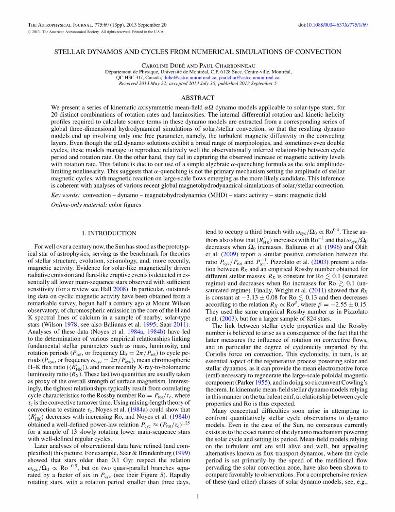
where, as before, angular brackets indicate an average in lon-gitude and time over the statistically stationary phase of thesimulations. Figure 6 shows kinetic helicity profiles for thesame subset of nine simulations as in Figure 3. In all cases, ki-netic helicity is predominantly negative (positive) in the northern(southern) hemisphere, as expected from the hemispheric depen-dency of the Coriolis force imparting cyclonicity on convectiveupdrafts and downdrafts. A sign change is also present at thebase of the convection zone, reflecting the spreading of convec-tive downdrafts impinging on the stable fluid layer underlyingthe convection zone. Helicity increases with increasing thermalforcing and typically peaks at high latitudes, with a secondaryextremum at low latitudes that gradually disappears as rotationincreases.

We now have in hand the ingredients required for theconstruction of kinematic mean-field αΩ dynamo models, towhich we now turn.

4

The Astrophysical Journal, 775:69 (13pp), 2013 September 20 Dube & Charbonneau

Figure 3. Differential rotation profiles in a meridional plane for a subset of 9 out of the 20 hydrodynamical simulations. All profiles are normalized according to therotation rate of their stable layer Ω0. The rotation rate increases from left to right (Ω0/Ω = 0.5, 1, and 3) and the timescale for thermal forcing from bottom to top(ts = 1, 5, and 20). The color scale goes from black (slower than the stable layer) to white (faster than the stable layer). Note the use of a different color scale for eachrotation rate. The Rossby number is indicated above each panel. The dashed line indicates the base of the convectively unstable fluid layers. Most simulations presentsolar-like surface differential rotation profile characterized by polar deceleration and equatorial acceleration, but isocontours of angular velocity show too strong analignment with the rotation axis, as compared to helioseismic inversions of the solar internal differential rotation. This alignment is most pronounced at small thermalforcing timescales or high rotation rates, but here does not show a clear relationship to Rossby number.

(A color version of this figure is available in the online journal.)

3. MEAN-FIELD αΩ DYNAMO

We restrict ourselves here to the simplest form of mean-fielddynamo applicable to the Sun, namely, a kinematic axisym-metric αΩ model. The mean (large-scale and axisymmetric)magnetic field is first expressed through a large-scale toroidalmagnetic component B(r, θ, t) and toroidal vector potentialA(r, θ, t) defining the poloidal magnetic component:

〈B〉(r, θ, t) = ∇ × (A(r, θ, t)eφ) + B(r, θ, t)eφ. (6)

Similarly, the mean (axisymmetric) zonal flow is retained as theonly large-scale flow in the model and is expressed in terms of

an angular velocity of (differential) rotation:

〈u〉(r, θ ) = �Ω(r, θ )eφ, (7)

with � = r sin θ . This mean differential rotation profile isconsidered steady in the dynamo solutions computed below. Inthe αΩ limit, the dimensionless evolution equations for A and Bthen take the form

∂A

∂t= η

(∇2 − 1

� 2

)A + CααB, (8)

5

The Astrophysical Journal, 775:69 (13pp), 2013 September 20 Dube & Charbonneau

Figure 4. Differential rotation contrast ΔΩ/Ω0 vs. rotation rate Ω0. Codingof symbols and lines as in Figure 2, with the few open symbols identifyingsimulations without equatorial acceleration. The best power-law fit is ΔΩ/Ω0 ∝Ω−0.56

0 with all points, and ΔΩ/Ω0 ∝ Ω−0.690 (fit not shown) if simulations

without equatorial acceleration are omitted.

(A color version of this figure is available in the online journal.)

∂B

∂t= η

(∇2 − 1

� 2

)B +

1

�

(dη

dr

)∂(�B)

∂r

+ CΩ� (∇ × Aeφ) · (∇Ω), (9)

with all lengths expressed in units of the solar radius R, andtime in units of the magnetic diffusion time τD = R2/η0, η0being a reference value for the (turbulent) magnetic diffusivityin the convective envelope. The above form of the αΩ dynamoequations leaves open the possibility that the net (turbulent)magnetic diffusivity depends on depth in the model.

In this so-called αΩ framework, shearing by differentialrotation is the sole source term for the toroidal magneticcomponent, while the αB term in Equation (8) is the sole sourcecontribution for the poloidal magnetic field and corresponds tothe turbulent emf provided by the small-scale flow. In termsof the full tensorial relation linking the turbulent emf to themean magnetic field in the more general case, the coefficientα corresponds to the φφ component of the full α-tensor (see,e.g., Moffatt 1978, Section 9; Charbonneau 2010, Section 4.2,and references therein). The strength of the two source terms ismeasured by the dimensionless dynamo numbers

Cα = α0R

η0, CΩ = Ω0R

2

η0, (10)

where α0, Ω0, and η0 are characteristic scaling values.In the present context the differential rotation profile is

extracted directly from the HD simulations described in thepreceding section (viz., Figure 3). For the α-coefficient inEquation (8) we make use of an analytical result obtained underthe so-called SOCA (Rempel 2009, Section 3.4.3; Ossendrijveret al. 2001; Ossendrijver 2003), which links the diagonal,isotropic component of the α-tensor to the kinetic helicity:

α = −τ

3〈u′ · ∇ × u′〉 = −τ

3hυ, (11)

Figure 5. Variation of ΔΩ with Ro−1. Colors, symbols, and lines as in Figure 4.The best power-law fit is ΔΩ ∝ Ro−0.27 including all points, or ΔΩ ∝ Ro−0.19

neglecting simulations without equatorial acceleration (fit now shown). Therelatively small range in log ΔΩ and large scatter give limited meaning to thesefits, but the non-monotonic variation of log ΔΩ with Ro−1 has an observationalcounterpart (see the text).

(A color version of this figure is available in the online journal.)

with τ the correlation time of the turbulence and hυ the meankinetic helicity, which is also extracted from our HD simulations(viz., Figure 6). Following Brown et al. (2010) and Racine et al.(2011), the correlation time is estimated as:

τ (r) = Hρ(r)

u′rms(r)

, (12)

where Hρ is the density scale of the background stratification andu′

rms is the rms average (zonally, latitudinally, and temporally) ofthe small-scale part of the velocity. Working with a simulationof solar convection computed with the MHD version of EULAG(see Smolarkiewicz & Charbonneau 2013), Racine et al. (2011)could show that Equation (11) yields a surprisingly goodrepresentation of the αφφ tensor component directly extractedfrom their simulation (see their Figure 15 and accompanyingdiscussion). The MHD simulation analyzed by these authors isotherwise identical to our HD simulation r1t20 in Table 1. Inwhat follows we assume that this good agreement carries overto other values of rotation rate and thermal forcing.

The only remaining unknown in the model is the turbulentdiffusivity. SOCA also provides an estimate for this quantity,namely:

η0 = τ

3(u′

rms)2. (13)

This value, here taken at mid-convective zone depth and listedin Column 8 of Table 1, is assumed constant throughout theconvection zone and is smoothly matched to a lower diffusivityin the underlying core (see Simard et al. 2013, Section 2.3). Fornumerical convenience we set this turbulent diffusivity contrastto Δη = 10. Measurements of turbulent diffusivity in numericalsimulations suggest that SOCA estimates are actually quiterobust (Courvoisier et al. 2009).

The η0 values listed in Table 1 are at the very high end ofthe range of values obtained by mixing-length estimates foru′

rms. Simard et al. (2013), by an order-of-magnitude analysis ofthe turbulent emf expansion characterizing the MHD simulationanalyzed in Racine et al. (2011), estimated that the above SOCA

6

The Astrophysical Journal, 775:69 (13pp), 2013 September 20 Dube & Charbonneau

Figure 6. Kinetic helicity profiles in a meridional plane for the same subset of nine simulations as in Figure 3: Ω0/Ω = 0.5, 1, 3 from left to right, and forcingtimescale 20, 5, 1 solar days from top to bottom. The color scale indicates the magnitude and sign of hυ in m s−2, with the range increasing from top to bottom.The Rossby number is indicated above each panel. Typically, helicity peaks in polar regions, with secondary extrema appearing at low latitudes. Helicity is negative(positive) in the northern (southern) hemisphere and changes sign near the base of the convection zone, due to the spearing of downward plumes impinging on theunderlying stably stratified fluid layer.

(A color version of this figure is available in the online journal.)

expression for η0 overestimates the true diffusivity by a factorof about 20. The difference is important, because the valueof diffusivity sets the magnetic diffusion time τD = R2/η0,in turn used as a time unit in scaling the dynamo equation.Consequently, the cycle periods characterizing the dynamosolutions to be discussed in the following section scale inverselywith the adopted value of η0.

With the turbulent diffusivity in hand, the αΩ dynamomodel defined by Equations (8) and (9) no longer involvesany adjustable parameters or functionals. However, with anα-coefficient independent of the magnetic field strength, the αΩdynamo equations are linear in A and B, and dynamo action willlead to exponential growth or decay, according to the numericalvalue of the total dynamo number D ≡ CΩ × Cα . We adoptedthe following strategy. First, for each set of differential rotation

and kinetic helicity profile extracted from a simulation, wedetermine the critical dynamo number Dcrit at which an initialfield neither grows nor decays (listed in Column 9 in Table 1and determined to an accuracy of ±5%). Then, we arbitrarilyfix Cα = 12.5 and choose CΩ such that D = CαCΩ = 1.5Dcrit.Finally, we introduce an ad hoc amplitude-limiting nonlinearityknown as algebraic α-quenching:

α → α

1 + (B/Beq)2, (14)

where Beq ∝ u′rms is the equipartition field strength, the

numerical value of which sets the absolute scale of the magneticfield amplitude in the dynamo calculations. For an αΩ modelwith α-quenching, the value of Beq does not affect cycle period,

7

The Astrophysical Journal, 775:69 (13pp), 2013 September 20 Dube & Charbonneau

Figure 7. Spatiotemporal evolution of the zonally averaged toroidal magnetic field for the αΩ model constructed from reference solution r1t20. The top panel showsa time–latitude diagram at r/R = 0.85, and the bottom panel shows a time–radius diagram at 22.◦5 latitude, where the dashed line indicates the base of the convectivezone. The color scale codes the magnetic field strength, normalized to the maximum absolute value shown above each panel. The input parameter values used areCΩ = 1050, Cα = 12.5, and Δη = 10. The resolution used is Nθ × Nr = 96 × 128. The primary dynamo mode (greater magnetic intensity) is concentrated at lowlatitudes, is antisymmetric with respect to the equator, and migrates poleward in the course of the cycle. There is a second, shorter cycle at polar latitudes. Both modesbehave similarly in a time–radius diagram, peaking around r/R ≈ 0.9 and migrating upward through the bulk of the convection zone.

(A color version of this figure is available in the online journal.)

but only its magnitude. We adopt a value Beq = 5 kG for thereference simulation r1t20 and scale it according to the ratioof rms convective flow velocity in the other simulations. Underα-quenching, the cycle period shows little dependence on theadopted value for dynamo number D.

The numerical solution of Equations (8) and (9) in themeridional plane is carried out using the finite element-basedmodel described in Charbonneau et al. (2005) and Simard et al.(2013), on a spatial mesh of Nθ × Nr = 96 × 128 bilinearelements. Bilinear interpolation is used to evaluate on thismesh the angular velocity and α-coefficient profiles extractedfrom the numerical simulations. The dynamo simulations areinitialized using a very weak toroidal magnetic field and areintegrated in time until the magnetic energy stabilizes. Allanalyses reported upon below extract cycle characteristics fromthis stationary phase, excluding the initial transient phase ofexponential growth.

4. RESULTS

4.1. Validation

We first examine in some detail the αΩ model constructedfrom our reference “solar” simulation r1t20 (Ω0 = 2.5972 ×10−6 rad s−1 (⇒ Prot = 28 days) and ts = 20 s.d.). Figure 7shows a time–latitude diagram of the mean toroidal field atmid-convection depth (r/R = 0.85) and a radius–time diagramof the same at latitude +22.5 deg. This solution exhibits twodistinct dynamo modes, both of roughly the same amplitudeand peaking within the convection zone at r/R ≈ 0.9, the firstat low latitudes and the other, with a frequency almost four timeshigher, in the polar region. The origin of this “double-dynamo”behavior can be traced to the spatial profiles of differentialrotation and kinetic helicity: the former usually show a strongshear region at low latitudes and a weaker shear near thepoles (see the top-center panel in Figure 3), while the latterpeak in polar regions and often show a secondary peak at

mid- to low latitudes (see the top-center panel in Figure 6).The low (high) latitude mode exhibits poleward (equatorward)propagation, which is precisely the pattern expected from theParker–Yoshimura sign rule for dynamo waves feeding onpositive (negative) radial shear and a positive (negative) α-effectin the northern (southern) hemisphere. Both modes also exhibitpropagation directed radially outward, again as expected fromthe sign of the local latitudinal shear.

Figure 8 shows, in the same format as Figure 7, the spa-tiotemporal evolution of the zonally averaged toroidal magneticcomponent in a EULAG-MHD simulation carried out at the so-lar rotation rate and using the same thermal forcing timescale asour reference HD simulation r1t20. This global MHD simula-tion generates a large-scale magnetic cycle within its convectionzone that shows some striking similarities to the mean-field αΩdynamo solution of Figure 7: a dynamo mode concentratedin equatorial regions, peaking at latitude ∼25 deg and depthr/R � 0.9, antisymmetric about the equator and propagatingpoleward and upward. Close examination of Figure 8 also re-veals a low-amplitude polar mode, although now with a fre-quency comparable to its low-latitude counterpart, and showingat best a hint of equatorward propagation. These dissimilaritiesnotwithstanding, the morphological resemblance between thefully dynamical three-dimensional global MHD simulation andthe much simpler axisymmetric kinematic αΩ dynamo solutionremains striking and lends confidence to our adopted modelingapproach.

4.2. More Dynamo Solutions Across Parameter Space

Henceforth the strategy is in principle simple: we computeαΩ dynamo solutions using the differential rotation profilesand α-coefficients constructed from the helicity profiles asso-ciated with each of our 20 HD simulations of convection. Wethen extract time–latitude diagrams of the axisymmetric meantoroidal magnetic component at mid-convection-zone depth in

8

The Astrophysical Journal, 775:69 (13pp), 2013 September 20 Dube & Charbonneau

Figure 8. Spatiotemporal evolution of the zonally averaged toroidal magnetic field for a EULAG-MHD simulation otherwise identical to the r1t20 simulation usedto generate the αΩ dynamo solution of Figure 7. The top panel shows a time–latitude diagram at r/R = 0.88 and the bottom panel a time–radius diagram at 25◦latitude; the dashed line indicates the base of the convective zone. The color scale denotes the magnetic field strength in Tesla. A small explicit magnetic dissipationof η = 106 m2 s−1 is included in this MHD simulation, executed at a resolution of Nφ × Nθ × Nr = 256 × 128 × 97. The cycle is located at low latitudes and is alsoantisymmetric relative to the equator. In a time–radius diagram, the cycle reaches maximum intensity around r/R ≈ 0.9. Comparing this figure to Figure 7 suggeststhat our simplified αΩ model can capture the main features of a global MHD simulation.

(A color version of this figure is available in the online journal.)

each model. From these time–latitude diagrams we then measurethe cycle period, Pcyc (half the magnetic period). This is listedin Column 10 of Table 1. In some cases, as with the r1t20solution of Figure 7, there are two distinct activity cycles, inwhich case the secondary cycle period is denoted Pcyc(2) and islisted in Column 11 of Table 1. The periods are all much shorterthan observed, but this is a direct consequence of the very highmagnetic diffusivity values used in the αΩ dynamo model, asper Equation (13). Reducing it by a factor of 20, as suggestedby the analysis of Simard et al. (2013), would bring them muchcloser to observations. Two αΩ models actually generate non-oscillatory, steady magnetic solutions, in which case no periodis listed in Table 1. Finally, for each solution, we also computethe temporally averaged magnetic energy Emag, the result beinglisted in the rightmost column of Table 1.

All that remains is to correlate cycle period and magneticenergy to global model properties such as rotation rates, Rossbynumbers, etc. This seemingly straightforward approach is com-plicated by the fact that the morphology of the dynamo mode(s)can vary significantly across our parameter space, even thoughthe latter is relatively restricted in span (a factor of six in rotationrate, and approximately eight in convective luminosity). This isillustrated in Figure 9, showing dynamo solutions for a subset ofour simulations, namely, r0.5t5, r0.5t20, r1t50, and r3t20.Figure 9(A) illustrates a single-cycle dynamo solution peak-ing at mid-latitudes and exhibiting equatorward propagation,symmetric about the equatorial plane. As with the solution ofFigure 7, the dynamo mode peaks around r/R � 0.9 andshows upward propagation. Figure 9(B), in contrast, shows asolution characterized by a cycle peaking at high latitudes.Moreover, this dynamo mode now peaks slightly below thecore–envelope interface and shows only mild upward propa-gation. Figure 9(C) shows a dual-mode dynamo solution, asin Figure 7, this time with the high-latitude mode having aperiod some six times longer than the low-latitude mode andmodulating the latter’s amplitude. Here the low-latitude cyclepeaks at mid-depth within the convection zone, while the high-latitude mode peaks again slightly beneath the core–envelope

interface, propagating upward in the convection zone and pen-etrating deeply into the tachocline. Figure 9(D), finally, showsa short-period, equatorially concentrated single-mode dynamosolution symmetric about the equatorial plane, propagating pole-ward and peaking at r/R � 0.95, in the outer reaches of theconvection zone.

How can this wide disparity in spatiotemporal evolutionbe explained? The most prominent variation occurs with theappearance of equatorial acceleration as one transits from slowlyrotating models (Ω0/Ω � 0.75) to more rapid rotation. Thepeak rotational shear, and thus the dynamo mode, transits frommid- to low latitudes (cf. panels A, B and C, D of Figure 9).The r1t50 dynamo solution of Figure 9(C) is unique amongthe set in producing a low-latitude dynamo mode propagatingtoward and peaking at the equator; this can be traced to the (non-solar) differential rotation profile, where the region of equatorialacceleration peaks deep in the convection zone, leading to anegative radial gradient of angular velocity in the outer half ofthe convection zone. In conjunction with a positive α-effect inthe northern hemisphere, this leads to equatorward propagationof dynamo waves, as per the Parker–Yoshimura sign rule. Dualhigh + low dynamo modes occur in five simulations, all atrotation rates solar or close (see Table 1). Their absence athigh rotation rate is likely associated with the disappearanceof polar deceleration in the most rapidly rotating simulations(see rightmost panels in Figure 3). Secondary modes, whenthey occur, tend to peak at high latitudes and near the base ofthe convection zone, reflecting the action of the strong radialshear often present there (see Figure 3). No particular pattern isapparent regarding the amplitude and period ratios on rotationrate or thermal forcing. Equatorial symmetry/antisymmetry alsovaries across parameter space, again with no obvious patternwith rotation rate or thermal forcing. Observational evidence fora “double dynamo” actually exists in the case of the Sun, in theform of a ∼2 yr modulation superimposed on the primary 11 yractivity cycle detected in a variety of solar activity measures(see, e.g., Mursula et al. 2003; Fletcher et al. 2010; Simonielloet al. 2013, and references therein). However, whether this

9

The Astrophysical Journal, 775:69 (13pp), 2013 September 20 Dube & Charbonneau

Figure 9. Time–latitude diagram of the zonally averaged toroidal magnetic field for simulations (A) r0.5t5, (B) r0.5t20, (C) r1t50, and (D) r3t20. Each panelshows a time–latitude diagram at r/R = 0.85. The color scale denotes the magnetic field strength normalized to the peak value given above each panel. The inputparameter values used are the same as in Figure 7 except for CΩ, which is equal to 366 for (A), 1980 for (B), 5100 for (C), and 2280 for (D). Even in the context of ourvery simple αΩ formulation, and even with the relatively limited range of our two-dimensional parameter space, a wide variety of dynamo modes can be produced,with varying cycle lengths, modes peaking at low, mid-, or high latitudes, propagating either poleward or equatorward, symmetric or antisymmetric with respect to theequatorial plane.

(A color version of this figure is available in the online journal.)

solar behavior can be legitimately linked to that observed inthe αΩ dynamo calculations considered here remains to beinvestigated.

Most simulations produce a peak toroidal field of a fewkiloGauss. This constancy, a priori surprising given the widerange of morphology seen in the dynamo modes, is a directconsequence of the algebraic α-quenching formulae introducedto limit the cycle amplitude. The relatively wide range inmagnetic energy apparent in the rightmost column of Table 1reflects primarily the spatial extent of the dynamo modes,in particular the presence or absence of magnetic fields inthe radiative core underlying the convection zone, rather thanvariations on overall magnetic field strength.

4.3. Cycle Relationships

We now turn to the relationships existing—or not—betweencycle characteristics such as cycle period and magnetic energyon fundamental parameters such as the rotation rate, and theirderivatives such as the Rossby number Ro. We do so in a mannerresembling as much as possible the relationships establishedobservationally. Except when considering magnetic energies, inwhat follows we exclude from consideration the two simulations

r0.5t1 and r3t1, which produce non-oscillatory dynamomodes.

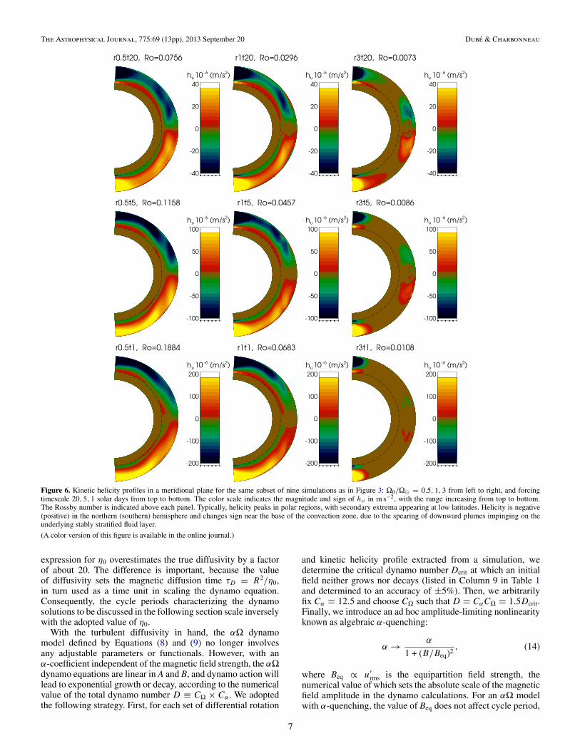
Figure 10 shows the variation of the ratio Pcyc/Prot with1/Prot. On this and following plots, as before symbols are color-coded according to rotation rate and linked with lines styledaccording to the value of the thermal forcing timescale. Ournumerical data can be reasonably well fit by a power law of theform

Pcyc

Prot∝ P −1.47

rot (15)

(gray solid line in Figure 10). This ratio is clearly increasingwith increasing rotation rate, which is similar to the variationestablished observationally by Baliunas et al. (1996) and Olahet al. (2009) and is also consistent with Saar & Brandenburg(1999). However, our power-law fit yields an index of −1.47,which is significantly steeper than the results of Baliunas et al.(1996, index −0.74) and Olah et al. (2009, index −0.81±0.05).That such a relatively well-defined power-law relationshipshould arise in our model is a priori surprising, given the widerange of dynamo morphologies occurring across our parameterspace. This indicates that the general decrease of the cycle periodwith increasing rotation rate is a very robust property of αΩ

10

The Astrophysical Journal, 775:69 (13pp), 2013 September 20 Dube & Charbonneau

Figure 10. Variation of the ratio Pcyc/Prot with 1/Prot. Circles and asterisksrepresent main and secondary cycle (Pcyc and Pcyc(2) in Table 1), respectively.The vertical dotted lines link secondary cycles to primary ones. Asterisks weredisplaced horizontally for clarity. Other colors and lines as in Figure 2. Thepower-law fit (gray line) neglects secondary cycles and yields Pcyc/Prot ∝P −1.47

rot . This is coherent with, but steeper than, the results of Baliunas et al.(1996, slope of −0.74) and Olah et al. (2009, slope of −0.81 ± 0.05).

(A color version of this figure is available in the online journal.)

Figure 11. Ratio ωcyc/Ω0 vs. Ro−1. Symbols and lines as in Figure 10. Oneasterisk (blue) was displaced horizontally for clarity. Again, the power-lawfit neglects secondary cycles and gives the result ωcyc/Ω0 ∝ Ro0.96. This isdifferent from what was previously found by Saar & Brandenburg (1999):two almost parallel branches with ωcyc/Ω0 ∝ Ro−0.5 and a third branch withωcyc/Ω0 ∝ Ro0.4 for very active stars (Prot < 3 days).

(A color version of this figure is available in the online journal.)

dynamo models, which does not depend sensitively on detailsof the dynamo mode. Figure 11 shows the variation of effectivelythe same ratio, now expressed in terms of frequencies rather thanperiods, with the inverse Rossby number. Saar & Brandenburg(1999) constructed similar plots and obtained ωcyc/Ω0 ∝ Ro−0.5

for most stars, but ωcyc/Ω0 ∝ Ro0.4 for very active stars(Prot < 3 days). Here, one observes significant scatter in thesimulation data, although a clear downward trend is present. A

Figure 12. Emag vs. Ro−1. Colors and lines as in Figure 2. The best power-lawfit is Emag ∝ Ro0.73. We would have expected this relationship to be similarto those linking 〈R′

HK〉 or RX to the Rossby number since those parametersare linked to the magnetic activity cycle. Our correlation is opposite to whatwas previously found in literature (see Noyes et al. 1984a; Saar & Brandenburg1999; Pizzolato et al. 2003; Wright et al. 2011).

(A color version of this figure is available in the online journal.)

power-law fit now yields:

ωcyc

Ω0∝ Ro0.96. (16)

The discrepancy is curious, given that our model succeeds ratherwell in reproducing the observed trend in the Pcyc/Prot versusProt relationship. It probably hinges on the aforementionedcomplex dependency of our Rossby number, as defined byEquation (3), which contains an implicit dependency on rotationhidden within u′

r rms (see Table 1 and Figure 1).We also investigated the dependence of magnetic energy on

the Rossby number. Since chromospheric and coronal activitycan be linked to stellar magnetic activity, we would expectto obtain at least qualitatively similar relationships for themagnetic energy, the mean chromospheric H–K flux ratio 〈R′

HK〉,and the X-ray-to-bolometric luminosity ratio RX. Numerousobservational studies (Noyes et al. 1984a; Saar & Brandenburg1999; Pizzolato et al. 2003; Wright et al. 2011) have revealed anincrease of 〈R′

HK〉 and RX with increasing Ro−1 holding up to asaturation value beyond which the dependence on Ro effectivelyvanishes.

Despite wide scatter in our simulation data, Figure 12 showsthat our magnetic energies tend to decrease with increasingRo−1. A power-law fit on these simulation data gives

Emag ∝ Ro0.73. (17)

This trend is completely incoherent with the aforementioned ob-servational inferences. This discrepancy is in all likelihood dueto the simple kinematic α-quenching algebraic nonlinearity usedto limit the amplitude of the dynamo modes (viz., Equation (14)).In the αΩ model defined in Section 3 above, the magnetic ampli-tude is entirely set by the adopted equipartition field strength inEquation (14), implying that the reduction of the α-effect isthe only nonlinear feedback mechanism present. Recent globalMHD simulations of solar convection (e.g., Racine et al. 2011)have uncovered no compelling evidence for α-quenching, and

11

The Astrophysical Journal, 775:69 (13pp), 2013 September 20 Dube & Charbonneau

suggest instead that magnetic back-reaction on large-scale flows,including differential rotation, may be in fact the primaryamplitude-limiting nonlinearity (see Brown et al. 2008, 2010).

5. DISCUSSION

In this paper, we have extracted profiles of differential rota-tion and kinetic helicity from a set of 20 global HD simulationsof stellar convection at varying rotation rates and luminosityand have used these profiles as input into a simple kinematic ax-isymmetric αΩ mean-field dynamo model subjected to algebraicα-quenching. This procedure is validated by comparing one ofour dynamo solutions to the magnetic cycle developing in a fullyMHD global simulation of convection carried out at the samerotation rate and thermal forcing. Extracting magnetic cycle pe-riods from these dynamo solutions then allows us to constructthe equivalent of some observationally inferred relationshipslinking cycle period and amplitude to stellar parameters such asrotation rate, luminosity, and associated Rossby number.

Through this modeling approach we do manage to capturesome important characteristics of stellar activity cycles, inparticular the observationally inferred power-law relationshiplinking the ratio Pcyc/Prot to the rotation rate (Baliunas et al.1996; Saar & Brandenburg 1999; Olah et al. 2009). However,we fail to capture the observationally inferred dependence onRossby number (Noyes et al. 1984a; Pizzolato et al. 2003; Saar2011; Wright et al. 2011). At least two factors likely contributeto this failure: our use of a fixed background structural modelfor the numerical simulations (more on this below), and theobservational or semi-empirical definition of the Rossby numberused in observational analyses, which is typically obtained fromturning luminosity into convective flow speed, or estimatingconvective turnover times from models or simulations, underthe assumption that convection is unaffected by rotation. Thisis certainly not the case in our HD simulations (viz., Figures 1and 2 herein).

Clearly, much could be improved in our overall modelingapproach, in order to strengthen the comparison to stellar cycleobservations. The use of differential rotation profiles extractedfrom a purely HD simulation was motivated in part by thefact that these are much less demanding computationally andattain a statistically stationary state much more rapidly thantheir MHD equivalent. Yet, many published simulations of solarconvection have shown that even when no large-scale magneticcycle develops, the Maxwell stresses associated with small-scalemagnetic field reduce the magnitude of differential rotation, ascompared to purely HD simulations otherwise identical (e.g.,Brown et al. 2010 and references therein). Since we run all ourαΩ dynamo models at 1.5 times the critical dynamo number,a general decrease of differential rotation should not affectcritically the results presented here as long as this decreaseis more or less homogeneous spatially. This issue nonethelessdeserves further investigation.

Another potentially important aspect we have not exploredin the present work is the influence of global stellar structuralparameters. More specifically, all HD simulations and dynamomodels considered here are executed in fluid spheres of fixedsolar radius, gravity, and convection zone depth. Workingwith the Kitchatinov & Rudiger (1999) model for differentialrotation and meridional flow, Kuker et al. (2011) have shownthat relatively small variations in the depth of the convectionzone can produce large departures from the ΔΩ versus Ω0relationship characterizing their model at fixed convection zonedepth. Investigating these structural effects is possible within

the modeling approach developed here and should definitely becarried out.

Despite the wide range of morphologies for the αΩ dynamomodes generated from our ensemble of simulations, the varia-tions of magnetic cycles with rotation rate are found to followa power-law relationship of the same general form as inferredobservationally. More specifically, an increase of the simula-tions’ rotation rate leads to a marked decrease of the Pcyc/Protratio, although more pronounced than observed. Our results thusindicate that this trend is a very robust property of kinematicmean-field αΩ dynamo models, using α-quenching as the soleamplitude-limiting nonlinearity (see also Tobias 1998). Interest-ingly, this relationship is one that could not be reproduced, evenas a general trend, in the similar numerical experiments car-ried out by Jouve et al. (2010), using a flux-transport dynamomodel, where the primary determinant of the cycle period isthe meridional flow speed. Taken jointly, these results highlightthe fact that determinations of stellar cycle periods in well-characterized samples (in terms of mass, age, rotation rate) canpotentially provide strong discriminants on various classes ofdynamo models.

To the extent that magnetic energy computed from the dy-namo solution can be taken as a proxy of the amplitude of surfacemagnetic activity, the present modeling work fails in capturingthe observed rise of activity level with decreasing Rossby num-ber or increasing rotation rate, as inferred observationally. Theorigin of this discrepancy lies in part with the fact that we optedto run all αΩ dynamo simulations at 1.5 times the critical dy-namo number, but the primary cause is more likely our use ofalgebraic α-quenching as the sole amplitude-limiting nonlinear-ity. Racine et al. (2011) attempted to measure α-quenching inan MHD version of simulation r1t20 herein, which produceda large-scale magnetic cycle, but found that the components ofthe α-tensor extracted from the simulation showed very little,if any, temporal variation on the timescale of their large-scalemagnetic cycle. On the other hand, the pole-to-equator angularvelocity contrast was found to decrease by a factor of three ingoing from the purely HD simulation to its MHD descendant.A similar pattern was observed in many other global numericalsimulations of solar convection (e.g., Brown et al. 2010, andreferences therein) and is coherent with the idea, establishedalready by Gilman (1983) on the basis of his pioneering con-vection simulations, that back-reaction on the large-scale flowsis the primary amplitude-limiting mechanism for this type ofconvective dynamo. Once again, this highlights the importanceof well-characterized stellar samples in measuring stellar sur-face magnetic activity, as this holds important clues regardingthe nonlinear saturation of the underlying dynamos.

This work was made possible by Calcul Quebec and sup-ported by Canada’s Natural Sciences and Engineering Re-search Council, Research Chair Program, and by the CanadianSpace Agency’s Space Science Enhancement Program (grantNo. 9SCIGRA-21). C.D. is also supported in part through agraduate fellowship from the Universite de Montreal’s physicsdepartment and through a graduate fellowship from the Fondsde recherche du Quebec—Nature et technologies.

REFERENCES

Baliunas, S. L., Donahue, R. A., Soon, W. H., et al. 1995, ApJ, 438, 269Baliunas, S. L., Nesme-Ribes, E., Sokoloff, D., & Soon, W. H. 1996, ApJ,

460, 848Ballot, J., Brun, A. S., & Turck-Chieze, S. 2007, ApJ, 669, 1190

12

The Astrophysical Journal, 775:69 (13pp), 2013 September 20 Dube & Charbonneau

Barnes, J. R., Collier Cameron, A., Donati, J.-F., et al. 2005, MNRAS,357, L1

Brown, B. P., Browning, M. K., Brun, A. S., Miesch, M. S., & Toomre, J.2008, ApJ, 689, 1354

Brown, B. P., Browning, M. K., Brun, A. S., Miesch, M. S., & Toomre, J.2010, ApJ, 711, 424

Brun, A. S., & Toomre, J. 2002, ApJ, 570, 865Charbonneau, P. 2010, LRSP, 7, 3Charbonneau, P., & Saar, S. H. 2001, in ASP Conf. Ser. 248, Magnetic

Fields Across the H-R Diagram, ed. G. Mathys, S. K. Solanki, & D. T.Wickamasinghe (San Francisco, CA: ASP), 189

Charbonneau, P., St-Jean, C., & Zacharias, P. 2005, ApJ, 619, 613Courvoisier, A., Hughes, D. W., & Tobias, S. M. 2009, JFM, 627, 403Elliott, J. R., & Smolarkiewicz, P. K. 2002, IJNMF, 39, 855Fletcher, S. T., Broomhall, A.-M., Salabert, D., et al. 2010, ApJL, 718, L19Ghizaru, M., Charbonneau, P., & Smolarkiewicz, P. K. 2010, ApJL, 715, L133Gilman, P. A. 1977, GApFD, 8, 93Gilman, P. A. 1983, ApJS, 53, 243Guerrero, G., Smolarkiewicz, P. K., Kosovichev, A., & Mansour, N. 2013, in

IAU Symp. 294, Solar and Astrophysical Dynamos and Magnetic Activity,ed. A. G. Kosovichev, E. M. de Gouveia Dal Pino, & Y. Yan (Cambridge:Cambridge Univ. Press), 417

Hall, J. C. 2008, LRSP, 5, 2Howe, R. 2009, LRSP, 6, 1Jouve, L., Brown, B. P., & Brun, A. S. 2010, A&A, 509, A32Kapyla, P., Mantere, M. J., Guerrero, G., Brandenburg, A., & Chatterjee, P.

2011, A&A, 531, A162Kitchatinov, L. L., & Rudiger, G. 1999, A&A, 344, 911Kuker, M., Rudiger, G., & Kitchatinov, L. L. 2011, A&A, 530, A48Miesch, M., Brun, A. S., & Toomre, J. 2006, ApJ, 641, 618

Miesch, M., Elliott, J. R., Toomre, J., et al. 2000, ApJ, 532, 593Moffatt, H. K. 1978, Magnetic Field Generation in Electrically Conducting

Fluids (Cambridge: Cambridge Univ. Press)Mursula, K., Zieger, B., & Vilppola, J. H. 2003, SoPh, 212, 201Nandy, D., & Martens, P. C. H. 2007, AdSpR, 40, 891Noyes, R. W., Hartmann, L. W., Baliunas, S. L., Duncan, D. K., & Vaughan,

A. H. 1984a, ApJ, 279, 763Noyes, R. W., Weiss, N. O., & Vaughan, A. H. 1984b, ApJ, 287, 769Olah, K., Kollath, Z., Granzer, T., et al. 2009, A&A, 501, 703Ossendrijver, M. 2003, A&ARv, 11, 287Ossendrijver, M., Stix, M., & Brandenburg, A. 2001, A&A, 376, 713Parker, E. N. 1955, ApJ, 122, 293Pizzolato, N., Maggio, A., Micela, G., Sciortino, S., & Ventura, P. 2003, A&A,

397, 147Prusa, J. M., Smolarkiewicz, P. K., & Wyszogrodzki, A. A. 2008, CF, 37, 1193Racine, E., Charbonneau, P., Ghizaru, M., Bouchat, A., & Smolarkiewicz, P. K.

2011, ApJ, 735, 46Rempel, M. 2009, in Heliophysics: Plasma Physics of the Local Cosmos, ed. C.

J. Schrijver & G. L. Siscoe (Cambridge: Cambridge Univ. Press), 42Saar, S. H. 2011, in IAU Symp. 273, The Physics of Sun and Star Spots, ed.

D. P. Choudhary & K. G. Strassmeier (Cambridge: Cambridge Univ. Press),61

Saar, S. H., & Brandenburg, A. 1999, ApJ, 524, 295Simard, C., Charbonneau, P., & Bouchat, A. 2013, ApJ, 768, 16Simoniello, R., Jain, K., Tripathy, S. C., et al. 2013, ApJ, 765, 100Smolarkiewicz, P. K., & Charbonneau, P. 2013, JCP, 236, 608Tobias, S. M. 1998, MNRAS, 296, 653Wilson, O. C. 1978, ApJ, 226, 379Wright, N. J., Drake, J. J., Mamajek, E. E., & Henry, G. W. 2011, ApJ,

743, 48

13