Stellar Dynamics and Structure of Galaxies - …vasily/Lectures/SDSG/sdsg_2_poisson.pdf · Galaxies Part II Potentials from density distribution Poisson’s Equation Gauss’s Theorem

Galaxies Part II

Potentials from densitydistribution

Profiles and potentials

Stellar Dynamics and Structure of GalaxiesDerivation of potential from density distribution

Vasily [email protected]

Institute of Astronomy

Lent Term 2016

1 / 41

Galaxies Part II



Outline I

1 Potentials from density distributionPoisson’s EquationGauss’s TheoremEdwin Hubble’s classification of galaxiesDeriving potentials of spherical systems

2 Profiles and potentialsModified Hubble profilePower law density profileProjected density → spherical density

2 / 41

Galaxies Part II


Poisson’s Equation

Gauss’s Theorem

Edwin Hubble’sclassification of galaxies

Deriving potentials ofspherical systems


Potentials from density distributionPoisson’s Equation

Poisson’s equation relates ρ(r) to Φ(r). �

�Already covered in the Astrophysical Fluid Dynam-

ics course - here we explore it a little further

To determine the force due to a given density distribution ρ(r ′) we split it into manypoint masses of size

dm′ = ρ(r ′)d3r′ at r′

Newtonian gravity is linear, so just add up the forces

f(r) = −∫

Gdm′

|r − r′|3(r − r′)

or since we want the total potential add up the individual contributions

Φ(r) =

∫ ∫ ∫Gρ(r′)d3r′

|r − r′|�� As an exercise, show that ∇r1|r′−r| = r′−r

|r′−r|3 , and hence f(r) = −∇Φ

3 / 41

Galaxies Part II



Gauss’s Theorem





Consider

∇2Φ(r) = −∫ ∫ ∫

Gρ(r′)∇2r

(1

|r − r′|

)d3r′

⇒ need ∇2r

(1|r−r′|

).

To keep the algebra simple move the origin to r′ (and move back later)�

�for those who want everything in full generality, see

Binney & Tremaine

So we need ∇2( 1r ). For r 6= 0,

∇2

(1

r

)=

1

r2

d

dr

[r2 d

dr

(1

r

)]= 0 trivially

4 / 41

Galaxies Part II



Gauss’s Theorem





But at r = 0 ∇2( 1r ) is undefined. �

�You’ve seen that sort of thing before. Recall that

the Dirac δ-function δ(x) satisfies∫ ε−ε δ(x)dx = 1

So now ask: what is the volume integral of ∇2( 1r ) over a small volume V containing

the origin?

∫ ∫ ∫V

∇2

(1

r

)d3V =

∫ ∫ ∫V

∇ .[∇(

1

r

)]d3V by definition

=

∫ ∫S

n .[∇(

1

r

)]d2S (2.1)

�� Divergence theorem (n - outward normal)∫V d3x∇F =

∫S nF

5 / 41

Galaxies Part II



Gauss’s Theorem





Take V to be a sphere, so n = r, d2S = r2 sin θdθdφ, and have ∇(1/r) = − 1r2 r. Then

∫ ∫ ∫V

∇2

(1

r

)d3V = −

∫ 2π

0

dφ

∫ π

0

sin θdθ

= −4π (2.2)

Since the integral is −4π, and is non-zero only at r = 0, we must therefore have

∇2

(1

r

)= −4πδ(r)

or, going back to the general origin,

∇2

(1

|r − r′|

)= −4πδ(r − r′)

6 / 41

Galaxies Part II



Gauss’s Theorem





Hence

∇2Φ(r) = −G∫ ∫ ∫

ρ(r′)∇2

(1

|r − r′|

)d3r′

= 4πG

∫ ∫ ∫ρ(r′)δ(r − r′) d3r′

= 4πGρ(r) (2.3)

∇2Φ(r) = 4πGρ(r)


7 / 41

Galaxies Part II



Gauss’s Theorem




Gauss’s TheoremApplication of the Divergence Theorem to the Poisson’s Equation

“The integral of the normal component of ∇Φ over any closed surface equals 4πGtimes the mass enclosed within that surface”

To prove this simply take Poisson’s equation and integrate over a volume V containinga mass M.

4πG

∫ρd3r = 4πGM =

∫∇2Φ d3r

=

∫∇ .∇Φ d3r

=

∫∇Φ . n d2S (2.4)

where the last step follows from the divergence theorem.

8 / 41

Galaxies Part II



Gauss’s Theorem




Edwin Hubble’s classification of galaxies

Astrophysical Journal, 64, 321-369 (1926)

9 / 41

Galaxies Part II



Gauss’s Theorem




Edwin Hubble’s classification of galaxies

10 / 41

Galaxies Part II



Gauss’s Theorem




Edwin Hubble’s classification of galaxiesEarly Types

Fundamental plane exists that ties surface brightness, size and LOS velocity dispersion

11 / 41

Galaxies Part II



Gauss’s Theorem




Edwin Hubble’s classification of galaxiesSpirals

Tully-Fisher law exists that ties together circular speed and luminosity12 / 41

Galaxies Part II



Gauss’s Theorem




Edwin Hubble’s classification of galaxiesIrregulars

13 / 41

Galaxies Part II



Gauss’s Theorem




Edwin Hubble’s classification of galaxiesThe Tuning Fork

14 / 41

Galaxies Part II



Gauss’s Theorem




Edwin Hubble’s classification of galaxiesThe Three Pioneers

Albert Einstein, Edwin Hubble, and Walter Adams in 1931 at the Mount WilsonObservatory 100” telescope, in the San Gabriel Mountains of southern California.

15 / 41

Galaxies Part II



Gauss’s Theorem




Edwin Hubble’s classification of galaxiesGalaxy Luminosity Function

In any environment, dwarfs dominate!16 / 41

Galaxies Part II



Gauss’s Theorem




Deriving potentials of spherical systems

�� we can take ρ(r) = ρ(r)

In spherical polars

∇2Φ(r) =1

r2

d

dr

(r2 d

drΦ

)=

1

r

d2

dr2(rΦ)�� Exercise: show the last equality is true

So∇2Φ = 4πGρ

becomes1

r

d2

dr2(rΦ) = 4πGρ,

and, given ρ we can solve for Φ(r).

17 / 41

Galaxies Part II



Gauss’s Theorem




Deriving potentials of spherical systemsHomogeneous Sphere

(a) Homogeneous sphere: ρ(r) = ρ0 for 0 < r < r0, and ρ(r) = 0 for r > r0.So for r < r0, have

1

r

d2

dr2(rφ) = 4πGρ0

d2

dr2(rφ) = 4πGρ0r

d

dr(rφ) = 2πGρ0r

2 + A

rΦ =2

3πGρ0r

3 + Ar + B

Φ(r) =2

3πGρ0r

2 + A +B

r(2.5)

18 / 41

Galaxies Part II



Gauss’s Theorem




Deriving potentials of spherical systemsHomogeneous Sphere�� Φ(r) = 2

3πGρ0r2 + A + B

r

Require that Φ is finite at r = 0, else there is a point mass there, and so B = 0.⇒ Φ(r) = 2

3πGρ0r2 + A for 0 < r < r0.

For r > r0 have1

r

d2

dr2(rΦ) = 0

⇒ rΦ = Cr + D

Φ(r) = C +D

r

WLOG 1 let Φ→ 0 as r →∞ (this is just choosing the zero point of the potential).

⇒ Φ(r) =D

rfor r0 < r

1WLOG=Without Loss Of Generality19 / 41

Galaxies Part II



Gauss’s Theorem




Deriving potentials of spherical systemsHomogeneous Sphere�� Φ(r) = 2

3πGρ0r2 + A for 0 < r < r0

�� Φ(r) = Dr

for r0 < r

Also require Φ to be continuous at r = r0, since ∇Φ=force is finite there, and dΦdr also

continuous (else ∇2Φ = 4πGρ is infinite there).

⇒ 2

3πGρ0r

20 + A =

D

r0

and4

3πGρ0r0 = −D

r20

⇒D = −4

3πGρ0r

30

andA = −2πGρ0r

20

20 / 41

Galaxies Part II



Gauss’s Theorem




Deriving potentials of spherical systemsHomogeneous Sphere

Hence

Potential of a homogeneous sphere

Φ(r) =2

3πGρ0(r2 − 3r2

0 ) 0 < r < r0

= −4

3πGρ0r

30 /r r0 < r (2.6)

Note: Outside the sphere Φ = −GMr as expected, where M = 4

3πρ0r30 .

Newton’s 2nd theorem: “Outside a closed spherical shell of matter, the gravitationalpotential is as if all the mass were at a point at the centre”

21 / 41

Galaxies Part II



Gauss’s Theorem




Deriving potentials of spherical systemsSpherical Shell

(b) Spherical shell ρ(r) = ρ0 for r1 < r < r2 and ρ(r) = 0 otherwise.Newtonian gravity is linear, so this is the same as(1) a uniform sphere density ρ0, radius r2

PLUS(2) a uniform sphere density −ρ0, radius r1.So we can write the answer down. It is

Φ(r) =2

3πGρ0(r2 − 3r2

2 )− 2

3πGρ0(r2 − 3r2

1 ) 0 < r < r1

=2

3πGρ0(r2 − 3r2

2 ) +4

3πGρ0r

31 /r r1 < r < r2

= −4

3πGρ0r

32 /r +

4

3πGρ0r

31 /r r2 < r (2.7)

22 / 41

Galaxies Part II



Gauss’s Theorem





Notes:(1) Inside the cavity 0 < r < r1: Φ(r) = 2

3πGρ0(r2 − 3r22 )− 2

3πGρ0(r2 − 3r21 )

Φ =constant since the r2 terms cancel. Therefore there is no force due to an externalspherically symmetric mass distribution �� Newton’s first theorem

(2) Outside the shell r > r2: Φ(r) = − 43πGρ0r

32 /r + 4

3πGρ0r31 /r

Φ = −GMshell

r

where Mshell = 43πρ0(r3

2 − r31 ) is the mass in the shell

23 / 41

Galaxies Part II



Gauss’s Theorem





Notes:(1) Inside the cavity 0 < r < r1: Φ(r) = 2

3πGρ0(r2 − 3r22 )− 2

3πGρ0(r2 − 3r21 )

Φ =constant since the r2 terms cancel. Therefore there is no force due to an externalspherically symmetric mass distribution �� Newton’s first theorem

(2) Outside the shell r > r2: Φ(r) = − 43πGρ0r

32 /r + 4

3πGρ0r31 /r

Φ = −GMshell

r

where Mshell = 43πρ0(r3

2 − r31 ) is the mass in the shell

23 / 41

Galaxies Part II



Gauss’s Theorem




Deriving potentials of spherical systemsShells Galore

Since Newtonian gravitational potentials add linearly, we can calculate the potential atr due to an arbitrary spherically symmetric ρ(r) by adding contributions from shellsinside and outside r .Mass in shell of thickness dr ′ and radius r ′ is

4πr ′2ρ(r ′)dr ′

The potential inside a shell is constant, so we can evaluate it anywhere - easiest is justinside the shell, where

Φ = −4πGr ′2ρ(r ′)dr ′

r ′

(from −GM/r).

24 / 41

Galaxies Part II



Gauss’s Theorem




Deriving potentials of spherical systemsShells Galore

Thus, at any r, we have:

Φ(r) = −4πG

r

∫ r

0

r ′2ρ(r ′)dr ′ − 4πG

∫ ∞r

r ′ρ(r ′)dr ′

where the first term is from shells inside r , and the second from shells outside r (to getΦ(∞) = 0).

Potential of an arbitrary spherical distribution

Φ(r) = −4πG

[1

r

∫ r

0

r ′2ρ(r ′)dr ′ +

∫ ∞r

r ′ρ(r ′)dr ′]

(2.8)

25 / 41

Galaxies Part II



Modified Hubble profile

Power law density profile

Projected density→spherical density

Profiles and potentialsModified Hubble profile

If a galaxy has a spherical luminosity density

j(r) = j0

(1 +

( ra

)2)− 3

2

(2.9)

then the surface brightness distribution is the projection of this on the plane of the sky

I (R) = 2

∫ ∞0

j(z)dz (2.10)

Now r2 = R2 + z2, so

I (R) = 2j0

∫ ∞0

[1 +

(R

a

)2

+(za

)2]− 3

2

dz (2.11)

26 / 41

Galaxies Part II







Let y = z/√a2 + R2, and then

1 +

(R

a

)2

+(za

)2

=1

a2

(a2 + R2 + z2

)=

(a2 + R2

)a2

(1 + y2

)(2.12)

⇒ I (R) = 2j0

(a2

a2 + R2

) 32∫ ∞

0

√a2 + R2 dy

(1 + y2)32

(2.13)

= 2j0a3

a2 + R2

∫ ∞0

dy

(1 + y2)32

(2.14)

Can be evaluated by setting y = tan x , so dy = sec2x dx , and the integral becomes∫ π2

0

sec2x dx

(sec2x)32

=

∫ π2

0

cos x dx = sinπ

2− sin 0 = 1 (2.15)

27 / 41

Galaxies Part II







and hence

I (R) = 2

∫ ∞0

j(z)dz = 2j0

∫ ∞0

[1 +

(R

a

)2

+(za

)2]− 3

2

dz

= 2j0a3

a2 + R2

∫ ∞0

dy

(1 + y2)32

=2j0a

1 +(

R2

a2

) (2.16)

This profile is quite a good fit to elliptical galaxies - it is similar to the Hubble profile.Now ask: assuming a fixed mass-to-light ratio Υ, what is the potential?Assume

ρ(r) =ρ0[

1 +(ra

)2] 3

2

(2.17)

where ρ0 = Υj0.28 / 41

Galaxies Part II







Let’s use Poisson’s equation ∇2Φ = 4πGρ⇒ d2

dr2 rΦ = 4πGrρ

1

4πG

d2

dr2(rΦ) =

ρ0r(1 + r2

a2

) 32

1

4πG

d

dr(rΦ) = ρ0

∫r dr(

1 + r2

a2

) 32

=ρ0a

2

2

∫2r dr/a2

(1 + r2/a2)32

(2.18)

Let u = 1 + r2/a2, then du = 2ra2 dr

29 / 41

Galaxies Part II






Profiles and potentialsModified Hubble profile�� u = 1 + r2/a2

�

�ρ(r) = ρ0[

1+( ra )2

] 32

�� d2

dr2 rΦ = 4πGrρ

And so

1

4πG

d

dr(rΦ) =

ρ0a2

2

∫du

u32

= −2ρ0a

2

2

(1 +

r2

a2

)− 12

+ A (2.19)

ThenrΦ

4πG= Ar − ρ0a

3

∫dr√

a2 + r2(2.20)

Then we have the fairly standard integral∫dx√

a2 + x2= ln(2

√a2 + x2 + 2x) or sinh−1

(xa

)(2.21)

30 / 41

Galaxies Part II







SorΦ

4πG= Ar + B − ρ0a

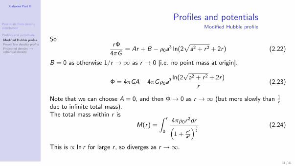
3 ln(2√a2 + r2 + 2r) (2.22)

B = 0 as otherwise 1/r →∞ as r → 0 [i.e. no point mass at origin].

Φ = 4πGA− 4πGρ0a3 ln(2

√a2 + r2 + 2r)

r(2.23)

Note that we can choose A = 0, and then Φ→ 0 as r →∞ (but more slowly than 1r

due to infinite total mass).The total mass within r is

M(r) =

∫ r

0

4πρ0r2dr(

1 + r2

a2

) 32

(2.24)

This is ∝ ln r for large r , so diverges as r →∞.

31 / 41

Galaxies Part II






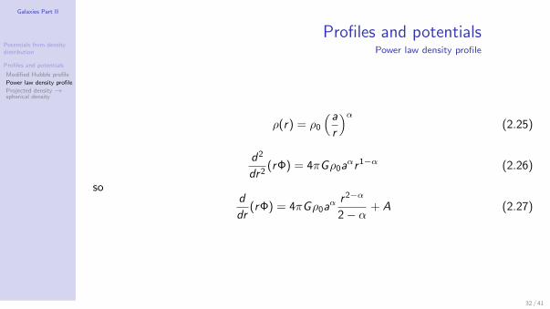
Profiles and potentialsPower law density profile

ρ(r) = ρ0

(ar

)α(2.25)

d2

dr2(rΦ) = 4πGρ0a

αr1−α (2.26)

sod

dr(rΦ) = 4πGρ0a

α r2−α

2− α+ A (2.27)

32 / 41

Galaxies Part II







rΦ = 4πGρ0aα r3−α

(2− α)(3− α)+ Ar + B (2.28)

or

Φ = − 4πGρ0aαr2−α

(3− α)(α− 2)+ A +

B

r(2.29)

A = 0 by setting zero, and B = 0 because no point mass at centre as usual.

33 / 41

Galaxies Part II







��

��Φ = − 4πGρ0a

αr2−α

(3−α)(α−2)

�� ρ(r) = ρ0

(ar

)αNotes:(1) α < 3 to get M(r) finite at the origin (determine

∫4πGρr2dr near origin).

(2) Φ→ 0 at ∞ if α > 2,⇒ 2 < α < 3

α = 2 gives spiral rotation curves (flat), from v2c /r = dΦ

dr (= −fr )⇒ v2c ∝ r2−α.

[Circular motion ⇒ r & r = 0, so r − r φ2 = − dΦdr becomes, with vc = r φ,

v2c

r = − dΦdr .

Then substituting Φ from equation (2.29) gives v2c ∝ r2−α.]

α = 3 gives elliptical galaxy profiles (mod. Hubble profile)but all these models have infinite mass, since M(r) diverges at large r

34 / 41

Galaxies Part II






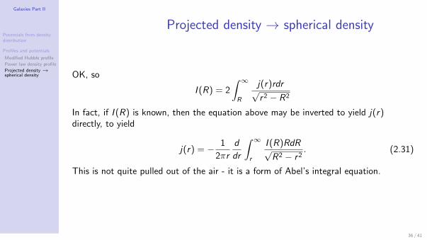
Projected density → spherical densityWhat we have done so far is to guess a luminosity density j(r) (which we assume isproportional to the matter density ρ(r)) and formed the projected surface brightnessI (R) using the relation

I (R) = 2

∫ ∞R

j(r)rdr√r2 − R2

(2.30)

and then check that I (R) is a reasonable approximation to what is seen for our guesseddensity distribution.

r2 = x2 + R2

dx =rdr√

r2 − R2

35 / 41

Galaxies Part II






Projected density → spherical density

OK, so

I (R) = 2

∫ ∞R

j(r)rdr√r2 − R2

In fact, if I (R) is known, then the equation above may be inverted to yield j(r)directly, to yield

j(r) = − 1

2πr

d

dr

∫ ∞r

I (R)RdR√R2 − r2

. (2.31)

This is not quite pulled out of the air - it is a form of Abel’s integral equation.

36 / 41

Galaxies Part II






Projected density → spherical densityWe can simplify the form a bit if we set t = R2 and x = r2, and then we have

I (t) =

∫ ∞t

j(x)dx

(x − t)12

and then the inverse relation quoted becomes

j(y) = − 1

π

d

dy

∫ ∞y

I (t)dt

(t − y)12

If we look just at the RHS, and call it h(y) for the moment, this is

h(y) = − 1

π

d

dy

∫ ∞y

dt

(t − y)12

∫ ∞t

j(x)dx

(x − t)12

.

or

h(y) = − 1

π

d

dy

∫ ∞t=y

∫ ∞x=t

dtj(x)dx

(t − y)12 (x − t)

12

37 / 41

Galaxies Part II







We now switch the order of the integration, remembering when doing so to change thelimits of the integration so that we are integrating over the same area in the(x , t)-plane.

h(y) = − 1

π

d

dy

∫ ∞y

j(x)dx

∫ x

y

dt

(t − y)12 (x − t)

12

The integral ∫ x

y

dt

(t − y)12 (x − t)

12

= π

and so what we called h(y) is then seen to be equal to j(y). So the result follows.

38 / 41

Galaxies Part II







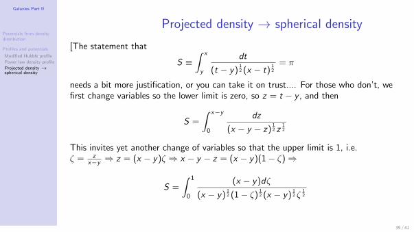
[The statement that

S ≡∫ x

y

dt

(t − y)12 (x − t)

12

= π

needs a bit more justification, or you can take it on trust.... For those who don’t, wefirst change variables so the lower limit is zero, so z = t − y , and then

S =

∫ x−y

0

dz

(x − y − z)12 z

12

This invites yet another change of variables so that the upper limit is 1, i.e.ζ = z

x−y ⇒ z = (x − y)ζ ⇒ x − y − z = (x − y)(1− ζ)⇒

S =

∫ 1

0

(x − y)dζ

(x − y)12 (1− ζ)

12 (x − y)

12 ζ

12

39 / 41

Galaxies Part II






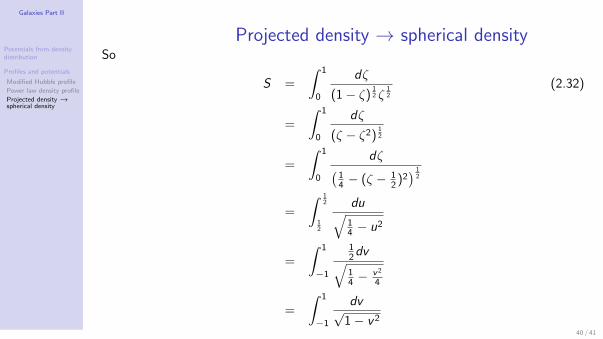
Projected density → spherical densitySo

S =

∫ 1

0

dζ

(1− ζ)12 ζ

12

(2.32)

=

∫ 1

0

dζ

(ζ − ζ2)12

=

∫ 1

0

dζ(14 − (ζ − 1

2 )2) 1

2

=

∫ 12

12

du√14 − u2

=

∫ 1

−1

12dv√14 −

v2

4

=

∫ 1

−1

dv√1− v2

40 / 41

Galaxies Part II







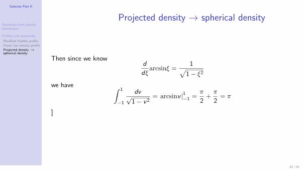
Then since we knowd

dξarcsinξ =

1√1− ξ2

we have ∫ 1

−1

dv√1− v2

= arcsinv |1−1 =π

2+π

2= π

]

41 / 41

Documents

Stellar Dynamics and Structure of Galaxies - …vasily/Lectures/SDSG/sdsg_2_poisson.pdf · Galaxies Part II Potentials from density distribution Poisson’s Equation Gauss’s Theorem