Stellar Atmospheres Theory� An Introduction

I� Hubeny

Universities Space Research Association� NASA Goddard Space Flight Center�Code ���� Greenbelt� MD ������ USA

� Fundamental Concepts

��� What is a Stellar Atmosphere� and Why Do We Study It�

By the term stellar atmosphere we understand any medium connected phys�ically to a star from which the photons escape to the surrounding space� Inother words� it is a region where the radiation� observable by a distant ob�server� originates� Since in the vast majority of cases the radiation is the onlyinformation about a distant astronomical object we have �exceptions beinga direct detection of solar wind particles� neutrinos from the Sun and SN����a� or gravitational waves�� all the information we gather about stars isderived from analysis of their radiation�

It is therefore of considerable importance to develop reliable methodswhich are able to decode the information about a star contained in its spec�trum with condence� Having understood the physics of the problem andbeing able to carry out detailed numerical simulations will enable us to con�struct theoretical models of a stellar atmosphere and predict a stellar spec�trum� This has important applications in other branches of astrophysics� suchas i� derived stellar parameters can be used to verify predictions of the stel�lar evolution theory ii� models provide ionizing �uxes for the interstellarmedium and nebular models iii� predicted stellar spectra are basic blocks forpopulation syntheses of stellar clusters� starburst regions� and whole galaxies�Moreover� very hot and massive stars have special signicance� They are verybright� and therefore may be studied spectroscopically as individual objectsin distant galaxies� Reliable model atmospheres for these stars may thereforeyield invaluable independent information about distant galaxies� like chemicalcomposition� and� possibly� reliable distances�

This alone would easily substantiate viewing the stellar atmosphere theoryas an independent� and very important� branch of modern astrophysics� Yet�in the global astrophysical context� there is another� and equally important�contribution of the stellar atmospheres theory� Stellar atmospheres are thebest studied example of a medium where radiation is not only a probe ofthe physical state� but is in fact an important constituent� In other words�radiation in fact determines the structure of the medium� yet the medium isprobed only by this radiation�

� I� Hubeny

Unlike laboratory physics� where one can change a setup of the experimentin order to examine various aspects of the studied structures separately� we donot have this luxury in astrophysics� we are stuck with the observed spectrumso we should better make a good use of it� This is exactly what the stellaratmosphere theory is doing for almost a century now� Consequently� it isdeveloped to such an extent that it provides an excellent methodologicalguide for other situations where the radiation has the dual role of a probeand a constituent� Examples of such astronomical objects are the interstellarmedium� H II regions� and� in particular� accretion disks�

There has been a signicant progress in the eld of stellar atmospheresachieved in recent years� The progress was motivated by an unprecedentedincrease of quality of ground� and space�based observations� and by develop�ment of extremely fast and e cient numerical methods� However� despite ofthis progress� the stellar atmospheres theory is still far from being su cientlydeveloped� It is a mature eld� yet it is now reaching qualitatively new levelsof sophistication� In short� it is a eld worth pursuing� o�ering as a reward asignicant contribution to our knowledge about the Universe�

The main goal of this lecture is to provide a gentle introduction to thebasic concepts needed to understand the fundamental physics of stellar atmo�spheres� as well as the leading principles behind recent developments� Partic�ular emphasis will be devoted to the classical plane�parallel atmospheres inhydrostatic and radiative equilibrium� Topics which concentrate specicallyon non�static phenomena �stellar winds�� and on departures from radiativeequilibrium �stellar chromospheres and coronae�� are covered in other lecturesof this volume�

There is no textbook that would fully cover the topics discussed in this lec�ture� The fundamental textbook of the eld� Mihalas ������� is still a highlyrecommended text� although it does not cover important recent develop�ments� like for instance the ALI method� The third edition of the book is nowin preparation� but it will take a couple of years before it is available� There isa recent textbook by Rutten ������� distributed electronically� which coversboth the basic concepts as well as some of the modern development� and ishighly recommended to the beginner in the eld� There are two books editedby Kalkofen which present a collection of reviews on various mathematicaland numerical aspects of radiative transfer �Kalkofen ���� ������ A goodtextbook that covers both the theoretical and observational aspects of thestellar atmospheres is that by Gray ������� Other related textbooks includeRybicki and Lightman ������� Shu ������� and an elementary�level textbookby B�ohm�Vitense ������� An old but excellent textbook on radiative trans�fer is Je�eries ������� Besides these books� there are several excellent reviewpapers covering various topics �e�g� Kudritzki ���� Kudritzki and Hummer������ and several conference proceedings which contain many interestingpapers on the stellar atmospheres theory � Properties of Hot Luminous Stars�Garmany ����� Stellar Atmospheres� Beyond Classical Models �Crivellari�

Stellar Atmospheres Theory� An Introduction

Hubeny� and Hummer ����� The Atmospheres of Early�Type Stars �Heberand Je�ery ����� and Hydrogen�Decient Stars �Je�ery and Heber �����to name just few of the most important ones�

��� Basic Structural Equations

A stellar atmosphere is generally a plasma composed of many kinds of parti�cles� namely atoms� ions� free electrons� molecules� or even dust grains� andphotons� Typical values of temperature range from ��� K �or even less inthe coolest stars� to a few times ��� K in the hottest stars �temperature iseven higher� ��� � ��� K� in stellar coronae�� Likewise� the total particle den�sity ranges from� say� ��� to ���� cm��� Under such conditions� the naturalstarting point for the physical description is the kinetic theory�

We start with very general equations� in order to emphasize a close con�nection of the stellar atmospheres theory and other branches of physics� Wewill then simplify these equations to the form which is used in most textbooks�

Specically� the most general quantity which describes the system is thedistribution function fi�r�p� t�� which has the meaning that fi�r�p� t�drdpis the number of particles of kind i in an elementary volume of the phasespace at position r� momentum p� and at time t� The equation which de�scribes a development of the distribution function is the well�known kinetic�or Boltzmann� equation� written as

�fi�t

� �u � r� fi � �F � rp� fi �

�DfiDt

�coll

� ���

where r and rp are the usual nabla di�erential operators with respect toposition and momentum components� respectively u is the particle velocity�and F is the external force� The term �Df�Dt�coll is the so�called collisionalterm� which describes creations and destructions of particles of type i withthe position �r� r� dr� and momentum �p�p� dp��

The kinetic equation provides a full description of the system� However�the number of unknowns is enormous� It should be realized that the individualparticles are� in general� not just the atoms and ions� but in fact all theindividual excitation states of atoms� ions� or molecules� According to thestandard procedure� one simplies the system by constructing equations forthe moments of the distribution function� i�e� the integrals over momentumweighted by various powers of p� I shall present only the nal equations thereader is referred to any standard textbook of the kinetic theory for a detailedderivation and an extensive discussion�

The resulting set of equations are the well�known hydrodynamic equa�tions� namely the continuity equation�

��

�t�r � ��v� � � � ���

I� Hubeny

the momentum equation�

���v�

�t�r � ��vv� � �rP � f � ���

and the energy balance equation�

�

�t

��

��v� � ��

��r�

���

��v� � ��� P

�v

�� f �v�r��Frad � Fcon� � ���

Here� v is the macroscopic velocity� � the total mass density� P the pressure�f the external force� � the internal energy� Frad the radiation �ux� and Fcon

the conductive �ux� Equations ��� � ��� represent moment equations of thekinetic equation� ���� summed over all kinds of particles�

We may also write a zeroth�order moment equation for the individualkinds of particles� i�e� the conservation equation for particles of type i�

�ni�t

�r � �niv� �

�DniDt

�coll

� ���

where ni is the number density �or the occupation number� or population� ofparticles of type i� One may also write momentum and energy balance equa�tions for the individual particles if needed �e�g� if di�erent kinds of particleshave di�erent macroscopic velocities�� We will not consider these situationshere�

The moment equations are still quite general� An application of thoseequations is discussed in other papers of this volume� Here� I will present afurther signicant simplication of the system� which applies for the case of astationary �i�e� ���t � ��� and moreover static �v � �� medium� Finally� wewill consider a ��D situation� i�e� all quantities depend on the z�coordinateonly� �

DniDt

�coll

� � � ���

rP � f �� dP

dz� ��g � ���

rFrad � � �� Frad � const � �T �e� � ���

where � is the Stefan�Boltzmann constant� and Te� is the so�called e�ectivetemperature� The rst equation is called the statistical equilibrium equation�the second one the hydrostatic equilibrium equation� while the last one� ex�pressing the fact that the only mechanism that transports energy is radiation�is called the radiative equilibrium equation� �Notice that the conductive �uxwas neglected here� which is a common approximation in the stellar atmo�spheres theory� However� this approximation breaks down� for instance� inthe solar transition region��

What about convection� which we know may contribute signicantly tothe energy balance in certain types of stellar atmospheres� Convection is a

Stellar Atmospheres Theory� An Introduction �

transport of energy by rising and falling bubbles of material with properties�e�g� temperature� di�erent from the ambient medium� It is therefore� by itsvery nature� a non�stationary and non�homogeneous phenomenon� Puttingv � � and assuming a ��D medium means� strictly speaking� that convectionis a priori neglected� However� there are descriptions� like the mixing�lengththeory �see any standard textbook� like Mihalas ������ that simplify theproblem and cast it in the form of ��D stationary equation� viz�

Frad � Fconv � �T �e� � ���

where the convective �ux Fconv is a specied function of basic state parame�ters �temperature� density� etc��

So far� we have specied the kinetic equation for particles� The samemay be done for photons� Since� as explained above� photons have a specialsignicance in stellar atmospheres� we will consider the kinetic equation forphotons � the so�called radiative transfer equation � in the Sect� ��

��� LTE versus non�LTE

It is well known from statistical physics that a description of material prop�erties is greatly simplied if the thermodynamic equilibrium �TE� holds� Inthis state� the particle velocity distributions as well as the distributions ofatoms over excitation and ionization states are specied uniquely by twothermodynamic variables� In the stellar atmospheres context� these variablesare usually chosen to be the absolute temperature T � and the total particlenumber density� N � or the electron number density� ne� From the very natureof a stellar atmosphere it is clear that it cannot be in thermodynamic equilib�rium � we see a star� therefore we know that photons must be escaping� Sincephotons carry a signicant momentum and energy� the elementary fact ofphoton escape has to give rise of signicant gradients of the state parametersin the stellar outer layers�

However� even if the assumption of TE cannot be applied for a stellaratmosphere� we may still use the concept of local thermodynamic equilibrium� LTE� This assumption asserts that we may employ the standard thermody�namic relations not globally for the whole atmosphere� but locally� for localvalues of T �r� and N �r� or ne�r�� despite the gradients that exist in the at�mosphere� This assumption simplies the problem enormously� for it impliesthat all the particle distribution functions may be evaluated locally� with�out reference to the physical ensemble in which the given material is found�Notice that the equilibrium values of distribution functions are assigned tomassive particles the radiation eld is allowed to depart from its equilibrium�Planckian � ����� distribution function�

Specically� LTE is characterized by the following three distributions�� Maxwellian velocity distribution of particles

f�v�dv � �m���kT ���� exp��mv���kT � dv � ����

� I� Hubeny

where m is the particle mass� and k the Boltzmann constant�� Boltzmann excitation equation�

�nj�ni� � �gj�gi� exp ���Ej �Ei��kT � � ����

where gi is the statistical weight of level i� and Ei the level energy� measuredfrom the ground state�

� Saha ionization equation�

NI

NI��� ne

UIUI��

C T���� exp��I�kT � � ����

where NI is the total number density of ionization stage I� U is the partitionfunction� dened by U �

P�

� gi exp��Ei�kT � �I is the ionization potentialof ion I� and C � �h����mk���� is a constant �� ���������� in cgs units�� Itshould be stressed that in the astrophysical LTE description� the same tem�perature T applies to all kinds of particles� and to all kinds of distributions����� � �����

Equations ���� � ���� dene the state of LTE from the macroscopic pointof view� Microscopically� LTE holds if all atomic processes are in detailed bal�

ance� i�e� if the number of processes A� B is exactly balanced by the numberof inverse processes B � A� By A and B we mean any particle states be�tween which there exists a physically reasonable transition� For instance� Ais an atom in an excited state i� and B the same atom in another state j�either of the same ion as i� in which case the process is an excitation�de�excitation or of the higher or lower ion� in which case the term is an ioniza�tion�recombination�� An illuminating discussion is presented in the textbookby Oxenius �������

In contrast� by the term non�LTE �or NLTE� we understand any statethat departs from LTE� In practice� one usually means that populations ofsome selected energy levels of some selected atoms�ions are allowed to departfrom their LTE value� while velocity distributions of all particles are assumedto be Maxwellian� ����� moreover with the same kinetic temperature� T �

One of the big issues of modern stellar atmospheres theory is whether� andif so to what extent� should departures from LTE be accounted for in numeri�cal modeling� This question will be discussed in more detail later on �Sects� ����� Generally� to understand why and where we may expect departures fromLTE� let us turn to the microscopic denition of LTE� It is clear that LTEbreaks down if the detailed balance in at least one transition A � B breaksdown� We distinguish the collisional transitions �arising due to interactionsbetween two or more massive particles�� and radiative transitions �interac�tions involving particles and photons�� Under stellar atmospheric conditions�collisions between massive particles tend to maintain the local equilibrium�since velocities are Maxwellian�� Therefore� the validity of LTE hinges onwhether the radiative transitions are in detailed balance or not�

Stellar Atmospheres Theory� An Introduction �

Again� the fact that the radiation escapes from a star implies that LTEshould eventually break down at a certain point in the atmosphere� Essen�tially� this is because detailed balance in radiative transitions generally breaksdown at a certain point near the surface� Since photons escape �and moreso from the uppermost layers�� there must be a lack of them there� Conse�quently� the number of photoexcitations �or any atomic transition induced byabsorbing a photon� is less than a number of inverse processs� spontaneousde�excitations �we neglect here� for simplicity� stimulated emission��

These considerations explain that we may expect departures from LTEif the following two conditions are met� i� radiative rates in some importantatomic transition dominate over the collisional rates and ii� radiation is notin equilibrium� i�e� the intensity does not have the Planckian distribution�Later� we will show how these conditions are satised in di�erent stellartypes� However� some general features can be seen immediately� Collisionalrates are proportional to the particle density it is therefore clear that forhigh densities the departures from LTE tend to be small� Likewise� deepin the atmosphere� photons do not escape� and so the intensity is close tothe equilibrium value� Departures from LTE are therefore small� even if theradiative rates dominate over the collisional rates�

� Radiative Transfer Equation

As explained above� radiation plays a somewhat privileged role in the stellaratmospheres theory� This is the reason why we consider the radiative transferequation separately from equations describing the material properties� Thedominant role of radiation is also re�ected in the terminology � the wholestellar atmosphere problem is sometimes referred to as a solving the radiative

transfer equation with constraints� i�e� viewing all the material equations asmere �constraints��

As discussed in the preceding section� one may view the radiative transferequation as a kinetic equation for photons� In the astronomical literature� itis customary to start with a phenomenological derivation of the radiativetransfer equation� and to show later that this equation is in fact equivalentto the kinetic equation�

It should be realized� however� that when viewing radiation as an ensem�ble of mutually non�interacting� massless particles � photons� and describingthe interaction between radiation and matter in terms of simple collisions�interactions� between photons and massive particles� the wave phenomenaconnected with radiation are in fact neglected� This is a good approximationif i� the wavelength of radiation is much smaller than the typical distancebetween massive particles and if ii� the particle positions are random� Theseconditions are well satised under the stellar atmospheric conditions� we dealwith a hot plasma� so the particle positions are indeed random� For optical�UV� and even higher�frequency radiation� the wavelengths � ���� cm�

� I� Hubeny

are indeed smaller that typical interparticle distances� For infrared and radiowavelengths� some wave phenomena �e�g� refraction� may actually play a rolein the radiative transfer�

In the following� we will adhere to the photon picture� and neglect allthe wave phenomena� A somewhat special case is the polarization of radia�tion� Polarization will also be neglected here� i�e� we assume an unpolarizedradiation� We will see in other lectures �e�g�� Bjorkman� this volume�� thatpolarization of radiation may actually play an important diagnostic role incertains stellar atmospheric structures �as an indicator of asymmetries ofthe medium�� It is possible to extend the usual formalism of the transferequation to account for polarization� by introducing a vector quantity �theso�called Stokes vector� instead of scalar intensity of radiation� and to writedown the transfer equation in the vector form� We will not consider this casehere the interested reader is referred to standard textbooks � Chandrasekhar������ or recently Sten�o ������ or excellent review articles �several papersin Kalkofen ������

��� Intensity of Radiation and Related Quantities

We start with phenomenological denitions� The speci�c intensity� I�r�n� �� t��of radiation at position r� traveling in direction n� with frequency �� at timet is dened such that the energy transported by radiation in the frequencyrange ��� � � d��� across an elementary area dS� into a solid angle d� in atime interval dt is

dE � I�r�n� �� t� dS cos d� d� dt � ����

where is the angle between n and the normal to the surface dS �i�e�dS cos � n � dS�� The dimension of I is erg cm�� sec�� hz�� sr��� Thespecic intensity provides a complete description of the unpolarized radia�tion eld from the macroscopic point of view�

As pointed out above� there is a close connection between the specicintensity and the photon distribution function� f � The latter is dened suchthat f�r�n� �� t� d� d� is the number of photons per unit volume at locationr and time t� with frequencies in the range ��� � � d��� propagating withvelocity c in direction n� The number of photons crossing an element dS intime dt is f�c � dt��n � dS��d� d��� The energy of those photons is the sameexpression multiplied by h�� h being the Planck constant� Comparing this tothe denition of the specic intensity� we obtain the desired relation betweenthe specic intensity and the distribution function�

I � �ch�� f � ����

This relation makes it easy to understand the following expressions� Anal�ogously as for massive particles� one denes various moments of the distribu�tion function � i�e� the specic intensity in this case � which have a meaningof the energy density� �ux� and the stress tensor�

Stellar Atmospheres Theory� An Introduction �

From the denition of the distribution function� it is clear that the en�

ergy density of radiation is given by �dropping an explicit indication of thedependence on frequency� etc��

E �

I�h��f d� � ���c�

II d� � ����

because f is the number of photons in an elementary volume� and h� theenergy of each we have to integrate over all solid angles� Similarly� the energy�ux of radiation is given by

F �

I�h�� � �cn� f d� �

In I d� � ����

because cn is the vector velocity�The radiation stress tensor is dened by

P �

I�h��nnf d� � ���c�

Inn I d� � ����

Finally� we mention that the photon momentum density �recall that the mo�mentum of an individual photon is �h��c�n� is given by

G �

I�h��c�n f d� � ���c��F � ����

i�e�� it is proportional to the radiation �ux�

��� Absorption and Emission Coe�cient

The radiative transfer equation describes the changes of the radiation elddue to its interaction with matter� To describe this interaction� one rstintroduces several phenomenological quantities�

Absorption coe�cient describes the removal of energy from the radiationeld by matter� It is dened in such a way that an element of material� ofcross�section dS and length ds� removes from a beam of specic intensity I�incident normal to dS into a solid angle d��� an amout of energy

dE � ��r�n� �� t� I�r�n� �� t� dS d� d� dt � ����

The dimension of � is cm��� thus ��� has a dimension of length� and itmeasures a characteristic distance a photon can travel before it is absorbedin other words� the photon mean free path�

Emission coe�cient describes the energy released by the material in the formof radiation� Analogously� it is dened such as an elementary volume of ma�terial� of cross�section dS and length ds� releases �into a solid angle d�� indirection n� within a frequency band d�� an amout of energy

dE � ��r�n� �� t� dS d� d� dt � ����

�� I� Hubeny

The dimension of � is erg cm�� hz�� sec�� sr���The absorption and emission coe cients are dened per unit length� Some�

times� one denes the coe cients per unit mass� which are given by expres�sions ���� and ���� divided by the mass density� ��

The above coe cients are dened phenomenologically� To be able to writedown actual expressions for them� we have to go to microscopic physics� Inother words� we have to describe all contributions from microscopic processesthat give rise to an absorption or emission of photons with specied proper�ties� Detailed expressions will be considered later on �Sects� ���� ����� Here�we will discuss some general points�

i� Sometimes� one distinguishes two types of absorption� a �true absorp�tion�� and a �scattering�� In the true absorption �also called �thermal absorp�tion�� process� a photon is removed from the incident beam and is destroyedwhile in the scattering process a photon is rst removed from the beam� butis immediately re�emitted in a di�erent direction and with �slightly� di�erentfrequency� This distinction is re�ected in a notation�

��r�n� �� t� � ��r�n� �� t� � ��r�n� �� t� � ����

where the rst term on the right hand side� �� refers to the true absorption�while the second term� �� to the scattering� However� I stress that this distinc�tion does not really have to do much with the absorption process � � describesa removal of photon from the beam and does not have to care about whathappens next� The distinction between the true absorption and scatteringactually enters rather the proper formulation of the emission coe cient�

ii� It is known from the quantum theory of radiation that there are threetypes of elementary processes that give rise to an absorption or emission ofa photon� �� induced absorption � an absorption of a photon accompaniedby a transition of an atom�ion to a higher energy state� �� spontaneousemission � an emission of a photon accompanied by a spontaneous transitionof an atom�ion to a lower energy state� and �� stimulated emission � aninteraction of an atom�ion with a photon accompanied by an emission ofanother photon with identical properties� In the astrophysical formalism� thestimulated emission is usually treated as negative absorption�

iii� In thermodynamic equilibrium� the microscopic detailed balance holds�and therefore the radiation energy absorbed in an elementary volume in anelementary frequency interval is exactly balanced by the energy emitted in thesame volume and in the same frequency range� From the denition expressionsfor the absorption and emission coe cients� ���� and ����� it follows that inthe equilibrium state� � I � �� Moreover� we know that in thermodynamicequilibrium the radiation intensity is equal to the Planck function� I � B�where

B��� T � ��h��

c��

exp�h��kT �� �� ����

We are then left with an interesting relation that in thermodynamic equilib�rium� ��� � B� which is called Kirchho��s law�

Stellar Atmospheres Theory� An Introduction ��

��� Phenomenological Derivation of the Transfer Equation

Having dened the basic phenomenological coe cients which describe theinteraction of radiation and matter� a heuristic derivation of the radiativetransfer equation is straightforward� We express a conservation of the totalphoton energy when a radiation beam passes through an elementary volumeof matter of cross�section dS �perpendicular to the direction of propagation�and length ds �measured along the direction of propagation�� Taking intoaccount denitions of the specic intensity� ����� and the absorption andemission coe cients� ���� and ����� we obtain

�I�r� �r�n� �� t��t�� I�r�n� �� t�� dS d� d� dt �

���r�n� �� t�� ��r�n� �� t�I�r�n� �� t�� ds dS d� d� dt � ����

which expresses the fact that the di�erence between specic intensities beforeand after passing through the elementary volume of pathlength ds is equalto the di�erence of the energy emitted and absorbed in the volume� Thedi�erence of intensities on the left hand side may be expressed as

di� I ��I

�sds�

�I

�tdt �

��I

�s�

�

c

�I

�t

�ds � ����

Finally� �I��s may be written as n � r� so we arrive at

��

c

�

�t� n � r

�I�r�n� �� t� � ��r�n� �� t�� ��r�n� �� t� I�r�n� �� t� � ����

This is the general form of the radiative transfer equation� Let us now considertwo important special cases�

�� for a one�dimensional planar atmosphere� nz � �dz�ds� � cos � ��where is the angle between direction of propagation of radiation� n� and thenormal to the surface� Further� let us assume a time�independent situation����t � �� so we obtain

�dI��� �� z�

dz� ���� �� z�� I��� �� z����� �� z� � ����

where the intensity of radiation is now only a function of the geometricalcoordinate z� frequency �� and the directional cosine ��

�� in spherical coordinates� the derivative along the ray� ���s is given by���s � �����r� � �� � ����r������� and the radiative transfer equation ina spherically symmetric medium is written as

��I��� �� r�

�r�

�� ��

r

�I��� �� r�

��� ���� �� r�� I��� �� r����� �� r� � ����

�� I� Hubeny

��� Optical Depth and the Source Function

Let us start with a simple ��D transfer equation� written as

�dI�dz

� �� � ��I� � ����

where we drop an explicit indication of the dependence of I� �� and � onthe geometrical distance z and angle �� and write� as is customary in theastrophysical literature� the frequency � as a subscript� We divide the transferequation by ��� and obtain a very simple and advantageous form of thetransfer equation�

�dI�d��

� I� � S� � ����

where the elementary optical depth is dened by

d�� � ��� dz � ����

and the source function is dened by

S� � ����

� ����

The absorption and emission coe cient are local quantities� therefore thedenition of the source function� ����� applies for all geometries� The opticaldepth depends on the geometry in case of a ��D transfer� the most naturaldenition is the optical depth along the ray� dened by

d� � ��r�n� �� ds � ����

where ds is the elementary pathlength in the direction n� In the case ofa plane�parallel atmosphere� the relation between the optical depth in thedirection � �which we denote here as ����� and the �normal�direction� ��dened by ����� is

d��� � d���� � ����

What is the physical meaning of the optical depth and of the source func�tion� The meaning of the optical depth is straightforward� In the absenceof emissions� the transfer equation is simply dI�d� � I� and the solutionis I�� � � I�� � �� � exp���� �� i�e� the optical depth is the e�folding dis�tance for attenuation of the specic intensity due to absorption� In otherwords� the probability that a photon will travel an optical distance � is sim�ply p�� � � exp��� �� Since the absorption coe cient �e�g� in spectral lines�may be a sharply varying function of frequency� the �monochromatic� opticaldepth may also vary signicantly with frequency� Sometimes one denes var�ious frequency�independent optical depths� like those corresponding to theaveraged absorption coe cient� either over the whole spectrum �a typical ex�ample being the Rosseland optical depth � see Sect� ����� or over a spectralline �see Sect� �����

Stellar Atmospheres Theory� An Introduction �

The meaning of the source function can also be easily understood� Let uswrite the number of photons emitted in an elementary volume �dened by anelementary area dS and an elementary path ds�� to all directions� From thedenition of the emission coe cient it follows that �assuming an isotropicemission for simplicity� Nem � � ds ����h�� d� dt dS� where the factor ��comes from an integration over all solid angles� and h� transforms energy�from the original denition of the emission coe cient� to the number ofphotons� Using the denition of the optical depth and the source function�we may rewrite the factor � ds as � ds � ������ ds � S�� �d� � Consequently�the number of emitted photons is

Nem � S�� �d���

h�d� dt dS � ����

In other words� the source function is proportional to the number of photons

emitted per unit optical depth interval�For completeness� we mention that the number of photons absorbed per

unit optical depth interval �from all solid angles� is analogously given by

Nabs � J�� �d���

h�d� dt dS � ����

which directly follows from ���� J being the mean intensity of radiation�dened by �����

�� Elementary Solutions

In this section� we consider the simplest solutions of the ��D plane�paralleltransfer equation� For notational simplicity� we drop subscript � indicatingthe frequency dependence�

a� No absorption� no emission� i�e� � � � � �� The transfer equation readsdI�dz � �� which has a trivial solution

I � const � ����

This expresses the obvious fact that in the absence of any interaction withthe medium� the radiation intensity remains constant�

b� No absorption� only emission� i�e� � � �� but � � �� The solution issimply

I�z� �� � I��� �� �

Z z

��z��dz��� � ����

This equation is often used for describing an outcoming radiation from anoptically thin radiating slab� like for instance a forbidden line radiation fromplanetary nebulae� or a radiation from the solar transition region and�orcorona�

� I� Hubeny

c� No emission� only absorption� i�e� � � �� � � �� The transfer equationnow reads � dI�d� � I� and the solution is simply

I��� �� � I��� �� exp������ � ����

d� Absorption and emission� We will now write a general formal solution ofthe transfer equation� i�e� for the case where both� absorption and emission�coe cients are di�erent from zero� � � �� � � �� The solution is called�formal� because it is assumed here that both � and � are speci�ed functionsof position and frequency� As we shall see later on� both coe cients maydepend on the radiation eld� so that in actual problems they may not begiven a priori� without previously solving the general transfer problem� Theformal solution reads

I���� �� � I���� �� exp������ �������

Z ��

��

S�t� exp���t� ������ dt�� � ����

e� Semi�in�nite atmosphere� A special case of the formal solution ���� foremergent radiation �i�e� �� � �� from a semi�innite atmosphere ��� � ��reads

I��� �� �

Z �

S�t� exp��t��� dt�� � ����

This equation shows that the specic intensity in a semi�innite atmosphereis in fact a Laplace transform of the source function�

f� Semi�in�nite atmosphere with a linear source function� Another specialcase of the general formal solution ���� is a emergent intensity from a semi�innite atmosphere� with a source function being a linear function of opticaldepth� S�� � � a� b� � It is given by

I��� �� � a� b� � S�� ��� � ����

This important expression is called the Eddington�Barbier relation� It showsthat the emergent intensity� for instance in the normal direction �� � �� isgiven by the value of the source function at the optical depth of unity� Thevalues of emergent intensity for all angles � between � and � then map thevalues of the source function between optical depths � and �� Although inreality the source function does not have to be a linear function of opticaldepth� it can usually be well approximated by it in the vicinity of � � ��Consequently� the Eddington�Barbier relation� ����� usually provides a goodestimate of the emergent intensity�

g� Finite homogeneous slab� Finally� an expression for an emergent radia�tion ��� � �� from a nite ��� � T �� and homogeneous slab �i�e� S�t� � Sis constant�� in the normal direction �� � ��� reads

I��� �� � S � ��� e�T�� ����

Stellar Atmospheres Theory� An Introduction ��

In the special case T � �� ���� becomes I��� �� � S� while for T � �� weobtain I��� �� � S � T � Both limiting expressions have a simple physical ex�planation� As we have shown above� the source function expresses a numberof photons �or radiative energy� emitted per unit optical depth� In the opti�cally thin case �T � ��� there is little absorption� so practically all createdphotons escape from the medium� Since the actual optical depth is T � thetotal emergent intensity is S �T � In the optical thick case� we may roughly saythat the photons created deeper than � � � are very likely absorbed� so theonly photons which contribute to the emergent intensity are those emittedat optical depths � �� Consequently� the emergent intensity is S � �� i�e� S�regardless of the actual optical thickness of the slab�

�� Moments of the Transfer Equation

Analogously to the case of massive particles� we may dene various momentsof the photon distribution function� i�e� the specic intensity� By appropri�ately integrating the kinetic �i�e� transfer� equation we obtain relations be�tween these moments� As was discussed in Sect� ����� the rst three momentsare the photon energy density� radiation �ux� and the radiation stress tensor�Written synoptically� �see� e�g the textbook by Shu ������ we may write�

� cE�

F�cP�

�A �

I �� �

nnn

�A I�d� � ����

Consequently� the moment equations are obtained by multiplying the transferequation ���� by �� n� etc�� and integrating over all solid angles� The rst twomoment equations read

�E�

�t�r �F� � �� � �� cE� � ����

�

c

�F��t

� cr �P� � ��� F� � ����

Both these equations have the general structure of the moment equation ofthe kinetic equation� namely

���t�density of quantity� � �gradient of its �ux� � �sources � sinks� � ����

In the astrophysical literature� one usually introduces moments as angle�averaged� rather than angle�integrated quantities� The rst moments of theradiation intensity are usually denoted as J � H� K� We may synopticallywrite �

� J�H�

K�

�A �

�

��

�� cE�

F�cP�

�A �

�

��

I �� �

nnn

�A I�d� � ����

�� I� Hubeny

In a plane�parallel approximation� all the moments are scalar quantities�and are given by

J� ��

�

Z �

��I����d� � ����

H� ��

�

Z �

��� I����d� � ����

K� ��

�

Z �

����I����d� � ����

and the moment equations are written as

dH�

d��� J� � S� � ����

anddK�

d��� H� � ����

The system of moment equations is not closed� i�e� the equation for n�thmoment contains the �n����th moment� etc� It is therefore necessary to comeup with some kind of closure relation� In the stellar atmospheres theory� onedenes the so�called Eddington factor� fK� by

fK� � K��J� � ����

It is clear from the denition of moments that in the case of isotropic radia�tion� I���� � I� being independent of angle� the Eddington factor fK � ����Assuming the Eddington factor to be specied� one may combine the twomoment equations ���� and ���� together�

d��fK� J��

d���� J� � S� � ����

This equation is very useful� It e�ectively eliminates one independent vari�able� the angle �� from the problem� Numerically� it replaces the originaltransfer equation� which is a rst�order linear di�erential equation for thespecic intensity I��� by a second�order but still linear di�erential equationfor the mean intensity� J� � However� its simplicity is illusory� It cannot beused alone� even if the source function is given� since in general the Ed�dington factor is unknown unless the full solution of the transfer equation isknown� However� this form of the transfer equation is very useful in certainnumerical methods� as we will discuss later on� It should be realized that itcan be used to advantage only in iterative methods in which we use currentvalues of J and K to determine the current Eddington factor fK� and keepthis factor xed during the subsequent iteration step�

Stellar Atmospheres Theory� An Introduction ��

��� Lambda Operator

Let us rst write down the general formal solution of the radiative trans�fer equation for a semi�innite plane�parallel atmosphere� with no incomingradiation at the surface �� � ���

I���� � �� �

Z �

��

S� �t�e�t������ dt�� � for � � � ����

I���� � �� �

Z ��

S��t�e����t����� dt����� � for � � � ����

Recall that from the denition of the directional cosine � follows that posi�tive values of � correspond to outward directions� while negative values of �correspond to inward directions� The mean intensity of radiation is obtainedby integrating ���� and ���� over �� viz�

J����� ��

�

Z �

S��t�E��jt� �� j� dt � ����

where E� is the rst exponential integral� The general exponential integral isdened by

En�x� �Z �

�

e�xt

tndt � ����

The mean intensity may be synoptically expressed as an action of anoperator� �� on the source function�

J����� � ��� �S�t�� � ����

where the ��operator is dened by

�� �f�t�� ��

�

Z �

E��jt� � j� f�t� dt � ����

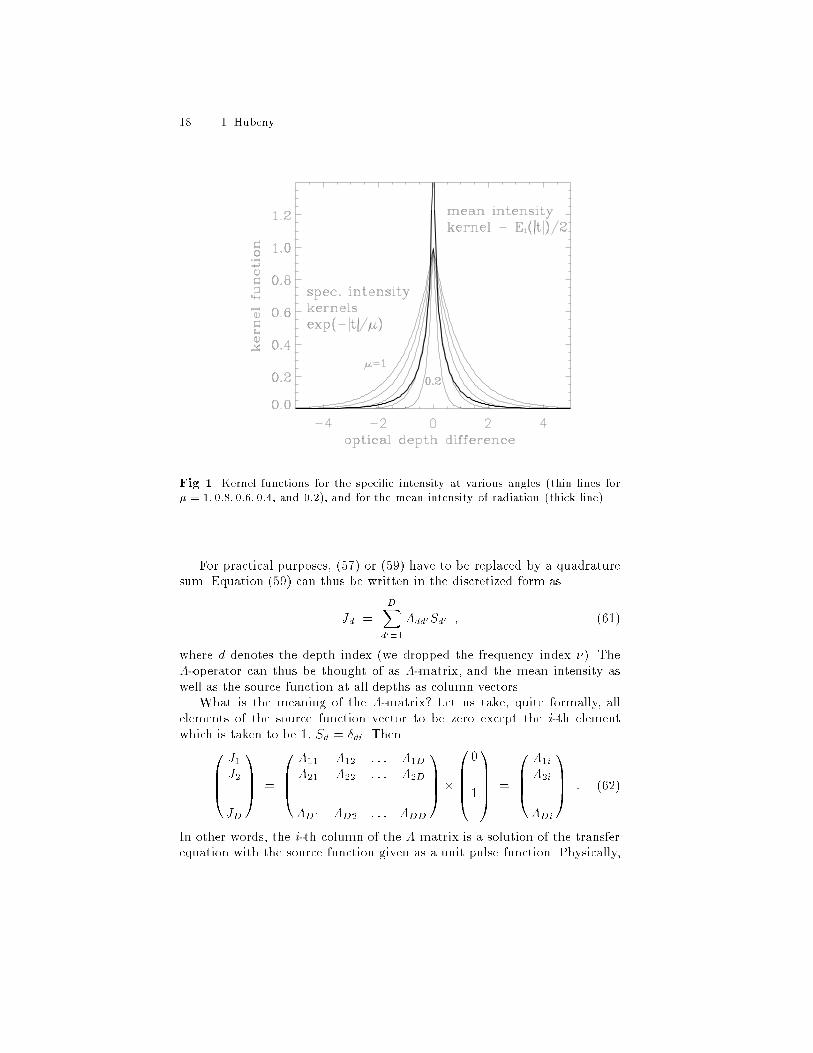
The behavior of the kernel functions corresponding to the specic inten�sity� ����� which is a simple exponential� and for the mean intensity� whichis the rst exponential integral� ����� is displayed in Fig� � The width of thekernel decreases with decreasing �� which is easily understood by realizingthat a unit optical distance for a photon traveling with a certain angle withrespect to the normal to the surface� �� corresponds to a larger optical dis�tance than for one traveling in the normal direction� because the distanceis proportional to ���� Similarly� the kernel for the specic intensity propa�gating in the normal direction �� � �� is signicantly wider than the kernelfor the mean intensity� This is simply because the mean intensity containscontribution from all angles� i�e� the corresponding kernel is an average overall ��dependent specic intensity kernels�

�� I� Hubeny

Fig� �� Kernel functions for the speci c intensity at various angles �thin lines for� � �� ���� ���� ��� and ����� and for the mean intensity of radiation �thick line�

For practical purposes� ���� or ���� have to be replaced by a quadraturesum� Equation ���� can thus be written in the discretized form as

Jd �DX

d���

�dd�Sd� � ����

where d denotes the depth index �we dropped the frequency index ��� The��operator can thus be thought of as ��matrix� and the mean intensity aswell as the source function at all depths as column vectors�

What is the meaning of the ��matrix� Let us take� quite formally� allelements of the source function vector to be zero except the i�th elementwhich is taken to be �� Sd � �di� Then�

BB�J�J����JD

�CCA �

�BB�

��� ��� � � � ��D

��� ��� � � � ��D���

���� � �

����D� �D� � � � �DD

�CCA�

�BBB�

��������

�CCCA �

�BB�

��i

��i���

�Di

�CCA � ����

In other words� the i�th column of the � matrix is a solution of the transferequation with the source function given as a unit pulse function� Physically�

Stellar Atmospheres Theory� An Introduction ��

the i�th column of � therefore describes how the pulse which originated atthe i�th depth point spreads over all depths�

��� Di usion Approximation

Deep in the atmosphere� the source function approaches the Planck function�S� � B� � because virtually no photons escape� and thus the medium ap�proaches the thermal equilibrium� Let us choose a reference optical depth��� � �� and let us expand the source function for t� �� by a Taylorexpansion�

S��t�� ��Xn�

dnB�

d�n�

�t� � ���n

n�� ����

Substituting this expression to the formal solution� ���� and ����� we obtain

I��t� � �� ��Xn�

�ndnB�

d�n�� B����� � �

dB�

d��� ��

d�B�

d���� � � � � ����

By substituting this expression into denition equations for the moments� weobtain

J����� � B����� ��

�

d�B�

d���� � � � � ����

H����� ��

�

dB�

d��� � � � � ����

K����� ��

�B����� �

�

�

d�B�

d���� � � � � ����

These equations illustrate several features of the behavior of the radiationeld at large depths� First� the mean intensity approaches the Planck func�tion� Second� the radiation eld is nearly isotropic� and the Eddington factorfK� � K��J� approaches ���� Finally� the monochromatic �ux is given as aderivative of the Planck function with respect to the optical depth� Since thePlanck function is only a function of temperature� we may express the �uxby means of the temperature gradient�

H� ��

�

dB�

d��� ��

�

�

��

dB�

dz� ��

�

�

��

dB�

dT

dT

dz� ����

Thus� at great depths the transfer problem reduces to this single equation�The name di�usion approximation comes from the similarity of this equationto other� material� di�usion equations� which are typically of the form

�ux � �di�usion coe cient� � �gradient of the relevant quantity�� ����

We may thus think of the term �������������dB��dT � as a radiative di�u�

sion coe�cient or� because of a similarity of ���� to the heat conductivityequation� as radiative conductivity�

�� I� Hubeny

By integrating over all frequencies we obtain for the total radiation �ux

in the di�usion approximation

H � ��

�

�

�

�R

dB

dT

�dT

dz� ����

where the averaged opacity is dened by

�

�R

dB

dT�

Z �

�

��

dB�

dTd� � ����

which is the well�known Rosseland mean opacity� One may dene many otheraveraged �mean� opacities by simpler expressions� but we see why the Rosse�land opacity is dened by this seemingly strange expression � it yields theexact total radiation �ux at large depths� Since the temperature in the atmo�sphere is in fact determined by the condition imposed on the total radiation�ux� the Rosseland mean opacity yields the correct temperature structure

deep in the atmosphere� It is also clear why the Rosseland opacity is themost appropriate one for the use in the stellar interior theory �de Greve�this volume�� Notice also that the integrand in the denition of Rosselandopacity contains ���� i�e� the contribution to the integral is largest for thelowest monochromatic opacities� Indeed� for those frequencies the mediumis most transparent� and therefore the monochromatic �ux is largest� Thisagain shows that the Rosseland mean opacity is the most appropriate one fordescribing the total radiation �ux�

� Radiative Transfer with Constraints� Escape

Probability

��� Two�level Atom

The simplest situation where we have a coupling of the radiative transferequation and the statistical equilibrium equation is an idealized case of atwo�level atom� Real atoms contain many energy levels� so that this approxi�mation may seem at rst sight to be grossly inadequate� However it actuallyprovides a surprisingly good description of line formation in many cases of in�terest� And� more importantly� the case of the two level atom has a signicantpedagogical value because it provides an explanation of many elementary pro�cesses that are crucial to understand NLTE line formation� In other words�a good physical understanding of line formation in a two�level atom is a pre�requisite to understanding of more complicated cases� Therefore� this modelwill be discussed here in certain detail�

Let us rst derive the expression for the source function� Figure � showsschematically the energy levels and all the elementary processes populating

Stellar Atmospheres Theory� An Introduction ��

Fig� �� Schematic representation of microscopic processes in s two�level atom

and depopulating the levels� The absorption and emission coe cients aregiven by

�� �h���

�n�B�� � n�B������� � ����

and

�� �h�o��

n�A������ � ����

where � is the line�center frequency� and B��� B�� and A�� are the Einsteincoe cients for absorption� stimulated emission� and spontaneous emission�respectively� for the radiative transitions between levels � and � n� and n�are populations �occupation numbers� of levels � and �� respectively� and ����is the absorption pro�le� The latter expresses the probability density that ifa photon is absorbed �emitted� in a line ���� it has a frequency in the range��� ��d��� The prole coe cient is thus normalized to unity�

R� ����d� � ��

We assume that there is no other absorption or emission mechanism present�It is advantageous to introduce a dimensionless frequency� x� by

x � � � ���D

� ����

��D is the Doppler width� given by ��D � ���c�vth� with the thermalvelocity vth � ��kT�m����� m being the mass of the radiating atom� In thecase of a pure Doppler prole �i�e� no intrinsic broadening of the spectral linethe only broadening is due to the thermal motion of radiators�� the absorptionprole is given by

��x� � exp��x���p� � ����

�� I� Hubeny

In a more general case� where there is an intrinsic broadening of lines de�scribed by a Lorentz prole in the atomic rest frame �the most commontypes of intrinsic broadening being the natural� Stark� and Van der Waalsbroadening � see Mihalas ����� or monograph by Griem ������ the prolefunction is given by the Voigt function�

��x� � H�a� x��p�� H�a� x� �

a

�

Z �

��

e�y�

�x� y�� � a�dy � ����

The Voigt function is a convolution of the Doppler prole �i�e� the thermalmotions� and the Lorentz prole �intrinsic broadening�� The parameter a isa damping parameter expressed in units of Doppler width� a � �������D��where � is the atomic damping parameter� For instance� for the naturalbroadening of a line originating in a two�level atom� � � A���

Opacity in the line may be written as

�x � ���x� � ����

and analogously for �x� The optical depth corresponding the the frequency�independent opacity� �� is called the frequency�averaged opacity in the line�and is often used in line transfer studies� Notice that this opacity is not equalto the line center opacity� ����� but is related to it by� for instance for theDoppler prole� ���� � ��

p��

A remark is in order� We use the same prole coe cient for absorption�stimulated emission� and spontaneous emission � all of them are given through����� This is an approximation called complete redistribution �CRD�� whichholds if an emitted photon is completely uncorrelated to a previously ab�sorbed photon� In other words� the absorbed photon is re�emitted� i�e� redis�tributed� completely� without any memory of the frequency at which it waspreviously absorbed� A more exact description� taking into account photoncorrelations� is called the partial redistribution �PRD� approach� A discussionof this approach is beyond the scope of the present lecture moreover� PRDe�ects are important only for certain lines �e�g� strong resonance lines� likehydrogen L�� Mg II h and k lines� etc��� and under certain conditions �ratherlow density�� The interested reader is referred to several reviews �e�g� Mihalas���� Hubeny ������

The source function follows from ���� and �����

S� � ����

�n�A��

n�B�� � n�B��� SL � ����

which is independent of frequency� thanks to the approximation of CRD�Next step is to determine the ratio n��n� which enters the source function�

This is obtained from the statistical equilibrium equation� which states thatthe number of transitions into the state � �or �� is equal to the number oftransitions out of state � ���� This equation reads

n� �R�� � C��� � n� �R�� � C��� � ����

Stellar Atmospheres Theory� An Introduction �

where R s are the radiative rates� and C s the collisional rates� The radiativerates are given by

R�� � B��

Z �

J����� d� � B��!J � ����

R�� � A�� � B��

Z �

J����� d� � A�� �B��!J � ����

where the quantity !J is called the frequency�averaged mean intensity of radia�tion� We will view here collisional rates as known functions of electron density�since collisions with electrons are usually most e cient� and temperaturefor details� refer e�g� to Mihalas �������

Using the well�known relations between the Einstein coe cients� B���B�� �g��g�� and A���B�� � �h���c

�� and the relation between the collisional rates�C���C�� � �n��n��� � �g��g�� exp�h��kT � �where �n��n��� denotes theLTE population ratio�� we obtain after some algebra

S � ��� �� !J � �B�� � ����

where

� ���

� � �� �� �

C����� e�h��kT �

A��� ����

In the typical case� h��kT � � �since typical resonance lines� for which thetwo�level approximation is adequate� are formed in the UV region where thefrequency is large�� and therefore � may be expressed simply as

� � C��

C�� �A��� ����

which shows that � may be interpreted as a destruction probability� i�e� theprobability that an absorbed photon is destroyed by a collisional de�excitationprocess �C��� rather than being re�emitted �A����

Equation ���� is the fundamental equation of the problem� The rst termon the right hand side represents the photons in the line created by scattering�i�e� by the emission following a previous absorption of a photon� while thesecond term represents the thermal creation of a photon� i�e� an emissionfollowing a previous collisional excitation�

Mathematically� the source function� ����� is still a linear function of themean intensities� This is the case only for a two�level atom in a generalmulti�level atom the source function contains non�linear terms in the radi�ation intensity� The two�level atom is thus an interesting pedagogical case�it contains a large�scale coupling of the radiation eld and matter� yet thecoupling� although being non�local� is still linear� and therefore much easierto handle �and understand�� than in the general case�

By applying any of the numerical methods which are discussed in the nextchapter� one can easily obtain a solution of the two�level atom problem� Let us

� I� Hubeny

Fig� �� Source function for a two�level atom in a constant�property semi�in niteatmosphere� with B � � �which only states that the source function is ex�pressed in units of B�� and for various values of the destruction parameter ��� � ����� ����� ����� ����

take a standard example of line formation in a homogeneous semi�innite slab�The homogeneity implies that all material properties �temperature� density�etc�� are independent of depth� In the context of the source function� �����this means that �� B� and ��x� are depth�independent� The solution� rstobtained by Avrett and Hummer ������� is displayed in Fig� � for severalvalues of the destruction parameter �� It shows two interesting features�

i� The surface value of the source function is equal top�B� Actually� this

is a rather robust result� which is valid regardless of the type of the prolecoe cient� Several rigorous mathematical proofs exist �see� e�g�� monographby Ivanov ����� a physical explanation of this result was given by Hubeny�������

ii� The source function starts to deviate from the Planck function at acertain depth below this point it is essentially equal to B� This depth is calledthe thermalization depth� and is traditionally denoted as �� We use here thenotation �th to avoid confusion with the ��operator� Figure � indicates thatfor a Doppler prole� �th � ���� This indeed agrees with a more rigorousanalytical study �Avrett and Hummer ���� Ivanov ������ These analyses

Stellar Atmospheres Theory� An Introduction ��

moreover show that for a Voigt prole the thermalization depth is even larger��th � a����

Why does the source function decrease towards the surface� We knowthat in the case of a homogeneous medium the departures from LTE ariseonly because of the presence of the boundary through which the photonsescape� Before the line photons �feel� the presence of the boundary �i�e� inlarge enough optical depths�� all microscopic processes depicted on Fig� � arein detailed balance� so the LTE approximation holds� However� as soon asthe photons start to feel the boundary� i�e� they start to escape from themedium through the boundary� the photo�excitations are no longer balancedby radiative de�excitations� Since the absorption rate depend on the numberof photons present� while the spontaneous emission rate does not �we neglectfor simplicity the stimulated emission�� the number of radiative excitationsdrops below the number of de�excitations as soon as photons start to escape�The lower level will consequently start to be overpopulated with respect toLTE� while the upper level will be underpopulated� Since the source functionmeasures the number of photons created per unit optical depth� and sincethe number of created photons is proportional to the population of the upperlevel �because this is the level from which the atomic transition accompaniedby the photon emission occur�� the source function has to drop below thePlanck function�

Having understood that� we now face an intriguing question� Given thatdepartures from LTE arise because of the presence of the boundary� howcome that the thermalization depth� i�e� the depth where the departures ofthe source function from the Planck function set in� is so large� Recall thatthe optical depth � in Fig� � is the frequency�averaged optical depth in theline� One might then expect that the presence of the boundary is felt by an�average� photon around � � �� while the actual depth where photons feelthe boundary is much larger �e�g� � � ��� for a typical value of � � ������

The explanation hinges on the fact that an �average� photon is not theone which is responsible for the transport and escape of photons in a line�Let us follow a photon trajectory from the point of its thermal creation� Letus assume that the photon was created at a large optical distance from theboundary� The photon is created with a large probability of having the fre�quency near the line center� because this probability is given by the absorptionprole� ��x�� which is a sharply peaked function of frequency around x � ��Consequently� the monochromatic optical depth is large� and so the physicaldistance it travels before the next absorption �i�e� the geometrical distancecorresponding to �x � �� is quite small� The same situation very likely oc�curs after the next scattering� We are then left with the following pictureof photon trajectory in the two�level atom case with complete redistribution�the trajectory for the case of partial redistribution is quite di�erent��� Thephoton makes many consecutive scatterings with the frequency staying closeto the line center during these scatterings the photon practically does not

�� I� Hubeny

Fig� �� Schematic representation of a trajectory of a photon a a gas of two�levelatoms

move at all in the physical space� However� in a very infrequent event whenit is re�emitted in the wing� the opacity it sees drops suddenly by orders ofmagnitude� and therefore it can travel a very large distance� The situation isdepicted in Fig� �� We see that the transfer in the core is ine cient what re�ally accomplishes the transfer are infrequent excursions of the photon to theline wings� This makes the photon transfer quite di�erent from the massiveparticle transport� The particle mean free path remains of the same orderof magnitude when a particle di�uses through the physical space� while thephoton mean free path can change enormously� It is now clear why the ther�malization depth is so large� it is determined by line�wing photons� whosemean free path is much larger that that of the core photons� which in turndene the mean optical depth � �

It is also clear why the thermalization depth depends on the destructionprobability �� The total number of consecutive scatterings is of the order of��� if the photon does not escape before it experiences ��� scatterings� it isdestroyed by collisional processes� and therefore does not feel the presence ofthe boundary� These considerations are made more quantitative by the escapeprobability approach� which we shall consider in detail in the next subsection�

Finally� I mention that the source function for a line in a general multi�level atom can always be written in a form analogous to ����� viz� �see� e�g��Mihalas �����

SLij � ��� �ij� !Jij � �ij � ����

where �ij and �ij are the generalized destruction and creation terms� re�

Stellar Atmospheres Theory� An Introduction ��

spectively subscripts ij indicate that the quantities are appropriate for thetransition i� j� This approach is called the equivalent�two�level�atom �ETA�approach� The source function is formally a linear function of the mean inten�sity� However� it should be realized that the destruction and creation terms�ij and �ij contain contributions from the transition rates in all transitionsin and out of states i and j� which depend on the radiation eld� Therefore�despite apparent linearity of equation ����� one has to solve a general multi�level atom problem by an iteration process� The ETA approach may or maynot converge in actual situations� and is not recommended as a robust anduniversal method� Nevertheless� it may be useful in some applications �see�for instance� several papers in Kalkofen ���� and ���� or Castor et al� ������

��� Escape Probability

Let us rst consider a probability that a photon with frequency � and prop�agating in the direction specied by angle � escapes in a single �ight� Thisprobability is given by

p�� � e���� � ����

which follows from the very physical meaning of optical depth �see Sect� �����The angle�averaged escape probability is given by

p����� ��

�

Z �

e����� d� ��

�E����� � ����

where the integration only extends for angles � �� since photons moving inthe inward direction �� �� cannot escape� Finally� the angle� and frequency�averaged escape probability for photons in one line is given by �adopting thex�notation� and writing x as a subscript�

pe�� � �

Z �

��

�xpx��x� dx ��

�

Z �

��

�xE� �� �x� dx � ����

Notice that at the surface� pe��� � ���� because a photon is either emittedin the outward direction� in which case it certainly escapes� or in the inwarddirection� in which case it does not escape �assuming an isotropic emission��

We may now quantify the considerations given in the previous subsection�We introduce the photon destruction probability by

pd � � � ����

and we have the photon escape probability� pe� dened above� Now� if pe � pd�photons are likely thermalized before escaping from the medium� In otherwords� the line photons do not feel the presence of the boundary� and thereforeS � B� On the other hand� if pe � pd� photons likely escape before being

�� I� Hubeny

thermalized� i�e� destroyed by a collisional process� It is therefore natural todene the thermalization depth �th� as

pe��th� � pd � ����

which indeed gives� by substituting the Doppler prole in ����� the expression�th � ����

The escape probability considerations are actually much more powerfulthan just to explain the value of thermalization depth� One may in fact con�struct approximate expressions for the source function as a function of depth�To demonstrate this� let us consider the following simple model� We know that!J measures the number of photons absorbed in a line per unit optical depthinterval �which may be veried by integrating ���� over frequencies�� If weare far from the surface� all the photons emitted per unit optical distance�S�� � d� � either escape from the medium by a single �ight �with a probabilitype�� or are re�absorbed� more or less on the spot� with probability ��pe� Thissuggests that the number of photons absorbed at � � i�e� !J�� �� should be givenby

!J�� � � S�� � ��� pe� � ����

which gives us the desired approximate relation between the averaged meanintensity of radiation and the source function� without actually solving thetransfer equation�

A very interesting point is that we can arrive� purely mathematically� tothe same equation if we start with the integral expression ����� �see Sect������ and do the following trick� Since the kernel function K��t� varies muchmore rapidly than S�t�� we may assume that the source function does notvary over the range where the kernel function varies appreciably� In otherwords� we may remove S�t� from the integral in ������ and put S�t� � S�� ��One may easily verify that by integrating the kernel function K� over � oneobtains ���� with pe given by �����

Substituting ���� into the the expression for the source function� ����� weobtain the following expression for the source function�

S�� � ��

�� ��� ��peB � ����

which is traditionally called the �rst�order escape probability approximation�It describes very well the behavior of the source function at depths� but itfails to reproduce the

p��law� since it yields for the source function at the

surface S��� � ����� � ��B� which may be quite di�erent fromp�B� The

reason for this can be easily understood� any transfer of photons is neglectedhere� and the problem is reduced to just two mechanisms � a photon eitherescapes in a single direct �ight� or is thermalized� This so�called �dichoto�mous� model works well deep in the atmosphere� but fails in the outer layersof the atmosphere� where the transfer of photons is important�

Stellar Atmospheres Theory� An Introduction ��

Without going to any more details� I just mention that the so�calledsecond�order escape probability formalism� which takes into account some as�pects of the photon transport� was developed �for an illuminating discussion�see an excellent review by Rybicki� ������ The resulting expression for thesource function in a homogeneous atmosphere is

S�� � �

��

�� ���� ��pe

����

B � ����

which behaves very similarly to the rst�order approximation at depths� butnow yields the correct expression for the source function at the surface� S��� �p�B�

Concluding� the escape probability approach is very useful and very pow�erful� because it is able to provide simple approximate relations between thesource function and the mean intensity of radiation� based on simple phys�ical arguments� It can therefore be used in cases where detailed numericalsolutions are either too complicated and time consuming �like in the case ofradiation hydrodynamic simulations� where the radiative transfer equationis solved in a huge number of time steps�� or where a high accuracy of pre�dicted emergent radiation is not required� However� one should always keepin mind that the escape probability methods are inherently approximate� andtherefore one should be always aware of their potential limitations and in�accuracies� Finally� I stress that these methods were discussed here partlybecause of the above reasons� and partly because of their intimate relation toa class of modern numerical methods� called Accelerated Lambda Iteration�ALI� methods� which will be discussed in the next section�

� Numerical Methods

There are several types of numerical method� depending on the degree ofcomplexity of the problem at hand� In this section� we will consider numericalmethods for treating three basic problems� ordered by increasing complexity�i� a formal solution of the radiative transfer equation � where the sourcefunction is specied ii� a solution of linear line formation problems � thesource function is a linear function of radiation intensity and iii� a solutionof general non�linear problems�

��� Formal Solution of the Transfer Equation

By the term formal solution we understand a solution of the transfer equationif the source function is fully specied� We have already shown the formalsolution of the transfer equation� given by ���� for the general case or by���� and ���� for a semi�innite atmosphere� The related expression for themean intensity is ����� In practice� we may replace the integral over optical

� I� Hubeny

depth by a quadrature sum� and calculate the radiation intensity by a simplesummation�

Why� then� would we need to consider other numerical methods for thisapparently trivial problem� The basic point is that the simple numericalquadrature is extremely ine cient from the point of view of computer time�This is because the kernel functions contain exponentials� which are verycostly to compute� As we will see later on� the speed of modern numericalmethods which solve a general coupled problem is in fact determined by thespeed with which the individual formal solutions are accomplished� Therefore�we have to seek as e cient numerical schemes for performing a formal solutionas possible�

There are essentially two classes of methods� namely those based on

�� the rst�order form of the transfer equation or�� the second�order form of the transfer equation� The second�order method

is usually called the Feautrier method� in honor of its originator �Feautrier������

First�order methods� They were not used very much during the last twodecades� However� they were revived recently by an ingenious adaptation ofthe Discontinuous Finite Element �DFE� method by Castor et al� �������This scheme now appears to be an extremely advantageous method� and willvery likely be used more and more in the stellar atmosphere numerical work�I will present only a brief outline here the interested reader is referred to theoriginal paper�

Let us assume a given frequency � and angle �� Let us denote � themonochromatic optical depth at frequency �� along the ray specied by angle�� In the following� we drop an explicit indication of frequency and anglevariables� The intensity of radiation in the optical depth interval betweentwo discretized depth points� ��d� �d���� is assumed to be given as a linearfunction of optical depth�

I�� � � I�d�d�� � �

��d� I�d��

� � �d��d

� ����

To avoid confusion� I stress that we deal with the intensity in one direction

only the notation I� and I� does not mean intensities in opposite directions�as it is usually used in the radiative transfer theory�

If I�d � I�d � the linear representation of intensity� ����� is a continuousfunction of frequency� However� the related numerical method would be quiteinaccurate� The essence of the DFE method is to allow for step discontinuities

at points �d� i�e� we consider generally I�d �� I�d � Substituting ���� into thetransfer equation ����� and performing analytic manipulations described inCastor et al� ������� one obtains nal linear relations for the quantities I�

and I�� viz�I�d�� � I�d � �I�d

��d� Sd � I�d � ����

Stellar Atmospheres Theory� An Introduction �

andI�d�� � I�d

��d� Sd�� � I�d�� � ����

By eliminating I�d we obtain a simple linear recurrence relation for I�d �

����d � ���d � ��I�d�� � �I�d � ��dSd � ��d���d � ��Sd�� � ����

and I�d follows from

����d � ���d � ��I�d � ����d � ��I�d � ��d���d � ��Sd ���dSd�� � ����

Finally� the resulting specic intensity at �d is given as a linear combinationof the �discontinuous� intensities I�d and I�d �

Id �I�d ��d � I�d ��d��

��d � ��d��� ����

Second�order� or Feautrier method� The basis of the method is to in�troduce the symmetric and antisymmetric averages of the specic intensity�

j�� � �

��I���� �� � I���� ��� � �� � �� � �����

h�� � �

��I���� ��� I���� ��� � �� � �� � �����

Considering separately the transfer equation ���� for positive and negative� s� and adding and subtracting these equations we obtain�

� �dh���d��� � j�� � S� � �����

� �dj���d��� � h�� � �����

Using ����� to eliminate h�� from ������ we obtain

��d�j��d���

� j�� � S� � �����

This equation is very similar to the moment equation ���� also the quantityj�� is very similar to the mean intensity J� � The essential di�erence between���� and ����� is that ����� is a closed equation for the symmetrized intensityj��� which may therefore be solved in a single step if the source function isknown�

Special care should be devoted to the boundary conditions� The specicintensity is specied for negative � s at the upper boundary� and for thepositive � s at the lower boundary

I���� �� � � �� � I��� � �� � �� � �����

I���� �� � � �max� � I��� � �� � �� � �����

� I� Hubeny

��max �� for a semi�innite atmosphere�� Substituting ����� into ������ andusing ������ we obtain

� �dj���d��� � j����� � I��� � �����

� �dj���d����max

� I��� � j����max� � �����

In most cases� the incoming intensity I��� � �� For a semi�innite atmosphere�the di�usion approximation is usually used for the lower boundary condition�

I��� � B���max� � ���B�������max� �����

Equation ������ together with boundary conditions ����� and ����� issolved numerically by discretizing the depth variable� The discretized formmay be written as �writing u � j����

�Adud�� �Bdud �Cdud�� � Sd � �����

Detailed expressions for the elements A�B�C are given in the standardtextbooks �e�g� Mihalas ������ The resulting tridiagonal set of equations issolved by a straightforward Gaussian elimination� consisting in a forward�backward recursive sweep� namely

Dd � �Bd �AdDd����� Cd� D� � B��

� C� � �����

Zd � �Bd � AdDd����� �Sd � AdZd���� Z� � B��

� S� � �����

followed by the reverse sweep�

ud � Ddud�� � Zd� uND�� � � � �����

where ND is the number of discretized depth points�

��� Linear Coupling Problems

The second class of methods are those in which the source function is given asa known� linear� function of the specic intensities� A typical example is theline formation in a two�level atom� where the source function is given by �����A more general case is the equivalent�two�level�atom source function� �����with the creation and destruction terms �ij and �ij assumed to be specied�In other words� this corresponds to solving the transfer problem for one lineat a time�

Numerical solution can either be done by a di�erential equation approach�or by an integral equation approach�

Stellar Atmospheres Theory� An Introduction

The di erential equation method consists in chosing discrete values offrequencies� �xi� i � �� � � � � NF � and angles ��j � j � �� � � � � NA�� and to solvea coupled set of transfer equations written for all frequency�angle points�

�jdI�xi� �j� � �

d�� ��xi� �I�xi� �j� � �� S�� �� � �����

where the source function on the right hand side is given by ����� replacingthe integrals over frequency and angle by a quadrature sum�

S � ��� ���

�

NFXi��

NAXj��

wxi w

�j ��xi� I�xi� �j� � � � �����

where wxi and w�

j are the quadrature weights for the integration over fre�quencies and angles� respectively� The source function couples all frequenciesand angles� but the main point is that the source function is a linear functionof the specic intensities� ����� The system ����� is thus a system of lineardi�erential equations� One may construct a column vector I whose elementsare values of specic intensity at given depth for all pairs of �x� ��� and writeall equations ����� as one di�erential equation for the vector I� One may thenapply the Feautrier method described above equations ����� � ����� remainthe same� only the meaning of u and the coe cients A�B�C will be di�er�ent� u will represent a vector �j�i�j � i � �� � � � � NF� j � �� � � � � NA� �i�e� theFeautrier intensities at all discretized frequency�angle points�� and A�B�Cwill be �NF � NA� � �NF � NA� matrices� The resulting system of linearequations forms a block�tridiagonal system�

The integral equation method is based on expressing the averaged meanintensity !J as an integral over S� which easily follows from the formal solu�tion of the transfer equation discussed in Sect� �� By integrating ���� overfrequencies� we obtain

!J�� � �

Z �

S�t�K��jt� � j� dt � �����

where the kernel function K� is given by

K��s� �

Z �

E���xs��

�x dx � �����

The behavior of the kernel function depends on the type of the absorptionprole� As can be intuitively expected� it has a narrower peak for the Dopplerprole than for the Voigt prole� A useful numerical algorithm for computingthe function K� was given by Hummer �������

Substituting ����� into ���� yields the following integral equation for thesource function�

S�� � � ��� ��

Z �

S�t�K��jt� � j� dt � �B � �����

I� Hubeny

This equation was rst solved more than three decades ago by Avrett andHummer ������� The equation was subsequently extensively studied analyt�ically by the Russian analytical school� Many elegant analytical results aresummarized in a monograph by Ivanov ������ this book is recommended toanyone who intends to study the radiative transfer seriously�

The integral equation approach has several advantages and drawbacks�The advantage is that it deals with one simple integral equation for S� soin a sense it is formulated in the most e cient way since the knowledge ofS represents the solution of the problem �individual specic intensities ofradiation may then easily be obtained by the formal solution of the transferequation�� In other words� the coupling of radiation and material proper�ties in the integral equation approach is fully contained in the function K��which is calculated in advance� while in the di�erential equation approach thecoupling is treated explicitly� Nevertheless� the di�erential equation approachmay be reformulated in an e cient way by casting it in the form analogous tothe integral approach �the so�called Rybicki variant of the Feautrier method� see Rybicki ������ In any case� the integral equation approach su�ers froma signicant drawback� namely that in evaluating the kernel function �and inthe formal solution of the transfer equation�� one faces the task of evaluatinga large number of exponentials� which are computationally very costly� There�fore� most of the actual numerical work in the radiative transfer is nowadaysbeing done using the di�erential equation approach�

��� Accelerated Lambda Iteration

In the previous section� we saw that the two�level atom problem is a linearone� and thus may be solved in a single step� without any iterations� However�one pays a high price for that� one has to invert� at every discretized depthpoint� some auxiliary matrices whose dimension is given by the product ofthe number of discretized frequencies times the the number of discretizedangles� �The situation may be alleviated by employing the so�called VariableEddington Factor technique� developed by Auer and Mihalas ������� whichtreats the angle coupling separately� The size of matrices is reduced but isstill given by the number of frequencies� which may be large�� Generally� oneshould realize that any method that describes a coupling of various quantities

by means of a direct matrix inversion is fundamentally limited in that thecomputer time scales as the cube of the number of quantities �i�e� the numberof frequency points in our case��

Therefore� one needs faster schemes� How can this be accomplished� Theclue is to realize that some part of the physical coupling is more importantthan others� In other words� not all the parts of the coupling should neces�sarily be treated on the same footing it is more or less a numerical overkillto do so� So� this hints that the �important part� of the coupling should betreated exactly� while the rest may be treated iteratively�

Stellar Atmospheres Theory� An Introduction �

Below� I demonstrate the method on an example of a two�level atom�However� the method is much more powerful� and can be applied to virtuallyany astrophysical radiative transfer problem� One such application will bementioned in Sect� ���� We rst recall that the two�level problem may bewritten� by substituting ���� into ����� as

S � ��� �� !��S� � �B � �����

�which is just another expression of the integral equation form ����� Thefrequency�averaged lambda operator is given by

!� �

Z �

������d� � �����

with the frequency�dependent Lambda operator �� given by ����� In thefollowing� I omit the bar over � for notational simplicity�

In a seminal paper Cannon ������ introduced into astrophysical radiativetransfer theory the method of deferred corrections �also called� somewhatinaccurately� an operator splitting�� long known in numerical analysis� Theidea consists of writing

� � �� � ��� ��� � �����

where �� is an appropriately chosen approximate lambda operator� The iter�ation scheme for solving ����� may then be written as

Sn��� � ��� �����Sn���� � ��� ���� � ����Sn�� � �B � �����

or� in a slightly di�erent form whose importance becomes apparent later�

Sn��� � Sn� � ��� ��� ��������SFS � Sn�� � �����

whereSFS � ��� ����Sn�� � �B � �����

Superscript FS stands for Formal Solution� In other words� ����� shows thatthe action of the exact � operator is split into two contributions� an approx�imate �� operator which acts on the new iterate of the source function� andthe di�erence between the exact and approximate operator� ����� acting onthe previous� known� iterate of the source function� The latter contributionmay be easily evaluated by the formal solution�

If we choose �� � �� we recover the �ordinary� lambda iteration� whichis straightforward� but is known to converge very slowly � see� e�g� Mihalas���� or Olson� Auer� Buchler ����� � hereafter referred to as OAB�� Onthe other hand� the choice �� � � represents the exact method� which isdone without any iteration� but an inversion of the exact � operator maybe costly� So� in order that �� brings an essential improvement over bothmethods� it has to satisfy the following requirements� i� it has to incorporateall the essential properties of the exact � operator in order to obtain a fastconvergence rate of the iteration process but at the same time� ii� it must be

� I� Hubeny

easy �and cheap� to invert� These requirements are generally incompatible�therefore the construction of the optimum �� is a delicate matter�

The interesting history of the quest for the optimum �� operator is sum�marized by Hubeny ������� Let us stress that a numerically most advanta�geous approximate operator is a diagonal �i�e� local� operator ��� in whichcase it represents a multiplication by a scalar value� and its inversion is asimple division� To understand that the term �diagonal operator� is equiva�lent to the term �local operator�� recall ���� and ����� These equations alsoexplain why a good approximation for the exact ��matrix is its diagonal�Recall that the matrix element �ji tells us what portion of photons createdin an elementary interval around depth point i �i�e� S��i�� are being absorbedat depth point j �described by J��j��� Most photons are absorbed very closeto the point of their creation� so the diagonal term �ii is much larger thanthe o��diagonal terms� In other words� approximating the exact � by a diag�onal operator means replacing the kernel funtion for the mean intensity� ����by a ��function� which� as seen in Fig� �� is quite reasonable� �These consid�erations also show that the next simplest approximation for the ��operatorwould be its tridiagonal part here an interaction between a given depth andits immediate neighbors is taken into account��

Equation ����� is particularly instructive� It shows that iteration is driven�similarly as the ordinary lambda iteration� by the di�erence between the oldsource function and the newer source function obtained by formal solution�However� unlike the ordinary lambda iteration� this di�erence is amplied bythe �acceleration operator� �������������� To gain more insight� let us con�sider a diagonal �i�e� local� �� operator� The appropriate �� has to be chosensuch as ���� � � � for large � �see below�� Since in typical cases � � �� theacceleration operator indeed acts as a large amplication factor� This inter�pretation was rst introduced by Hamann ������� who also coined the term�Accelerated Lambda Iteration� �ALI�� The acronym ALI is also sometimesunderstood to mean �Approximate Lambda Iteration�� Other terms for ALIare Operator Perturbation �Kalkofen ������ or Approximate�Operator Itera�tion �AOI Castor et al� ����� ������ Finally� the term �accelerated � iter�ation� should not be confused with �acceleration of convergence�� discussedlater on�

How do we know that �� should approach unity at large depths� Herecomes the intimate relation between the escape probability and the ALI meth�ods� mentioned in Sect� ���� Recall that the escape probability formalismgives a relation between between the mean intensity and the source func�tion� namely !J � �� � pe�S� This is exactly what we need here � a localapproximate relation between !J and S� We may thus put� as a reasonablechoice� �� � � � pe� which indeed shows that �� approaches unity for large� � This escape�probability form of �� may be used for numerical work� butmodern approaches provided more e cient and robust ways to construct theapproximate �� operator�

Stellar Atmospheres Theory� An Introduction �

I will not discuss here all possible variants of the �� operator the in�terested reader is referred to Hubeny ������� I will only mention severalimportant papers� First� Scharmer ������ revived Cannon s original ideas�and constructed an ingenious �� operator based on the Eddington�Barbierrelation� Next� OAB have shown� using rigorous mathematics� that a nearlyoptimum �� operator is a diagonal part of the true � operator� Olson andKunasz ������ showed that the tridiagonal and possibly higher multi�bandparts of the lambda operator yield even more rapid convergence� Finally� Ry�bicki and Hummer ������ used a formalism based on the Feautrier scheme�employing a very e cient algorithm for inverting a tridiagonal matrix� anddemonstrated that the entire set of the diagonal elements of � can be foundwith an order of ND operations� This feature makes it the method of choice�since it avoids computing costly exponentials� a problem inherent to bothprevious approaches �OAB Olson and Kunasz ������

Acceleration of Convergence� This is a highly technical topic� but ismentioned here because it has recently become an important ingredient ofthe ALI methods� Only a brief summary of the basic ideas is presented here�Any iterative scheme can be written in the form

xn��� � F � xn� � x� � �����

where F is called the ampli�cation matrix� In the case of the linear transferproblem� ������ we have F given by F � ��� ��� ������� ���� ����� �����where xn� is an n�th iterate of the source function�

As it is well known from linear algebra� any iteration method where the�n� ���th iterate is solely evaluated by means of the previous one convergesonly linearly� However� taking into account information from the earlier it�erates� one may nd faster schemes� I will not discuss these methods in anydetail here� the interested reader is referred to the review papers by Auer������ ������ or to the original papers cited therein� I just brie�y mentionthat for the most popular scheme� the Ng acceleration� the general expressionfor the accelerated estimate of the solution in the n�th iteration is written

xacc �

��

MXm��

�m

xn� �

MXm��

�mxn�m� � �����

where the coe cients � are determined by a residual minimization� Practicalexpressions are given by OAB� Auer ������ ������ or Hubeny and Lanz �������

��� Non�linear Coupling Problems

To illustrate the basic problem of applying ALI in multilevel problems� let usrst write down the expression for the radiative rates� For simplicity� let us

� I� Hubeny

consider only lines the treatment of continua is analogous� The net transitionrate for any line i� j �i and j �� i represent any states of an atom�� is

Rnetji � njAji � �niBij � njBji� !Jij � �����

The basic ALI equation� ������ gives for !Jij

!Jij � ���Snew� � ��� ����Sold� � �����

Here the second term� which may be written as � !Joldij � is known from the pre�vious iteration� However� the rst term contains Snew which is a complicated�and generally non�linear function of the �new� populations�

This is an unfortunate situation� By applying the ALI idea� we have suc�ceeded to eliminate the radiation intensity from the rate equations� but atthe expense of ending with a set of non�linear equations for the populations�We cope with this problem by one of the possible two ways�

�� Linearization� The usual way of solving the set of non�linear equationsis by applying the Newton�Raphson method� This may be rather timeconsuming because each iteration requires to set up and to invert theJacobi matrix of the system�

�� Preconditioning� This is an ingenious way to analytically remove inac�tive �scattering� parts of radiative rates from the rate equations� and torecover a linearity of the ALI form of the rate equations�

Let us demonstrate the idea of preconditioning on a simple case� where thetotal source function is given by the line source function Sij � njAji��niBij�njBji� �i�e�� the case of non�overlapping lines and no background continuum��Let us further assume that we have a local �diagonal� approximate �� op�erator ��� is then a real number�� The net rate ����� may be written� aftersome algebra�

Rnetji � njAji��� ��ji� � �niBij � njBji�� !Joldij � �����

which is indeed linear in the populations�This is a very interesting expression� Notice rst that the original net rate�

������ is represented by a subtraction of two large contributions� all emissionminus all absorptions� while the result� the net rate� is rather small� Physi�cally� this follows from the fact that most emissions �i�e� radiative transitionsj � i� are those which immediately follow a previous absorption of a photon�transitions i� j�� i�e� they are the part of a scattering process� In order toimprove the numerical conditioning of the system of rate equations� we haveto somehow eliminate the scattering contributions� i�e� to �precondition� therates� An illuminating discussion of this topic is presented by Rybicki �������

In the ALI form of the net rate� ������ we see that deep in the atmosphere��� � �� so that the rst term is indeed very small� Similarly� the second termis also small because � !Jij is small� In other words� the radiative rates are

Stellar Atmospheres Theory� An Introduction �

indeed preconditioned� In the context of the ALI approach� this idea wasrst used by Werner and Husfeld ������ a systematic study was presentedby Rybicki and Hummer ������ ������ who have extended it to the case ofgeneral overlap of lines and continua�

� Model Atmospheres

�� De�nition and Terminology

By the term model atmosphere we understand a specication of all the at�mospheric state parameters as functions of depth� Since the problem is verycomplex� we cannot construct analytic solutions� Therefore� we discretize thedepth coordinate and consider a nite number of depth points � this numberis typically of the order of several tens to few hundreds� A model atmosphereis then a table of values of the state parameters in these discretize depthpoints�

Which are the parameters that describe the physical state of the atmo�sphere� The list of parameters depend on the type of the model� i�e� on thebasic assumptions under which the model is constructed� Traditionally� thelist of state parameters includes only massive particle state parameters �e�g�temperature� density� etc��� but not the radiation eld parameters� This mightseem to be in sharp contrast of what was being stated before� namely thatradiation intensity is in fact a crucial parameter� It indeed is� and in factthe radiation intensity is an important state parameter in the process of con�structing the atmospheric structure� But� when the system of all structuralequations� which includes the radiative transfer equation� is solved� we donot have to keep the radiation intensity in the list of state parameters whichhas to be stored in the table representing the model� The point is that onceall the necessary material properties are given� we may easily determine theradiation eld by a formal solution of the transfer equation�

The terminology is sometimes ambiguous� Some astronomers� mostly ob�servers� understand by the term �model stellar atmosphere� a table of emer�gent radiation �ux as a function of wavelength� This is understandable� sincefor many purposes the predicted radiation from a star is the only interestinginformation coming out of the model� Let us take an example of a widelyused Kurucz ������ ����� grid of model atmospheres� For each combinationof input stellar parameters �Te� � logg� and metallicity�� he publishes two ta�bles one is the �model atmosphere� in our denition� i�e� a relatively shorttable of values of temperature� electron density� etc�� in all depth points thesecond table is a table of emergent �ux versus wavelength� In fact� many ifnot most workers use only this second table� A drawback of using the tabu�lated model �ux is that it has a xed wavelength resolution �in the case ofKurucz models� it is relatively coarse � �� "A�� and thus cannot be used forpurposes which require a high�resolution predicted spectrum� On the other

� I� Hubeny

hand� from the genuine model� one may easily compute a spectrum of anyresolution�

Below� I summarize the basic types of model stellar atmospheres�

I� Static models� These are models constructed under the assumptionof hydrostatic equilibrium� Consequently� these models apply only to atmo�spheric layers that are indeed close to hydrostatic equilibrium� i�e� the macro�scopic velocity is small compared to the thermal velocity of atoms� Theselayers are traditionally called stellar photospheres� Basic input parametersare the e�ective temperature� Te� � the surface gravity� g �usually expressedas logg�� and chemical composition� Strictly speaking� one should give thevalues of abundances of all individual chemical species� In reality� one usuallyconsiders solar abundances� or some ratio of some or all abundances withrespect to the solar one� If all elements but hydrogen and helium share thecommon abundance ratio with respect to the solar abundances� this ratio iscalled metallicity� There are some additional input parameters� like the mi�croturbulent velocity� or� in the case of convective models� the mixing length�or some other parameters approximating the convection�

There are several basic types of models�

� LTE grey models� They are the simplest possible models� based on theassumption that the opacity is independent of frequency� They are notused any longer for spectroscopic work� but they are useful for providingan initial estimate in any iterative method for constructing more realisticmodels� and they are very useful for pedagogical purposes� For this reason�they will be discussed at length in the next section�

� LTE models� They are based on the assumption of LTE �see Sect� �����Two state parameters� for instance temperature� T � and density� �� �orelectron density� ne�� su ce to describe the physical state of the atmo�sphere at any given depth�

� NLTE models� This is a rather ambiguous term which encompasses anymodel which takes into account some kind of a departure from LTE� Inearly NLTE models� the populations of only few of the low�lying energylevels of the most abundant species� like H and He� were allowed to departfrom LTE the rest was treated in LTE� There are two basic kinds of NLTEmodels� or approaches to include NLTE e�ects�

Models solving for the full structure� The codes of general use includean early H�He model atmosphere code described by Mihalas et al������� the Kiel code �Werner ����� PAM �Anderson ������ and auniversal code TLUSTY �Hubeny ������

NLTE line formation �also called a restricted NLTE problem�� Here�the atmospheric structure �temperature� density� etc�� is assumedto be known form previous calculations �either LTE or simpliedNLTE�� and is kept xed� while only radiative transfer and statisti�cal equilibrium for a chosen atom�ion is solved simultaneously� The

Stellar Atmospheres Theory� An Introduction �

popular codes of this sort include DETAIL�SURFACE �Butler andGiddings ����� MULTI �Carlsson ������ and MALI �Rybicki andHummer ������

� NLTE line�blanketed models� This is in fact a subset of the previousitem� I consider it separately because these models represent a qualita�tively new step in the model construction� They are models where NLTEis considered for practically all energy levels and transitions betweenthem � lines and continua � that in�uence the atmospheric structure�The number of such lines may actually go to millions� so the problem ispresently extremely demanding on the computer resources and ingenuityof the numerical methods used� In these models� it is no longer necessaryto compute the atmospheric structure using simple atomic models� andrecalculate NLTE line formation in individual atoms separately� Thesemodels will be discussed in more detail in Sect� ����

II� Uni�ed models� By denition� unied model atmosphere are thosewhich relax the a priori assumption of hydrostatic equilibrium� and whichthus treat the whole atmosphere ranging from an essentially static photo�sphere to a highly dynamical wind on the same footing� Ideally� this wouldmean solving self�consistently the set of hydrodynamic equations ��� � ���and the radiative transfer equation� This is a tremendous task� which hasnot yet been even attempted to solve generally� Instead� one treats the hy�drodynamic of the wind taking into account radiation in some approximateway �for instance� the line driven wind theory by Castor� Abbott� Klein ����or Pauldrach� Puls� Kudritzki ���� � see lecture by Lamers in this volume��Once the basic hydrodynamic structure �essentially� the density and velocityas a function of radius� is determined� one solves in detail a NLTE radia�tive transfer� possibly together with the radiative equilibrium equation� Thisapproach was pioneered by the Munich group �Gabler et al� ���� Sellmaieret al� ������ who also coined the term �unied models�� The name stressesa unication of a photosphere and wind prior to this approach there wereseparate models for photospheres and for winds� so�called core�halo models�

Besides Munich models� there exists several other variants of unied modelatmospheres� I do not present a review of these approaches �some topics arecovered in other lectures �Lamers� this volume Fullerton� this volume� I justbrie�y mention that various unied models are computed

� with or without self�consistent T �r�� That is� either the radiative equi�librium is solved exactly �e�g� Gabler et al� ���� Hillier ����� or thetemperature structure is approximated for instance by the grey temper�ature structure �de Koter et al� ���� Schaerer and Schmutz �����

� with or without Sobolev approximation in the wind

� with or without metal line blanketing

� I� Hubeny

�� Basic Equations of Classical Stellar Atmospheres

Let us summarize the basic equations of stellar atmospheres for the caseof horizontally�homogeneous� plane�parallel� static atmosphere� This case issometimes called the classical stellar atmosphere problem�

Radiative transfer equation� The most advantageous form of the transferequation for the use in model atmosphere construction is either the usualrst�order form� e�g� ����� which is then solved by the DFE method� or thesecond�order form with the variable Eddington factor�

d��fK� J��

d���� J� � S� � �����

It involves only the mean intensity of radiation� J� �which is a function ofonly frequency and depth�� but not the specic intensity �which is in ad�dition a function of angle ��� In fact� it is the mean intensity of radiationwhich enters other structural equations� and therefore the mean intensities�not specic intensities� are to be taken as the atmospheric state parameters�An obvious numerical advantage is that instead of dealing with NF � NAparameters describing the radiation eld per depth �NF and NA being thenumber of discretized frequency and angle points� respectively� we have onlyNF parameters� A discretization of the depth variable� mentioned above� isdone in such a way that depth points run from the �surface� depth� where�� � � for all frequency points� to a depth where �� � � for all frequencies�because the di�usion approximation� ������ is used for the lower boundarycondition��

Hydrostatic equilibrium equation� This equation reads� recalling ����

dP

dz� �� g � �����

where P is the total pressure� Introducing the Lagrangian mass m� denedas the mass in the column of a cross�section of � cm� above a given point inthe atmosphere�

dm � �� dz � �����

we obtain for the hydrostatic equilibrium equation simply

dP

dm� g � �����

which� since g is constant in a plane�parallel atmosphere� has a trivial solu�tion� P �m� � mg � P ���� In fact� this is the reason why one usually chosesm as the basic depth variable of the ��D plane�parallel atmospheres problem�Nevertheless� it should be kept in mind that the total pressure is generally

Stellar Atmospheres Theory� An Introduction

composed of three pars� the gas pressure� Pgas� the radiation pressure� Prad�and the turbulent pressure� Pturb� i�e�

P � Pgas � Prad � Pturb � NkT ���

c

Z �

K�d� ��

�� v�turb � �����

where vturb is the microturbulent velocity� The hydrostatic equilibrium equa�tion may then be written as �neglecting the turbulent pressure�

dPgasdm

� g � ��

c

Z �

dK�

dm� g � ��

c

Z �

���H�d� � �����

We may think of the r�h�s� of this equation as the e�ective gravity acceleration�since it expresses the action of the true gravity acceleration �acting downward�i�e� towards the center of the star� minus the radiative acceleration �actingoutward�� In other lectures �Lamers� this volume� we saw that this is theterm which is crucial in the radiatively�driven wind theory�

Radiative equilibrium equation� This expresses the fact that the totalradiation �ux is conserved� see ����Z �

H�d� � const ��

��T �e� � �����

This equation may be rewritten� using the radiative transfer equation� asZ �

���J� � ��� d� �

Z �

�� �J� � S�� d� � � � �����

Notice that ����� contains the thermal absorption coe cient ��� not the totalabsorption coe cient �� � This is because the scattering contributions can�cel out� To illustrate this mathematically� let us take an example of electronscattering� The absorption coe cient for the process �see ���� is given byne�e �e being the electron scattering �Thomson� cross�section� The emissioncoe cient is then given by ne�eJ� � As it is seen from ������ these two contri�butions cancel� This is also clear physically� because an absorption followedimmediately be a re�emission of a photon does not change the energy balanceof the medium� and therefore cannot contribute to the radiative equilibriumequation�

Statistical equilibrium equations also sometimes called rate equations�These are in fact equations ���� where the collisional term is written explicitly�

niXj ��i

�Rij �Cij� �Xj ��i

nj �Rji � Cji� � �����

where Rij and Cij is the radiative and collisional rate� respectively� for thetransition from level i to level j� The l�h�s� of ����� represents the total number

I� Hubeny

of transitions out of level i� while the r�h�s� represents the total number oftransitions into level i from all other levels� The radiative rates are givenby expressions analogous to those discussed for a two�level atom in Sect� ����notice that they depend on the radiation intensity�� while the collisionalrates are assumed to be given functions of temperature and electron density�

The set of rate equations for all levels of an atom would form a linearlydependent system� Therefore� one equation of the set has to be replaced byanother equation� Usually� this is the total number conservation equation�or abundance denition equation��

Pi ni � Natom� where the summation

extends over all levels of all ions of a given species�Two comments are in order� First� in practice there are only a limited

number of levels of an atom�ion which are treated explicitly� i�e� for whichthe equation of the form ����� is actually written down and solved� These areusually low�lying levels� The remaining levels are typically treated in someapproximate way� as� for instance� in LTE with respect to the ground stateof the next ion �following Auer and Mihalas ������ or with respect to thehighest explicit level of the current ion� Another possibility is to express thiscontribution through the partition function �Hubeny ������ In any case� theabundance denition equation has to be modied to readX

explicit

ni �Xupper

ni � Natom � �����

Second� the above abundance denition equation can replace the rateequation for any level� This level was usually taken� following Auer and Mi�halas ������� to be the ground state of the highest ion of the given species�However� a numerically more stable option is to choose a level which has thehighest population of all the levels of the given species� as was suggested byCastor et al� �������

Charge conservation equation� This equation expresses the global electricneutrality of the medium� X

i

niZi � ne � � � �����

where Zi is the charge associated with level i �i�e� equal to � for levels ofneutral atoms� � for levels for once ionized ions� etc��� The summation nowextends over all levels of all ions of all species�

Auxiliary de�nition equations� There is a number of auxiliary expres�sions� like the denition equations of the absorption and emission coe cient�

�� �Xi

Xj�i

�ni � �gi�gj�nj ��ij��� �Xi

�ni � n�i e

�h��kT��i����

�X�

nen������� T ��

�� e�h��kT�

� ne�e � �����

Stellar Atmospheres Theory� An Introduction �

where the four terms represent� respectively� the contributions of bound�bound transitions �i�e� spectral lines�� bound�free transitions �continua�� free�free absorption �also called the inverse brehmstrahlung�� and of electron scat�tering� Other scattering terms� like for instance the Rayleigh scattering� mayalso be added if appropriate to the problem at hand� Here� ���� are thecorresponding cross�sections subscript � denotes the �continuum�� and n�the ion number density� The negative contributions in the rst three termsrepresent the stimulated emission �remember� stimulated emission is treatedas negative absorption�� There is no stimulated emission correction for thescattering term� since this contribution exactly cancels with ordinary absorp�tion �for an illuminating discussion� see Shu ������ Finally� notice that therelation between the bound�bound cross section �ij��� and previously in�troduced quantities �the Einstein coe cients and the absorption prole� issimply �ij��� � �h�����Bij�����

Analogously� the thermal emission coe cient is given by

�� ���h���c�

� hXi

Xj�i

nj�gi�gj��ij��� �Xi

n�i�i���� e�h��kT

�X�

nen������� T � e�h��kTi� �����

The three terms again describe the bound�bound� bound�free� and free�freeemission processes� respectively�

These equations should be complemented by expressions for the relevantcross�sections� denition of LTE populations� and other necessary expres�sions� The resulting set forms a highly�coupled� highly non�linear system ofequations� The equations and corresponding quantities that are determinedby them are summarized in the Table ��

Table �� Summary of classical stellar atmosphere equations and state parameters

Equation Corresponding state parameter

Radiative transfer Mean intensities� J�

Radiative equilibrium Temperature� T

Hydrostatic equilibrium Total particle density� N

Statistical equilibrium Populations� ni

Charge conservation Electron density� ne

� I� Hubeny

�� LTE�grey Model� A Tool to Understand the TemperatureStructure

Before discussing the methods and results of solving the full stellar atmo�sphere problem� it is very instructive to consider an extremely simplied caseof the so�called LTE�grey model� Although these models have not been usedto describe a real stellar atmosphere for more than four decades� they arestill very useful because i� they provide a beautiful pedagogical tool to un�derstand an interplay between radiative equilibrium and radiative transfer�thus to understand a behavior of temperature as a function of depth and ii�they provide an excellent starting solution for iterative methods to constructmore sophisticated models�

The basic assumption of these models is that the absorption coe cient isindependent of frequency�

�� � � � �����

In reality� one uses some frequency�averaged opacity� usually the Rosselandmean opacity� ����� The other basic assumption is that of LTE� S� � B� �The radiative equilibrium equation thus reduces to

J � B � �����

where the quantities without the frequency subscript � are understood asfrequency�integrated quantities�

J �

Z �

J�d� B �

Z �

B�d� � �T � � �����

The second equation of the problem� the radiative transfer equation �ac�tually� its second moment�� reads

dK

d�� H �� K�� � � H � � � const � �����

because H is constant with depth� as follows from the radiative equilibrium�The constant in the above equation is equal to K���� Invoking� for simplicity�the Eddington approximation � K � J��� and K��� � �����H � we obtain�recall that the �ux is given by F � �H��

J�� � ��

�F �

�� �

�

�

�� �����

We know that the total �ux� F � is specied through the e�ective temperature�F � �T �

e� � Combining ����� and ����� together� we obtain

T � ��

�T �e�

�� �

�

�

�� �����

There exists an elegant analytic solution of the general grey atmosphere prob�lem which yields an analogous expression for the temperature as ������ only

Stellar Atmospheres Theory� An Introduction �

the constant ��� is replaced by a function q�� �� called Hopf function� It is asmoothly varying function of optical depth� with q��� � ����� q��� � �����which is not very far from the Eddington approximation value�

An important point to realize is that the grey temperature structure fol�lows just from the radiative transfer equation and the radiative equilibriumequation� The hydrostatic equilibrium equation does not enter this deriva�tion� In other words� the temperature in a grey atmosphere� as a function ofmean optical depth� does not depend on the surface gravity� However� thehydrostatic equation determines the relation between the averaged opticaldepth and the geometrical coordinate �m or z��

We see that the temperature is a monotonically increasing function ofoptical depth� Why this is so� It is easy to understand it in physical terms�The condition of radiative equilibrium stipulates that the total radiation �uxis constant with depth in the atmosphere� However� the radiation �ux mea�sures the anisotropy of the radiation eld �i�e� the �ux would be zero forperfectly isotropic radiation�� We know from the transfer equation� and inparticular from the di�usion approximation� that the anisotropy decreaseswith increasing depth in the atmosphere� The only way how to maintain theconstant �ux in spite of decreasing anisotropy of radiation is to increase thetotal energy density of radiation �proportional to J�� i�e� the temperature�recall that J � S � B � �T ���

The fact the integrated J is equal to integrated B at all depths � doesnot necessarily mean that the frequency�dependent J� has to be equal to B�

for all frequencies� In fact� we should expect that there should be a frequencyrange for which J� � B� � i�e� J� � B� � � these regions may be called�heating� regions while at the rest of frequencies J� B� � i�e� J� �B� �these regions may be called �cooling� regions� Remember� J is proportionalto the number of photons absorbed per unit optical depth� while S � B tothe number of photons emitted per unit optical depth� Thus� for instance�J� � B� means that more photons are absorbed than emitted at frequency �the energy of extra absorbed photons must then increase the internal energy�i�e� the temperature� of the medium�

Which frequency regions are the heating ones� and which are the coolingones� In the case of an LTE�grey atmosphere� the answer is easy� Let usrst write down some useful expressions� From the general expression for thePlack function� ����� we may easily derive two limiting expressions� In thehigh frequency limit� �h��kT �� �� we obtain the Wien form�

B��� T � � �h��

c�exp��h��kT � � �����

while the low�frequency limit� �h��kT �� �� is called the Rayleigh�Jeans tail�

B��� T � � �k��

c�T � �����

� I� Hubeny

Another important expression is the Eddington�Barbier relation for the meanintensity at the surface� which may be derived from the Eddington�Barbierrelation ���� integrated over angles�

J��� ��

�S�� ��� �����

Let us consider the surface layer of a grey atmosphere� If the frequency �is �large�� i�e� in the Wien regime� then a decrease of the local temperaturebetween � � � and the surface �� � ��� translates into a large decrease ofB��T �� ��� because for large frequencies the Planck function is very sensitiveto T � see ������ In other words� B at the surface may be signicantly �evenorders of magnitude� lower than B at � � �� Since the mean intensity at thesurface is about one half of B�� ���� it is clear that J���� � B���� for thesefrequencies� The large frequencies are therefore the �heating� frequencies�

In contrast� for low frequencies �the Rayleigh�Jeans tail��B is linearly pro�portional to T � We know from the T �� � relation for a grey atmosphere thatT ��� � ���T ������ The factor ��� from the Eddington�Barbier relation willnow dominate� so we get J���� � �����B��� ��� B����� Consequently� thelow frequencies are the �cooling� frequencies� One can make these consider�ations more quantitative� but this is not necessary the only important pointto remember is that the high�frequency part of the spectrum is responsiblefor heating� while the low�frequency part is responsible for cooling�

Two�step grey model� The above considerations are interesting� but notparticularly useful for a purely grey atmosphere� They are� however� veryhelpful if we consider an atmosphere with some simple departures from thegreyness� Let us consider a two�step grey model� i�e� with the opacity given asa step function� �� � � �the original grey opacity� for � �� and �� � a�for � �� with a� �� i�e� with a large opacity for high frequencies �one mayvisualize this as a schematic representation of a strong continuum jump� forinstance the Lyman discontinuity�� We will denote the original optical depthas �old� and the new one �for � ��� as �new� � Let us further assume thatthe frequency � is high enough to be in the range of �heating� frequencies�

What are the changes of the temperature structure with respect to theoriginal grey temperature distribution implied by the opacity jump� We willconsider separately the surface layers � � �� and the deep layers�

The surface layers� Since the opacity for � � is much larger than theoriginal opacity� we may neglect the contribution of the latter to the radiativeequilibrium integral� so the modied radiative equilibrium equation becomesZ �

��

J�d� �

Z �

��

B�d� � �����

which� together with the Eddington�Barbier relation J���� � B���new� �����yields for the new surface temperature� T� the expression

�����

Z �

��

B� �T ��new� ���� d� �

Z �

��

B��T�d� � �����

Stellar Atmospheres Theory� An Introduction �

from which follows that T T ��new� � ��� Since the temperature at �new� � �must be close to the original temperature at the surface �recall that �new� ��old�� the new temperature at the surface is lower than the original surfacetemperature� which gives rise to the term surface cooling e�ect�

The above derivation was more or less a mathematical one� But� in physi�cal terms� why do we get a cooling� This is simply because by adding opacity

in the heating portion of the spectrum� we e�ectively suppress this heating�Therefore� we obtain a cooling� These considerations also suggest that byadding an additional opacity in the cooling� i�e� the low�frequency� part ofthe spectrum� we may actually get a surface heating of the atmosphere�

The deep layers� It is intuitively clear that the atmospheric layers which areoptically thick in all frequencies will be little in�uenced by the additionalopacity jump� However� an interesting region is the one which is opaque forlarge frequencies �� ��� �i�e� �new� � � for these frequencies�� while stilltransparent for the original opacity� �old �� Since the optical depth is largefor � �� J� � B� for these frequencies� and therefore the monochromatic�ux is close to zero� The condition of radiative equilibrium at those depthsmay be written as J � � B�� where the primed quantities are dened as partialintegrals� e�g� J � �

R �� J�d�� and analogously for B� From the radiative

transfer equation and the Eddington approximation� we have dJ ��d� � �H�not H� or� better speaking� H� � H� because there is no �ux for � ���We may formally write J � � ��T �� and by repeating the same procedure asin deriving the original grey temperature structure� we obtain

T � � �����������T �e� �� � ���� � �����

We have �� �� because J � J � This is simply because the energy densityof radiation for � � is smaller than the total energy density� Therefore�the new temperature is larger than the original one� Consequently� the phe�nomenon is called the backwarming e�ect�

Again� what is the explanation of this e�ect in physical terms� By addingopacity� the �ux in the high�opacity part drops� Therefore� the �ux in therest must increase in order to keep the total �ux constant� However� the onlyway how to accomplish it in LTE is to increase the temperature gradient�and therefore the temperature itself in the previously �at T �� � region�

One may wonder why we spend so much time with an admittedly crudeand unrealistic model� such as a simple two�step grey model� However� itshould be realized that the above discussed phenomena of surface cooling andbackwarming are quite general� and are not at all limited to a grey approxi�mation� In any model� including sophisticated NLTE models �see Sect� �����there are always frequencies which cause heating and those which cause cool�ing� Any process which changes opacity�emissivity in those regions changesthe overall balance and therefore in�uences the temperature structure� In theNLTE models� there are typically several intervening or competing mecha�nisms� but the fundamental physics behind the temperature structure is ba�sically the same as in the case of the grey model� Likewise� the mechanism of

�� I� Hubeny

backwarming is quite general� The beauty of the grey model is that one maydescribe all these phenomena by a simple analytical model�

�� LTE and NLTE Model Atmospheres

LTE models� Constructing LTE model stellar atmospheres is now a moreor less standard procedure� It consists in solving simultaneously basic struc�tural equations ����� � ������ where ����� is replaced by the Saha�Boltzmanndistribution� ���� and ����� Consequently� the absorption and emission co�e cients are known functions of temperature and electron density� i�e� theyare given locally� Nevertheless� there is still a non�local coupling of radiationeld and material properties via the radiative equilibrium equation �and� toa smaller extent also the hydrostatic equilibrium equation� via the radiationpressure term�� which has to be dealt with�

I will not discuss this topic here in any detail� I just mention that the eldof LTE model atmospheres is completely dominated by the Kurucz modelgrid �Kurucz ���� ������ and by his computer program ATLAS �Kurucz���� ������ Yet� there are several independent computer programs� designedspecically for very cool stars � Gustafsson et al� ������ Tsuji ������ John�son et al� ������ Allard and Hauschildt ������ to name just few�

NLTE models� Why do we expect that departures from LTE may be im�portant in stellar atmospheres� As explained above� departures from LTEarise when the radiative rates dominate over the collisional rates� These con�ditions typically occur at high temperatures and low densities� The higher thee�ective temperature� and the stronger the radiation eld� the deeper in thephotosphere we may expect departures from LTE� We also anticipate thatthe departures will be largest at frequencies with highest opacities �EUV�cores of strong lines�� When the opacity is large� the observed spectrum willbe formed higher in the atmosphere where the density of the material is low�Therefore� NLTE models are most important for interpreting observed spec�tra of hot stars �O� B� A stars� typically Te� � �� ��� K� and of supergiants�i�e� the intrinsically brightest stars�

However� the most important point to realize is that for a star of any

spectral type� there is always a wavelength range� and correspondingly a layer

in the atmosphere� where NLTE e�ects are important� Yet� the meaning ofthe assessment �NLTE e�ects are important� is somewhat arbitrary� Thepoint is that a precise denition of this term should in principle involve thedesired accuracy of the predicted spectrum� For instance� if one requires anaccuracy of� say� ��# in the predicted �ux in the optical and UV spectrumfor a main�sequence B star� then one may say that LTE models are su cient�However� NLTE models would be necessary if one requires an accuracy of� say��� # and NLTE models would still be necessary if one requires an accuracyof �����# for the same star in the EUV spectrum range �wavelengths belowthe Lyman limit� i�e� ��� "A��

Stellar Atmospheres Theory� An Introduction ��

How one calculates NLTE model atmospheres� The realization that thenonlocal coupling of physical quantities is extremely important led Auer andMihalas ������ to develop the complete linearization �CL� method to solvethe set of discretized structural equations� This is a very robust method basedon the Newton�Raphson scheme� All equations are linearized and are treatedon the same footing� allowing a fully consistent treatment of all couplings�The method has brought an enormous progress in the modeling� and in facthas opened a new era in the stellar atmospheres theory� However� a high pricehad to be paid� Because of the need to invert individual block matrices of thegeneral Jacobi matrix of the system� the computer time increases with thecube of the number of unknowns� Therefore� it was possible to consider only alimited number of atomic levels and opacity sources �lines�� Typically� about�� to �� energy levels were allowed to depart from their LTE populationsonly a few lines were included explicitly� and the radiative transfer was solvedat typically ��� frequencies� It also became clear very soon that dealing withmillions of lines within this framework would be out of the question regardlessof how rapidly the computer technology might progress�

However� already the early simplied NLTE models have demonstratedthat departures from LTE form an essential feature in interpreting the spec�tra of hot stars �for a review� see Mihalas ����� and Kudritzki and Hummer������ In the same period� the importance of metal line blanketing on the at�mospheric structure was demonstrated numerically� and a widely used grid ofLTE line�blanketed model atmospheres was constructed �Kurucz ������ Sincethen� a debate ensued as to what kind of model atmospheres is more ade�quate� metal line�blanketed LTE models or NLTE models without blanketing�Models accounting for both metal line�blanketing e�ects and departures fromLTE were then deemed an unreachable dream�

The dream had slowly started to come through in the ���� s with theadvent of the ALI method� The rst who applied the ALI idea to the modelstellar atmosphere construction was Werner ����� ���� ������ He has shownthat the method has a great potential� because it e�ectively eliminates theradiation intensities from the set of model unknowns� One is therefore able toconsider many more frequency points� and consequently many more atomictransitions� in the model construction� Moreover� the method was found tobe more stable than the complete linearization method in many cases�

A disadvantage of the ALI scheme is that it sometimes converges ratherslowly� This is easy to understand� since the information about changes instate parameters is lagged� i�e� is communicated to the rest of the state pa�rameters only in the subsequent iteration� Nevertheless� the time per iterationis very small� Moreover� the speed of convergence can be accelerated by pre�dicting better estimates of the solution using the acceleration of convergencetechniques �see Sect� ����� In contrast� the CL method requires only a smallnumber of iterations� because it is a global method with an almost quadraticconvergence� The time per iteration may however be enormous�

�� I� Hubeny

What was therefore needed was a method which would combine the ad�vantages of both these methods namely the convergence rate �i�e� the numberof iterations required to reach a given accuracy� being virtually as high asfor the standard CL method� while the computer time per iteration is almostas low as for the standard ALI method� This was exactly what was achievedby developing the so�called hybrid complete linearization�accelerated lambdaiteration �CL�ALI� method �Hubeny and Lanz ������ The method formallyresembles the standard complete linearization the only di�erence being thatthe radiation intensity at selected frequency points is not explicitly linearizedinstead� it is treated by means of the ALI approach�

� Line Blanketing

The term line blanketing describes an in�uence of thousands to millions ofspectral lines on the atmospheric structure and predicted emergent spectrum�The line blanketing in�uences not only the emergent spectrum �the so�calledline blocking�� but also� and more importantly� the atmospheric structure �thebackwarming and the surface cooling e�ects�� Although the ALI�based meth�ods have opened the way to attack this problem� the enormous complexity ofthe iron�peak elements �i�e�� we have to account for hundreds of energy levelsand millions of line transitions per ion� still precludes using direct methodswhich were successfully used for light elements �He� C� N� O� etc���

Statistical methods are therefore necessary� The idea is to avoid dealingwith all individual energy levels of complicated metal species� Instead� severalstates with close enough energies are grouped together to form a so�called�superlevel�� The basic assumption is that all individual levels within thesame superlevel share the same NLTE departure coe cient in other words�the individual levels forming a superlevel are in Boltzmann equilibrium witheach other� This idea was pioneered by Anderson ������� The transitionsbetween individual superlevels� called �superlines�� are treated by means oftwo possible approaches�

� Opacity Distribution Functions �ODF�� The idea is to resample a com�plicated frequency dependence of the superline cross�section to form amonotonic function of frequency this function is then represented by asmall number of frequency quadrature points �Anderson ���� Hubenyand Lanz ������

� Opacity Sampling �OS�� The idea is a simple Monte Carlo�like sampling offrequency points of the superlevel cross�section �Anderson ���� Dreizlerand Werner ������ The advantage of this approach is that it can easilytreat line blends and overlaps the disadvantage is that one has to be verycareful to choose a su ciently large number of frequency points� sinceotherwise the representation may be inaccurate� Indeed� the line cores�which represent the region of maximum opacity� are relatively narrow�Considering too few frequency points may easily lead to missing manyimportant line cores�

Stellar Atmospheres Theory� An Introduction �

These two approaches are illustrated in Fig� �� We consider the superlinebetween the superlevels � and �� of Hubeny and Lanz ������ model of Fe iii�The detailed cross�section �upper panel� has been computed for some �����internal frequency points� The dotted line in the middle panel represents theOpacity Sampling by �� �equidistant� wavelength points� while the numberof points is doubled for the full line� This shows that unless a large number offrequency points is considered� the OS representation may be quite inaccuratesince practically all strong lines are missed� Finally� the lower panel showsthe Opacity Distribution Function representation� With �� points only� wehave already a fairly accurate representation of the resampled cross�sectionto be used in model atmosphere construction�

The rst NLTE model atmospheres including iron�line blanketing werepresented by Anderson ������� Anderson and Grigsby ������� Dreizler andWerner ������� and Hubeny and Lanz ������� The strategy for computingline�blanketed model atmospheres is as follows� Hydrogen� helium� and themost important light metals �C� N� O� possibly others� are represented bydetailed atomic models� and all the individual lines are treated separately�This involves of the order of ��� atomic levels� and up to � ��� lines� whichare represented by several thousands of frequency points� The heavy �iron�peak� metals are treated by means of the statistical� ODF or OS� approach�Since the dominant opacity is provided by iron and nickel� we either neglectall the other iron�peak elements� or group all of them together to form anaveraged iron�peak element �as suggested rst by Anderson ������

Finally� I will show how the line blanketing in�uences the temperaturestructure of an atmosphere� As an example� let us take a model with Te� ��� ��� K� and log g � �� which corresponds to a main�sequence O�star� Fig�ure � shows the temperature as a function of depth �expressed as columnmass in g cm���� We consider several NLTE model atmospheres� a� H�HeLTE model� b� H�He NLTE model� c� NLTE model with light elements only�H�He�C�N�O�Si� and d� fully blanketed NLTE model �H�He�C�N�O�Si�Fe�Ni�� All models consider all lines originating between explicit levels of allspecies that are taken into account�

The behavior of temperature is easily explained by a reasoning analogousto that put forward in the preceding subsection� The frequency region abovethe Balmer limit �i�e� ���� "A� is the �heating region�� Therefore� addingan opacity there causes a surface cooling� This explains the cooling in LTEH�He model �caused mainly by the hydrogen and He II Lyman and Balmerlines�� and also the additional cooling in the H�He�C�N�O�Si model �which iscaused mainly by the C IV resonance doublet at ���� "A�� Similarly� theadditional opacity in the heating region causes the heating of deeper layers�the so�called backwarming e�ect� Indeed� it is clearly seen that while thelines of light elements cause only a modest backwarming �in the layers atlogm � �� and deeper�� the Fe and Ni lines� being quite numerous� cause anappreciable heating in these layers�

� I� Hubeny

Fig� �� An illustration of various numerical treatments of a typical superline� Upperpanel� the detailed cross�section� Middle panel� the Opacity Sampling representa�tion� Lower panel� the Opacity Distribution Function representation� Small squaresindicate the points used to represent this ODF in model atmosphere calculations

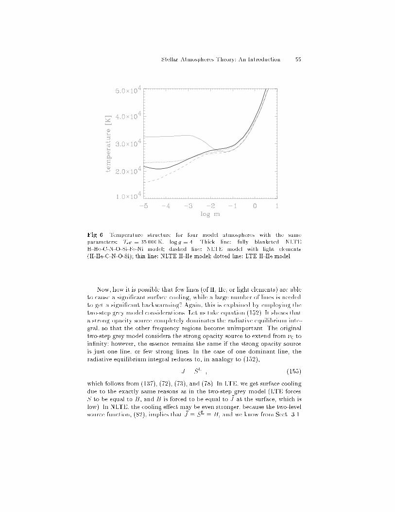
Stellar Atmospheres Theory� An Introduction ��

Fig� �� Temperature structure for four model atmospheres with the sameparameters� Te� � � ���K� log g � � Thick line� fully blanketed NLTEH�He�C�N�O�Si�Fe�Ni model� dashed line� NLTE model with light elements�H�He�C�N�O�Si�� thin line� NLTE H�He model� dotted line� LTE H�He model�

Now� how it is possible that few lines �of H� He� or light elements� are ableto cause a signicant surface cooling� while a large number of lines is neededto get a signicant backwarming� Again� this is explained by employing thetwo�step grey model considerations� Let us take equation ������ It shows thata strong opacity source completely dominates the radiative equilibrium inte�gral� so that the other frequency regions become unimportant� The originaltwo�step grey model considers the strong opacity source to extend from � toinnity however� the essence remains the same if the strong opacity sourceis just one line� or few strong lines� In the case of one dominant line� theradiative equilibrium integral reduces to� in analogy to ������

!J � SL � �����

which follows from ������ ����� ����� and ����� In LTE� we get surface coolingdue to the exactly same reasons as in the two�step grey model �LTE forcesS to be equal to B� and B is forced to be equal to !J at the surface� which islow�� In NLTE� the cooling e�ect may be even stronger� because the two�levelsource function� ����� implies that !J � SL � B� and we know from Sect� ����

�� I� Hubeny

that the two�level atom source function decreases signicantly towards thesurface�

On the other hand� the backwarming e�ect is primarily caused by blockingof the �ux by additional opacity sources the more extended �in the frequencyspace� the blocking is� the larger the backwarming �recall ����� and subse�quent discussion�� The actual strength of a line does not matter so muchas soon as it is able to e ciently block the �ux� Therefore� a single narrowand very strong line is quite e cient in the surface cooling� but relativelyine cient in the backwarming�

There is still one remaining puzzling feature� Why� in view of all whatwas said above� we obtain a large surface heating in the NLTE H�He models�This was indeed a big surprise when the e�ect was rst discovered by Auerand Mihalas ������� who have also provided its physical explanation� Thee�ect is related� but not equivalent� to another� previously discovered NLTEsurface temperature rise� called the Cayrel mechanism �Cayrel ������

The explanation of the Auer�Mihalas temperature rise goes as follows�It is true that lines always cause a surface cooling� However� in NLTE� aline radiation also in�uences the atomic level populations� From Sect� ��� weknow that the main e�ect of line transfer is to overpopulate the lower level ofa line transition� Considering Lyman and Balmer lines thus gives rise to anoverpopulation of the hydrogen n � � and n � � states� and consequently toincreasing the e ciency of the Lyman and Balmer continua� Since they areheating continua� this leads to an additional heating at the surface� Thereis a competition between this heating and traditional surface cooling causedby the Lyman and Balmer lines� but in the present case the indirect heatingwins�

However� interesting as it may be from the theoretical point of view� theindirect heating due to the hydrogen �and to a lesser extent the He II� linesis in reality usually wiped out by the e�ect of metal lines �as it is in thecase displayed in Fig� ��� Nevertheless� the Auer�Mihalas heating survives formetal�poor atmospheres� where it may give rise to observable e�ects in thehydrogen line proles �e�g� for hot DA white dwarfs � see Lanz and Hubeny���� for a discussion and original references��

Finally� I stress that the behavior of temperature at the surface shouldnot be overinterpreted� It only in�uences observed spectrum features whichcorrespond to the strongest opacity sources� like the very cores of strongestlines �e�g� the C IV resonance lines in the present case�� Yet� these featuresmay in reality be more in�uenced by a stellar wind� which is neglected inthe hydrostatic models anyway� Therefore� the most important e�ect of lineblanketing is its in�uence on temperature in the deeper layers�

Stellar Atmospheres Theory� An Introduction ��

� Using Model Atmospheres to Analyse Observed

Spectra

So far� we have been mostly concerned with the question of how the modelstellar atmospheres are constructed� In this chapter� we will discuss another�and equally important� question of how these models are used to addressgeneral astrophysical questions�

�� A Scheme of Spectroscopic Diagnostics

As was stated before� the observed spectrum is practically the only infor�mation about a star we have� The process of deducing stellar properties fromits spectrum is therefore called spectroscopic diagnostics� This is a multi�stepprocess with many interlinked steps� It is schematically displayed in Fig� ��

The basic step is input physics� By this term we mean a selection ofthe basic physical assumptions under which the medium is being described�i�e�� which processes and phenomena are neglected which equilibrium con�ditions are assumed to hold� etc��� The basic assumptions then determine theequations to be solved� They also tell us what are the basic input parametersof the model construction� For instance� when adopting the assumption of aplane�parallel atmosphere in the hydrostatic and radiative equilibrium� theinput model parameters are the e�ective temperature� surface gravity� andchemical composition� These parameters are �basic� from the point of con�structing model atmospheres� yet they are related to other parameters whichmay be viewed as more fundamental� like stellar mass� radius� and luminosity�The latter parameters are fundamental if one considers a certain instant ofthe stellar life� Yet� taking into account more extended input physics �i�e��adding the stellar evolution theory�� we may then consider even more funda�mental parameters like the initial stellar mass� initial composition� and theage�

Likewise� going to more complex models� like for instance the uniedphotosphere�wind models� we have di�erent input parameters depending onthe level of physical description we adopt� In a simple theory we have� inaddition to the stellar mass� radius� and luminosity� two additional inputparameters � the mass loss rate and the wind terminal velocity �see Lamers�this volume�� Yet� in a more involved physical picture we may come up witha relation between the wind parameters and other parameters�

Sometimes the additional input parameters make up for the lack of ad�equate physics� Typical examples are the so�called microturbulent velocitywhich is often used for describing short�scale non�thermal motions or themixing length parameter used in the mixing�length theory of convection� Anexample from a somewhat di�erent yet related eld is the ��parameter fordescribing a turbulent viscous dissipation in accretion disks� All such inputparameters are convenient parameters which allow us to construct modelseven if we do not really know what is going on� Their values are constrained

�� I� Hubeny

Fig� �� A sketch of the individual steps of astrophysical spectroscopic diagnosticsand their interconnections

Stellar Atmospheres Theory� An Introduction ��

by agreement between theoretical predictions and observations it is gener�ally believed that a more fundamental physics will either determine theirvalues from other structural parameters� or will get rid of them completely�Nevertheless� there are cases where such parameters are very useful� for in�stance when a �better physics� would require an enormously complicated andtime�consuming modeling�

The input physics� which tells us which equations are to be solved� thusin�uences profoundly the next step� numerics� By this term we understandall the work necessary to develop a code for computing model stellar atmo�spheres� This involves adopting appropriate methods provided by numericalmathematics or� often� developing new methods suited to a particular mod�eling purpose �a good example being the ALI method�� This also involvesa lot of computer programming and� the most time�consuming part� codedebugging and testing�

Having developed a stellar atmosphere code� one may proceed to the nextstep� model atmospheres� It is depicted in Fig� � as a distinct step fromnumerics� despite the fact that it could have been a part of the Numericsbox� Usually� a stellar atmosphere code contains a large number of variousnumerical options and tricks� One usually needs a lot of experience to copesuccessfully with various numerical problems �typically a slow convergenceor divergence of iterations�� and to nd proper options to coax the code towork� Sometimes the author of the code builds a grid of models him or herself�typical example being Bob Kurucz�� but it is still useful that a code itself isbeing available to the whole community� This is because the number of inter�nal input parameters may be enormous to make it reasonable to construct asu ciently dense� all�purpose grid� Many codes for stellar atmospheric mod�eling are indeed publicly available� �

The last step of the �theoretical� branch of the spectroscopic diagnosticprocedure is spectrum synthesis� which yields the main product� the syn�

thetic spectrum� It will be discussed in detail in the next section�

It should be realized that not all of the above steps have to be donein analyzing a particular object� One may work� for instance� with a pre�calculated grid of model atmospheres and construct only synthetic spectra�One may even work with an existing grid of synthetic spectra one then avoidsthe theoretical part completely�

I will not discuss the other� �observational�� branch of diagnostics� Themain steps are taking the rough data �by ground�based or space�based in�struments� � the step observations � and subsequent data reductions�The nal product is a well�calibrated observed spectrum�

Now comes the crucial part of the spectroscopic diagnostics� the com�

� The most extended collection of existing modeling codes is maintained on theCCP� �Collaborative Computer Project No� � on the Analysis of AstronomicalSpectra� library � Je�ery ������� The library is also available via WWW on theaddress http���star�arm�ac�uk�ccp��

�� I� Hubeny

parison of the observed and theoretical spectra� The actual procedure to beperformed in this step is discussed in detail in Sect� ���� Here� I will only stressthe signicance of this step in the global context� Above all� the comparisondetermines the values of basic input parameters� One may proceed iteratively�after an initial guess of input parameters and constructing the rst syntheticspectrum� the comparison step suggests new values of basic input parame�ters� which are then used for constructing a new model atmosphere and newsynthetic spectrum� and the process is repeated� Alternatively� one may rstconstruct a grid of synthetic spectra around the most probable values of basicparameters� and to determine their nal values by some sort of ���tting�

However� the most important point to realize is that the comparison stepdoes not merely serve to determine values of model input parameters� It mayhappen that we are not able to match observations for any combination ofinput parameters� Then we have to go back to the input physics step� and re�vise the basic physical assumption under which the models were constructed�This may of course lead to a revision �or even to a rewriting� of the computerprogram and consequently to reconstructing the model grid� But by this con�nection we actually learn the most important part of all � the physics�

In Fig� �� the dashed line drawn from the comparisons step to the nu�merics step is meant to indicate that lack of agreement between observationsand theory does not have to be caused by an inadequacy of adopted physicaldescription� but also by an inadequate numerical treatment of otherwise cor�rect equations� The most trivial example of this phenomenon is a hidden bugin the program� which does not in�uence the results in some cases �usuallythose used for testing�� but may have a dramatic e�ect in others� Also� thismay indicate an insu cient accuracy or inadequacy of adopted numericalmethod�s� for solving a given set of equations� for inverting matrices� etc�Another example are various numerical approximations for atomic param�eters� �e�g� polynomial expansions for transition cross�section or collisionalrates� which are derived for a certain parameter range� but are not applicablefor others� etc�� etc��

Finally� an unsuccessful match of observations and theory may revealthat the observations are at fault� For instance� an UV spectrum of a starmay by contaminated by a contribution from a close object not seen in theoptical region� Also� the data reduction step may be at fault � for instance apersistent mismatch of observations and models for various objects may leadto a discovery of an error in �ateld corrections� or an unexpected presenceof scattered light in the spectrograph� etc�

�� Spectrum Synthesis

Ideally� there should be a one�to�one correspondence between a model at�mosphere �the structure�� and the synthetic spectrum� In other words� toevery model atmosphere there should correspond a unique emergent spec�trum� However� in the real life the model structure is always computed using

Stellar Atmospheres Theory� An Introduction ��

a simplied treatment of chemical species � some of them do not in�uencethe atmospheric structure signicantly and are therefore omitted �like� forinstance� Li� etc��� or are treated in a simplied way when constructing themodel�

However� one needs to include all the opacity sources available� lines andcontinua� when producing the synthetic spectrum� One can easily a�ord that�Since the temperature� electron density� and atomic level populations arespecied by the model� the calculation of the synthetic spectrum consists ofa simple wavelength�by�wavelength formal solution of the radiative transferequation� with the absorption and emission coe cients given by ����� and������ However� the summation over line transitions may actually includehundreds or even thousands of individual spectral lines contributing at a sin�gle wavelength point� This feature� and the very fact that we have to dealwith literally millions of lines� make an e cient coding of this problem non�trivial� The most widely used general purpose codes of this kind are SYNTHE�Kurucz ������ which is designed to produce spectra for Kurucz model atmo�spheres and SYNSPEC �Hubeny� Lanz� and Je�ery ������ which calculatesspectra for NLTE models created by TLUSTY� but works for Kurucz modelsas well�

Another important point� an input model atmosphere is constructed as�suming certain abundances of chemical species� In order to be strictly con�sistent� one would have to consider the same abundances in the spectrumsynthesis as well� However� due to the same reasons as put forward above� itis permissible to use di�erent abundances in the spectrum synthesis step� It isclear that for �unimportant� species� one may change their abundance to anyreasonable value� However� one should be careful with changing abundancesof �important� species� like He� C� N� O� etc� signicantly� If this is done� it isrecommended to recalculate a full model atmosphere using these new valuesof abundances� This will not only show whether the previous approach wasreasonably accurate� but also the new model may subsequently be used for ane tuning of abundances�

It should be realized that the calculation of the nal synthetic spectrumto be compared to observations involves two steps�

�� producing the net emergent spectrum �radiation �ux at the stellar sur�face� as discussed above and

�� performing a convolution with rotational and�or instrumental broaden�ing�

Since a star generally rotates� one has to add contributions from all sur�face elements taking into account the Doppler shift due to the local projectedrotational velocity� This procedure is described in detail for instance in Gray������� If one assumes a certain a priori given limb�darkening law �i�e� thedependence of specic intensity on ��� one may perform the rotational convo�lution with the radiation �ux otherwise� the rotational convolution needs a

�� I� Hubeny

specication of radiation intensities� The procedure is easy for well�behaving�spherically�symmetric stars� However� one may face complications either be�cause of non�sphericity �for instance that implied by extremely fast rotation��or by departures from surface homogeneity �various starspots� etc��� or for acomplicated pattern of velocity elds at the stellar surface �non�radial pulsa�tions� macroturbulence� etc���

Finally� to be able to compare the predicted spectrum to observations� onehas to reproduce numerically a conversion of the incoming stellar spectrumby the spectrograph� In practice� this usually means accounting for a nitespectrum resolution of a spectrograph by convolving the net spectrum witha known instrumental broadening function �usually a Gaussian with a givenFWHM�� One can also include an instrumental spectrum sensitivity functionat this stage� The nal result of this step is a predicted spectrum which isdirectly comparable to the observed one�

�� Spectrum Fitting

The spectrum tting is the procedure of nding the model spectrum that tsthe observed spectrum best� It may be done by two di�erent ways�

i� a �consecutive model construction� procedure� which consists of a�computing rst a small number of initial models for some initial estimates ofthe basic parameters b� nding the next estimate of basic model parameters�either by an educated guess� or by using more sophisticated mathematicaltechniques � for instance the Amoeba optimized search package � Press etal� ������ and comparing the resulting spectra to observations� The processis repeated until the criteria for a successful match are satised� The basiccharacteristics of this approach is that one does not need any precalculatedgrid of models instead� the models are calculated on the way of getting closerand closer to the nal model� Obviously� this procedure is e cient only if ane�ort to generate a model spectrum from scratch is reasonably small�

ii� a �grid�tting� procedure� which consists in having a precalculated gridof spectra� and nding a model which produces the best t� One may eithernd the best�t model �i�e� one of the models of the grid�� or nd the best�tparameters by interpolating in the model grid� assuming that the syntheticspectra corresponding to model parameters in between the grid values maybe approximated by an interpolation of tabulated model spectra� If the gridhas a su ciently small step in basic stellar parameters� this procedure is quitesatisfactory�

Let us take an example of determining basic stellar parameters for OBstars from observed hydrogen and helium lines� Let us further assume thatthe mass loss rate is su ciently low so that all the observed lines originatein the stellar photosphere� i�e� their proles may be interpreted by means ofhydrostatic model atmospheres� Finally� let us assume that we are tting theobserved spectra by means of simple H�He model atmospheres� This meansthat the grid of spectra depends on ve input parameters� Te� � log g� Y �the

Stellar Atmospheres Theory� An Introduction �

helium abundance�� vtb �microturbulent velocity�� and v sin i �projected ro�tational velocity i being the inclination of the rotation axis with respect tothe direction to the observer�� One may either determine all ve of them bya ���tting� or to determine some of them independently� and to t only asubset of parameters� A typical case for OB main�sequence stars is to deter�mine vtb and v sin i from metal lines� and to determine the three remainingparameters by a line prole tting� Sometimes� even Y may be determinedindependently �from proles or equivalent widths of lines of the dominant ionof helium for which the proles are not so sensitive to Te� and logg�� Oneis then left with tting the observed hydrogen and helium line proles withonly a ��dimensional grid of spectra which depend only on Te� and logg�

There are two options to perform the actual tting�

a� tting both parameters simultaneously or

b� using the �t diagrams� This consists in keeping one parameter xed �typ�ically log g�� and nding such a value of Te� which ts the observed prolebest� One then goes to the next grid value of logg� and repeats the tting�Every tted spectral line then denes a curve in the Te��logg plane� on whichthe best�t values of Te� and log g are located� Ideally� all curves should in�tersect in one single point� which then determines the overall best t valuesof Te� and log g� In reality� one usually does not get such a good t� butat least one should obtain a relatively small region in the Te��logg planewhere the curves intersect� If one single spectral line denes a signicantlydi�erent t curve� it is a strong indication that something on the theoreticalor observational level was incorrect�

The t diagram method is illustrated on the following example� I haveconstructed a grid of NLTE H�He model atmospheres with e�ective temper�atures between ����� and ����� K� in steps of ���� K� and for logg between��� to ���� in steps of ����� All models have a solar abundance of helium�I will not t an actual observed spectrum instead� I will pretend that the�observed� spectrum is the synthetic spectrum computed for a fully metalline�blanketed NLTE model for Te� � �� ��� K� and log g � ��

This example will illustrate two features namely i� what the t diagramslook like� and ii� what error one makes if the spectrum is tted by simple H�He model atmospheres instead of by line�blanketed models� The t diagramfor H� He I and He II lines is shown in Fig� �� A very interesting resultis that the H�He models would determine the best t parameters Te� ��� ��� K� and log g � �� In other words� the H�He models will overestimatethe deduced e�ective temperature� which is not surprising in view of thediscussion presented in Sect� ���� namely that the local temperature in theH�He models in regions where H and He lines are formed is lower than in theline�blanketed models �no backwarming��

� I� Hubeny

Fig� �� A t diagram for tting the H� He I� He II line pro les by means of NLTEH�He model atmospheres� The �observed� spectrum is in fact a synthetic spectrumcomputed for a fully metal line�blanketed NLTE model for Te� � � ��� K� andlog g � � Squares� hydrogen lines �H� to H��� triangles� He I lines ��� ��� ������ �A�� stars� He II lines ��� ���� ���� ��� ��� �A��

�� Determination of Fundamental Stellar Parameters

Here we will only be concerned with the question how the fundamental stellarparameters are determined from a photospheric analysis� i�e� by analyzing theobserved stellar spectrum by means of hydrostatic model atmospheres� Animportant part of this procedure� which is nevertheless often forgotten� isto verify that the deduced stellar properties are indeed consistent with theassumption of hydrostatic equilibrium�

The fundamental stellar parameters to be determined are the stellar mass�M�� radius� R�� and luminosity� L�� In general� we do not know the distanceto the star� d� so we add this quantity to the list� even if it does not representan intrinsic stellar property� �There are� obviously� other fundamental stellarparameters� like the chemical composition� rotational velocity� etc� For thepurposes of this section� we assume that they are determined independentlyof the four fundamental parameters listed above��

The parameters which we determine directly from observations are the

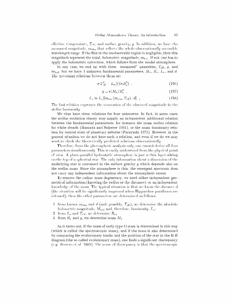
Stellar Atmospheres Theory� An Introduction ��

e�ective temperature� Te� � and surface gravity� g� In addition� we have themeasured magnitude� mobs that re�ects the whole observationally accessiblewavelength range� If the �ux in the unobservable region is negligible� then thismagnitude represent the total� bolometric� magnitude�mbol� If not� one has toapply the bolometric correction� which follows from the model atmosphere�

In any case� we end up with three �measured� quantities� Te� � g� andmbol� but we have � unknown fundamental parameters� M�� R�� L�� and d�The governing relations between them are

� T �e� � L�����R

��� � �����

g � GM��R�� � �����

L� � L� �mbol �mobs� Te�� � d� � �����

The last relation expresses the conversion of the observed magnitude to thestellar luminosity�

We thus have three relations for four unknowns� In fact� in some casesthe stellar evolution theory may supply an independent additional relationbetween the fundamental parameters� for instance the mass�radius relationfor white dwarfs �Hamada and Salpeter ������ or the mass�luminosity rela�tion for central stars of planetary nebulae �Paczynski ������ However� in thegeneral situation we do not have such a relation� and even if we do we maywant to check the theoretically predicted relations observationally�

Therefore� from the photospheric analysis only� one cannot derive all fourparameters simultaneously� This is easily understood from the physical pointof view� A plane�parallel hydrostatic atmosphere is just a thin layer sittingon the top of a spherical star� The only information about a dimension of theunderlying star is contained in the surface gravity g which depends also onthe stellar mass� Since the atmosphere is thin� the emergent spectrum doesnot carry any independent information about the atmospheric extent�

To remove the radius�mass degeneracy� we need either independent geo�metrical information �knowing the radius or the distance�� or an independentknowledge of the mass� The typical situation is that we know the distance d�the situation will be signicantly improved when Hipparchos parallaxes arereleased� then the other parameters are determined as follows�

�� from known mobs and d �and� possibly� Te��� we determine the absolutebolometric magnitude� Mbol and� therefore� luminosity� L�

�� from L� and Te� � we determine R��� from R� and g� we determine mass M�

As it turns out� if the mass of early�type O stars is determined in this way�which is called the spectroscopic mass�� and if the mass is also determinedby comparing the evolutionary tracks and the position of the star in the H�Rdiagram �the so�called evolutionary mass�� one nds a signicant discrepancy�e�g� Herrero et al� ������ The sense of discrepancy is that the spectroscopic

�� I� Hubeny

masses are systematically lower than the evolutionary masses� The discrep�ancy arises either by inaccuracies of the stellar atmospheres theory� or thestellar evolution theory� or� most likely both� From the stellar atmospheresside� there has been a recent progress in understanding the reasons for thediscrepancy �e�g� Lanz et al� ������ However� the problem is not yet solved�and presents a challenge for future research�

Acknowledgements

It is a pleasure to thank the organizers of the �th European AstrophysicsDoctoral Network Summer School for the invitation to give these lectures� Iwould also like to thank my colleagues in the audience and my co�lecturers forstimulating discussions� I would like to thank Thierry Lanz� Alex de Koter�Steve Shore� and Tom Brown for their careful reading of the manuscript ando�ering a number of useful suggestions�

References

Allard� F� Hauschildt� P�H� ������� ApJ ���� Anderson� L� S� ������� ApJ ��� ��Anderson� L� S� ������� in Numerical Radiative Transfer� ed� by W� Kalkofen� Cam�bridge Univ� Press� Cambridge� p� ��

Anderson� L� S� ������� ApJ ��� ���Anderson� L� S� ������� in Stellar Atmospheres� Beyond Classical Models� ed� byL� Crivellari� I� Hubeny� and D�G�Hummer� NATO ASI Series C � � Kluwer�Dordrecht� p� ��

Anderson� L� S�� Grigsby� J�A� ������� in Stellar Atmospheres� Beyond Classical

Models� ed� by L� Crivellari� I� Hubeny� and D�G�Hummer� NATO ASI Series C� � Kluwer� Dordrecht� p� ��

Auer� L�H� ������� in Numerical Radiative Transfer� ed� by W� Kalkofen� CambridgeUniv� Press� Cambridge� p� ���

Auer� L�H� ������� in Stellar Atmospheres� Beyond Classical Models� ed� by L� Criv�ellari� I� Hubeny� and D�G�Hummer� NATOASI Series C � � Kluwer� Dordrecht�p� �

Auer L�H�� Mihalas D� ������� ApJ ���� ��Auer� L�H�� Mihalas� D� ������� MNRAS ��� ��Avrett� E�H�� Hummer� D�G� ������� MNRAS ��� ���B�ohm�Vitense� E� ������� Introduction to Stellar Astrophysics II� Stellar Atmo�

spheres� Cambridge Univ� Press� CambridgeButler� K�� Giddings� J� ������� in Newsletter on Analysis of Astronomical Spectra

No� �� Daresbury Laboratory� Daresbury� EnglandCannon� C�J� ������ J� Quant� Spectrosc� Radiat� Transfer ��� ���Carlsson� M� ������� A Computer program for Solving Multi�Level Non�LTe Radia�

tive Transfer Problems in Moving or Static Atmospheres� Report No� � UppsalaAstron� Obs�

Castor� J� I�� Abbott� D� C�� Klein� R� I� ������� ApJ� ��� ���

Stellar Atmospheres Theory� An Introduction ��

Castor� J�I�� Dykema� P�G�� Klein R�I� ������� in Stellar Atmospheres� Beyond Clas�

sical Models� ed� by L� Crivellari� I� Hubeny� and D�G�Hummer� NATOASI SeriesC � � Kluwer� Dordrecht� p� ��

Castor� J�I�� Dykema� P�G�� Klein� R�I� ������� ApJ� ���� ���

Cayrel� R� ������ C� R� Acad� Sci� Paris ���� ��

Chandrasekhar� S� ������� Radiative Transfer� Dover� New York

Crivellari� L�� Hubeny� I�� Hummer D� G� �Eds�� ������� Stellar Atmospheres� Be�yond Classical Models� NATO ASI Series C ��� �Dordrecht� Kluwer�

de Koter� A�� Schmutz� W�� Lamers� H� J� G� L� M� ������ A�A � ���� ���

Dreizler� S�� Werner� K� ������ A�A� ���� ����

Feautrier� P� ������ C� R� Acad� Sci� Paris ���� ���

Gabler� R�� Gabler� A�� Kudritzki� R� P�� Puls� J�� Pauldrach� A� ������� A�A� �������

Garmany� C�D� �Ed�� ������� Properties of Hot Luminous Stars� PASP Conf� Ser�Vol� �� Astron� Soc� Paci c� San Francisco

Gray� D�F� ������� Observations and Analysis of Stellar Photospheres� �nd ed��Cambridge Univ� Press� Cambridge

Griem� H�R� ������ Spectral Line Broadening by Plasmas� Acad� Press� New York

Gustafsson� R�� Bell� R�A�� Eriksson� K�� Nordlund� A� ������� A�A ��� ��

Hamada� T�� Salpeter� E�E� ������� ApJ ���� ��

Hamann� W��R� ������� A�A ���� �

Heber� U�� Je�ery� C�J� �Eds�� ������� The Atmospheres of Early�Type Stars� LectureNotes in Phys� ��� Springer� Berlin� p� ��

Herrero� A�� Kudritzki� R�P�� Vilchez� J�M�� Kunze� D�� Butler� K�� Haser� S� �������A�A ���� ���

Hillier� D�J� ������� A�A � ���� ���

Hubeny� I� ������� in Progress in Stellar Spectral Line Formation Theory� ed� byJ�E� Beckman and L� Crivellari� NATO ASI Series C ���� Reidel� Dordrecht

Hubeny� I� ������� A�A ���� �

Hubeny� I� ������� Comp� Phys� Comm� ��� ��

Hubeny� I� ������� in The Atmospheres of Early�Type Stars� ed� by U� Heber andC�J� Je�ery� Lecture Notes in Phys� ��� Springer� Berlin� p� ��

Hubeny� I�� Lanz� T� ������� A�A ���� ���

Hubeny� I�� Lanz� T� ������� ApJ ��� ���

Hubeny� I�� Lanz� T�� Je�ery� C� S� ������ in Newsletter on Analysis of AstronomicalSpectra No� ��� Ed� Je�ery C� S�� St Andrews Univ�� St Andrews� �

Hummer� D�G� ������� J� Quant� Spectrosc� Radiat� Transfer ��� ���

Ivanov� V�V� ������ Transfer of Radiation in Spectral Lines� English languagetranslation of Radiative Transfer and the Spectra of Celestial Bodies� transl�by D�G� Hummer� NBS Special Publ� No� ��� National Bureau of Standards�Washington

Je�eries� J� ������� Spectral Line Formation� Blaisdel� Waltham

Je�ery� C� S� ������� in Newsletter on Analysis of Astronomical Spectra No� ��� Ed�Je�ery C� S�� CCP�� �St Andrews� St Andrews Univ���

Je�ery� C�J�� Heber� U� �Eds�� ������� Hydrogen�De�cient Stars� PASP Conf� Ser�Vol� ��� Astron� Soc� Paci c� San Francisco

Johnson� H�R�� Bernat� A�P�� Krupp� B�� Bell� R�A� ������� ApJ ���� ���

�� I� Hubeny

Kalkofen� W� �Ed�� ������ Methods in Radiative Transfer� Cambridge Univ� Press�Cambridge

Kalkofen� W� �Ed�� ������� Numerical Radiative Transfer� Cambridge Univ� Press�Cambridge

Kudritzki� R�P� ������� The Atmospheres of Hot Stars� Modern Theory and Obser�

vation� in Radiation in Moving Gaseous Media� ed� by� Y� Chmielewski and T�Lanz� ��th Advanced Course� Swiss Soc� of Astron� and Astrophys�� Geneva

Kudritzki� R� P�� Hummer D� G� ������� ARA�A ��� �Kurucz� R� L� ������� Smithsonian Astrophys� Obs� Spec� Rep� No� ��Kurucz� R� L� ������� ApJS �� �Kurucz� R� L� ������ Kurucz CD�ROM No� �� Smithsonian Astrophys� Obs�Lanz� T� � Hubeny� I� ������� ApJ ��� ���Lanz� T�� de Koter� A�� Hubeny� I�� Heap� S� R� ������� ApJ ���� ��Mihalas� D� ������� Stellar Atmospheres� Freeman� San FranciscoMihalas D�� Heasley J�N�� Auer L�H� ������� A Non�LTE model stellar atmospheres

computer program� NCAR�TN�STR���� NCAR� BoulderPauldrach� A�W�A� Puls� J�� Kudritzki� R�P� ������� A�A� ���� ��Paczynski� B�E� ������� Acta Astr� ��� ��Olson� G�L�� Auer� L�H�� Buchler� J�R� ������� J� Quant� Spectrosc� Radiat� Trans�fer ��� � �OAB�

Olson� G�L�� Kunasz� P�B� ������� J� Quant� Spectrosc� Radiat� Transfer ��� ��Oxenius� J� ������� Kinetic Theory of Particles and Photons� Springer�Verlag�Berlin Heidelberg

Press� W�H�� Flannery� B�P�� Teukolsky� S�A�� Vetterling� W�T� ������� NumericalRecipes� Cambridge Univ� Press� Cambridge

Rutten� R�J� ������� Radiative Transfer in Stellar Atmospheres� �nd WWW edition�June ��� ����� Robert J� Rutten� Utrecht� Netherlands

Rybicki� G�B� ������� J� Quant� Spectrosc� Radiat� Transfer ��� ���Rybicki� G�B� ������ in Methods in Radiative Transfer� ed� by W� Kalkofen� Cam�bridge Univ� Press� Cambridge� p� ��

Rybicki� G�B� and Hummer� D�G� ������� A�A� ���� ���Rybicki� G�B� and Hummer� D�G� ������� A�A� ���� ����Rybicki� G�B�� Lightman� A�P� ������� Radiative Processes in Astrophysics� Wiley�Interscience� New York

Scharmer� G�B� ������� ApJ ��� ���Schaerer� D�� Schmutz� W� ������ A�A ���� ��Sellmaier� F�� Puls� J�� Kudritzki� R�P�� Gabler� A�� Gabler� R�� Voels� S�A� ������A�A� ���� �

Shu� F�H� ������� The Physics of Astrophysics I� Radiation� University ScienceBooks� Mill Valley

Sten�o� J�O� ������ Solar Magnetic Fields� Polarized Radiation Diagnostics�Kluwer� Dordrecht

Tsuji� T� ������� Pub� Astron� Soc� Japan ��� �Werner� K� ������� A�A ���� ���Werner� K� ������� in Numerical Radiative Transfer� ed� by W� Kalkofen� CambridgeUniv� Press� Cambridge� p� ��

Werner� K� ������� A�A ���� ���Werner� K�� Husfeld� D� ������� A�A ���� ��