A Brief Introduction to Neural Networks

Richard D. De Veaux Lyle H. Ungar

Williams College University of Pennsylvania

Abstract

Arti�cial neural networks are being used with increasing frequency for high dimen-

sional problems of regression or classi�cation. This article provides a tutorial overview

of neural networks, focusing on back propagation networks as a method for approx-

imating nonlinear multivariable functions. We explain, from a statistician's vantage

point, why neural networks might be attractive and how they compare to other modern

regression techniques.

KEYWORDS: neural networks; function approximation; backpropagation.

1 Introduction

Networks that mimic the way the brain works; computer programs that actually learn pat-terns; forecasting without having to know statistics. These are just some of the many claimsand attractions of arti�cial neural networks. Neural networks (we will henceforth drop theterm arti�cial, unless we need to distinguish them from biological neural networks) seem tobe everywhere these days, and at least in their advertising, are able to do everything thatstatistics can do without all the fuss and bother of having to do anything except buy a pieceof software.

Neural networks have been successfully used for many di�erent applications; Pointers tosome of the vast literature are given at the end of this article. In this article we will attemptto explain how one particular type of neural network, feedforward networks with sigmoidalactivation functions (\backpropagation networks") actually works, how it is \trained", andhow it compares with some more well known statistical techniques.

As an example of why someone would want to use a neural network, consider the problemof recognizing hand written ZIP codes on letters. This is a classi�cation problem, where theinputs (predictor variables) might be a vector of grey scale pixels measuring the darknessof each small subdivision of the character. The desired response, y, is the digit of the ZIP

1

code. The modeling problem could be thought of as �nding an appropriate relationshipy = f(x; �), where � is a set of unknown parameters. This is a large problem: x may beof length 1,000 or more. The form of f is unknown | certainly not linear | and mayrequire tens of thousands of parameters to �t accurately. Large data sets with hundreds ofthousands of di�erent handwritten ZIP codes are available for estimating the parameters.Neural networks o�er a means of e�ciently modeling such large and complex problems.

Neural networks di�er in philosophy from many statistical methods in several ways. First,a network usually has many more parameters than a typical statistical model. Becausethey are so numerous, and because so many combinations of parameters result in similarpredictions, the parameters become uninterpretable and the network serves as a black boxestimator. Therefore, the network, in general, does not aid in understanding the underlyingprocess generating the data. However, this is acceptable, and even desirable in many otherapplications. The post o�ce wants to automatically read ZIP codes, but does not care whatthe form of the functional relationship is between the pixels and the numbers they represent.This is fortunate, since there is little hope of �nding a functional relationship which will coverall of the variations in handwriting which are encountered. Some of the many applicationswhere hundreds of variables may be input into models with thousands of parameters includemodeling of chemical plants, robots and �nancial markets, and pattern recognition problemssuch as speech, vision and handwritten character recognition.

Neural network methods share a loose inspiration from biology in that they are repre-sented as networks of simple neuron-like processors. A typical \neuron" takes in a set ofinputs, sums them together, takes some function of them, and passes the output through aweighted connection to another neuron. Neural networks are often represented as shown inFigure 1. At �rst glance, such �gures are not very revealing to a statistician. But as we willshow, many familiar statistical techniques can be represented in this framework.

Each neuron may be viewed simply as a predictor variable, or as a combination of pre-dictor variables. The connection weights are the unknown parameters which are set by a\training method". That is, they are estimated. The architecture, i.e., the choice of inputand output variables, the number of nodes and hidden layers, and their connectivity, areusually taken as given. More will be said about this later.

Actual biological neural networks are incomparably more complex than their arti�cialcounterparts. Real neurons are living cells with complex biochemistry. They transmit andprocess information by the build-up and release of ions and other chemicals, and so havememory on many di�erent time scales. Thus, their outputs are often sequences of voltagespikes, which may increase or decrease in frequency depending on what signals the neuronreceived earlier. Real neural networks also have a complex connectivity, and a variety ofmechanisms by which the networks elements and their connections may be altered.

Arti�cial neural networks retain only a small amount of this complexity and use simplerneurons and connections, but keep the idea of local computation. Many di�erent networkarchitectures are used, typically with hundreds or thousands of adjustable parameters. The

2

resulting equation forms are general enough to solve a large class of nonlinear classi�cationand estimation problems and complex enough to hide a multitude of sins.

One advantage of the network representation is that it can be implemented in massivelyparallel computers with each neuron simultaneously doing its calculations. Several commer-cial neural network chips and boards are available, but most people still use neural network\simulators" on standard serial machines. This paper will not discuss parallel hardwareimplementation, but it is important to remember that parallel processing was one of themotivations behind the development of arti�cial neural networks.

We will focus primarily on neural networks for multivariable nonlinear function approx-imation (regression) and somewhat less on the related problem of classi�cation. The mostwidely used network for these problems is the multilayer feedforward network. This is of-ten called the \backpropagation network", although backpropagation actually refers to thetraining (or estimation) method. For a more advanced introduction to other types of neu-ral networks which serve as classi�ers or as data clustering methods, see Lippman (1987)or Ripley (1994). We formally de�ne the backpropagation network in section 2. Here wealso introduce several examples that will serve us throughout the paper and discuss howto estimate the parameters in a neural network. Section 3 involves the tradeo�s betweentraining and over�tting. A brief overview of neural networks other than the backpropagationnetwork is contained in section 4. A comparison to familiar statistical methods in containedin section 5. We conclude with a brief discussion in section 6.

2 Feedforward networks with sigmoidal activation func-

tions

Consider the problem of predicting a response yl from a set of predictor variables, x1; : : : ; xLThe backpropagation network with one hidden layer is nothing more than a statistical modelof the following form:

yl = �(2)

0@

KXk=1

w2kl �(1)

0@

JXj=1

w1jkxj + �j

1A+ �k

1A (1)

where the functions �(1) and �(2) are generic transformations, known as activation functions,which may be linear or non-linear. Usually, �(1) is a sigmoidal function such as the logistic�(1)(z) = 1=(1+e�z) or �(1)(z) = tan�1(z). For regression problems, �(2) is often the identify,while for classi�cation problems it is sigmoidal as well. Sigmoidal activation functions arealso known as a squashing functions for obvious reasons. The terms �j and �k are constantsthat act as intercept terms in the model, called bias nodes.

For each k, the inner summation over j produces a weighted linear combination of thepredictors. There are K such linear combinations, referred to as \hidden layer" variables, so

3

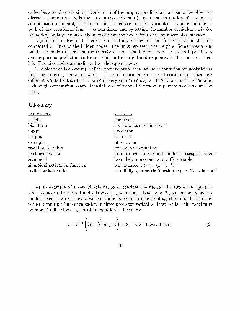
called because they are simply constructs of the original predictors that cannot be observeddirectly. The output, yl is then just a (possibly non-) linear transformation of a weightedcombination of possibly non-linear transformations of these variables. By allowing one orboth of the transformations to be non-linear and by letting the number of hidden variables(or nodes) be large enough, the network has the exibility to �t any reasonable function.

Again consider Figure 1. Here the predictor variables (or nodes) are shown on the left,connected by links to the hidden nodes. The links represent the weights. Sometimes a � isput in the node to represent the transformation. The hidden nodes act as both predictorsand responses: predictors to the node(s) on their right and responses to the nodes on theirleft. The bias nodes are indicated by the square nodes.

The bias node is an example of the nomenclature that can cause confusion for statisticians�rst encountering neural networks. Users of neural networks and statisticians often usedi�erent words to describe the same or very similar concepts. The following table containsa short glossary giving rough \translations" of some of the most important words we will beusing.

Glossary

neural nets statisticsweight coe�cientbias term constant term or interceptinput predictoroutput responseexemplar observationtraining, learning parameter estimationbackpropagation an optimization method similar to steepest descentsigmoidal bounded, monotonic and di�erentiablesigmoidal activation function for example, �(x) = (1 + e�x)�1

radial basis function a radially symmetric function, e.g. a Gaussian pdf

As an example of a very simple network, consider the network illustrated in �gure 2,which contains three input nodes labeled x1; x2 and x3, a bias node, �1, one output y and nohidden layer. If we let the activation functions be linear (the identity) throughout, then thisis just a multiple linear regression in three predictor variables. If we replace the weights wby more familiar looking notation, equation 1 becomes:

y = �(1)

0@�1 +

3Xj=1

w1j1xj

1A = b0 + b1x1 + b2x2 + b3x3: (2)

4

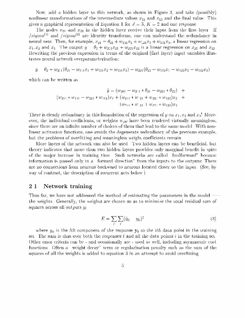
Now, add a hidden layer to this network, as shown in Figure 3, and take (possibly)nonlinear transformations of the intermediate values x11 and x12 and the �nal value. Thisgives a graphical representation of Equation 1 for J = 3, K = 2 and one response.

The nodes x21 and x22 in the hidden layer receive their input from the �rst layer. If=sigma(1) and =sigma(2) are identity transforms, one can understand the redundancy inneural nets. Then, for example, x21 = �21 +w111x1 +w121x2 +w131x3, a linear regression onx1; x2 and x3. The output y = �2 + w211x21 + w221x22 is a linear regression on x21 and x22.Rewriting the previous expression in terms of the original (�rst layer) input variables illus-trates neural network overparameterization:

y = �2 + w211(�21 + w111x1 + w121x2 + w131x3) + w221(�22 + w112x1 + w122x2 + w132x3)

which can be written as

y = (w201 + w211 � �21 + w221 � �22) +

(w211 � w111 + w221 � w112)x1 + (w211 � w121 + w221 � w122)x2 +

(w211 � w131 + w221 � w132)x3

There is clearly redundancy in this formulation of the regression of y on x1; x2 and x3! More-over, the individual coe�cients, or weights wjkl have been rendered virtually meaningless,since there are an in�nite number of choices of them that lead to the same model. With non-linear activation functions, one avoids the degenerate redundancy of the previous example,but the problems of over�tting and meaningless weight coe�cients remain.

More layers of the network can also be used. Two hidden layers can be bene�cial, buttheory indicates that more than two hidden layers provides only marginal bene�t in spiteof the major increase in training time. Such networks are called \feedforward" becauseinformation is passed only in a \forward direction" from the inputs to the outputs; Thereare no connections from neurons backward to neurons located closer to the input. (See, byway of contrast, the description of recurrent nets below.)

2.1 Network training

Thus far, we have not addressed the method of estimating the parameters in the model |the weights. Generally, the weights are chosen so as to minimize the total residual sum ofsquares across all outputs yl

E =Xl

Xi

(yli � yli)2 (3)

where yli is the lth component of the response yi to the ith data point in the trainingset. The sum is thus over both the responses l and all the data points i in the training set.Other error criteria can be - and occasionally are - used as well, including asymmetric costfunctions. Often a \weight decay" term or regularization penalty such as the sum of thesquares of all the weights is added to equation 3 in an attempt to avoid over�tting.

5

Once the network structure and the objective function have been chosen, this is simply anonlinear least squares problem, and can be solved using any of the standard nonlinear leastsquares methods. For example, the weights can be estimated by any number of optimizationmethods such as steepest descent. For relatively small problems on serial machines, conjugategradient methods work well. On parallel machines, or when one is not concerned withe�ciency, a simple gradient descent method is often used.

The famous \backpropagation" algorithm or \delta learning rule" is simply (stochastic)gradient descent. At each iteration, each weight wi is adjusted proportionally to its e�ecton the error

�wi = �dE

dwi

: (4)

The constant, �, controls the size of the gradient descent step taken and is usually takento be around 0.1 to 0.5. If � is too small, learning is slow. If it is too large, instabilityresults and the wi do not converge. The derivative dE=dwi can be calculated purely locally,so that each neuron needs information only from neurons directly connected to it. Thebasic derivation follows the chain rule: the error in the output of a node may be ascribedin part to errors in the immediately connected weights and in part to errors in the outputsof \upstream" nodes (Rumelhart, Hinton and Williams 1986). Both \batch" and \online"variations of the method are used in which, respectively, the weights are updated basedon dE=dwi for the entire data set (as above) or the weights are updated after each singleadditional data point is seen. The online method is particular useful for real time applicationssuch as vehicle control based on video camera data.

When the chain rule is implemented on a massively parallel machine, it gives rise tothe \backpropagation" in backpropagation networks: the error at an output neuron canbe partly ascribed to the weights of the immediate inputs to the neuron, and partially toerrors in the outputs of the hidden layers. Errors in the output of each hidden layer are dueto errors in the weights on its inputs. The error is thus propagated back from the outputthrough the network to the di�erent weights, always by repeated use of the chain rule.

One can achieve faster convergence by adding a \momentum term" proportional to theprevious change, �wt�1

i :

�wi = �dE

dwi

+ ��wt�1i : (5)

The momentum term approximates the conjugate gradient direction. There is an enor-mous literature on more e�cient methods of selecting weights, most of which describes waysof adjusting � and �. On standard serial computers, it is generally more e�cient to use con-jugate gradient methods, which use second derivatives (the Hessian) and line search, ratherthan gradient descent to determine � and �.

Selecting weights is, of course, a highly nonlinear problem since the function being mini-mized, E, has many local minima. When di�erent initial values for the weights are selected,di�erent models will be derived. Small random values are traditionally used to initialize

6

the network weights. Alternatively, networks can be initialized to give predictions prior totraining that replicate an approximate model of the data obtained, for example, by linearregression. Although the models resulting from di�erent initial weights have very di�erentparameter values, the �t and prediction errors generally do not vary too dramatically.

It is important to repeat that these networks are typically not used for interpretation.Since all neurons in a given layer are structurally identical, there is a high degree of collinear-ity between the outputs of the di�erent neurons, so individual coe�cients become meaning-less. Also, the network structure permits high order interactions, so there are typically nosimple substructures in the model to look at | in contrast with, for example, additive mod-els. (However, neural network users often plot the pattern of outputs of the hidden neuronsfor di�erent inputs for use as \feature detectors".) As mentioned above, this is not nec-essarily a problem, since one typically uses the network for prediction or classi�cation andnot for interpretation. For large, complex modeling problems like character recognition orspeech-to-text translation, there need not be a simple, intelligible model which is accurate.

Neural networks have a number of attractive properties which, given the usual lists oftechnical preconditions, can be rigorously proven. Given enough neurons, and hence enoughadjustable parameters, any well-behaved function can be approximated. Less obviously,neural networks can be viewed as providing a set of adaptive basis functions which put morebasis functions where the data are known to vary more rapidly. This allows much moree�cient representation for high dimensional inputs (many predictors) than using �xed basisfunctions such as polynomial regression or Fourier approximations (Barron 1996).

2.2 Example

To better understand how neural nets work on real problems, we begin with a multiplelinear regression example using a set of data from a polymer process with 10 predictorvariables x1; : : : ; x10 and a response, y. (Psichogios et al. 1993; Data are available via ftp atftp.cis.upenn.edu: pub/ungar/chemdata ).

It turns out that x5 is a linear combination of the other predictors, so for now, we restrictourselves to a regression of y on x1; :::; x4; x6; :::; x10. Linear regression gives the values shownin Table 1.

7

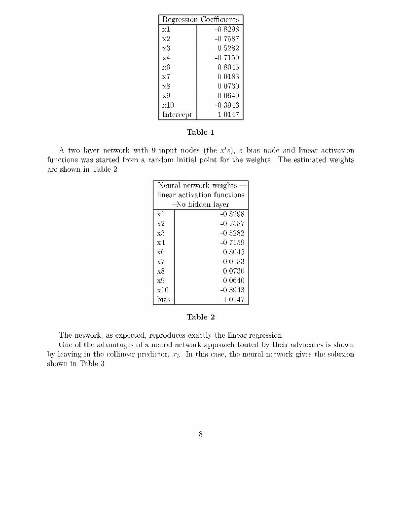
Regression Coe�cientsx1 -0.8298x2 -0.7587x3 -0.5282x4 -0.7159x6 0.8045x7 0.0183x8 0.0730x9 0.0640x10 -0.3943Intercept 1.0147

Table 1

A two layer network with 9 input nodes (the x0s), a bias node and linear activationfunctions was started from a random initial point for the weights. The estimated weightsare shown in Table 2.

Neural network weights {linear activation functions

{No hidden layerx1 -0.8298x2 -0.7587x3 -0.5282x4 -0.7159x6 0.8045x7 0.0183x8 0.0730x9 0.0640x10 -0.3943bias 1.0147

Table 2

The network, as expected, reproduces exactly the linear regression.One of the advantages of a neural network approach touted by their advocates is shown

by leaving in the collinear predictor, x5. In this case, the neural network gives the solutionshown in Table 3.

8

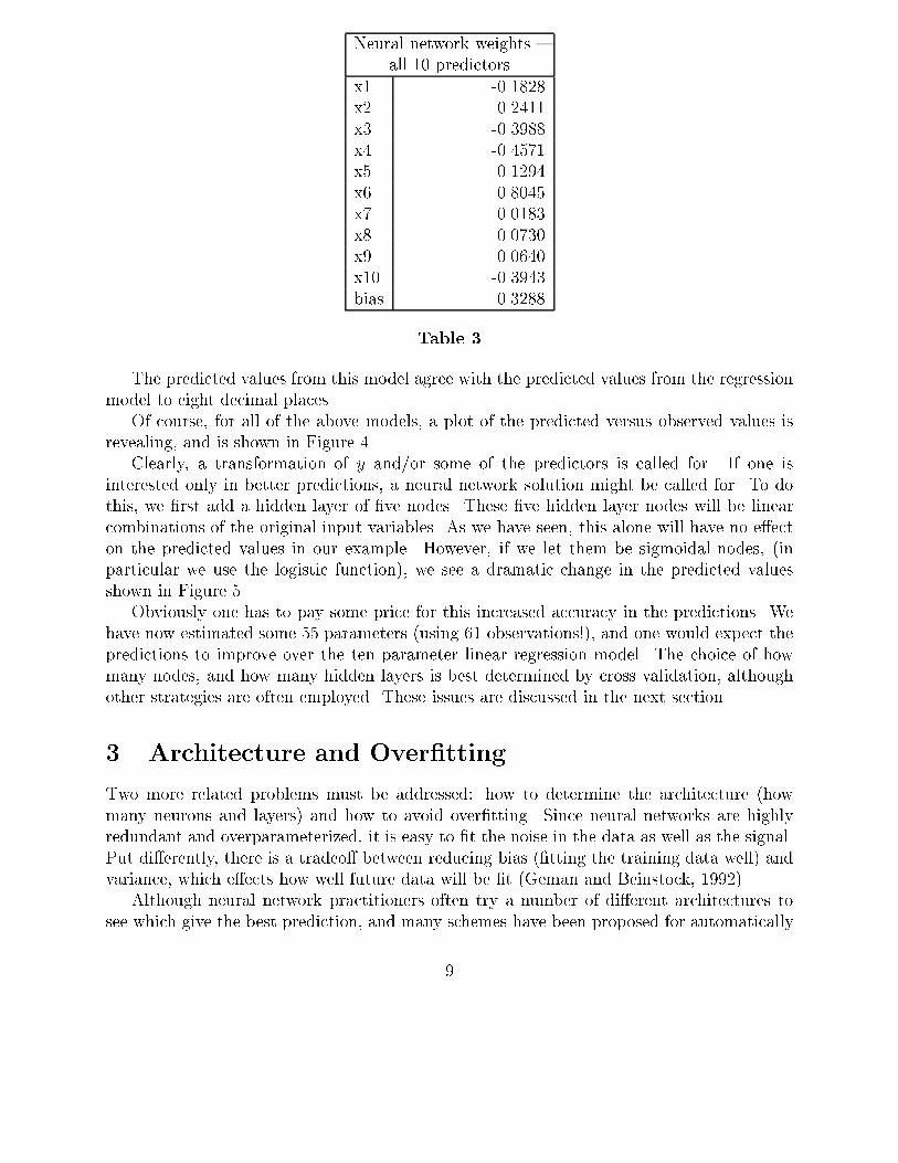
Neural network weights {all 10 predictors

x1 -0.1828x2 -0.2411x3 -0.3988x4 -0.4571x5 0.1294x6 0.8045x7 0.0183x8 0.0730x9 0.0640x10 -0.3943bias 0.3288

Table 3

The predicted values from this model agree with the predicted values from the regressionmodel to eight decimal places.

Of course, for all of the above models, a plot of the predicted versus observed values isrevealing, and is shown in Figure 4.

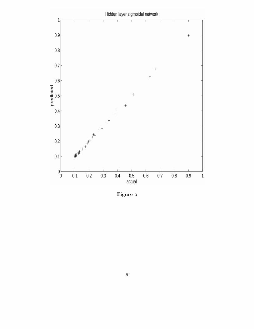
Clearly, a transformation of y and/or some of the predictors is called for. If one isinterested only in better predictions, a neural network solution might be called for. To dothis, we �rst add a hidden layer of �ve nodes. These �ve hidden layer nodes will be linearcombinations of the original input variables. As we have seen, this alone will have no e�ecton the predicted values in our example. However, if we let them be sigmoidal nodes, (inparticular we use the logistic function), we see a dramatic change in the predicted valuesshown in Figure 5.

Obviously one has to pay some price for this increased accuracy in the predictions. Wehave now estimated some 55 parameters (using 61 observations!), and one would expect thepredictions to improve over the ten parameter linear regression model. The choice of howmany nodes, and how many hidden layers is best determined by cross validation, althoughother strategies are often employed. These issues are discussed in the next section.

3 Architecture and Over�tting

Two more related problems must be addressed: how to determine the architecture (howmany neurons and layers) and how to avoid over�tting. Since neural networks are highlyredundant and overparameterized, it is easy to �t the noise in the data as well as the signal.Put di�erently, there is a tradeo� between reducing bias (�tting the training data well) andvariance, which e�ects how well future data will be �t (Geman and Beinstock, 1992).

Although neural network practitioners often try a number of di�erent architectures tosee which give the best prediction, and many schemes have been proposed for automatically

9

selecting network structure (e.g. by removing less important neurons or links), the mostcommon procedure is to select a network structure which has more than enough parametersand then to avoid the worst aspects of over�tting by the network training procedure. Thisis the strategy that was employed in the example above.

In most problems that a neural network practitioner would attack, data are abundant.In such cases, one could set aside some proportion (say half) of the data to use only forprediction after the model has been trained (parameters estimated). We call this the test set.The half used for estimation is called the training set. If one then plots mean squared erroras a function of number of iterations in the solution procedure, the error on the training datadecreases monotonically, while the error on the test set decreases initially and then passesthrough a shallow minimum and slowly increases. (See Figure 6.) The values of the weightsfrom the minimum prediction error are then used for the �nal model. For small data sets,where splitting the data into two groups will leave too few observations for either estimationor validation, in principal at least, resampling or leave-one-out training may be used eitherto determine when to stop training or to determine the optimal network size.

One would expect that for a given data set there would be an optimal number of hiddenneurons, with the optimum lying between one neuron (high bias, low variance) and a verylarge number of neurons (low bias, high variance). This is true for some data sets, but,counterintuitively, for most large data sets, increasing the number of hidden nodes continuesto improve prediction accuracy, as long as cross validation is used to stop training. To ourknowledge, although there has been extensive speculation, the reason for this has not beenexplained.

Since estimating the weights in a neural network is a nonlinear least squares problem,all of the standard nonlinear least squares solution and analysis methods can be applied.In particular, in recent years, a number of regularization methods have been proposed tocontrol the smoothness, and hence the degree of over�tting, in neural networks. As just oneexample, one can use Bayesian techniques to select network structures and to penalize largeweights or reduce over�tting (Buntine and Weigend 1991, MacKay 1992).

3.1 Example

Continuing with our regression example, we will use the hidden layer sigmoidal network with5 nodes in the hidden layer, as before. Although it is possible to choose the architecture bycross-validation, we will illustrate the procedure of using what we presume to be an adequatearchitecture (with 55 parameters for 61 observations) and to select the amount of trainingby cross-validation instead.

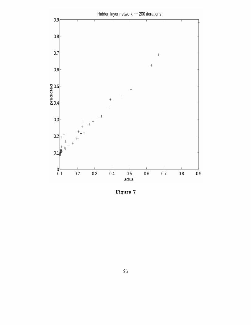
To do this, we randomly select some percentage of the data (typically 10%) to use asthe test data and use the remaining data as the training data. We then train the network,monitoring the residual sum of squares. We repeat this procedure with di�erent test dataseveral times. Looking at Figure 6, we see that the test set error decreases initially, butreaches a minimum at about 200 iterations. The training set error continues to decrease asone might expect.

10

Retraining the network on the entire data set using 200 iterations, gives a residual sumof squares of 0.0304 with the plot of predicted vs. actual values shown in Figure 7.

3.2 Second Example

If the data have a particularly simple structure a exible method like a neural network modelshould be able to reproduce it. To illustrate this, we generated 100 observations from thefollowing model:

y = 10 + 2x1 � 3x2 + x3 + �

where � � N(0; 1) A linear regression program gave:

b =

10.3726

1.2671 R^2 = 49.53

-2.9396

0.7958

Residual sum of squares = 99.30

With enough nodes and sigmoidal transfer functions, we could get a perfect �t to these data.

A network with 20 nodes in the hidden layer, allowed to train to convergence, produced a residual

sum of squares of 25.07.

>> weights20 = make_bpn(X,y,nodes,tf,[],2000);

GRADIENTS FUNCTIONS OBJECTIVE METHOD

0 1 9083

1 5 268.7 steepest descent

2 8 250.6 FR conj grad

...

2650 7953 25.07 FR conj grad

2651 7956 25.07 FR conj grad

Training terminated: no more progress

Suspecting that we may have over�t to the data here, we cross-validate by resampling 90% of

the data as training data and 10% of the data as test data. We observe the average error sum of

squares on the test data as we allow the network to train:

This suggests using 20 iterations (as opposed to 7956!!!). Restarting the training but this time

stopping the training at 20 iterations, we �nd:

>> weightscv20 = make_bpn(X,y,nodes,tf,[],20);

GRADIENTS FUNCTIONS OBJECTIVE METHOD

0 1 8811

1 4 279 steepest descent

2 7 257.8 FR conj grad

11

...

6 20 98.78 FR conj grad

Maximum number of function calls exceeded

Notice that the residual sum of squares is nearly identical to the linear regression �t.Moreover, a plot of the predicted values would indicate that predicted values from thisnetwork are nearly identical to linear regression!!

In conclusion, this cross-validation method starts with a large network, one large enoughso that if allowed to train until convergence would most likely result in �tting the train-ing data nearly perfectly. To avoid this, we stop the training early, a�ecting some sort ofregularization to a random starting point. To decide how early to stop training this largenetwork, we use the randomly chosen test sets multiple times and see where the performanceon the test set is optimized. This ad hoc method seems to produce a reasonable trade o�between �tting and over�tting and is the most commonly used method in practice. As men-tioned above, many statisticians �nd early stopping too ad hoc and prefer a more systematicregularization such replacing the error criterion Equation 3 with

E =Xl

Xi

(yli � yli)2 + �

Xj

w2j (6)

where j ranges over all the weights and � is chosen using cross validation.

4 Variations on the network theme

One of the reasons that researchers are excited about neural networks is that the networkstructure suggests new equation forms. Although networks of the form described aboveaccount for most of the commercially used networks, there is an extremely large researche�ort on alternate equational forms. This section gives a glimpse of some of the diversity inequational forms that are being studied.

Neural networks can come in many forms|so many that it appears that anything canbe turned into a neural net (see e.g, Barron et al. 1992). This is partly true, in thatany equation can be written as a set of nodes which perform operations like addition andmultiplication, and a set of links which are associated with adjustable parameters. However,there is a common spirit between the many avors of neural networks. Neural networks areinspired by biology and as such, most have neurons which either have a logistic \transferfunction," representing the saturation which occurs in real neurons, or a Gaussian transferfunction, representing \local receptive �elds." (See below.) Equally importantly, but lessoften followed, neural networks tend to have purely local training methods, i.e. one need notcompute a Jacobian or Hessian for the whole system of equations, but parameter updatingcan be done using only information which is available locally at each neuron.

One important non-biological variation on neural nets is to incorporate prior knowledgeabout a problem into the network. Neural networks can be built which have only partial

12

connectivity, when one believes that not all input variables interact. Networks can alsoincorporate �rst principles equations such as mass and energy balances (Psichogios andUngar 1992), or known linear approximations to the process being modeled. They can takedata which have been processed with a smoothing �lter or can work with the loading vectorsproduced by linear projection methods such as Principle Components Analysis (PCA) orPartial Least Squares (PLS) (Holcomb and Morari 1992, Qin and McAvoy 1992).

In another set of variations, arti�cial neural network can be made which are continu-ous in time. Besides more accurately re ecting biological neurons (an unclear advantage),continuous time networks are more naturally implemented in some types of computer chips(DeWeerth et al. 1991).

4.1 Recurrent networks

One of the more important variations on feedforward networks arises when the network issupplemented with delay lines, so that outputs from the hidden layers can be rememberedand used as inputs at a later time. Such networks are said to be recurrent.

In linear time series analysis it is common to use ARMA models of the form

y(t) = �ox(t) + �1x(t� 1) + �2x(t� 2) + : : :+ �1y(t� 1) + �2y(t� 2) + : : : (7)

It is not clear how to best generalize this to the nonlinear case

y(t) = f(x(t); x(t� 1); x(t� 2); : : : ; y(t� 1); y(t� 2); : : :); (8)

where there may be arbitrary interactions between the lagged predictor and response vari-ables. Neural networks provide \nonparametric" methods of estimating such functions.

The most obvious neural network structure to use is a nonlinear ARMA (NARMA) modelwhere past values of x and y are used as inputs. (See Figure 8a.) A more parsimonious modelcan, however, be built by developing a model with internal memory. (See Figure 8b.) Insteadof giving the network lagged values of x and y, the network receives the current value of xand uses internal memory. The links labeled with \-1" in Figure 8b are delay lines which giveas output the input that they received on the previous time step. The outputs of neuronswhich receive delayed inputs are weighted combinations of the inputs and so they can bethought of as \remembering" features. The network thus stores only the most importantcombinations of past x values, giving models which require fewer adjustable parameters thanARMA models. E�cient training of such networks requires clever methods (Werbos 1990).

4.2 Radial basis functions

There are many other memory-intensive methods of approximating multivariable nonlinearfunctions which are loosely inspired by neurons. Radial basis functions (RBFs) (Broomheadand Low 1988; Moody and Darken 1989; Poggio and Girosi 1990) are one of the mostimportant. Although they are often called neural networks, and although they do have

13

some biological motivation in the \receptive �elds" found in animal vision systems, thetraining methods used for radial basis functions are even less like those of real neurons thanbackpropagation.

The idea behind radial basis functions is to approximate the unknown function y(x) asa weighted sum of basis functions, �(x;�;�), which are n-dimensional Gaussian probabilitydensity functions. Typically � is chosen to be diagonal, with all elements equal to �. Then,

y =X

�j�(x;�j; �j): (9)

Once the basis functions are picked (i.e. their centers, �j, and widths, �j, are determined),the coe�cients �j can be found by linear regression. The basis functions can be placed atregular intervals in the input space, but this does not give the e�cient scaling propertiesthat follow from choosing the basis functions \optimally" for the data at hand. A preferablemethod is to group the data into clusters using k-means clustering, and center a basis functionat the centroid of each cluster. The width of the Gaussians can then be taken as half thedistance to the nearest cluster center.

RBFs are more local than sigmoidal networks. Changes to the data in one region ofthe input space have virtually no e�ect on the model in other regions. This o�ers manyadvantages and one disadvantage. The disadvantage is that RBFs appear to work less wellfor very high dimensional input spaces. Among the advantages are that the local basisfunctions are well-suited to online adaptation. If the basis functions are not changed, thenretraining the network each time new data are observed only requires a linear regression.Equally importantly, unlike sigmoidal networks, new data will not a�ect predictions in otherregimes of the input space for these networks. This has been used to good e�ect in adaptiveprocess control applications (Sanner and Slotine 1991, Narendra and Parthasarathy 1990).

Radial basis functions also have the advantage that their output provides a local measureof data density. When there are no data points in a region of input space, there will beno basis functions centered nearby, and since the output of each Gaussian decreases withdistance from its center, the total output will be small. This property of RBFs can be usedto build a network which warns when it is extrapolating (Leonard, Kramer and Ungar 1992).

Again, many variations have been studied: the Gaussians can be selected to be elliptical,rather than spherical, or other forms of local basis function can be used.

5 Comparison with other methods

Statisticians and engineers have developed many methods for nonparametric multiple regres-sion. Many are limited to linear systems or systems with a single dependent and independentvariable, and as such, do not address the same problem as neural networks. Others such asmultivariate regression splines (MARS, Friedman 1991), generalized additive models (Hastieand Tibshirani 1986) projection pursuit regression (Friedman and Stutzle 1981), competedirectly with neural nets. It is informative to compare these methods in their philosophyand their e�ectiveness on di�erent types of problems.

14

Regression methods can be characterized either as projection methods, where linear ornon-linear combinations of the original variables are used as predictors (such as principalcomponents regression), or subset selection methods, where a subset of the original set ofinput variables is used in the regression (e.g. stepwise regression). Table 4 characterizesseveral popular methods. Neural networks are a nonlinear projection method: they use non-linear combinations of optimally weighted combinations of the original variables to predictthe response.

Projection Selection

Linear PCA,PLS Stepwise linearregression

Nonlinear Neural Networks MARS, CARTNonlinear PLS GAMProj Pursuit

Table 4

As a �rst generalization of standard linear regression, one might consider an additivemodel of the form:

E(Y jX1; : : : ; Xp) = �+pXi

fj(Xj) (10)

where the fj are unknown but smooth functions, generally estimated by a scatterplotsmoother. (Friedman and Silverman 1989, Hastie and Tibshirani 1990). One can gener-alize such models by assuming that a function of E(Y jX1; : : : ; Xp) is equal to the right handside of equation 10:

g(E(Y jX1; : : : ; Xp)) = � +pXi

fj(Xj) (11)

The function g() is, as with generalized linear models, referred to as the link function, and themodel in equation 11 is known as a generalized additive model (Hastie and Tibshirani, 1986,1990). One can add terms fjk(Xj; Xk) to equation 11. However, with many predictors, thecomputational burden of choosing which pairs to consider can soon become overwhelming.Partially as an attempt to alleviate this problem, Friedman devised the multivariate adaptiveregression splines (MARS) algorithm (Friedman 1991). MARS selects both the amount ofsmoothing for each predictor and the interaction order of the predictors automatically. The�nal model is of the form:

E(Y jX1; : : : ; Xp) = � +MX

m=1

�m

KmYk=1

[skm(x�(k;m) � tkm)]+ (12)

15

Here skm = �1 and x�(k;m) is one of the original predictors. (For more information seeFriedman 1991). One of the main advantages of MARS is the added interpretability gainedby variable selection, and the graphical displays of low order main e�ect and interactionterms. However, in cases of highly collinear predictors, where some dimension reduction iswarranted, MARS can behave erratically and the interpretability advantage may be lost (DeVeaux et al. 1993a or 1993b).

Projection pursuit regression also allows interactions by allowing linear combinations:

E(Y jX1; : : : ; Xp) = � +X

fim(X

�(j)imXj): (13)

The `directions' are found iteratively by numerically minimizing the fraction of varianceunexplained by a smooth of y versus

P�(j)imXj (Friedman and Stuetzle 1981). As linear

combinations are added to the predictors, the residuals from the smooth are substituted forthe response.

Models that use the original predictors and their interactions, like generalized additivemodels and MARS may be more interpretable than a projection method like projectionpursuit regression if the original predictors have an intrinsic meaning to the investigator. Onthe other hand, if the predictors are correlated, the dimension reduction of the projectionmethods may render the �nal model more useful.

All of the statistical methods above di�er in some degree from the arti�cial neural networkmodels we have discussed in philosophy, in that they search for and exploit low dimensionalstructure in the data. They then attempt to model and display it, in order to gain anunderstanding of the underlying phenomenon. Backpropagation nets often compete quitefavorably, and in fact can outperform these statistical methods in terms of prediction, butlack the interpretability. While all of the above methods can in theory be extended to thecase of multiple responses, at present one must estimate each response separately. Neuralnetworks, on the other hand can be used directly to predict multiple responses.

6 Conclusions

The advent of computers with su�cient speed and memory to �t models with tens of thou-sands of parameters is leading to a new approach to modeling, typi�ed by neural networks.Neural networks are typically used by modelers who have a di�erent philosophy than statis-ticians: neural network models are very accurate|if su�cient data of su�cient quality areavailable|but not easily interpreted. Because of both the network's overparameterizationand the numerous local minima in its parameter search, the �nal parameter estimates areunstable, much like any highly multicollinear system. However, prediction on points muchlike the training data will be una�ected. How the prediction is a�ected on very di�erent datais less clear. Statisticians have historically preferred models where the terms and coe�cientscan be examined and explained. This may partly explain | along with a distrust of thehype surrounding neural nets | why the area of neural networks has until recently su�eredfrom relative neglect by statisticians (but cf. Ripley 1993, White 1989, Geman et al. 1992and others).

16

One of the attractions of neural networks to their users is that they promise to avoid theneed to learn other more complex methods | in short, they promise to avoid the need forstatistics! This is largely not true: for example, outliers should be removed before trainingneural nets, and users should pay attention to distributions of errors as well as summariessuch as the mean (see De Veaux et al. 1993b). However, the neural network promise of\statistics-free statistics" is partly true. Neural networks do not have implicit assumptionsof linearity, normal or iid errors, etc. as many statistical methods do, and the boundedequational form of sigmoids and Gaussians appears to be much more resistant to the ill-e�ects of outliers than polynomial basis functions. Compared to subset selection methods,neural networks are relatively robust to high in uence points and outliers. Although manyof the claims made about neural networks are exaggerated, they are proving to be a usefultool and have solved many problems where other methods have failed.

Many open questions remain. There is a need for better understanding of the e�ect ofnonuniform data distribution and its e�ect on local error. Most neural networks currentlyused do not provide any con�dence limits (but see Leonard et al, 1992, Hwang et al., 1996,Baxt and White 1995, Deveaux 1996). Current methods of model selection are ine�cient.Better methods for cross-validation and local error estimation are needed. There is somedisagreement on the advantages of preprocessing data (e.g. �ltering time series data or takingratios of predictor variables). Better experimental design is needed for nonlinear dynamicalsystems.

Neural networks seem to have established themselves as a viable tool for nonlinear regres-sion, and should join projection pursuit regression, CART, MARS, ACE, and generalizedadditive models in the toolkit of modern statisticians. The prevalence of large data sets andfast computers will increasingly push statisticians to use and re�ne such regression methodswhich do not require speci�cation of a simple model containing few parameters.

7 Where to �nd information about neural networks

There is a prodigious literature on neural networks. A good place to �nd more basic in-formation is in textbooks such as (Bishop 1995, Ripley 1996, Haykin 1994; Herz, Kroghand Palmer 1991) and in review articles by statisticians such as (Cheng and Tittering-ton 1994; Ripley 1994) and for chemometricians, (Wytho� 1993). A particularly nice setof references is available in the Neural Network FAQ (FAQ.NN) available at the web sitehttp://wwwipd.ira.uka.de/prechelt/FAQ/neural-net-faq-html and on the newsgroup "comp.ai.neural-nets".

For more up-to-date research, see recent proceedings of the NIPS or IJCNN conferences.Several books provide good descriptions of speci�c applications; see, for example, the col-lection of articles Neural Networks for Control, edited by W.T.Miller et al (1990), whichfocuses on robotics, Kulkarni (1994) for image understanding, Mommone (1994) for speechand vision, Pomerleau (1990) for autonomous vehicle navigation and Zupan and Gasteiger(1991) for chemistry.

17

For more neural network papers and software than you want, see the ftp site ftp.funet.�in directory /pub/sci/neural.

8 Acknowledgments

The authors would like to thank Robert D. Small, J. Stuart Hunter and Brian Ripley, amongothers, who saw earlier versions of the draft and whose insightful comments led to signi�cantimprovements in the exposition. The authors would also like to thank the editor and twoanonymous referees for their constructive comments. This work was funded in part by NSFGrant CTS95-04407.

References

Barron, A.R. (1994), \Approximation and Estimation Bounds for Arti�cial Neural Net-works." Machine Learning 14, 115-133

Barron, A.R., Barron, R.L., and Wegman, E.J. (1992), \Statistical learning networks: Aunifying view", in Computer Science and Statistics: Proceedings of the 20th Symposium

on the Interface, edited by E.J. Wegman, 192-203.

Baxt, W. G. and H. White. \Bootstrapping con�dence intervals for clinical input vari-able e�ects in a network trained to indentify the presence of acute myocardial infarction."Neural Computation 7 (1995) 624-638

Bishop, C. M. (1995) Neural Networks for Pattern Recognition. Oxford: ClarendonPress.

Broomhead, D.S., and D.Lowe (1988), \Multivarible functional interpolation and adap-tive networks." Complex Systems 2, 321-355.

Buntine, W.L. and A.S. Weigend (1991), \Bayesian back-propagation." Complex Sys-

tems 5, 603-643.

Cheng, B. and D.M. Titterington (1994), "Neural Networks: a review from a statisticalperspective, with discussion." Stat. Science 9(1) 2-54

De Veaux, R. D., Psichogios, D. C., and Ungar, L. H. (1993a) \A Tale of Two Non-Parametric Estimation Schemes: MARS and Neural Networks." in Fourth InternationalWorkshop on Arti�cial Intelligence and Statistics.

De Veaux, R. D., Psichogios, D. C., and Ungar, L. H. (1993b) \A Comparison of TwoNon-Parametric Estimation Schemes: MARS and Neural Networks." Computers and

Chemical Engineering, 17(8), 819-837.

De Veaux, R. D., et al. (1996) \Applying Regression Prediction Intervals to NeuralNetworks" in preparation.

18

DeWeerth, S.P., Nielsen, L., Mead, C.A., Astrom, K.J. (1991), \A Simple neuron servo,"IEEE Transactions on Neural Nets, 2(2), 248-251.

Friedman, J.H. (1991), \Multivariate adaptive regression splines" The Annals of Statis-tics 19(1), 1-141.

Friedman, J.H. and Silverman, B., (1987) \Flexible parsimonious smoothing and additivemodeling ",Stanford Technical Report, Sept. 1987.

Friedman, J.H., and Stuetzle W. (1981) \Projection pursuit regression," Journal of the

American Statistical Association, 76, 817-823.

Geman, S., and Bienenstock E. (1992), \Neural Networks and the Bias/VarianceDilemma." Neural Computation 4, 1-58.

Hastie, T. and Tibshirani, R., (1986),\Generalized Additive Models." Statistical Science

1:3, 297-318.

Hastie, T.J. and Tibshirani, R.J., Generalized Additive Models, Chapman and Hall,London, 1990

Haykin, S., Neural Networks: A comprehensive Foundation, Macmillan, NY, 1994

Hertz,J., Krogh A., and Palmer, R.G. (1991). Introduction to the Theory of Neural

Computation, Addison-Welsey, Reading, MA.

Holcomb, T. R., and Morari, M. (1992) \PLS/Neural Networks." Computers and Chem-

ical Engineering 16:4, 393-411.

Hwang, J.T. Gene and A. Adam Ding. \Prediction Intervals in Arti�cial Neural Net-works" (1996).

Kulkarni, A.D. (1994), \Arti�cial neural networks for image understanding" Van Nos-trand Renhold, New York.

Leonard J., Kramer, M., and Ungar, L.H. (1992) \Using radial basis functions to ap-proximate a function and its error bounds." IEEE Transactions on Neural Nets, 3(4),624-627.

Lippmann, R.P., (1987) \An introduction to computing with neural nets." IEEE ASSP

Magazine, 4-22.

MacKay, D.J.C., (1992) \A Practical Bayesian Framework for Backpropagation Net-works." Neural Computation, 4, 448-472.

Mammone, R.J., editor, (1994) \Arti�cial neural networks for speech and vision" Chap-man and Hall, New York.

Miller, III, W.T, Sutton, R.S., and Werbos. P.J., eds. (1990) Neural Networks for

Control MIT Press, Cambridge, Mass..

Moody, J. and Darken, C.J., (1989) \Fast learning in networks of locally tuned processingunits." Neural Computation, 1, 281-329.

19

Narendra, K. S., and Parthasarathy, K. (1990) \Identi�cation and Control of DynamicalSystems Using Neural Networks." IEEE Transactions on Neural Networks 1, 4-27.

Poggio, T., and Girosi, F. (1990) \Regularization algorithms for learning that are equiv-alent to multilayer networks." Science 247, 978-982.

Pomerleau, D.A. (1990) \Neural network based autonomous navigation." Vision and

Navigation: The CMU Navlab Charles Thorpe, (Ed.) Kluwer Academic Publishers.

Psichogios, D.C. and Ungar, L.H. (1992) \A Hybrid Neural Network | First PrinciplesApproach to Process Modeling." AIChE Journal, 38(10), 1499-1511.

Qin, S. J., and McAvoy, T. J. (1992) \Nonlinear PLS Modeling Using Neural Networks."Computers and Chemical Engineering 16:4, 379-391.

Ripley, B.D. (1993) \Statistical Aspects of Neural Networks." In Networks and Chaos -

Statistical and Probabilistic Aspects (eds. O.E. Barndor�-Nielsen, J. L. Jensen and W.S.Kendall),40-123,Chapman and Hall, London.

Ripley, B.D. (1994), \Neural networks and related methods for classi�cation." Journalof the Royal Statistical Society Series B 56(3) 409-437

Ripley, B.D. (1996) \Statistical Aspects of Neural Pattern Recognition and Neural Net-works" Cambridge University Press.

Rumelhart, D., Hinton, G., and Williams, R. (1986) \Learning Internal Representationsby Error Propagation." Parallel Distributed Processing: Explorations in the Microstruc-

tures of Cognition, Vol 1: Foundations Cambridge: MIT Press, 318-362.

Sanner, R.M. and Slotine J.-J.E., (1991) \Direct Adaptive Control with Gaussian Net-works." Proc. 1991 Automatic Control Conference, 3, 2153-2159.

Werbos, P., (1990) \Backpropagation through time: what it does and how to do it."Proceedings of the IEEE 78:1550-60.

White, H., (1989) \Learning in neural networks: a statistical perspective." Neural

Computation, 1(4), 425- 464.

Wytho�, B.J. (1993) \Backpropagation neural networks - a tutorial." Chemometricsand Intelligent laboratory systems 18(2) 115-155

Zupan, J. and Gasteiger, J. (1991) \Neural networks: a new method for solving chemicalproblems or just a passing phase?" Analytica Chimica Acta, 248, 1-30.

20

Figure Captions

Figure 1: Feedforward Sigmoidal (\Backpropagation") NetworkFigure 2: Linear Regression NetworkFigure 3: Hidden Layer Regression NetworkFigure 4: Plot of values predicted by linear regression vs. actual values for the polymer

process data.Figure 5: Plot of values predicted by a sigmoidal network trained to completion vs. actual

values for the polymer process data.Figure 6: Plot of mean squared error as a function of number of iterations for �ve dif-

ferent training sets and �ve di�erent test sets. Note that the training set error decreasesmonotonically, while the testing set error initially decreases and then increases due to over-�tting.

Figure 7: Plot of values predicted by a sigmoidal network trained for 200 iterations vs.actual values for the polymer process data.

Figure 8: Recurrent Neural Network

21

Input NodesHidden Nodes

Output

Nodes

Bias Node

Bias Node

Figure 1

22

Linear Regression Network

x1

w11

x2 w12 y

w13

x3

θ1

Figure 2

23

Hidden Layer Regression Network

x1 w111 x11

w112 σ(1)

w121 w211

x2 σ(2 ) y w122 x12 w221 w131 σ(1)

w132 x3 θ2

θ1

Figure 3

24

0 0.1 0.2 0.3 0.4 0.5 0.6 0.7 0.8 0.9 1

−0.2

−0.1

0

0.1

0.2

0.3

0.4

0.5

0.6

0.7

0.8

actual

pre

dic

ted

Linear regression

Figure 4

25

0 0.1 0.2 0.3 0.4 0.5 0.6 0.7 0.8 0.9 10

0.1

0.2

0.3

0.4

0.5

0.6

0.7

0.8

0.9

1

actual

pre

dic

ted

Hidden layer sigmoidal network

Figure 5

26

50 100 150 200 250 300 350 400 450 50010

−5

10−4

10−3

10−2

10−1

ITERATIONS

ME

AN

SQ

UA

RE

D E

RR

OR

S

+ training error

o test set error

Figure 6

27

0.1 0.2 0.3 0.4 0.5 0.6 0.7 0.8 0.90

0.1

0.2

0.3

0.4

0.5

0.6

0.7

0.8

0.9

actual

pre

dic

ted

Hidden layer network −− 200 iterations

Figure 7

28

Figure 8

29