Statistics, Sampling, and Data Quality - Higher Educationesminfo.prenhall.com/takealook2006/science/bell/pdf/ch02.pdf · Sampling, and Data Quality ... end of the calculation. The

C H A P T E RC H A P T E R

22Statistics,Sampling, and Data Quality

OOVERVERVIEWVIEW ANDAND OORIENTRIENTAATIONTION

Data quality lies at the core of what forensic chemistry is and how forensicdata are used. The goal of quality assurance and quality control (QA/QC) isto generate trustworthy laboratory data. There is an imperishable link be-tween data quality, reliability, and admissibility. Courts should admit onlytrustworthy scientific evidence; ultimately, the courts have to rely on the sci-entific community for such evaluations. Rule 702 of the Federal Rules of Evi-dence states that an expert in a field such as chemistry or toxicology maytestify about their results, “if (1) the testimony is based upon scientific factsor data, (2) the testimony is the product of reliable principles and methods,and (3) the witness has applied the principles and methods reliably to thefacts of the case.” Quality assurance practices are designed to define reliabil-ity in a concrete and quantitative way. The quantitative connection is foundin statistics, the subject of this chapter. By design and necessity, this is a brieftreatment of statistics. It is meant as a review and supplement to your exist-ing knowledge, not as a substitute for material presented in courses such asanalytical chemistry, quantitative analysis, and introductory statistics. We’lldiscuss and highlight statistical concepts most important to a forensicchemist on a daily basis.

Quality assurance is dynamic, is evolving, and requires daily care andmaintenance to remain viable. It is also a layered structure, as shown inFigure 2.1. At every level in the triangle, statistics provides the means forevaluating and judging data and methods. Without fundamental statistical un-derstanding, there can be no quality management or assurance. Accordingly, we

13

2.1 Significant Figures, Rounding, and Uncertainty2.2 Statistics for Forensic and Analytical Chemistry

Bell_Ch02v2.qxd 3/23/05 7:43 PM Page 13

14 Chapter 2 Statistics, Sampling, and Data Quality

• Continuing education• Reference materials• Standard methods• Quality standards

• Peer review

• Laboratory accreditation• Continuing education• Analyst certification• Proficiency testing

• Peer review• Audits

• Training and continuingeducation

• Equipment calibration• Standard procedures

• Method validation• Internal QA/QC• Instrument logs• Control charts

• Peer review

• Analysis• Controls• Documentation• Data analysis• Reporting

Reliableanalytical data

Forensiclaboratory

Professionalorganizations

External scientificorganizations

Figure 2.1 The layeredstructure of quality assurance.Statistics underlies each leveland stage.

�

will begin our exploration of quality assurance (QA) and statistics with areview of fundamental concepts dealing with uncertainty and significantfigures.

You may recall working problems in which you were asked to determinethe number of significant figures in a calculation. Forensic and analyticalchemistry gives us a context for those exercises and makes them real. We willstart there and quickly make the link between significant figures and uncer-tainty. The idea of the inherent uncertainty of measurement and random errorswill lead us into a review of the statistical concepts that are fundamental toforensic chemistry. The last part of the chapter centers on sampling statistics,something that forensic chemists must constantly be aware of. The informa-tion presented in this chapter will take us into a discussion of calibration, mul-tivariate statistics, and general quality assurance and quality control in thenext chapter.

2.12.1 SSIGNIFICANTIGNIFICANT FFIGURESIGURES, R, ROUNDINGOUNDING, , ANDAND UUNCERNCERTTAINTYAINTY

Significant figures become tangible in analytical chemistry. The concept of sig-nificant figures arises from the use of measuring devices and equipment andtheir associated uncertainty. How that uncertainty is accounted for dictateshow to round numbers resulting from what may be a complicated series of lab-oratory procedures. The rules and practices of significant figures and rounding


2.1 Significant Figures, Rounding, and Uncertainty 15

In any measurement, the number of significant digits is defined as the num-ber of digits that are certain, plus one. The last digit is uncertain (Figure 2.2),meaning that it is an estimate, but a reasonable one. With the bathroom scaleexample, one person might interpret the value as 125.4 and another as 125.6,but it is certain that the value is greater than 125 pounds and less than 126. Thesame situation arises when you use rulers or other devices with calibratedmarks. Digital readouts of many instruments may cloud the issue a bit, butunless you are given a defensible reason to know otherwise, assume that thelast decimal on a digital readout is uncertain as well.

Recall that zeros have special rules and may require a contextual interpre-tation. As a starting point, a number may be converted to scientific notation. Ifthe zeros can be removed by this operation, then they were merely placeholdersrepresenting a multiplication or division by 10. For example, suppose an in-strument produces a result of 0.001023 that can be expressed as Then the leading zeros are not significant, but the embedded zero is.

Trailing zeros can be troublesome. In analytical chemistry, the rule shouldbe that if a zero is meant to be significant, it is listed, and conversely, if a zerois omitted, it was not significant. Thus, a value of 1.2300 grams for a weightmeans that the balance actually displayed two trailing zeros. It would be in-correct to record a balance reading of 1.23 as 1.2300. Recording that weight as1.2300 is conjuring numbers that are useless at best and are very likely decep-tive. If this weight were embedded in a series of calculations, the error wouldpropagate, with potentially disastrous consequences. “Zero” does not imply“inconsequential,” nor does it imply “nothing.” In recording a weight of 1.23 g,no one would arbitrarily write 1.236, so why should writing 1.230 be any lessonerous?

In combining numeric operations, rounding should always be done at theend of the calculation. The only time that rounding intermediate values maybe appropriate is in addition and subtraction operations, although cautionmust still be exercised. In such operations, the result is rounded to the same

1

1.023 * 10-3.

In most states, a blood alcohol level of 0.08% is the cutoff for intoxication. Howwould a value of 0.0815 be interpreted? What about 0.07999? 0.0751? Are these valuesrounded off or are they truncated? If they are rounded, to how many significant dig-its? Of course, this is an artificial, but still telling, example. How numerical data arerounded depends on the instrumentation and devices used to obtain the data. Incor-rect rounding might have consequences.

Exhibit A: Why Significant Figures Matter

125.4 lbs4 significant digits

Uncertain

123 127124 125 126 Figure 2.2 Reading the scale

results in four significant digits,the last being an educatedguess or an approximationthat, by definition, will haveuncertainty associated with it.

�

must be applied properly to ensure that the data presented are not misleading,either because there is too much precision implied by including extra unreli-able digits or too little by eliminating valid ones.1



number of significant digits as there are in the contributing number with thefewest digits, with one extra digit included to avoid rounding error. For exam-ple, assume that a calculation requires the formula weight of

The correct way to round or report an intermediate value would be rather than 278.1. The subscript indicates that one additional digit is retained toavoid rounding error. The additional digit does not change the count of signifi-cant digits: The value still has four significant digits. The subscript nota-tion is designed to make this clear.

The formula weight should rarely, if ever, limit the number of significantdigits in a combined laboratory operation. In most cases, it is possible to calcu-late a formula weight to enough significant figures such that the formulaweight does not control rounding. Lead, selected purposely for the example, isone of the few elements that may limit significant-figure calculations.

By definition, the last significant digit obtained from an instrument or a cal-culation has an associated uncertainty. Rounding leads to a nominal value, butit does not allow for expression of the inherent uncertainty. To do this, the un-certainties of each contributing factor, device, or instrument must be knownand accounted for. For measuring devices such as analytical balances, Eppen-dorf pipets, and flasks, that value is either displayed on the device, supplied bythe manufacturer, or determined empirically. Because these values are known,it is also possible to estimate the uncertainty (i.e., potential error) in any com-bined calculation. The only caveat is that the units must be the same. On an an-alytical balance, the uncertainty would be listed as whereas theuncertainty on a volumetric flask would be reported as These are ab-solute uncertainties that cannot be combined, as is because the units do notmatch. To combine uncertainties, relative uncertainties must be used. These canbe expressed as “1 part per ” or as a percentage. That way, the units canceland a relative uncertainty results, which may then be combined with other un-certainties expressed the same way (i.e., as unitless value).

Consider the simple example in Figure 2.3, in which readings from two de-vices are utilized to obtain a measurement in miles per gallon. The absolute un-certainty of each device is known, so the first step in combining them is toexpress them as “1 part per ” While not essential, such notation shows at aglance which uncertainty (if any) will dominate. It is possible to estimate theuncertainty of the mpg calculation by assuming that the odometer uncertaintyof 0.11% (the relative uncertainty) will dominate. In many cases, one uncer-tainty is much larger (two or more orders of magnitude) than the other andhence will control the final uncertainty.

Better in this case is accounting for both uncertainties, because they arewithin an order of magnitude of each other (0.07% vs. 0.11%). Relative uncer-tainties are combined with the use of the formula

(2.1)

For the example provided in Figure 2.3, the results differ only slightly when un-certainties are combined, because both were close to 0.1%, so neither overwhelms

et = 21e12

+ e22

+ e32

+Á

+ en22

Á

Á

;0.12 mL.;0.0001 g,

278.05

278.05

278.0 ƒ54 g/mole

Cl = 35.4527 g/mole 2135.4272 = 70.8 ƒ54

Pb = 207.2 g/mole 207.2 ƒ

PbCl2:


2.2 Statistics for Forensic and Analytical Chemistry 17

the other. (Incidentally, the value e as given here is equivalent to a variance (v),a topic to be discussed shortly in Section 2.2.1.)

Equation 2.1 represents the propagation of uncertainty. It is useful for es-timating the contribution of instrumentation and measuring devices to theoverall potential error. It cannot take other types of determinate errors into ac-count, however. Suppose some amount of gasoline in the preceding exampleoverflowed the tank and spilled on the ground. The resulting calculation is cor-rect but not reliable. Spilling gasoline is the type of procedural error that is de-tected and addressed by quality assurance, the topic of the next chapter. Inturn, quality assurance requires an understanding of the mathematics of multi-ple measurements, or statistics.

2.22.2 SSTTAATISTICSTISTICS FORFOR FFORENSICORENSICANDAND AANALNALYTICALYTICAL CCHEMISTRHEMISTRYY

2.2.1 OVERVIEW AND DEFINITIONS

The application of statistics requires replicate measurements. A replicate measure-ment is defined as a measurement of a criterion or value under the same experi-mental conditions for the same sample used for the previous measurement.

Uncertanties:

Odometer = � 100 = 0.11%*

% uncertaintyrelative

2 miles

183.4 miles=

1

917

Pump = � 100 = 0.07%0.005 gal

6.683 gal=

1

1337

Estimated: 0.11% of 27.44 mpg = 0.0302 = 0.30

183.4 miles

6.683 gallons

(+/– 0.2 miles) Absolute uncertainty

Odometer183.4 miles

Feul pump indicator

MPG: =

6.683 gallons(+/– 0.005 gallons) Absolute uncertainty

27.44mpg

Range = 27.44 +/– 0.030

= 27.41 — 27.47mpg

Propogated:

CT = √(0.0011)2 + 0.0007)2 = 0.0013 = 0.13%

0.13% of 27.44 = 0.0357 = 0.036

Range = 27.40 — 27.48mpg

Figure 2.3 Calculation ofmpg based on two instrumentalreadings.

�



A drug analysis is performed with gas chromatography/mass spectrometry (GCMS)and requires the use of reliable standards. The lab purchases a 1.0-mL commercialstandard that is certified to contain the drug of interest at a concentration of 1.00mg/mL with an uncertainty of To prepare the stock solution for the calibra-tion, an analyst uses a syringe with an uncertainty of to transfer ofthe commercial standard to a Class-A 250-mL volumetric flask with an uncertainty of

What is the final concentration and uncertainty of the diluted calibrationstock solution?

Answer:

;0.08 mL.

250.0 mL;0.5%;1.0%.

Example Problem 2.1

Commercial standard

Relative uncertainty= 0.010

Concentrated Diluted

C1V1 C2V2=

Volumetric flaskSyringe

1.00 mg

mL

1.00 mg

mL

100 mg( 0.250 mL)

250.0 mL

mL

+/– 1.07%

0.250 mL 250.0 mL?

= 0.5

100= 0.005

Relative uncertainty

To calculate the concentration:

0.00100 mg

mL=C2 =

0.08 mL

250.0 mL= 0.0003

Relative uncertainty

( )

1.00 mg

mL

1000 mg

L= = 1000 ppbC2 =

et = √(0.010)2 + 0.005)2 + 0.0003)2 = 0.01

Stock concentration = 10.00 ppb +/– 10 ppb



0.4

0.3

0.2

0.1

0

Deviation from mean0 +–

Figure 2.4 A Gaussian dis-tribution. Most measurementscluster around the centralvalue (the mean) and decreasein occurrence the farther fromthe mean. “Frequency” refersto how often a measurementoccurs; 40% of the replicatemeasurements were the meanvalue, with frequency 0.4.

�

That measurement may be numerical and continuous, as in determining theconcentration of cocaine, or categorical (yes/no; green/orange/blue, and soon). We will focus attention on continuous numerical data.

If the error associated with determining the cocaine concentration of awhite powder is due only to small random errors, the results obtained are ex-pected to cluster about a central value (the mean), with a decreasing occur-rence of values farther away from it. The most common graphical expression ofthis type of distribution is a Gaussian curve. It is also called the normal errorcurve, since the distribution expresses the range of expected results and the like-ly error. It is important to note that the statistics to be discussed in the sectionsthat follow assume a Gaussian distribution and are not valid if this condition isnot met. The absence of a Gaussian distribution does not mean that statisticscannot be used, but it does require a different group of statistical techniques.

In a large population of measurements (or parent population), the average isdefined as the population mean In most measurements of that population,only a subset of the parent population (n) is sampled. The average value for thatsubset (the sample mean, or ) is an estimate of As the number of measure-ments of the population increases, the average value approaches the true value.The goal of any sampling plan is twofold: first, to ensure that n is sufficientlylarge to appropriately represent characteristics of the parent population; and sec-ond, to assign quantitative, realistic, and reliable estimates of the uncertainty thatis inevitable when only a portion of the parent population is studied.

Consider the following example (see Figure 2.5), which will be revisited sever-al times throughout the chapter: As part of an apprenticeship, a trainee in a foren-sic chemistry laboratory is tasked with determining the concentration of cocaine ina white powder. The powder was prepared by the QA section of the laboratory, butthe concentration of cocaine is not known to the trainee (who has a blind sample).The trainee’s supervisor is given the same sample with the same constraints.Figure 2.5 shows the result of 10 replicate analyses made by the twochemists. The supervisor has been performing such analyses for years, while thisis the trainee’s first attempt. This bit of information is important for interpretingthe results, which will be based on the following quantities now formally defined:

The sample mean The sample mean is the sum of the individualmeasurements, divided by n. Most often, the result is rounded to the same

1x2:

1n = 102

m.x

m.



True value

Sample 12345678910

% ErrorMeanStandard errorStandard deviation (sample)%RSD (CV) (sample)Standard deviation (population)%RSD (CV) (population)Sample varianceRangeConfidence level (95.0%)95% Cl range

13.2% +/– 0.1%

Trainee12.713.012.012.912.613.313.211.515.012.5

Forensic chemist13.513.113.113.213.413.113.213.713.213.2

Trainee–2.5 12.9 0.290.93

7.2 0.886.8 0.863.5 0.66

12.2–13.6

Forensic chemist 0.5 13.3 0.06 0.201.5

0.191.4

0.040.6

0.1413.2–13.4

Figure 2.5 Hypotheticaldata for two analysts analyzingthe same sample 10 timeseach, working independently.The chemists tested a whitepowder to determine the per-cent cocaine it contained. Thetrue value is 13.2%. In a smalldata set the 95% CIwould be the best choice, forreasons to be discussed shortly.The absolute error for eachanalyst was the difference be-tween the mean that analystobtained and the true value.

1n = 102,

�

number of significant digits as in the replicate measurements. However, occa-sionally an extra digit is kept, to avoid rounding errors. Consider two num-bers: 10. and 11. What is the sample mean? 10.5, but rounding would give 10,not a terribly helpful calculation. In such cases, the mean can be expressed as

with the subscript indicating that this digit is being kept to avoid or ad-dress rounding error. The 5 is not significant and does not count as a significantdigit, but keeping it will reduce rounding error. Having said that, in manyforensic analyses rounding to the same significance as the replicates is accept-able and would be reported as shown in Figure 2.5. The context dictates therounding procedures. In this example, rounding was to three significant fig-ures, given that the known has a true value with three significant figures. Therules pertaining to significant figures may have allowed for more digits to bekept, but there is no point to doing so on the basis of the known true value andhow it is reported.

Absolute error: This quantity measures the difference between the true valueand the experimentally observed value with the sign retained to indicate how theresults differ. For the trainee, the absolute error is calculated as or

cocaine. The negative sign indicates that the trainee’s calculated mean wasless than the true value, and this information is useful in diagnosis and trou-bleshooting. For the forensic chemist, the absolute error is 0.1 with the positive in-dicating that the experimentally determined value was greater than the true value.

% Error: While the absolute error is a useful quantity, it is difficult to compareacross data sets. An error of would be much less of a concern if the truevalue of the sample was 99.5% and much more of a concern if the true value was0.5%. If the true value of the sample was indeed 0.5%, an absolute error of 0.3%translates to an error of 60%. To address this limitation of absolute error, the %error is employed. This quantity normalizes the absolute error to the true value:

(2.2)% error = [1experimentally determined value

- true value2/true value]*100

-0.3%

-0.3%12.9 - 13.2,

1

10.5,

1



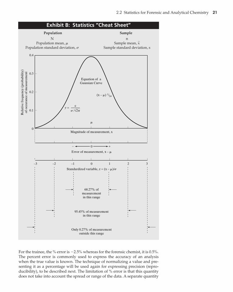
Population Sample

N nPopulation mean, Sample mean,

Population standard deviation, Sample standard deviation, ss

xm

Exhibit B: Statistics “Cheat Sheet”

0

0.1

0.2

0.3

0.4

�

Equation of aGaussian Curve

Rel

ativ

e fr

eque

ncy

(pro

babi

lity)

of o

ccur

ance

of m

easu

rem

ent

y =

Magnitude of measurement, x

0– +

Error of measurement, x – �

Standardized variable, z = (x – �)/�

68.27% ofmeasurementin this range

95.45% of measurementin this range

Only 0.27% of measurementoutside this range

� /√2�

e

(x – �) z/2�

0–1–2–3 321

For the trainee, the % error is whereas for the forensic chemist, it is 0.5%.The percent error is commonly used to express the accuracy of an analysiswhen the true value is known. The technique of normalizing a value and pre-senting it as a percentage will be used again for expressing precision (repro-ducibility), to be described next. The limitation of % error is that this quantitydoes not take into account the spread or range of the data. A separate quantity

-2.5%



0.4

0.3

–�A

–2�A

�B

–2�B +2�B

�B

+�A

+2�A

A

B0.2

0.1

0

Deviation from mean, x – �

Rel

ativ

e fr

eque

ncy

0 +–

� Figure 2.6 Two Gaussiandistributions centered aboutthe same mean, but with a dif-ferent spread (standard devia-tion). This approximates thesituation with the forensicchemist and the trainee.

†Although is based on sampling the entire population, it is sometimes used in forensic and ana-lytical chemistry. One rule of thumb is that if population statistics may be used. Similarly,if all samples in a population are analyzed, population statistics are appropriate. For example, todetermine the average value of coins in a jar full of change, every coin could be included in thesampling and population statistics would be appropriate.

n 7 15,s

is used to characterize the reproducibility (spread) and to incorporate it intothe evaluation of experimental results.

Standard deviation: The standard deviation is the average deviation fromthe mean and measures the spread of the data. (See Figure 2.6.) The standarddeviation is typically rounded to two significant figures. A small standard de-viation means that the replicate measurements are close to each other; a largestandard deviation means that they are spread out over a larger range of val-ues. In terms of the normal distribution, standard deviation from the meanincludes approximately 68% of the observations, standard deviations in-cludes about 95%, and standard deviations includes around 99%. A largevalue for the standard deviation means that the distribution is wide; a smallvalue for the standard deviation means that the distribution is narrow. The small-er the standard deviation, the closer is the grouping and the smaller is the spread.In other words, the standard deviation measures reproducibility of the measure-ments. The experienced supervisor produced data with more precision (less ofa spread) than that produced by the trainee, as would be expected based ontheir skill levels.

In Figure 2.5, two values are reported for the standard deviation: that ofthe population and that of the sample (s). The population standard devia-tion is calculated as

(2.3)

where i is the number of replicates, 10 in this case.† Ten replicates is a relativelysmall number compared with 100, 1000, or an infinite number, as would be re-quired to obtain the true value The value is the standard deviation of theparent population. The use of with small sample sets underestimates the truestandard deviation A statistically better estimate of is given by:

(2.4)

The value of s is the standard deviation of the selected subset of the parentpopulation. Some calculators and spreadsheet programs differentiate betweens and so it is important to make sure that the correct formula is applied.

The sample standard deviation(s) provides an empirical measure of uncer-tainty (i.e., expected error) and is frequently used for that purpose. If a distri-bution is normal, 68.3% of the values will fall between standard deviation

95.4% within 2s, and 99.7% within from the mean. This concept isshown in Figure 2.7. This spread provides a range of measurements as well asa probability of occurrence. Most often, the uncertainty is cited as standarddeviations, since approximately 95% of the area under the normal distributioncurve is contained within these boundaries. Sometimes standard deviationsare used, to account for more than 99% of the area under the curve. Thus, if the

;3

;2

;3s1;1s2, ;1

s,

s = San

i=1axi - xb2

n - 1

ss.2s

sm.

s = SaN

i=11xi - m22

n

1s2

;3;2

;1

1



distribution of replicate measurements is normal and a representative sampleof the larger population has been selected, the standard deviation can be usedto reliably estimate an uncertainty.

As shown in Table 2.1, the supervisor and the trainee both obtained a meanvalue within of the true value. When uncertainties associated with thestandard deviation and the analyses are considered, it becomes clear that bothobtained an acceptable result. This is also seen graphically in Figure 2.8. How-ever, the trainee would likely be asked to practice and try again, not because of

;0.3%

0.5a.

y

x

y

x

y

0.4

0.3

0.2

0.1

0.683

0– 4 – 3 – 2 – 1 0 1 2 3 4

0.5c.

0.4

0.3

0.2

0.1

0.997

0– 4 – 3 – 2 – 1 0

x1 2 3 4

0.5b.

0.4

0.3

0.2

0.1

0.954

0– 4 – 3 – 2 – 1 0 1 2 3 4

Figure 2.7 Area under theGaussian curve as a function ofstandard deviations from themean. Within one standarddeviation (a), 68.3% of themeasurements are found;95.4% (b) are found withintwo standard deviations, and(c) 99.7% are found withinthree standard deviations.

�



the poor accuracy, but because of the poor reproducibility. In any laboratoryanalysis, two criteria must be considered: accuracy (how close the result is tothe true value) and precision (how reproducible the result is). One without theother is an incomplete description.

Variance (v): The sample variance (v) of a set of replicates is simply which, like the standard deviation, gauges the spread, expected error, or vari-ance within that data set. Forensic chemists favor standard deviation as theirprimary measure of reproducibility, but variance is used in analysis-of-variance(ANOVA) procedures as well as in multivariate statistics. Variances are addi-tive and are the basis of error propagation, as seen in equation (2.1), where thevariance was represented by

%RSD of coefficient of variation (CV or %CV): The standard deviationalone means little and doesn’t reflect the relative or comparative spread of thedata. This situation is analogous to that seen with the quantity of absolute error.To compare the spread (reproducibility) of one data set with another, the meanmust be taken into account. If the mean of the data is 500 and the standard devi-ation is 100, that’s a relatively large standard deviation. By contrast, if the mean ofthe data is 1,000,000, a standard deviation of 100 is relatively tiny. The significance

e 2.

s2,

Min–Max 11.5–15.0 13.1–13.712.0–13.8 13.1–13.411.0–14.8 12.9–13.710.1–15.7 12.7–13.9

95% CI 12.2–13.6 13.2–13.4;3s;2s;1s

Table 2.1 Comparison of Ranges for Determination of PercentCocaine in QA Sample, m = 13.2%

Calculation Method Trainee, Forensic Chemist, x = 13.3x = 12.9

Trainee

Supervisor

11.0 Sample 12.0 12.8 13.0 13.4 13.6 14.0 15.0

95% CI

1S

Absolute error = � – x–

Absolute error = � – x–

+/– 3S

+/– 1S

+/– 3S

+/– 2S

95% CI

Figure 2.8 Results of thecocaine analysis presentedgraphically with uncertaintyreported several ways.

�



of a standard deviation is expressed by the percent relative standard deviation(%RSD), also called the coefficient of variation (CV) or the percent CV:

(2.5)

In the first example, or 20%; in the second,or 0.01%. Thus, the spread of the data in the

first example is much greater than that in the second, even though the values ofthe standard deviation are the same. The %RSD is usually reported to one or atmost two decimal places, even though the rules of rounding may allow more tobe kept. This is because %RSD is used comparatively and the value is not thebasis of any further calculation. The amount of useful information provided byreporting a %RSD of 4.521% can usually be expressed just as well by 4.5%.

%RSD = 1100/1,000,0002 * 100,%RSD = 1100/5002 * 100,

%RSD = 1standard deviation/mean2 * 100

Example Problem 2.2

As part of a method-validation study, three forensic chemists each made 10 replicateinjections in a GCMS experiment and obtained the following data for area counts of areference peak:

Injection No. A B C

1 9995 10640 98142 10035 10118 109583 10968 10267 102854 10035 10873 109155 10376 10204 102196 10845 10593 104427 10044 10019 107528 9914 10372 102119 9948 10035 10676

10 10316 10959 10057

Which chemist had the most reproducible injection technique?

Answer: This problem provides an opportunity to discuss the use of spreadsheets—specifically, Microsoft Excel®. The calculation could be done by hand or on a calcula-tor, but a spreadsheet method provides more flexibility and less tedium.

Reproducibility can be gauged by the %RSD for each data set. The data were en-tered into a spreadsheet, and built-in functions were used for the mean and standarddeviation (sample). The formula for %RSD was created by dividing the quantity inthe standard deviation cell by the quantity in the mean cell and multiplying by 100.

Injection #

12345678910

MeanStandard deviation %RSD

A B C

999510035109681003510376108451004499149948

10316

10640101181026710873102041059310019103721003510959

9814109581028510915102191044210752102111067610057

10247.6 379.14

3.70

10408.0 340.79

3.27

10432.9 381.57

3.66

Function used: = average()Function used: = stdev()mean/stdev*100



95% Confidence interval (95%CI): In most forensic analyses, there will bethree or fewer replicates per sample, not enough for standard deviation to be areliable expression of uncertainty. Even the 10 samples used in the foregoingexamples represent a tiny subset of the population of measurements that couldhave been taken. One way to account for a small number of samples is to applya multiplier called the Student’s t-value as follows:

(2.6)

where t is obtained from a table such as Table 2.2. Here, the quantity is the

measure of uncertainty as an average over n measurements.The value for t is selected on the basis of the number of degrees of freedom and the level of con-fidence desired. In forensic and analytical applications, 95% is often chosenand the result is reported as a range about the mean:

(2.7)

For the trainee’s data in the cocaine analysis example, results are best reportedas or Rephrased, the results can be expressed asthe statement that the trainee can be 95% confident that the true value lieswithin the reported range. Note that both the trainee and the supervisor ob-tained a range that includes the true value for the percent cocaine in the testsample. Higher confidence intervals can be selected, but not without due con-sideration. As certainty increases, so does the size of the range. Analytical andforensic chemists generally use 95% because it is a reasonable compromise be-tween certainty and range size. The percentage is not a measure of quality,only of certainty. Increasing the certainty actually decreases the utility of thedata, a point that cannot be overemphasized.

3

1m212.2–13.6195%CI2.12.9 ; 0.7,

X ;

s*t2n

s2n

confidence interval = x ;

s * t2n

1 6.314 12.706 63.6572 2.920 4.303 9.9253 2.353 3.182 5.8414 2.132 2.776 4.6045 2.015 2.571 4.032

10 1.812 2.228 3.169

Table 2.2 Student’s t-Values (Abbreviated); See Appendix 10 forComplete Table

90% confidence level 95% 99%n - 1

Analyst B produced data with the lowest %RSD and had the best reproducibility.Note that significant-figure conventions must be addressed when a spreadsheet isused just as surely as they must be addressed with a calculator.



2.2.2 OUTLIERS AND STATISTICAL TESTS

The identification and removal of outliers is dangerous, given that the onlybasis for rejecting one is often a hunch. A suspected outlier has a value that“looks wrong” or “seems wrong,” to use the wording heard in laboratories. Be-cause analytical chemists have an intuitive idea of what an outlier is, the sub-ject presents an opportunity to discuss statistical hypothesis testing, one of themost valuable and often-overlooked tools available to the forensic practitioner.The outlier issue can be phrased as a question: Is the data point that “looksfunny” a true outlier? The question can also be phrased as a hypothesis: Thepoint is (is not) an outlier. When the hypothesis form is used, hypothesis test-ing can be applied and a “hunch” becomes quantitative.

Suppose the supervisor and the trainee in the cocaine example both ran oneextra analysis independently under the same conditions and obtained a concen-tration of 11.0% cocaine. Is that datum suspect for either of them, neither of them,or both of them? Should they include it in a recalculation of their means andranges? This question can be tested by assuming a normal distribution of thedata. As shown in Figure 2.9, the trainee’s data has a much larger spread thanthat of the supervising chemist, but is the spread wide enough to accommodatethe value 11.0%? Or is this value too far out of the normally expected distribu-tion? Recall that 5% of the data in any normally distributed population will be onthe outer edges far removed from the mean—that is expected. Just because anoccurrence is rare does not mean that it is unexpected. After all, people do winthe lottery. These are the considerations the chemists must balance in decidingwhether the 11.0% value is a true outlier or a rare, but not unexpected, result.

To apply a significance test, a hypothesis must be clearly stated and musthave a quantity with a calculated probability associated with it. This is the fun-damental difference between a hunch† and a hypothesis test—a quantity and aprobability. The hypothesis will be accepted or rejected on the basis of a com-parison of the calculated quantity with a table of values relating to a normaldistribution. As with the confidence interval, the analyst selects an associatedlevel of certainty, typically 95%. The starting hypothesis takes the form of thenull hypothesis “Null” means “none,” and the null hypothesis is stated insuch a way as to say that there is no difference between the calculated quantityand the expected quantity, save that attributable to normal random error. As re-gards to the outlier in question, the null hypothesis for the chemist and thetrainee states that the 11.0% value is not an outlier and that any difference

H0.

3

3

Suppose a forensic chemist is needed in court immediately and must be located. Tobe 50% confident, the “range” of locations could be stated as the forensic laboratorycomplex. To be more confident of finding the chemist, the range could be extended toinclude the laboratory, a courtroom, a crime scene, or anywhere between any of thesepoints. To bump the probability to 95%, the chemist’s home, commuting route, andfavorite lunch spot could be added. To make the chemist’s location even more likely,the chemist is in the state, perhaps with 98% confidence. Finally, there is a 99% chancethat the chemist is in the United States and a 99.999999999% certainty that he or she ison planet Earth. Having a high degree of confidence doesn’t make the data “better”:Knowing that the chemist is on planet Earth makes such a large range useless.

Exhibit C: Is Bigger Better?

†Remove the sugarcoating and a hunch is a guess. It may hold up under quantitative scrutiny, butuntil it does, it should not be glamorized.



Trainee

a.

b.

Supervisor

Supervisor

11.0 12.0 12.8 13.0 13.4 13.6 14.0 15.0

95% CI

1S

Outlier ?

Outlier ?

Outlier ?

+/– 3S

+/– 1S

+/– 3S

+/– 2S

95% CI

13.311.0

Trainee

Supervisor

Trainee

Outlier ?Figure 2.9 On the basis ofthe spread seen for each ana-lyst, is 11.0% a reasonablevalue for the concentration ofcocaine?

�



between the calculated and expected value can be attributed to normal randomerror. Both want to be 95% certain that retention or rejection of the data is justi-fiable. Another way to state this is to say that the result is or is not significant atthe 0.05 ( or ), or 5% level. If the calculated value exceeds thevalue in the table, there is only a 1 in 20 chance that rejecting the point is incor-rect and that it really was legitimate based on the spread of the data.

With the hypothesis and confidence level selected, the next step is to applythe chosen test. For outliers, one test used (perhaps even abused) in analyticalchemistry is the Q or Dixon test:

(2.8)

To apply the test, the analysts would organize their results in ascending order,including the point in question. The gap is the difference between that pointand the next closest one, and the range is the spread from low to high, also in-cluding the data point in question. The table used (see Appendix 10) is that forthe Dixon’s Q parameter, two tailed. † If the data point can berejected with 95% confidence. The for this calculation with is0.444. The calculations for each tester are shown in Table 2.3. The results are notsurprising, given the spread of the chemist’s data relative to that of the trainee.The trainee would have to include the value 11.0 and recalculate the mean,standard deviation, and other quantities associated with the analysis.

In the realm of statistical significance testing, there are typically severaltests for each type of hypothesis.4 The Grubbs test, recommended by the Inter-national Standards Organization (ISO) and the American Society for Testingand Materials (ASTM),2,5,6 is another approach to the identification of outliers:

(2.9)

Analogously to obtaining Dixon’s Q parameter, one defines calculates G,and compares it with an entry in a table. (See Appendix 10.) The quantity G is theratio Z that is used to normalize data sets in units of variation from the mean.

H0,

G = ƒquestioned - x ƒ/s

n = 11Qtable

Qcalc 7 Qtable,3,

Qcalc = ƒgap/range ƒ

3

a = 0.05p = 0.05

Q test

Grubbs test Critical Z =

�13.3 - 11.0 �0.20

= 11.5Z =

�12.9 - 11.0 �0.93

= 2.04Z = 2.34

Qcalc =

[13.1 - 11.0][13.7 - 11.0]

= 0.778Qcalc =

[11.5 - 11.0][13.3 - 11.0]

= 0.217Qtable = 0.444

Table 2.3 Outlier Tests for 11.0% Analytical Results

Test Trainee Chemist

†Many significance tests have two associated tables: one with one-tailed values, the other withtwo-tailed values. Two-tailed values are used unless there is reason to expect deviation in only onedirection. For example, if a new method is developed to quantitate cocaine, and a significance testis used to evaluate that method, then two-tailed values are needed because the new test could pro-duce higher or lower values. One-tailed values would be appropriate if the method were alwaysgoing to produce, for example, higher concentrations.



range

Dixon Test (eq. 2.8)

(59.6 – 58.4)gap

(59.6 – 56.8)=Q = = 0.429

Table value = 0.477

Qcalc < Qtable = keep

Grubbs Test (eq. 2.9)

(59.6 – 57.53)0.8642

G = = 2.39

Table value (5%) = 2.176

Gcalc > Gtable = reject

Example Problem 2.3

A forensic chemist performed a blind-test sample with high-performance liquid chro-matography (HPLC) to determine the concentration of the explosive RDX in a per-formance test mix. Her results are as follows:

Laboratory data

56.8 57.257.0 57.257.0 57.857.1 58.457.2 59.6

Are there any outliers in these data at the 5% level (95% confidence)? Take any suchoutliers into account if necessary, and report the mean, %RSD, and 95% confidence in-terval for the results.

Answer: For outlier testing, the data are sorted in order such that the identifier iseasily located. Here, the questionable value is the last one: 59.6 ppb. It seems far re-moved from the others, but can it be removed from the results? The first step is to de-termine the mean and standard deviation and then to apply the two outlier testsmentioned thus far in the text: the Dixon and Grubbs approaches.

Mean = 57.53 Standard deviation 1s2 = 0.8642 n = 10

This is an example of contradictory results, and in such cases, ASTM recommendsthat the Grubbs test take precedence. Accordingly, the point is retained and the statis-tical quantities remain as is. The 95% confidence interval is then calculated:

95% confidence interval

0.8642

10

tsx–

by Appendix 102.26

+/–√n

(2.26)(0.8642)x = 0.618– +/–

√10

57.5 0.6 or 56.9 – 58.1+/–



For example, one of the data points obtained by the trainee for the percent co-caine was 15.0. To express this as the normalized z value, we have

(2.10)

This value is 2.26s, or 2.26 standard deviations higher than the mean. A valueless than the mean would have a negative z, or negative displacement. By com-parison, the largest percentage obtained by the experienced forensic chemist,13.7%, is 2.00s greater than the mean. The Grubbs test is based on the knowl-edge that, in a normal distribution, only 5% of the values are found more than1.96 standard deviations from the mean.† For the 11.0% value obtained by thetrainee and the chemist, the results agree with the Q test; the trainee keeps thatvalue and the forensic chemist discards it. However, different significance testsoften produce different results, with one indicating that a certain value is anoutlier and another indicating that it is not. When in doubt, a good practice isto use the more conservative test. Absent other information, if one says to keepthe value and one says to discard it, the value should be kept. Finally, note thatthese tests are designed for the evaluation of a single outlier. When more thanone outlier is suspected, other tests are used but this situation is not common inforensic chemistry.

There is a cliché that “statistics lie” or that they can be manipulated to sup-port any position desired. Like any tool, statistics can be applied inappropri-ately, but that is not the fault of the tool. The previous example, in which bothanalysts obtained the same value on independent replicates, was carefully stat-ed. However, having both obtain the exact same concentration should at leastraise a question concerning the coincidence. Perhaps the calibration curve hasdeteriorated or the sample has degraded. The point is that the use of a statisti-cal test to eliminate data does not, and should not, take the place of laboratorycommon sense and analyst judgment. A data point that “looks funny” war-rants investigation and evaluation before anything else—chemistry before sta-tistics. One additional analysis might reveal evidence of new problems,particularly if a systematic problem is suspected. A more serious situation is di-agnosed if the new replicate shows no predictable behavior. If the new repli-cate falls within the expected range, rejection of the suspicious data point wasjustified both analytically and statistically.

2.2.3 COMPARISON OF DATA SETS

Another hypothesis test used in forensic chemistry is one that compares themeans of two data sets. In the supervisor–trainee example, the two chemistsare analyzing the same unknown, but obtain different means. The t-test ofmeans can be used to determine whether the difference of the means is signifi-cant. The t-value is the same as that used in equation 2-6 for determining confi-dence intervals. This makes sense; the goal of the t-test of means is to determinewhether the spread of two sets of data overlap sufficiently for one to concludethat they are or are not representative of the same population.

In the supervisor–trainee example, the null hypothesis could be stated as“ The mean obtained by the trainee is not significantly different than themean obtained by the supervisor at the 95% confidence level ” Stat-ed another way, the means are the same and any difference between them isdue to small random errors.

1p = 0.052.H0:

6

z = 115.0 - 12.92/0.93 = 2.26

†The value standard deviations used previously is a common approximation of 1.96s.;2



The equation used to calculate the test statistic is

(2.11)

where the pooled standard deviation from the two data sets, is calcu-lated as

(2.12)spooled = Cs121n1 - 12 + s2

21n2 - 12n1 + n2 - 2

spooled,

tcalc =

|mean1 - mean2|spooled

A n1n2

n1 + n2

Example Problem 2.4

A toxicologist is tasked with testing two blood samples in a case of possible chronicarsenic poisoning. The first sample was taken a week before the second. The toxicolo-gist analyzed each sample five times and obtained the data shown in the accompany-ing figure. Is there a statistically significant increase in the blood arsenicconcentration? Use a 95% confidence level.

MeanVarianceObservationsHypothesized mean differencedft StatP(T<=t) one-tailt Critical one-tailP(T<=t) two-tailt Critical two-tail

Null hypothesis that means are the same is accepted.

Possible arsenic poisoningQ: Has there been a statistically significantincrease in the arsenic concentration?

Use Tools → Data analysis → t test unequal variancep = 0.05, hypothesized mean = 0Output:

Excel

Week 1 Week 2

17.02 0.027

5 0 6

–4.37 0.00 1.94 0.00 2.45

17.38 0.007

5

Week 116.917.116.817.217.1

Week 217.417.317.317.517.4

t table:

tcal = 4.37

tcal << t table:

[As] ppbin blood

2.365

Answer: Manual calculations for the t-test are laborious and prone to error. Thebest way to work such problems is with Excel, as shown in the accompanying figure.The feature used is under “Data Analysis,” found in the “Tools” menu. This analysispack is provided with Excel, although it has to be installed as an add-in. (See Excelhelp for more information on installing it.)

Once the data are entered, the analysis is simple. Notice that it was assumed thatthe variances were different; if they had been closer to each other in value, an alterna-tive function, the t-test of means with equal variances, could have been used. Also,the t-statistic is an absolute value; the negative value appears when the larger meanis subtracted from the smaller. For this example, which is greater than

This means that the null hypothesis must be rejected and that the con-centration of arsenic has increased from the first week to the second.ttable = 2.365.

tcalc = 4.37,



This calculation can be done manually or preferably with a spreadsheet, asshown in Example Problem 2.4. The result for the supervisor/trainee is a of 1.36, which is less than the (Appendix 10) of 2.262 for 10 degrees of free-dom. Therefore, the null hypothesis is accepted and the means are the same atthe 95% confidence level or This is a good outcome since bothchemists were testing the same sample. Note that the t-test of means as shownis a quick test when two data sets are compared. However, when more datasets are involved, different approaches are called for (4,7).

2.2.4 TYPES OF ERROR

One other set of statistical terms merits mention here, as they are often used in aforensic context. Whenever a significance test is applied such that a null hy-pothesis is proposed and tested, the results are always tied to a level of certain-ty, 95% in the example in the previous section. With the forensic chemist’s data,the 11.0% data point was identified as an outlier with 95% certainty, but that stillleaves a 1-in-20 chance that this judgment is in error. This risk or possibility oferror can be expressed in terms of types. A Type I error is an error in which thenull hypothesis is incorrectly rejected, whereas a Type II error is an error inwhich the null hypothesis is incorrectly accepted. Put in terms of the experi-enced chemist and the 11.0% value, states that that value is not an outlier,but the null hypothesis was rejected on the basis of the calculations for the Qtest and the Grubbs test. If that were in fact a mistake, and the 1-in-20 long shotcame true, throwing out the 11.07%. value would be a Type I error. In effect, thechemist makes a defensible judgment in rejecting that value, deciding that theharm done by leaving it in would be greater than the risk of throwing it out.

2.2.5 SAMPLING STATISTICS

Overview: One important application of statistics in forensic chemistry is in theselection of a defensible and representative sample n from a larger parent popu-lation. Each type of exhibit generates a different sampling challenge, from thebarely detectable fragment of a synthetic fiber to the seizure of hundreds of pack-ets of white powder. Regardless of the nature of the evidence, foundational prin-ciples of representative sampling apply, with the forensic caveat that the evidenceshould not be totally consumed in testing unless that is absolutely unavoidable.By definition, a defensible and representative sample is a random sample. Itshould not matter how, when, or where a subset or aliquot is drawn for analysis.If it does, further preparation and sorting are called for before samples are taken.

Neither the forensic literature nor the courts have provided concrete rulesor definitions for what constitutes a representative sample. Partially this is dueto the nature of forensic samples, and partly it has to do with the lack of con-sistent legal standards. In general, the courts have emphasized the need forrandom and representative samples, but have not specified how those qualitiesare to be assured or quantified.8 This gap between what is needed and how tosatisfy that need should not be terribly surprising or troubling, given the infi-nite variety of evidence that enters forensic laboratories daily: In practicalterms, it is far easier to identify a poor sampling plan than create the perfectone. In recognition of this fact, the treatment that follows is a general discus-sion of representative sampling couched in terms just introduced: normal dis-tributions, probabilities, significance testing, and homogeneity.

If a sample is properly and thoroughly mixed, it will be homogeneous andthe composition of any portion of it will be representative. Analysts thoroughly

8,9

H0

p = 0.05.

ttable

tcalc



mix any sample before selecting an aliquot if such mixing is (1) applicable (onedoes not mix fibers purposely collected from different areas of a body), (2) pos-sible (it’s hard to mix a ton of green plant matter), and (3) appropriate (if sever-al baggies of powder are seized, some tan and some black, they should not bemixed). Deciding when these conditions are satisfied relies on analyst judg-ment and the particulars of the case. In the discussion that follows, it is as-sumed that the analyst will, if necessary, ensure that the final subset or aliquotis drawn from a properly and appropriately homogeneous sample.

Consider an example in which a forensic laboratory receives evidence from asingle case. Suppose the evidence consists of a hundred baggies, each full of whitepowder. Do all of the bags need to be tested, or can a representative subset suf-fice? A subset suffices if the powder in all of the bags is part of the same batch—instatistical terms, if all of the samples are part of the same population. So the foren-sic scientist has to answer the following question: Was some large shipment di-vided into these individual bags, or does this case represent several differentoriginal sources? In other words, does each of these n samples belong to a largerparent population that is normally distributed with respect to the variables of in-terest? If so, any difference between samples selected are due only to small ran-dom variations that would be expected of a normally distributed population. Thisargument should sound familiar; in a normally distributed population, there is a68% probability that a randomly selected sample will be within of the mean,a 95% probability that it will be between etc. Although one sample does notcompletely describe the distribution, it isn’t necessary to test all samples.

The previous paragraph is another window on the earlier sampling (n)versus parent population statistics discussion. The goal is to minimize the dif-ferences and and to be able to assign a level of certainty to theestimates. Selecting such a representative subset is called probability sam-pling or selecting an unbiased subset. When an unbiased subset is successfullychosen, n is a perfect snapshot of N. Designing a probability sampling plan ispart and parcel of quality assurance and data integrity, yet forensic laboratoriesalso have to balance cost and time considerations and allow room for analystjudgment. This is particularly true in drug analysis, the area of forensicchemistry that deals with sampling issues the most often. As of late 2004, inter-national forensic working groups such as the Scientific Working Group for theAnalysis of Seized Drugs (SWGDRUG, swgdrug.org) were working on samplingguidelines to be recommended to the forensic community. Forensic chemistsshould monitor the progress of these groups and their findings, as they will likelydefine future sampling practices. The remainder of this discussion utilizes druganalysis to exemplify the principles introduced, which are applicable to all areasof forensic chemistry in which sampling plans are needed.

5,10

ƒs - s ƒƒx - m ƒ

;2s,;1s

A AA

A

A ABBB B

N = 1000

Population = 600A400B

n = 10Sampling

Plan

A

A

A

AA A

A

A

A A

B

B B

BB

B

B B

B

Figure 2.10 Ideally, a subsetof n samples will capture thecomposition of the larger par-ent population.

�



Although the terms “statistics” and “probability” are often used interchangeably, theyrefer to different concepts. Statistics is based on an existing data set, such as that in thereplicate measurement example of the supervisor and trainee used throughout thischapter. Based on knowledge of random populations and the Gaussian distribution,patterns observed in the smaller data set are extrapolated to the overall population. Anexample is the use of the sample standard deviation s as a starting point for determin-ing a confidence interval. Thus, statistics is an inductive process wherein specificknowledge is extrapolated and applied generally. By contrast, probability is deductiveand moves from general knowledge to a specific application. Describing the probabili-ty that a coin toss will yield three tails starts with the general knowledge that any onecoin toss can give either a head or a tail. However, what statistics and probability dohave in common is that they both describe uncertainty. A coin-toss question can bephrased in terms of the odds; the odds that three coin tosses in a row will produce threetails is or 1 in 8, meaning that, given a fair toss, one can expect three tails orthree heads 1 time in 8, or 12.5% of the time. Nonetheless, that does not mean that if onereplicates the three-toss experiment eight times, it is assured that one sequence will bethree heads or three tails. There is still uncertainty associated with the outcome.

Source: Aitken, C. G. G., and F. Taroni. Statistics and the Evaluation of Evidence forForensic Scientists, 2d ed. Chichester, U.K.: John Wiley and Sons, 2004, p. 6.

11/223,

Exhibit D: Statistics and Probability

A Working Example: Suppose a large seizure of individual baggies of white powderhas arrived at the laboratory. Controlled substances in the powder are to

be identified and quantitated in an expeditious and cost-effective manner. Clearly, asampling plan is needed. The forensic literature and the standard (or at least com-mon) laboratory practices furnish a starting point for the design of such a plan, andan illustrative example is provided in Table 2.4. According to recent data, most lab-oratories appear to use the first two methods listed in the table or variations ofthem, combined with presumptive and screening tests. The latter phrase is animportant qualifier and will be discussed shortly. Note that the number of samplestested to completion is not the sole criterion for judging the merit of a samplingplan; as mentioned earlier, it is usually easier to judge a bad approach than dictatethe perfect one. Accordingly, there is nothing inherently wrong with a case-by-caseapproach to sampling; the key as always is to ensure that the plan is defensible.

11

1n = 1002

7 10 12(10%) 5 10 15(4%) 2 4 6

5 7 9

Hypergeometric distribution NA23 28 33

Note: total number of separate articles of evidence to be sampled; size of thesubset of samples. This table is based on one presented in Colon, et. al. “NA” means thatthe value was not provided in the reference directly.For a 95% certainty that 80–90% of the entire collection is positive; assumes no negatives inpresumptive testing.

*

11n = theN = the

20 + 0.101N - 20225*12*

AN2

N * 0.04N * 0.102N

Table 2.4 Comparison of Methods Used for Determining n

Formula for Determining n N = 150, n = ?N = 100, n = ?N = 50, n = ?



An essential first step in sampling is visual inspection. Are the samples allthe same color? Do they have the same granularity? If so, a hypothesis can beput forward that all of the samples are from the same batch or population andthat any variation found within them is small and the result of an expected nor-mal distribution. Next, a battery of presumptive tests or screening tests could beapplied to each sample. Presumptive testing is described in detail in Chapter 7;suffice it for now to say that a positive result issuing from a screening test indi-cates that the substance is more likely than not to contain what it is suspected tocontain. Suppose in this example that the screening tests all pointed to an iden-tification of cocaine with similar characteristics, adding further confidence tothe hypothesis that all the bags are part of the same population. Had either thevisual or screening tests failed to support this assumption, the samples wouldthen be placed into similar groups, each representing a new population.

The next step is the selection of n, the subset of the 100 exhibits that will ad-equately characterize the population with acceptable error (also called tolera-ble error) and acceptable uncertainty. Some methods available for selecting nare as follows:

ASTM E122-05: This protocol is designed for articles within a batch or lot, a rea-sonable model for the hypothetical drug seizure. The equation used is

(2.13)

where e is the tolerable error and is the estimated standard deviation of thepopulation. Since making such an estimate is somewhat difficult, an alterna-tive based on the percent RSD expected or desired is

(2.14)

where is the CV (%RSD) and e is the allowable error, also expressed as aratio or percentage. For our hypothetical case introduced above, assume thatan error of 2% is acceptable and a %RSD of 5% is expected, onthe basis of the laboratory’s previous experience. Then

(2.15)

If only the average value of a lot or batch is needed, the value of n can be fur-ther reduced with the use of the formula

(2.16)

where refers to the size of a lot or batch.

Normal Distribution: Another approach to selecting a subset is based on theassumption that variation in the subset is normally distributed. If so, then thesampling question can be rephrased to facilitate the selection of a reasonablysized subset n of a larger population N based on expectations or suspicions re-garding how many items in the seizure are cocaine. Suppose that 72 of the12

12

nL

nL =

n

c1 + a nNb d

=

56

c1 + a 56100b d

= 35.897 = 36

n = a3 * 52b2

= 56.25 = 56

1V0 = 521e = 22V0

n = a3V0

eb2

s0

n = a3s0

eb2



baggies of powder contain cocaine and 18 do not. Then the value defined as is 72/100, or 0.72. Of course, the analyst does not know this prior to testing;rather, the goal is to select a random subset that provides an unbiased estimateof This unbiased proportion can be represented as p = z /m, where m is thesize of the subset chosen and z is as defined in equation 2.10.12 On the basis ofprevious experience, the analyst expects the seizure to contain approximately75% cocaine exhibits and the rest noncontrolled substances. The analyst’s goal isto estimate the ratio of cocaine to substances that are not cocaine to within On the basis of the normal distribution, one expression that can be used is

(2.17)

In addition to assuming a normal distribution, this expression relies on the as-sumption that the selected subset’s ratio of cocaine will lie somewhere between

at a 95% confidence level. The analyst then would select 12 sam-ples and analyze them. The results would allow the analyst to state with 95%confidence that the proportion of cocaine to substances that are not cocaine inthe seizure is indeed greater than 50%. Why 50% and not 75%? The 50% figurearises from the range selected: Equation 2.17 can be useful for ini-tial estimates, but a more flexible approach is one based on probabilities.

Hypergeometric Distribution and Related Techniques The hypergeometricprobability distribution is used in situations where samples are to be takenfrom a large population and not replaced. Consider a deck of cards, an exam-ple of a finite population. If 10 cards are drawn at random (and not replaced inthe deck), a hypergeometric distribution could be employed to calculate theprobability of drawing four queens in the 10 cards drawn. The hypergeometricmean is related to the binomial distribution used in forensic DNA analysis tocalculate gene frequencies, and it applies to cases in which the outcome can beonly one of two options. Flipping a coin is the classic example. To calculate theprobability of getting 3 heads in a row, the individual probabilities are multi-plied This figure can be expressed as approximately a13% chance that three coin flips will produce 3 heads. The probability of getting10 in a row is much smaller, namely 0.001, which can be stated as 1 chance in1024. In the example of the bags of cocaine, the selection of any one bag can beconsidered an exclusive or (either/or) option—either it will contain cocaine orit will not. This is the reasoning behind the application of the binomial and hy-pergeometric distributions to selective sampling.

0.5 * 0.5 * 0.5 = 0.125.

9, 12–14:

0.75 ; 0.25.

0.75 ; 0.25

m =

4u11 - u20.252 =

4 * 0.7511 - 0.7520.252 = 12

12;25%.

u.

u

The American Society for Testing and Materials, now known as ASTM International,was formed in 1898 to provide uniform standards for testing procedures used in sci-ence and engineering. The first “standard” (actually a written protocol), was calledA-1 and covered stainless steel. The person most responsible for the founding ofASTM was the American Charles B. Dudley, a Ph.D. chemist. Over the years, ASTMformed committees and generated standards for many industries. ASTM’s standardsare based on consensus in that they are written by committees of practitioners in theappropriate field. Committee E-30, which concerned itself with forensic science, wasformed in 1970; several of its standards are referenced in this text. ASTM publishesthe Journal of Forensic Sciences.

Historical Evidence 2.1—ASTM International



Example Problem 2.5

A seizure of 369-kilo bricks of a tan powder is received in a crime laboratory. All ofthe bricks are carefully weighed, and it is determined that all weigh

The prosecuting attorney explains to the analyst that the penalty ismore severe if controlled substances are found in the amount of more than 100.0 kg.Using the hypergeometric-mean approach, devise a reasonable sampling plan.

Answer: Enough samples must be tested to be sure that the amount of controlledsubstance found, if any, conclusively exceeds or does not exceed the 100.0-kg thresh-old. First, take into account the uncertainties of the weights. The worst possible casewould be if every brick selected had a low weight. If so, more would have to be sam-pled to ensure that if all were found to contain the same controlled substance, theweight exceeded 100 kg. The determinative equation is

Accordingly, to ensure that the weight threshold is exceeded, at least 101 of the bricksmust be found to contain the same controlled substance. By contrast,

bricks must be shown to contain no controlled substance in order toensure that the threshold is not exceeded.

The Excel hypergeometric-mean function was used to generate the following table:

Initial random No. positives Population sample observed positives % chance Odds: 1 in

10 10 10 8.77E-1810 10 25 2.87E-1110 10 50 9.01E-0810 10 75 7.27E-0610 10 101 1.68E-0410 10 150 1.03E-0210 10 200 0.2 508.010 10 250 1.9 52.110 10 260 2.9 34.910 10 270 4.2 23.810 10 280 6.1 16.410 10 300 12.3 8.210 10 350 58.5 1.710 10 360 77.9 1.310 10 368 97.3 1.0

Here it is assumed that the analyst decided to take 10 samples at random and testthem completely. Suppose all came back positive for a controlled substance and werethe same as far as the analysis showed. What are the odds that at least 101 would thenbe positive? The first line of the table shows that if there were 10 positives in the en-tire population of 369 kilos, the odds of selecting those 10 at random are on the orderof 1 in At the other extreme, if 360 of the 369 are positives, there is nearly an 80%chance that the first 10 selected at random will test positive. Assume that 101 are posi-tive. If 10 samples are drawn from the entire 369 at random and are then found posi-tive, that would be expected to occur only once in approximately 10,000 tries.

What does the latter statement mean for the analyst? If he or she samples 10, ana-lyzes them, and finds that all are positive, then there is only 1 chance in 10,000 thatless than 101 kilos contain the controlled substance. The advantage of using thespreadsheet function is that it allows for a “what if?” approach. Once the formulas areset up, the values for the initial random sample and other variables can be adjusted inaccordance with different scenarios.

1019.

9.75E + 035.94E � 051.38E + 071.11E + 093.49E + 121.14E + 19

Á

369 - 101 = 268

100.0 kg/0.995 kg = 100.53

1.00 kg ; 0.05 kg.



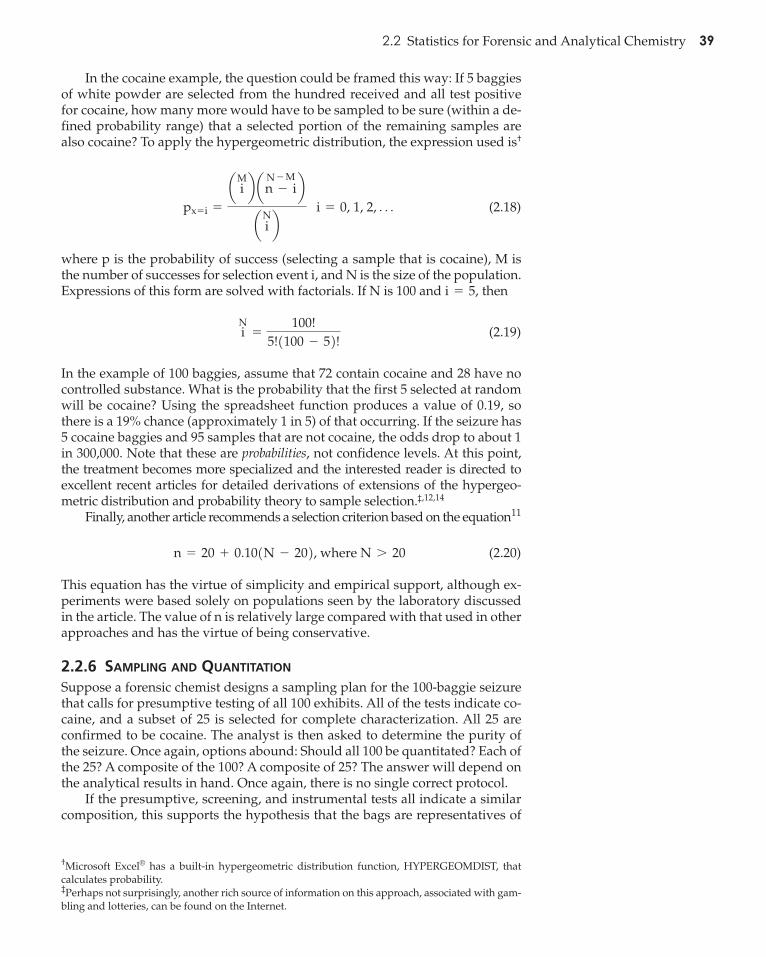
In the cocaine example, the question could be framed this way: If 5 baggiesof white powder are selected from the hundred received and all test positivefor cocaine, how many more would have to be sampled to be sure (within a de-fined probability range) that a selected portion of the remaining samples arealso cocaine? To apply the hypergeometric distribution, the expression used is†

(2.18)

where p is the probability of success (selecting a sample that is cocaine), M isthe number of successes for selection event i, and N is the size of the population.Expressions of this form are solved with factorials. If N is 100 and then

(2.19)

In the example of 100 baggies, assume that 72 contain cocaine and 28 have nocontrolled substance. What is the probability that the first 5 selected at randomwill be cocaine? Using the spreadsheet function produces a value of 0.19, sothere is a 19% chance (approximately 1 in 5) of that occurring. If the seizure has5 cocaine baggies and 95 samples that are not cocaine, the odds drop to about 1in 300,000. Note that these are probabilities, not confidence levels. At this point,the treatment becomes more specialized and the interested reader is directed toexcellent recent articles for detailed derivations of extensions of the hypergeo-metric distribution and probability theory to sample selection.‡

Finally, another article recommends a selection criterion based on the equation

(2.20)

This equation has the virtue of simplicity and empirical support, although ex-periments were based solely on populations seen by the laboratory discussedin the article. The value of n is relatively large compared with that used in otherapproaches and has the virtue of being conservative.

2.2.6 SAMPLING AND QUANTITATION

Suppose a forensic chemist designs a sampling plan for the 100-baggie seizurethat calls for presumptive testing of all 100 exhibits. All of the tests indicate co-caine, and a subset of 25 is selected for complete characterization. All 25 areconfirmed to be cocaine. The analyst is then asked to determine the purity ofthe seizure. Once again, options abound: Should all 100 be quantitated? Each ofthe 25? A composite of the 100? A composite of 25? The answer will depend onthe analytical results in hand. Once again, there is no single correct protocol.

If the presumptive, screening, and instrumental tests all indicate a similarcomposition, this supports the hypothesis that the bags are representatives of

n = 20 + 0.101N - 202, where N 7 20

11

,12,14

iN

=

100!5!1100 - 52!

i = 5,

px= i =

a iMb an - i

N - M ba i

Nb i = 0, 1, 2, Á

†Microsoft Excel® has a built-in hypergeometric distribution function, HYPERGEOMDIST, thatcalculates probability.‡Perhaps not surprisingly, another rich source of information on this approach, associated with gam-bling and lotteries, can be found on the Internet.



the sample population. If differences in composition are noted, then the sam-ples should first be grouped. Perhaps half of the samples analyzed were cutwith caffeine and half with procaine. All contain cocaine, but clearly two sub-populations exist and they should be treated separately.

Recall that the standard deviation is an expression of precision but that it isnot additive. Variance, however, is additive and can be used as a starting pointfor devising a plan for quantitation. The overall uncertainty in quantitativedata will depend on two categories of uncertainty: that which arises from theanalytical procedure and that which is inherent to the sample

(2.21)

Given that methods used in a forensic laboratory will be validated and opti-mized, it is reasonable to assume that in most cases, the variance contributedby the analytical method will be significantly smaller than the variation arisingfrom sampling. Thus, in most cases, can be ignored. The goal of a samplingplan for quantitative analysis is to reduce the overall variance by reducing thesampling variance and confining it to acceptable ranges. The absolute error inany mean percent cocaine calculated from sampling several items can be ex-pressed as the true value minus the calculated mean, or

(2.22)

where e is the desired absolute error in the final result and t is obtained from theStudent’s t-table on the basis of the confidence level desired. Solving for n yields

(2.23)

In most cases, the difficulty is estimating If the initial assumption (that allsamples are essentially the same or homogeneous) is correct, a smaller valuewould make sense; if appearance or other factors call this assumption intoquestion, a larger value of would be needed. Returning to the 100-baggiecase, if a quantitative absolute error e of 5% is acceptable and a standard devi-ation of 7% is anticipated, the number of samples needed to obtain a mean with

Ss

Ss.

n =

t2ss2

e2

m - x =

tss2n or e =

tss2n

m

Sa

ST2

= Ss2

+ Sa2

1Ss2:1Sa2ST

Alphonse Bertillon (French, 1853–1914), a pioneer in forensic science, was involved inan early case that employed probability-based arguments. Alfred Dreyfus was aFrench officer accused of selling military secrets. A document he admitted writingwas seized as evidence against him. Using a grid, Bertillon analyzed the documentand determined that 4 polysyllabic words out of 26 were positioned identically rela-tive to the grid lines. Bertillon argued that such coincidence of positioning was high-ly unlikely with normal handwriting. Arguments were also made concerning thenormal frequency of occurrence of letters in typical French versus those found in thequestioned document. Subsequent analysis of the case and testimony showed thatBertillon’s arguments were incorrect.

Source: Aitken, C. G. G., and F. Taroni. Statistics and the Evaluation of Evidence for Foren-sic Scientists, 2d ed. Chichester, U.K.: John Wiley and Sons, 2004, Section 4.2.

Historical Evidence 2.2— The Dreyfus Case



a 95% CI would be calculated iteratively, starting with the assumption that thenumber of degrees of freedom is infinite:

Now, the actual number of degrees of freedom is 6, and the calculation is re-peated with the new value of t:

The process continues until the solution converges on Notice that thenumber of pieces of evidence in the seizure (size of the larger parent popula-tion) is never given. The only consideration is the variance among the individ-ual pieces. The weakness of the procedure is the estimation of but analystexperience can assist in such cases. This approach can also be used to select thesize of a representative subset for sampling.

2.2.7 BAYESIAN STATISTICS

This topic is a proverbial hot potato in the forensic community. Whether oneagrees or disagrees with how it has been applied, it hurts nothing to be familiarwith it.† This section is meant only to provide a brief overview of a Bayesianapproach to sampling statistics. For more information, Aitken’s book (see “Fur-ther Reading” section at end of chapter) is highly recommended. Bayesian statis-tics formally and quantitatively incorporates prior knowledge into calculationsof probability. This feature was touched upon in the 100-baggie example, inwhich the analyst used experience with similar cases to estimate the ratio of ex-hibits likely to contain cocaine to the total number of bags seized (ratio ex-pressed as ). Bayesian statistics can and has been used in many areas offorensic science and forensic chemistry, including sample selection and analy-sis. The controversy over its use centers on whether the introduction of analystjudgment is subjective rather than objective. As will be seen, applied with duecare and thought, this method becomes another valuable tool with strengthsand weaknesses akin to those of any other instrument.

The Bayesian approach is a logical addition to the hypergeometric distri-bution and binomial distribution techniques introduced earlier. The idea be-hind the hypergeometric distribution is that, in a finite population such as adeck of cards or a drug seizure, a probability can be assigned to test results ifthere is knowledge of the possible outcomes. For a large drug seizure of N sam-ples, a subset n can be removed and tested. For each test, the result is eitherpositive or negative, so a fraction of positives in the subset can be calculated asm/n where m is the number of positives. A probability can then be assigned tothe proportion M/N of positives in the parent population. This approachechoes the point made earlier that the better the selection of the subset n, thebetter the composition of n represents the composition of the parent popula-tion. Bayes’s theorem can be invoked to rephrase this relationship in order toassist in selecting n and estimating M.14

14

u

Ss,

n = 10.

n =

2.447210.07220.052 L 12

n =

1.960210.07220.052 = 7.53 L 7

†As evidence of the depth of feeling on this topic, one text (K. Inman and N. Rudin, Principles andPractices of Criminalistics, (Boca Raton, FL: CRC Press, 2001)) warns readers that “this approachshould be viewed as a tool, not a religion” (p.143).



A Bayesian approach is based on a likelihood ratio that takes into accountinformation that the analyst supplies. A generalized form of this ratio is

(2.24)

where Pr denotes probability and is the hypothesis based on m. Althoughcomplicated, the expression essentially states that the probability of any onehypothesis being true depends on how likely that outcome is, given all otherpossible outcomes. Equation (2.24) can be solved with factorials or, more con-veniently, by the Excel function mentioned previously. With a set of hypothe-ses, the result is a set of probabilities that allow for the selection of a defensiblesample size m. The prior probability is the probability of the hy-pothesis being true for sample size N before analysis.

The article by Coulson, et al.,14 uses a spreadsheet to delve in detail into theimplementation of this approach and provides an example of 100 exhibits sim-ilar to our 100 baggies example. In the example from this report the analyst firsthypothesizes, on the basis of observation, that all exhibits are homogenous andrepresent the same population. That is, This means that allthe exhibits will be positive or all will be negative. From experience (priorknowledge or posterior knowledge), the analyst also hypothesizes that 60%will be positive, or If all of the exhibits were tested, therewould be 101 possible outcomes: 100 positive; 100 negative; and 99 combina-tions running from The method allows the probabilities ofeach of these outcomes to be calculated. If 5 exhibits are tested and are positive,the probability of all 100 being positive is 0.9973; if 50 are analyzed, the proba-bility increases to 0.9998.

99:1, 98:2, Á , 1:99.

Pr1pos ƒhom2 = 0.6.

Pr1hom2 = 0.99.

Pr1Hm ƒN2,

12

Hm

Pr1Hm|N, n, m2 =

Pr1m|Hm, n, M2Pr1Hm|N2aPr1m ƒHm, n, N2Pr1Hm ƒN2

14

Applying the Science 2.1 Sample Selection for Weighing

Source: Azoury, M., et al. “Evaluation of a Sampling Procedure for Heroin Street Doses.” Journal of Forensic Sciences, 431998, 1202–1207.

The weights of exhibits are an important issue in somecases, and in large seizures it may be impractical to weigheach sample, just as it is impractical to test all the samples.The problem is that total weights must be reported to a rea-sonable degree of certainty. In Israel, the solution has beenboth legislative and scientific. The law defines the samplingprotocol to be used, assuming that the samples all appearsimilar: According to this protocol, the sample size (n) fromthe total population (N) depends on the population size: 5of a population up to 15 units, 6 between 16 and 50 units,and 7 if the population exceeds 51 units. Each randomly se-lected sample is weighed on a balance that is linked to acomputer which calculates the mean S and a 95%CI for theweights, based on the weights of the random subset. Theacceptance criterion is

1.96 * 0.1x

* 100 L …15%

where 0.1 is the uncertainty expected for the mean weight.If the calculated value exceeds 15%, the analyst weighsmore exhibits until all are weighed or the acceptance crite-rion is satisfied. As an example, if the mean were 3.0 g andthe associated uncertainty at that weight were 0.3 g, the cal-culation would be or 19.6%. Ifthis were the case, the examiner would have to weigh moreexhibits.

To test the procedure, the laboratory evaluated approxi-mately 1500 seized units in different ways to compare the es-timated weights with the actual ones. The findings showedthat, for about 88% of the exhibits, the actual weight waswithin the 95% CI, and a potential bias in sampling proce-dure was noted. Original estimates were lower than the trueweight by approximately 0.7%, suggesting that the selectionof individual exhibits for n may not be completely randomor representative. The authors offered computerized ran-dom selection as a way to eliminate any analyst bias.

111.96 * 0.32/3.02 * 100,


Problems 43

SSUMMARUMMARYY

Statistics is a fundamental and quantitative component of quality assurance. Statistics isalso a powerful tool for the forensic chemist, in that it can describe the accuracy and pre-cision of data, assist in answering hypothesis-based questions, and identify trends andpatterns in data. Statistics and the related tools of probability can be applied to directsampling and provide a reasonable, defensible, and sensible sampling plan. With such aplan in hand, we are ready to move on to multivariate statistics, calibration, and the uni-fication of these concepts under the umbrella of quality assurance and quality control.

KKEYEY TTERMSERMS ANDAND CCONCEPTSONCEPTS

Quality controlTotal quality managementUncertaintySignificant figuresAbsolute uncertaintyRelative uncertaintyAbsolute errorVarianceStandard deviationMeanOutlier

Q testGrubbs testType I errorType II errorRepresentative sampleSampling statisticsHomogeneousBinomial distributionBayesian statisticsPopulationSignificance test

NormalizationDixon’s testz-transformPropagation of uncertaintyRelative errorHypothesisHypergeometric distributionGaussian curve/distributionBell curveSample size (N/n)Probability sampling

PPROBLEMSROBLEMS

From the chapter

1. A standard of for a gunshot residue analysis usingatomic absorption is prepared by first dissolving 1.0390 gdried in distilled water containing 1% nitricacid. The solution is brought to volume in a class-A500-mL volumetric flask with an uncertainty of

The solution is then diluted 1/10 by taking10 mL (via an Eppendorf pipet, tolerance ) anddiluting this in 1% nitric acid to a final volume of 100mL in a volumetric flask with a tolerance of The balance has an uncertainty of a. Using conventional rounding rules, calculate the

concentration of the final solution of in ppm.b. Determine the absolute and relative uncertainties of

each value obtained in part a. Select the largest andreport the results as a concentration range.

c. Report the results as a range by the propagation-of-error method.

d. Comment on your findings and why this case issomewhat unique.

2. If an outlier is on the low side of the mean, as in the ex-ample in the chapter, could a one-tailed table be used?

3. Find the following reference for Q value tables:Rorabacher, D. B. “Statistical Treatment for Rejection ofDeviant Values: Critical Values of Dixon’s ‘Q’ Parameter

Pb2+,

;0.0002 gram.;0.08 mL.

;1.3 mL;0.20 mL.

Pb1NO322Pb2+

and Related Subrange Ratios at the 95% ConfidenceLevel.” Analytical Chemistry, 63 1991, 139–148. For thetrainee/forensic chemist example used throughout thischapter, determine what the percent cocaine wouldhave to be in the 11th sample for it to be eliminated atthe following significance levels: 0.20, 0.10, 0.05, 0.04,0.02, and 0.01. Present your findings graphically andcomment on them.

4. Differentiate clearly between statistical and analyticalerrors.

5. Justify or explain the use of the factor 3 in equation 2.12.6. The results of equation 2.14 blatantly ignore significant-

figure conventions. Why?7. a. A large seizure containing 1500 individually pack-

aged units of a tan powder arrives at the laboratory.All units appear similar, and each weighs a kilo-gram. This is an unusual case unlike any seen beforein this facility, and the laboratory staff has neitherthe time nor the resources to test all 1500 units. De-sign a sampling plan for qualitative analysis basedon the methods described in the text. Summarize theoutcome and justify a final value of n. As appropri-ate, note any assumptions made.

b. The recommendation you made in part a is accepted,and the selected subset is tested and found to con-tain heroin, with all samples appearing to come from



the same batch. The federal prosecutor needs toknow the average percent heroin in the seizure withan accuracy of (relative) and a precision of

Design a sampling plan for quantitation anddefend the plan.

8. A small seizure consisting of 30 blotter papers of sus-pected LSD is submitted to the laboratory.a. Design a sampling plan, assuming that the contents

of a minimum of three papers will be needed to ob-tain a sample sufficient for presumptive and confir-matory testing.

b. After selecting n samples and testing them, you findthat all are negative. Describe the next steps in theanalysis.

c. At what point in this analysis would it be appropri-ate to call the results negative for LSD?

d. Assume that all samples tested are negative untilfour squares are left. Testing one gives a positive re-sult. Using a flowchart, describe the next step(s) andany assumptions made.

This problem will be seen again in a later chapter, whereadditional analytical information can be brought to bearon its solution.

9. An analyst proposes a new method for analyzing bloodalcohol. As part of a method validation study, she ana-lyzes a blind sample five times and obtains the follow-ing results: 0.055%, 0.054%, 0.055%, 0.052%, and 0.056%.a. Are there outliers in the data?b. On the basis of the results of the outlier analysis and

subsequent actions, calculate the mean and the%RSD of the analyst’s results.

c. If the true value of the blind sample is 0.053%(based on a range of ), is the mean

value obtained by the analyst the same as the truevalue at p = 0.05?

;2s;0.002%

;2%.;5%

Integrative

1. Use the Excel function for the hypergeometric distribu-tion to calculate the probability of selecting five samplesthat will be positive for cocaine if a seizure contains1000 baggies and past laboratory data suggest that 50%of such recent seizures are cocaine and the rest are not.Study the results and explain how the hypergeometricdistribution is similar to a simple binomial distribution.

2. What is the difference between a confidence level and aprobability?

3. A university instructs its professors to assign grades inthe range from 0.0 for an F to 4.0 for an The lettergrade is not recorded; only the number grade is. Whenstudents’ GPAs are calculated, they are reported to threedecimal places. Can this be justified by the rules of sig-nificant figures?

4. Are random samples representative by definition? Arerepresentative samples random by definition? Whatcondition must exist for each of these questions to beanswered affirmatively?

5. Why can there never be such a thing as a true value?6. A government agency, the National Institute of Stan-

dards and Technology (NIST), provides certified refer-ence materials to forensic laboratories. Research howNIST certifies a reference material, and comment onhow this approach facilities reliability.

7. What is the difference between a hypothetical questionand a hypothesis-based question?

Food for thought

1. If a laboratory receives a case containing 100 baggies ofwhite powder, why not cut to the chase and test all ofthem?

A+ .

FFURURTHERTHER RREADINGEADING

Aitken, C. G. G., and F. Taroni. Statistics and the Evaluation ofEvidence for Forensic Scientists, 2d ed. Chichester, U.K.:John Wiley and Sons, 2004.

Billo, J. Excel for Chemists: A Comprehensive Guide, 2d ed.New York: John Wiley and Sons, 2001.

Hair, J. F., et al. Multivariate Data Analysis, 5th ed. UpperSaddle River, NJ: Prentice Hall, 1998.

Kanji, G. K. 100 Statistical Tests. London: Sage Publications,Ltd., 2000.

Moore, D. S., and G. P. McCabe, Introduction to the Practice ofStatistics, 4th ed. New York: W. H. Freeman, 2003.

Patniak, P. Dean’s Analytical Chemistry Handbook, 2d ed. NewYork: McGraw-Hill, 2004 (Section 3: “Statistics in Chem-ical Analysis”).

Ross, S. M. Introduction to Probability and Statistics for Engi-neers. New York: John Wiley and Sons, 1987.

RREFERENCESEFERENCES

1. “Standard Practice for Using Significant Digits in TestData to Determine Conformance with Specifications,” inASTM 14.02. West Conshohocken, PA: ASTM Interna-tional, 2004,

2. Miller, J. N., and J. C. Miller. “Statistics of RepeatedMeasurements,” in J. N. Miller and J. C. Miller, Statisticsand Chemometrics for Analytical Chemistry, 4th ed. UpperSaddle River, NJ: Prentice Hall, 2000, 80–90.


References 45

3. Rorabacher, D. B. “Statistical Treatment for Rejection ofDeviant Values: Critical Values of Dixon’s ‘Q’ Parameterand Related Subrange Ratios at the 95% ConfidenceLevel.” Analytical Chemistry, 63 1991, 139–148.

4. Kanji, G. K. 100 Statistical Tests. London: Sage Publica-tions, Ltd., 2000.

5. “Standard Practice for Calculating Sample Size to Esti-mate, with a Specified Tolerable Error, the AverageCharacteristics of a Lot or Process,” in ASTM Standard E122-00, 14.02, ASTM International, 2004,

6. “Standard Practice for Dealing With Outlying Observa-tions,” in ASTM Standard E 178-02, 14.02, ASTM Inter-national, 2004,

7. Miller, J. N. and J. C. Miller, “Significance Tests,” inStatistics and Chemometrics for Analytical Chemistry, 4thed. Upper Saddle River, NJ: Prentice Hall, 2000, 54–57.

8. Moenssens, A. A., et al. “Drugs and Their Control: Sec-tion V: Special Defenses, 14.25, Quantitative Considera-tions,” in A. A. Moenssens, et al., Scientific Evidence in

Civil and Criminal Cases, 4th ed. Westbury, NY: TheFoundation Press, Inc., 1995, 859–860.

9. Frank, R. S., et al. “Representative Sampling of DrugSeizures in Multiple Containers.” Journal of Forensic Sci-ences, 36 1991, 350–357.

10. “Standard Practice for Probability Sampling of Materi-als,” in ASTM Standard E 105-58, 14.02, ASTM Interna-tional, 2004,

11. Colon, M., et al. “Representative Sampling of ‘Street’Drug Exhibits.” Journal of Forensic Sciences, 38 1993,641–648.

12. Aitken, C. G. G. “Sampling—How Big a Sample?”Journal of Forensic Sciences, 44 1999, 750–760.

13. Weisstein, E. W. “Hypergeometric Distribution.”Mathworld, June 12, 2004. On the Internet athttp://mathworld.wolfram.com.

14. Coulson, S. A., et al. “How Many Samples from a DrugSeizure Need to Be Analyzed?” Journal of Forensic Sci-ences, 46 2001, 1456–1461.


Documents

Statistics, Sampling, and Data Quality - Higher Educationesminfo.prenhall.com/takealook2006/science/bell/pdf/ch02.pdf · Sampling, and Data Quality ... end of the calculation. The