Statistical Models for High Frequency Security Prices

Roel C.A. Oomen∗

November 2002 (First version: March 2002)

Abstract

This article studies two extensions of the compound Poisson process with iid Gaussian in-

novations which are able to characterize important features of high frequency security prices.

The first model explicitly accounts for the presence of the bid/ask spread encountered in

price-driven markets. This model can be viewed as a mixture of the compound Poisson

process model by Press and the bid/ask bounce model by Roll. The second model gener-

alizes the compound Poisson process to allow for an arbitrary dependence structure in its

innovations so as to account for more complicated types of market microstructure. Based

on the characteristic function, we analyze the static and dynamic properties of the price

process in detail. Comparison with actual high frequency data suggests that the proposed

models are sufficiently flexible to capture a number of salient features of financial return data

including a skewed and fat tailed marginal distribution, serial correlation at high frequency,

time variation in market activity both at high and low frequency. The current framework

also allows for a detailed investigation of the “market-microstructure-induced bias” in the

realized variance measure and we find that, for realistic parameter values, this bias can be

substantial. We analyze the impact of the sampling frequency on the bias and find that for

non-constant trade intensity, “business” time sampling maximizes the bias but achieves the

lowest overall MSE.

Keywords: Compound Poisson Process; High Frequency Data; Market Microstructure; Char-

acteristic Function; OU Process; Realized Variance Bias; Optimal Sampling

∗Warwick Business School, The University of Warwick, Coventry CV47AL, United Kingdom, and Department

of Economics, European University Institute, Florence, Italy. E-mail: roel.oomen@wbs.ac.uk. I wish to thank

Søren Johansen for many detailed and insightful comments. I also thank Phil Dybvig and the participants at the

NSF/NBER Time Series 2002 conference for valuable comments.

1 Introduction

The distributional properties of financial asset returns are of central interest to financial eco-

nomics because they have wide ranging implications for issues such as market efficiency, asset

pricing, volatility modelling, and risk management. Although the conditional and unconditional

distribution of returns at the daily and weekly frequencies have been extensively studied and are

typically well understood, this is certainly not the case for returns observed at higher frequencies.

Intra-daily patterns in market activity plus numerous market microstructure effects1 substantially

complicate the analysis of so-called “high frequency” data and often render conventional return

models inappropriate.

Much of modern finance theory builds on the martingale property of risk-adjusted asset prices,

as originally laid out in Cox and Ross (1976) and Harrison and Kreps (1979). The development

of econometric models for asset prices has progressed hand in hand and is, as a result, directed to

models that are consistent with the martingale hypothesis. A prominent example is the geometric

Brownian motion from which the celebrated Black and Scholes option pricing formula has been

derived. To capture commonly observed characteristics of daily return data, such as skewness, fat

tails and heteroscedasticity, this model has been extended in a number of directions to include for

instance random jumps and the stochastic evolution of return variance2. Although less suited for

derivative pricing, an attractive alternative to the diffusion process is the compound Poisson pro-

cess. Despite its long tradition in the statistics literature3, the model has received only moderate

attention in finance4 after it has been introduced by Press (1967, 1968). In its simplest form, the

compound Poisson process with iid Gaussian increments is given by:

F (t) = F (0) +

MI(t)∑j=1

εj, (1)

where F (t) denotes the time-t logarithmic asset price, εj ∼ iid N (µI , σ2I ) and MI (t) is a ho-

mogeneous Poisson process with intensity parameter λI > 0. Press (1967) has shown that the

1Market microstructure effects include bid/ask spreads, non-synchronous trading, stale prices, and price dis-

creteness. See for example Campbell, Lo, and MacKinlay (1997), Madhavan (2000), O’Hara (1995), Wood (2000).2See for example Bakshi, Cao, and Chen (1997), Bakshi and Madan (2000), Bates (1996, 2000), Bollerslev and

Zhou (2002), Heston (1993), and Scott (1997).3The Poisson process, often viewed as a special case of a renewal process, has been used extensively in for

instance queue theory, ruin and risk theory, inventory theory, evolutionary theory, and bio-statistics. See Andersen,

Borgan, Gill, and Keiding (1993), Karlin and Taylor (1981, 1997) and references therein.4For some recent applications of the compound Poisson process in economics, finance, insurance mathematics

and risk management see for exampleChan and Maheu (2002), Embrechts, Kluppelberg, and Mikosch (1997),

Madan and Seneta (1984), Maheu and McCurdy (2002), Murmann (2001), Rogers and Zane (1998), Rolski,

Schmidli, Schmidt, and Teugels (1999), Rydberg and Shephard (2003).

1

analytical characteristics of this model agree with the empirically observed properties of (low

frequency) returns, namely a skewed and leptokurtic marginal return distribution. An appealing

interpretation can be given to the Poisson process, MI (t), as counting the units of information

flow that induce a random change in the asset’s price. The model is therefore intimately related

to time deformation models (Clark 1973) which have found renewed interest in high frequency

data research5. Further, it is important to note that, like many of the diffusion processes used in

finance, the (compensated) compound Poisson process embodies the martingale property.

While the compound Poisson process, and many of the diffusion processes in particular, have

been shown to fit low frequency data relatively well, this is certainly not the case at the high

frequency where market microstructure effects have been shown to have a decided, but often com-

plex, impact on the properties of the price process. Roll (1984) demonstrates that the existence

of a bid/ask spread can lead to spurious first order negative serial correlation in returns. Lo and

MacKinlay (1990) study the impact of non-synchronous trading on the dynamic properties of

returns and find that it induces contemporaneous cross-correlation among assets and serial cor-

relation in returns. By and large, it is widely recognized that the various market microstructure

effects distort the distributional properties of high frequency returns and typically induce a sub-

stantial degree of serial correlation. Any process that is consistent with the martingale hypothesis

of (risk adjusted) asset prices, will therefore be inconsistent with much of the theoretical market

microstructure literature and, more importantly, with many of the observed characteristics of

high frequency data.

In this paper, we argue that the continuous time diffusion processes studied in the finance

literature, valuable as they are, seem to lack the flexibility required for the modelling of high

frequency security prices. We propose two distinct statistical models that we believe are capable

of capturing many important features of high frequency returns. The first model generalizes the

standard compound Poisson process, as given in expression (1), to account for the presence of

a bid/ask spread. The second model allows for a general form of serial dependence in returns.

We also study the case where there is both deterministic and stochastic time variation in the

trading intensity and show that this can be used to capture (i) deterministic patterns in market

activity, (ii) serial dependence in trade durations at high frequency (i.e. “ACD-effects”) and (iii)

persistence in the conditional return variance at low frequency (i.e. “ARCH-effects”). Based on

the characteristic function, we analyze the static and dynamic properties of the price process

in detail. Comparison with actual high frequency data suggests that the proposed models are

sufficiently flexible to capture a number of salient features of financial return data including a

5See for example Andersen (1996), Ane and Geman (2000), Carr and Wu (2002), Carr, Geman, Madan, and

Yor (2002).

2

skewed and fat tailed marginal distribution, serial correlation at high frequency, time variation

in market activity both at high and low frequency. A common feature of both models is that

even though the martingale property is lost at high frequency, it can be retained under temporal

aggregation. Motivated by this observation, we seek to address two issues that are relevant to

the measurement of return volatility. Firstly, within the context of our models, we investigate

the impact of serial correlation in returns on the recently proposed realized variance measure as

discussed in Andersen, Bollerslev, Diebold, and Labys (2001, 2002) and Barndorff-Nielsen and

Shephard (2001b). We show that serial correlation in returns can induce a substantial bias in the

variance estimate and characterize its decay under temporal aggregation of returns. Secondly, we

discuss a set of sampling strategies which aim at minimizing this bias. Here, the key result is that

the magnitude of the bias can be altered by a deformation of the time scale. Importantly, we find

that when the trade arrival intensity is non-constant, “business” time sampling maximizes the

bias for a given sampling frequency while it achieves the lowest overall MSE relative to calendar

time sampling. Moreover, for both sampling schemes, the “optimal” sampling frequency which

minimizes the MSE is much higher than the one which minimizes the bias.

In the present context, it is also important to emphasize a fundamental difference between

the compound Poisson process and the diffusion process, namely, the former is a finite variation

process while the latter is an infinite variation process. By taking a microscopic view at the data,

it is evident that variation in high frequency returns is inherently finite because the number of

price-change-inducing trades is finite. Diffusion processes are, by construction, not able to capture

this prominent feature of the data. In contrast, the finite variation property of the compound

Poisson process appears ideally suited for the modelling of asset price both at high and low

frequency.

The remainder of this paper is organized as follows. In Section 2, we generalize the compound

Poisson process for the presence of a bid/ask spread, derive the characteristic function of the price

process, and analyze the properties of the price process. Section 3 contains analogous results for

the compound Poisson process with correlated innovations. Section 4 derives additional results

for when the trading intensity process is allowed to vary both deterministically and stochastically

through time. Section 5 discusses the impact of serial correlation in returns on the realized

variance measure. Section 6 concludes.

2 The Bid/Ask Spread

Financial market design distinguishes between two types of trading mechanisms, namely, price-

driven markets and order-driven markets. In a price-driven market, all trades take place through

3

a market maker (also referred to as a specialist or dealer) which serves as an intermediary between

buyers and sellers. The market maker posts a bid (ask) price at which he is willing to buy (sell),

thereby providing immediacy to the traders. Because the market maker is exposed to inventory

risk and insider trading6 he requires a compensation that is equal to the disparity between the ask

and the bid price, i.e. the “spread”. Examples of price-driven markets include the NASDAQ and

FOREX. In an order-driven market, on the other hand, traders submit their orders to an electronic

order book which automatically matches orders based on price and time prioritization. In this

trading mechanism, traders are exposed to execution risk due to the absence of a market maker.

Examples of order-driven markets include the Paris Bourse and the LSE. Hybrid structures,

combining both trading mechanisms, are adopted by the NYSE and Deutsche Borse.

The first model we discuss is designed to

account for the presence of a bid/ask spread

encountered in price-driven markets. For il-

lustrative purposes, Figure 1 displays a time-

series of 250 transaction prices of the German

Bund Futures contract on August 24, 2000.

The presence of the bid/ask spread is appar-

ent. It is also clear that the infinite varia-

tion processes, such as the popular diffusion

models widely used in finance, are not well

suited to characterize this type of price evo-

lution. To investigate the serial correlation of

returns, we distinguish between two samplingFigure 1: Transaction Data on Bund Futures

schemes, namely “business time” sampling and “calendar time” sampling. Sampling in calendar

time amounts to recording the (most recent) price at equi-distant time intervals, e.g. annual,

weekly, hourly etc. On the other hand, sampling in business time, amounts to recording the

price whenever a trade (or a certain amount of trades) has occurred. Clearly, when the duration

between trades is non-constant, the two sampling schemes will differ. However, the impact of this

on the distributional properties returns is non-trivial and will be discussed below in the context

of our model. Based on all data for August 24 (over 2000 transaction prices), we find a highly

significant first order serial correlation coefficient of -0.447 for returns sampled in business time

(trade by trade) and -0.133 for returns sampled in calendar time (minute by minute). These

results are in line with Roll (1984). Second order serial correlation is substantially reduced in

6References of inventory and asymmetric information models include Admati and Pfeiderer (1988), Demsetz

(1968), Easley, Kiefer, and O’Hara (1997), Easley and O’Hara (1992), Glosten and Milgrom (1985), Ho and Stoll

(1983), Huang and Stoll (1997), Kyle (1985), O’Hara (1995) Stoll (1978).

4

magnitude and significantly different from zero only for the “trade by trade” returns. Higher

order serial correlation is insignificant for both sampling schemes. All in all, it is clear that the

price process violates the martingale property, at least when sampled at high frequency. The

model we propose below aims to capture the presence of the bid/ask spread and allows us to

analyze its impact on the distributional properties of returns.

In what follow, we decompose the observed transaction price into the unobserved mid-price

(the average of the bid and ask) plus a spread component. The transaction price is thus equal

to the mid-price plus or minus half the bid/ask spread depending on whether a trade is buy-

side or sell-side initiated. We assume that the logarithmic mid-price, F (t), evolves according

to the standard compound Poisson process given in expression (1). More general specifications

are avoided because the focus is on isolating the impact of the bid/ask spread. The process of

the logarithmic transaction price, Q(t), inherits the properties of the mid-price process and we

assume that its dynamics are governed by:

Q (t) = Q(t−

)[1− dMIBS (t)]︸ ︷︷ ︸

No Trade

+ F (t) dMIBS (t)︸ ︷︷ ︸Any Trade

+ δ[dMB (t)︸ ︷︷ ︸Buy

− dMS (t)︸ ︷︷ ︸Sell

], (2)

where MB (t) and MS (t) denote Poisson7 processes with intensity parameters λB > 0 and λS > 0,

dMIBS (t) = dMI (t) + dMB (t) + dMS (t), and δ is a positive constant. The intensity parameter

of the “combined” Poisson process MIBS is equal to λ = λI + λB + λS.

In the absence of consistent mispricing, the mid-price process reflects the true or fundamental

value of the asset. Only the arrival of new information will cause this price to change. In a

trading environment, it is reasonable to assume that information is disseminated through order

flow and one can thus think of MI as a process counting the number of “informative” trades

which randomly move the asset’s fundamental value (and the transaction price by necessity).

Notice that the term εj in expression (1) represents the innovation to the mid-price process

net of the bid/ask spread. A second source of randomness in the price process comes through

“uninformative” trades. One can think of these as hedge or liquidity motivated trades that are

non-speculative of nature and do not contain any (price sensitive) information. Uninformative

trades leave the fundamental value of the asset unchanged, but they have the potential to move

the transaction price process up or down as they are executed at the mid-price plus or minus a

proportional spread δ, depending on whether the trade was buy-side or sell-side initiated. Notice

7The Poisson intensity parameters are defined such that E [dMB (t)] = λBdt, E [dMS (t)] = λSdt and

E [dMI (t)] = λIdt. The sequence {εi} is assumed to be independent of {MI (t) , t ≥ 0}. Moreover, it

is assumed that {MI (t) , t ≥ 0} , {MB (t) , t ≥ 0} , and {MS (t) , t ≥ 0} are independent which implies that

Pr {dMB (t) dMS (t′) = 1} = 0, Pr {dMB (t) dMI (t′) = 1} = 0 , and Pr {dMS (t) dMI (t′) = 1} = 0 for t > 0,

t′ > 0.

5

from expression (2) that a sequence of uninformative buy orders will only move the transaction

price once at the start. Similarly for a sequence of uninformative sell orders. The dynamics of the

processes counting the number of uninformative buy- and sell-side initiated trades are governed

by MB and MS respectively. The combined Poisson process, MIBS (t), therefore counts the total

number of trades that occurred up to and including time t.

For the analysis in the remainder of this paper it proves useful to define a third process,

G (t) = Q (t) − F (t), which measures the difference between the transaction price and the mid-

price. Because the Q process, as defined in (2), can be rewritten as:

dQ (t) = −Q(t−

)dMIBS (t) + F

(t−

)dMIBS (t) + dF (t) + δ [dMB (t)− dMS (t)] .

it directly follows that the dynamics for G are given by:

dG (t) = −G(t−

)dMIBS (t) + δ [dMB (t)− dMS (t)] . (3)

Expression (3) is known as the Volterra equation and the unique solution G is given by Theorem

II.6.3 in Andersen, Borgan, Gill, and Keiding (1993):

G (t) = G (0)∏

[0,t]

[1− dMIBS (u)] + δ

∫ t

0

[dMB (u)− dMS (u)]∏

(u,t]

[1− dMIBS (u)] . (4)

Theorem 2.1 The joint characteristic function of F and G, as defined by expressions (1) and

(4), conditional on initial values is given by:

φ∗F,G (η1, η2, ξ1, ξ2, t, m) ≡ E0

[eiη1F (t)+iη2F (t+m)+iξ1G(t)+iξ2G(t+m)

]

= f (η2, ξ2) φF,G (η1 + η2, ξ1, t)(emλI(φε(η2)−1) − e−mλ

)

+e−mλφF,G (η1 + η2, ξ1 + ξ2, t) (5)

where

φF,G (η, ξ, t) ≡ E0

[eiηF (t)+iξG(t)

]

= f (η, ξ)(φF (η, t)− eiηF (0)−tλ

)+ eiηF (0)+iξG(0)−tλ (6)

for m > 0, φε (η) = exp(iηµI − 1

2η2σ2

I

), φF (η, t) = exp (iηF (0) + tλI (φε (η)− 1)) , and

f (η, ξ) =λIφε (η) + λBeiξδ + λSe−iξδ

λIφε (η) + λB + λS

Proof See Appendix C.

6

Based on expression (5), moments and cumulants of the mid-price process, F , and the trans-

action price process, Q, can be derived (see Appendix A for details). In particular, the hth order

conditional moment of mid-price returns, i.e. RF (t|m) ≡ F (t)− F (t−m), and transaction price

returns, i.e. RQ(t|m) ≡ Q(t)−Q(t−m), can be derived as:

i−h∂hφ∗F,G (−γ, γ, 0, 0, t,m)

∂γh

∣∣∣∣∣γ=0

and i−h∂hφ∗F,G (−γ, γ,−γ, γ, t,m)

∂γh

∣∣∣∣∣γ=0

Unconditional moments are obtained by letting t tend to infinity. For completeness, we will briefly

discuss the properties of the mid-price process below. More details can be found in Press (1967,

1968).

When µI 6= 0, the unconditional mean and variance of RF (t|m), are equal to mλIµI and

mλI(µ2I + σ2

I ) respectively. The third moment takes the form:

mλIµ3I

(1 + 3mλI + m2λ2

I

)+ 3mλIµIσ

2I (1 + mλI)

A non-zero mean of the innovation term therefore induces skewness in returns which increases

under temporal aggregation of returns. In contrast, the distribution of returns on the de-trended

price process is normal and thus symmetric. The fourth moment of returns is equal to:

mλIµ4I

(1 + 7mλI + 6m2λ2

I + m3λ3I

)+ 6mλIµ

2Iσ

2I

(1 + 3mλI + m2λ2

I

)+ 3mλIσ

4I (1 + mλI)

As is the case for skewness, when µI 6= 0 return kurtosis increases under temporal aggregation

of returns. The expression for the kurtosis simplifies to 3 + 3/(mλI) when µI = 0. In this case,

temporal aggregation of returns leads to a decrease in kurtosis. Also note that m and λI enter

multiplicatively in all moment expressions. The impact of a change in either m or λI is thus

identical.

We now turn to the properties of the transaction price process. Except for the first moment,

we will state the moment expressions for the case where µI = 0. Although it is straightforward

to derive conditional and unconditional return moments when µI 6= 0, it needlessly complicates

notation and is therefore avoided. The conditional first moment of returns is given by:

E0[RQ(t|m)] = mλIµI +e−tλ(1− e−mλ)

(δ(λB − λS)− λG(0)

)

λ

The above expression points out an interesting feature of the model: even when µI = 0 it follows

that E0[RQ(m|m)] = E0[Q(m)] − Q(0) 6= 0 as long as λB 6= λS and / or G(0) 6= 0. This

directly implies that the logarithmic transaction price process is not a martingale. However, the

compensated process, i.e. Q(m)−mλIµ, looks more and more like a martingale when m →∞. In

other words, the martingale property is absent at high sampling frequencies but can be retained

7

under temporal aggregation of returns. Because the innovations to the mid-price are iid, this

property of the transaction price process is exclusively due to the presence of the bid/ask spread.

Taking t (and m)→ ∞ yields the unconditional mean of returns which equals mλIµ and thus

corresponds to the mean of returns on F . For µI = 0, the second moment, or equivalently the

variance, of returns is given by:

mλIσ2I + 2δ2(1− e−mλ)

λIλS + 4λSλB + λIλB

λ2

We can decompose the variance into two components, namely the return variance of the mid-

price process (left hand side) plus a contribution of the bid/ask spread to the total return variance

of the transaction price process (right hand side). Because δ, m, and the intensity parameters

are strictly positive, the variance of returns on Q always exceeds the variance of returns on F .

However, the relative difference, i.e. (V [RQ] − V [RF ])/V [RF ], decreases with (i) a decrease in

the spread δ, (ii) an increase in the return horizon m, (iii) an increase in the arrival rate of

informed trades λI , and (iv) a decrease in the arrival rate of uninformed trades λB and λS. The

unconditional third moment of returns is given by:

3λIδσ2I (λB − λS) (1− e−mλ)

λ2

Even though µI = 0, the return distribution may be skewed depending on λB and λS, i.e. when

λB > λS (λB < λS), there is positive (negative) skewness while the distribution of returns is

symmetric when the arrival rates of uninformed buy-side and sell-side initiated trades are equal.

Notice that λB 6= λS does not necessarily imply that the market maker builds up or drains his

inventory, as the informed trades may off-set the buy/sell imbalance of uninformed traders. The

unconditional fourth moment of returns is given by the lengthy expression below:

3mλI (1 + mλI) σ4I + 6λIσ

2Iδ

2(1− e−mλ)λ2

B + λ2S − λIλS − λBλI − 6λBλS

λ3

+12mλIσ2Iδ

2λIλS + 4λBλS + λBλI

λ2 + 2δ4(1− e−mλ)

λIλS + 16λBλS + λBλI

λ2

The relation between the fourth moment or kurtosis and the model parameters is substantially

more complicated than for the lower order moments. A few things can be said though. As for

the mid-price process, when the return horizon, m, tends to 0 (∞), the kurtosis tends to ∞ (3).

When the spread, δ, or the uninformed intensity parameters, λB and λS, tend to ∞, the kurtosis

tends to a strictly positive constant which can be either smaller, equal or larger than 3 depending

on the model parameters. Negative excess kurtosis can thus be induced by the bid/ask spread

although this seems to require unrealistic values for either the spread or the intensity parameters.

8

Figure 2: A time series of 250 simulated mid-prices (left panel) and transaction prices (right

panel).

Finally, the return covariance, at displacement k > 0, can be derived8 as:

E [RQ (t|m) RQ (t−m− k|m)] = −ω(k, m, λ

)δ2λIλS + 4λSλB + λIλB

λ2

where ω (k, m, λ) = e−kλ(1− e−mλ

)2. Interestingly, it is noted that the auto-covariance function

above corresponds to that of an ARMA(1, 1) process9. Because ω (k, m, λ) > 0 the bid-ask

bounce induces negative serial correlation in returns which disappears under temporal aggregation

(increasing m) or increasing arrival frequency of informative trades (increasing λI). Roll (1984)

finds that the “effective” bid-ask spread, i.e. 2δ, can be measured by 2 times the square root of

the negative of the first order serial covariance of returns. The model discussed here, is consistent

with Roll’s finding for the degenerate case where λI = 0, λB = λS, k = 0 (first order covariance)

and m is large (long horizon returns, e.g. daily / weekly).

To illustrate a possible price path realization of the model, we simulate a time series of 250 mid-

prices and associated transaction prices. The model parameters are set equal to σ2I = 5.16e− 7,

λI = 1/minute, λS = λB = 2.5/minute, and δ = 0.0003 which corresponds to an annualized

return volatility10 of 25% (28.4%) for minute by minute mid-price (transaction price) returns,

an arrival rate of 60 informed trades per hour, an arrival rate of 150 uninformed buy-side and

8Using that E0 [Q (t + m) Q (t)] = F (0)2 + tλIσ2I + 2δF (0)(λB−λS)

λ+ δ2(λB−λS)2

λ2 + e−mλδ2 λIλS+4λSλB+λIλB

λ2 .

9Recall that the auto-covariance function of an ARMA(1, 1) process with zero mean, i.e. xt = αxt−1+εt+βεt−1

for |a| < 1 and ε ∼ IIDN (0, σ2), is given by E[xtxt−k] = αk (α + β)(1 + αβ)α(1− α2)

σ2 for j = 1, 2, . . .. Setting α = e−λ

ensures the same rate of decay while β and σ2 can be chosen so as to match the first order covariance term.10Based on 8 trading hours per day, 252 trading days per year.

9

sell-side initiated trades, and a spread of 3 basis points. At first sight the resemblance between the

actual Bund futures data (Figure 1) and the simulated data (Figure 2) seems striking. The ad hoc

parameter values used in the simulation imply a first order serial correlation of minute by minute

returns of −0.112. Increasing the spread to δ = 0.0005 increases the annualized transaction return

variance to 33.6% and decreases the first order serial correlation to −0.222. Returns aggregated

over 5-minute intervals, have a theoretical first order serial correlation coefficient of −0.027 for

δ = 0.0003 and −0.069 for δ = 0.0005.

The discussion above illustrates the ability of the model to capture a number of salient features

of high frequency transaction data. The presence of a bid/ask spread is explicitly accounted for

and the magnitude of serial correlation implied by the model is in the right ball park for realistic

parameter values. Moreover, it is noted that our model can be viewed as a mixture of the

bid/ask bounce model of Roll (1984) and the compound Poisson process model of Press (1967).

Specifically, when δ = 0, our model coincides with Press’. When λI = 0 and λB = λS our model

is closely related to Roll’s.

To conclude, we point out a possible weakness of the model. A number of studies have reported

a substantial degree of time variation in the bid/ask spread. Demsetz (1968), as one of the first

to look into this issue, finds that most of the variation in the spread can be explained by changes

in (i) market capitalization, (ii) the inverse of the price, (iii) return volatility, and (iv) market

activity. Cross-sectional variation due to changes in market capitalization is clearly not relevant in

the current context. Moreover, the proportionality of the spread can arguably capture most of the

time variation that is induced by changes in the reciprocal of the price. However, variation of the

spread due to changes in market volatility, or market activity, is something that our model clearly

cannot account for. Because the arrival intensity parameters are constant, both market activity

and return volatility are also constant. In addition δ is not allowed to depend on time or other

exogenous variables such as MIBS(t). Unfortunately, it is not easy to resolve this shortcoming

of the model because time variation in δ precludes a closed form solution for the characteristic

function of Q(t). Although the properties of the model can still be analyzed numerically, the

need to choose specific parameter values would narrow the scope of the discussion substantially

and is therefore not attempted here. We emphasize, however, that while the properties of the

transaction return process will undoubtedly be more complex in such a case, we do not anticipate

the qualitative features of the model to change much, i.e. the bid/ask spread is still expected to

induce negative serial correlation which disappears under temporal aggregation as is observed in

practice.

10

3 General Return Dependence

The bid/ask spread is arguably the most apparent and dominant market microstructure compo-

nent in the price process of a price-driven market and can, as shown above, be modelled explicitly.

However, a host of other market microstructure effects exist which are, as opposed to the bid/ask

spread, more concealed or complex in nature. It is therefore not possible to individually address

each and every one of these effects. The model we propose below, exploits the view that no mat-

ter what the nature of the market microstructure effect is, it’s impact on the return distribution

will likely be revealed through the autocorrelation function of returns. We thus study the return

dependence structure without explicitly identifying its source. For example, high frequency index

returns may be subject to non-synchronous trading, non-trading periods, temporary mispricing,

and recording delays. While each and every attribute may be difficult to model, it seems reason-

able to anticipate some sort of serial correlation in the first moment of returns, be it negative or

positive, of high or low order, transient or persistent. This observation motivates us to general-

ize the compound Poisson process to allow for a general form of serial correlation in returns. In

particular, we assume that the innovations of the logarithmic price, F , follow an MA(q)-process11:

F (t) = F (0) +

M(t)∑j=1

εj where εj = ρ0νj + ρ1νj−1 + . . . + ρqνj−q, (7)

νj ∼ iid N (µν , σ2ν), ρq 6= 0 and M (t) is a homogeneous Poisson process with intensity parameter

λ > 0. No restrictions on ρ0, . . . , ρq need to be imposed in order to ensure stationarity of the

innovation process. Regarding the MA structure, it is important to emphasize that it is imposed

on the innovation process in transaction time. Interestingly, the results below indicate that the

autocovariance of returns, sampled at equi-distant calendar time intervals, decays exponentially

similar to that of an ARMA process. Finally, we note that the price process F is, as opposed to

the previous section, assumed to be observable and the single object of interest.

Theorem 3.1 For the price process defined by expression (7) and M (t) >> q, the joint charac-

teristic function of F (t) and F (t + m), conditional on initial values, is accurately approximated

by:

φ∗F (ξ1, ξ2, t,m) = E0

[eiξ1F (t)+iξ2F (t+m)

]= a(ξ)φ∗S (ξ1, ξ2, t,m) (8)

11In principle it is also possible to impose an AR(q) structure on the price innovations. However, the expression

for the characteristic function turns out to be substantially more complicated as it involves an infinite summation

of the form∑∞

n=0 exp (ρn) which cannot be simplified.

11

where

φ∗S (ξ1, ξ2, t, m) = b(ξ, t

)eξ

2σ2

νρ(q,q)

q−1∑

h=0

eiξ2hρµν− 12hσ2

νξ22ρ2

(e−ξ1ξ2σ2

νρ(q,h) − e−ξ1ξ2σ2νρ(q,q)

) (mλ)h

h!emλ

+b(ξ, t

)b (ξ2,m) e(ξ

2−ξ1ξ2)σ2νρ(q,q)

for ξ = ξ1 + ξ2, ρ =∑q

j=0 ρj, a(ξ) = exp(iξF (0)), b (ξ, t) = exp[tλ

(eiξρµν− 1

2ξ2σ2

νρ2 − 1)]

, and

ρ (q, p) =

{ ∑min(q,p)h=1

∑qj=h hρjρj−h for q ≥ 1, p ≥ 1

0 otherwise

For t →∞, the above expression of the characteristic function is exact.

Proof See Appendix C.

The characteristic function, given by expression (8) above, can be used to derive exact un-

conditional moments of the price and return process as this requires t - and thus M (t) - to tend

to ∞. Expressions for the conditional moments will be arbitrarily accurate when M (t) exceeds

the order of the MA process, q, by a sufficiently large amount. When M (t) is small the above

characteristic function cannot be used to derive conditional moments. For this case, however, it

is possible to derive exact expressions at the cost of cumbersome notation. Because the focuss of

this paper lies elsewhere, we do not go into this (see footnote 22 in Appendix C for more details

on the source of this approximation error).

Below we discuss the properties of the compound Poisson process for q = 1 for it is sufficient

to illustrate the main features of the model. The case for q > 1 adds to the notational complexity

without providing much additional insight into the workings of the model. In practice, of course,

the increased flexibility that comes with the higher order return dependence may be necessary to

model the data and this case therefore remains of great interest. To simplify notation further,

we set ρ0 = 1 and ρ1 = ρ. As mentioned above, no restrictions are imposed on the coefficients,

although ρ = −1 is a degenerate case in the sense that all innovations to the price process

cancel out with the exception of the first and last one. Analogous to the previous section, the

unconditional return moments can be derived based on the characteristic function12 given by

expression (8). When µν 6= 0 the unconditional first moment of returns equals mλµν (1 + ρ)

while its variance is given by:

mλ(µ2

ν + σ2ν

)(1 + ρ)2 − 2σ2

νρ(1− e−mλ

)(9)

Because the impact of the innovation mean is trivial we set µν = 0 and focuss on the remaining

model parameters. As expected, the contribution of the right hand side term in expression (9)

12Notice that ξ1 = −ξ2 implies that a(ξ) = b(ξ, t

)= 1.

12

diminishes relative to the left hand side term when m increases. In other words, the serial

correlation of the innovations introduces a transient component into the return variance which

disappears under temporal aggregation. To study the impact of ρ on the return variance it is

important to take into account that a change in ρ, ceteris paribus, will change the return variance

because σ2ε ≡ V [εj] = (1 + ρ)σ2

ν . We therefore consider two cases, namely (i) vary ρ while

σ2ε = (1 + ρ2)σ2

ν and (ii) vary ρ while keeping σ2ε fixed at σ2. Furthermore, in order to isolate

the impact of a change in ρ we choose the MA(0) model with a return variance of mλσ2ε as a

benchmark.

For the first case, MA(1) innovations inflate the return variance by 2ρσ2ν(e

−mλ+mλ−1) relative

to the benchmark case. Serial correlation increases the return variance when it is positive and

decreases the return variance when it is negative. Intuitively, when serial correlation is negative

(positive), innovations partly offset (reinforce) each other which leads to a decrease (increase) in

the return variance. Moreover, notice that the contribution to the return variance consists of a

component that only impacts the return variance at high frequency, i.e. 2ρσ2ν(e

−mλ − 1), and a

component which impacts the return variance at any given sampling frequency, i.e. 2ρσ2νmλ.

For the second case, the impact of a change in ρ is less obvious because it requires a simulta-

neous change in σ2ν so as to keep σ2

ε constant. Here, the return variance exceeds the benchmark

by 2ρσ2(e−mλ + mλ− 1)/(1 + ρ2) which is similar as before but now includes the term (1 + ρ2)−1

and makes the relationship non-linear. To facilitate the discussion, the left panel of Figure 3 vi-

sualizes this expression as a function of ρ for mλ = 1 and σ2ν = σ2/(1+ ρ2) = 1. While a negative

(positive) return correlation decreases (increases) the return variance relative to the benchmark,

the amount by which it does tends to zero when ρ grows in magnitude. Intuitively, an increase

in ρ “shifts” variance from the contemporaneous innovation νj to the lagged innovation ρνj−1.

When ρ is sufficiently large in magnitude, the variance of the lagged innovation will swamp that

of the contemporaneous one and the process will effectively behave as if it was an MA(0) process.

As opposed to the bid/ask model, the third moment of returns is zero unless µν 6= 0. The

expression for this case is straightforward but sizeable and is therefore omitted. The unconditional

fourth moment of returns for µν = 0 is given by:

3m2λ2σ4ν (1 + ρ)4 + 3mλσ4

ν

(ρ2 − 1

)2 − 12σ4νρ

2(e−mλ − 1

)

It is clear from the expressions for the second and fourth moment, that the kurtosis of returns

does not depend on σ2ν . Also we note that the return horizon, m, and the arrival rate of trades, λ,

enter multiplicatively into all expressions. The impact of an increase in m is therefore equivalent

to the impact of an increase in λ. This simplifies matters substantially and to analyze the kurtosis,

we only need to fix mλ while varying ρ. The right panel of Figure 3 displays the return kurtosis

as a function of ρ for mλ = 1. Here the MA(0) process serves as a benchmark with a kurtosis

13

Figure 3: Variance increase as a function of ρ (left panel) kurtosis as a function of ρ (right panel).

coefficient of 3 + 3/mλ = 6. Positive (negative) serial correlation in the price innovations thus

induces an increase (decrease) in kurtosis relative to the benchmark. The maximum (minimum)

return kurtosis is attained by setting ρ = 1 (ρ = −1) and is equal to 7.43 (4.75) for the current

parameter values. Finally, for µν = 0, the covariance of non-overlapping returns can be derived13

as:

E [RF (t|m) RF (t− k −m|m)] = σ2νρω (k, m, λ) ,

where m > 0, k ≥ 0 and ω (k, m, λ) = e−kλ(1− e−mλ

)2. The discussion of the covariance is

analogous to that of the variance. For fixed σ2ν , an increase (decrease) in ρ leads to an increase

(decrease) of auto-covariance. For fixed σ2ε , on the other hand, the expression is proportional to

ρ/(1 + ρ2) and thus takes on the same form as the graph in the left panel of Figure 3. Based on

the covariance and variance expression, the serial correlation of returns can be derived as:

ρω (k, m, λ)

mλ (1 + ρ)2 − 2ρ (1− e−mλ).

As expected, an increase in k, the displacement between returns, leads to an exponential reduction

in the magnitude of serial correlation and vice versa. The impact of a change in m, however, is

less obvious14. Figure 4 displays the serial correlation of adjacent returns (k = 0) for return

horizons between 0 and 10 (λ is kept fixed at 1). All curves are hump shaped, with the exception

of the degenerate case where ρ = −1, implying that serial correlation may either increase or

13Using that E0[F (t + m)F (t)] = F (0)2 + tλσ2ν (1 + ρ)− (

e−mλ + 1)ρσ2

ν .14Although the impact of a change in m is not equivalent to that of a change in λ, due to the term e−kλ, it is

very similar and will therefore not be discussed separately.

14

Figure 4: Serial correlation of adjacent returns as a function of m.

decrease under temporal aggregation depending on the value of m. At first sight this seems quite

peculiar. However, when the return horizon (or sampling frequency) tends to zero, the time-series

of sampled returns will contain an increasing number of entries that are equal to zero. This, in

turn, causes the serial correlation to disappear in the limit. Importantly, this is not the case for

the covariance.

3.1 Multiple Component Compound Poisson

Jumps in low frequency financial data are widely documented15. While transaction data are

inherently discontinuous at any sampling frequency, the fact that some jumps can be identified

even at low frequency indicates the presence of jumps of different magnitude. While the jumps

observable at high frequency are typically due to the bid/ask spread and price resolution, jumps

observable at low frequency can be due to for example a market crash or certain macro-policy an-

nouncements. It therefore seems natural to extend the above model to a k−component compound

Poisson process with MA(q) innovations:

F (t) = F (0) +

M1(t)∑j=1

ε1,j + . . . +

Mk(t)∑j=1

εk,j, (10)

where

εr,j = ρr,0νr,j + ρr,1νr,j−1 + . . . + ρr,qνr,j−q,

15See for example Andersen, Benzoni, and Lund (2002), Bates (1996, 2000), Duffie, Pan, and Singleton (2000),

Eraker (2001), Jiang and Knight (2002), Pan (2002).

15

for νr ∼ iid N (µr,ν , σ2r,ν) and {Mr (t)}k

r=1 are independent homogenous Poisson processes with

intensity parameters λr > 0 for r = 1, . . . , k. Notice that q denotes the maximum order of the

MA(q) process driving the k components. Because νr,j and Mr (t) are assumed to be indepen-

dent, the present specification16 of the process does not allow for cross correlation among the

components driving F . The derivation of the joint characteristic function of F (t) and F (t + m)

is therefore analogous to the single component case.

Corollary 3.2 (to Theorem 3.1) For the price process defined by expression (10) and Mr (t) >>

q, the joint characteristic function of F (t) and F (t + m), conditional on initial values, is accu-

rately approximated by:

φ∗F (ξ1, ξ2, t, m) ≡ E0

[eiξ1F (t)+iξ2F (t+m)

]= a(ξ)

k∏r=1

φ∗S,r (ξ1, ξ2, t, m)

where

φ∗S,r (ξ1, ξ2, t,m) = br

(ξ, t

)eξ

2σ2

r,νρr(q,q)

q−1∑

h=0

eiξ2hρrµr,ν− 12hσ2

r,νξ22ρ2

r(e−ξ1ξ2σ2r,νρr(q,h) − e−ξ1ξ2σ2

r,νρr(q,q))(mλr)

h

h!emλr

+br

(ξ, t

)br (ξ2,m) e(ξ

2−ξ1ξ2)σ2r,νρr(q,q)

for ρr =∑q

j=0 ρr,j, br (ξ, t) = exp[tλr(e

iξρrµr,ν− 12ξ2σ2

r,νρ2r − 1)

], ξ and a(ξ) as defined in Theorem

3.1, and

ρr (q, p) =

{ ∑min(q,p)h=1

∑qj=h hρr,jρr,j−h for q ≥ 1, p ≥ 1

0 otherwise

For t →∞, the above expression of the characteristic function is exact.

Proof See Appendix C.

For illustrative purposes we will now derive some properties for the 2-Component Compound

Poisson process with MA(1) innovations, i.e. k = 2 and q = 1:

F (t) = F (0) +

M1(t)∑j=1

ε1,j

︸ ︷︷ ︸“Diffusion”

+

M2(t)∑j=1

ε2,j

︸ ︷︷ ︸“Jump”

where ε1,j and ε2,j follow an MA(1) process. For the analysis of the return moments, we set

µ1,ν = µ2,ν = 0 and ρ1,0 = ρ2,0 = 1 for notational convenience. The mean is therefore zero while

the return variance is given as:

mλ1σ21 (1 + ρ1,1)

2 + mλ2σ22 (1 + ρ2,1)

2 − 2(1− e−mλ1

)σ2

1ρ1,1 − 2(1− e−mλ2

)σ2

2ρ2,1

16Allowing for cross dependence among components is likely to be unimportant for the applications we have in

mind here and will therefore not be discussed.

16

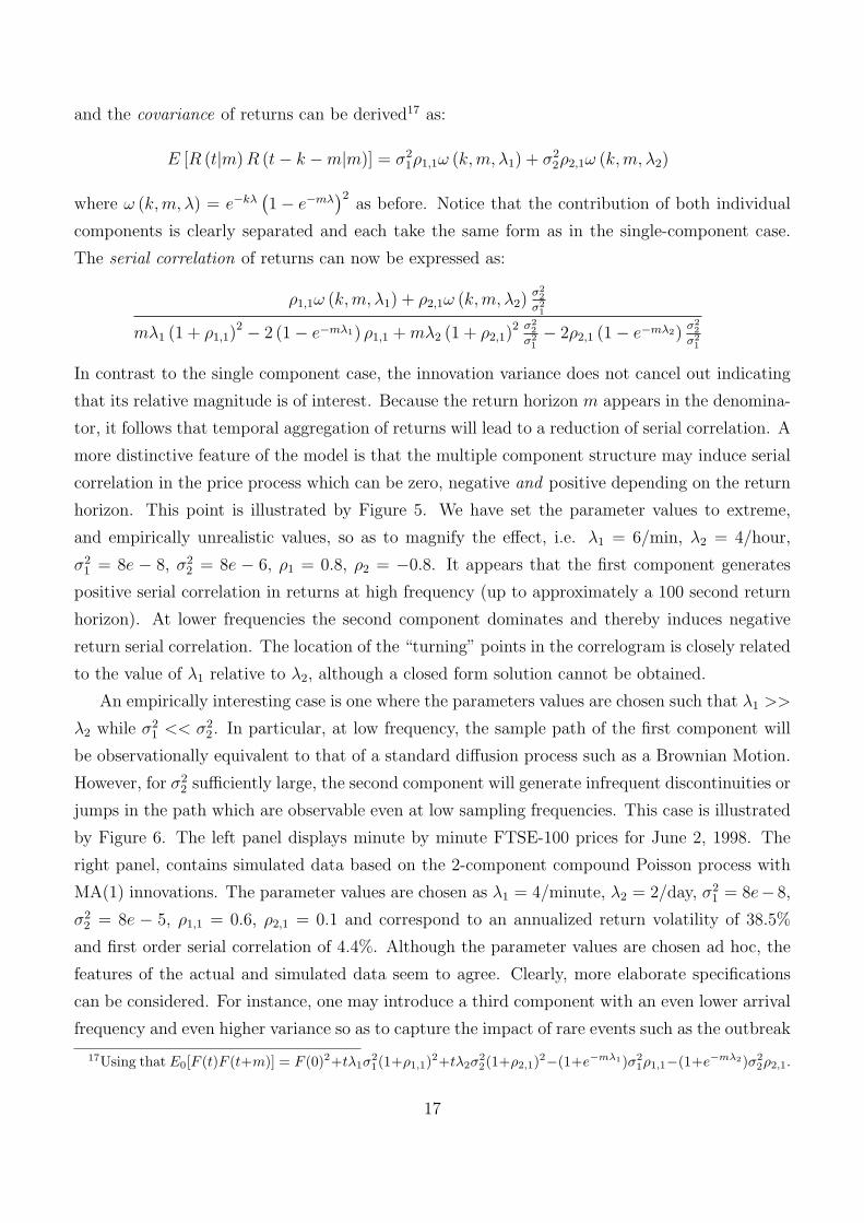
and the covariance of returns can be derived17 as:

E [R (t|m) R (t− k −m|m)] = σ21ρ1,1ω (k, m, λ1) + σ2

2ρ2,1ω (k, m, λ2)

where ω (k, m, λ) = e−kλ(1− e−mλ

)2as before. Notice that the contribution of both individual

components is clearly separated and each take the same form as in the single-component case.

The serial correlation of returns can now be expressed as:

ρ1,1ω (k, m, λ1) + ρ2,1ω (k,m, λ2)σ22

σ21

mλ1 (1 + ρ1,1)2 − 2 (1− e−mλ1) ρ1,1 + mλ2 (1 + ρ2,1)

2 σ22

σ21− 2ρ2,1 (1− e−mλ2)

σ22

σ21

In contrast to the single component case, the innovation variance does not cancel out indicating

that its relative magnitude is of interest. Because the return horizon m appears in the denomina-

tor, it follows that temporal aggregation of returns will lead to a reduction of serial correlation. A

more distinctive feature of the model is that the multiple component structure may induce serial

correlation in the price process which can be zero, negative and positive depending on the return

horizon. This point is illustrated by Figure 5. We have set the parameter values to extreme,

and empirically unrealistic values, so as to magnify the effect, i.e. λ1 = 6/min, λ2 = 4/hour,

σ21 = 8e − 8, σ2

2 = 8e − 6, ρ1 = 0.8, ρ2 = −0.8. It appears that the first component generates

positive serial correlation in returns at high frequency (up to approximately a 100 second return

horizon). At lower frequencies the second component dominates and thereby induces negative

return serial correlation. The location of the “turning” points in the correlogram is closely related

to the value of λ1 relative to λ2, although a closed form solution cannot be obtained.

An empirically interesting case is one where the parameters values are chosen such that λ1 >>

λ2 while σ21 << σ2

2. In particular, at low frequency, the sample path of the first component will

be observationally equivalent to that of a standard diffusion process such as a Brownian Motion.

However, for σ22 sufficiently large, the second component will generate infrequent discontinuities or

jumps in the path which are observable even at low sampling frequencies. This case is illustrated

by Figure 6. The left panel displays minute by minute FTSE-100 prices for June 2, 1998. The

right panel, contains simulated data based on the 2-component compound Poisson process with

MA(1) innovations. The parameter values are chosen as λ1 = 4/minute, λ2 = 2/day, σ21 = 8e− 8,

σ22 = 8e − 5, ρ1,1 = 0.6, ρ2,1 = 0.1 and correspond to an annualized return volatility of 38.5%

and first order serial correlation of 4.4%. Although the parameter values are chosen ad hoc, the

features of the actual and simulated data seem to agree. Clearly, more elaborate specifications

can be considered. For instance, one may introduce a third component with an even lower arrival

frequency and even higher variance so as to capture the impact of rare events such as the outbreak

17Using that E0[F (t)F (t+m)] = F (0)2+tλ1σ21(1+ρ1,1)2+tλ2σ

22(1+ρ2,1)2−(1+e−mλ1)σ2

1ρ1,1−(1+e−mλ2)σ22ρ2,1.

17

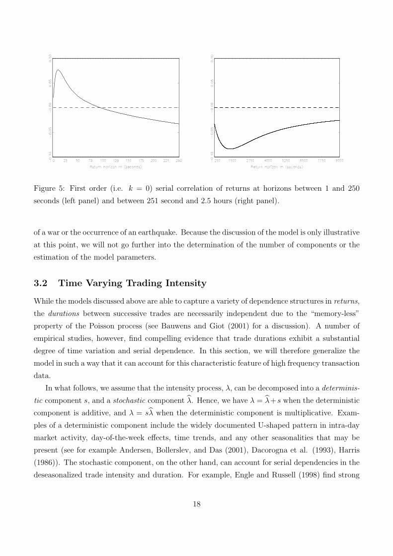
Figure 5: First order (i.e. k = 0) serial correlation of returns at horizons between 1 and 250

seconds (left panel) and between 251 second and 2.5 hours (right panel).

of a war or the occurrence of an earthquake. Because the discussion of the model is only illustrative

at this point, we will not go further into the determination of the number of components or the

estimation of the model parameters.

3.2 Time Varying Trading Intensity

While the models discussed above are able to capture a variety of dependence structures in returns,

the durations between successive trades are necessarily independent due to the “memory-less”

property of the Poisson process (see Bauwens and Giot (2001) for a discussion). A number of

empirical studies, however, find compelling evidence that trade durations exhibit a substantial

degree of time variation and serial dependence. In this section, we will therefore generalize the

model in such a way that it can account for this characteristic feature of high frequency transaction

data.

In what follows, we assume that the intensity process, λ, can be decomposed into a determinis-

tic component s, and a stochastic component λ. Hence, we have λ = λ+s when the deterministic

component is additive, and λ = sλ when the deterministic component is multiplicative. Exam-

ples of a deterministic component include the widely documented U-shaped pattern in intra-day

market activity, day-of-the-week effects, time trends, and any other seasonalities that may be

present (see for example Andersen, Bollerslev, and Das (2001), Dacorogna et al. (1993), Harris

(1986)). The stochastic component, on the other hand, can account for serial dependencies in the

deseasonalized trade intensity and duration. For example, Engle and Russell (1998) find strong

18

Figure 6: Minute by minute FTSE-100 index data (left panel) for June 2, 1998. Simulated

minute by minute data (right panel) using the 2-Component Compound Poisson process with

MA(1) innovations.

evidence of autoregressive serial dependence in deseasonalized intra-day trade durations which

motivates them to specify the Autoregressive Conditional Duration (ACD) model. Moreover, the

extensive evidence of ARCH effects in low frequency (say daily / weekly) return data indicates

that time variation in market activity is not only limited to intra-day frequencies, but extents

forcefully to lower frequencies. At this level, the stochastic component typically dominates the

deterministic one and, as a result, the time variation induced in low frequency return variance is

predominantly stochastic. In this section we will discuss specifications for both components of the

intensity process through which we seek to capture the following important stylized characteristics

of return data both at low and high frequency:

(i) seasonality in trade durations and market activity

(ii) serial dependence in deseasonalized trade duration

(iii) persistence in return variance at low sampling frequencies

We refer to property (ii) as “ACD”-effects and to property (iii) as “ARCH”-effects, thereby

alluding to the seminal work of Engle and Russell (1998), and Engle (1982) and Bollerslev (1986)

respectively. Because the aim is to capture all of the above effects through the specification of the

intensity process exclusively, a brief discussion of the relation between trading intensity, return

variance, and trade duration is in order. Recall that for the standard compound Poisson process

with unit innovation variance and (trade) intensity λ, the expected return variance over a unit

time interval equals λ while the expected trade duration is equal to 1/λ . Trading intensity is

19

thus proportional to return variance and inversely proportional to trade durations. However, these

relations may break down when we generalize the compound Poisson process. For example, when

a bid/ask spread “contaminates” the data, we have shown that the return variance is equal to λ

plus a non-linear correction term involving the spread. What’s more, when the trading intensity

is a (non-degenerate) deterministic function of time, the return variance equals∫

λ (u) du even

though the expected trade duration is not equal to 1/∫

λ (u) du. These cases are examples where

the proportionality between trading intensity, return variance, and inverse of trade duration, is

lost. However, it seems reasonable to expect that in many cases the proportionality will hold

approximately. Clearly, the extent to which this is true depends on the model specification and

also on the sampling frequency of the data (as we have shown that market microstructure effects

vanish under temporal aggregation).

Corollary 3.3 (to Theorem 3.1) For the price process defined by expression (7), with a non-

constant intensity process, λ (·), and M (t) >> q, the joint characteristic function of F (t) and

F (t + m), conditional on initial values, is accurately approximated by:

φ∗F (ξ1, ξ2, t,m) = E0

[eiξ1F (t)+iξ2F (t+m)

]= a(ξ)φ∗S (ξ1, ξ2, t,m) (11)

where φ∗S (ξ1, ξ2, t,m) equals:

eξ2σ2

νρ(q,q)

q−1∑

h=0

eiξ2hρµν− 12hσ2

νξ22ρ2

(e−ξ1ξ2σ2

νρ(q,h) − e−ξ1ξ2σ2νρ(q,q)

)E0

{b(ξ, 0, t

) (λ∗ (t,m))h

h!eλ∗(t,m)

}

+e(ξ2−ξ1ξ2)σ2

νρ(q,q)E0

{b(ξ, 0, t

)b (ξ2, t, m)

}

λ∗ (t, τ) ≡ ∫ t+τ

tλ (u) du, b (ξ, t, τ) = exp

[(eiξρµν− 1

2ξ2σ2

νρ2 − 1)

λ∗ (t, τ)], and ξ, ρ, a(ξ), ρ (q, p) are

as defined in Theorem 3.1.

For t →∞, the above expression of the characteristic function is exact.

Proof See Appendix C.

Allowing for time variation in the intensity process, leads to a modified characteristic function

of the price process as can be seen by comparing expression (11) in Corollary 3.3 to expression (

8) in Theorem 3.1. If time variation in the intensity process is entirely deterministic, or known at

t = 0, the expectation operator vanishes in the expression for φ∗S (ξ1, ξ2, t, m) and moments can be

derived in the usual fashion. This holds true irrespective of the, potentially complex, functional

form for λ (·). However, when time variation in the intensity process is (partly) stochastic, i.e.

unknown at t = 0, the expectations operator remains because the integrated intensity process is

now a random variable. Moments cannot be derived without explicit specification of the dynamics

of the intensity process, and even then, closed form solutions will not be available in many cases.

20

Deterministic Intensity Process. We will now briefly illustrate the usefulness of allowing for

deterministic variation in the intensity process. As mentioned above, one of the most prominent

features of high frequency data in financial markets is the U-shaped pattern in intra-day mar-

ket activity and return volatility. In particular, it is widely documented that market activity is

substantially higher around the open and close of the market than around lunch time. Another

important characteristic is that the overnight return typically accounts for a non-negligible frac-

tion of the overall daily return variance. While trading in many securities is halted overnight,

information flow is not. This in turn, leads to an accumulation of information which can only be

incorporated into the price at the next open of the market. The overnight return may therefore

reflect a disproportionately large amount of information relative to the subsequent intra-day re-

turns. A highly stylized specification of the intensity process, that is consistent with the above

observations, is the following:

λ (t) = a + b cos (2πt) + cI{t−[t]<∆} (12)

where a > b, c > 0, 0 < ∆ << 1, [t] denotes the integer part of t, and I is an indicator function

which equals 1 whenever t − [t] is less than ∆ and zero otherwise. Using the single component

compound Poisson process with MA(1) innovations and an intensity process as specified above, we

simulate 5 years of high frequency transaction prices using the following ad hoc parameter values;

a = 4/ minute, b = 2.25, c = 120/minute, ∆ = 2/480, ρ = 0.3, and σ2ν = 7e − 8. Based on 8

hours of trading per day, these parameters imply an average of 2160 trades per day, an annualized

daily return volatility of 25.4%, and a more than 25 fold increase in market activity (relative to

the daily average) during the first two minutes following the market open. The overnight return

aside, trading intensity at open and close (mid-day) is 50% higher (lower) than the daily average.

The left-hand panel of Figure 7 plots the correlogram of minute by minute absolute returns

on the FTSE-100 over the period 1990-2000. The displacement is up to 2400 lags, or equivalently,

five trading days. The U-shaped pattern in market activity and the impact of the overnight

return is apparent. Moreover, the magnitude of both effects underline the importance of allowing

for a deterministic pattern in the intensity process. The right-hand panel of Figure 7 plots the

correlogram for the simulated data sampled at minute intervals. The strong agreement among the

correlograms of the actual and simulated data demonstrates that the naive and overly simplistic

specification of the intensity process does capture important patterns in high frequency return

data at least to some extent. However, a more detailed inspection of the graphs points to some

important differences. For example, the correlogram for the FTSE-100 data indicates a peak in

market activity during the afternoon trading session that is, most likely, associated with the open

of the US markets. A more subtle difference in the correlogram for the actual data is that the

correlations are strictly positive at any displacement and that there appears to be a slow decline in

21

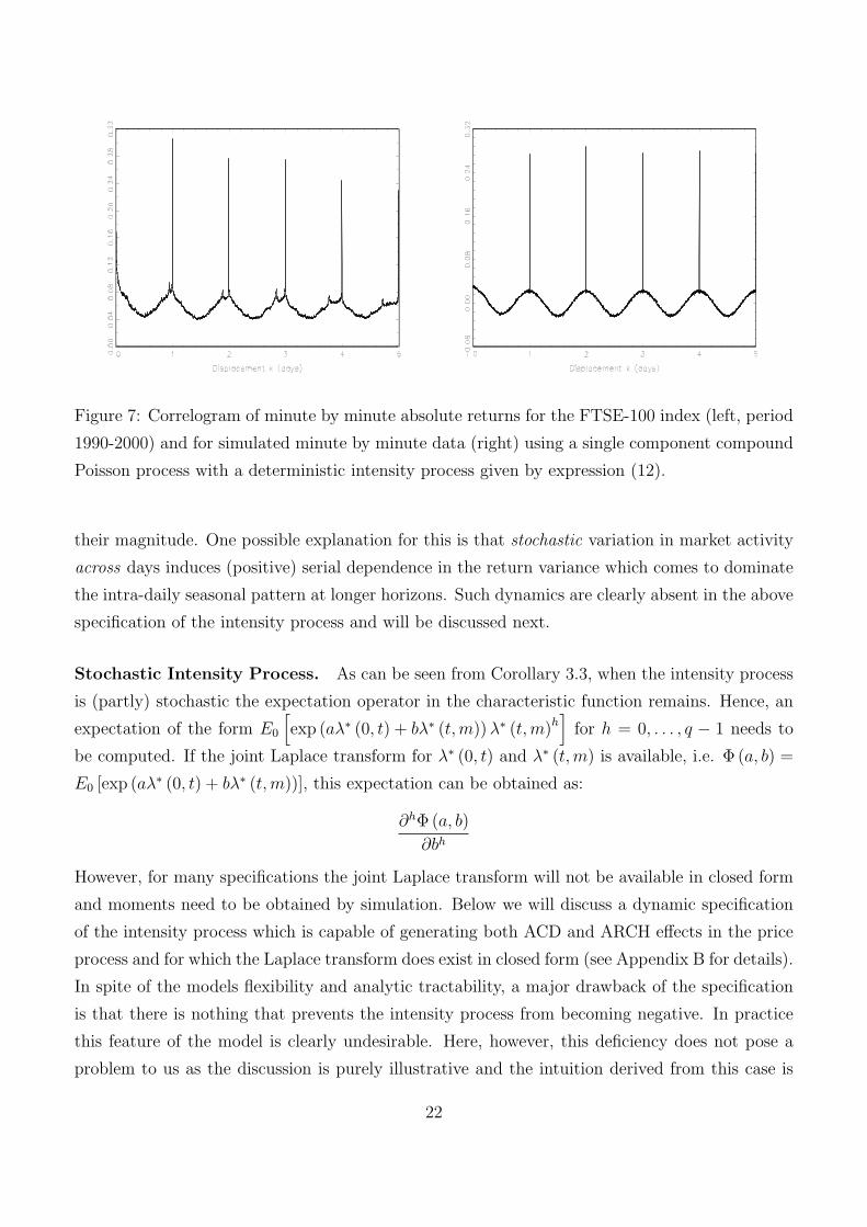
Figure 7: Correlogram of minute by minute absolute returns for the FTSE-100 index (left, period

1990-2000) and for simulated minute by minute data (right) using a single component compound

Poisson process with a deterministic intensity process given by expression (12).

their magnitude. One possible explanation for this is that stochastic variation in market activity

across days induces (positive) serial dependence in the return variance which comes to dominate

the intra-daily seasonal pattern at longer horizons. Such dynamics are clearly absent in the above

specification of the intensity process and will be discussed next.

Stochastic Intensity Process. As can be seen from Corollary 3.3, when the intensity process

is (partly) stochastic the expectation operator in the characteristic function remains. Hence, an

expectation of the form E0

[exp (aλ∗ (0, t) + bλ∗ (t,m)) λ∗ (t,m)h

]for h = 0, . . . , q − 1 needs to

be computed. If the joint Laplace transform for λ∗ (0, t) and λ∗ (t,m) is available, i.e. Φ (a, b) =

E0 [exp (aλ∗ (0, t) + bλ∗ (t,m))], this expectation can be obtained as:

∂hΦ (a, b)

∂bh

However, for many specifications the joint Laplace transform will not be available in closed form

and moments need to be obtained by simulation. Below we will discuss a dynamic specification

of the intensity process which is capable of generating both ACD and ARCH effects in the price

process and for which the Laplace transform does exist in closed form (see Appendix B for details).

In spite of the models flexibility and analytic tractability, a major drawback of the specification

is that there is nothing that prevents the intensity process from becoming negative. In practice

this feature of the model is clearly undesirable. Here, however, this deficiency does not pose a

problem to us as the discussion is purely illustrative and the intuition derived from this case is

22

likely to remain in tact for alternative specifications.

ACD and ARCH effects are known to unveil themselves at different frequencies and we there-

fore decompose the stochastic intensity process into a high frequency and a low frequency com-

ponent. In particular, ARCH effects are modelled through the low frequency component while

ACD effects are modelled through the high frequency component. Market microstructure con-

siderations are clearly of less importance for the low frequency component as they are for the

high frequency component. It therefore seems reasonable to rely on proportionality between

(integrated) intensity and (integrated) return variance when modelling the ARCH effects. For

this case, the dependence structure of the intensity process will (closely) corresponds to that of

the variance process and an appropriate specification for the low frequency component, α, is as

follows:

dα (t) = −ϕ (α (t)− µ) dt + σαdWα (t) , (13)

where ϕ ≥ 0, σα > 0, and Wα (t) is a standard Brownian motion. The above process is known

as the Ornstein-Uhlenbeck (OU) process and has the interesting property that it can be viewed

as the continuous-time analogue of the Gaussian first order regression. One way to see this is to

discretize the time scale as ti = i∆ where i = 1, . . . , T/∆ so that ∆ can be interpreted as the

frequency at which the continuous time process is sampled while T∆ represents the total number

of periods. The solution to the SDE in expression (13) can now be written as

α (ti) = µ(1− e−ϕ∆

)+ e−ϕ∆α (ti−1) + εti

where εti ∼ i.i.d. N(0, 1−e−2ϕ∆

2ϕσ2

α

). The discretized sample path of α thus follows an autoregres-

sive process of order one with autoregressive parameter equal to e−ϕ∆. Its persistence therefore

depends both on the parameter ϕ and the sampling frequency ∆. In particular, for fixed parame-

ters ϕ and σα, the persistence of the process increases with an increase of the sampling frequency

∆, i.e. smaller ∆ (see Boswijk (2002, Chapter 6) for more details). Because ARCH effects are

a low frequency phenomenon, we set ϕ and σα sufficiently small causing α to appear roughly

constant at high frequency. However, at lower frequencies, the mean reversion will become more

apparent, leading to an autoregressive dependence structure in return variance - ARCH effects.

The modelling of ACD-effects is unfortunately more complicated. At high frequency, market

microstructure effects and time variation in the intensity process can distort the proportionality

between trade intensity and trade duration. In addition, we need to address the question what

dependence structure should be imposed on the intensity process in order to generate ACD

effects, i.e. autoregressive dependence in the duration process. Even in idealized situations, there

is no clear answer to this question and we will proceed under the debatable assumption that ACD

effects can be captured by means of an autoregressive component in the (deseasonalized) intensity

23

process. With this in mind, we specify the high frequency component as follows:

dλ (t) = −κ(λ (t)− α (t)

)dt + σλdWλ (t) (14)

where κ ≥ 0, κ 6= ϕ, σλ > 0, and Wλ is a standard Brownian motion independent of Wα. The

process given by expression (14) is a generalization of the standard Gaussian OU process. It has

the property that λ mean-reverts towards the low frequency component, α, which itself varies

stochastically through time. In the current context, the difference between λ and α constitutes

the high frequency component of the intensity process. Quick mean reversion of λ towards the

stochastic long run mean, α, can be expected to generate mean reversion in the duration process

at high frequency, thereby leading to ACD effects. Hence, both ARCH and ACD effects can

be generated when ϕ << κ and σα << σλ and σ2α/ϕ >> σ2

λ/κ. At high sampling frequencies,

the process for λ will quickly “oscillate” around the stochastic long run mean α, which itself is

roughly constant due to its extreme persistence and small innovation variance relative to λ. The

stochastic time variation of the intensity process over short time intervals will therefore be mainly

driven by the OU process for λ whose mean reversion will lead to ACD effects. On the other hand,

at low(er) sampling frequencies, the stochastic variation in the average (or integrated) intensity

process arising from the OU process for λ will be minimal due to its quick mean reversion, and

at some stage the stochasticity of the long run mean component will come to dominate. Slow

mean reversion in α translates directly into slow mean reversion of trade intensity which, in turn,

leads to ARCH effects. Another way to see this is by considering the intensity variance at low

frequency which can be shown to equalσ2

λ

2κ+ κσ2

α

2ϕ(ϕ+κ)which is approximately equal to

σ2λ

2κ+ σ2

α

2ϕfor

k >> ϕ. Because, by assumption, the parameters are chosen such that σ2α/ϕ >> σ2

λ/κ, it is clear

that the stochastic long run mean dominates at low frequency. One can thus think of the OU

process for λ as driving time variation in the intensity process at high sampling frequencies, while

α has a “level-shifting” effect in the sense that it slowly moves the level at which λ operates.

In order to further illustrate this property of the model, we fix some ad hoc parameter values

that satisfy the above criteria, i.e. κ = 5, σλ = 0.25, ϕ = 0.0001, σα =√

0.001, and µ = 5. Next,

we simulate 2× 252 periods of the intensity process with 480 discretization steps per period. The

left panel of Figure 8 graphs a time series of intensity process λ over the first two periods of the

simulated sample. The superimposed dashed line represents the corresponding long run mean

component. It is clear that most of the variation in the intensity process at high frequency comes

from the OU dynamics of λ. The right panel of Figure 8 plots the period by period average (or

integrated) intensity process which corresponds very closely to the low frequency component (not

displayed). At this frequency, α drives the overall variation in the intensity process, while the

OU component for λ contributes little.

In summary, stochastic variation in the high and low frequency component of the intensity

24

Figure 8: Simulated intensity process (without deterministic component) based on the “double

OU” process as defined by expressions (13) and (14). The left panel plots the intensity process

at high frequency (solid line) for 2 periods together with its associated long run mean component

(dashed line). The right panel plots the average intensity process at lower frequency for the full

simulated sample of 504 periods.

process can lead to ACD and ARCH effects respectively. For the specification discussed above,

closed form solutions for the intensity process are available (see Appendix B for details). Because

the integrated intensity process turns out to be conditionally normal, a closed form expression

for the characteristic function in Corollary 3.3 is available. As mentioned above, a major flaw of

the model is that there is nothing that prevents the intensity process from becoming negative.

In the context of volatility modelling, Gupta and Subrahmanyam (2002), Stein and Stein (1991)

have used a similar specification and justified this on the basis that for a wide range of relevant

parameter values, the probability of actually reaching a negative value is so small as to be of

no significant consequence. Also, at this point the discussion of the model is purely illustrative

and the intuition derived from this case is likely to remain in tact for alternative specifications.

Nevertheless, in practice it may clearly make sense to sacrifice analytic tractability in return for a

more appropriate specification which ensures positivity of the intensity process. One approach is

to specify the model is terms of logarithmic intensity or incorporate a state-dependent innovation

variance as is done in the Feller or CIR process. Other models of potential interest are some of

the non-Gaussian OU processes discussed by Barndorff-Nielsen and Shephard (2001a).

25

4 Realized Variance and Return Dependence

In the context of the models analyzed above, we now study the impact of - market microstructure

induced - serial correlation in returns on the properties of the realized variance (RV) measure.

Importantly, we show that serial correlation renders the RV a biased estimator of the conditional

return variance. We derive closed form expressions for the bias term as a function of the sampling

frequency and the model parameters and show that the magnitude of the bias decays under

temporal aggregation of returns at a rate that is inversely proportional to the sampling frequency.

We also discuss the optimality of alternative sampling schemes.

In an influential series of papers Andersen, Bollerslev, Diebold, and Labys (2001, 2002, ABDL

hereafter) have shown that when the logarithmic price process follows a semi-martingale (i.e. a

process which can be decomposed into a finite variation component and a martingale component),

its associated quadratic variation (QV) process is a critical determinant of the conditional return

variance. Importantly, the QV process can - by definition - be approximated as the sum of squared

returns sampled at high frequency. It is this approximation of the QV process that is commonly

referred to as realized variance or volatility. In full generality, the relation between the conditional

return variance and the RV measure is not clear-cut. However, under certain (possibly restrictive)

assumptions on the finite variation component of the semimartingale, ABDL show that realized

variance is an efficient and unbiased estimator of the conditional return variance. ABDL also

argue that a violation of the assumptions ensuring unbiasedness is likely to have a trivial impact

on the properties of the RV measure, thereby establishing it as an unbiased, efficient, and robust

estimator of the conditional return variance. In the notation established above, ABDL exploit

the following equality:

E

N/m∑j=1

R (t + jm|m)2 |Ft

= E

[R (t + N |N)2 |Ft

]. (15)

where R denotes excess returns, m denotes the sampling frequency, whereas N denotes the length

of the period over which RV is calculated. It is clear from expression (15) that the unbiasedness of

the RV measure crucially relies on the martingale property of logarithmic (risk adjusted) prices,

or equivalently, the absence of serial correlation in excess returns. Nevertheless, a number of

recent studies have implemented the RV measure without much concern for possible violations

of the martingale assumption underlying the unbiasedness of this measure. It therefore seems

appropriate to study the dependence structure of high frequency returns and its associated impact

on the properties of the RV measure18. Although this is largely an empirical matter, and results

can be expected to vary across securities and time, the models discussed in this paper seem to

18See Andreou and Ghysels (2001), Bai, Russell, and Tiao (2001), and Oomen (2002) for related work.

26

capture a number of salient features of high frequency returns particularly well and are therefore

well suited to assess the properties of RV in a realistic, yet theoretical, setting.

4.1 The “Covariance Bias Term”

We investigate the properties of the RV measure for the single component compound Poisson

process with MA(1) innovations. Because the results for the “bid/ask model” take the same

form, we do not discuss this model separately. In the discussion below we distinguish between the

case where trade intensity is constant and the case where it is time varying. To simplify notation

we also set µ2ν = 0.

Constant Trade Intensity. Due to the stationarity of the return process, the conditional and

unconditional return variance coincide and can be expressed as

E[R(t + N |N)2

]= Nλσ2

ν (1 + ρ)2 − 2σ2νρ

(1− e−Nλ

) N large≈ Nλσ2ν (1 + ρ)2 (16)

On the other hand, the expectation of the RV measure is equal to19:

E

N/m∑j=1

R (t + jm|m)2

= Nλσ2

ν (1 + ρ)2

︸ ︷︷ ︸Return Variance

− 2(1− e−mλ

) Nρσ2ν

m︸ ︷︷ ︸Covariance Bias Term

(17)

In practice, N is typically large (e.g. a day or week) and the approximation error in expression

(16) can therefore safely be ignored. In contrast, m is typically small (e.g. minute or hour) and

the second term on the right hand side in expression (17) may therefore be substantial. This

illustrates a crucial point: when high frequency (intra-period) returns are used to construct the

19Using that∑N/m

j=1 (1− e−mλ) = (1− e−mλ)N/m.

27

RV measure, i.e. m < N , serial correlation of

returns induces a bias that is characterized by

the second term on the right hand side of ex-

pression (17). This bias can be either positive or

negative depending on the sign of ρ. Moreover,

the magnitude of the bias term decays at rate

m−1 under temporal aggregation while it tends

to −2Nλσ2νρ for m → 0. It is emphasized that

this result does not rely on the approximation

in expression (16) and will hold true as long as

intra-period return are used to construct the RV

measure, i.e. N > m. Clearly, the magnitude of

the bias will depend on specific parameter valuesFigure 9: Covariance Bias Term

and the sampling frequency.

This is illustrated in Figure 9. For20 ρ = 0.3 and ρ = −0.3, we plot the return variance

(standardized by N) plus the bias component for return horizons up to 10 minutes. The parameter

σ2ν is adjusted so as to maintain an annualized return variance of 25%, i.e. for ρ = 0.30 (ρ = −0.30)

we have σ2ν = 1.529e− 7 (σ2

ν = 5.272e− 7). It turns out that for these parameter values the bias

term is substantial, i.e. around 20% (12%) of the return variance when returns are negatively

(positively) correlated and sampled at the 1 minute frequency. The magnitude of this bias can

go up to 50% (20%) when sampled at even higher frequencies! These analytical results are in line

with a recent study by Oomen (2002) which finds that for the FTSE-100 index over the period

1990-2000 (i) high frequency returns feature substantial serial dependence (for minute by minute

data, the serial correlation is positive and significant up to high orders), (ii) the covariance bias

term is around 40% for minute by minute returns and (iii) the magnitude of this bias term decays

hyperbolically under temporal aggregation.

Time-Varying Trade Intensity For simplicity we focus on the case where the time variation

in the trading intensity is a deterministic function of time only. Although more general results can

be derived within the OU framework outlined above, the notation is complex and the stochastic

case does not add much additional insight for the discussion below. In the deterministic setting,

20Remember that the MA structure is imposed on returns in transaction time. For the bond futures data

analyzed in Section 2 we found a first order serial correlation of about −0.45. The chosen parameter values in the

simulation are therefore reasonable from an empirical point of view.

28

it directly follows from Corollary 3.3 that

E[RF (t + N |N)2] = σ2

ν (1 + ρ)2 λ∗ (t, N)− 2ρσ2ν

(1− e−λ∗(t,N)

) N large≈ σ2ν (1 + ρ)2 λ∗ (t, N)

On the other hand, the conditional expectation of RV is:

Et

N/m∑j=1

R (t + jm|m)2

= σ2

ν (1 + ρ)2 λ∗ (t, N)︸ ︷︷ ︸ReturnVariance

− 2ρσ2ν

N/m−1∑j=0

(1− e−λ∗(t+jm,m)

)

︸ ︷︷ ︸Covariance Bias Term

(18)

Again, the bias term can be substantial depending on the sampling frequency and model param-

eters and similar results can be derived for this case as for the constant intensity case. A more

interesting feature of the bias characterization for non-constant trade intensity, is that it allows

us to analyze the performance of alternative sampling schemes to which we turn next.

4.2 Bias Reduction and Optimality of Sampling Schemes

As pointed out above, the presence of serial correlation in returns introduces a bias in the RV

measure which can be substantial for realistic model parameter values. Because the efficiency of

the RV measure crucially relies on the use of intra-period returns, one faces a trade off between the

sampling returns at a high frequency, thereby minimizing the measurement error, and sampling

returns at low frequency, thereby minimizing the bias term. This trade-off suggest the existence

of an “optimal” sampling frequency, that is the highest available frequency at which the bias

term is negligible. Alternatively, one could estimate the model parameters and correct for the

bias term based on the expression derived above. In practice it is not clear which of these two

approaches is preferable. While the bias correction method allows one to use all available data,

it is clearly model dependent. The gain in efficiency may therefore be offset by the impact of

model and parameter uncertainty. On the other hand, while specifying an “optimal” sampling

frequency is essentially non-parametric or model independent, valuable information may be lost

by the aggregation of returns.

A related issue that arises in this context is how to sample the data. Up to now we have only

considered returns that are sampled at equidistant time intervals, i.e. t+ jm for j = 1, . . . , N/m.

However, when transaction data is available it is also possible to consider alternative sampling

schemes. A particularly interesting one is where the price process is sampled at time points τj

for j = 1, . . . , N/m where τ0 = t, τN/m = t + N and

∫ τj+1

τj

λ(u)du =m

N

∫ τN/m

τ0

λ(u)du ≡ λm (19)

29

The above sampling scheme effectively “deforms” the calendar time scale by compressing it when

the arrival rate of trades is low and stretching it when the arrival rate of trades is high. In

this case, one can think of returns being equally spaced on a “transaction” or “business” time

scale as opposed to a calendar time scale. An attractive feature of this sampling scheme is that

the statistical properties of returns sampled on this deformed time scale coincide with those of

a homogenous compound Poisson process with intensity parameter equal to λm. Because the

construction in expression (19) ensures that both sampling schemes generate the same number

of intra-period returns (N/m), it is of interest to compare the bias term associated with each

scheme. As can be seen from expression (18), for the calendar time sampling, the bias term is

equal to:

2ρσ2ν

N/m−1∑j=0

(1− e−λ∗(t+jm,m)

)

On the other hand, for the “business time” sampling, the bias is simply:

2ρσ2ν

N/m−1∑j=0

(1− e−λm

)

Surprisingly, it turns out that the bias term associated with calendar time sampled returns is

strictly smaller than the bias term associated with “business time” sampled returns. In order to

show this it is sufficient to prove that

N/m−1∑j=0

e−λ∗(t+jm,m) >

N/m−1∑j=0

e−λm or equivalently R ≡ m

N

N/m−1∑j=0

eλm−λ∗(t+jm,m) > 1

By the definition of λm and the convexity of the exponential function, the above inequality must

hold as long as the intensity parameter is non-constant. Note that R measures the bias reduction

associated with calendar time sampling relative to transaction sampling. This gain increases with

an increase in the variability of λ(·). When the intensity parameter is constant, we have that

R = 1, and both sampling schemes are equivalent.

4.2.1 Bias versus Mean Squared Error

The approach outlined above, classifies competing sampling schemes solely based on the relative

magnitude of its associated bias. An alternative well known measure of performance21 is the

mean squared error (MSE) which trades off a reduction in the bias against the loss of efficiency.

While we have shown that calendar time sampling strictly dominates business time sampling

when we use a bias-based ranking, it may very well be that this result is reversed when we use an

21I am indebted to Jeff Russell for pointing this out to me.

30

MSE-based ranking which takes both bias and efficiency into account. Unfortunately, an analytic

treatment of an MSE-based ranking of competing sampling schemes is not feasible because we

do not have a closed form solution for the variance of the RV measure available. A small-scale

simulation experiment is therefore undertaken to gauge whether an MSE-based ranking will yield

qualitatively different results than the bias-based ranking.

We focus on the single component compound Poisson process with MA(1) innovations and

deterministic time variation of the intensity process, i.e. λ (t) = s (t). The specification we use for

s (t) is similar to expression (12) with the indicator function left out. The parameter values are the

same as discussed on page 21. Next, we simulate T = 1000 (disjoint) days of transaction prices.

Let Ft (u) denote the security price at time u during day t where u ⊂ [0, N ] and t = 1, . . . , T . In

addition, let Ft (τi) denote the security price associated with the ith transaction on day t. The

implementation of calendar time sampling is straightforward, i.e. for a given day t and a sampling

frequency m, we sample N/m returns as

Rct (j|m) = Ft (jm)− Ft ((j − 1) m)

for j = 1, . . . , N/m. The corresponding business time sampling scheme, in contrast, samples the

same amount of returns as follows:

Rbt (j|k) = Ft (τjk)− Ft

(τ(j−1)k

)

for j = 1, . . . , N/m and k = mnt/N where nt denotes the total number of transactions for day t.

Based on these returns series we construct the following statistics:

CBS (m) = Et

[R2

t

]− 1

T

T∑t=1

N/m∑j=1

Rct (j|m)2 ,

BBS (m) = Et

[R2

t

]− 1

T

T∑t=1

N/m∑j=1

Rbt (j|k)2 ,

and

CMSE (m) =1

T

T∑t=1

Et

[R2

t

]−N/m∑j=1

Rct (j|m)2

,

BMSE (m) =1

T

T∑t=1

Et

[R2

t

]−N/m∑j=1

Rbt (j|m)2

.

Figure 10 displays all of the above statistics for sampling frequencies (m) between 1 second and

5 minutes. A number of interesting patterns arise. As expected, based on the bias-ranking, the

31

Figure 10: Covariance Bias term (CBS and BBS, left panel) and Mean Squared Error (CMSE

and BMSE, right panel) for “Calendar” or “Physical” Clock (solid line) and “Business Clock”

(dashed line) sampling schemes.

calendar time scheme dominates. However, the difference in performance between both schemes

rapidly shrinks as the sampling frequency decreases. At sampling frequencies lower than 1 minute,

the difference is minimal which implies that the optimal sampling frequency will be the same for

both schemes. In contrast, when the MSE is used to rank the sampling schemes, it appears that

the business time sampling achieves the lowest overall MSE. Moreover, the sampling frequency

which minimizes the MSE is substantially higher than the sampling frequency which minimizes

the bias. Ignoring the efficiency loss associated with aggregation of returns, as is done for the

bias-based ranking, clearly leads one to choose a much lower sampling frequency than if the MSE

is taken as the relevant performance measure. Based on this simulation experiment we conclude

that business time sampling dominates calendar time sampling when the objective is to either

minimize the bias (in which case both schemes perform roughly equal) or minimize the MSE (in

which case business time sampling dominates).

5 Conclusion

This article studies several extensions of the compound Poisson process which are able to cap-

ture important static and dynamic characteristics of high frequency security prices. In contrast

to diffusion-based models, our framework is consistent with the finite variation property of high

frequency returns and does not impose the usual martingale restriction on asset prices. By com-

paring the properties of simulated data to actual high frequency data we illustrate the flexibility

32

of the model and its ability to capture important features of high frequency data including, (i)

skewness, excess kurtosis and return serial correlation which diminishes under temporal aggrega-

tion, (ii) deterministic variation in trading activity such as the U-shaped intra-day pattern, day of

the week effects, and the increased variance of the overnight return, and (iii) stochastic variation

in trading activity leading to serial dependence in trade durations at high frequency (ACD-effects)

and return volatility at low frequency (ARCH-effects). In addition, our models provide a use-

ful context in which to investigate “market-microstructure-induced” serial correlation of returns

at different sampling frequencies and its associated impact on the recently popularized realized

volatility or variance measure. In particular, we show that for realistic parameter values the

realized variance measure is a biased estimator of the integrated variance process and that the

choice of sampling frequency proves crucial in minimizing this bias. Finally, allowing for time

variation in the trade intensity process yields interesting insights into the properties of alternative,

time-deformation-based, sampling schemes.

33

References

Admati, A., and P. Pfeiderer, 1988, “A Theory of Intraday Patterns: Volume and Price Variabil-

ity,” Review of Financial Studies, 1 (1), 3–40.

Andersen, P. K., Ø. Borgan, R. Gill, and N. Keiding, 1993, Statistical Models Based on Counting

Processes. Springer-Verlag, New York.

Andersen, T. G., 1996, “Return Volatility and Trading Volume: An Information Flow Interpre-

tation of Stochastic Volatility,” Journal of Finance, 51 (1), 169–204.

Andersen, T. G., L. Benzoni, and J. Lund, 2002, “An Empirical Investigation of Continuous-Time

Equity Return Models,” Journal of Finance, 57(3), 1239–1284.

Andersen, T. G., T. Bollerslev, and A. Das, 2001, “Variance-Ratio Statistics and High Frequency

Data: Testing for Changes in Intraday Volatility Patterns,” Journal of Finance, 56 (1), 305–

327.

Andersen, T. G., T. Bollerslev, F. X. Diebold, and P. Labys, 2001, “The Distribution of Realized

Exchange Rate Volatility,” Journal of the American Statistical Association, 96, 42–55.

, 2002, “Modelling and Forecasting Realized Volatility,” forthcoming Econometrica.

Andreou, E., and E. Ghysels, 2001, “When Does Microstructure Noise Affect the Estimation of

Asset Pricing Models?,” Manuscript University of Manchester and North Carolina.

Ane, T., and H. Geman, 2000, “Order Flow, Transaction Clock, and Normality of Asset Returns,”

Journal of Finance, 55(5), 2259–2284.

Bai, X., J. R. Russell, and G. C. Tiao, 2001, “Beyond Merton’s Utopia (I): Effects of Non-

Normality and Dependence on the Precision of Variance Estimates using High Frequency Data,”

Manuscript University of Chicago.

Bakshi, G., C. Cao, and Z. Chen, 1997, “Empirical Performance of Alternative Option Pricing

Model,” Journal of Finance, 52(5), 2003–2049.

Bakshi, G., and D. Madan, 2000, “Spanning and Derivative-Security Valuation,” Journal of

Financial Economics, 55(2), 205–238.

Barndorff-Nielsen, O. E., and N. Shephard, 2001a, “Non-Gaussian Ornstein-Uhlenbeck-Based

Model and Some of Their Uses in Financial Economics,” Journal of the Royal Statistical Society,

Series B, 63 (2), 167–241.

34

, 2001b, “Realized Power Variation and Stochastic Volatility Models,” Manuscript Oxford

University.

Bates, D. S., 1996, “Jumps and Stochastic Volatility: Exchange Rate Processes Implicit in

Deutsche Mark Options,” Review of Financial Studies, 9(1), 69–107.

, 2000, “Post-87 Crash Fears in the S&P 500 Futures Option Market,” Journal of Econo-

metrics, 94(1/2), 181–238.

Bauwens, L., and P. Giot, 2001, Econometric Modelling of Stock Market Intraday Activity. Kluwer

Academic Publishers, Boston.

Bollerslev, T., 1986, “Generalized autoregressive conditional heteroskedasticity,” Journal of

Econometrics, 51, 307–327.

Bollerslev, T., and H. Zhou, 2002, “Estimating Stochastic Volatility Diffusion using Conditional

Moments of Integrated Volatility,” Journal of Econometrics, 109, 33–65.

Boswijk, H. P., 2002, Asymptotic Theory for Integrated Processes. manuscript in preparation for

Oxford University Press, Oxford.

Campbell, J. Y., A. W. Lo, and A. C. MacKinlay, 1997, The Econometrics of Financial Markets.

Princeton University Press, Princeton, NJ.

Carr, P., H. Geman, D. B. Madan, and M. Yor, 2002, “Stochastic Volatility for Levy Processes,”

fortcoming Mathematical Finance.

Carr, P., and L. Wu, 2002, “Time-Changed Levy Processes and Option Pricing,” forthcoming

Journal of Financial Economics.

Chan, W. H., and J. M. Maheu, 2002, “Conditional Jump Dynamics in Stock Market Returns,”

Journal of Business and Economic Statistics, 20 (3), 377–389.

Clark, P. K., 1973, “A Subordinated Stochastic Process Model with Finite Variance for Specula-

tive Prices,” Econometrica, 41(1), 135–155.

Cox, J. C., and S. A. Ross, 1976, “The Valuation of Options for Alternative Stochastic Processes,”

Journal of Financial Economics, 3(1/2), 145–166.

Dacorogna, M. M., U. A. Muller, R. J. Nagler, R. B. Olsen, and O. V. Pictet, 1993, “A Geo-

graphical Model for the Daily and Weekly Seasonal Volatility in the Foreign Exchange Market,”

Journal of International Money and Finance, 12, 413–438.

35

Demsetz, H., 1968, “The Cost of Transacting,” Quarterly Journal of Economics, 82, 33–53.

Duffie, D., J. Pan, and K. J. Singleton, 2000, “Transform Analysis and Asset Pricing for Affine

Jump-Diffusions,” Econometrica, 68(6), 1343–1376.

Easley, D., N. Kiefer, and M. O’Hara, 1997, “One Day in the Life of a Very Common Stock,”

Review of Financial Studies, 10 (3), 805–835.

Easley, D., and M. O’Hara, 1992, “Time and the Process of Security Price Adjustment,” Journal

of Finance, 47 (2), 577–605.

Embrechts, P., C. Kluppelberg, and T. Mikosch, 1997, Modelling Extremal Events for Insurance

and Finance. Springer-Verlag, Berlin and Heidelberg.

Engle, R. F., 1982, “Autoregressive conditional heteroskedasticity with estimates of the variance

of U.K. inflation,” Econometrica, 50, 987–1008.

Engle, R. F., and J. R. Russell, 1998, “Autoregressive Conditional Duration: A New Model for

Irregularly Spaced Transaction Data,” Econometrica, 66(5), 1127–1162.

Eraker, B., 2001, “Do Stock Prices and Volatility Jump? Reconciling Evidence from Spot and

Option Prices,” Manuscript Duke University.

Feller, W., 1968, An Introduction to Probability Theory and Its Applications, vol. 1. Wiley, New

York, 3 edn.

Glosten, L., and P. R. Milgrom, 1985, “Bid, Ask and Transaction Prices in a Specialist Market

with Heterogeneously Informed Traders,” Journal of Financial Economics, 14, 71–100.

Gupta, A., and M. G. Subrahmanyam, 2002, “Pricing and Hedging Interest Rate Options: Evi-

dence from Cap-Floor Markets,” manuscript Leonard N. Stern School of Business, New York

University.

Harris, L., 1986, “A Transaction Data Study of Weekly and Intradaily Pattens in Stock Returns,”

Journal of Financial Economics, 16, 99–117.

Harrison, J. M., and D. M. Kreps, 1979, “Martingales and Arbitrage in Multiperiod Securities

Markets,” Journal of Economic Theory, 2(3), 381–408.

Heston, S. L., 1993, “A Closed Form Solution for Options with Stochastic Volatility with Appli-

cations to Bond and Currency Options,” Review of Financial Studies, 6, 327–344.

36

Ho, T., and H. Stoll, 1983, “The Dynamics of Dealer Markets under Competition,” Journal of

Finance, 38, 1053–1074.

Huang, R., and H. Stoll, 1997, “The Components of the Bid-Ask Spread: A General Approach,”

Review of Financial Studies, 10 (4), 995–1034.

Jiang, G. J., and J. L. Knight, 2002, “Estimation of Continuous-Time Processes Via the Empirical

Characteristic Function,” Journal of Business & Economic Statistics, 20 (2), 198–212.

Karatzas, I., and S. E. Shreve, 1991, Brownian Motion and Stochastic Calculus. Spinger-Verlag,

New York.

Karlin, S., and H. M. Taylor, 1981, A Second Course in Stochastic Processes. Academic Press,

New York.

, 1997, A First Course in Stochastic Processes. Academic Press, New York.

Kendall, M., 1958, The Advanced Theory of Statistics, vol. I. Hafner Publishing Co., New York.

Kyle, A. S., 1985, “Continuous Auctions and Insider Trading,” Econometrica, 53 (6), 1315–1335.

Lo, A. W., and A. C. MacKinlay, 1990, “An Econometric Analysis of Nonsynchronous-Trading,”

Journal of Econometrics, 45, 181–212.

Madan, D. B., and E. Seneta, 1984, “Compound Poisson Models for Economic Variable Move-

ments,” Sankhya Series B, 46, 174–187.

Madhavan, A. N., 2000, “Market Microstructure: A Survey,” Journal of Financial Markets, 3,

205–258.

Maheu, J. M., and T. H. McCurdy, 2002, “News Arrival, Jump Dynamics and Volatility Compo-

nents for Individual Stock Returns,” Manuscript University of Toronto.

Murmann, A., 2001, “Pricing Catastrophe Insurance Derivatives,” Manuscript Insurance and Risk

Management Department, The Wharton School.

O’Hara, M., 1995, Market Microstructure Theory. Blackwell Publishers Ltd, Oxford, UK.

Oomen, R. C., 2002, “Modeling Realized Variance when Returns are Serially Correlated,”

Manuscript European University Institute.

Pan, J., 2002, “The Jump-Risk Premia Implicit in Options: Evidence from an Integrated Time-

Series Study,” Journal of Financial Economics, 63, 3–50.

37

Press, S. J., 1967, “A Compound Events Model for Security Prices,” Journal of Business, 40(3),

317–335.

, 1968, “A Modified Compound Poisson Process with Normal Compounding,” Journal of

the American Statistical Association, 63, 607–613.

Rogers, L., and O. Zane, 1998, “Designing and Estimating Models of High-Frequency Data,”

Manuscript University of Bath.

Roll, R., 1984, “A Simple Implicit Measure of the Effective Bid-Ask Spread in an Efficient Mar-

ket,” Journal of Finance, 39(4), 1127–1139.

Rolski, T., H. Schmidli, V. Schmidt, and J. Teugels, 1999, Stochastic Processes for Insurance and

Finance. John Wiley & Sons, Chichester.

Rydberg, T. H., and N. Shephard, 2003, “Dynamics of Trade-by-Trade Price Movements: De-

composition and Models,” forthcoming Journal of Financial Econometrics.

Scott, L., 1997, “Pricing Stock Options in a Jump-Diffusion Model with Stochastic Volatility

and Interest Rates: Applications of Fourier Inversion Methods,” Mathematical Finance, 7(4),

413–426.

Stein, E., and J. Stein, 1991, “Stock price distributions with stochastic volatility: An analytic

approach,” Review of Financial Studies.

Stoll, H., 1978, “The Pricing of Security Dealer Services: An Empirical Study of NASDAQ

Stocks,” Journal of Finance, 33 (4), 1153–1172.

Wood, R., 2000, “Market Microstructure Research Databases: History and Projections,” Journal

of Business & Economic Statistics, 18(2), 140–145.

38

A The Characteristic Function

Following Feller (1968), let X denote a random variable with probability measure µ. The char-

acteristic function of X (or µ) is the function φ (ξ) defined for real ξ by:

φ (ξ) ≡ E[eiξX

]=

∫ ∞

−∞eiξxµ (dx) =

∫ ∞

−∞(cos (ξx) + i sin (ξx)) µ (dx) .

The characteristic function of aX + b equals eibξφ (aξ). When X is Gaussian with zero mean and

unit variance φ (ξ) = e−12ξ2

. Non-central moments (mn) and cumulants (κn) of order n can be

derived as:

mn = i−n ∂nφ (ξ)

∂ξn|ξ=0 and κn = i−n ∂n ln φ (ξ)

∂ξn|ξ=0

There exists a one-to-one relationship between moments and cumulants of any order. For the

first four orders they are as follows: κ1 = m1, κ2 = m2 − m21, κ3 = m3 − 3m1m2 + 2m3

1, and

κ4 = m4 − 3m22 − 4m1m3 + 12m2

1m2 − 6m41. See Kendall (1958) for more details. The joint

characteristic function of the set of random variables {Xj}kj=1 is given by:

φ (ξ1, . . . , ξk) ≡ E [exp (iξ1X1 + iξ2X2 + . . . + iξkXk)] ,

which generates joint moments as follows:

E [Xp1

1 Xp2

2 · · ·Xpk

k ] = i−p ∂pφ (ξ1, . . . , ξk)

∂ξp1

1 ∂ξp2

2 · · · ∂ξpk

k

|ξ=0,

where p =∑k

i=1 pi.

B The Intensity Process

The solution to the SDE in expression (14) directly follows from a general result on one-dimensional

linear SDE as discussed by Karatzas and Shreve (1991, Section 5.6C):

λ (t + τ) = e−κτ λ (t) + κ

∫ t+τ

t

e−κ(t+τ−u)α (u) du + σλ

∫ t+τ

t

e−κ(t+τ−u)dWλ (u) . (20)

for τ > 0. The OU specification for α allows us to further specialize expression (20) above:

λ (t + τ) = µ + e−κτ(λ (t)− µ

)+

κ (e−κτ − e−ϕτ )

ϕ− κ(α (t)− µ) (21)

+κσα

∫ t+τ

t

e−ϕ(t+τ−u) − e−κ(t+τ−u)

κ− ϕdWα (u) + σλ

∫ t+τ

t

e−κ(t+τ−u)dWλ (u)

using that∫ t+τ

t

f (h)

{∫ h

t

g (h, u) dW (u)

}dh =

∫ t+τ

t

{∫ t+τ

u

f (h) g (h, u) dh

}dW (u) (22)

where f (h) and g (h, u) are deterministic functions. Based on expression (21) above, it is straight-

forward to derive an expression for the integrated intensity process.

39

C Proofs

Proof of Theorem 2.1 Let the characteristic function of innovations to the mid-price be given

by

φε (η) = E0

[eiηε

]= eiηµI− 1

2η2σ2

I

where ε ∼ N (µI , σ2I ). Now derive the characteristic function of the mid-price process, i.e.

φF (η, t) = E0

[eiηF (t)

]. Define S (n) =

∑nj=1 εj and notice that

φF (η, t) =∞∑

n=0

(tλI)n e−tλI

n!E0

[eiη(F (0)+S(n))

]= eiηF (0)−tλI

∞∑n=0

(tλIe

iηµI− 12η2σ2

I

)n

n!

= eiηF (0)−tλI

∞∑n=0

[tλIφε (η)]n

n!= eiηF (0)+tλI(φε(η)−1)

using that S (n) ∼ N (nµI , nσ2I ) and

∑∞n=0

an

n!= ea. To derive the joint characteristic function of

F and G, i.e. φF,G (η, ξ, t) = E0

[eiηF (t)+iξG(t)

], use that:

φF,G (η, ξ, t + h)− φF,G (η, ξ, t) = E0

(eiηF (t)+iξG(t)Et

[eiηRF (t+h|h)+iξRG(t+h|h) − 1

]).

Consider the random variable eiηRF (t+h|h)+iξRG(t+h|h) and notice that, for h sufficiently small, the

memory-less property of the Poisson process implies:

Pr[eiηRF (t+h|h)+iξRG(t+h|h) = e−iξG(t)+iηεMI (t+h)

]= hλI ,

Pr[eiηRF (t+h|h)+iξRG(t+h|h) = eiξ(−δ−G(t))

]= hλS,

Pr[eiηRF (t+h|h)+iξRG(t+h|h) = eiξ(δ−G(t))

]= hλB,

Pr[eiηRF (t+h|h)+iξRG(t+h|h) = 1

]= 1− hλ,

where εMI(t+h) ∼ N (µI , σ2I ). Therefore

Et

[eiηRF (t+h|h)+iξRG(t+h|h) − 1

]= hλIe

−iξG(t)EteiηεMI (t+h) + hλBeiξ(δ−G(t)) + hλSeiξ(−δ−G(t)) − hλ

Multiplying with eiηF (t)+iξG(t) yields:

Et

[eiηF (t+h)+iξG(t+h) − eiηF (t)+iξG(t)

]=

[hλIEte

iηεMI (t+h) + hλBeiξδ + hλSe−iξδ]eiηF (t)−hλeiηF (t)+iξG(t)

Taking expectations of the above expression, dividing by h, and taking h to zero results in:

∂φF,G (η, ξ, t)

∂t= lim

h→0

φF,G (η, ξ, t + h)− φF,G (η, ξ, t)

h

=[λIφε (η) + λBeiξδ + λSe−iξδ

]φF (η, t)− λφF,G (η, ξ, t) , (23)

40

with the expressions for φε (η, t) and φF (η, t) given above. Solving the differential equation in

expression (23), subject to the boundary condition φF,G (η, ξ, 0) = eiηF (0)+iξG(0), yields the joint

characteristic function of F and G:

φF,G (η, ξ, t) = f (η, ξ)(φF (η, t)− eiηF (0)−tλ

)+ eiηF (0)+iξG(0)−tλ

where

f (η, ξ) =λIφε (η) + λBeiξδ + λSe−iξδ

λIφε (η) + λB + λS

This completes the proof of expression 6.

Now, based on the joint characteristic function of F and G, it is straightforward to derive that

for m > 0:

φ∗F,G (η1, η2, ξ1, ξ2, t, m) = E0

[eiη1F (t)+iη2F (t+m)+iξ1G(t)+iξ2G(t+m)

]

= E0

[eiη1F (t)+iξ1G(t)Ete

iη2F (t+m)+iξ2G(t+m)]

= E0

[eiη1F (t)+iξ1G(t)a (η2, ξ2)

(φF,t (η2,m)− eiη2F (t)−mλ

)]

+E0

[eiη1F (t)+iξ1G(t)eiη2F (t)+iξ2G(t)−mλ

]

= f (η2, ξ2) φF,G (η1 + η2, ξ1, t)(emλI(φε(η2)−1) − e−mλ

)

+e−mλφF,G (η1 + η2, ξ1 + ξ2, t)

which completes the proof of expression 5.

Proof of Theorem 3.1 Define the cumulative innovations S (n) =∑n

j=1 εj and notice that the

joint characteristic function of F (t) and F (t + m) can be written as

E0

[eiξ1F (t)+iξ2F (t+m)

]= a(ξ)φ∗S (ξ1, ξ2, t, m)

where φ∗S (ξ1, ξ2, t, m) ≡ E0

[eiξ1S(MI(t))+iξ2S(MI(t+m))

], ξ = ξ1 + ξ2 and a(ξ) = exp(iξF (0)). The

variance of S (n) equals:

Σq (n) = nσ2ν

q∑j=0

ρ2j + 2σ2

ν

min(q,n)∑

h=1

q∑

j=h

(n− h) ρjρj−h, (24)

which, for n ≥ q, simplifies to:

Σq (n) = nσ2νρ

2 − 2σ2νρ (q, q) ,

where ρ =∑q

j=0 ρj and

ρ (q, k) =

{ ∑min(q,k)h=1

∑qj=h hρjρj−h for q ≥ 1, k ≥ 1

0 otherwise

41

Note that S (n) ∼ N (nρµν , Σq (n)) and thus E[eiξS(n)

]= eiξnρµν− 1

2ξ2Σq(n). The covariance of

S (n) and S (n + h) equals:

Σq (n, h) = Σq (n) + σ2νρ (q, h) ,

and because S (n) and S (n + h) are jointly normal, their joint characteristic function can be

derived as:

E0

[eiξ1S(n)+iξ2S(n+h)

]= eiξnρµν+iξ2hρµν− 1

2 [ξ21Σq(n)+ξ2

2Σq(n+h)+2ξ1ξ2Σq(n,h)]

= eiξnρµν+iξ2hρµνe−12 [(ξ2

1+2ξ1ξ2)Σq(n)+ξ22Σq(n+h)+2ξ1ξ2σ2

νρ(q,h)]

Recall that

φ∗S (ξ1, ξ2, t, m) = E0

[ ∞∑

h=0

∞∑n=0

eiξ1S(n)+iξ2S(n+h) (mλ)h

h!emλ

(tλ)n

n!etλ

](25)

which, for t sufficiently large22, can be approximated accurately by:

eξ2σ2

νρ(q,q)

∞∑

h=0

eiξ2hρµν− 12 [hξ2

2σ2νρ2+2ξ1ξ2σ2

νρ(q,h)] (mλ)h

h!emλ

∞∑n=0

eiξnρµν− 12ξ2nσ2

νρ2 (tλ)n

n!etλ

= b(ξ, t

)eξ

2σ2

νρ(q,q)

∞∑

h=0

eiξ2hρµν− 12 [hξ2

2σ2νρ2+2ξ1ξ2σ2

νρ(q,h)] (mλ)h

h!emλ

where b (ξ, t) = exp[tλ

(eiξρµν− 1

2ξ2σ2

νρ2 − 1)]

. The summation over h can be rewritten as:

q−1∑

h=0

eiξ2hρµν− 12 [hσ2

νξ22ρ2+2ξ1ξ2σ2

νρ(q,h)] (mλ)h

h!emλ+ e−ξ1ξ2σ2

νρ(q,q)

∞∑

h=q

eiξ2hρµν− 12hξ2

2σ2νρ2 (mλ)h

h!emλ

where∞∑

h=q

eiξ2hρµν− 12hσ2

νξ22ρ2 (mλ)h

h!emλ= b (ξ2,m)−

q−1∑

h=0

eiξ2hρµν− 12hσ2

νξ22ρ2 (mλ)h

h!emλ

Collecting above expressions yields:

φ∗S (ξ1, ξ2, t, m) = b(ξ, t

)eξ

2σ2

νρ(q,q)

q−1∑

h=0

eiξ2hρµν− 12hσ2

νξ22ρ2

(e−ξ1ξ2σ2

νρ(q,h) − e−ξ1ξ2σ2νρ(q,q)

) (mλ)h

h!emλ

+b(ξ, t

)b (ξ2,m) eξ

2σ2

νρ(q,q)e−ξ1ξ2σ2νρ(q,q)

which completes the proof of expression 8.

22Strictly speaking this is an approximation to the true characteristic function (which can be avoided at the

cost of cumbersome notation) since Σq (n) is approximated by nσ2νρ2 − 2σ2

νρ (q, q) for all n ≥ 0 while this is

only justified for n ≥ q. However, q is typically small (say 1 or 2) and the contribution of the terms for which

the variance expression is incorrect is negligible when t is large. Moreover, when calculating the unconditional

moments, i.e. having t →∞, the approximation is exact.

42

Proof of Corollary 3.2 Define the cumulative innovations Sr (n) =∑n

j=1 εr,j. The joint char-

acteristic function of Sr (n) and Sr (n + k) is derived in the proof of Theorem 3.1. Because

Cov [Sh (n) , Sj (n′)] = 0 for h 6= j and n, n′ > 0 it directly follows that:

E0

[eiξ1F (t)+iξ2F (t+m)

]= a(ξ)

k∏r=1

φ∗S,r (ξ1, ξ2, t,m)

where a(ξ) = exp(iξF (0)) and φ∗S,r (ξ1, ξ2, t, m) = E0

[eiξ1Sr(Mr(t))+iξ2Sr(Mr(t+m))

].

Proof of Corollary 3.3 Follows directly from the proof of Theorem 3.1

43