PRINT VERSION MODULE

Module Objective

Introduction

Statistical Terms/Parameters often used in Frequency Analysis

� Statistics� Sample and Population� Measure of central tendency

Dispersion Characteristics

� Range� Standard deviation� Skewness

Which value/data qualifies as an annual peak of a year?

How to Ensure Fitness of data for Frequency Analysis?

� Homogeneity� Independence/Randomness� Stationarity

Empirical Vs. Theoretical Distribution Curve

Plotting Position

Which Distribution fits well?

Case Study

Confidence Bands and Confidence Limits

Expected Probability

How to perform D-Index test

Outliers

Handling Diverse Scenarios

References

Contributor

Acknowledgement

Top of page

MODULE OBJECTIVES

� To get familiarized with a few Statistical parameters � To grasp difference between empirical vs. theoretical frequency distribution � To understand & perform various tests to ensure fitness of data for flood frequency

analysis� To learn how to plot confidence band and its significance� To grasp the meaning and significance of confidence band; confidence limit; outliers;

expected probability etc.

Top of page

INTRODUCTION

The previous module on this topic provides elementary knowledge of flood frequency analysis. This module moves a step further, and enables the reader to handle complex problems related to this topic.

Estimates of extreme events of given recurrence interval are used for a host of purposes, such as design of dams, coffer dams, bridges, flood-plain delineation, flood control projects, barrages, and also to determine impact of encroachment of flood plain etc. Frequency analysis, if done manually, is burdensome, tedious, and leaves little manoeuvring space if something wrong is noticed at the end of calculation. It often requires calculations all over again. Accordingly, this module attempts at presenting some statistical parameters, its application in flood frequency analysis, and thereafter introduces HEC-SSP software that offers multiple functions to perform frequency analysis speedily and accurately.

Top of page

STATISTICAL TERMS/PARAMETERS OFTEN USED IN FREQUENCY ANALYSIS

Statistics

Statistics is concerned with the collection, ordering and analysis of data. Data consists of sets of recorded observations or values. It also provides criteria for judging the reliability of the correlation between variables; means for deriving the best relationship for predicting the one variable from known values of other variables. Any quantity that can have a number of values is a variable. A value that a variable takes is called 'Variate'. A variable can be either;

1. Discrete - a variable, whose possible values can be counted, e.g. number of rainfall days in a month or year. Number would take only integer values within zero and infinity, or

2. Continuous - a variable; which can take on any value within specified interval. Annual maximum discharge, for example, is a continuous variable as it could be any value between zero and infinity.

Top of page

Sample and Population

Any time set of recorded or observed data does not constitute the entire population. It is simply a fraction of entire population and is called a 'sample'. By deducing the characteristics exhibited by sample, inferences are drawn about the nature of entire population. In other words, collected samples help us predict the likely magnitude and occurrence of future events. It is obvious here that quality and length of sample used in analysis hugely impact the quality of forecast of ensuing events.

Top of page

Measure of central tendency

The arithmetic mean of a set of 'n' observations is their average:

When calculating from a frequency distribution, this becomes:

In MS excel, for a given set of data, the mean can be determined by entering function 'average(a1:a20)' in formula bar. Here, a1:a20 indicates the range of cells from a1 to a20 containing sample data, if sample length is 20.

Mean is not a firm or fixed value; and fluctuates within a range with variation in length of samples. The range of this fluctuation is better expressed by another statistical parameter, i.e. Standard Error of Mean. Other measures of central tendency are median and mode.

Top of page

Dispersion Characteristics

Top of page

Range

The mean, mode and median give important information about the central tendency of data but they do not tell anything about the spread or dispersion of samples about the centre.

For example, let us consider the two sets of data:

26, 27, 28, 29 30, and 5, 19, 20, 36, 60

The simplest measure of dispersion is the range - the difference between the highest and the lowest values. For these two set of data, both samples have a mean of 28, but range for first set is 4, for second it is 55. Obviously, one is clearly more tightly arranged about the mean than the other.

Top of page

Standard Deviation

The standard deviation, SD is most widely used measure of dispersion around Mean. It indicates the slope of distributed curve on either side of the mean. According to the nature of dispersal of data, slope could be either gentle or steep. A high SD indicates gentle slope, widely scattered around mean and higher range; while, converse is true, when SD is less. Based on this description, it can be presumed that first set of data will have smaller SD than that of the second set. A normally distributed curve slopes alike on either side of the mean as shown here. This aside, for normally distributed data, mean, median and mode, all coincide.

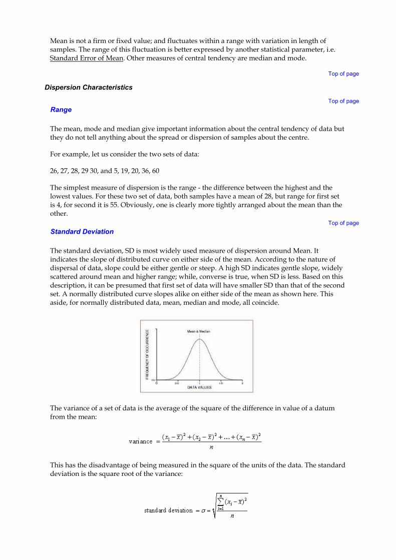
The variance of a set of data is the average of the square of the difference in value of a datum from the mean:

This has the disadvantage of being measured in the square of the units of the data. The standard deviation is the square root of the variance:

This formula with denominator 'n' indicates SD of entire population. However, for all practical purposes, we deal with 'samples' only, and in such case, denominator 'n' is replaced by (n-1) to account for limited length of data. Excel formula to estimate this parameter is =stdev(Range of data). Here, for two sets of data, SD computed is 1.58 & 21 respectively, which is consistent with our presumption made earlier.

Top of page

Skewness

In several cases, frequency of occurrence of variables is not normally distributed and plots either skewed +ve (right) (as shown in the fig.) or skewed -ve (left). In other words, slopes of the curve on either side are dissimilar. Unlike normally distributed data, mean, median and mode for skewed data do not coincide. Peaked point of skewed plot is the location of mode. For normally distributed curve, skewness is zero.

This parameter is determined by function skew(range of data) in MS Excel. It is evident, from table, that for evenly distributed data set, skewness is zero. Second set of data is positively skewed.

HEC-SSP software itself computes these parameters and performs a number of tasks using them.

Top of page

WHICH VALUE/DATA QUALIFIES AS AN ANNUAL PEAK OF A YEAR ?

Collection of a set of particular type of data is purpose driven. For frequency analysis of flood peaks corresponding to a return period of 50-yr or so, we look for collection of a set of instantaneous peak discharge of different years. Here, instantaneous peak discharge of a year means that discharge is highest of all discharge values flowed past a measuring section during the period. The question is how to gather this set of information. Following Para discusses this aspect.

Hourly discharge observation is not only expensive but also impracticable. Instead, a widely prevalent practice in India is to record discharge observation once a day (usually at 0800hr or so), and water level every hour. It is important to note that recorded discharge observation may or may not be the peak discharge of the day; and therefore, it can't be a true representative of an instantaneous peak discharge of a day. Let us understand it differently. In a plot shown here, water level hydrograph and the level when discharge was carried out have been shown together. It is easily noticeable here that peak water level (hence discharge) occurred between two observations. This means that if we pick up instantaneous peak discharge out of observed discharge recorded in a year, missing out true instantaneous peak can't be ruled out. Therefore, it had better look for all such peaks in a year, and pick up a corresponding discharge value that is highest of all. Followings are few approaches suggested to consider before finalizing an array of annual peaks.

1. Fit a rating curve (s) between observed discharge and corresponding water level. Rating curves so developed and hourly water level hydrograph together can be used to obtain a no-break/continuous discharge series of a particular year. A plot of water level and continuous discharge series, developed using HYMOS software, is displayed here. Peak of this series represents instantaneous annual peak of that year.

2. In absence of rating curve, a correlation between past observed discharge or mean daily discharge (maximum of a year) and instantaneous peak discharge can be developed. This relationship can be used to generate peak discharge corresponding to maximum observed discharge for subsequent years.(for detailed discussion, pl refer to Hydrologic Frequency Analysis, Vol-3 published by US Army Corps of Engineers- 1975, http://www.hec.usace.army.mil/publications/IHDVolumes/IHD-3.pdf )

3. In some quarters, peak daily or peak mean daily discharge data are raised by certain

percentage, say 20 or 30%. This method is little ambiguous and subjective as all peak daily values may or may not touch instantaneous peak by application of a certain percentage.

Top of page

HOW TO ENSURE FITNESS OF DATA FOR FREQUENCY ANALYSIS?

Annual peaks gathered for frequency analysis must be a product of random factors only. Presence of one or more data influenced by manual and/or systematic errors gravely distorts the distribution of plot and its reliability, if go unnoticed in the analysis. So, it is essential that a suspected data should be detected and treated for its modification or retention or deletion before analysis. This apart, data should possess attributes, such as homogeneity, randomness, and stationarity. These attributes are explained in succeeding paragraphs.

a. Homogeneity

Homogeneity implies that the sample is representative of same population. The homogeneous requirement means that each flood occurs under more or less similar conditions. Two flood events are homogeneous, if both are caused by same factor, such as rainfall. Flood peaks triggered by dam break, breach in embankment are isolated events, and should not be part of peaks created by rainfall. It is assumed that though peak flows of finite years' have been recorded; the same type of 'Statistical Character' (mean, standard deviation, and skewness) was always there and would behave alike in future too. For this reason, a set of data belonging to same population must closely exhibit the similar statistical behaviour with another set of data of same population. To test homogeneity of data, Student 't' test is normally performed.

b. Independence/Randomness

This is explained in previous module on this topic. Independence or randomness is usually investigated by Turning Point test.

c. Stationarity

In this the properties or characteristics of the sample do not fluctuate with time. Linear trend test determines this property of sample.

If any of these is not an attribute of a sample, the use of probability/theoretical frequency distribution may lead to erroneous results. Accordingly, it is desirable that before any analysis, one must see that sample should conform to these attributes.

HEC-SSP offers no tools to perform these tests. Nevertheless, interested users, can use HYMOS software to test if compiled set of data qualifies for flood frequency analysis.For more details, we recommend reference to Hydrology Project-I Training Module no.43. This material is available as part of this week's module.

Top of page

EMPIRICAL Vs. THEPRETICAL DISTRIBUTION CURVE

Absolute frequency - Supposing there is a variable which can take values from 0 to 100. A sample of this variable holds 50 different values. Let us group these data in five equal intervals, e.g., 0-20, 20-40,--- -- --, 80-100. There distribution across five groups is 'absolute frequency'. Absolute frequency, say n divided by N, is relative frequency or probability. Please notice that sum total of relative frequency is '1'. This concept is used a little later.

A relative frequency curve plotted on the basis of distribution of data in a sample presents a distribution curve known as empirical distribution curve. This distribution and its statistical parameters help an engineer fit a theoretical frequency distribution curve, as closely to the empirical distribution as possible to ensure mathematical tractability further.

Fig 1

As understood a while ago, the probability or relative frequency is defined as the number of occurrences of a variate divided by the total number of occurrences, and is usually designated

by P(x). The total probability for all variates should be equal to unity, that is, �P(x) = 1. Distribution of probabilities of all variates is called Probability Distribution, and is usually denoted as f(x) as shown in Fig.1.

The cumulative probability curve, F(x) is of the type as shown in Fig.2.

Fig 2

The cumulative probability or 'probability of non-exceedance', designated as P(x < x), represents the probability that the random variable has a value less than certain assigned value x. Additive

inverse of P(x < x), or P(x � x), is termed as Exceedance Probability. Reciprocal of exceedance

probability is return 100 times the Exceedance Probability is called as Exceedance Frequency. Now, glance at Table1; and read what the probability of 60 not getting exceeded is.

Table 1

In the context of flood frequency analysis, we apply above concepts by assuming the instantaneous yearly flood peaks as the variate 'x'. Then, if the functions f(x) or F(x) becomes known by fitting a theoretical distribution, it is possible to find out the probability (or return period) of a flood peak, or conversely, a flood magnitude of desired return period (also return interval or recurrence interval).

There are a number of probability distribution functions f(x), which have been suggested by statisticians. HEC-SSP supports following distribution functions.(Reader can download and install HEC-SSP software from site, http://www.hec.usace.army.mil/software/hec-ssp/downloads.html )

Without log transformation

With log transformation

Another often used distribution is Gumbel method. Even if, HEC-SSP software does not include this method, user can readily use mean and standard deviation to estimate flood peak corresponding to a return period, T = (1/P) by use of formula placed below:

XT = M + B * (-ln (-ln (1-P)))

Where,

However, this method is recommended when length of data is fairly large, say more than 100 (ref: Patra K C, Hydrology and Water Resources Engineering). Alternatively, when data is scarce, i.e., data length is below 100, user may use Gumbel table, which features in almost every hydrology book, to read K, frequency factor for given sample size and return period. In this case, X

Tis estimated by

XT= Xmean + K * St Deviation

I. Normal &

II. Pearson type III

I. Log normal &

II. Log Pearson type III

M = Xmean

- 0.45005 * Standard Deviation

B = 0.7797 * Standard Deviation

Top of page

PLOTTING POSITION

To assign a probability to a sample data (also called variate) and to determine its 'plotting position' on probability sheet, sample data consisting of N values is arranged in descending order. Each data (say the event X) of the ordered list is then assigned a rank 'm' starting with 1 for the highest up to N for the lowest of the order. The exceedance probability of a certain value x is estimated by formula presented below:

p = (m-a)/(N-a-b+1)

Where, m is rank of the sample data in the array; N represents the size of sample; and 'a' and 'b' are constants. For different methods, a and b assume different values. For Weibull method, a & b equal zero; and hence, P reduces to m/(n+1). HEC-SSP, by default, uses Weibull method to show dispersion of data. Nevertheless, option is available for alternate methods by defining appropriate value of a & b. Of these, the Weibull formula is most commonly used, because it is simple and intuitively easily understood to determine the probability. (For detailed discussion on the choice of a particular method, reader may refer to Applied Hydrology by Ven T Chow, p - ).

Top of page

WHICH DISTRIBUTION FITS WELL ?

HEC-SSP offers graphical plot displaying scatter of sample data in addition to computed curve. Here, user has choice to choose method of plotting position and a theoretical curve of his choice. Graphical plot is a visual aid of determining worthiness of choice broadly; and therefore, conclusion based on merely eye judgment is hugely subjective. To overcome this limitation, user can analyze the result distilled by software and employ any one of the following tests to measure the strength of fitness. However, such analysis needs to be done outside; as HEC-SSP contains no built-in function of this kind. This module presents steps to perform D-test only. Details with regard to others, users may refer to Hydrology Project Training Module no.43.

� Chi-square test� Kolmogorov-Smirnov test� Binomial goodness of fit test, and� D-index test

Once a particular distribution is found the best, it is adopted for calculation of peak floods in future.

D-index is calculated by

where,

D-index test is shown later in this module.

D-index = ����1to6 (abs(Xiobserved

- Xicomputed

)/(mean of sample)

Xi observed

= observed value of a given p, exceedance probability

Xi computed

= for identical p, value determined by distribution curve

Top of page

CASE STUDY

This point forward, a real sample (Table 2) has been collected for its frequency analysis with HEC-SSP software. The application of the method of plotting and fitting a theoretical distribution curve, analysis of output will help reader grasp the functions of this software speedily. The software outputs a series of additional information, which have been discussed at appropriate locations.

Step 1

As quoted earlier, this set of data is required to be investigated to confirm its adherence to

desired attributes of sample data, i.e. homogeneity, randomness and stationarity. Following is screenshot of HYMOS software which is used to conduct series homogeneity test of a given series. A pop-up window in the middle of this screenshot indicates results of this series as 'accepted'. In all three tests, hypothesis, that series is random, is not rejected. This implies that the current sample is a collection of random data.

Step 2

Subsequent steps begin with creation and saving of an EXCEL sheet with two columns - first for year and second for discharge. This file is imported (Fig.4) in HEC-SSP software to carry out frequency analysis. Interested reader is suggested to go through 'User's Manual' of this software (p 4-7 to p 4-9 to learn how to import data from MS excel), which is available under 'Help' menu of software.

This manual is also available at http://www.hec.usace.army.mil/software/hec-ssp/documentation/HEC-SSP_20_Users_Manual.pdf .

Optionally, user can directly input data by selecting 'Manual' button on 'Data Importer' window (Fig.4). To open 'Data importer' window, click on 'Data' menu followed by choosing 'New'.

Fig 4

Step 3

Once, data is available, Chapter 6 of 'User's Manual' help user finish frequency analysis. 'General Frequency Analysis Editor' window as shown in Fig.5 can be activated by selecting Analysis New - General Frequency Analysis option on the menu. An analysis report (Table 3) along with distribution curve (Fig.6) generated by the software for this set of data using Log Pearson type III distribution is placed next. Before, we delve into results; let us familiarize ourselves with a couple of lines appearing on the plot. Later, we will discuss their significance, and how they are estimated.

Tiny circular points in blue are annual peaks occupying their position on the plot (also probability sheet) according to probability assigned to them by 'Weibull method'. As discussed earlier in the module, this scattering is 'Empirical Frequency Distribution'. A line in red denotes Log Pearson Type-III 'Theoretical Distribution Curve'. Could you read on the plot what return period for circular point farthest to the right is? It is roughly 30yrs. If we desire to ascertain peak discharge of still higher return period sticking to empirical distribution, no information is available. For a majority of hydrological and hydraulic related studies, flood magnitude of return period of 50 yrs or more is needed. Such estimations are extracted with the help of theoretical distribution plot, which is mathematically extended further.

Fig 5

� A dotted line in blue is expected probability curve. This aspect is discussed later.� A pair of two lines in green on either side of plot is 90% confidence band. This aspect is

also covered later.

Table 3

Of several useful contents generated by software, two of them need special attentions.These are:

I. Confidence Limits, and

II. Expected Probability

Top of page

CONFIDENCE BANDS AND CONFIDENCE LIMITS

The record of annual peak flow at a site is a random sample collected over a period of time. A varied nature of causative factors and complex interactions among them bring about randomness in the sample. Therefore, in all likelihood, a different set of samples of same population results in different estimate of the frequency curve. Thus, an estimated flood frequency curve can be only an approximation to the true frequency curve of the population of annual flood peaks. To gauge the accuracy of this approximation, one may construct an interval or a range of hypothetical frequency curves that, with a high degree of confidence, contains the population frequency curve. Such intervals are called confidence intervals and their end points are called confidence limits. This is analogous to standard error of mean or standard error of mean relationship concept.

The two limits of 0.05 and 0.95, or 5% and 95% chance exceedance curve,(pl see the result in table 3), imply that there is 90% chance/probability that discharge value will lie/occur between these bounds; and only 10% of observation may fall outside this band. If we put it differently,

upper limit suggests a flow with 5% of exceedance probability, or (100-95), i.e. 5% non-exceedance probability. If certainty of this degree is warranted for any project, flow of this magnitude can be chosen for design, but at the cost of escalation in project cost. In fact, this choice is a trade-off between cost of the project and safety of the structure. Similar conclusion can be drawn about lower limit

The confidence band width is determined by a formula given below:

QU,L

= Qmean

± KU,L

* St Deviation

Where,

KU,L

is a function of exceedance probability, sample size, skewness coefficient and confidence

interval opted by the user. The value of KU,L

declines with rise in sample size. This brings two

lines representing QU & QL closer to each other, and therefore, a narrower band will appear. HEC-SSP assumes exceedance probability of 0.05 and 0.95 by default and returns the output. User, at his discretion, can select any other value instead. For more details about K

U, L, reader

may refer to 'Reference 2'.

Top of page

EXPECTED PROBABILITY

The expected probability adjustment is necessitated to account for a bias introduced in the distribution curve on account of shortness of data. Factually, all distributions assume spread of

data from - to + ; while in reality, this is far from real. This calls for measures to address short length of data. Table 4 is an excerpt from Applied Hydrology by Ven Te Chow listing correction factors for different return periods.

Where, N is number of sample data used in the analysis. Please notice that as N approaches infinity, expected probability equals exceedance probability. Here too, HEC-SSP offers both alternatives to compute or not to compute expected probability and corresponding flood values for various exceedance probabilities (Fig.7).

Top of page

HOW TO PERFORM D-INDEX TEST

HEC-SSP software, by default, outputs flood peaks of a few exceedance frequencies like 0.2, 0.5, 1.0, 2.0, 5.0, 10.0, 20.0, 50.0, 80.0, 90.0, 95.0, and 99.0. However, appropriate part of window, shown at Fig.8, can be suitably adjusted by the user to gather flood peaks of desired exceedance frequency, usually matching with what tabulated by the software using Weibull method. (pl refer to tabular result under Table 3).

An attempt to compute D-index values for this set of data, outside the HEC-SSP environment, is placed at Table 5. Please mark that data, as highlighted in red in Table 3, populate this table for calculation of D-test. It could be seen, lower the value of D-test, the better the fit is.

Top of page

OUTLIERS

Outliers are values in a data set which plot significantly away from remainder of sample data (main body of the plot), and their deletion, retention and modification warrants prudent considerations of all of the factors giving birth to them. In Paragraph to follow, this aspect has been discussed at length.

The following equation is used to detect outliers:

QHigh, QLow = Qmean ± KN * St Deviation

Where,

HEC-SSP automatically performs detection process; reports and analyzes the set of data accordingly.

KN

is a frequency factor and varies according to sample size.

Top of page

HANDLING DIVERSE SCENARIOS

The study covered in this module plots all annual peaks more or less closely aligned to theoretical distribution line (see Fig.6). It also means the absence of even a single peaks straying from rest of peaks. So, the number of outlier for this case is zero. Nevertheless, samples not as coherent as cited here are always a possibility; and it is likely that they may contain outliers -both high and low or either of the two; i.e. zero flows; or even historical floods outside the systematic (also continuous) records of annual peaks.

In dealing with such records, one, however, must be convinced about the authenticity of data, and should guard against entries of all inflated or dubious values in the analysis.

In HEC-SSP, presence of zero flows and low outliers are automatically detected and counted out by the software, and a conditional probability adjustment, to account for truncated values, is employed to estimate revised plotting position. Software also modifies values of statistical parameters to define theoretical distribution curve.

In a deviation from above, high outliers, so long as they are not suspected values, are not eliminated from the record as they are invaluable piece of the flow record and might be representative of longer period of record. For example, a flood value in a set of data, detected by software as outlier, could be the largest flood that has ever occurred in an extended period of time backward. Like other cases, HEC-SSP detects high outlier as well, and presents the analysis accounting for revised length of time period entered by user and number of high outliers detected by software itself. A computed curve returned by the software utilizes modified statistical parameters, i.e. mean, standard deviation, and skewness coefficient. Fig.9 is one of the windows of the software that lets user make appropriate entry to define Historical Period, if a high outlier falls beyond the systematic record. To gather more information about mathematical steps involved in dealing with varying cases such as cited here, interested users should refer to material referenced against Sl. No. 2, at the end of this chapter.

Here, we place sample data set (Table 6 & 7) for Flood Frequency Analysis under different conditions. User may key in this set of data in HEC-SSP to perform frequency analysis for different cases.

As outlined in one of the preceding paragraphs, HEC-SSP has the ability to detect low outliers and/or zero flows and projecting the probability curve by introducing conditional probability adjustment. Contrary to this, analysis of high outliers and historical data do need a few entries by user. Fig.10 deals with high outliers, where a peak discharge of 71,500 cumec is labeled as a high outlier by software, and an entry of 1892 by user in a cell by start year implies this peak is highest known value since year 1892. Fig.11 deals with historical data; where user has entered historical flood value along with corresponding year. An entry of 1974 against end year signifies no significant flood since regular discharge recording ceased in year 1955.

Top of page

REFERENCES

1. HEC-SSP User's Manual, available at http://www.hec.usace.army.mil/software/hec-ssp/documentation/HEC-SSP_20_Users_Manual.pdf

2. Guidelines for Determining Flood Flow Frequency- Bulletin 17B of the Hydrology Sub-Committee - A publication by US Department of the Interior Geological Survey Office of Water Data Coordination, http://water.usgs.gov/osw/bulletin17b/bulletin_17B.html

3. Ven Te Chow, David R Maidment, Larry W Mays, (International Edition 1988), Applied Hydrology, McGraw-Hill Book Company

4. Patra, K C, (2001), Hydrology & Water Resources Engineering, Narosa Publishing House5. Hydrologic Frequency Analysis, Vol-3 published by US Army Corps of Engineers- 1975,

http://www.hec.usace.army.mil/publications/IHDVolumes/IHD-3.pdf 6. Mutreja, K N, Applied Hydrology, Tata McGraw Hill Publishing Company Limited, N

Delhi

7. Hydrology Project- Phase I (India), Training Module no.43

Top of page

CONTRIBUTOR

Anup Kumar Srivastava

Director

National Water Academy, Pune, India

Top of page

ACKNOWLEDGEMENT

Author of this module hereby acknowledges the invaluable support received from Shri D S Chaskar, and Dr R N Sankhua, both Directors, National Water Academy, CWC, Pune in preparation and presentation of this module in current shape.