Statistical Methodology for Profitable Sports Gambling

by Fabián Enrique Moya

B.Sc., Anáhuac University, 2001

Project Submitted in Partial Fulfillment of the Requirements for the Degree of

Master of Science

in the Department of Statistics and Actuarial Science

Faculty of Science

Fabián Enrique Moya 2012 SIMON FRASER UNIVERSITY

Summer 2012

All rights reserved. However, in accordance with the Copyright Act of Canada, this work may be reproduced, without authorization, under the conditions for “Fair Dealing.” Therefore, limited reproduction of this work for the

purposes of private study, research, criticism, review and news reporting is likely to be in accordance with the law, particularly if

cited appropriately.

ii

Approval Name: Fabián Enrique Moya Degree: Master of Science

(Applied Statistics) Title of Project: STATISTICAL METHODOLOGY FOR

PROFITABLE SPORTS GAMBLING

Examining Committee: Chair: Dr. Carl Schwarz, Professor

Dr. Tim Swartz Senior Supervisor Professor

Dr. Paramjit Gill Committee Member Professor, Department of Mathematics and Statistics University of British Columbia – Okanagan

Dr. Joan Hu External Examiner Professor

Date Defended/Approved: July 24, 2012

iii

Partial Copyright Licence

The author, whose copyright is declared on the title page of this work, has granted to Simon Fraser University the right to lend this thesis, project or extended essay to users if the Simon Fraser University Library, and to make partial or single copies only for such users or in response to a request from the library of any other university, or other educational institution, on its own behalf or for one of its users. The author has further granted permission to Simon Fraser University to keep or make a digital copy for use in its circulating collection (currently available to the public at the "Institutional Repository" link of the SFU Library website (www.lib.sfu.ca) at http://summit.sfu.ca and, without changing the content, to translate the thesis/project or extended essays, if technically possible, to any medium or format for the purpose of preservation of the digital work. The author has further agreed that permission for multiple copying of this work for scholarly purposes may be granted by either the author or the Dean of Graduate Studies. It is understood that copying or publication of this work for financial gain shall not be allowed without the author's written permission. Permission for public performance, or limited permission for private scholarly use, of any multimedia materials forming part of this work, may have been granted by the author. This information may be found on the separately catalogued multimedia material and in the signed Partial Copyright Licence. While licensing SFU to permit the above uses, the author retains copyright in the thesis, project or extended essays, including the right to change the work for subsequent purposes, including editing and publishing the work in whole or in part, and licensing other parties, as the author may desire. The original Partial Copyright Licence attesting to these terms, and signed by this author, may be found in the original bound copy of this work, retained in the Simon Fraser University Archive.

Simon Fraser University Library Burnaby, British Columbia, Canada

revised Fall 2011

iv

Abstract This project evaluates the performance of betting systems using as many real-life elements as possible. Starting with a gambling record of more than 600 bets that were actually placed at an online sports gambling website, a Monte Carlo simulation is carried out to compare different bet selection strategies and staking plans. The best performing system is identified and its performance is measured taking into account the actual constraints found in online sports gambling; finally, the results are measured with respect to a 40,000 customer database from the same bookmaker where the bets were placed. The results offer compelling evidence that a finely tuned sports betting system involving a solid selection process and optimized staking has the potential to produce large profits with a limited initial bankroll after a relatively short amount of time.

Keywords: Betting systems; Kelly criterion; Monte Carlo simulation; Online gambling; Probability; Statistical analysis.

v

Dedication To my beloved wife, Marcela. You are the love of my life.

To my beloved daughter, Michelle. You are the joy of my life.

Para Marcela, mi esposa amada. Eres el amor de mi vida. Para Michelle, mi hija amada. Eres la alegría de mi vida.

vi

Acknowledgements I would like to thank a number of people who supported me in every conceivable way during my graduate studies at Simon Fraser University. I would not have been able to successfully complete my Master’s without their help.

I will always be indebted to Dr. Tim Swartz, my senior supervisor. Thank you for taking an interest in me and for always believing in my academic ability. I am also particularly thankful to Robin Insley for trusting in me as a workshop teaching assistant and coordinator. But above all, thank you to both of you for your sincere friendship.

I’d also like to express my deepest gratitude to my friend, Prof. Dante Campos. It was his exceptional commitment to teaching that gave me the required foundation to undertake the rest of my graduate studies. Although it wasn’t fun at that time, I truly appreciate all those long study nights spent with me reviewing statistical theory. Also, the words and advise of Darby Thompson (err, I mean Dr. Thompson) were truly invaluable. Thank you for coping with my never-ending novel of hesitation in that particularly challenging first semester. I am also very grateful for the financial support and crude but immensely helpful advise I received at that time from Dr. Derek Bingham. As he predicted my life indeed sucked for four months but I appreciate how he always looked for a solution to every problem I brought up to him despite his lack of available time back then.

I am thankful to Ian Bercovitz for challenging my writing skills and for giving me the opportunity to step up in front of a classroom to teach statistics. I would also like to thank all the professors whose class I had the chance to take and that cared for my learning, and most specially to Dr. Tom Loughin for teaching the one statistics course that I truly enjoyed and that showed me that there is indeed a light at the end of the tunnel.

I am also grateful for the many lifelong friendships I have forged here. Kasra, thank you for such a great friendship, for listening to my frequent rants about life

vii

and what not, and for sharing your thoughts, your cookies and your tea with me. Andrew, despite the fact that you are unbelievably obnoxious I want to thank you for developing my thoughts from purely logical to truly scientific, and for inspiring and supporting me to grow in statistical programming ability. Nate, thank you for making me part of your vision of the future, for offering your unconditional help before I even asked for it, and for lending me a hand in my transition to Canada.

I can’t also overlook my “IRMACS buddies”, particularly Jack, Megan, Rachel and María. A special mention in this group goes for Alberto Contreras for his completely unselfish support at a time I needed it. Thank you for regarding me as one more of your buddies!

I also want to say ‘thank you’ to all the students I met (and hopefully helped) at the statistics workshop. More than once your comments gave me confidence in myself and my own ability. Your questions, endlessly repeated every semester, were for me a humble reminder of where I once stood as a student in this discipline.

There are also a few very special people that supported me by taking care of my family while I was away. I have a deep gratitude to Mrs. Tavita García and Mr. Javier Zavala, my ever caring parents-in-law. Thank you for providing for my beloved girls, I will always keep that appreciation in my heart. And to my brother from another mother, Javier, thank you for taking care of Michelle as the bestest possible uncle. God bless you always.

But there are no words that could ever describe how much I thank you, Marcela, because this accomplishment would not have been possible without your love, your support, your patience, your tears, and the everyday sacrifices you underwent while I was away from you. I owe it all to you, and I hope I can repay you by giving you my heart, my soul, and my entire life by your side. We will never be apart again.

viii

Table of Contents Approval........................................................................................................................ ii Partial Copyright Licence............................................................................................iii Abstract ........................................................................................................................ iv Dedication ..................................................................................................................... v Acknowledgements ..................................................................................................... vi Table of Contents .......................................................................................................viii List of Tables ................................................................................................................ ix List of Figures................................................................................................................ x

1. Introduction to Sports Gambling ............................................................... 1 1.1. Similarities and Differences Compared to Traditional Gambling .................... 1 1.2. Evolution of Contemporary Sports Gambling.................................................... 2 1.3. Sports Gambling Terminology ............................................................................ 4 1.4. Motivation for the Project ................................................................................... 6 1.5. Organization of the Project ................................................................................. 7

2. Online Sports Gambling: Exploratory Data Analysis ................................ 9 2.1. The Global Online Gambling Market.................................................................. 9 2.2. Profits and Losses of Online Sports Gamblers ................................................. 10 2.3. Performance of a Winning Sports Gambling System ...................................... 15

3. Performance Assessment of Sports Betting Systems................................18 3.1. Constraints in real-life sports betting ............................................................... 18 3.2. Sports betting systems ....................................................................................... 19 3.3. Staking plans ...................................................................................................... 21

3.3.1. Fixed (level) staking ............................................................................... 21 3.3.2. Percentage staking ................................................................................. 22 3.3.3. Kelly staking............................................................................................ 22 3.3.4. Other staking plans ................................................................................ 24

3.3.4.1. Fixed-Profit staking.................................................................. 24 3.3.4.2. Progressive staking .................................................................. 25 3.3.4.3. D’Alembert staking .................................................................. 25

3.4. Monte Carlo Simulation of Betting Systems ..................................................... 26

4. Discussion...................................................................................................33

Bibliography.......................................................................................................35

ix

List of Tables Table 1. Monetary performance of online bettors ................................................ 12

Table 2. Author’s Gambling Record (AGR), sample of ten data points. ................ 16

Table 3. Simulation results, fixed stakes staking................................................... 28

Table 4. Simulation results, full fractional Kelly staking. ..................................... 29

Table 5. Simulation results, half fractional Kelly staking. .................................... 30

Table 6. Simulation results, half fractional Kelly staking with staking limits. ......................................................................................................... 31

x

List of Figures Figure 1. Worldwide gross gambling revenue, and online gambling break-

up. .............................................................................................................. 10

Figure 2. Histogram of average stake amount per bet (euros / bet). ..................... 13

Figure 3. Histogram of total amount wagered by online gamblers (euros). ......... 14

Figure 4. Histogram of net profits and losses of online gamblers (euros)............. 15

Figure 5 Histogram of final bankrolls, half Kelly staking with maximum stake limit. ................................................................................................. 32

1

1. Introduction to Sports Gambling

1.1. Similarities and Differences Compared to Traditional Gambling Sports gambling is a form of betting similar to traditional probability games

such as roulette, dice, or cards. The result of a sports bet is settled based on the outcome of a sporting event on which none of the betting parties has any influence. In traditional gambling, the probability of events can be calculated exactly, whether the number of possible results is small (as in flipping a fair coin) or very large (picking five cards out of a standard deck of 52 cards.) In traditional gambling, probabilities are based on the symmetry definition of probability. In contrast, the probabilities for the outcomes of a sporting event can’t be calculated exactly. These probabilities are subjective and can only be estimated by previous similar occurrences and other factors influential to the sport and the players involved.

In the game of roulette, a gambler may choose among different types of bets, such as a straight (bet on a single number), a corner (bet on four numbers), a dozen (a bet on the first, second, or third group of twelve numbers), or the color the roulette will show (red or black). These events have different probabilities of occurring and therefore have different payouts associated to them. In the previous examples, the straight bet has the higher payout (36 times the amount wagered) while a winning bet on the roulette color will only double the amount originally risked. However, all the outcomes have a negative expectation from the point of view of the gambler, because the payouts are calculated as if the roulette had 36 pockets when in reality there are 37 or 38 possible outcomes. This difference is known as the house edge or vigorish, and it provides the expected profit of the casino over a long number of roulette spins.

2

Betting on the result of sporting events has a similar structure. The gambler may choose between the different outcomes, which are specific to every sport: the winner of a tennis match (two outcomes), the result of a soccer game (three outcomes as draws are possible) or first place of a horse race (many possible outcomes). However, as already stated, the probabilities for all of the possible outcomes are not exactly known, so the house has to come up with its own estimate for them. It will then offer payouts according to those estimates, but slightly adjusting them down for every selection to provide the house edge. The goal for the house is to manage its payout liabilities properly so that it secures a profit regardless of the final outcome of the sporting event. Again, this difference is the house edge over the gambler and provides the expected profit after a series of sporting events. It is important to note that sports gambling uses its own terminology and definitions for many of these concepts, but are kept unchanged to allow a direct comparison.

1.2. Evolution of Contemporary Sports Gambling Although gambling on sports outcomes has existed for a long time in many

societies, it could be argued that its development has mirrored that of organized professional sports. In its simplest form sports gambling is usually conducted at the venue of the event itself, and thus it has a regional flavor. That’s the way horse racing wagering evolved in the UK in the late nineteenth century, and cockfighting is still conducted in many countries around the world. The advent of newspapers first, and TV a few decades later, enabled people to place bets on the final outcome of many events taking place throughout the world. Some countries introduced legislation aimed to regulate a growing industry, while some other countries completely outlawed sports gambling. Even in those countries where sports gambling is allowed, a special government license is typically required to own and operate a sports betting business.

The twentieth century also saw the rapid development of several professional and nonprofessional sports leagues. In North America the most notable examples are the NFL (American football), the NBA (professional

3

basketball), MLB (baseball), NHL (ice hockey), and even the NCAA (university-level sports). Many of the top European soccer leagues have also grown dramatically, such as La Liga (Spain), Serie A (Italy), Bundesliga (Germany), the Premier League (England), and Ligue 1 (France), along with Europe-wide competitions such as the UEFA Champions League. Some sports developed a series of international competitions that attract large crowds. Tennis features four yearly Grand Slams, rugby has a World Cup, the Six Nations Championship, and the Continental Nations Cup. And cricket went as far as to develop new competition formats, such as One Day Internationals (ODIs) and Twenty20, to attract larger audiences. As a result there’s a large number of sporting events going on all over the world all year-round, catering to many different tastes.

The final piece of contemporary sports betting came into place with the arrival of online gambling. Before online gambling arrived sports gambling houses offered odds on a relatively small number of offerings, catering to the largest possible audience. For example, in the UK gambling was mostly focused on horse racing and soccer. Additionally, the house usually offered a handful of options for each sporting event. For example, for a regular football match a gambler could only try to predict the winner of the match, the number of goals (over or under a certain threshold), and sometimes the halftime/fulltime combined outcome.

When gambling houses went online they had to cater to a global audience and therefore they started offering odds on many more events. However, nothing prevented the house from making these new events available to every gambler registered on the website. Just like a gambler from Iceland could place a bet on the English Premier League, a Scottish gambler could place a bet on an Indian cricket tournament with the same ease. Furthermore, the gambling houses greatly expanded the number of offerings to bet on for every event. For example, currently a single soccer match can have more than a 100 possible offerings to wager on: the score at halftime, the team to score first, the team to receive more yellow cards, the team to win the coin toss, etc. Finally, technology developments made it possible to place bets while the match is in progress, which is referred to as in-running or live betting. When a meaningful event happens in the match the

4

odds are recalculated on the fly, so gamblers can literally place a bet at the last minute.

1.3. Sports Gambling Terminology As previously mentioned, sports gambling has developed its own

terminology to refer to many of the most important concepts.

• Bookmaker: The bookmaker, also called the bookie or simply ‘the house’, it refers to the business or organization that provides an odds market for sporting events, with prices available for all possible outcomes. A “book” is simply the full record of all betting transactions made with the bettors for a particular event.

• Event: This refers to the specific sporting event. Examples of events are India vs Sri Lanka playing the final of the Cricket World Cup or Real Madrid playing against Barcelona in the Spanish Soccer League.

• Market: A betting market is a type of betting proposition with two or more possible outcomes. The result of the match (home win, away win, or draw), the number of goals scored (two or less goals, three or more), or the time of the first goal are a few examples of different markets for a single sporting event.

• Bank: the total amount of money a gambler has to place bets on sporting events.

• Stake: the amount of money being risked in a single bet.

• Odds: In the context of sports gambling the odds of an outcome refer to the payout to be received if a prediction turns out to be correct. In this project the European notation for odds will be used. This notation describes the amount of money returned for every dollar wagered,

5

including the original stake. For example, a bet that offers a profit equal to the amount wagered is said to have odds of 2; an outcome with offered odds of 5 describes a profit of four times the amount wagered, while an outcome with odds of 1.20 means that for every dollar gambled the bet will return only 20 cents in profit, assuming in all the cases the wager was correct.

• Fair odds: the odds that would be offered if the sum of the probabilities for all possible outcomes were exactly 1 (100%). For example, supposing we had a market with three possible outcomes {A, B, C} with probabilities of success P(A) = 0.5, P(B) = 0.4 and P(C) = 0.1, the fair odds would be 2.00, 2.50, and 10.00 respectively, which are just the inverse of the estimated probabilities.

• Overround: Also called vigorish (or vig for short) in American sports betting, the overround is a measure of the bookmaker’s edge over the gambler. The bookmaker will never offer fair odds on a market. In practice, the payout offered on each selection will be reduced, which in turn increases the reflected probability of an event. When odds have been adjusted in this way the sum of the probabilities for all events will exceed 1 (100%). The overround is the amount by which the sum of all probabilities exceeds 100% and it is the bookmaker’s profit margin. For example, if we had a market with two possible outcomes {A, B}, where P(A) = P(B) = 0.5, the fair odds on each selection would be 2.00. However, the bookmaker may offer payouts of 1.85 on each selection. The corresponding probabilities for each selection are now 1/1.85 = 0.5405, and the sum of the probabilities for all outcomes is 0.5405 x 2 = 1.081. The overround is 8.1%, and for every $100 paid out by gamblers the bookmaker expects to make a profit of 8.1 dollars, assuming that there are balanced bets on both A and B.

• Pick: The selection among all the possible outcomes on which the gambler is placing the bet.

6

• Result: The actual outcome of the event. If the pick and the result are the same the gambler wins the bet and is paid an amount equal to his stake times the odds offered on the selection. If the result is different from the pick the gambler loses his entire stake.

• Profit: The amount of money additional to the original stake that the gambler receives when the bet is won. Bookmakers sometimes use the term Winnings, but this term refers to the amount of money paid back including the original wager, which is somewhat misleading. It is preferable to speak about the profit made in a bet instead of the winnings of a wager.

• Yield: A measure of the profitability of a series of bets, it is calculated as the sum of the profit made from all the placed bets divided by the sum of the money staked in all bets, usually expressed as a percentage. For example, if after 10 bets of $1 each there is a net profit of $1.50, the yield is (1.5/10) = 0.15 � 15%.

1.4. Motivation for the Project When the bookmaker offers odds on a particular market, it is implicitly

making estimates of the probabilities for the different outcomes. It is possible that the bookmaker might make inaccurate probability estimates for some markets. If a gambler can identify incorrectly assessed markets it may then be possible to turn sports gambling into a positive expected value activity.

In the 2006 FIFA World Cup I was able to identify one niche market where an online bookmaker routinely made inaccurate probability estimates. Big events like the World Cup attract many new potential gamblers, and bookmakers usually increase the number of available markets. One soccer market offered odds on the exact number of additional minutes to be played at the end of each half (referred to as ‘injury time’), which is usually displayed on an electronic board at the end of the regulation time. The bookmaker decided to estimate the probabilities (and

7

therefore the odds) of each possible outcome by looking at historical averages, and then offered these “averaged odds” across all events regardless of other factors. I speculated (correctly) that the most important factor for estimating the outcome of this market is the central referee of the match. It is well known in soccer that referees have different personalities that affect their refereeing style, and I thought that this trait would also have an impact on the additional time to be played. I just needed data to justify my intuition.

Unfortunately, aggregate injury time is only routinely recorded for one tournament, the UEFA Champions League. The data initially available from this source wasn’t enough to accurately profile individual referees (most referees had ten or fewer observed matches), so I manually recorded the injury times for almost every soccer match played in the most important European leagues for one year. These records, coupled with the initial data collection, allowed me to identify some referees whose distribution of injury time was different enough from the average to generate positive expected value betting propositions. So at the start of the 2007-08 European soccer seasons, I decided to place a bet every time I identified one of these opportunities. During that season I placed more than 250 bets which resulted in a respectable profit.

At that time I also became concerned with some additional questions: what is the most profitable staking strategy? Can the betting selection process be improved? Will the probability of success increase if the bets are placed in-running instead of the beginning of the match? Can I use a similar methodology in more mainstream markets, like match results or over/under goals scored? Back then I dealt with these questions with only an intuitive feeling for statistics. This project will explore these issues in a more rigorous way, using statistical tools and techniques which have been acquired during my M.Sc. studies.

1.5. Organization of the Project In chapter 2, I will present a detailed overview of internet sports betting as

an economic activity from the point of view of the gambling industry. I will also

8

present a real life dataset featuring a summary of online gambling behaviour of 40,000 people to analyze gambling profits and losses at an individual level. An exploratory data analysis will be conducted on this dataset to assess the typical behaviour of online gamblers. Finally, I will introduce my own gambling record as an example of a profitable sports betting system, which will be used extensively throughout this project.

In chapter 3, I propose and investigate various gambling strategies associated with my dataset. Issues such as when to bet and how much to bet are the key elements of chapter 3. The Kelly system is introduced as an “optimal” method of wagering. However, I observed that there are limitations associated with the Kelly system. I conclude with a short discussion in chapter 4, where I argue that some combination of Kelly and common sense is optimal.

9

2. Online Sports Gambling: Exploratory Data Analysis

2.1. The Global Online Gambling Market The gross gaming revenues (betting stakes less gambler winnings) of the

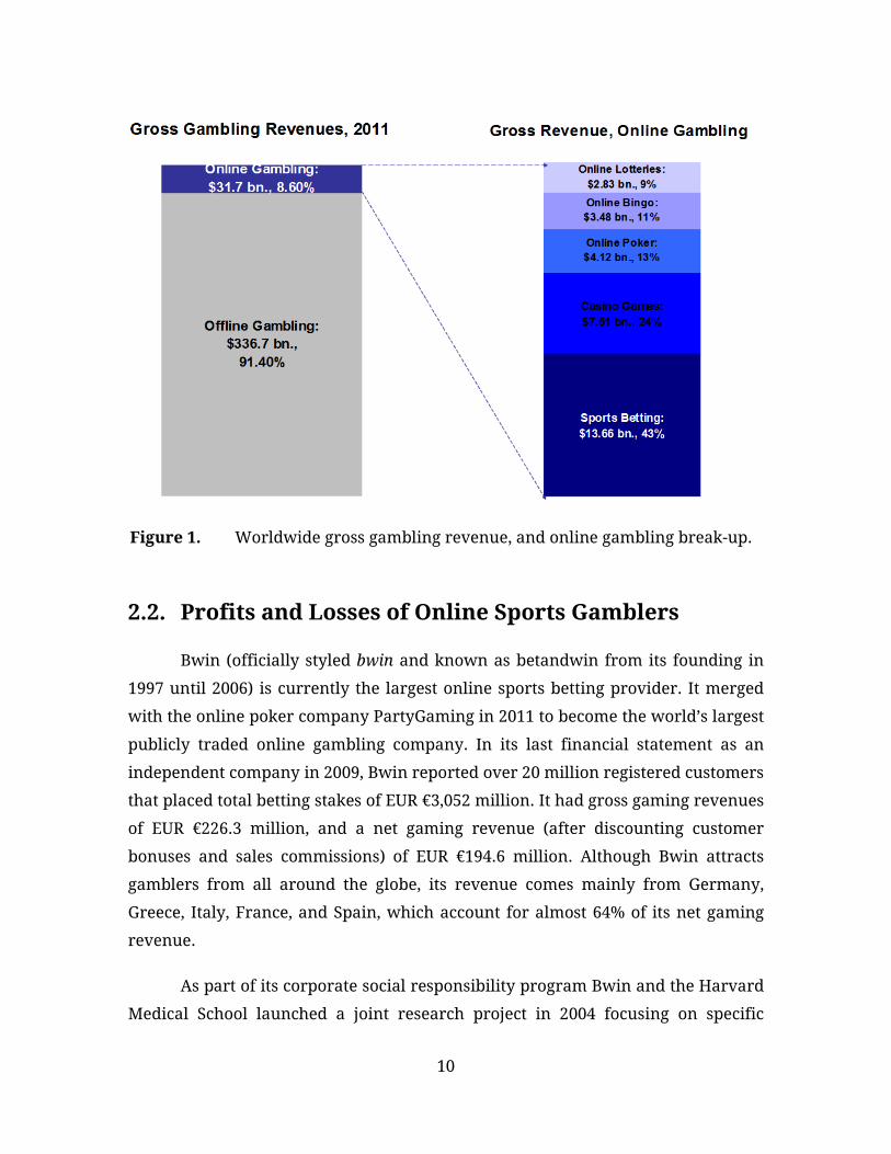
global gambling industry (both online and offline) reached EUR €286 billion (CAD $368.4 billion) in 2011. The online gaming sector accounted for 8.6% of the revenue, amounting to EUR €24.6 billion (CAD $31.4 billion). This amount encompasses not only sports gambling but also all the sectors of internet gambling, namely online versions of poker, casino games, bingo, and traditional lotteries. Sports betting is the largest sector, accounting for 43% of all online revenue. Thus, internet betting on sports is a market of approximately EUR €10.6 billion (CAD $13.66 billion) (H2 Gambling Capital, 2012). Figure 1 graphically describes revenue in the worldwide gaming industry.

Europe accounts for the largest single share of the global interactive market with 44% of the value being derived from the region in 2011. Furthermore, 14.4% of the European gambling sector's gross revenues were generated via interactive channels in the mentioned year. (H2 Gambling Capital, 2012.) From this point onward this project uses mostly European gambling conventions, such as using Euros as the main currency, and referring to gambling odds in European format (as opposed to the American format or English odds).

There were just over 2,600 real money Internet gambling sites offered by about 660 parent companies (operators) in 2010, with 150 such sites created within that year alone. The average gross win per operator was EUR €35.5 million. Over the same period the average gross win per site was EUR €9.1 million (H2 Gambling Capital, 2011).

10

Figure 1. Worldwide gross gambling revenue, and online gambling break-up.

2.2. Profits and Losses of Online Sports Gamblers Bwin (officially styled bwin and known as betandwin from its founding in

1997 until 2006) is currently the largest online sports betting provider. It merged with the online poker company PartyGaming in 2011 to become the world’s largest publicly traded online gambling company. In its last financial statement as an independent company in 2009, Bwin reported over 20 million registered customers that placed total betting stakes of EUR €3,052 million. It had gross gaming revenues of EUR €226.3 million, and a net gaming revenue (after discounting customer bonuses and sales commissions) of EUR €194.6 million. Although Bwin attracts gamblers from all around the globe, its revenue comes mainly from Germany, Greece, Italy, France, and Spain, which account for almost 64% of its net gaming revenue.

As part of its corporate social responsibility program Bwin and the Harvard Medical School launched a joint research project in 2004 focusing on specific

11

features of Internet gaming. Bwin provided a dataset with information representing eight months of aggregated betting behaviour data for 40,499 sports betting subscribers who opened an account during the period from February 1, 2005 through February 27, 2005. LaBrie et. al (2007) initially used the dataset to conduct research on gambling addiction but the dataset can also be used to characterize the actual profit or losses incurred by online gamblers. The subject of this chapter is the investigation of the nature of betting habits.

The dataset records separately variables related to fixed-odds bets and live-action bets. Fixed-odds bets are those placed before the start of sporting events, as opposed to live-action bets, which are placed while the event is taking place. The original terminology will be respected for consistency purposes but for this project the distinction between fixed-odds and live-action bets is not relevant and the betting records will be analyzed pooling both types of bets together where possible.

A total of 5.3 million fixed-odds bets were placed for a turnover (total stakes gambled) of EUR €29.0 million. The gamblers in the dataset cumulatively lost EUR €3.8 million, for an average loss of 13.1% on monies staked. This is an interesting observation since the vigorish on fixed-odds bets (see Chapter 1) is around 10%. This may suggest that odds are slightly “tilted” to attract losing bets. In addition, online gamblers in this cohort also placed 2.46 million live-action bets for total stakes of EUR €32.6 million. Total gamblers’ losses for this type of bet were EUR €2.1 million, or 6.4% of stakes. Taken together, the average gambler’s loss during this period was 9.6% of total stakes. This percentage is a direct measure of the profitability of the bookmaker and it is actively managed, as reported in Bwin’s 2005 annual report: “Sports betting involves a significantly greater risk for the gambling house than poker and casino games, where stable margins can be achieved at comparatively low risk. Inadequate bookmaking expertise may also translate into the inability to achieve the desired margins. In the field of sports betting it is betandwin’s goal to achieve gross winnings margins within a bandwidth of 8% to 10%. The company reported a gross winnings margin of 8.7%

12

for sports betting in the year under review, compared with 9.9% in the financial year 2004.” (Betandwin, 2006)

Table 1 reports some summary statistics based on the Bwin dataset without distinction between fixed-odds and live-action bets. The large difference between the mean and the median, coupled with large standard deviations and a wide range of values, result from a highly skewed distribution for the three indicators. Taken together, these results suggest that most gamblers conduct bets with small sums of money, together with a few “high rollers” that gamble, win, and also lose, much larger amounts.

Table 1. Monetary performance of online bettors Mean Median SD Minimum Maximum

Euros / Bet 12 4.6 31 0.4 1,000 Total wagered 1,522 197 8,479 0.4 440,103 Net return -147 -41 792 -26,824 38,310 Note: Figures are in euros. Negative values indicate gambler’s losses (n = 40,499)

Figure 2 provides a histogram for the amount staked per bet. It can be observed that the average amount gambled in a single bet goes from less than half euro per bet all the way up to 1,000 euros, the maximum amount allowed by Bwin on a single bet. However, the median is a much more modest EUR €4.60, and the 90th percentile (not shown in Table 1) is EUR €24.25. In fact, the distribution has such a long tail that is not informative to present it in full. However, if we limit the stake size to €30 euros or less it is possible to appreciate some interesting features. The distribution of average individual wagers is roughly exponential, with the addition of a batch of “penny bets”, and “bumps” every €5 euros. It is likely that these regular increases stem from gamblers that stake a fixed amount on every bet.

13

Figure 2. Histogram of average stake amount per bet (euros / bet). Note: Only gamblers whose average stake is less than or equal to €30 are shown (n =

37,321)

The variability among individual gamblers is even more pronounced for the total amount wagered (the sum of all bets placed by the bettor), as shown in Figure 3. The standard deviation is more than five times the size of the mean, and the median amount of €197 is much lower than the average of €1,522, indicating the presence of outliers. An inspection of the raw data reveals that, on the one hand, many players placed only a few bets with low total stakes. Alternatively, there are a few highly active bettors. For example, the gambler that placed the maximum total stake of €440,000 made more than 3,600 bets, suggesting that he placed between 20 to 40 daily bets of about €120 each when he actively gambled.

14

Figure 3. Histogram of total amount wagered by online gamblers (euros). Note: Only values less than or equal to €2,000 are shown (n = 36,184)

Figure 4 presents the net winnings or losses for online gamblers in the cohort. The mean return is a loss of around €150. However, this result exhibits great variability too as the standard deviation is also more than five times the (absolute) value of the mean. It is interesting to note that the median is -€40, showing that most sports bettors end up losing money, albeit a relatively small amount. However, next to those moderate losers are individuals who lost many thousand of euros as well as some other bettors that achieved similarly outstanding profits. Again, the vast differences in financial performance suggest wildly different types of bettors present in the sample. It is also worth noting the increases in frequency for some round values, suggesting that many gamblers stop playing once they reach a self-imposed loss limit, as is particularly evident at -€100. The proportion of gamblers that achieve any profit is notoriously small, providing evidence for the difficulty of overcoming the negative expectation of gambling odds with overround.

15

Figure 4. Histogram of net profits and losses of online gamblers (euros). Note: Top and bottom 2,600 observations removed (n = 35,299)

These results show, unsurprisingly, that the most common outcome for the sports gambler is to incur a monetary loss. However, the bwin dataset allows us to quantify the amount of these losses using real life data. Moreover, it can also be used as a benchmark to gauge the performance of sports betting systems.

2.3. Performance of a Winning Sports Gambling System From September 8, 2007 to September 13, 2009 I placed around 600 bets in

the market for injury time in soccer as described previously. Throughout this project I will refer to this dataset as the author’s gambling record, or AGR.

Table 2 presents a sample of ten bets from the AGR. Every record in the AGR describes a placed bet and it is given a unique ID. The next four variables use abbreviated names to describe the football match: the tournament (also called league) in which the match was played, the home and away teams, and the officiating referee. The variable HALF indicates whether the additional time prediction was made for the first or second half. The next variable PICK denotes the number of extra minutes corresponding to the wager. The next two variables,

16

FREQ and SUPP, represent the number of times the wagered outcome had been previously observed for the appointed referee, and the total number of observations registered for the referee at that moment in time. The PROBEST variable is simply the percentage of frequency to support, and it is essentially a probability estimate. The ODDS at which the bet was placed were also recorded, not only to calculate the eventual payoff, but also to provide the bookmaker’s probability estimate for the outcome. The EDGE is the difference between the personal probability estimate and Bwin’s probability estimate (the reciprocal of ODDS in percentage terms.) Finally, the last variable RESULT states the eventual outcome of the bet.

Table 2. Author’s Gambling Record (AGR), sample of ten data points. ID LEAGUE HOME AWAY REF HALF PICK FREQ SUPP PROBEST ODDS EDGE RESULT 282 UCL CHELS BARCA OVRT 1 2 mins 10 14 71.43% 3.50 42.86% 3 mins 283 UEFAC HAMB WBREM BLEF 2 3 mins 23 29 79.31% 2.70 42.27% 3 mins 284 ITA.A SAMP REG TREM 2 5 mins 8 51 15.69% 16.50 9.63% 0 mins 285 ITA.A SIENA PALRM CIAM 2 5 mins 5 9 55.56% 11.00 46.46% 6 mins 286 ESP.1 VALLD NUMNC CLOG 2 3 mins 7 10 70.00% 4.05 45.31% 3 mins 287 ESP.1 OSAS SEV VELC 1 2 mins 6 13 46.15% 4.00 21.15% 1 min 288 ESP.1 OSAS SEV VELC 2 3 mins 5 7 71.43% 3.42 42.19% 3 mins 289 ENGPL CHELS BBURN STYR 2 2 mins 11 28 39.29% 4.50 17.06% 2 mins 290 UEFAC SHAKD WBREM MEDC 2 2 mins 15 66 22.73% 11.40 13.96% 3 mins 291 ESP.1 BILB ATMAD PERB 1 2 mins 24 46 52.17% 4.00 27.17% 1 min

The main attribute to explore in the AGR is the expectation of profit. However, the AGR contains only bets that were actually placed at the sports book. There were additional matches where Bwin offered the injury time market but no bet was placed, and the odds offered in those instances were not recorded in the AGR. This information would have been useful to assess the proposed betting systems. The analysis is therefore restricted to those predictions recorded in the AGR that met the criteria explained in section 3.2.

The AGR dataset is divided in two parts mirroring the European football season, which runs from August to May of the following year. Therefore each one of these parts is called a season; the first part is the 2007-08 season (or simply the

17

first season), while the second part is the 2008-09 (or last) season. Both seasons were profitable, although the performance of the second season is much better than the first season. A total of 289 bets were placed during the 2007-08 season, with stakes of about EUR €20,500 and a net profit of EUR €3,500; the average amount staked per bet was therefore €70 and the total yield was 17.5%. The 2008-09 season staked EUR €19,500 over the course of 306 bets for a final profit of EUR €7,800; the average stake per bet was around €64 euros yielding a 40% profit over the amount staked. The next chapter will explore alternative betting strategies with respect to the AGR dataset.

18

3. Performance Assessment of Sports Betting Systems

3.1. Constraints in real-life sports betting There are two ways of analyzing gambling in favourable games: one of

them involves (mostly) analyzing their mathematical properties on simplified models, characterizing their asymptotic behaviour and finding generalizable results. This project, however, analyses favorable games in a constrained, real life setting. Some of these constraints are:

• The true probability of a successful wager is unknown: This is the most important limitation. The research on favourable games assumes that either the true probability of success or the edge over the expected value is known. However, as previously stated, that assumption isn’t met when bets are placed on sports outcomes.

• Bank is finite: Although this seems to be an obvious remark, it is possible to have a gambler with infinite resources, for example, a casino extending an unlimited line of credit for a finite amount of time (Thorp, 1969). Unfortunately I wasn’t one of those clients.

• Gambler plays a finite number of times: Formally, a game is considered favorable if there is a gambling strategy such that the bank becomes infinite as the number of bets goes to infinity. For this project we are more concerned with strategies where the final bank balance is greater than the initial bank after a fixed (and relatively small) number of n trials.

19

• Odds are not the same for all events: A common simplifying assumption is to consider games where trials are independent and identically distributed (and therefore offering the same payout in each trial). While there are sports betting markets where this assumption holds (i.e., handicap markets), the bets analyzed in this project were placed over a relatively large range of odds.

In addition, there are additional constraints placed by the bookmaker:

• Minimum stake size: Systems that rely on staking a fraction of the available bank (to be explained later) assume that money is infinitely divisible (Breiman, 1961). In real life the bookmaker requires a minimum amount to be wagered and therefore the risk of bankruptcy, that is, running out of gambling funds, can never entirely be removed.

• Winning limits: The bookmaker usually sets a maximum allowed bet. The maximum protects the bookmaker from large adverse runs and in particular prevents gamblers from ensuring profits by ‘doubling up’ (staking increasingly large amounts of money after unsuccessful bets in order to cover the previous losses and make a profit on top of that). Bwin has a limit of €1,000 on the returns (original stake plus profit) of a single bet.

3.2. Sports betting systems If the true probability of success is not known and the bookmaker offers an

artificially reduced payout, a natural question arises: Is it possible to identify favourable betting propositions? Moreover, is it possible to consistently achieve profit from sports gambling?

The published literature reports some instances of series of sports bets with profitable outcomes and statistical robustness (Clarke et al, 2008; and Direr, 2013.) One common element of these papers is the presence of a bet selection process.

20

This process explores all available bets within a market and selects a subset of bets to gamble on according to a set of rules. These rules are of varying complexity, ranging from statistical models such as the logistic regression model for baseball outlined by Insley et al (2004), or can be as simple as a cutoff rule based on available odds in soccer, as presented by Direr (2013).

Nevertheless, past performance is routinely used as the main predictor for future results, and such data form the basis of much of the fixed odds compilation by the bookmakers. The key to gaining an edge over the bookmaker then becomes an issue of finding better and more relevant data with which to build a more accurate forecasting model for sports prediction. Coming up with a bet selection process that identifies betting edges for the gambler on a regular basis is notoriously difficult, albeit not impossible.

Once the gambler has identified bets with positive expectation, it is necessary to determine how much money to gamble on each wager. It is possible for gambler in a favorable game to lose money, and even to go bankrupt, if the stake amount is not properly set. A staking plan is the set of rules that determine the amount of money to stake in each bet. Different staking plans may have different goals, such as maximizing profit, minimize risk of bankruptcy, or minimize bank variance. The stake amount is limited by the total available funds to gamble, as well as the minimum and maximum amounts allowed by the bookmaker.

For this project a sports betting system is defined as the combination of a bet selection process with a staking plan. As previously mentioned the market selected to place bets was additional (injury) time in soccer matches. Ignoring some of the details, personal estimates were derived by observing the relative frequency of the outcomes in each referee’s previous appearances. The bet selection process consisted in placing a bet when the personal probability estimate of one outcome differed from Bwin’s implied probability estimate by 10% or more. The AGR is the inventory of all bets placed under this condition. The rest of the chapter will explore the profit performance of different staking plans.

21

3.3. Staking plans Initially, it would seem that the goal of a gambler is to maximize the amount

of his/her bank B after a finite but unknown number of n wagers (trials). However, the expected payoff in a system with positive expectation is maximized by betting the total bank on each trial, and thus, one single loss leads to ruin (bankruptcy). The probability of this event approaches 1 as the number of bets is increased, and therefore maximizing expected profit is undesirable (Thorp, 1969).

In light of this result the gambler may wish to minimize the probability of bankruptcy. It can be shown (Thorp, 1969) that in a favorable game, the chance of ruin is decreased by decreasing stakes and therefore this probability is minimized by making a minimum bet on each trial. However, this strategy has the undesirable consequence of also minimizing the expected profit. The gambler then needs an intermediate staking strategy between minimizing ruin and maximizing profit, and some options will be explored in the context of the AGR.

3.3.1. Fixed (level) staking Fixed staking, also called level staking, is the simplest of staking plans. In it,

every bet placed is assigned the same stake, regardless of any other consideration. The gambler must only decide the amount of the stake, which is usually stated as a percentage of the initial bank (instead of the current bank after a number of bets.) The main disadvantage of this strategy is that it doesn’t take into account any additional information such as the current bank, the odds offered by the bookmaker, or the estimated edge size.

If the current bank is less than the initial bank, the fixed stake size represents a larger proportion of the total bank and therefore a larger risk of bankruptcy. On the other hand, if the balance has increased after a number of bets the stake size is now a smaller percentage of the total available funds and therefore potential profits are forfeited. Additionally, it is evident that a bet placed at odds of 10 has a smaller probability of occurring than a bet with odds of 2. Common sense would suggest to use a smaller stake for the riskier bet. Conversely,

22

a bet with a larger edge over the bookmaker would suggest a bigger stake than one with a reduced edge value.

Nonetheless, level staking forms the benchmark staking strategy against which all others should be compared for profitability and risk evaluation (Buchdal, 2003).

3.3.2. Percentage staking This staking strategy fixes the percentage of the current bank at the time the

bet is placed, rather than a proportion of the initial bankroll. Therefore the stake size will fluctuate with the size of the available bank. This system addresses one of the shortcoming of level staking, and profits are gradually increased above those for level stakes when the edge is positive, but it still ignores the edge size, which is undoubtedly a critical piece of information.

In situations with positive expectation the total amount wagered in percentage staking will eventually be much greater than in level staking and it will generally outperform it, while at the same time the risk of ruin is greatly reduced. However, when losses are made the strategy calls for reduced stakes, increasing the time it takes to recover the initial bankroll when compared to simple level staking. This is not a trivial issue, as percentage staking may be potentially more profitable and theoretically safer than level staking over the long term, but it is less likely to show a profit in the short term. This tradeoff has significant implications for the psychology of real-life betting (Buchdal, 2003).

3.3.3. Kelly staking The Kelly staking strategy resembles percentage staking, but the proportion

of the bankroll to gamble varies on each bet. In the context of information theory, Kelly (1956) determined that a gambler should not aim to maximize the expected profit for each bet (as previously explained) and instead should seek to maximize the expected log of the payoff. This approach makes perfect sense because it is equivalent to maximizing the rate of growth of profit. A few years later, Breiman

23

(1961) generalized Kelly’s calculations to outcomes that result from a mix of a number of finite distinct distributions, each occurring on a given trial with a specified probability. In addition, Thorp (1969) extended the use of the Kelly formula to settings such as the stock market, where probability estimates are uncertain but gamblers can nevertheless find bets with positive expectation. These two extensions allow the use of Kelly’s formula in a sports betting scenario where the probabilities for the different outcomes can only be estimated and the wagering odds might change from one bet to the next.

Kelly (1956) showed that there is an optimal percentage of the bankroll to bet in favourable games. This percentage varies according to the edge the gambler has over the bookmaker. Given a bet selection process that identifies an outcome with probability of success 0 < p < 1, and European odds θ > 1, the optimal betting fraction of the bankroll given by Kelly (1956) is

1*

1

pf

θθ

−=

− (1)

provided that p > 1/ θ.

Kelly staking has some remarkable asymptotic properties: gambling the optimal fraction will cause the bankroll to increase infinitely. Kelly staking will also “dominate” any other staking plan, meaning that gambling the Kelly fraction will yield higher expected returns than any other strategy. Conversely, gambling the optimal Kelly fraction will minimize the expected time required to achieve a specific bankroll goal, e.g., doubling the initial bank.

It is particularly interesting to note the effects of wagering percentages other than the optimal Kelly fraction. Staking plans that gamble less than the optimal fraction will also cause the bankroll to increase infinitely, albeit more slowly. However, gambling more than the optimal Kelly fraction will eventually led to bankruptcy. Therefore, the Kelly criterion penalizes overbetting much more heavily than underbetting.

24

Kelly staking has its own drawbacks. Although it is asymptotically optimal, a bankroll may experience considerable reductions in the short term with just a few losses. In particular, if the estimated edge is large the Kelly criterion might require betting a large portion of the bank at once, which obviously leads to a large loss if the bet isn’t successful. It is worth remembering that the probability of an outcome can only be estimated for sports gambling; it might be possible that a bet selection process provides reasonable estimates in situations with small to medium edges together with a few situations where the edge is overly optimistic. It might also be possible that the true probability of success of an event changes suddenly. For example, if a new regulation is introduced, this can lead to a miscalculation in the edge.

One way to minimize these risks is to gamble only a fraction of the stake indicated by the Kelly criterion. A common choice is the “half Kelly” staking plan, where the optimal Kelly fraction is multiplied by 0.5. Half Kelly has 3/4 the growth rate of the full Kelly but has a much less chance of a big loss (Thorp, 2006). Most people strongly prefer the increased safety and psychological comfort of “half Kelly” in exchange of 1/4 of the growth rate (Thorp, 2006), myself included.

3.3.4. Other staking plans There are other staking plans that are sometimes mentioned in the

gambling literature. These staking plans involve increasing or decreasing the stake size after each bet, according to whether it won or lost, with a view to recovering earlier losses or enhancing gains whilst on a winning run. A brief description is given here for the sake of completeness, but they won’t be considered in this project. Any gambler seriously interested in profiting from sports gambling would not use any of these plans. However, the curious reader might want to review Buchdal (2003) for an in-depth discussion of these systems and their shortcomings.

3.3.4.1. Fixed-Profit staking The gambler fixes the amount he wants to win in every successful bet. If all

the bets were placed at the same odds this strategy would amount to level staking.

25

However, where the odds differ, the stake sizes will vary. The logic for this plan is to increase the stake for those bets that have a higher probability of success, and reduce the stake for those bets that are less likely to be successful. This staking plan is particularly vulnerable to situations where a very likely outcome actually fails to materialize. This strategy doesn’t take into account the current bankroll and the edge size.

3.3.4.2. Progressive staking This staking plan comes from casino gambling, and in particular from

roulette betting where the payoff is the same as the amount staked (odds of 2.00). The initial goal is to win a small profit with the first bet. However, if this bet is unsuccessful, the goal of every subsequent bet is to recover the money that has been lost up to that point, plus the original target profit, returning to the original stake size once a bet is won. At odds of 2.00 the progressive staking strategy calls for doubling the staked amount after a losing bet.

The fatal flaw of the progressive strategy is that a run of several consecutive losses quickly increases the required stakes until it eventually surpasses the maximum betting limit or the gambler’s bankroll. At this point the gambler is left with a huge loss that usually wipes out any previous profits.

3.3.4.3. D’Alembert staking Also called the Pyramid plan, in its simplest form it also assumes an even

payoff (odds = 2.00). An initial stake is gambled, and if the bet is unsuccessful the initial stake is added to the current wager. In the case of a losing run the increase in stakes is arithmetic (1, 2, 3, 4,…) instead of geometric (1, 2, 4, 8,…). After a bet is won, the stakes are decreased according to the same arithmetic pattern. When the gambler reaches the original stake he is assured a profit equal to the original stake.

Although clearly less aggressive than progressive staking, the D’Alembert staking plan could require an infinite number of bets after a losing streak to “return” the point where a profit is made. That is, every losing bet requires an equal number of winning bets afterwards to materialize the profit.

26

In theory, progressive staking “works” because it wins with probability one regardless of the value of p. In D’Alembert staking the system must have an edge to return with probability one to the original stake.

3.4. Monte Carlo Simulation of Betting Systems In order to measure the performance of sports gambling systems, it isn’t

enough to be satisfied with the betting record. The history of placed bets is just one instance of all possible betting histories due to the inherent randomness in sports results. A profitable record can’t assess on its own the inherent probability of profit, or to end up in bankruptcy. Furthermore, the variation in offered odds and stake amounts renders simple probability distributions like the binomial ineffective. Instead, this project will use Monte Carlo simulation.

The simulation will test the performance of several sports betting systems, that is, different combinations of staking plans and bet selection criteria. Recall that the AGR is the inventory of all bets derived from a bet selection process that required an edge (a positive difference between the personal probability estimate of an outcome and Bwin’s implied probability estimate) of 10% or larger to place a bet. However, the gambler might want to test the accuracy of his estimates over a range of all the edges that were obtained. Changing or restricting the range of the edge required to place a bet effectively creates different bet selection criteria. It is plausible to think that too large an edge is in reality an indication of an unknown, influential factor. If that were the case there would be a cluster of lost bets hidden among the overall profitability of the bet selection process. It is also plausible to think that too small an edge may negatively affect probability. Therefore, restricting the edge for qualifying bets might remove losing bets and increase overall profitability.

In the AGR the estimated edge ranges from 10% to 63%, and the edge is divided into four groups based on this range: bets with an estimated edge of 10% up to 20%; 20% up to 30%; 30% up to 40%; and more than 40%. The simulation will test ten possible bet selection criteria stemming from the possible combinations of

27

ranges available at these cutoff points. In addition the simulation will initially test three different staking plans: fixed stake, “full” Kelly, and “half” Kelly. It should be noted that initially the simulation will enforce the minimum stake restriction to allow for the possibility of bankruptcy, but it won’t enforce the restriction on the maximum amount allowed wager to showcase the theoretical properties of the different staking plans.

Each simulation proceeds as follows: A total of 200 bets are sampled at random and without replacement from the AGR. Please note that the bets can be sampled in any order and that it is possible to sample bets whose edge might not be accepted under any of the selection rules. Each bet selection criteria identifies the subset of qualifying bets from the sample and wagers starting with an initial hypothetical bankroll of €100. The wagering process is done using three staking plans: fixed stakes, full fractional Kelly, and half fractional Kelly. For each simulation and betting system the number of bets, the final bankroll and the yield are recorded. The simulation is repeated 10,000 times, and then the following statistics are calculated: average number of qualifying bets, mean final bankroll, standard deviation of the mean final bankroll, probability of profit (the proportion of simulations where the final bankroll is greater than the initial bankroll), 10th and 90th percentile of the mean final bankroll, and average yield.

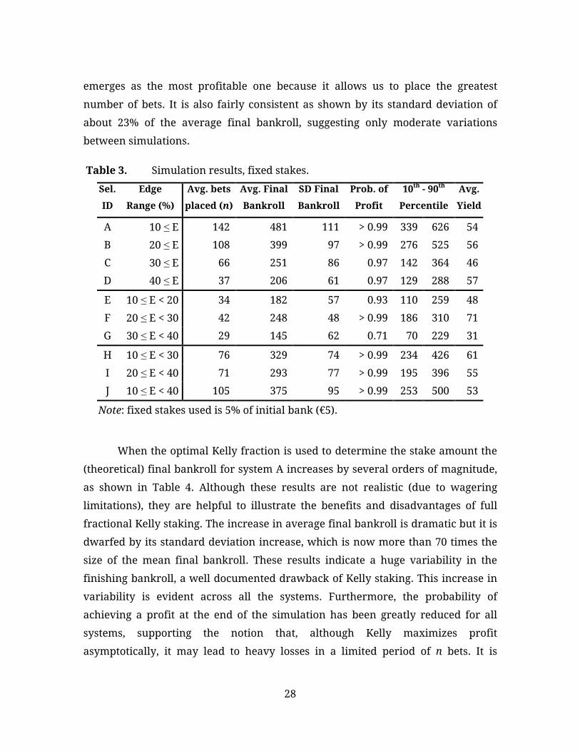
Table 3 presents the result of the different betting systems using fixed stakes. As previously mentioned this staking plan is the benchmark against which to compare other staking strategies. Systems D, E, F, and G represent the four selection strategies discussed previously, and each system places a similar number of bets on average. The four edge ranges are profitable, confirming the gambler does have an edge over the bookmaker, and that the edge exists regardless of the edge range. In terms of yield systems F and G are the most profitable and least profitable respectively. It is worth noting they represent two adjacent edge ranges. All systems show a great probability of profit with the notable exception of system G, providing further evidence that the estimated edge in the range of 30% to 40% is not as strong as it is in other ranges. System G is also the only one whose 10%-90% percentile range covers a bankroll loss region. Based on these results system A

28

emerges as the most profitable one because it allows us to place the greatest number of bets. It is also fairly consistent as shown by its standard deviation of about 23% of the average final bankroll, suggesting only moderate variations between simulations.

Table 3. Simulation results, fixed stakes. Sel. ID

Edge Range (%)

Avg. bets placed (n)

Avg. Final Bankroll

SD Final Bankroll

Prob. of Profit

10th - 90th Percentile

Avg. Yield

A 10 ≤ E 142 481 111 > 0.99 339 626 54 B 20 ≤ E 108 399 97 > 0.99 276 525 56 C 30 ≤ E 66 251 86 0.97 142 364 46 D 40 ≤ E 37 206 61 0.97 129 288 57 E 10 ≤ E < 20 34 182 57 0.93 110 259 48 F 20 ≤ E < 30 42 248 48 > 0.99 186 310 71 G 30 ≤ E < 40 29 145 62 0.71 70 229 31 H 10 ≤ E < 30 76 329 74 > 0.99 234 426 61 I 20 ≤ E < 40 71 293 77 > 0.99 195 396 55 J 10 ≤ E < 40 105 375 95 > 0.99 253 500 53

Note: fixed stakes used is 5% of initial bank (€5).

When the optimal Kelly fraction is used to determine the stake amount the (theoretical) final bankroll for system A increases by several orders of magnitude, as shown in Table 4. Although these results are not realistic (due to wagering limitations), they are helpful to illustrate the benefits and disadvantages of full fractional Kelly staking. The increase in average final bankroll is dramatic but it is dwarfed by its standard deviation increase, which is now more than 70 times the size of the mean final bankroll. These results indicate a huge variability in the finishing bankroll, a well documented drawback of Kelly staking. This increase in variability is evident across all the systems. Furthermore, the probability of achieving a profit at the end of the simulation has been greatly reduced for all systems, supporting the notion that, although Kelly maximizes profit asymptotically, it may lead to heavy losses in a limited period of n bets. It is

29

pointless to discuss the relative merits of the different systems under this setting as it is clear that full fractional Kelly staking is too risky for most gamblers.

Table 4. Simulation results, full fractional Kelly staking. Sel. ID

Edge Range (%)

Avg. bets placed (n)

Avg. Final Bankroll

SD Final Bankroll

Prob. of Profit

10th - 90th Percentile

Avg. Yield

A 10 ≤ E 142 125187888 8982299453 0.69 0 1064064 4 B 20 ≤ E 108 15783951 922243791 0.63 0 290563 3 C 30 ≤ E 66 57793 1480357 0.30 0 2857 -8 D 40 ≤ E 37 22289 340404 0.44 0 6644 -2 E 10 ≤ E < 20 34 668 1445 0.78 56 1564 21 F 20 ≤ E < 30 42 43463 284587 0.98 499 82170 43 G 30 ≤ E < 40 29 254 1797 0.24 0 369 -14 H 10 ≤ E < 30 76 293740 3573464 0.99 884 359384 35 I 20 ≤ E < 40 71 65718 642557 0.80 24 57169 13 J 10 ≤ E < 40 105 441006 7001915 0.86 51 219565 13

Scaling down the full fractional Kelly corrects many of the previous disadvantages, as illustrated by the results in Table 5, where only half of the optimal Kelly fraction was used to determine the stake size. Although there is still a great deal of variability in the average final bankroll, the probability of profit at the end of the simulation is back to very high levels for all but the worst performing selection process. Under an optimized staking strategy such as half Kelly, system A has widened the performance gap it had over all other systems. Achieving the highest mean final bankroll and a 99% probability of profit is enough evidence to conclude system A is the best selection process. However, these theoreticized profits are completely fictitious because the maximum stake limit set by the bookmaker was not taken into account.

30

Table 5. Simulation results, half fractional Kelly staking. Sel. ID

Edge Range (%)

Avg. bets placed (n)

Avg. Final Bankroll

SD Final Bankroll

Prob. of Profit

10th - 90th Percentile

Avg. Yield

A 10 ≤ E 142 897248 10285236 0.99 1061 777219 25 B 20 ≤ E 108 304999 3044813 0.97 532 310565 25 C 30 ≤ E 66 12454 113284 0.81 44 15376 14 D 40 ≤ E 37 4771 23279 0.86 67 8694 21 E 10 ≤ E < 20 34 296 251 0.88 91 589 32 F 20 ≤ E < 30 42 2829 4194 > 0.99 402 6345 54 G 30 ≤ E < 40 29 251 514 0.51 20 568 2 H 10 ≤ E < 30 76 8262 18087 > 0.99 699 18640 46 I 20 ≤ E < 40 71 6539 19598 0.96 195 14448 28 J 10 ≤ E < 40 105 19116 78473 0.98 372 38155 29

Finally, Table 6 show the performance of the different bet selection processes using the half fractional Kelly staking plan accounting for the bookmaker limits on stake size: the minimum stake size is €1, and ruin occurs when the bankroll falls below this amount. The maximum possible stake plus profit is €1,000, so once a staking plan reaches this limit it essentially becomes a fixed profit plan.

Under real life conditions the performance of system A is remarkable, achieving an almost hundredfold mean average increase in bankroll, a 99% percent probability of profit and a 90% probability of multiplying the initial bankroll by a factor of 14. A key element is the large number of bets placed, as this allows the multiplying nature of the staking strategy to kick in and greatly increase profit. Another point worth highlighting is the performance difference between systems B and J, the second and third best performing systems. Both strategies have a similar number of bets placed on average, suggesting that their performance difference is due to the inclusion of bets with an edge greater than 40%, which are part of system B but not of system J. The evidence suggests that the

31

edge estimation is accurate even in those instances when the estimation process produces a large perceived edge.

Table 6. Simulation results, half fractional Kelly staking with staking limits. Sel. ID

Edge Range (%)

Avg. bets placed (n)

Avg. Final Bankroll

SD Final Bankroll

Prob. of Profit

10th - 90th Percentile

Avg. Yield

A 10 ≤ E 142 9703 5697 0.99 1489 17148 29 B 20 ≤ E 108 7316 4900 0.98 638 13892 29 C 30 ≤ E 66 1977 2342 0.82 45 5481 15 D 40 ≤ E 37 1720 1931 0.86 68 4612 23 E 10 ≤ E < 20 34 296 250 0.88 91 590 32 F 20 ≤ E < 30 42 2258 1966 > 0.99 402 5191 55 G 30 ≤ E < 40 29 232 379 0.51 20 565 2 H 10 ≤ E < 30 76 4193 3116 > 0.99 703 8698 47 I 20 ≤ E < 40 71 2739 2771 0.96 196 7012 29 J 10 ≤ E < 40 105 4545 3863 0.98 380 10132 30

Figure 5 summarizes the final bankroll results for system A under complete realistic conditions. It is interesting to note that the distribution of bankrolls is bimodal, but that one of the peaks is at the leftmost bin. My interpretation is that a sequence that starts out losing takes time to recover and it results in a slump of low profits. However, if the initial bets placed are successful the profit expands with a long right tail.

32

Figure 5 Histogram of final bankrolls, half Kelly staking with maximum stake

limit.

33

4. Discussion The procedure outlined in the previous chapter serves as a blueprint to

evaluate and optimize sports betting systems. As explained, the hardest part is to actually come up with a bet selection process with positive expectation. Monte Carlo simulation using fixed level staking is a very powerful tool to test different bet selection processes. Since this technique is based on sampling from observed instances it is important to record as many observations as possible, including cases without advantage to the gambler. In this project the analysis of the bet selection process would have been much richer if the AGR would have included these cases too.

Once the bet selection process has been refined and tested to make sure it produces positive results consistently under fixed stakes Monte Carlo simulation, the next step is to optimize the staking plan. The simulations carried out in this project showed that staking the full optimal Kelly fraction maximizes the expected profit but at the cost of an enormous increase in variability and reduction in the probability of profit after a fixed number of wagers. The simulations also showed that gambling a stake using half of the optimal Kelly fraction strikes an optimal balance in keeping a large enough profit growth rate, reducing variability in the expected final bankroll and increasing the probability of achieving a profit after a finite number of bets.

Moreover, we can compare the simulation results with the recorded performance of the gamblers in the Bwin dataset. Recall the results from the optimal betting system under the real life constraints of the bookmaker. With a modest initial bankroll of €100 system A achieved a profit higher than 99.5% of the gamblers (requiring about €1,250) in 90% of the simulations, and it produced at least €9,000 of profit (large enough to place in the top 10 of the Bwin dataset) in

34

56% of the simulations. The results offer compelling evidence that a finely tuned sports betting system involving a solid selection process and optimized staking has the potential to produce large profits with a limited initial bankroll after a relatively short amount of time.

However, it should be noted that the specific profitability level and required time frames are particular to the context of each betting scenario. The AGR routinely identified edges larger than 10%, which is very unusual. Most bet selection processes usually identify edges no larger than 5%. Additionally, the number of bets available to gamble on might be more or less than the 200 bets sampled in the simulations. Or the gambler might also adjust the amount of the initial bankroll. All these factors logically influence the size of the finishing bankrolls and the probability of achieving profit. Nonetheless, the above conclusions are definitely a valuable guide to properly determine the profitability and risks of proposed betting systems.

35

Bibliography Breiman, L. (1961). Optimal gambling systems for favorable games. In Proc. 4th

Berkeley Symp. Math. Statist. Prob., Vol. 1, University of California Press, Berkeley, pp. 65-78.

Buchdal, J. (2003). Fixed odds sports betting. London: High Stakes. BETandWIN Interactive Entertainment AG (2006). Annual Report 2005. Retrieved

from http://www.bwinparty.com/~/media/Files/CorpWeb/Investors/Bwin/CompanyReports/betandwin_GB05_en.ashx.

Bwin Interactive Entertainment AG (2007). Annual Report 2006. Retrieved from http://www.bwinparty.com/~/media/Files/CorpWeb/Investors/Bwin/CompanyReports/bwin_GB06_en.ashx.

Bwin Interactive Entertainment AG (2008). Annual Report 2007. Retrieved from http://www.bwinparty.com/~/media/Files/CorpWeb/Investors/Bwin/AnnualReports/2007/bwin_GB07_en_print.ashx.

Bwin Interactive Entertainment AG (2009). Annual Report 2008. Retrieved from http://www.bwinparty.com/~/media/Files/CorpWeb/Investors/Bwin/AnnualReports/2008/Annual%20Financial%20Report_2008_en.ashx.

Bwin Interactive Entertainment AG (2010). Annual Report 2009. Retrieved from http://www.bwinparty.com/~/media/Files/CorpWeb/Investors/Bwin/AnnualReports/2009/20100426_bwin_Jahresfinanzbericht%2009_EN.ashx.

Clarke, S.R., Bailey, M. and Yelas, S. (2008). Successful applications of statistical modeling to betting markets. Mathematics Today, 44(1): 38-44.

Direr, A. (2013). Are betting markets efficient? Evidence from European football championships. Applied Economics, 45:3, 343-356.

H2 Gambling Capital. (2011). New H2 eGaming Dataset Now Available. Retrieved from http://www.h2gc.com/article/New-H2-eGaming-Dataset-Now-Available.

Insley, R., Mok, L. and Swartz, T. (2004), Issues related to sports gambling. Australian & New Zealand Journal of Statistics, 46: 219–232.

Kelly, J. L. Jr. (1956). A new interpretation of information rate. Bell System Tech. J. 35, 917–926.

36

LaBrie, R., LaPlante, D., Nelson, S., Schumann, A. and Shaffer, H. (2007). Assessing the playing field: A prospective longitudinal study of internet sports gambling behavior. Journal of Gambling Studies, 23(3), 347-362.

The New York Times (2010). Two online gambling operators in Europe to merge. Retrieved June 15, 2012, from www.nytimes.com.

Thorp, E.O. (1969). Optimal gambling systems for favorable games. Review of the International Statistical Institute, 37, 273-293.

Thorp, E.O. (2006). The Kelly Criterion in Blackjack, Sports Betting, and the Stock Market. In Handbook of Asset and Liability Management, Volume 1 (1st ed., chap. 9). Amsterdam, North Holland: Elsevier.