Thesis for the degree of Doctor of Philosophy

Statistical analysis of geneexpression data

Erik Kristiansson

Department of Mathematical SciencesDivision of Mathematical Statistics

Chalmers University of Technology and Goteborg UniversityGoteborg, Sweden, 2007

Statistical analysis of gene expression dataErik KristianssonISBN 978-91-7385-039-1

c©Erik Kristiansson, 2007

Doktorsavhandlingar vid Chalmers Tekniska HogskolaNy serie Nr 2720ISSN 0346-718X

Department of Mathematical SciencesDivision of Mathematical StatisticsChalmers University of Technology and Goteborg UniversitySE-412 96 GoteborgSwedenTelephone +46 (0)31 772 1000

Printed at the Department of Mathematical SciencesGoteborg, Sweden, 2007

2

Statistical analysis of gene expression dataErik KristianssonDepartment of Mathematical SciencesDivision of Mathematical StatisticsChalmers University of Technology and Goteborg University

Abstract

Microarray technology has become one of the most important tools for genome-wide mRNAmeasurements. The technique has been successfully applied to many areas in modernbiology including cancer research, identification of drug targets, and categorization of genesinvolved in the cell cycle. Nevertheless, the analysis of microarray data is difficult due tothe vast dimensionality and the high levels of noise. The need for solid statistical methodsis therefore strong.

The main results are presented in six papers. The first three develop a statistical modelfor quality assessment and improved gene ranking called Weighted Analysis of MicroarrayExperiments (WAME). Here, the customary assumption of independent samples is shownto be invalid and individual variances for each array and correlations between pairs of arraysare introduced. Comparisons to other common methods suggest that the proposed modelproduces more accurate results. The first paper describes the model for simple experimentalsetups for two-channel arrays. This model is then generalized to more complex designs inpaper two and to one-channel microarrays in paper three.

Transcription factors govern gene expression in the cell by binding to short sequencescalled cis-regulatory elements. These sequences are located in the promoters, which areregions of DNA upstream of the genes. In paper four, we show that the lengths of thesepromoters are related to gene function. In particular, the promoters for stress responsivegenes are in general longer than those of other genes. This is used in a novel method foridentifying relevant cis-regulatory elements from a list of differentially expressed genes.

Papers five and six present microarray based studies from molecular biology and en-vironmental toxicology respectively. In paper five, microarrays are used to identify Sac-charomyces cerevisiae genes with changed mRNA levels under arsenic stress. In papersix, biomarkers for estrogen exposure in fish are found using both an in-house microarrayexperiment and a meta-analysis of several public gene expression datasets.

Keywords: gene expression, DNA microarrays, linear models, empirical Bayes, qualitycontrol, gene regulation, categorical data analysis, logistic regression, heavy metal stress,ecotoxicology

3

Acknowledgments

I would like to express my greatest appreciation to my adviser Olle Nerman for his guidanceand encouragement during my years as a Ph.D. student. My thanks also go to my co-supervisor Graham Kemp for his help and support.

I would also like to thank Anders Sjogren, Henrik Nilsson, Michael Thorsen and LinaGunnarsson for many years of nice collaborations. This thesis wouldn’t look the samewithout you!

Other persons that has affected my research in a positive way are Alexandra Jauhi-ainen, Martin Ryberg, Joakim Larsson, Janeli Sarv, Gabriella Arne, Mats Rudemo, MarkusTamas, Ola Nilsson, Olga Kourtchenko, Sven Nelander, Selpi, John Gustafsson, MagnusEkdahl, Staffan Nilsson and Petter Mostad. Thank you all!

Furthermore, I would like to thank Lech Maligranda and Reinhold Naslund who taughtme during my undergraduate studies at Lulea University of Technology. Without yourinspiration, this thesis would not exist.

I am also grateful to the Swedish National Research School in Bioinformatics and thecoordinator Anders Blomberg for funding this work and keeping the school active.

My thanks also go to Oscar Hammar, Anna Larsson and the rest of biokorridoren, thelunch gang, the other lunch gang, e-team and c93 (imperium nihil est).

Finally, I would like to thank my family. They have always encouraged and supportedme in my studies.

Erik KristianssonGoteborg

October 2007

4

Table of contents

List of included papers 6Introduction 7

Overview of the DNA microarray platforms 7Spotted cDNA microarrays 7Oligonucleotide microarrays 8

Pre-processing of microarray data 8Quantification and image analysis 8Background correction 10Normalization 10

Statistical analysis of microarray data 12Identification of differentially expressed genes 12Bioinformatical tools for gene expression data 13

Summary of papers 15Summary of Paper 1 15Summary of Paper 2 17Summary of Paper 3 19Summary of Paper 4 20Summary of Paper 5 22Summary of Paper 6 23

List of additional papers 26References 27Included papers 37

Paper 1 -Paper 2 -Paper 3 -Paper 4 -Paper 5 -Paper 6 -

5

List of included papers

This thesis contains the following papers:

1. Erik Kristiansson∗, Anders Sjogren∗, Mats Rudemo and Olle Nerman (2005). Weightedanalysis of paired microarray experiments, Statistical Applications in Genetics andMolecular Biology, 4(1), Article 30.

2. Erik Kristiansson, Anders Sjogren, Mats Rudemo and Olle Nerman (2006). Qualityoptimised analysis of general paired microarray experiments, Statistical Applicationsin Genetics and Molecular Biology, 5(1), Article 10.

3. Anders Sjogren, Erik Kristiansson, Mats Rudemo, and Olle Nerman (2007). Weightedanalysis of general microarray experiments, BMC Bioinformatics, 8(387).

4. Erik Kristiansson, Michael Thorsen, Markus J Tamas, Olle Nerman (2007). Evolu-tionary forces act on promoter length: assessment of enriched cis-regulatory elements,submitted.

5. Michael Thorsen, Gilles Lagniel, Erik Kristiansson, Christophe Junot, Olle Nerman,Jean Labarre, Markus J Tamas (2007). Quantitative transcriptome, proteome andsulfur metabolite profiling of the Saccharomyces cerevisiae response to arsenite, Phys-iological Genomics, 30, pp 35-43.

6. Lina Gunnarsson, Erik Kristiansson, Lars Forlin, Olle Nerman, D. G. Joakim Larsson(2007). Sensitive and robust gene expression changes in fish exposed to estrogen - amicroarray approach, BMC Genomics, 8(132).

∗ equal contribution

6

Introduction

Many parts of modern biology study life at cellular and molecular level. As stipulated bythe central dogma; genes, the units of inheritance located in the DNA, are transcribed intomRNA which, in turn, are translated into proteins, the main building blocks of the cell(Gerstein et al., 2007). Proteins are the primary actors in the cell and are crucial for mostbiological processes. It has however been proven difficult to measure protein abundance inlarge scale, and much effort has therefore been put into measuring their originators, themRNAs.

DNA microarrays (Schulze and Downward, 2001) were introduced in the mid-90s andhave for more than ten years been popular tools for large scale measurement of mRNAabundance. Indeed, roughly 10,000 datasets have been submitted to the microarray repos-itories, comprising more than 100,000 microarrays (Barrett et al., 2007; Parkinson et al.,2007; Demeter et al., 2007). Microarray techniques have been successfully applied to vari-ous areas in modern biology including categorization of cell cycle genes in yeast (Spellmanet al., 1998), classification of various cancers such as leukemia (Golub et al., 1999) andbreast cancer (Sorlie et al., 2001), and drug target validation (Marton et al., 1998).

The popularity of the microarray technique notwithstanding, the analysis of the datais far from trivial. In fact, new methods are constantly proposed, indicating that there aremany important issues left to solve. This introduction serves as a short summary of themicroarray field with focus on the statistical and computational issues involved.

Overview of the DNA microarray technology

Several microarray platforms are available for large scale measurements of mRNA abun-dance. In this section we introduce the most common types and describe their properties.

Spotted cDNA microarrays

cDNA microarrays (Schena et al., 1995; Leung and Cavalieri, 2003) are created from cDNAlibraries, i.e., collections of DNA clones containing the different mRNAs expressed in aspecific tissue or cell culture. These clones, typically a few hundred base pairs long, areamplified using polymerase chain reaction (PCR) and then spotted onto a glass slide in agrid-like pattern (Figure 1). The spots have a diameter of 100-300 µm and a single slidecan thus contain over 100,000 spots. Each clone, and hence each spot, corresponds to atranscript from a specific gene.

To measure gene expression in a tissue or cell culture, mRNA is extracted, reversetranscribed to cDNA, labeled with a fluorescent dye and then hybridized to the microarray.Spotted cDNA microarrays are typically of two-channel type, where two sources of mRNA,labeled with different dyes, are hybridized together in a competitive setting. Thus, for eachspot there are two types of cDNA bound, one from each source.

7

Oligonucleotide microarrays

Oligonucleotide arrays (Wodicka et al., 1997) are based on oligonucleotides, short sequencesof single stranded DNA. These sequences are either synthesized from the ground up whileattached to a surface (in situ synthesized oligos) or pre-synthesized and then spotted ontoa glass slide. The length of the oligos ranges from 25 to 70 bases. In situ synthesized arraysare typically of one-channel type, while spotted oligonucleotide arrays use two channels.

For in situ synthesized microarrays, a set of identical oligos located within a specificregion is called a probe (Figure 1). If short oligos are used , many probes are usuallyneeded for a single genes, measuring different parts of the transcripts and sometimes evendifferent splice-variants (Cuperlovic-Culf et al., 2006). If longer oligos are used, one probeper gene is generally enough. For spotted oligonucleotide microarrays nevertheless, eachgene typically corresponds to a single spot.

Oligo design is done in silico and several methods are available (Rouillard et al., 2003;Li and Ying, 2006; Wernersson and Nielsen, 2005). The oligos used on a oligonucleotidemicroarray should ideally be gene-specific in the sense that they should only be able to formcomplementary bindings with a single transcript from a specific gene. Simple principlesare used to achieve this: for a transcript of a specific gene, test all possible oligos of a fixedlength, and score each oligo based on a number of properties such as melting temperature,tendency to self-fold and position on the transcript. The oligos with highest scores arethen picked to be used on the array. Little is however known about what influences thehybridization efficiency (Pozhitkov et al., 2006; Peytavi et al., 2005) which makes it hardto create a good scoring scheme. Furthermore, issues such as different splice variants(Modrek and Lee, 2002; Brett et al., 2002), paralogous genes (Spring, 2002) and sparsegenome annotation (Baumgartner et al., 2007) make oligo design intricate. Further researchis therefore needed to improve these methods and thus increase the general accuracy ofoligonucleotide microarrays.

To hybridize mRNA to a oligonucleotide microarray, mRNA is converted to cRNA(RNA derived from cDNA) and labeled with a florescent dye, typically streptavidin, througha series of steps. For two-channel oligonucleotide microarrays, two sources of mRNA arehybridized together, while only one source is used for the one-channel arrays.

Pre-processing microarray data

Pre-processing of microarrays is the step of converting the each array in the experimentinto applicable data that can be used to identify differentially expressed genes.

Quantification and image analysis

The amount of mRNA attached to the microarray is quantified using a laser scanner and asensor. The laser emits photons at a specific wavelength which the fluorescence dyes absorb,which in turn, emit photons at a wavelength detectable by the sensor. The process results in

8

an image where regions with more labeled mRNA have higher intensity compared to regionssparse of mRNA (Yang et al., 2001). Scanners for two-channel arrays use two differentlasers, one for each dye, and hence two images are produced. Examples of images from atwo-channel spotted cDNA microarray and from a one-channel oligonucleotide microarraycan be seen in Figure 1.

Figure 1: On the left is an image from one of the channels of a two-channel spotted cDNAmicroarray. This particular array is a yeast (Saccharomyces cerevisiae) chip containing allthe 6,000 genes in the genome. To increase the power in the subsequent statistical analysis,the genes are spotted twice, resulting in roughly 12,000 spots in total. On the right is animage from the Geniom platform, showing an in situ hybridized one-channel microarray.Each square in this picture corresponds to a probe, each containing over 10,000 oligos. Thisparticular array was designed to investigate genes affected by estrogen in zebrafish. Notethat the scales of the two images are different. The spots on the cDNA microarray areroughly 200 µm in diameter, while the probes on the Geniom microarray measure 34× 34µm.

Image analysis tools are used to extract gene-specific values from the images. For spot-ted two-channel microarrays, the two images are first superpositioned and then the spotsand their boundaries are located. For each spot, a foreground and a background intensityare calculated. Other data, such as the spot area and shape and various quality flags, arealso extracted. Several applications have these methods implemented, for example, Ima-gene (BioDiscovery, 2007), GenePix (Molecular Devices, 2007), Spot (CSIRO, 2007) andScanAlyze (Eisen Lab, 2007). Observe that all these softwares use different algorithms andwill thus produce slightly different results.

For in situ synthesized microarrays, the position of each probe is known by design,and hence no probe localization is needed. The foreground intensity for each probe iscalculated by averaging intensity over the corresponding region. Software for image analysis

9

of in situ synthesized microarrays is typically provided by the manufacturer, for example,GCOS (Affymetrix microarrays, Affymetrix (2007)) and Geniom Software (Geniom Onemicroarrays, Febit Biomed (2007)).

Background correction

Non-specific binding, residues from washing and noise from the scanning process give riseto unwanted background signals. To remove these discrepancies from the spot/probe inten-sities, a background correction step is performed. For spotted microarrays, the backgroundis estimated for each spot by taking the average intensity in an area close to, but disjointfrom, the spot area (Yang et al., 2001). For in situ hybridized microarrays, the intensityof mismatches, i.e. oligos with one or more of the base pairs mismatched to the transcriptit was designed to measure, are used to estimate the background (Urakawa et al., 2003).

Several approaches to background correction has been suggested: subtract, normexp(Ritchie et al., 2007; Irizarry et al., 2003b; McGee and Chen, 2006), variance stabilization(Huber et al., 2002), Edwards (Edwards, 2003) and Kooperberg (Kooperberg et al., 2002).The most commonly used method is subtract, where the background is simply subtractedfrom the foreground. This method is however questionable, since there is often a positivecorrelation between the foreground and background estimates. Indeed, in a recent paper(Ritchie et al., 2007), several background correction methods were compared and the per-formance of subtract were shown to be inferior to all other methods investigated, includingusing no background correction at all.

Normalization

Microarray experiments consist of a number of microarrays which need to be compared.Systematic errors, due to unequal quantities of starting material, different efficiencies inthe labeling steps and different properties of the dyes, can reduce the reproducibility andhence the quality of an entire experiment. These artifacts can, however, be restrained byapplying proper normalization algorithms.

The data from two-channel spotted microarrays is typically transformed before normal-ization (Quackenbush, 2002; Smyth and Speed, 2003). Let Rg and Gg be intensities forgene g (after background correction) for the two channel (as in “red” and “green” channel),and define the logarithmic fold-change Mg and the average logarithmic intensity Ag as

Mg = log2 Rg − log2 Gg, Ag =12(log2 Rg + log2 Gg).

The upper part of Figure 2 shows a plot of the transformed data from a spotted two-channel cDNA microarray with roughly 6000 spots, each one corresponding to a gene inSaccharomyces cerevisiae (Baker’s yeast). In this experiment, mRNA from arsenite exposedyeast cells (red channel) are compared to yeast cells without exposure (green channel) (seePaper 5 for more details). Several systematic trends can be seen in Figure 2a, most

10

Figure 2: Plots of the M - and A-values for a yeast microarray measuring the mRNAdifference between arsenic stressed and control cells for all 6000 genes in the genome. Theupper plot shows the data before normalization and a clear trend can be seen (dashed line).In the lower plot, the data has been normalized with lowess normalization and the trendis removed. The cloud has also been centered around M = 0.

notably, that (1) the M -values are dependent on A-values and (2) there are more negativethan positive M -values. These phenomena are typical for microarray data and hard toexplain with biological arguments. It is therefore generally believed that they are technicalartifacts from the experiments and should thus be removed.

11

Several normalization methods exist for normalization of two-channel spotted microar-rays: median, lowess (Yang et al., 2002), print-tip lowess (Yang et al., 2002), splines (Work-man et al., 2002; Baird et al., 2004), wavelets (Wang et al., 2004) and non-parametric meth-ods based on support vector machines (Fujita et al., 2006). The commonly used lowessmethod fits a robust weighted regression line (Cleveland, 1979, 1981) to the MA-plot (Fig-ure 2), which is then subtracted from the M -values. As can be seen in the lower part ofFigure 2, the M -values are now centered around zero and the dependence between the Mand A values is reduced.

Systematic errors can also affect groups of arrays, e.g. bad batches and time-dependentphenomena, and thus sets of arrays may require normalization. Several procedures havetherefore been developed to normalize between two-channel spotted microarrays and themost commonly used are scale (Yang et al., 2002) and quantile-quantile (Bolstad et al.,2003) normalization.

Correction of one-channel in situ synthesized microarrays are based on a slightly dif-ferent approach, where a normalization algorithm is applied to the probes (Bolstad et al.,2003; Welle et al., 2002; Astrand, 2003), which are then combined to a gene value (Li andWong, 2001a,b; Chu et al., 2002). Software, with both these steps implemented, includedChip (Li and Wong, 2001a), RMA (Irizarry et al., 2003a; Bolstad et al., 2003; Irizarryet al., 2003b), gcRMA (Wu et al., 2004) and MOID (Zhou and Abagyan, 2002).

Statistical analysis of microarray data

The aim of most microarray experiments is to identify genes with differences in mRNAlevels between the studied conditions. This is in essence a statistical problem where manytraditional methods fail due to the high dimensionality and the high levels of noise. Duringrecent years, a vast number of methods has been suggested, and some of them are discussedhere.

Identification of differentially expressed genes

Identification of differentially expressed genes from microarray data is done gene-wise,where a hypothesis test is performed for each gene. The null hypothesis usually statesthat there is no change in mRNA levels between the conditions of interest, but morecomplex hypotheses are also common. Standard methods such as linear models, includingt- and F-tests, linear regression, and ANOVA, have been proposed (Kerr, 2003; Bretz et al.,2005). Even though the flexible nature of linear models fit the experimental design of manymicroarray experiments, these methods can perform inadequately due to the low numberof replicates usually present.

One way to improve the performance is to penalize the gene-specific variance estimates.Efron et al. (2001) suggested that a small number should be added to the variance of thet-statistic, the so called fudge factor. Their optimal value of the fudge factor was derived

12

using cross-validation and was shown to be the 90th percentile of the sample variancedistribution. Since the analytical distribution of penalized t-statistics is unknown, thenull-distribution was estimated by permuting the arrays between the conditions. Thisapproach has been implemented in the popular SAM package (Tusher et al., 2001).

Methods based on Bayesian model assumptions can also be used to control the vari-ances. This is achieved by assuming a priori distributions for all the gene-specific varianceswith low probability close to zero. Since the observations generally are assumed to be nor-mally distributed, the conjugate inverse gamma distribution is a popular choice. Thehyperparameters can either be estimated from data by using an empirical Bayes approach(Baldi and Long, 2001; Lonnstedt and Speed, 2002; Smyth, 2004) or assumed to follownon-informative priors (Lonnstedt and Britton, 2005; Chi et al., 2007). The former ap-proach results in moderated t- and F-statistics, which have known distributions under thenull hypothesis. The empirical Bayes approach is implemented in the R-package LIMMA(R Development Core Team, 2007; Gentleman et al., 2004).

The penalized and moderated methods have been shown to outperform the standardmethods (Paper 3) and have become de facto standard when analyzing microarray datasetswith few observations. However, there are situations in which they are not suitable, e.g.when the gene-specific variance is believed to change between conditions. Furthermore,they all rely on the assumption of independent replicates, an assumption that has beenshown to be too optimistic. Indeed, in Paper 1, 2 and 3 the assumption of independence isrelaxed and variance heterogeneity and correlations are introduced for the different arrays.This is also further elaborated in Astrand et al. (2007a,b).

Bioinformatical tools for gene expression data

Drawing biological conclusions from a list of hundreds of potentially differentially expressedgenes is a non-trivial task and several bioinformatical tools for gene list interpretation havetherefore been developed.

One example is the identification of enrichments of cis-regulatory motifs, which canbe used to gain knowledge about the underlying regulatory mechanisms that gave rise tothe observed differential expression (Bussemaker et al., 2001). The cis-regulatory motifsare short sequences, typically between 6 and 15 base pairs long, located upstream of thegenes (Matys et al., 2003). When the cell initiates transcription, a transcription factorprotein needs to interact with DNA by binding to its corresponding motif. It is therefore,given a set of differentially expressed genes, possible to search for enrichments of cis-regulatory motifs to deduce which transcription factors that were active in the transcriptionof the genes. The total number of transcription factors, and thus motifs, are howeverunknown and differ between species. In Saccharomyces cerevisiae, there are roughly 130known transcription factors (Cherry et al., 1997) while the corresponding number is 1500for Arabidopsis thaliana (Riechmann et al., 2000) and more than 2000 for Homo sapiens(Brivanlou and Darnell, 2002). Several methods for identification of enriched cis-regulatory

13

motifs are available (Bussemaker et al., 2001; Sharan et al., 2003a; Ettwiller et al., 2005) butthere is still room for progress considering the consistently improving genome annotation(Paper 4) and availability of new types of data (ENCODE Project Consortium, 2007), e.g.chromatin prediction (Segal et al., 2006; Peckham et al., 2007).

The Gene Ontology (GO) project (Ashburner et al., 2000) is an effort to create acontrolled vocabulary describing different biological processes, functions and entities. Inparticular, genes are annotated based on the location and function of their products. As-sessing enrichments of certain GO terms is therefore a way to gain knowledge about a set ofgenes (Zeeberg et al., 2003). This approach has been especially successful for differentiallyexpressed genes identified by microarrays (Stuart et al., 2003; Zimmermann et al., 2004).There are however non-trivial statistical aspects when testing overrepresentation of GOterms, due to the structure of the ontologies (Osier et al., 2004; Goeman and Buhlmann,2007).

The field of bioinformatical tools designed for analysis of microarray results is vast.Other successful approaches include pathway analysis (Salomonis et al., 2007; Liu andRingner, 2007), protein interaction networks (Breitkreutz et al., 2003), and de novo cis-regulatory motif identification (Eden et al., 2007; Gasch et al., 2004).

14

Summary of papers

Summary of Paper 1 - Weighted analysis of paired microarray experiments

In microarray experiments quality often varies both between samples and between arrays.In this paper, a model for analysis of paired microarray data using direct comparisions,is introduced. The model, named WAME, is an extension of a Bayesian model, originallysuggested by Baldi and Long (2001) and later refined by Lonnstedt and Speed (2002) andSmyth (2004). In the WAME model, the assumption of independent samples is relaxedand variance heterogeneity and dependencies between the arrays are modelled using acovariance matrix.

More formally, assume that the experiment consists of n replicates and that a vectorXg = (Xg1, . . . , Xgn) is observed, consisting of the normalized log2 ratios for gene g, whereg = 1, . . . ,m and m is the number of genes on the arrays (typically >1000). Let Σ be ann× n covariance matrix and assume that

cg ∼ Inverse Γ(α, 1) andXg | cg ∼ N (µg1, cgΣ) ,

(1)

where µg is the expected value, cg is a random gene specific scaling factor and α is ahyperparameter. Hence, we assume that the microarray data has a global covariancestructure which, for each gene, is scaled appropriately. The aim of this model is to identifydifferentially expressed genes, i.e. genes with a difference in mRNA level between the tissueor cell samples. Thus, using our notation, we want to test the hypothesis

H0 : gene g is not regulated (µg = 0)HA : gene g is regulated (µg 6= 0),

(2)

for all genes g = 1, . . . ,m.

Derivation of estimators

To fit the model to a given microarray dataset, estimators of the unknown parametersneed to be derived. As described in Section 4.1 in Paper 1, estimation of the covariancematrix Σ is nontrivial due to the gene specific scaling factor cg. The approach used, is toassume that µg = 0 for all genes and then remove the scaling by a transformation. If welet Ug = (Ug1, . . . , Ugn), where

Ugi ={

Xg1 if i = 1Xgi/Xg1 if 2 ≤ i ≤ n,

15

the distribution of (Ug2, . . . , Ugn) can be derived to

fUg2,...,Ugn | Σ(ug2, . . . , ugn) = K |Σ|−1/2 [vTgΣ

−1vg

]−n/2 , (3)

where K is a constant independent of Σ and vg = (1, ug2, . . . , ugn). This distribution is,as expected, independent of cg and a scale-free version of Σ, here denoted Σ∗, can beestimated from U1, . . . ,Um using numerical maximum likelihood.

Estimators for the hyperparameter α and the unknown scale of Σ, denoted λ, arederived under the assumption that Σ∗ is known. Define the statistic Sg as

Sg = (AXg)T(AΣ∗AT)−1AXg,

where A is a an arbitrary n − 1 × n matrix of full rank with each row sum equal to zero.Conditional on cg, Sg/cg can be shown to have a scaled χ2-distribution with n−1 degrees onfreedom. Thus, unconditionally, Sg has a beta prime distribution (scaled F -distribution)and hence, based on S1, . . . , Sm, both α and λ can be estimated by maximum likelihood.The parameters Σ and α are from now on assumed to be known.

Testing for differential expression

A likelihood ratio test for (2) is derived in Section 4.4 in Paper 1. The resulting teststatistic can be shown to be

Tg =√

1TΣ−11 (NI − 1 + 2α)Xw

g√Sg + 2

where Xwg is the weighted mean value for gene g with weights defined by

wT =1TΣ−1

1TΣ−11.

Furthermore, under H0, Tg is shown to follow a t-distribution with n − 1 + 2α degrees offreedom and Tg is therefore called the weighted moderated t-statistic.

Results on simulated data

Simulations were used to compare the proposed model to four other methods; average fold-change, ordinary t-statistic, Efron’s penalized t-statistic (Efron et al., 2001) and Smyth’smoderated t-statistic (Smyth, 2004). Data were generated according to the WAME modeland a small proportion (10 %) of the genes were chosen to be regulated (µg 6= 0). Underthese settings, WAME performed substantially better compared to four other methods(Figure 1 and 2 in Paper 1).

16

Results on real data

The WAME model was also applied to three real datasets, one from an experiment usingtwo-channel cDNA microarrays and two from experiments using one-channel Affymetrixmicroarrays in a paired setting. In all cases, the estimated covariance matrix containedheterogenous variances and high correlations. The resulting weights were shown to differsubstantially, and some of the arrays had weights close to zero. In the polyp dataset(Section 6.2, Paper 1), one of the biopsies was considerably smaller than the others. Thevariance of the corresponding array was considerably larger than the variances for the otherarrays indicating that the estimate of Σ contains biologically meaningful information.

Summary of Paper 2 - Quality optimised analysis of general paired mi-croarray experiments

In Paper 1, a novel model for the analysis of microarray data from paired direct compar-isions was suggested. In many situations there are, however, more suitable designs suchas common references and time series. Accordingly, WAME needs to be generalized fromdirect comparisions to handle more general paired experimental designs.

The generalized model

To increase the flexibility and make WAME able to handle most of the existing types ofpaired experimental designs, the model is reparameterized as a linear model (Arnold, 1980).Assume that we perform an experiment with s different conditions (s ≥ 2). For each geneg = 1, . . . ,m, let the vector γg = (γg1, . . . , γgs)T contain the expectation of the logarithm(base 2) of the amount of mRNA from each of the s conditions. Assume that n pair-wisedifferences of some of these conditions are measured, denoted by the vector

Xg = (Xg1, . . . , Xgn).

Let D be an n × s design matrix with rank p such that the expected value of Xg can bewritten as

µg = Dγg.

Using this new parametrization, the generalized WAME model can be written as

cg ∼ Γ−1(α, 1),Xg | cg ∼ N

(µg, cgΣ

),

where cg is a gene specific scaling factor and α is a hyperparameter.Inference in this generalized model is done by testing linear combinations of the param-

eter vector γg. Let C be a contrast matrix of rank k and let δg = Cγg be the differential

17

expression for the linear combinations in question. We assume that C is chosen such thatδg is testable. The hypotheses can then be written as

H0 : δg = 0

HA : δg 6= 0.(4)

Estimation of parameters

The estimation of the covariance matrix Σ can be performed analogously to the previousWAME model. As before, the assumption of no differential expression, i.e. µg = 0 forall g is needed. The hyperparameter α and the scale λ can also be estimated analogously.Indeed, there exists a statistic Sg (defined in Section 3.2 in Paper 2) such that

Sg | cg ∼ cg × χ2n−p.

Hence, unconditionally, Sg has as before a beta prime distribution, which can be used toestimate α and the unknown scale λ using numerical maximum likelihood.

Inference in the generalized model

A likelihood ratio test for (4) was derived and the corresponding test statistic T can befound in Section 3.3 in Paper 2. It can be shown that T follows a F -distribution with kand n− p + 2α degrees of freedom under H0.

For contrast matrices with k = 1, a weighted moderated t-statistic can be derived. Ifwe define the weighted mean value Xw

g as

Xwg = C(DTΣ−1D)−DTΣ−1Xg,

t-statistic can then be written as

T ′ =

√n− p + 2α

C(DTΣ−1D)−CT

Xwg√

Sg + 2.

Under H0, T ′ follows a t-distribution with n− p + 2α degrees of freedom.

Results on real and simulated data

The generalized model was also evaluated on simulated data and was shown to performbetter than average fold-change, the ordinary t-statistics and the moderated t-statistic.WAME was also applied to two real datasets and different variances and correlations wereidentified.

18

Summary of Paper 3 - Weighted analysis of microarray experiments

In Paper 1 and 2, the estimation of the covariance matrix Σ is based on the assumptionthat µg = 0 for all genes, an assumption only realistic for paired microarray data. Inthis study we relax this assumption, and make WAME applicable to experiments usingone-channel microarray data.

The model assumed is the same as in the previous paper, i.e.

µg = D γg ,

cg ∼ Γ−1(α, 1) ,Xg | cg ∼ N(µg, cgΣ) ,

(5)

where Xg is the vector of observations, γg is the parameter vector, µg is the expected valueof Xg, D is a design matrix, Σ is a covariance matrix and cg a gene specific scaling factor.As before, the aim of the model is to identify differentially expressed genes, i.e., to test

H0 : δg = 0

HA : δg 6= 0 .(6)

where δg = C γg (δg is assumed to be testable).

Estimation of Σ for non-paired data

We will now describe how Σ can be estimated under the less strict assumption that δg = 0for g = 1, . . . ,m. Let

Yg = Xg −µ0g

where µ0g is any linear estimator of µg which is unbiased under H0. Under the null hypoth-

esis, the expected vector Yg is zero for all genes. Thus, the covariance structure matrix ofYg, ΣY can be estimated according to the method described in Paper 1. If, for example,we have two different conditions that we want to compare,

D =

1 0...

...1 00 1...

...0 1

and C =

[−1 1

],

we can set µ0g to be the gene-wise mean value over all arrays. Thus,

Yig = Xig −1n

n∑j=1

Xjg .

19

Furthermore, in this paper we also show that the t- and F -statistics described the inPaper 2 are (i) a likelihood ratio test of (6) and (ii) only dependent on ΣY and not thefull covariance matrix Σ.

Simulations based on resampling

The statistical power of WAME is evaluated by a resample based simulation study. Givena microarray dataset with sufficient biological replicates from a single condition, two sub-groups, with four arrays in each, were sampled repeatedly. A small proportion of the geneswere chosen to be regulated and had a signal added to one of the groups. WAME and theother methods LIMMA, weighted LIMMA and ordinary t-statistic were applied to the dataand the number of correctly identified genes was counted. The power of WAME was shownto be higher, especially for genes with low expression (Figure 6 in Paper 3). Furthermore,the p-values generated by WAME were also shown to be more accurate while the p-valuesfrom the other methods typically were too optimistic (Figure 3 and 4 in Paper 3).

Summary of Paper 4 - Evolutionary forces act on promoter length: as-sessment of enriched cis-regulatory elements.

There is a plethora of bioinformatical tools and methods to infer biological knowledgefrom a list of genes regulated in a microarray experiment. One popular approach is tosearch for enrichments of cis-regulatory motifs within the promoters of the genes andhence deduce which transcription factors that are involved in their regulation. Althoughthe increasing preciseness of genomic data in general improves these methods, they will oncertain occasions perform inaccurately.

In this paper we show that the length of the promoter and the function of the geneare related. We also show that this can lead to false positives when assessing enrichmentsof cis-regulatory motifs using common methods, such as Fischer’s exact test (Agrestri,2002) and logistic regression (Hosmer and Lemeshow, 2000). Finally we propose a newregression-type method, which includes the promoter lengths as a critical element.

Evolutionary forces act on promoter length

The simplest definition of a gene’s promoter region is the entire intergenic region locatedupstream of the open reading frame (ORF). Applying this definition to the genome of Sac-charomyces cerevisiae resulted in a median promoter length of 455 base pairs (bp) (Figure1 in Paper 4). Furthermore, we show that genes with a potentially complex regulatorypattern, such as genes involved in many different types of stress, have substantially longerpromoters. For example, the common environmental response (CER) genes, defined byCauston et al. (2001), have a median promoter length of 552, more than 20% longer thanfor the other genes in the genome. Moreover, genes with a less complex regulatory pattern,such as essential genes, have short promoters (see Table 1 in Paper 4 for more examples).

20

These phenomena are also present in the fungi Schizosaccharomyces pombe and the plantArabidopsis thaliana suggesting that evolutionary forces act on promoter length.

Finding enriched cis-regulatory motifs

One of the most frequently used methods to test for overrepresented cis-regulatory motifsis Fisher’s exact test (Hughes et al., 2000; Sharan et al., 2003b; Nelander et al., 2005). Fora given set of genes, this test is performed by observing the number of genes in the set thathas the motif present. Under the assumption of independence, this number has a knowndistribution (hypergeometic) and hence significance can be derived.

Various kinds of regression models have also been suggested for identification of enrichedmotifs. In particular, logistic regression is commonly used (Copley, 2005; Keles et al.,2004). In contrast to Fisher’s exact test, significance in regression models is derived bylarge sample approximations.

Their popularity notwithstanding, both the hypergeometric test and the logistic re-gression model assume, directly or indirectly, that there is no difference in promoter lengthbetween the sets of genes. We therefore proposed a new method to find enrichments ofcis-regulatory motifs in the promoters of a set of genes. The procedure extends logisticregression and includes the promoter lengths as a critical element. The method is for-mulated as a generalized additive model (GAM) with a logit link (Hastie and Tibshirani,1990; Wood, 2006). In general, GAMs can be seen as an extension of generalized linearmodels (GLMs) (McCullagh and Nelder, 1983) where non-linear relations of covariates aremodelled non-parametrically by smoothing functions.

Assume that there are N genes in the genome and that we want to search for enrichmentof a fixed motif in a subset A, consisting of n genes. For g = 1, . . . , N , let yg be a binary0-1 valued variable indicating whether the motif is present in the promoter of g. Let xg beanother binary variable indicating if gene g is in the set A. The regression model can thenbe stated as

logP(yg = 1)P(yg = 0)

= α + βxg + f(lg),

where α and β are coefficients and f is an unknown smooth function. Our main objectiveis to test if there are more motifs among the genes in A compared to the remaining genes.This will be done by testing the hypothesis

H0 : α = 0HA : α > 0.

(7)

Observe that if f is removed, this model becomes an ordinary logistic regression model.In such a case, iterated reweighted least squares (IRLS) is typically used to find numericalmaximum likelihood estimates of the coefficients α and β. For GAMs, this approachis extended and an outer iteration, which estimate the smoothness parameter λ of f , isadded to the procedure. In the IRLS step λ is kept fixed and f is estimated using penalized

21

regression splines. For fixed values of α, β and f , λ is then estimated by minimizing themean square error of the model. These two steps are repeated until convergence.

It is possible to show that β, the estimate of β, is approximately normally distributedwhen n is large enough. The estimate is however biased, which makes confidence intervalstroublesome. Nevertheless, under the null hypothesis, E[β] = 0, which makes it possibleto test (7) using standard procedures. Further details regarding GAMs are available inChapter 4 in Wood (2006).

The proposed model is evaluated in a simulation study and is shown to generate fewerfalse positives than Fisher’s exact test and logistic regression. The model also identifiesseveral relevant enriched cis-regulatory elements among genes induced under arsenic stress(see Paper 5).

Summary of Paper 5 - Quantitative transcriptome, proteome and sulfurmetabolite profiling of the Saccharomyces cerevisiae response to arsenite

Arsenic is toxic but still used as a drug against a number of diseases such as leukemia.Since this metalloid element is ubiquitously present in the environment, all organismshave evolved a defense system protecting them against exposure. However, little is knownabout these defense mechanisms and their function. In this paper, we explored how Sac-charomyces cerevisiae (Baker’s yeast) responds to arsenic exposure by measuring geneexpression using microarrays.

Experimental setup

Two-channel spotted cDNA microarrays, containing all of the roughly 6,000 genes in yeast,were used to identify differences in mRNA levels between control and arsenite (As3+)treated yeast. Measurements were made at five different time points after exposure (0, 15min, 30 min, 60 min and 120 min) and for two different concentrations (0.2 and 1 mMAs3+). Additionally, the effects of arsenite were also studied in two gene deletion mutants(∆YAP1 and ∆MET4). All experiments were repeated at least three times, resulting in30 arrays in total.

Analysis

The microarray data was analyzed using the R-package LIMMA (R Development CoreTeam, 2007; Gentleman et al., 2004). No background correction was performed, due to thehigh correlation between estimates of the background and the spot intensities. Intensitydependent trends were removed by lowess normalization (Yang et al., 2002), where a robustregression line is fitted between the M- and A-values and then subtracted from the M-values.Regulated genes were identified using the empirical Bayes model with the correspondingmoderated t-statistic described by Smyth (2004).

22

Enrichment analysis of all transcription factors available at the Saccharomyces GenomeDatabase (SGD) (Cherry et al., 1997, 1998) was performed among genes with high differ-ence in mRNA levels (absolute M-value greater than 2). Since the promoter lengths ofthese genes were substantially longer than the other genes in the genome, an early versionof the procedure described in Paper 4 was used.

Results

Many genes had their expression stimulated by arsenite. Among those were genes involvedin arsenic detoxification and oxidative stress defense as well as genes encoding componentsof the sulfur assimilation and GSH biosynthesis pathways. Transcription factors that wereenriched among the regulated genes include Yap1 and Msn2/4, which both are impor-tant in the regulation of stress responses in yeast. Furthermore, the transcription factorsCbf1, Met31 and Met32, which controls the expression of sulfur assimilation and GSHbiosynthesis encoding genes, were also enriched.

Summary of Paper 6 - Sensitive and robust gene expression changes infish exposed to estrogen - a microarray approach

An environmental biomarker is a biological response to a chemical or chemicals whichgives a measure of exposure (Peakall, 1994).For estrogens, important contributors to thefeminization of fish downstream from sewage treatment works, vitellogenin (VTG) has longbeen a well established biomarker. However, recent studies performed on fish (Orn et al.,2003; Parrott and Blunt, 2005) suggest that effects of estrogen can be seen at concentrationswhich are not sufficient to give rise to a measurable VTG response. Hence, more sensitivebiomarkers could be useful.

A good biomarker should in general be specific, sensitive and robust. Specificity andsensitivity means that the biomarker should respond to a single substance even at lowconcentrations. Robustness means, for example, that it should be measurable at differ-ent temperatures, different exposure times, by different techniques, in different labs andpreferably also in different species.

The main objective of this study was to use microarrays to screen for novel, sensitive androbust biomarkers for estrogenic exposure in male juvenile rainbow trout (Oncorhynchusmykiss). To identify sensitive gene responses, fish exposed to high and low concentrationsof estrogen were compared to control fish. Additionally, a meta-analysis, using three otherrecently published microarray datasets, were performed to identify robust responses. Theresult from these two approaches were then combined to identify candidate biomarkers.

Description of the microarray

Sequence information about the transcriptome of the species of interest is vital for mi-croarray based studies. For species without a fully sequenced genome such as rainbow

23

trout, spotted cDNA microarrays are therefore used, since they only need a sequencedcDNA library to be analyzed. The microarray used in this study was manufactured bythe Consortium for Genomic Research on All Salmonids Program (cGRASP) (Rise et al.,2004) and contains 13,000 cDNAs from Atlantic salmon (Salmon salar) and 2,500 cDNAsfrom rainbow trout. The lack of rainbow trout cDNAs on the chip was not believed to bea problem since the Atlantic salmon and rainbow trout are very similar genome-wise andcross-species use of the array work satisfactory (Rise et al., 2004).

Experimental setup

Rainbow trouts, divided into three aquaria, were exposed to none, a low and a high con-centration of a estrogen. The low concentration was chosen to correspond to the levelsobserved in water downstream of sewage treatment works. After two weeks, the fish weresacrificed and mRNA was extracted from the liver and hybridized to microarrays. Eachfish exposed to the estrogen was paired against a control fish based on individual weightsand lengths and both were hybridized to the microarray. In total, four microarrays for thehigh concentration and eight microarrays for the low concentration were used.

Analysis

The microarray data were analyzed using the R package LIMMA (R Development CoreTeam, 2007; Gentleman et al., 2004). The data was normalized using lowess (Yang et al.,2002) and no background correction was performed. Regulated genes were identified usingthe moderated t-statistic (Smyth, 2004).

Identification of robust biomarkers using meta-analysis

To identify robust gene responses, our results were compared to three other microarrayexperiments on estrogen exposed fish (Table 2 in Paper 6). Performing such a meta-analysis was however non-trivial due to the fact that two different species and three differentmicroarray platforms were used (Jarvinen et al., 2004). Furthermore, none of the specieshad fully sequenced genomes, which further complicated the comparison.

The approach used in this study was to use Danio rerio (zebrafish) as a referencespecies. The zebrafish had its full genome sequenced and more than 60% of the genes wereknown (Hubbard et al., 2007), making it, by far, the best annotated fish genome-wise.Regulated genes from the four experiments were mapped to the zebrafish transcriptomeusing tBLASTx (Altschul et al., 1997). The zebrafish genes were then ranked accordingto the number of studies with hits. Finally, these hits were clustered together based onsequence similarity of their proteins.

24

Results

As expected, VTG was highly up-regulated in fish exposed to the high concentration of theestrogen while no regulation could be seen in fish exposed to the low concentration (Figure1, Paper 6). Furthermore, other known estrogen responsive gene were also regulated (zonapellucida proteins). These genes were, in addition, verified to be robust by the meta-analysis (Figure 2, Paper 6). Candidates for novel, sensitive and robust biomarkers werefound by combining genes that were regulated in both high and low concentration withgenes found robust by the meta-analysis. One such gene was nucleoside disphosphatekinase (nm23), which was also verified to be up-regulated by quantitative PCR. However,nm23 needs to be further evaluated to find if it is useful as a biomarker.

25

Additional papers

1. Sven Nelander, Erik Larsson, Erik Kristiansson, Robert Mansson, Olle Nerman, Mag-nus Sigvardsson, Petter Mostad and Per Lindahl (2005). Predictive screening forregulators of conserved functional gene modules (gene batteries) in mammals, BMCGenomics, 6(68).

2. R Henrik Nilsson, Erik Kristiansson, Martin Ryberg and Karl-Henrik Larsson (2005).Approaching the taxonomic affiliation of unidentified sequences in public databases- an example from the mycorrhizal fungi, BMC Bioinformatics, 6(88).

3. R Henrik Nilsson, Martin Ryberg, Erik Kristiansson, Kessy Abarenkov, Karl-HenrikLarsson and Urmas Koljalg (2006). Taxonomic reliability of DNA sequences in publicsequence databases: a fungal perspective, PLoS ONE, 1(1): e59.

4. Martin Ryberg, R Henrik Nilsson, Erik Kristiansson, Mats Topel, Stig Jacobsson,Ellen Larsson (2007). Mining metadata from unidentified ITS sequences in GenBank:a case study from Inocybe (Basidiomycota), to appear in BMC Evolutionary Biology.

5. R Henrik Nilsson∗, Erik Kristiansson∗, Martin Ryberg, Nils Hallenberg, Karl-HenrikLarsson (2007). Intraspecific ITS variability in the kingdom Fungi as expressed inthe international sequences databases, submitted.

6. Olga Kourtchenko, Erik Kristiansson, Andreas Czihal, Helmut Baumlein, Mats Eller-strom (2007). Transcriptional control of defense responses to AvrRpm1 effector pro-tein in Arabidopsis: a microarray study, submitted.

∗ equal contribution.

26

References

Affymetrix (2007). Genechip operating software. http://www.affymetrix.com.

Agrestri, A. (2002). Categorical Data Analysis. John Wiley & Sons.

Altschul, S. F., Madden, T. L., Schaffer, A. A., Zhang, J., Zhang, Z., Miller, W., andLipman, D. J. (1997). Gapped BLAST and PSI-BLAST: a new generation of proteindatabase search programs. Nucleic Acids Res, 25(17):3389–3402.

Arnold, S. (1980). The Theory of Linear Models and Multivariate Analysis. John Wiley &Sons.

Ashburner, M., Ball, C. A., Blake, J. A., Botstein, D., Butler, H., Cherry, J. M., Davis,A. P., Dolinski, K., Dwight, S. S., Eppig, J. T., Harris, M. A., Hill, D. P., Issel-Tarver,L., Kasarskis, A., Lewis, S., Matese, J. C., Richardson, J. E., Ringwald, M., Rubin,G. M., and Sherlock, G. (2000). Gene ontology: tool for the unification of biology. TheGene Ontology Consortium. Nat Genet, 25(1):25–29.

Astrand, M. (2003). Contrast normalization of oligonucleotide arrays. Journal of Compu-tational Biology, 10(1):95–102.

Astrand, M., Mostad, P., and Rudemo, M. (2007a). Empirical bayes models for mul-tiple probe type arrays at the probe level. Technical report, Chalmers Univer-sity of Technology and Goteborg University, Department of Mathematical Statistics,http://www.math.chalmers.se/Math/Research/Preprints/2007/32.pdf.

Astrand, M., Mostad, P., and Rudemo, M. (2007b). Improved covariance matrix estimatorsfor weighted analysis of microarray data. Journal of Computational Biology. To appear.

Baird, D., Johnstone, P., and Wilson, T. (2004). Normalization of microarray data using aspatial mixed model analysis which includes splines. Bioinformatics, 20(17):3196–3205.

Baldi, P. and Long, A. (2001). A Bayesian framework for the analysis of microarray expres-sion data: regularized t-test and statistical inferences of gene changes. Bioinformatics,17(6):509–519.

Barrett, T., Troup, D. B., Wilhite, S. E., Ledoux, P., Rudnev, D., Evangelista, C., Kim,I. F., Soboleva, A., Tomashevsky, M., and Edgar, R. (2007). NCBI GEO: miningtens of millions of expression profiles–database and tools update. Nucleic Acids Res,35(Database issue):760–765.

Baumgartner, W. A. J., Cohen, K. B., Fox, L. M., Acquaah-Mensah, G., and Hunter, L.(2007). Manual curation is not sufficient for annotation of genomic databases. Bioinfor-matics, 23(13):41–48.

27

BioDiscovery (2007). Imagene 6. http://www.biodiscovery.com.

Bolstad, B. M., Irizarry, R. A., Astrand, M., and Speed, T. P. (2003). A comparison ofnormalization methods for high density oligonucleotide array data based on variance andbias. Bioinformatics, 19(2):185–193.

Breitkreutz, B.-J., Stark, C., and Tyers, M. (2003). Osprey: a network visualization system.Genome Biol, 4(3):R22.

Brett, D., Pospisil, H., Valcarcel, J., Reich, J., and Bork, P. (2002). Alternative splicingand genome complexity. Nat Genet, 30(1):29–30.

Bretz, F., Landgrebe, J., and Brunner, E. (2005). Design and analysis of two-color mi-croarray experiments using linear models. Methods Inf Med, 44(3):423–430.

Brivanlou, A. H. and Darnell, J. E. J. (2002). Signal transduction and the control of geneexpression. Science, 295(5556):813–818.

Bussemaker, H. J., Li, H., and Siggia, E. D. (2001). Regulatory element detection usingcorrelation with expression. Nat Genet, 27(2):167–171.

Causton, H. C., Ren, B., Koh, S. S., Harbison, C. T., Kanin, E., Jennings, E. G., Lee,T. I., True, H. L., Lander, E. S., and Young, R. A. (2001). Remodeling of yeast genomeexpression in response to environmental changes. Mol Biol Cell, 12(2):323–337.

Cherry, J. M., Adler, C., Ball, C., Chervitz, S. A., Dwight, S. S., Hester, E. T., Jia, Y., Ju-vik, G., Roe, T., Schroeder, M., Weng, S., and Botstein, D. (1998). SGD: SaccharomycesGenome Database. Nucleic Acids Res, 26(1):73–79.

Cherry, J. M., Ball, C., Weng, S., Juvik, G., Schmidt, R., Adler, C., Dunn, B., Dwight,S., Riles, L., Mortimer, R. K., and Botstein, D. (1997). Genetic and physical maps ofSaccharomyces cerevisiae. Nature, 387(6632 Suppl):67–73.

Chi, Y.-Y., Ibrahim, J. G., Bissahoyo, A., and Threadgill, D. W. (2007). Bayesian hierar-chical modeling for time course microarray experiments. Biometrics, 63(2):496–504.

Chu, T. M., Weir, B., and Wolfinger, R. (2002). A systematic statistical linear modelingapproach to oligonucleotide array experiments. Math Biosci, 176(1):35–51.

Cleveland, W. (1979). Robust locally weighted regression and smoothing scatterplots.Journal of The American Statistical Association, 74:829–836.

Cleveland, W. (1981). LOWESS: A program for smoothing scatterplots by robust locallyweighted regression. The American Statistician, 35:54.

28

Copley, R. R. (2005). The EH1 motif in metazoan transcription factors. BMC Genomics,6:169.

CSIRO (2007). Spot: software for dna microarray image analysis.http://www.csiro.au/products/ps1ry.html.

Cuperlovic-Culf, M., Belacel, N., Culf, A. S., and Ouellette, R. J. (2006). Data analysis ofalternative splicing microarrays. Drug Discov Today, 11(21-22):983–990.

Demeter, J., Beauheim, C., Gollub, J., Hernandez-Boussard, T., Jin, H., Maier, D., Matese,J. C., Nitzberg, M., Wymore, F., Zachariah, Z. K., Brown, P. O., Sherlock, G., and Ball,C. A. (2007). The Stanford Microarray Database: implementation of new analysis toolsand open source release of software. Nucleic Acids Res, 35(Database issue):766–770.

Eden, E., Lipson, D., Yogev, S., and Yakhini, Z. (2007). Discovering motifs in ranked listsof DNA sequences. PLoS Comput Biol, 3(3):e39.

Edwards, D. (2003). Non-linear normalization and background correction in one-channelcDNA microarray studies. Bioinformatics, 19(7):825–833.

Efron, B., Tibshirani, R., Storey, J., and Tusher, V. (2001). Empirical Bayes analysis of amicroarray experiment. Journal of the American Statistical Association, 96(456):1151–1160.

Eisen Lab (2007). Scanalyze. http://rana.lbl.gov/EisenSoftware.htm.

ENCODE Project Consortium (2007). Identification and analysis of functional elementsin 1% of the human genome by the ENCODE pilot project. Nature, 447(7146):799–816.

Ettwiller, L., Paten, B., Souren, M., Loosli, F., Wittbrodt, J., and Birney, E. (2005).The discovery, positioning and verification of a set of transcription-associated motifs invertebrates. Genome Biol, 6(12):R104.

Febit Biomed (2007). Geniom software. http://www.geniom.com.

Fujita, A., Sato, J. R., Rodrigues, L. d. O., Ferreira, C. E., and Sogayar, M. C. (2006).Evaluating different methods of microarray data normalization. BMC Bioinformatics,7:469.

Gasch, A. P., Moses, A. M., Chiang, D. Y., Fraser, H. B., Berardini, M., and Eisen, M. B.(2004). Conservation and evolution of cis-regulatory systems in ascomycete fungi. PLoSBiol, 2(12):e398.

Gentleman, R., Carey, V., Bates, D., Bolstad, B., Dettling, M., Dudoit, S., Ellis, B.,Gautier, L., Ge, Y., Gentry, J., Hornik, K., Hothorn, T., Huber, W., Iacus, S., Irizarry,

29

R., Li, F. L. C., Maechler, M., Rossini, A. J., Sawitzki, G., Smith, C., Smyth, G., Tierney,L., Yang, J. Y. H., and Zhang, J. (2004). Bioconductor: Open software development forcomputational biology and bioinformatics. Genome Biology, 5:R80.

Gerstein, M. B., Bruce, C., Rozowsky, J. S., Zheng, D., Du, J., Korbel, J. O., Emanuelsson,O., Zhang, Z. D., Weissman, S., and Snyder, M. (2007). What is a gene, post-ENCODE?History and updated definition. Genome Res, 17(6):669–681.

Goeman, J. J. and Buhlmann, P. (2007). Analyzing gene expression data in terms of genesets: methodological issues. Bioinformatics, 23(8):980–987.

Golub, T. R., Slonim, D. K., Tamayo, P., Huard, C., Gaasenbeek, M., Mesirov, J. P.,Coller, H., Loh, M. L., Downing, J. R., Caligiuri, M. A., Bloomfield, C. D., and Lander,E. S. (1999). Molecular classification of cancer: class discovery and class prediction bygene expression monitoring. Science, 286(5439):531–537.

Gunnarsson, L., Kristiansson, E., Forlin, L., Nerman, O., and Larsson, D. G. J. (2007).Sensitive and robust gene expression changes in fish exposed to estrogen–a microarrayapproach. BMC Genomics, 8:149.

Hastie, T. J. and Tibshirani, R. J. (1990). Generalizzed Additive Models. Chapman & Hall.

Hosmer, D. W. and Lemeshow, S. (2000). Applied Logistic Regression. John Wiley & Sons.

Hubbard, T. J. P., Aken, B. L., Beal, K., Ballester, B., Caccamo, M., Chen, Y., Clarke, L.,Coates, G., Cunningham, F., Cutts, T., Down, T., Dyer, S. C., Fitzgerald, S., Fernandez-Banet, J., Graf, S., Haider, S., Hammond, M., Herrero, J., Holland, R., Howe, K.,Howe, K., Johnson, N., Kahari, A., Keefe, D., Kokocinski, F., Kulesha, E., Lawson, D.,Longden, I., Melsopp, C., Megy, K., Meidl, P., Ouverdin, B., Parker, A., Prlic, A., Rice,S., Rios, D., Schuster, M., Sealy, I., Severin, J., Slater, G., Smedley, D., Spudich, G.,Trevanion, S., Vilella, A., Vogel, J., White, S., Wood, M., Cox, T., Curwen, V., Durbin,R., Fernandez-Suarez, X. M., Flicek, P., Kasprzyk, A., Proctor, G., Searle, S., Smith, J.,Ureta-Vidal, A., and Birney, E. (2007). Ensembl 2007. Nucleic Acids Res, 35(Databaseissue):610–617.

Huber, W., von Heydebreck, A., Sultmann, H., Poustka, A., and Vingron, M. (2002).Variance stabilization applied to microarray data calibration and to the quantificationof differential expression. Bioinformatics, 18 Suppl 1:96–104.

Hughes, J. D., Estep, P. W., Tavazoie, S., and Church, G. M. (2000). Computationalidentification of cis-regulatory elements associated with groups of functionally relatedgenes in Saccharomyces cerevisiae. J Mol Biol, 296(5):1205–1214.

Irizarry, R., Bolstad, B., Collin, F., Cope, L., Hobbs, B., and Speed, T. (2003a). Summariesof Affymetrix GeneChip probe level data. Nucleic Acids Research, 31(4):e15.

30

Irizarry, R. A., Hobbs, B., Collin, F., Beazer-Barclay, Y. D., Antonellis, K. J., Scherf, U.,and Speed, T. P. (2003b). Exploration, normalization, and summaries of high densityoligonucleotide array probe level data. Biostatistics, 4(2):249–264.

Jarvinen, A.-K., Hautaniemi, S., Edgren, H., Auvinen, P., Saarela, J., Kallioniemi, O.-P.,and Monni, O. (2004). Are data from different gene expression microarray platformscomparable? Genomics, 83(6):1164–1168.

Keles, S., van der Laan, M. J., and Vulpe, C. (2004). Regulatory motif finding by logicregression. Bioinformatics, 20(16):2799–2811.

Kerr, M. K. (2003). Linear models for microarray data analysis: hidden similarities anddifferences. J Comput Biol, 10(6):891–901.

Kooperberg, C., Fazzio, T. G., Delrow, J. J., and Tsukiyama, T. (2002). Improved back-ground correction for spotted DNA microarrays. J Comput Biol, 9(1):55–66.

Kristiansson, E., Sjogren, A., Rudemo, M., and Nerman, O. (2006). Quality optimisedanalysis of general paired microarray experiments. Stat Appl Genet Mol Biol, 5:Article10.

Kristiansson, E., Thorsen, M., Tamas, M. J., and Nerman, O. (2007). Evolutionary forcesact on promoter length: assessment or enriched cis-regulartory motifs. submitted.

Kristiansson, E and Sjogren, A and Rudemo, M and Nerman, O (2005). Weighted analysisof paired microarray experiments. Stat Appl Genet Mol Biol, 4:Article30.

Leung, Y. F. and Cavalieri, D. (2003). Fundamentals of cDNA microarray data analysis.Trends Genet, 19(11):649–659.

Li, C. and Wong, W. H. (2001a). Model-based analysis of oligonucleotide arrays: expressionindex computation and outlier detection. Proc Natl Acad Sci U S A, 98(1):31–36.

Li, C. and Wong, W. H. (2001b). Model-based analysis of oligonucleotide arrays:model validation, design issues and standard error application. Genome Biol, 2(8):RE-SEARCH0032.

Li, W. and Ying, X. (2006). Mprobe 2.0: computer-aided probe design for oligonucleotidemicroarray. Appl Bioinformatics, 5(3):181–186.

Liu, Y. and Ringner, M. (2007). Revealing signaling pathway deregulation by using geneexpression signatures and regulatory motif analysis. Genome Biol, 8(5):R77.

Lonnstedt, I. and Britton, T. (2005). Hierarchical Bayes models for cDNA microarray geneexpression. Biostatistics, 6(2):279–291.

31

Lonnstedt, I. and Speed, T. (2002). Replicated microarray data. Statistica Sinica, 12(1):31–46.

Marton, M. J., DeRisi, J. L., Bennett, H. A., Iyer, V. R., Meyer, M. R., Roberts, C. J.,Stoughton, R., Burchard, J., Slade, D., Dai, H., Bassett, D. E. J., Hartwell, L. H., Brown,P. O., and Friend, S. H. (1998). Drug target validation and identification of secondarydrug target effects using DNA microarrays. Nat Med, 4(11):1293–1301.

Matys, V., Fricke, E., Geffers, R., Gossling, E., Haubrock, M., Hehl, R., Hornischer, K.,Karas, D., Kel, A. E., Kel-Margoulis, O. V., Kloos, D.-U., Land, S., Lewicki-Potapov,B., Michael, H., Munch, R., Reuter, I., Rotert, S., Saxel, H., Scheer, M., Thiele, S.,and Wingender, E. (2003). TRANSFAC: transcriptional regulation, from patterns toprofiles. Nucleic Acids Res, 31(1):374–378.

McCullagh, P. and Nelder, J. A. (1983). Generalized Linear Models. Chapman & Hall.

McGee, M. and Chen, Z. (2006). Parameter estimation for the exponential-normal convo-lution model for background correction of affymetrix GeneChip data. Stat Appl GenetMol Biol, 5:Article24.

Modrek, B. and Lee, C. (2002). A genomic view of alternative splicing. Nat Genet,30(1):13–19.

Molecular Devices (2007). Genepix. http://www.moleculardevices.com.

Nelander, S., Larsson, E., Kristiansson, E., Mansson, R., Nerman, O., Sigvardsson, M.,Mostad, P., and Lindahl, P. (2005). Predictive screening for regulators of conservedfunctional gene modules (gene batteries) in mammals. BMC Genomics, 6(1):68.

Orn, S., Holbech, H., Madsen, T. H., Norrgren, L., and Petersen, G. I. (2003). Gonad devel-opment and vitellogenin production in zebrafish (Danio rerio) exposed to ethinylestradioland methyltestosterone. Aquat Toxicol, 65(4):397–411.

Osier, M. V., Zhao, H., and Cheung, K.-H. (2004). Handling multiple testing while inter-preting microarrays with the Gene Ontology Database. BMC Bioinformatics, 5:124.

Parkinson, H., Kapushesky, M., Shojatalab, M., Abeygunawardena, N., Coulson, R., Farne,A., Holloway, E., Kolesnykov, N., Lilja, P., Lukk, M., Mani, R., Rayner, T., Sharma,A., William, E., Sarkans, U., and Brazma, A. (2007). ArrayExpress–a public databaseof microarray experiments and gene expression profiles. Nucleic Acids Res, 35(Databaseissue):747–750.

Parrott, J. L. and Blunt, B. R. (2005). Life-cycle exposure of fathead minnows (Pimephalespromelas) to an ethinylestradiol concentration below 1 ng/L reduces egg fertilizationsuccess and demasculinizes males. Environ Toxicol, 20(2):131–141.

32

Peakall, D. B. (1994). The role of biomarkers in environmental assessment (1). Introduction.Ecotoxicology, 3:157–160.

Peckham, H. E., Thurman, R. E., Fu, Y., Stamatoyannopoulos, J. A., Noble, W. S., Struhl,K., and Weng, Z. (2007). Nucleosome positioning signals in genomic DNA. Genome Res,17(8):1170–1177.

Peytavi, R., Liu-Ying, T., Raymond, F. R., Boissinot, K., Bissonnette, L., Boissinot,M., Picard, F. J., Huletsky, A., Ouellette, M., and Bergeron, M. G. (2005). Correlationbetween microarray DNA hybridization efficiency and the position of short capture probeon the target nucleic acid. Biotechniques, 39(1):89–96.

Pozhitkov, A., Noble, P. A., Domazet-Loso, T., Nolte, A. W., Sonnenberg, R., Staehler, P.,Beier, M., and Tautz, D. (2006). Tests of rRNA hybridization to microarrays suggest thathybridization characteristics of oligonucleotide probes for species discrimination cannotbe predicted. Nucleic Acids Res, 34(9):e66.

Quackenbush, J. (2002). Microarray data normalization and transformation. Nat Genet,32 Suppl:496–501.

R Development Core Team (2007). R: A language and environment for statistical comput-ing. R Foundation for Statistical Computing, http://www.R-project.org.

Riechmann, J. L., Heard, J., Martin, G., Reuber, L., Jiang, C., Keddie, J., Adam, L.,Pineda, O., Ratcliffe, O. J., Samaha, R. R., Creelman, R., Pilgrim, M., Broun, P., Zhang,J. Z., Ghandehari, D., Sherman, B. K., and Yu, G. (2000). Arabidopsis transcriptionfactors: genome-wide comparative analysis among eukaryotes. Science, 290(5499):2105–2110.

Rise, M. L., von Schalburg, K. R., Brown, G. D., Mawer, M. A., Devlin, R. H., Kuipers, N.,Busby, M., Beetz-Sargent, M., Alberto, R., Gibbs, A. R., Hunt, P., Shukin, R., Zeznik,J. A., Nelson, C., Jones, S. R. M., Smailus, D. E., Jones, S. J. M., Schein, J. E., Marra,M. A., Butterfield, Y. S. N., Stott, J. M., Ng, S. H. S., Davidson, W. S., and Koop, B. F.(2004). Development and application of a salmonid EST database and cDNA microarray:data mining and interspecific hybridization characteristics. Genome Res, 14(3):478–490.

Ritchie, M., Silver, J., Oshlack, A., Holmes, M., Diyagama, D., Holloway, A., and Smyth,G. (2007). A comparison of background correction methods for two-colour microarrays.Bioinformatics.

Rouillard, J.-M., Zuker, M., and Gulari, E. (2003). OligoArray 2.0: design of oligonu-cleotide probes for DNA microarrays using a thermodynamic approach. Nucleic AcidsRes, 31(12):3057–3062.

33

Salomonis, N., Hanspers, K., Zambon, A. C., Vranizan, K., Lawlor, S. C., Dahlquist, K. D.,Doniger, S. W., Stuart, J., Conklin, B. R., and Pico, A. R. (2007). GenMAPP 2: newfeatures and resources for pathway analysis. BMC Bioinformatics, 8:217.

Schena, M., Shalon, D., Davis, R. W., and Brown, P. O. (1995). Quantitative moni-toring of gene expression patterns with a complementary DNA microarray. Science,270(5235):467–470.

Schulze, A. and Downward, J. (2001). Navigating gene expression using microarrays–atechnology review. Nat Cell Biol, 3(8):190–195.

Segal, E., Fondufe-Mittendorf, Y., Chen, L., Thastrom, A., Field, Y., Moore, I. K., Wang,J.-P. Z., and Widom, J. (2006). A genomic code for nucleosome positioning. Nature,442(7104):772–778.

Sharan, R., Ovcharenko, I., Ben-Hur, A., and Karp, R. M. (2003a). CREME: a frameworkfor identifying cis-regulatory modules in human-mouse conserved segments. Bioinfor-matics, 19 Suppl 1:283–291.

Sharan, R., Ovcharenko, I., Ben-Hur, A., and Karp, R. M. (2003b). CREME: a frameworkfor identifying cis-regulatory modules in human-mouse conserved segments. Bioinfor-matics, 19 Suppl 1:283–291.

Sjogren, A., Kristiansson, E., Rudemo, M., and Nerman, O. (2007). Weighted analysis ofgeneral microarray experiments. BMC Bioinformatics, ?:?

Smyth, G. (2004). Linear models and empirical Bayes methods for assessing differentialexpression in microarray experiments. Statistical Applications in Genetics and MolecularBiology, 3(1).

Smyth, G. K. and Speed, T. (2003). Normalization of cDNA microarray data. Methods,31(4):265–273.

Sorlie, T., Perou, C. M., Tibshirani, R., Aas, T., Geisler, S., Johnsen, H., Hastie, T., Eisen,M. B., van de Rijn, M., Jeffrey, S. S., Thorsen, T., Quist, H., Matese, J. C., Brown, P. O.,Botstein, D., Eystein Lonning, P., and Borresen-Dale, A. L. (2001). Gene expressionpatterns of breast carcinomas distinguish tumor subclasses with clinical implications.Proc Natl Acad Sci U S A, 98(19):10869–10874.

Spellman, P. T., Sherlock, G., Zhang, M. Q., Iyer, V. R., Anders, K., Eisen, M. B., Brown,P. O., Botstein, D., and Futcher, B. (1998). Comprehensive identification of cell cycle-regulated genes of the yeast Saccharomyces cerevisiae by microarray hybridization. MolBiol Cell, 9(12):3273–3297.

Spring, J. (2002). Genome duplication strikes back. Nat Genet, 31(2):128–129.

34

Stuart, J. M., Segal, E., Koller, D., and Kim, S. K. (2003). A gene-coexpression networkfor global discovery of conserved genetic modules. Science, 302(5643):249–255.

Thorsen, M., Lagniel, G., Kristiansson, E., Junot, C., Nerman, O., Labarre, J., and Tamas,M. J. (2007). Quantitative transcriptome, proteome, and sulfur metabolite profiling ofthe Saccharomyces cerevisiae response to arsenite. Physiol Genomics, 30(1):35–43.

Tusher, V. G., Tibshirani, R., and Chu, G. (2001). Significance analysis of microarraysapplied to the ionizing radiation response. Proc Natl Acad Sci U S A, 98(9):5116–5121.

Urakawa, H., El Fantroussi, S., Smidt, H., Smoot, J. C., Tribou, E. H., Kelly, J. J., Noble,P. A., and Stahl, D. A. (2003). Optimization of single-base-pair mismatch discriminationin oligonucleotide microarrays. Appl Environ Microbiol, 69(5):2848–2856.

Wang, J., Ma, J. Z., and Li, M. D. (2004). Normalization of cDNA microarray data usingwavelet regressions. Comb Chem High Throughput Screen, 7(8):783–791.

Welle, S., Brooks, A. I., and Thornton, C. A. (2002). Computational method for reducingvariance with Affymetrix microarrays. BMC Bioinformatics, 3:23.

Wernersson, R. and Nielsen, H. B. (2005). OligoWiz 2.0–integrating sequence featureannotation into the design of microarray probes. Nucleic Acids Res, 33(Web Serverissue):611–615.

Wodicka, L., Dong, H., Mittmann, M., Ho, M. H., and Lockhart, D. J. (1997). Genome-wideexpression monitoring in Saccharomyces cerevisiae. Nat Biotechnol, 15(13):1359–1367.

Wood, S. N. (2006). Generalized Additive Models. Chapman & Hall/CRC.

Workman, C., Jensen, L. J., Jarmer, H., Berka, R., Gautier, L., Nielser, H. B., Saxild,H.-H., Nielsen, C., Brunak, S., and Knudsen, S. (2002). A new non-linear normaliza-tion method for reducing variability in DNA microarray experiments. Genome Biol,3(9):research0048.

Wu, Z., Irizarry, R., Gentleman, R., Murillo, F., and F., S. (2004). A Model-Based Back-ground Adjustment for Oligonucleotide Expression Arrays. Journal of the AmericanStatistical Association, 99.

Yang, Y., Dudoit, S., Luu, P., Lin, D., Peng, V., Ngai, J., and Speed, T. (2002). Nor-malization for cDNA microarray data: a robust composite method addressing single andmultiple slide systematic variation. Nucleic Acids Research, 30(4):e15.

Yang, Y. H., Buckley, M. J., and Speed, T. P. (2001). Analysis of cDNA microarray images.Brief Bioinform, 2(4):341–349.

35

Zeeberg, B. R., Feng, W., Wang, G., Wang, M. D., Fojo, A. T., Sunshine, M., Narasimhan,S., Kane, D. W., Reinhold, W. C., Lababidi, S., Bussey, K. J., Riss, J., Barrett, J. C.,and Weinstein, J. N. (2003). GoMiner: a resource for biological interpretation of genomicand proteomic data. Genome Biol, 4(4):R28.

Zhou, Y. and Abagyan, R. (2002). Match-only integral distribution (MOID) algorithm forhigh-density oligonucleotide array analysis. BMC Bioinformatics, 3:3.

Zimmermann, P., Hirsch-Hoffmann, M., Hennig, L., and Gruissem, W. (2004). GEN-EVESTIGATOR. Arabidopsis microarray database and analysis toolbox. Plant Physiol,136(1):2621–2632.

36

Paper 1

Statistical Applications in Geneticsand Molecular Biology

Volume , Issue Article

Weighted Analysis of Paired Microarray

Experiments

Erik Kristiansson∗ Anders Sjogren†

Mats Rudemo‡ Olle Nerman∗∗

∗Chalmers University of Technology, first two authors contributed equally,erikkr@math.chalmers.se

†Chalmers University of Technology, first two authors contributed equally, an-ders.sjogren@math.chalmers.se

‡Chalmers University of Technology, rudemo@math.chalmers.se∗∗Chalmers University of Technology, nerman@math.chalmers.se

Copyright c©2005 by the authors. All rights reserved. No part of this publication maybe reproduced, stored in a retrieval system, or transmitted, in any form or by any means,electronic, mechanical, photocopying, recording, or otherwise, without the prior writtenpermission of the publisher, bepress, which has been given certain exclusive rights by theauthor. Statistical Applications in Genetics and Molecular Biology is produced by TheBerkeley Electronic Press (bepress). http://www.bepress.com/sagmb

Weighted Analysis of Paired Microarray

Experiments∗

Erik Kristiansson, Anders Sjogren, Mats Rudemo, and Olle Nerman

Abstract

In microarray experiments quality often varies, for example between samples andbetween arrays. The need for quality control is therefore strong. A statistical modeland a corresponding analysis method is suggested for experiments with pairing, includingdesigns with individuals observed before and after treatment and many experiments withtwo-colour spotted arrays. The model is of mixed type with some parameters estimatedby an empirical Bayes method. Differences in quality are modelled by individual variancesand correlations between repetitions. The method is applied to three real and severalsimulated datasets. Two of the real datasets are of Affymetrix type with patients profiledbefore and after treatment, and the third dataset is of two-colour spotted cDNA type.In all cases, the patients or arrays had different estimated variances, leading to distinctlyunequal weights in the analysis. We suggest also plots which illustrate the variances andcorrelations that affect the weights computed by our analysis method. For simulated datathe improvement relative to previously published methods without weighting is shown tobe substantial.

KEYWORDS: Quality control, QC, Quality Assurance, QA, Quality Assessment, Em-pirical Bayes, DNA Microarray

∗We would like to thank Mikael Benson, Lars Olaf Cardell, Lena Carlsson and MargaretaJernas for valuable discussions and access to the data from (Benson et al., 2004). We arealso indebted to two referees and the editor for a series of valuable comments. Erik Kris-tiansson and Anders Sjogren wish to thank the National Research School in Genomics andBioinformatics for support. Olle Nerman wishes to thank University of Canterbury andJohn Angus Erskine Bequest, New Zeeland for support by an Erskine Visiting Fellowshipin spring 2005.

1 Introduction

DNA microarrays are strikingly efficient tools for analysing gene expressionfor large sets of genes simultaneously. They are often used to identify genesthat are differentially expressed between two conditions, e.g. before and aftersome treatment. A drawback is that the technology involves several consec-utive steps, each exhibiting large quality variation. Thus there is a strongneed for quality assessment and quality control to handle occurrences of poorquality, as is clearly pointed out in Johnson and Lin (2003) and Shi et al.(2004).

Despite the observed need for effective quality control, standard operat-ing procedures for quality assurance of the entire chain of processing stepshave only recently been proposed (Ryan et al., 2004, for one-channel experi-ments). However, even utilising an optimal quality control procedure aimingat removing low quality arrays and/or individual gene measurements (e.g.spots), there will always be a marginal region with some measurements be-ing of decreased quality without being worthless, as noted in Ryan et al.(2004). Consequently, it should be possible to make progress by integratingquality control quantitatively into the analysis following the lab steps andlow-level analysis, taking quality variations into account.

When integrating the quality concept into the analysis, the quality ofdifferent parts of the dataset should ideally be estimated from data and usedin the subsequent selection of differentially expressed genes. Here we intro-duce a method, called Weighted Analysis of paired Microarray Experiments(referred to as WAME), for the analysis of paired microarray experiments,e.g. comparison of pairs of treatment conditions and many two-colour exper-iments. WAME aims at estimating array- or repetition-wide quality devia-tions and integrates the quality estimates in the statistical analysis. Only theobserved gene expression ratios are used in the quality assessment, makingthe method applicable to most paired microarray experiments, independentof which DNA microarray technology is used.

In short WAME identifies and downweights repetitions (biological or tech-nical) of pairs (corresponding to individuals or to arrays) with decreasedquality for many genes. Repetitions with positively correlated variations, e.g.caused by shared sources of variation, are similarly down-weighted. Thus,estimates of differential expression with improved precision and tests withincreased power are provided.

As a useful complement to the WAME analyses we suggest pair-wise plotsof log-ratios of gene expression measurements. Such plots are supplied for allthree real datasets analysed, and are particularly useful for understanding

1Kristiansson et al.: Weighted Analysis of Paired Microarray Experiments

Produced by The Berkeley Electronic Press, 2005

which patients or arrays are up- or down-weighted.In the adopted model, log ratios of measured RNA-levels are assumed

normally distributed. The covariance structure is specified by parameters oftwo types: (i) a global covariance matrix signifying different quality for dif-ferent repetitions and (ii) gene specific multiplicative factors. The latter haveinverse gamma prior distribution with one gene-specific parameter, which isestimated by an empirical Bayes method.

The paper is organised as follows. In Section 2, some background onmicroarray quality and a selected literature review are presented. This isfollowed by a detailed description of our model. Methods for estimating theparameters and a likelihood ratio test for identifying differentially expressedgenes are derived. We give a summary of the computational procedure in-cluding a reference to R code available from the Internet. In the followingsection simulations are used to compare WAME to four currently used meth-ods: (i) average fold change, (ii) ordinary t-test, (iii) the penalized t-statisticof Efron et al. (2001), and (iv) the moderated t-statistic of Smyth (2004).Next, WAME is applied to three real datasets, the Cardiac dataset of Hallet al. (2004), the Polyp dataset of Benson et al. (2004) and the Swirl dataset(Dudoit and Yang, 2003). The results obtained are discussed in a subse-quent section and some derivations and mathematical details are given in anappendix.

2 Background

To put the quality control aspect of our model into context, the differentsteps and sources of variation in typical paired microarray experiments areoutlined below. In addition, a selection of publications dealing with qualitycontrol for microarray experiments are briefly reviewed.

2.1 Sources of variation in typical microarray experi-ments

The first step, after decision on experimental design, of a microarray ex-periment aiming at identifying differentially expressed genes would typicallybe to determine how biological samples should be acquired. In experimentsdealing with homogeneous groups of single cell organisms, such as yeast, inhighly controlled environments, this task is typically less complex than whendealing with heterogeneous groups of multicellular organisms, such as hu-mans. Here selection of subjects and cells from the relevant organ, e.g. by

2 Statistical Applications in Genetics and Molecular Biology Vol. 4 [2005], No. 1, Article 30

http://www.bepress.com/sagmb/vol4/iss1/art30

biopsy or laser dissection, are complicated tasks.From the biological sample the following lab-steps are performed: RNA

extraction, reverse transcription (and in vitro transcription), labelling, hy-bridisation to arrays and scanning. The parts of the scanned images corre-sponding to the different genes (i.e. spots or probe-pairs) are identified andquantified. In addition, background correction may be performed. Subse-quently, normalisation of the quantified measurements is performed to han-dle global differences. In the case of Affymetrix type arrays, 11-20 pairs ofquantitative measurements are combined into one expression level estimatefor each gene. For an experiment of paired type, one log2-ratio of the expres-sion level estimates is calculated for each pair and gene. These log2-ratiosare then used to examine which genes are differentially expressed.

In several of the steps mentioned above there are substantial quality varia-tions. For example, the quantity and quality of the RNA in biopsies may varyconsiderably. There are sometimes evidence of poor quality making it pos-sible to remove obviously worthless samples. Nevertheless, there will alwaysbe a marginal region with measurements of reduced quality without beingworthless. In addition, some variations are hard to detect before the actualnormalised log2-ratios are computed, e.g. non-representative tissue distribu-tion in human biopsies. An additional aspect of quality control is systematicerrors, where the variations of different repetitions are correlated. This couldbe due to shared sources of variation, such as simultaneous processing in labsteps or non-representative tissue composition in the biopsies.

Another potentially important factor is the quality of the arrays used forthe measurements. Flaws in the manufacturing process might make mea-surements for individual genes inferior. This is more of a problem in thecase of spotted arrays, for which there are only one or a few spots per gene.However, such bad spots can often be detected. The quality control in theactual manufacturing of microarrays is certainly very important but will notbe further discussed here.

2.2 A brief review of some relevant publications

In Johnson and Lin (2003) and Shi et al. (2004) the general need for improvedquality assurance in the context of DNA microarray analysis is emphasised.Tong et al. (2004) implement a public microarray data and analysis softwareand note that “Although the importance of quality control (QC) is generallyunderstood, there is little QC practise in the existing microarray databases”.They include some available measures of quality for different steps in theanalysis in their database.

3Kristiansson et al.: Weighted Analysis of Paired Microarray Experiments

Produced by The Berkeley Electronic Press, 2005

Dumur et al. (2004) survey quality control criteria for the wet lab stepsof Affymetrix arrays, going from RNA to cDNA. Additionally, three sourcesof technical variation (hybridisation day, fluidic scan station, fresh or frozencDNA) are evaluated using an ANOVA model.

Ryan et al. (2004) present guidelines for quality assurance of Affymetrixbased microarray studies, utilising a variety of techniques for the differentsteps, some of which are shown to agree. A sample quality control flowdiagram is suggested, including steps from extracted RNA to the quantifiedarrays.

Chen (2004) aims screens out ineligible arrays (Affymetrix type) using agraphical approach to display grouped data. Park et al. (2005) similarly aimat identifying outlying slides in two-channel experiments by using scatterplotsof transformed versions of the signals from the two channels.

Tomita et al. (2004) use correlation between arrays (Affymetrix type) toevaluate the RNA integrity of the individual arrays, by forming an averagecorrelation index (ACI). The ACI is shown to correlate with several existingquality factors, such as the 3’-5’ ratio of GAPDH.

Li and Wong (2001) and Irizarry et al. (2003) introduce estimates ofexpression levels for probe-sets in Affymetrix type arrays, based on linearmodels of probe-level data. Bolstad (2004) extend the use of such probe-level models (PLM), e.g. by plotting residuals from the robust regression. Itis thereby possible to visually assess the quality of the actual scanned andhybridised arrays, potentially detecting errors in certain steps of microarrayexperiments based on Affymetrix type arrays.

Several papers have been written on the quality control of individualmeasurements of genes (spots or probes). Wang et al. (2001, 2003) define aspot-wise composite score from various quantitative measures of quality ofindividual spots in spotted microarrays. They further perform evaluationson several in-house datasets, showing that when bad spots are removed, thevariance of all gene-specific ratios in one chip is decreased. In Hautaniemiet al. (2003) Bayesian networks are used to discriminate between good andbad spots with training data provided by letting experienced microarray usersexamine the arrays by hand.

In the papers discussed above the countermeasure against low-qualityspots or arrays is to treat them as outliers and to remove them. Again,there will always be a marginal region with some measurements being ofdecreased quality without being worthless. An interesting approach usingweighted analysis of the microarray gene expression data is due to Bakewelland Wit (2005). The starting point is a variance component model for thelog expression mean for a spot i with variance σ2

b + σ2i /mi, where σ2

b is

4 Statistical Applications in Genetics and Molecular Biology Vol. 4 [2005], No. 1, Article 30

http://www.bepress.com/sagmb/vol4/iss1/art30

the variance between spots while σ2i is the variance between pixels in spot

i and mi is the effective number of pixels. For each gene the spots areweighted inversely proportional to estimated variances, and different genesare essentially treated independent of each other. Only quality deviations ofthe actual hybridised spots are included in the model.

In Yang et al. (2002) the variance of different print tip groups or arraysin cDNA experiments are estimated by a robust method. The need for scalenormalisation between slides is determined empirically, e.g. by displaying boxplots for the log ratios of the slides.

The model we propose (WAME) assesses the quality of different arraysquantitatively by examining the computed log2-ratios. Thus, quality devi-ations in all steps leading to the gene expression estimates are included, aslong as the quality deviations occur for a wide variety of measured genes.Furthermore, shared systematic errors are taken care of via estimated covari-ances between repetitions. The assessed qualities are incorporated into theanalysis based on the statistical model presented in the next sections.

In microarray experiments there are often relatively few replicates, result-ing in highly variable gene-specific variance estimates. To use the informationin the large number of measured genes to handle this problem, an empiricalBayes approach (Robbins, 1956; Maritz, 1970) can be taken, determining aprior distribution from the data, thus moderating extreme estimates. Thisapproach has been used in Baldi and Long (2001), Lonnstedt and Speed(2002) and Smyth (2004).

3 The model

The experimental layouts studied in the present paper are restricted tocomparisons of paired observations from two conditions. For each geneg = 1, . . . , NG and each pair of measurements i = 1, . . . , NI , let Xgi withexpected value µg be the normalised log2-ratio of the observed gene expres-sions from the two conditions. Thus, µg measures the expected log2 ratio ofthe RNA concentrations of the two conditions.

In Section 2.1 it was noted that there may exist dependencies betweenrepetitions, e.g. due to systematic errors. Furthermore, different arrays mayhave different precision in their measurements of the gene expressions. Todescribe this, we use a covariance structure matrix Σ which models precisionas individual variances for the different repetitions and dependencies betweenrepetitions as covariances.

Due to both technical and biological reasons the observations for the dif-

5Kristiansson et al.: Weighted Analysis of Paired Microarray Experiments

Produced by The Berkeley Electronic Press, 2005

ferent genes have different variability, and a gene-specific multiplicative factorcg for the covariance matrix is introduced. The cg-variables for different genesare assumed to be independent. Given cg the vector Xg consisting of all rep-etitions for gene g is assumed to have a NI-dimensional normal distributionwith mean vector µg1 and covariance matrix cgΣ. The vectors Xg for dif-ferent genes are also assumed independent. This independence assumptionis optimistic but we believe that it is not critical in the Σ-estimation stepowing to the large number of genes.

In microarray experiments, the number of experimental units is typicallyfairly small and estimates of cg utilising only information from the mea-surements with gene g may be highly variable. Therefore prior informationis introduced as a prior distribution for cg, which serves to moderate theestimates of cg. The prior for cg is assumed to be an inverse gamma dis-tribution with a parameter α determining the spread of the distribution, ineffect determining the information content in the prior. The inverse gammadistribution is a conjugate prior distribution for the variance of a normaldistribution and has as such been used in Bayesian and empirical Bayesiananalysis of microarray data before (Baldi and Long, 2001; Lonnstedt andSpeed, 2002; Smyth, 2004).

The model can be summarised as follows: We observe Xg = (Xg1, . . . , XgNI)

where g = 1, . . . , NG. Let Σ be a covariance matrix with NI rows andcolumns, cg a set of gene-specific variance scaling factors and α a hyperpa-rameter determining the spread of the prior distribution for cg. Then forfixed µg, Σ and α,

cg ∼ Γ−1(α, 1) and

Xg | cg ∼ NNI(µg1, cgΣ) ,

(1)

and all variables corresponding to different genes are assumed independent.

4 Inference

4.1 Estimation of a scaled version of the matrix Σ

Estimating Σ may appear easy but it turns out to be rather intricate andthere are several issues involved.

Firstly, there are trivial solutions that give infinite likelihood of the model.For instance, if the gene-specific mean value µg is equal to the observationof one of the repetitions the likelihood goes to infinity as the correspondingvariance goes to zero. To avoid this complication the assumption that the

6 Statistical Applications in Genetics and Molecular Biology Vol. 4 [2005], No. 1, Article 30

http://www.bepress.com/sagmb/vol4/iss1/art30

differential expression of most genes is approximately zero is introduced tem-porarily. This assumption is not as consequential as it might sound, since it ismade by most of the procedures that have become de facto standard in the(preceding) normalisation step, one example being the loess normalisationmethod (Yang et al., 2002). Nevertheless, it does limit the set of experimen-tal setups that can be treated and the proportion of genes that are regulatedmust not be too large. The impact of this assumption is further investigatedby the simulation study in Section 5.2. For the rest of Section 4.1, µg is thusset equal to zero for all g = 1, . . . , NG.

Another issue is the scaling of Σ. For each gene, the covariance matrix isscaled with the random variable cg which has an inverse gamma distributionwith a parameter which is unknown in a first stage. To address this issue, theestimation of Σ is performed in two steps. In the first step, a transformationis applied to Xg such that the transformed vector has a distribution that isindependent of cg. To simplify notation the index g will be dropped from Xg

and cg in the rest of this section. Let U = (U1, . . . , UNI) where

Ui =

{X1 if i = 1Xi/X1 if 2 ≤ i ≤ NI

. (2)

The distribution of the vector U has the density

fU | c,Σ(u) = fX | c,Σ(x(u))|J(u)|

where J is the corresponding Jacobian. Some algebra shows that the scalingfactor c cancels for U2, . . . , UNI

and by integrating over U1, we get the density

fU2,...,UNI| Σ(u2, . . . , uNI

) =

∫ ∞

−∞fU | c,Σ(u) du1

= C |Σ|−1/2 [vTΣ−1v

]−NI/2,

(3)

where C is a normalisation constant and v = (1, u2, . . . , uNI). The distribu-

tion (3) is independent of c and the marginal distribution of ui is a Cauchy

distribution translated with ρ1,iσi,i/σ1,1 and scaled with√

1− ρ21,iσi,i/σ1,1,

where ρ1,i is the correlation between X1 and Xi and σi,i is the variance ofXi. This shows that ρ1,i and σi,i/σ1,1 are identifiable. Analogously, from theone dimensional Cauchy distributions of Uj/Uk = Xj/Xk, , j = 2, . . . , NI ,k = 2, . . . , NI and j 6= k, it follows that all other correlations and varianceratios are identifiable as well.

From (3) we see that the distribution of (U2, . . . , UNI) is unchanged if we

multiply Σ with a constant. Let us therefore fix one element of Σ, e.g. we

7Kristiansson et al.: Weighted Analysis of Paired Microarray Experiments

Produced by The Berkeley Electronic Press, 2005

set the first element in the first row equal to one. Let Σ∗ denote the matrixthus obtained. Then

Σ∗ = λΣ, (4)

and the constant λ will be estimated together with the hyperparameter α asdescribed below in Section 4.2. Thus estimation of the covariance matrix Σwill be carried out in two steps: first estimate Σ∗ with one element fixed andthen estimate λ.

Numerical maximum likelihood based on the distribution (3) is used toproduce a point estimate of Σ∗. Here the number of unknown parameters areNI(NI + 1)/2, growing as N2

I . To get an efficient implementation C/C++ iscombined with R (R Development Core Team, 2004). The resulting compu-tational time for three arrays is less than a second and for 30 arrays it takesa few hours.

4.2 Estimation of the hyperparameter α and the scale λ

In this section, we develop methods for estimation of the hyperparameter α aswell as the scale parameter λ in (4). From the model assumptions in Section3 we recall that cg has an inverse gamma distribution with hyperparameterα, e.g.

cg | α ∼ Γ−1(α, 1).

The inference of α will be based on the statistic

Sg = (AXg)T(AΣAT)−1AXg,

where A is an arbitrary NI − 1×NI matrix with full rank and each row sumequal to 0. It follows that the distribution of Sg conditioned on cg is a scaledchi-square distribution with NI − 1 degrees of freedom,

Sg | cg ∼ cg · χ2NI−1 .

The unconditional distribution of Sg can be calculated by use of the factthat a gamma distribution divided by another gamma distribution has ananalytically known distribution, a beta prime distribution (Johnson et al.,1995, page 248). Thus,

Sg | α ∼ 2× β′ ((NI − 1)/2, α) , (5)

which has the density function

fSg | α(sg) =1

2

Γ(α + (NI − 1)/2)

Γ(α)Γ((NI − 1)/2)

(sg/2)(NI−1)/2−1

[1 + sg/2]α+(NI−1)/2.

8 Statistical Applications in Genetics and Molecular Biology Vol. 4 [2005], No. 1, Article 30

http://www.bepress.com/sagmb/vol4/iss1/art30

In the same fashion, denote the variance estimator based on Σ∗ in (4) by S∗g ,

that is,S∗

g = (AXg)T(AΣ∗AT)−1AXg . (6)

It follows that, S∗g = Sg/λ so

S∗g | α, λ ∼ 2/λ× β′ ((NI − 1)/2, α) . (7)

Assuming independence between the genes, α and λ can now be estimatedby numerical maximum likelihood. The estimated value of the (unscaled)covariance matrix Σ can then be calculated from Equation (4). Results fromsimulations show that the estimation of α and λ is accurate enough for real-istic values (results not shown). In the following sections, these parametersare therefore assumed to be known.

4.3 The posterior distribution of cg

The posterior distribution of cg is not explicitly used in the calculationsabove, but still of general interest. As previously mentioned, the distributionof Sg conditioned on cg is a scaled chi-square distribution with NI−1 degreesof freedom. Since chi-square distributions and inverse gamma distributionsare conjugates, the posterior distribution of cg given Sg is an inverse gammadistribution as well. We find

cg ∼ Γ−1 (α, 1)

cg | Sg ∼ Γ−1

(α + (NI − 1)/2, 1 +

Sg

2

),

and the prior can be interpreted as representing 2α pseudo observations,which add a common variance estimate to all genes. A discussion regardingthe use of this model in microarray analysis can be found in Lonnstedt andSpeed (2002) and Smyth (2004) and a general discussion in Robert (2003)Section 4.4.

4.4 Inference about µg

In this section we derive a statistical test for differential expression based onthe WAME model. The hypotheses for gene g can be formulated as

H0 : gene g is not regulated (µg = 0)

HA : gene g is regulated (µg 6= 0).

9Kristiansson et al.: Weighted Analysis of Paired Microarray Experiments

Produced by The Berkeley Electronic Press, 2005

A test suitable for the hypothesis H0 is the likelihood ratio test (LRT) basedon the ratio of the maximum values of the likelihood function under thedifferent hypotheses. With our notation we reject H if

supHA

L (µg|xg)

supH0

L (µg|xg)=

supµg 6=0

L (µg|xg)

L (0|xg)≥ k, (8)

where k, 1 ≤ k < ∞, sets the level of the test. To calculate the likelihoodfunction, we need to integrate over cg, e.g.,

L (µg|x) =

∫fX | µg ,cg ,Σ(x)fcg | α(cg) dcg

= (2π)−NI/2 |Σ|−1/2 Γ(NI/2 + α)

Γ(α)

[(xg − µg1)T Σ−1 (xg − µg1)

2+ 1

]−(α+NI/2)

.

It is now straight forward to calculate the denominator L(0|xg) in (8) andsome algebra shows that the numerator is maximised by µg = xw

g , where

xwg =

1TΣ−1

1TΣ−11xg , (9)

is a weighted mean value of the observations. Analogously, we define therandom variable Xw

g by replacing xg with Xg. Then,

Xwg |cg ∼ N

(µg,

cg

1TΣ−11

)and it can be shown that

wT =1TΣ−1

1TΣ−11(10)

is the weight vector that minimises the variance of wTXg. The weights inequation (10) will depend on the covariance matrix as follows. A repeti-tion with high variance will have a low weight while a repetition with lowvariance will have a high weight. Moreover, a positive high correlation be-tween repetitions will cause decreased weights. Note that if a repetition ishighly correlated with a repetition with lower variance, its weight can actu-ally become negative. According to the theory, this is nothing strange butpractically this is of course not satisfying. Fortunately, such extreme casesseem to be rare in the microarray context and if they appear, the source ofthe correlation should be investigated and one could consider removing thenegatively weighted repetition.

10 Statistical Applications in Genetics and Molecular Biology Vol. 4 [2005], No. 1, Article 30

http://www.bepress.com/sagmb/vol4/iss1/art30

Evaluation of the likelihood function at 0 and xwg and a few calculations

show that the inequality (8) is equivalent to

|xwg |√

sg + 2≥ k′

where sg is the observed value of Sg defined in Section 4.2 and k′ is somenon-negative constant. Define

Tg =√

1TΣ−11 (NI − 1 + 2α)Xw

g√Sg + 2

(11)

and reject the null hypothesis if

|Tg| ≥ k′′,

where k′′ is another non-negative constant. The statistic Tg will be referredto as the weighted moderated t-statistic since it is a weighted generalisation ofthe moderated t-statistic derived by Lonnstedt and Speed (2002) and refinedby Smyth (2004). Indeed, if all repetitions have equal estimated variances andno estimated correlations, Tg becomes equivalent to the result in Section 3in Smyth (2004). To calculate the value of k′′ that corresponds to a givenlevel of the test, the distribution of Tg needs to be derived. Under the nullhypothesis, it turns out to be a t-distribution with 2α + NI − 1 degrees offreedom,

Tg ∼ t2α+NI−1 . (12)

11Kristiansson et al.: Weighted Analysis of Paired Microarray Experiments

Produced by The Berkeley Electronic Press, 2005

4.5 Summary of the computational procedure

The computational procedure is summarized below in eight steps includingthree types of model control. R code corresponding to these steps is availablefrom http://wame.math.chalmers.se.

(i) To estimate Σ∗, optimize numerically the product of the right membersof (3) for all genes as a function of Σ with the element in the upperleft corner set equal to 1. For each gene v = (1, u2, . . . , uNI

) withu2, . . . , uNI

given by (2).

(ii) Compute S∗g , g = 1, . . . , NG, in (6) for some full rank NI−1×NI matrix

A with zero row sums.

(iii) Estimate α and λ by numerical maximum likelihood with the distribu-tion (7) for S∗

g , g = 1, . . . , NG, assumed to be independent.

(iv) Compute Σ = (1/λ)Σ∗.

(v) For each gene g compute Xwg from (9) with xg replaced by Xg and

compute Tg from (11) with Sg = λS∗g . From the Tg-values p-values may

be computed from the distribution (12) and a gene ranking list may beproduced.

(vi) Compute the empirical distribution of Tg, g = 1, . . . , NG, and plot ittogether with the density of the theoretical distribution (12) as a modelcontrol. The corresponding q-q plot is expected to coincide with thetheoretical distribution in the central part but typically not in the tails.

(vii) Compute the empirical distribution of Sg, g = 1, . . . , NG, and plot ittogether with the density of the theoretical distribution (5) as a modelcontrol.

(viii) As an additional model control, plot pairwise log2-ratios for repetitionsas in Figures 3, 6 and 8 below.

12 Statistical Applications in Genetics and Molecular Biology Vol. 4 [2005], No. 1, Article 30

http://www.bepress.com/sagmb/vol4/iss1/art30

5 Results from simulations

5.1 Comparison to similar gene ranking methods

A simulation study was done to compare the performance of WAME to fourpublished methods. These methods were

• Average fold-change

• Ordinary t-statistic

• Efron’s penalized t-statistic

• Smyth’s moderated t-statistic

The average fold-change for a gene is simply the mean value over all theobserved log2-ratios and the ordinary t-statistic is the average fold-changedivided by the corresponding sample standard deviation. These two methodshave traditionally been popular gene ranking methods and it is thereforeinteresting to see how they perform. Another method introduced in Efronet al. (2001) is the penalized t-statistic which is a modified version of theordinary t-statistic where a constant has been added to the sample standarddeviation. The motivation for this adjustment is the unreliability of the t-statistic in situations when only a few repetitions are used. The constantused here was chosen as the 90th percentile of the empirical distribution ofthe sample standard deviations, according to Efron et al. (2001). Finally,the moderated t-statistic is included. It was developed and implemented bySmyth (2004) and it is available in the R package LIMMA (Smyth et al.,2003). The moderated t-statistic can be seen as a refined version of theB-statistic which was first presented in Lonnstedt and Speed (2002). In thepaired microarray context, WAME is a generalisation of LIMMA in the sensethat the two models are identical when all repetitions have the same varianceand no correlations exist.

All methods were applied to a series of simulated datasets with differentsettings and the number of true positives as a function of false positives wasplotted, generating several so called receiver operating characteristic (ROC)curves. The average over 100 datasets was used to produce a single curvewhere each dataset was created as follows. The number of genes (NG) wasfixed to 10000, the number of repetitions (NI) to 4 and the hyperparameterα to 2. These values were chosen since they are typical for real datasets.The covariance matrix Σ is fixed and for each gene g the following steps weredone.

13Kristiansson et al.: Weighted Analysis of Paired Microarray Experiments

Produced by The Berkeley Electronic Press, 2005

1. cg was sampled from an inverse gamma distribution according to themodel specification.

2. A vector of NI = 4 independent observations was drawn from a normaldistribution with mean value zero and variance one. This vector wasthen multiplied by the square-root matrix of Σ.

3. If this particular gene was selected to be regulated, then the absolutemean value for each of the NI elements was drawn from a uniformdistribution between 0 and 2.

5% of the genes were randomly selected and set to be upregulated. Analo-gously, 5% were downregulated resulting in totally 10% regulated genes. Itshould be noted that it is only the total number of regulated genes that hadan impact on the performance for the different methods, not the number ofupregulated genes compared to the number of downregulated genes.

Four cases, all with different covariance matrices, were studied. In thefirst case, all of the repetitions had variances equal to 1 and there were nocorrelations, thus Σ was an identity matrix. The ROC curves produced bythe simulated data can be seen in the upper part of Figure 1. WAME andLIMMA performs best, closely followed by the penalized t-statistic. Notethat WAME and LIMMA have almost identical performance in this caseand, as mention above, this was expected since the weighted moderated t-statistic and the moderated t-statistic are almost equivalent for this setting.Another interesting detail is the weak performance of the t-statistic due toits instability issues when only few repetitions are used.

In the second case, different variances were introduced. Σ was again adiagonal matrix but with the values 0.5, 1, 1.5 and 2 on the diagonal, thus allcorrelations were again zero. The ROC curves can be seen in the lower partof Figure 1. As before, WAME and LIMMA are the methods that performsbest, but in this case, WAME performs better since it put less weight on therepetitions with high variance.

To investigate the impact of correlations, the third case used

Σ =

1.0 0.4 0.2 0.00.4 1.0 0.4 0.20.2 0.4 1.0 0.40.0 0.2 0.4 1.0

. (13)

This corresponds to a case when there are both high and low correlationsbetween the repetitions. The upper part of Figure 2 shows that WAME

14 Statistical Applications in Genetics and Molecular Biology Vol. 4 [2005], No. 1, Article 30

http://www.bepress.com/sagmb/vol4/iss1/art30

performs slightly better than both LIMMA and the penalized t-statistic sinceit estimates the correlations and takes them into account.

Finally, in the fourth case both different variances and correlations wereincluded. The variances and correlations were identical to the ones in thesecond and third cases respectively, i.e. variances of 0.5, 1.0, 1.5, 2.0 andcorrelations of 0, 0.2 and 0.4, the latter placed according to (13). The resultcan be seen in the lower part of Figure 2. Here, the largest advantage ofusing WAME can be seen. For a rejection threshold such that half of theselected genes are true positives, using WAME results in almost a third lessfalse positives which can correspond to hundreds of genes.

All four simulations show that WAME and its weighted moderated t-statistic perform at least as good as the moderated and penalized t-statistics.In the case of both different variances and correlations between the repeti-tions, WAME performs clearly better than all of the included methods. Boththe average fold-change and the ordinary t-statistic have poor performancein the current setting with only four repetitions.

5.2 Evaluation of the point estimator of Σ

The estimation of Σ is one of the crucial steps when applying WAME sinceerrors made will affect estimates of other entities such as α and the weightedmean value xw

g . The resulting precision and accuracy when numerical max-imum likelihood is applied to the distribution in equation (3) are thereforeinteresting questions, both when the model assumptions hold and when theyare violated. In an attempt to partially answer these questions, Σ was es-timated from different simulated datasets and the results were compared tothe true values. The datasets were created according to the description inthe previous section and the same parameters were used, i.e. NG = 10000,NI = 4 and α = 2. Five different cases, listed in Table 1, were examined. Asin the previous section, 100 datasets were simulated for each setting and foreach such dataset the covariance matrix Σ and the hyperparameter α wereestimated according to Section 4. Table 2 summarises the result where thetrue value of Σ, the mean value of the estimated Σ as well as the standarddeviations are listed. It should be noted that in all cases, except for case III,α is estimated with high accuracy and precision.

In the first two cases (I and II), the covariance matrix was estimated with-out any bias and with low standard deviation showing that the methods areaccurate under the model assumptions. In case III the normal distributionwas substituted against a t-distribution with 5 degrees of freedom, havingsubstantially heavier tails. The estimated Σ seems to be slightly biased to-

15Kristiansson et al.: Weighted Analysis of Paired Microarray Experiments

Produced by The Berkeley Electronic Press, 2005

0.0 0.2 0.4 0.6 0.8 1.0

0.0

0.2

0.4

0.6

0.8

1.0

False Positives

Tru

e P

ositi

ves

WAMEModerated TEfron penalized TOrdinary TFold−Change

0.00 0.02 0.04 0.06 0.08 0.100.

00.

10.

20.

30.

40.

5False Positives

Tru

e P

ositi

ves

WAMEModerated TEfron penalized TOrdinary TFold−Change

0.0 0.2 0.4 0.6 0.8 1.0

0.0

0.2

0.4

0.6

0.8

1.0

False Positives

Tru

e P

ositi

ves

WAMEModerated TEfron penalized TOrdinary TFold−Change

0.00 0.02 0.04 0.06 0.08 0.10

0.0

0.1

0.2

0.3

0.4

0.5

False Positives

Tru

e P

ositi

ves

WAMEModerated TEfron penalized TOrdinary TFold−Change

Figure 1: ROC curves from simulated data. The pair at the top, from thefirst case, show the performance of the evaluated methods on data with equalvariances of 1 for all replicates and no correlations. The pair at the bottom,from the second case, analogously show the performance on data with differ-ent variances of 0.5, 1, 1.5, 2 and no correlations. The parameters used forthese two simulations were as follows. NG = 10000, NI = 4, α = 2 and 10%of the genes were regulated. The figures to the right are magnifications ofthe dashed boxes to the left.

16 Statistical Applications in Genetics and Molecular Biology Vol. 4 [2005], No. 1, Article 30

http://www.bepress.com/sagmb/vol4/iss1/art30

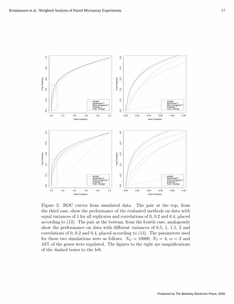
0.0 0.2 0.4 0.6 0.8 1.0

0.0

0.2

0.4

0.6

0.8

1.0

False Positives

Tru

e P

ositi

ves

WAMEModerated TEfron penalized TOrdinary TFold−Change

0.00 0.02 0.04 0.06 0.08 0.10

0.0

0.1

0.2

0.3

0.4

0.5

False PositivesT

rue

Pos

itive

s

WAMEModerated TEfron penalized TOrdinary TFold−Change

0.0 0.2 0.4 0.6 0.8 1.0

0.0

0.2

0.4

0.6

0.8

1.0

False Positives

Tru

e P

ositi

ves

WAMEModerated TEfron penalized TOrdinary TFold−Change

0.00 0.02 0.04 0.06 0.08 0.10

0.0

0.1

0.2

0.3

0.4

0.5

False Positives

Tru

e P

ositi

ves

WAMEModerated TEfron penalized TOrdinary TFold−Change

Figure 2: ROC curves from simulated data. The pair at the top, fromthe third case, show the performance of the evaluated methods on data withequal variances of 1 for all replicates and correlations of 0, 0.2 and 0.4, placedaccording to (13). The pair at the bottom, from the fourth case, analogouslyshow the performance on data with different variances of 0.5, 1, 1.5, 2 andcorrelations of 0, 0.2 and 0.4, placed according to (13). The parameters usedfor these two simulations were as follows. NG = 10000, NI = 4, α = 2 and10% of the genes were regulated. The figures to the right are magnificationsof the dashed boxes to the left.

17Kristiansson et al.: Weighted Analysis of Paired Microarray Experiments

Produced by The Berkeley Electronic Press, 2005

Case Correlation Heavy tails Regulated genes FilterI No No None NoII Yes No None NoIII Yes Yes None NoIV Yes No Yes, 10% NoV Yes No Yes, 10% Yes, 5% removed.

Table 1: Descriptions of the five different settings used in this simulationstudy. When correlations are used, they follow the structure in equation(13).

ward higher variances and α was estimated to be 1.55 instead of 2. Thispattern was also seen when the degrees of freedom were increased to 10 and15 (results not shown). In case IV 10% of the genes were set to be regulatedand since no differentially expressed genes are assumed, the regulation leadsto positive correlations and increased variance estimates. Having 10% of thegenes regulated is a rather high number, but not extreme. Therefore, a filterwas applied to minimise the impact of regulated genes on the estimation ofthe covariance matrix. For each gene g, the filter calculates the minimal ab-solute value of the fold change, which will be denoted Xg,min. Removing thetop 5% of the genes with highest Xg,min gave a much better estimate of Σ,which is included as case V. Note that the genes were only removed from thethe estimate of Σ∗, i.e. the arbitrarily scaled Σ, and not from the estimatesof α and λ. Also note that the number 5% depends on several parameters,such as the total number of regulated genes and the covariance matrix itself.The results of the filtering procedure on real data is presented in the nextsection.

6 Results from real data

WAME was run on three real data sets: the ischemic part of the dataset ofHall et al. (2004), the dataset of Benson et al. (2004) (henceforth referred toas the Cardiac and Polyp datasets, respectively) and the Swirl dataset (de-scribed in Section 3.3 of Dudoit and Yang, 2003). These datasets representmicroarray experiments with different characteristics; different laboratories,both two-colour cDNA and one-channel oligonucleotide (Affymetrix) arrays,different tissues and two different species (human and zebrafish). The Car-diac and Swirl datasets are publicly available.

18 Statistical Applications in Genetics and Molecular Biology Vol. 4 [2005], No. 1, Article 30

http://www.bepress.com/sagmb/vol4/iss1/art30

True Σ Mean estimated Σ Samplestandard deviation

I0.50 0.00 0.00 0.000.00 1.00 0.00 0.000.00 0.00 1.50 0.000.00 0.00 0.00 2.00

0.50 0.00 -0.00 -0.000.00 1.01 -0.00 0.00

-0.00 -0.00 1.51 -0.00-0.00 0.00 -0.00 2.02

0.01 0.01 0.01 0.010.01 0.04 0.02 0.010.02 0.02 0.05 0.020.01 0.01 0.01 0.07

II0.50 0.28 0.17 0.000.40 1.00 0.49 0.280.20 0.40 1.50 0.690.00 0.20 0.40 2.00

0.50 0.28 0.17 0.000.40 1.00 0.50 0.290.20 0.40 1.51 0.700.00 0.20 0.40 2.00

0.02 0.01 0.01 0.010.01 0.04 0.02 0.030.01 0.01 0.06 0.040.01 0.01 0.01 0.11

III0.50 0.28 0.17 0.000.40 1.00 0.49 0.280.20 0.40 1.50 0.690.00 0.20 0.40 2.00

0.51 0.29 0.18 -0.000.40 1.01 0.50 0.280.20 0.40 1.52 0.70

-0.00 0.20 0.40 2.03

0.02 0.01 0.01 0.010.01 0.04 0.02 0.020.01 0.01 0.05 0.030.01 0.01 0.01 0.07

IV0.50 0.28 0.17 0.000.40 1.00 0.49 0.280.20 0.40 1.50 0.690.00 0.20 0.40 2.00

0.61 0.39 0.28 0.110.48 1.11 0.60 0.390.28 0.45 1.61 0.800.10 0.25 0.43 2.11

0.02 0.02 0.02 0.010.01 0.04 0.03 0.010.01 0.01 0.06 0.040.01 0.01 0.01 0.08

V0.50 0.28 0.17 0.000.40 1.00 0.49 0.280.20 0.40 1.50 0.690.00 0.20 0.40 2.00

0.46 0.21 0.11 -0.020.33 0.90 0.38 0.220.14 0.34 1.39 0.59

-0.02 0.16 0.36 1.93

0.01 0.01 0.01 0.020.01 0.02 0.02 0.020.01 0.02 0.06 0.030.02 0.01 0.01 0.07

Table 2: Result from the estimations of Σ from each of the five differentcases. Correlations are shown in italic and covariances in non-italic. Theparameter values used were NG = 10000, NI = 4 and α = 2. The meanvalues and sample standard deviations were calculated from the results of100 simulated datasets. Refer to Table 1 for a description of the differentcases.

19Kristiansson et al.: Weighted Analysis of Paired Microarray Experiments

Produced by The Berkeley Electronic Press, 2005

The Cardiac dataset is described to have been strictly quality controlledby a combination of several available methods. The dataset is thereforeinteresting to examine to see if WAME detects relevant differences in qualityeven in an example of a quality controlled, publicly available dataset. ThePolyp dataset includes one biopsy that was previously thought to be anoutlier and therefore discarded, thus providing a case with one seeminglylesser quality to be detected. In the Swirl dataset, two highly differentiallyexpressed genes exist. Therefore, it is of interest to check that those genes arehighly ranked by WAME. Furthermore, the Swirl dataset has been analysedpreviously in Smyth (2004).

6.1 Cardiac dataset

In the public dataset from Hall et al. (2004), heart biopsies from 19 patientswith heart failure were harvested before and after mechanical support witha ventricular assist device. The aim of the study was to “define criticalregulatory genes governing myocardial remodelling in response to significantreductions in wall stress”, where a first step was to identify differentiallyexpressed genes between the two conditions.

Affymetrix one-channel oligonucleotide arrays of type HG-U133A wereused in the study, each containing 22283 probe-sets. The quality of the ar-rays was controlled using quality measures recommended by Affymetrix aswell as by the program Gene Expressionist (GeneData, Basel, Switzerland).The quality of the different lab steps leading to the actual hybridisationswere controlled using standard methods. The 19 patients were divided intothree groups: ischemic (5 patients), acute myocardial infarction (6 patients)and non-ischemic (8 patients). The ischemic group was the smallest andconsequently the one where quality variations might make the biggest dif-ference. It was therefore chosen for further examination using WAME, tosee if relevant quality variations could be detected despite the close qualitymonitoring.

The dataset was retrieved in raw .CEL-format from the public repositoryGene Expression Omnibus (Edgar et al., 2002). The .CEL-files were subse-quently processed using RMA (Irizarry et al., 2003) on all the arrays of the 19patients simultaneously. Patient-wise log2-ratios of the five ischemic patientswere then formed by taking pairwise differences of the log2 measurementsbefore and after implant.

Applying WAME to the patient-wise log2-ratios provided interesting re-sults. The estimated covariance matrix (see Table 3) suggests that two of thefive patients (I13 and I7) were substantially more variable than the others,

20 Statistical Applications in Genetics and Molecular Biology Vol. 4 [2005], No. 1, Article 30

http://www.bepress.com/sagmb/vol4/iss1/art30

while the correlations between patients were rather limited. These numbersseem credible when examining Figure 3, where for each pair of patients, therespective log2-ratios of all genes were plotted against each other. The plotsclearly show that the observations of the two patients in question (I13 andI7) are more variable than the others.

The corresponding weights, derived from the estimated covariance matrixΣ, are shown in Table 4. As was discussed in Sections 4.1 and 5.2, whenestimating Σ all genes are assumed to be non-differentially expressed. Toexamine the impact of potentially regulated genes on the estimation of Σ,the analysis was redone, removing genes with high lowest absolute log2-ratioin the estimation of Σ, as described in Section 5.2. The individual elementsof the estimated covariance matrix and of α changed only slightly, even whenas much as 50% of the data was removed (data not shown). This is reflectedin the weights in Table 4.

PatientPatient I12 I13 I4 I7 I8

I12 0.046 0.003 0.001 0.012 0.002I13 0.033 0.196 -0.014 0.007 -0.001I4 0.023 -0.126 0.065 0.013 0.002I7 0.111 0.030 0.102 0.258 -0.017I8 0.040 -0.011 0.038 -0.152 0.047

Table 3: Estimated covariance-correlation matrix, Σ, for patients in the Car-diac dataset. (Correlations in italic, covariances in non-italic.)

PatientRemoved genes I12 I13 I4 I7 I8

none 0.297 0.091 0.232 0.053 0.3265% 0.301 0.089 0.233 0.054 0.32310% 0.303 0.087 0.235 0.053 0.32150% 0.323 0.082 0.240 0.046 0.308

Table 4: Weights for patients in the Cardiac dataset. Different numbers ofpotentially regulated genes were removed in the estimation of Σ, to checktheir influence. Potential regulation was measured by minimal absolute log2-ratio among the patients.

The hyperparameter α related to the spread of the gene-specific variance

21Kristiansson et al.: Weighted Analysis of Paired Microarray Experiments

Produced by The Berkeley Electronic Press, 2005

Figure 3: Pair-wise plots of the log2-ratios of the patients in the Cardiacdataset. The plots to the lower-left show two-dimensional kernel densityestimates of the distribution of log2-ratios in each pair of patients. This pro-vides information in the central areas where the corresponding scatterplotsare solid black (cf. Figure 6 in Huber et al., 2003). The colour-scale is, inincreasing level of density: white, grey, black and red.

22 Statistical Applications in Genetics and Molecular Biology Vol. 4 [2005], No. 1, Article 30

http://www.bepress.com/sagmb/vol4/iss1/art30

scaling factors, cg, was estimated to be 1.92, giving a heavy tail for theprior distribution. Thus removing cg by transformation when estimating Σ(Section 4.1) is justified.

Inspecting the fitted distribution of Sg given α = 1.92 against the em-pirical distribution of Sg reveals a good fit (see Figure 4), implying that thefamily of inverse gamma prior distributions is rich enough for this dataset.

Den

sity

0 5 10 15 20 25

0.00

0.10

0.20

0.30

empiricalfitted

Figure 4: Empirical distribution of Sg in the Cardiac dataset, together withthe density of Sg given α = 1.92.

Examining the observed values of the statistic, Tg, compared to the ex-pected null distribution reveals a good overall concordance (see Figure 5).Some genes have a larger tg than can be explained by the null distribution,which points toward some of them being up-regulated by the treatment (seethe qq-plot in Figure 5).

6.2 Polyp dataset

In the dataset from Benson et al. (2004), biopsies from nasal polyps of fivepatients were taken before and after treatment with local glucocorticoids.The goal was to examine closer the mechanisms behind the effect of thetreatment and one step was to identify differentially expressed genes. Tech-nical duplicates stemming from the same extracted RNA were run for eachbiopsy on Affymetrix HG-U133A arrays. This gave a dataset of 20 arraysand 22283 probe-sets.

Comparing each of the arrays in the dataset with all arrays from otherpatients and/or conditions, by looking at pair-wise scatterplots, the arraysfrom before treatment of patient 2 consistently showed larger variation thanany other. The biopsy in question was found to be considerably smaller thanthe others, providing possible explanations such as non-representativeness

23Kristiansson et al.: Weighted Analysis of Paired Microarray Experiments

Produced by The Berkeley Electronic Press, 2005

Den

sity

−5 0 5 10

0.0

0.1

0.2

0.3

0.4

−5 0 5

−5

05

10

Obs

erve

d T

g

Figure 5: To the left, a histogram of the observed Tg-values together with thedensity of the null distribution (in red), in the Cardiac dataset. To the right, aquantile-quantile plot where the observed values of Tg are plotted against thequantiles of Tg under the null hypothesis. The central part of the empiricaldistribution follows the identity line well, showing good concordance withthe null distribution. For high positive Tg-values, the observations clearlydeviate from the predicted ones, pointing at the existence of up-regulatedgenes.

in tissue distribution. The data from patient 2 was therefore excluded inBenson et al. (2004).

WAME would preferably identify the patient 2 observation as havinglarger variation and downweight it. The data was processed using RMA(Irizarry et al., 2003) and the log2-ratio for each patient was formed by takingdifferences between the averages over the technical duplicates, before andafter treatment, combining 4 arrays for each patient into one set of log2-ratios. Making one scatter plot of the two sets of log2-ratios for each pairof patients (Figure 6) clearly indicates that patient 2 is more variable thanpatients 1,3 and 5. Interestingly, the measurements from patients 1 and 2seem to be highly correlated and patient 4 seems to have high variability.

Estimating the covariance matrix, Σ, the correlation between patients 1and 2 is estimated to 0.82 (see Table 5), which is high but not unbelievablewhen studying Figure 6. The variance of patient 2 is furthermore estimatedto be four times that of patient 1. Examining the resulting weights, patient 2actually receives a weight of −2% (see Table 6). The negativeness is a resultof its variance being much higher than that of patient 1, together with thembeing highly correlated. As negative weights seem questionable, a natural

24 Statistical Applications in Genetics and Molecular Biology Vol. 4 [2005], No. 1, Article 30

http://www.bepress.com/sagmb/vol4/iss1/art30

Figure 6: Pair-wise plots of the log2-ratios of the patients in the Polypdataset. The plots to the lower-left show two-dimensional kernel densityestimates of the distribution of log2-ratios in each pair of patients. This pro-vides information in the central areas where the corresponding scatterplotsare solid black (cf. Figure 6 in Huber et al., 2003). The colour-scale is, inincreasing level of density: white, grey, black and red.

25Kristiansson et al.: Weighted Analysis of Paired Microarray Experiments

Produced by The Berkeley Electronic Press, 2005

solution is to remove patient 2, which was done in (Benson et al., 2004).Beside the result of the very low weight for patient 2, the other patientsreceive distinctly different weights, which is interesting.

PatientPatient 1 2 3 4 5

1 0.300 0.493 0.000 -0.012 -0.0672 0.822 1.200 0.004 0.041 -0.1573 0.002 0.012 0.091 -0.071 -0.0554 -0.038 0.067 -0.417 0.319 0.1025 -0.291 -0.340 -0.434 0.430 0.178

Table 5: Estimated covariance-correlation matrix, Σ, for patients in thePolyp dataset. (Correlations in italic, covariances in non-italic.)

PatientRemoved genes 1 2 3 4 5

none 0.179 -0.026 0.483 0.104 0.2605% 0.181 -0.025 0.481 0.104 0.25910% 0.180 -0.024 0.482 0.103 0.25950% 0.157 -0.015 0.506 0.100 0.252

Table 6: Weights for the patients in the Polyp dataset. Different numbers ofpotentially regulated genes were removed, to check their potential influence inthe estimation of Σ. Potential regulation was measured by minimal absolutelog2-ratio among the patients.

The hyperparameter α, related to the spread of the gene-specific variancescaling factors, cg, was estimated to 1.97, giving infinite variance for thedistribution of cg. The fit of Sg given α = 1.97 was very good (see Figure 10in the Appendix).

As in the Cardiac dataset, the weights were steadily estimated whenpotentially regulated genes were removed in the estimation of the covariancematrix Σ (see Table 6). The estimated correlations between patients 3, 4and 5 were reduced somewhat. Removing 5% of the genes reduced thosecorrelations by 0.03-0.04 and removing 10% reduced them by 0.06-0.07. Thehigh correlation between patient 1 and 2 was only slightly reduced (<0.03),even when 50% of the genes were removed.

26 Statistical Applications in Genetics and Molecular Biology Vol. 4 [2005], No. 1, Article 30

http://www.bepress.com/sagmb/vol4/iss1/art30

Examining the observed values of the statistic, Tg, compared to the ex-pected null distribution (see Figure 7) reveals a good overall concordance.Some genes have a more extreme Tg than can be explained by the null distri-bution, which points toward many of them being regulated by the treatment(see the qq-plot in Figure 7).

Den

sity

−5 0 5

0.0

0.1

0.2

0.3

0.4

−5 0 5

−5

05

Obs

erve

d T

g

Figure 7: To the left, a histogram of the observed Tg-values together with thedensity of the null distribution (in red), in the Polyp dataset. To the right, aquantile-quantile plot where the observed values of Tg are plotted against thequantiles of Tg under the null hypothesis. The central part of the empiricaldistribution follows the identity line well, showing good concordance withthe null distribution. For extreme Tg-values, the observations clearly deviatefrom the predicted ones, pointing at the existence of regulated genes.

6.3 Swirl dataset

In the Swirl experiment (Dudoit and Yang, 2003), one goal was to identifygenes that are differentially expressed in zebrafish carrying a point mutatedSRB2 gene, compared to ordinary, wild-type zebrafish. SRB2 and one of itsknown targets, Dlx3 are expected to be highly differentially expressed in thisexperiment, thus these genes should be highly ranked using WAME. TheSwirl dataset has been examined in Smyth (2004).

The dataset consists of four two-colour cDNA microarrays with 8448spots, with publicly available data. We used standard pre-processing tocompensate for effects such as background and dye bias. Background cor-rection subtract and within-array normalisation print tip loess were used in

27Kristiansson et al.: Weighted Analysis of Paired Microarray Experiments

Produced by The Berkeley Electronic Press, 2005

the LIMMA package (Smyth et al., 2003). Between-array scale normalisation(Yang et al., 2002) was not performed in contrast to the analysis in Smyth(2004). When including between-array scale normalisation in combinationwith LIMMA in the simulation study of Section 5.1 the performance was notnotably increased (results not shown). However, the model used for simu-lation leaves the signals unaffected when noise levels varies, which may bequestionable for some sources of variation.

Making one scatter plot of the log2-ratios for each pair of arrays (Figure 8)indicates that array 2 is less variable than the others, while the genes withlowest log2-ratio on array 1 seem to be outliers, since they are not extreme inany other array. Examining the estimated covariance matrix (see Table 7),array 2 indeed receives the highest variance. In addition, there are substantialcorrelations between arrays 1 and 3, 2 and 4 and 3 and 4, which is alsoindicated by the scatter-plots (Figure 8).

ArrayArray 1 2 3 4

1 0.128 0.007 0.079 0.0172 0.066 0.086 -0.002 0.0383 0.489 -0.017 0.203 0.0764 0.136 0.371 0.482 0.124

Table 7: Estimated covariance-correlation matrix, Σ, for the arrays in theSwirl dataset. (Correlations in italic, covariances in non-italic.)

When re-performing the estimation of Σ after removing potentially regu-lated genes (in analogy with the analyses of the Polyp and Cardiac datasets),the correlations were decreased somewhat. Removing 5% of the genes de-creased the three high correlations by 0.02-0.06, while removing 10% de-creased them by 0.04-0.08. However, the corresponding weights only changedmarginally (see Table 8).

The hyperparameter α was estimated to 1.89. Further analysis of thedataset shows that the distribution of Sg fits the predicted distribution of Sg

well given α = 1.89 (see Figure 11 in in the Appendix). The observed valuesof the statistic, Tg, seem to fit the null distribution well (see Figure 9).

Since the point mutated gene, SRB2 and one of its known targets, Dlx3,are expected to be highly differentially expressed, their actual ranking is ofinterest. In Table 9 below, the top 20 genes as ranked by WAME are listed.The values of some widely used statistics are included for comparison. Therankings by WAME and the moderated t-statistic (Smyth et al., 2003) are

28 Statistical Applications in Genetics and Molecular Biology Vol. 4 [2005], No. 1, Article 30

http://www.bepress.com/sagmb/vol4/iss1/art30

Figure 8: Pair-wise plots of the log2-ratios of the arrays in the Swirl dataset.The plots to the lower-left show two-dimensional kernel density estimates ofthe distribution of log2-ratios in each pair of patients. This provides infor-mation in the central areas where the corresponding scatterplots are solidblack (cf. Figure 6 in Huber et al., 2003). The colour-scale is, in increasinglevel of density: white, grey, black and red.

29Kristiansson et al.: Weighted Analysis of Paired Microarray Experiments

Produced by The Berkeley Electronic Press, 2005

ArrayRemoved genes 1 2 3 4

none 0.289 0.474 0.072 0.1655% 0.288 0.469 0.076 0.16610% 0.290 0.462 0.075 0.17350% 0.282 0.447 0.087 0.184

Table 8: Weights for the arrays in the Swirl dataset. Different numbers ofpotentially regulated genes were removed, to check their potential influence inthe estimation of Σ. Potential regulation was measured by minimal absolutelog2-ratio among the arrays.

Den

sity

−15 −10 −5 0 5 10

0.0

0.1

0.2

0.3

0.4

−5 0 5

−15

−10

−5

05

10

Obs

erve

d T

g

Figure 9: To the left, a histogram of the observed Tg-values together with thedensity of the null distribution (in red), in the Swirl dataset. To the right, aquantile-quantile plot where the observed values of Tg are plotted against thequantiles of Tg under the null hypothesis. The central part of the empiricaldistribution follows the identity line well, showing good concordance withthe null distribution. For extreme Tg-values, the observations clearly deviatefrom the predicted ones, pointing at the existence of regulated genes.

30 Statistical Applications in Genetics and Molecular Biology Vol. 4 [2005], No. 1, Article 30

http://www.bepress.com/sagmb/vol4/iss1/art30

quite similar, while the rankings by the ordinary t-statistic and the averagelog2-ratio (i.e. fold change) are rather different than the one by WAME,which was expected. All four spots for the two validated genes are includedin WAME’s top 20 list (see Table 9). It could be noted that the ordinary t-statistics and LIMMA’s moderated t-statistics are both generally numericallylarger than the WAME values. One reason for this seems to be that thereference distributions of the ordinary t-statistics and LIMMA’s moderatedt-statistics show q-q plots that differ from the reference distribution by ahigher slope also in the central part (data not shown but compare the figureon page 24 in Smyth et al. (2003)) in contrast to the plot in the right partof Figure 9. We have also performed a simulation study with a covariancematrix as in Table 7 and with 10% of the genes differentially expressed. Itshows better ROC curves with WAME than with the other two methods(data not shown) in a similar way as in Figure 2.

7 Discussion

A problem with the microarray technology is that it involves several consec-utive steps, each exhibiting large quality variations. Thus there is a strongneed for quality assessment and quality control to handle occurrences ofpoor quality. In this paper, we introduce the WAME method for the anal-ysis of paired microarray experiments, which aims at estimating array- orrepetition-wide quality deviations and integrates these estimates in the sta-tistical analysis.

The quality deviations are modelled here as different variances for differ-ent repetitions (e.g. arrays) as well as correlations between them in a covari-ance matrix Σ, catching both unequal precision and systematic errors. Geneshave different variability (biological and technical), which is modelled by agene-specific variance scaling factor cg. Given this structure, the pair-wisemeasured log2-ratios for each gene are assumed to be normally distributed.

Estimation of the covariance matrix is complicated by the gene-specificscaling factors and unknown differential expressions µg. We assume thatmost genes are not differentially expressed (µg = 0) and the gene-specificscaling factors are removed by a transformation. A scaled version of Σ isestimated by numerical maximum likelihood. The assumed restricted dif-ferential expression restrains the experimental setups that can be analysed,but similar assumptions are made in procedures that have become de factostandard in the (preceding) normalisation step.

Since most microarray experiments contain only a few repetitions, the

31Kristiansson et al.: Weighted Analysis of Paired Microarray Experiments

Produced by The Berkeley Electronic Press, 2005

Name ID average ordinary moderated WAMElog2-ratio t-statistic t-statistic

fb85d05 18-F10 -2.66 -18.41 -20.79 -15.15fb58g10 11-L19 -1.60 -14.32 -14.15 -11.51control Dlx3 -2.19 -15.91 -17.57 -11.17control Dlx3 -2.19 -13.58 -16.08 -9.84

fb24g06 3-D11 1.32 19.52 13.62 9.80fb54e03 10-K5 -1.20 -25.74 -13.11 -9.66fc22a09 27-E17 1.26 24.76 13.68 9.50fb40h07 7-D14 1.35 14.15 12.69 9.12fb85a01 18-E1 -1.29 -17.35 -13.01 -8.81fb87f03 18-O6 -1.08 -27.90 -12.06 -8.80fb37e11 6-G21 1.23 14.37 11.94 8.47fb94h06 20-L12 1.28 15.41 12.54 8.46fb87d12 18-N24 1.28 12.96 11.87 8.39control BMP2 -2.24 -8.63 -11.78 -8.33fc10h09 24-H18 1.20 15.05 11.92 8.23fb85f09 18-G18 1.29 11.50 11.38 8.22control BMP2 -2.33 -8.37 -11.58 -7.95

fb26b10 3-I20 1.09 15.50 11.17 7.81fb37b09 6-E18 1.31 11.57 11.55 7.78fc22f05 27-G10 -1.19 -10.42 -10.44 -7.70

Table 9: The top 20 most probably regulated genes in the Swirl datasetaccording to WAME.

32 Statistical Applications in Genetics and Molecular Biology Vol. 4 [2005], No. 1, Article 30

http://www.bepress.com/sagmb/vol4/iss1/art30

estimates of the gene-specific variance scaling factors cg are imprecise, whichmay lead to false conclusions. An empirical Bayes approach is used with aninverse gamma prior distribution that moderates extreme estimates similarto (Baldi and Long, 2001; Lonnstedt and Speed, 2002; Smyth, 2004). The hy-perparameter α determining the spread of the prior distribution is estimatedby numerical maximum likelihood together with the scale of the previouslyestimated arbitrarily scaled Σ.

In the present paper, quality is modelled in a general manner by thecovariance structure matrix Σ. In some microarray experiments, additionalinformation is available, for example, shared sources of variation may beknown. Quantitative quality measures may also be available, e.g. spot shapefeatures or residuals from the fitting of probe-level models (Bolstad, 2004).It is possible to explicitly model some such sources of variation, for exampleusing random or fixed effects (cf. Bakewell and Wit (2005)) and to includequality measures as covariates. However, such models would likely focus onsome of the clearer sources of variation but leave out more involved and hardmodelled sources. One can view our method as an attempt to identify theeffects on the single gene level of those variability sources, with the priordistribution modelling the noise structure of a random gene from the wholegene population. An approach combining explicit modelling with a generalcovariance structure would be interesting as future work.

To identify differentially expressed genes a likelihood-ratio test is derived,resulting in the weighted moderated t-statistic, which is a generalisation ofthe moderated t-statistic in Smyth (2004). The estimated covariance matrixΣ is used to produce both weights for the different repetitions and gene-specific variance estimates. The weighted mean is the estimate of differentialexpression with minimal variance.

As discussed above, array- or repetition-wide quality deviations in allsteps leading to the observed log2-ratios are estimated and incorporated inthe analysis. The current paper is restricted to paired two-sample settingswhere most genes are non-differentially expressed. A generalisation similarto Smyth (2004) should be possible for experiments with pairwise measure-ments. The scaled estimate of the covariance matrix Σ could be calculatedaccording to the procedure in the current paper (cf. Section 4.1). The un-known scale of the covariance estimate, as well as the parameter α of theprior distribution for the gene-specific variance scales, could be estimatedutilising generalised residual sums of squares for all genes, appropriately de-fined through the norm determined by Σ (cf. Sg in Section 4.2). Tests forsingle or multiple identifiable linear combinations of expected values couldbe derived as in the current paper to get weighted moderated t-statistics and

33Kristiansson et al.: Weighted Analysis of Paired Microarray Experiments

Produced by The Berkeley Electronic Press, 2005

modified F -statistics. Work on generalisations, with simulated and real datasets is in progress.

A simulation study was done to compare the performance of WAMEto four published methods. On data without correlations and with equalvariances between repetitions, WAME performs as well as the moderatedt-statistic which assumes this structure. When correlations and/or unequalvariances are included, WAME performs better than the other methods. Inone case, using WAME results in almost a third less false positives whichcan correspond to hundreds of genes. Evaluating the point estimator of thecovariance matrix Σ revealed good precision and accuracy when no regulatedgenes were present. Including 10% regulated genes resulted in a bias, whichwas partly handled by removing genes likely to be regulated. In both casesestimation of the hyperparameter α was nearly unbiased and accurate. Theestimate of Σ was essentially unbiased when heavy tails were introduced incontrast to the estimate of α which was 1.55 instead of 2. As a practical con-sideration, filtering of seemingly regulated genes may be appropriate whena relatively large number of genes can be expected to be regulated. How-ever, results from real and simulated data indicate that such filtering resultsin largely unchanged weights, reducing its importance. Also, in the casesstudied the unfiltered statistic is slightly conservative (results not shown).

Three real datasets were analysed: the ischemic part of the dataset ofHall et al. (2004), the dataset of Benson et al. (2004) and the Swirl dataset(Dudoit and Yang, 2003). In all cases, relevant correlations and differences inprecision between replicates were found, even in the first dataset which hadbeen quality controlled using several available methods. The exact originof the correlations is an interesting, open question. In the second datasetone previously identified outlier was practically removed by WAME. In theSwirl dataset, expected differentially expressed genes are ranked among thetop 20. Relevant empirical distributions showed good fit to the theoreticaldistributions, indicating that the family of prior distributions for cg is flexibleenough and that the normality assumption is satisfactory.

The model used in WAME is optimistic in several ways. Exact normalityis not to be expected and the independence between the genes is hard tofully justify. The noise structure may also be different for the regulatedgenes, e.g. if there are several normalising procedures involved in the pre-processing step. This may affect the power, which points towards the use ofa moderated impact of Σ on the weights in the final analysis. Thus, evenif simulations under the model assumptions show highly promising results,there are many experimental situations where the model assumptions maynot be justified. We intend to look further into different robustness questions

34 Statistical Applications in Genetics and Molecular Biology Vol. 4 [2005], No. 1, Article 30

http://www.bepress.com/sagmb/vol4/iss1/art30

for model deviations in the future.The role of microarray experiments is often to test for regulation of tens

of thousands of genes as an exploratory tool to derive candidate rankinglists of potentially regulated genes, which in subsequent steps will be biologi-cally interpreted and validated by more precise techniques. We find that ourapproach competes well with other methods in the production of such lists.

To summarise, WAME estimates and integrates array- or repetition-widequality deviations in the analysis of paired microarray experiments. An em-pirical Bayes approach is used to moderate the gene-specific variance esti-mates, resulting in a weighted moderated t-statistic with a derived distribu-tion. The performance of WAME has been evaluated on both simulated andreal microarray data. The simulations show a considerable advantage relativeto four other methods studied, particularly for data with unequal variancesor correlations among repetitions. The three real datasets studied indicatethat data with unequal variances or correlations should be quite common.The model controls with diagnostic plots also show satisfactory results forall three real datasets.

35Kristiansson et al.: Weighted Analysis of Paired Microarray Experiments

Produced by The Berkeley Electronic Press, 2005

Appendix

Additional Figures

Den

sity

0 5 10 15 20 25

0.00

0.10

0.20

0.30

empiricalfitted

Figure 10: Empirical distribution of Sg in the Polyp dataset, together withthe density of Sg given α = 1.97.

Den

sity

0 5 10 15 20 25

0.0

0.2

0.4 empirical

fitted

Figure 11: Empirical distribution of Sg in the Swirl dataset, together withthe density of Sg given α = 1.89.

36 Statistical Applications in Genetics and Molecular Biology Vol. 4 [2005], No. 1, Article 30

http://www.bepress.com/sagmb/vol4/iss1/art30

Mathematical details

We observe Xg = (Xg1, . . . , XgNI) where g = 1, . . . , NG. Let Σ be a covari-

ance structure matrix for the NI repetitions, cg a set of gene-specific variancescaling factors and α a hyperparameter determining the shape of the priordistribution for cg. Then for fixed µg, Σ and α,

cg ∼ Γ−1(α, 1),

Xg | cg ∼ NNI(µg1, cgΣ)

and all variables corresponding to different genes are assumed independent.

Estimation of a scaled version of the matrix Σ

Assume that µg = 0 for all g. Under this assumption, it is possible to derivea scale independent estimate of the covariance matrix Σ by a transformationof the vector Xg. This is done as follows (the index g is dropped to increasethe readability). Let U = (U1, . . . , UNI

) where

Ui =

{X1 if i = 1Xi/X1 if 2 ≤ i ≤ NI .

The inverse becomes

Xi =

{U1 if i = 1UiU1 if 2 ≤ i ≤ NI

and the Jacobian can be derived to

J(u1, . . . , uNI) = uNI−1

1 ,

so for U ∈ RNI the density becomes

fU | c,Σ(u) = fX | c,Σ (x(u)) |J(u)|

= (2π)−NI/2 c−NI/2 |Σ|−1/2 |u1|NI−1e−u21

2cvTΣ−1v.

where v = (1, u2, . . . , uNI)T. Integration over u1 yields

fU2,...,UNI| Σ(u2, . . . , uNI

| Σ) =

∫ ∞

−∞fU | c,Σ(u | c, Σ) du1

= C |Σ|−1/2 [vTΣ−1v

]−NI/2,

(14)

37Kristiansson et al.: Weighted Analysis of Paired Microarray Experiments

Produced by The Berkeley Electronic Press, 2005

where C is a normalisation constant and v is defined as above. This densityis scale invariant with respect to the parameter Σ in the sense that for anyscalar λ,

fU2,...,UNI| Σ(u2, . . . , uNI

|λΣ) = fU2,...,UNI| Σ(u2, . . . , uNI

|Σ).

Thus, it is also independent of c and under the assumption of independentgenes, the log-likelihood function becomes

l(Σ) = C ′ − NG

2log (|Σ|)− NI

2

Ng∑g=1

log(vT

gΣ−1vg

),

where C ′ is a constant that is independent of Σ. Numerical maximisationyields a scaled version of Σ, denoted Σ∗. Here the first element in the firstrow of Σ∗ is fixed to one.

Estimation of the hyperparameter α and the scale λ

From the model assumptions, we know that

cg ∼ Γ−1(α, 1).

Assume that Σ is known and define

Sg = (AXg)T(AΣAT)−1AXg,

where A is a contrast matrix, i.e. a matrix of dimension NI − 1 × NI , withfull rank and with each row sum equal to 0. It follows that

Sg ∼ cg × χ2NI−1 .

The unconditional distribution of Sg can be derived by integrating over cg,i.e.,

fSg | α(sg) =

∫ ∞

0

fSg | cg(s)fcg | α(cg) dcg

=1

2

(s/2)(NI−1)/2−1

Γ (α) Γ((NI − 1)/2)

∫ ∞

0

c−α−(NI−1)/2−1e−(s/2+1)/cg dcg

=1

2

Γ(α + (NI − 1)/2)

Γ(α)Γ((NI − 1)/2)

(s/2)(NI−1)/2−1

[1 + s/2]α+(NI−1)/2.

This is a beta prime distribution (also called a beta distribution of the secondkind) (Johnson et al., 1995) with parameters NI − 1 and α which is denoted

38 Statistical Applications in Genetics and Molecular Biology Vol. 4 [2005], No. 1, Article 30

http://www.bepress.com/sagmb/vol4/iss1/art30

β′(NI−1, α). Since only a scaled version of Σ, denoted Σ∗, is assumed knownfrom the primary estimation step, the following entities are defined. Let

Σ∗ = λΣ

S∗g = (AXg)

T(AΣ∗AT)−1AXG = Sg/λ,

where λ is the unknown scale for Σ∗. It follows that

S∗g ∼ 2/λ× β′(NI − 1, α).

The log likelihood function for S∗g can be derived to

l(α, λ|{sg}NGg=1) = C + NG [(NI − 1)/2 log(λ) + log Γ(α + (NI − 1)/2)− log Γ(α)]

− (α + (NI − 1)/2)

NG∑g=1

log(sgλ/2 + 1).

Numerical maximum likelihood is used to estimate α and λ, which togetherwith Σ∗ can be used to calculate an estimate for Σ.

Inference about µg

The hypotheses that are interesting to test are if different genes are regulatedor not, that is for each g,

H0 : gene g is not regulated (µg = 0)

HA : gene g is regulated (µg 6= 0).

To test these hypotheses a maximum likelihood ratio (LRT) test is derived.For each g, we reject H0 if

supµg 6=0

L (µg|xg)

L (0|xg)≥ k,

where 1 ≤ k < ∞. The likelihood L can be calculated by integration overcg, i.e.

L (µg|x) =

∫fX | µg ,cg ,Σ(x)fcg | α(cg) dcg

= (2π)−NI/2 |Σ|−1/2 Γ(NI/2 + α)

Γ(α)

[(xg − µg1)T Σ−1 (xg − µg1)

2+ 1

]−NI/2−α

.

39Kristiansson et al.: Weighted Analysis of Paired Microarray Experiments

Produced by The Berkeley Electronic Press, 2005

To calculate the numerator in the likelihood ratio we need to maximise Lover µg, which is the same as minimising

(xg − µg1)T Σ−1 (xg − µg1) .

A little algebra shows that this optimum corresponds to the argument

µg =1TΣ−1

1TΣ−11xg .

We will use xwg to denote this weighted sum and it can be shown to be

the weighted mean with least variance. The maximum value of the likelihoodfunction becomes

L(xwg |xg) = (2π)−NI/2 |Σ|−1/2 Γ(NI/2 + α)

Γ(α)

[xT

gΣ−1xg − (xw

g )21TΣ−11

2+ 1

].

Using this, the likelihood ratio test statistic can be rewritten as

L(xw

g |xg

)L (0|xg)

=

[xT

gΣ−1xg + 2

xTgΣ

−1xg −(xw

g

)21TΣ−11 + 2

]NI/2+α

=

[1 +

(xw

g

)21TΣ−11

xgΣ−1xg −(xw

g

)21TΣ−11 + 2

]NI/2+α

=

[1 +

(xw

g

)21TΣ−11(

xg −(xw

g

)1)T

Σ−1(xg −

(xw

g

)1)

+ 2

]NI/2+α

=

[1 +

(xwg )21TΣ−11

(Awxg)T Σ−1 (Awxg) + 2

]NI/2+α

where Aw is the contrast matrix

Aw =

1− w1 −w2 −w3 . . . −wNI

−w1 1− w2 −w3 . . . −wNI

. . . . . . . . . . . . . . .−w1 −w2 −w3 . . . 1− wNI

and wi is the i:th element of the vector

1TΣ−1

1TΣ−11.

40 Statistical Applications in Genetics and Molecular Biology Vol. 4 [2005], No. 1, Article 30

http://www.bepress.com/sagmb/vol4/iss1/art30

The next step is to show that

(Awxg)T Σ−1 (Awxg) = sg . (15)

To do that, we first note that for any pair of contrast matrices A1 and A2

with NI columns and of rank NI − 1, with each row sum equal to zero,

(A1xg)T (A1ΣAT

1)− (A1xg) = (A2xg)

T (A2ΣAT

2)− (A2xg) .

Here a generalised inverse is used, defined as BB−B = B, which gives

B−1 = B−

when B is invertible. Now,

sg = (Axg)T (AΣAT)−1 (Axg) = (Awxg)

T (AwΣAT

w)− (Awxg) ,

so we can prove (15) by showing that

(Awxg)T Σ−1 (Awxg) = (Awxg)

T (AwΣAT

w)− (Awxg) .

Since Aw is idempotent, this is the same as proving that

(AwΣAwT)− = AT

wΣ−1Aw .

Writing Aw as

Aw = I − 11TΣ−1

1TΣ−11

it follows that

AwΣAT

w

(AT

wΣ−1Aw

)AwΣAT

w =AwΣAT

wΣ−1AwΣAT

w

=

[I − 1

1TΣ−1

1TΣ−11

]Σ

[I − 1

1TΣ−1

1TΣ−11

]T

Σ−1

×[I − 1

1TΣ−1

1TΣ−11

]Σ

[I − 1

1TΣ−1

1TΣ−11

]T

=

[Σ− 11T

1TΣ−11

]Σ−1

[Σ− 11T

1TΣ−11

]=Σ− 11T

1TΣ−11= AwΣAT

w .

Thus,(AwΣAT

w)− = AT

wΣ−1Aw

41Kristiansson et al.: Weighted Analysis of Paired Microarray Experiments

Produced by The Berkeley Electronic Press, 2005

and (15) is proved.Using this result, we can write the LRT as

|xwg |√

sg + 2≥ k′, (16)

where 0 ≤ k′ < ∞ is a new constant. To derive the distribution of thestatistic that corresponds to (16) under the null hypothesis, we proceed asfollows. Let

Tg =√

1TΣ−11 (NI − 1 + 2α)Xw

g√Sg + 2

.

Then sinceXw

g ∼ N(0,

cg

1TΣ−11

)it can be shown that Xw

g is independent to all elements of AwXg and thusto Sg. Furthermore,

Tg =Xw

g /√

cg/1TΣ−11√Sg/cg + 2/cg/

√NI − 1 + 2α

,

where the numerator is independent of Sg and has the same normal distri-bution conditionally on all cg (and thus also unconditionally), showing thatthe denominator in this ratio expression is independent of the numerator. Asimilar argument shows that Sg/cg and 2/cg are independent, and since theyare chi-square distributed with NI−1 and 2α degrees of freedom respectively,the sum is chi-square distributed with NI−1+2α degrees of freedom. Hence,under the null hypothesis, Tg is a t-distribution with NI − 1 + 2α degrees offreedom,

Tg | Σ, α ∼ tNI−1+2α .

We call Tg the weighted moderated t-statistic.

References

D.J. Bakewell and E. Wit. Weighted analysis of microarray gene expressionusing maximum-likelihood. Bioinformatics, 21(6):723–729, 2005.

P. Baldi and A.D. Long. A Bayesian framework for the analysis of microar-ray expression data: regularized t-test and statistical inferences of genechanges. Bioinformatics, 17(6):509–519, 2001.

42 Statistical Applications in Genetics and Molecular Biology Vol. 4 [2005], No. 1, Article 30

http://www.bepress.com/sagmb/vol4/iss1/art30

M. Benson, L. Carlsson, M. Adner, M. Jernas, M. Rudemo, A. Sjogren,P.A. Svensson, R. Uddman, and Cardell L.O. Gene profiling reveals in-creased expression of uteroglobin and other anti-inflammatory genes inglucocorticoid-treated nasal polyps. Journal of Allergy and Clinical Im-munology, 113(6):1137–1143, 2004.

B.M. Bolstad. Low-level Analysis of High-density Oligonucleotide ArrayData: Background, Normalization and Summarization. PhD thesis, Uni-versity of California, Berkeley, California, 2004.

D.-T. Chen. A graphical approach for quality control of oligonucleotide arraydata. Journal of Biopharmaceutical Statistics, 14(3):591–606, 2004.

S. Dudoit and J.Y.H. Yang. Bioconductor R packages for exploratory dataanalysis and normalization of cDNA microarray data. In G. Parmigiani,E.S. Garett, R.A. Irizarry, and S.L. Zeger, editors, The Analysis of GeneExpression Data. Springer, 2003.

C.I. Dumur, S. Nasim, A.M. Best, K.J. Archer, A.C. Ladd, V.R. Mas, D.S.Wilkinson, C.T. Garret, and A. Ferreira-Gonzalez. Evaluation of quality-control criteria for microarray gene expression analysis. Clinical Chemistry,50(11):1994–2002, 2004.

R. Edgar, M. Domrachev, and A.E. Lash. Gene Expression Omnibus: NCBIgene expression and hybridization array data repository. Nucleic AcidsResearch, 30(1):207–210, 2002.

B. Efron, R. Tibshirani, J.D. Storey, and V. Tusher. Empirical Bayes analysisof a microarray experiment. Journal of the American Statistical Associa-tion, 96(456):1151–1160, 2001.

J.L. Hall, S. Grindle, X. Han, D. Fermin, S. Park, Y. Chen, R.J. Bache,A. Mariash, Z. Guan, S. Ormaza, J. Thompson, J. Graziano, S.E.de Sam Lazaro, S. Pan, R.D. Simari, and L.W. Miller. Genomic pro-filing of the human heart before and after mechanical support witha ventricular assist device reveals alterations in vascular signaling net-works. Journal of Physiological Genomics, 17(3):283–291, 2004. URLhttp://www.ncbi.nlm.nih.gov/geo/query/acc.cgi?acc=GDS558.

S. Hautaniemi, H. Edgren, P. Vesanen, M. Wolf, A.-K. Jarvinen, O. Yli-Harja, J. Astola, K. Olli, and O. Monni. A novel strategy for microarrayquality control using bayesian networks. Bioinformatics, 19(16):2031–2038,2003.

43Kristiansson et al.: Weighted Analysis of Paired Microarray Experiments

Produced by The Berkeley Electronic Press, 2005

W. Huber, A. von Heydebreck, and M. Vingron. Analysis of microarraygene expression data. In M. et al. Bishop, editor, Handbook of StatisticalGenetics, 2nd Edition. John Wiley & Sons, 2003.

R.A. Irizarry, B.M. Bolstad, F. Collin, L.M. Cope, B. Hobbs, and T.P. Speed.Summaries of Affymetrix GeneChip probe level data. Nucleic Acids Re-search, 31(4):e15, 2003.

K. Johnson and S. Lin. QA/QC as a pressing need for microarray analysis:meeting report from CAMDA’02. BioTechniques, 34(suppl):S62–S63, 32003.

N.L. Johnson, S. Kotz, and N. Balakrishnan. Continuous Univariate Distri-butions Volume 2. Wiley, 1995.

C. Li and W. Wong. Model-based analysis of oligonucleotide arrays: Expres-sion index computation and outlier detection. Proceedings of the NationalAcademy of Science U S A, 98:31–36, 2001.

I. Lonnstedt and T. Speed. Replicated microarray data. Statistica Sinica, 12(1):31–46, 2002.

J.S. Maritz. Empirical Bayes Methods. Methuen & Co. Ltd., 1970.

T. Park, S.-G. Yi, S. Lee, and J.K. Lee. Diagnostic plots for detectingoutlying slides in a cDNA microarray experiment. BioTechniques, 38(3):463–471, 2005.

R Development Core Team. R: A language and environment for statisti-cal computing. R Foundation for Statistical Computing, Vienna, Austria,2004. URL http://www.R-project.org.

H. Robbins. An empirical Bayes approach to statistics. In J. Neyman, editor,Third Berkeley Symposium on Mathematics and Probability, pages 157–163, 1956.

C.P. Robert. The Bayesian Choice. Springer, 2003.

M.M. Ryan, S.J. Huffaker, M.J. Webster, M. Wayland, T. Freeman, andS. Bahn. Application and optimization of microarray technologies for hu-man postmortem brain studies. Biological Psychiatry, 55(4):329–336, 2004.

44 Statistical Applications in Genetics and Molecular Biology Vol. 4 [2005], No. 1, Article 30

http://www.bepress.com/sagmb/vol4/iss1/art30

L. Shi, W. Tong, F. Goodsaid, F.W. Frueh, H. Fang, T. Han, J.C. Fuscoe,and D.A. Casciano. QA/QC: Challenges and pitfalls facing the microarraycommunity and regulatory agencies. Expert Review of Molecular Diagnos-tics, 4(6):761–777, 2004.

G.K. Smyth. Linear models and empirical Bayes methods for assessing dif-ferential expression in microarray experiments. Statistical Applications inGenetics and Molecular Biology, 3(1), 2004.

G.K. Smyth, N.P. Thorne, and J. Wettenhall. LIMMA: Linear Models for Mi-croarray Data User’s Guide, 2003. URL http://www.bioconductor.org.

H. Tomita, M.P. Vawter, D.M. Walsh, S.J. Evans, P.V. Choudary, J. Li,K.M. Overman, M.E. Atz, R.M. Myers, E.G. Jones, S.J. Watson, H. Akil,and W.E. Bunney Jr. Effect of agonal and postmortem factors on geneexpression profile: Quality control in microarray analyses of postmortemhuman brain. Biological Psychiatry, 55(4):346–352, 2004.

W. Tong, S. Harris, X. Cao, H. Fang, L. Shi, H. Sun, J. Fuscoe, A. Harris,H. Hong, Q. Xie, R. Perkins, and Casciano D. Development of public toxi-cogenomics software for microarray data management and analysis. Muta-tion Research - Fundamental and Molecular Mechanisms of Mutagenesis,549(1-2):241–253, 2004.

X. Wang, S. Ghosh, and S.W. Guo. Quantitative quality control in microar-ray image processing and data acquisition. Nucleic Acids Research, 29(15):e75, 2001.

X. Wang, M.J. Hessner, Y. Wu, N. Pati, and S. Ghosh. Quantitative qualitycontrol in microarray experiments and the application in data filtering,normalization and false positive rate prediction. Bioinformatics, 19(11):1341–1347, 2003.

Y.H. Yang, S. Dudoit, P. Luu, D. Lin, V. Peng, J. Ngai, and T.P. Speed.Normalization for cDNA microarray data: a robust composite methodaddressing single and multiple slide systematic variation. Nucleic AcidsResearch, 30(4):e15, 2002.

45Kristiansson et al.: Weighted Analysis of Paired Microarray Experiments

Produced by The Berkeley Electronic Press, 2005

Paper 2

Statistical Applications in Geneticsand Molecular Biology

Volume5, Issue1 2006 Article 10

Quality Optimised Analysis of General PairedMicroarray Experiments

Erik Kristiansson∗ Anders Sjogren†

Mats Rudemo‡ Olle Nerman∗∗

∗Mathematical Statistics, Chalmers University of Technology, erikkr@math.chalmers.se†Mathematical Statistics, Chalmers University of Technology, an-

ders.sjogren@math.chalmers.se‡Mathematical Statistics, Chalmers University of Technology, rudemo@math.chalmers.se

∗∗Mathematical Statistics, Chalmers University of Technology, nerman@math.chalmers.se

Copyright c©2006 The Berkeley Electronic Press. All rights reserved.

Quality Optimised Analysis of General PairedMicroarray Experiments∗

Erik Kristiansson, Anders Sjogren, Mats Rudemo, and Olle Nerman

Abstract

In microarray experiments, several steps may cause sub-optimal quality and the need for qual-ity control is strong. Often the experiments are complex, with several conditions studied simul-taneously. A linear model for paired microarray experiments is proposed as a generalisation ofthe paired two-sample method by Kristiansson et al. (2005). Quality variation is modelled by dif-ferent variance scales for different (pairs of) arrays, and shared sources of variation are modelledby covariances between arrays. The gene-wise variance estimates are moderated in an empiricalBayes approach. Due to correlations all data is typically used in the inference of any linear com-bination of parameters. Both real and simulated data are analysed. Unequal variances and strongcorrelations are found in real data, leading to further examination of the fit of the model and ofthe nature of the datasets in general. The empirical distributions of the test-statistics are found tohave a considerably improved match to the null distribution compared to previous methods, whichimplies more correct p-values provided that most genes are non-differentially expressed. In fact,assuming independent observations with identical variances typically leads to optimistic p-values.The method is shown to perform better than the alternatives in the simulation study.

KEYWORDS: quality control, generalised linear model, experimental design, empirical Bayes,DNA Microarray

∗We would like to thank Claus Ekstrøm for valuable comments on the manuscript. Erik Kris-tiansson and Anders Sjogren wish to thank the National Research School in Genomics and Bioin-formatics for funding. Olle Nerman wishes to thank University of Canterbury and John AngusErskine Bequest, New Zeeland for support by an Erskine Visiting Fellowship in spring 2005.

1 Introduction

Microarray experiments involve a series of steps, ranging from selection ofbiological samples to hybridisation and scanning of arrays, each producingdata with varying quality. There is therefore a pressing need for qualitycontrol (Johnson and Lin, 2003).

In Kristiansson et al. (2005) an analysis procedure called Weighted Anal-ysis of Paired Microarray Experiments (WAME) was proposed for pairedtwo-sample microarray experiments. Quality was modelled as a commoncovariance structure for all genes, giving each pair of observations a vari-ance estimate and catching shared sources of variation by covariances. Toreflect the different variability of different genes, gene-specific scaling factorsfor the covariance structure matrix were introduced, having inverse gammaprior distribution (cf. Lonnstedt and Speed (2002) and Smyth (2004)). Aweighted moderated t-test was derived to identify differentially expressedgenes between the two conditions. For three real datasets both distinctly dif-ferent variances and high correlations were estimated, rendering substantialdifferences between the array- or patient-specific weights. Furthermore, theempirical distributions of the respective resulting p-values were considerablyimproved compared to the examined alternative methods.

In the present paper, a generalisation of Kristiansson et al. (2005) issuggested, allowing for general paired experiments. This is now stated ina generalised linear model framework (Arnold, 1980; Smyth, 2004). Thecovariance structure is general, allowing correlations between all pairs. Testsfor contrast type linear combinations of parameters are derived, analogous tothe test for differential expression between conditions in the two-sample case.This results in moderated t- and F -tests. Results from analyses of simulateddata are presented briefly to assess the benefit of the method in cases wherethe model assumptions are true.

Two real datasets with multiple conditions are investigated, with inter-esting results. In one case, a two-colour cDNA microarray experiment isinvestigated, comparing gene expression of wild-type and knock-out mice toa common reference pool. Here correlations may be expected, since one chan-nel originates from the very same mRNA pool, sharing multiple sources ofvariation. In the other case, 19 human patients divided into 3 groups are in-vestigated before and after treatment with a ventricular assist device. Somerelatively high correlations between measurements from patients in differentgroups are detected. In tests for differential expression within one group datafrom other groups is therefore included. The results are compared with thecorresponding results of Kristiansson et al. (2005).

1Kristiansson et al.: Quality Optim. Analysis of General Paired Microarray Experiments

Produced by The Berkeley Electronic Press, 2006

2 The generalised linear model

2.1 Model assumptions and formulation

The model introduced in this paper is designed for microarray experimentswith paired observations from s different conditions (s ≥ 2). For each geneg = 1, . . . , NG let the vector γg = (γg1, . . . , γgs)

T contain the expectation ofthe logarithm (base 2) of the amount of mRNA from each of the s conditions.Assume that n ≥ 2 pair-wise differences of some of these conditions areobserved, denoted by the vector

Xg = (Xg1, . . . , Xgn).

Let µg be the expectation of the vector Xg and let D be an n × s designmatrix with rank p such that

µg = Dγg.

Since all observations are pair-wise differences, D will have row sums equalto zero.

As discussed in Kristiansson et al. (2005), there may exist both differ-ences in precisions and systematic effects between the paired observationsand therefore, a gene-independent unknown covariance structure matrix Σis introduced. The gene-specific variability is modelled by scaling Σ with afactor cg, which is assumed to be independent for different genes. The vec-tors Xg are also assumed to be independent and, conditional on cg, normallydistributed, i.e.,

Xg | cg ∼ N(µg, cgΣ

). (1)

The subspace V ⊂ Rn will denote the p-dimensional vector space spannedby the columns of D, thus µg ∈ V . Conditional on cg, this model is sometimesreferred to as a generalised linear model (Arnold, 1980).

Many microarray experiments consist of few observations for each gene,which makes gene-specific variance estimates imprecise. Therefore, a priordistribution for cg is introduced and assumed to be an inverse gamma distri-bution with unknown shape parameter α and the scale parameter fixed to 1,i.e.

cg ∼ Γ−1(α, 1).

This choice is motivated by the fact that the inverse gamma distribution is aconjugate prior for the variance of a normal distribution. An empirical Bayesapproach will be used to estimate the hyperparameter α, a method that hasbeen proven successful in the context of microarray analysis (Baldi and Long,2001; Lonnstedt and Speed, 2002; Smyth, 2004; Kristiansson et al., 2005).

2 Statistical Applications in Genetics and Molecular Biology Vol. 5 [2006], No. 1, Article 10

http://www.bepress.com/sagmb/vol5/iss1/art10

2.2 Examples of parametrisation

The model described above is suitable for a vast number of experimentalsetups and two examples will now be given. Figure 1(a) shows an illustrationof a direct comparison (Churchill, 2002) where the conditions A1 and A2 arecompared against B1 and B2 respectively. Two observations are used foreach pair of conditions resulting in four observations in total. One way toparametrise such a design is to let

γg = (γA1 , γA2 , γB1 , γB2)T

and use the design matrix

D =

1 0 −1 01 0 −1 00 1 0 −10 1 0 −1

.

����??

��������??

����A1 A2

B2B1

(a)

����A

AAKA

AAK

��������

����

����A B

CR

(b)

Figure 1: Two examples of experimental setup in microarray analysis; (a) is adirect comparison and (b) a common reference design. Circles corresponds todifferent conditions and arrows corresponds to pair-wise observations betweenthe conditions. The heads of the arrows indicate which of the conditions thatare numerators in the pair-wise log-ratios (i.e. colored ”red”).

Note that the model suggested in Kristiansson et al. (2005) only worksfor direct comparisons between two conditions and is a special case of themore general model described here.

Another widely used experimental setup is the common reference designwhere two or more conditions are compared through one or more references

3Kristiansson et al.: Quality Optim. Analysis of General Paired Microarray Experiments

Produced by The Berkeley Electronic Press, 2006

(Churchill, 2002; Steibel and Rosa, 2005). In Figure 1(b) conditions A andB are compared through a single reference called CR. A suitable parametri-sation for this setup is obtained by putting

γg = (γA, γB, γCR)T

and then choosing the design matrix D as

D =

1 0 −11 0 −10 1 −10 1 −1

.

2.3 Notation

We end this section with some words about notation. In this paper, Rn willbe regarded as a vector space and ‖X‖ will denote the Euclidean norm,

‖X‖2 =n∑

i=1

X2i ,

for a random vector X ∈ Rn. For any subspace V , the projection on V basedon the Euclidean norm will be denoted PV X. This projection is by definitionthe unique element Y ∈ V such that ‖X−Y‖ is minimised. Moreover, V ⊥

will denote the subspace consisting of all elements in Rn orthogonal to allthe elements in V .

3 Theory

In this section, estimators of the parameters Σ and α are derived togetherwith a test procedure for linear restrictions of the elements in γg. Manyof the details, especially in Section 3.1 and 3.2, are parallel to Section 4 ofKristiansson et al. (2005) and are therefore excluded. Implementations inthe statistical language R (R Development Core Team, 2004) for all methodspresented here are available from http://wame.math.chalmers.se.

3.1 Estimation of the covariance matrix

The estimation of the covariance matrix Σ is complicated for a number ofreasons. First there is a scale factor cg that for each gene g scales Σ uniquely.

4 Statistical Applications in Genetics and Molecular Biology Vol. 5 [2006], No. 1, Article 10

http://www.bepress.com/sagmb/vol5/iss1/art10

To remove this dependence of cg, a scale-independent method is used. More-over, estimating a covariance matrix when the mean value is unknown isgenerally not straight forward since there are trivial solutions that give in-finite likelihood (e.g. take the mean value equal to one observation and thecorresponding variance equal to zero). To circumvent this problem, no reg-ulated genes between any pair of conditions is assumed, i.e. µg = 0 for allg. This assumption is temporary for this section and of course not true ingeneral, but it turns out to be good enough to generate results for data wherea clear majority of the genes are not differentially expressed.

The estimator of Σ can now be derived in a similar way to Kristianssonet al. (2005). Fix a gene g and put

Ugi =

{Xg1 if i = 1Xgi/Xg1 if 2 ≤ i ≤ n.

The distribution of Ug = (Ug1, . . . , Ugn) can be calculated, and by integrationover Ug1, the distribution of (Ug2, . . . , Ugn) is obtained,

fUg2,...,Ugn(ug2, . . . , ugn) = C|Σ|−1/2(vT

gΣ−1vg

)−n/2,

where vg = (1, ug2, . . . , ugn). This is a multivariate Cauchy distribution,which is a special case of the multivariate t-distribution (Tong, 1990). Notethat the covariance matrix multiplied by an arbitrary scalar determines theparameters of this distribution uniquely. Numerical maximum likelihood cantherefore be used to estimate a positive definite matrix Σ∗, which is Σ scaledby an unknown scalar λ, i.e.,

Σ∗ = λΣ. (2)

To make Σ∗ and λ unique the upper left element in Σ∗ is fixed to one.

3.2 Estimation of the shape and scale parameters

In this section, estimators of the scale λ introduced in the previous sec-tion and the hyperparameter α are derived. The provisional assumption ofµg = 0 made in the last section is henceforth dropped. Moreover, the scaledcovariance matrix Σ∗ is assumed to be known.

Since both λ and α are associated with the variance of the genes, the esti-mator will be based on the information available in the vectors independent(conditionally on cg) of the projection of Xg on V (the maximum likelihood

5Kristiansson et al.: Quality Optim. Analysis of General Paired Microarray Experiments

Produced by The Berkeley Electronic Press, 2006

estimate of µg). To simplify understanding, we start by transforming Xg

with the square-root of the scaled covariance matrix, i.e.,

X∗g = Σ∗−1/2Xg,

where Σ∗−1/2 is a positive definite matrix such that Σ∗−1/2Σ∗−1/2 = Σ∗−1

holds. This results in a new model where the variance heterogeneity andcorrelations are removed, i.e,

X∗g | cg ∼ N

(µ∗

g,cg

λI)

,

µ∗g = Σ∗−1/2µg ∈ V ∗ = {Σ∗−1/2v : v ∈ V } for all g. Let S∗

g be the square

length of the projection of X∗g on V ∗⊥, i.e.,

S∗g = ‖PV ∗⊥X

∗g‖2.

Conditional on cg, the distribution of S∗g will be a scaled chi-squared distri-

bution with n− p degrees of freedom,

S∗g | cg ∼ cg/λ× χ2

n−p

(Theorem 3.12, Arnold (1980)). Using the model assumption that cg followsan inverse Γ-distribution, the unconditional distribution of S∗

g can be shownto be a scaled β′-distribution with parameters (n − p)/2 and α (Johnsonet al., 1995, page 248), i.e.,

S∗g ∼ 2/λ× β′ ((n− p)/2, α) .

From this, the parameters α and λ can be estimated by numerical maximumlikelihood and Σ can then be estimated from (2). Due to the large numberof genes, the estimates of Σ and α are expected to be precise, so Σ and α arefrom now on assumed to be known.

3.3 Inference about γg

Statistical tests of linear hypotheses based on γg will now be derived. Fora fixed gene g, such a hypothesis H0 and the corresponding alternative hy-pothesis HA can be written as

H0 : Cγg = 0

HA : Cγg 6= 0,(3)

6 Statistical Applications in Genetics and Molecular Biology Vol. 5 [2006], No. 1, Article 10

http://www.bepress.com/sagmb/vol5/iss1/art10

where C is a matrix of rank k. We assume that this hypothesis is testable,i.e., for each row c in C there should exist a vector a ∈ Rn such that aTXg

is an unbiased estimator of cγg. In other words, it should be possible toestimate the linear combinations of parameters that will be tested. Fromtestability, it follows that there exists a matrix A with rank k such that

Cγg = Aµg.

Furthermore, let V0 ⊂ V be the null space of A, that is the space of allpossible µg ∈ V such that Aµg = 0. The hypotheses in (3) can then bestated as H0 : µg ∈ V0, HA : µg ∈ V \ V0.

Two likelihood ratio tests will be derived. First a weighted moderatedF -test, which under the previously described assumptions will work for anytestable hypothesis. Moreover, a weighted moderated t-statistic will be devel-oped for the case when C only has a single row. In this case, the hypothesisconcerns one linear combination of the elements of the vector µg. This t-testwill of course generate p-values equivalent to the F -test but the form of thestatistic itself has some advantages, such as a sign to indicate up and downregulation just like the ordinary t-statistic. We start with the more generallyapplicable F -statistic.

As in the previous section, the model will be transformed to make thetheory more straight forward. This time Σ is known, so we let Xg = Σ−1/2Xg.It follows that

Xg | cg ∼ Nn

(µg, cgI

)where µg = Σ−1/2µg. Moreover, let D = Σ−1/2D and define the spaces V and

V0 analogous to V and V0, i.e., let V be the space spanned by the columnsin D and V0 be the space with all µg ∈ V such that Aµg = 0. As before,

A = AΣ1/2 is a matrix with rank k such that Cγg = Aµg holds.The likelihood ratio test will be derived as in Kristiansson et al. (2005).

The likelihood function L of the transformed model is calculated by integra-tion over the prior distribution, resulting in

L(µg|xg) =

∫fXg | cg

(xg)fcg(cg) dcg = K

[‖xg − µg‖2

2+ 1

]−n/2−α

,

where K is a normalisation constant not depending on xg or µg. The likeli-

hood ratio test can now be formed; we reject µ ∈ V0 if

supµg∈V

L(µg|Xg)

supµg∈V0

L(µg|Xg)> κ (4)

7Kristiansson et al.: Quality Optim. Analysis of General Paired Microarray Experiments

Produced by The Berkeley Electronic Press, 2006

for a suitable constant κ. The suprema are achieved when µg is the projection

of Xg on the spaces V and V0 respectively,

arg maxµg∈V

L(µg|Xg) = P V Xg and

arg maxµg∈V0

L(µg|Xg) = P V0Xg.

Using some algebra and the Pythagorean theorem it is possible to write thelikelihood ratio test (4) as

‖P V Xg − P V0Xg‖2

‖Xg − P V Xg‖2 + 2=

‖P V ⊥0 ∩V Xg‖2

‖P V ⊥ Xg‖2 + 2> κ′, (5)

where κ′ is a new constant. The subspace V ⊥0 ∩ V consists of all elements

that are in V and are orthogonal (in the metric induced by the Euclideannorm) to the elements in V0, and the subspace V ⊥ consists of all vectors inRn orthogonal to the vectors in V .

Under the null hypothesis, the distribution of the statistic (5) can bededuced. Using Theorem 3.11 and Theorem 3.12 in Arnold (1980) it followsthat conditionally on cg, the squared norms of the projections in (5) areindependent and χ2 distributed. The space V ⊥

0 ∩ V has dimension k and V ⊥

has dimension n− p so, conditionally on cg,

‖P V ⊥0 ∩V Xg‖2 ∼ cg × χ2k

‖P V ⊥ Xg‖2 ∼ cg × χ2n−p.

If we let

T =n− p + 2α

k

‖P V ⊥0 ∩V Xg‖2

‖P V ⊥ Xg‖2 + 2,

and divide both the numerator and the denominator by cg and use the factsthat 2/cg ∼ χ2

2α and that the sum of two independent χ2 distributed randomvariables is χ2 distributed itself, it follows that

T ∼ Fk,n−p+2α.

Explicit formulas for ‖P V ⊥0 ∩V Xg‖2 and ‖P V ⊥ Xg‖2 are straight forwardto derive, i.e,

‖P V ⊥0 ∩V Xg‖2 =

XT

gΣ−1D(DTΣ−1D)−CT

[C(DTΣ−1D)−CT

]−C(DTΣ−1D)−DTΣ−1Xg

8 Statistical Applications in Genetics and Molecular Biology Vol. 5 [2006], No. 1, Article 10

http://www.bepress.com/sagmb/vol5/iss1/art10

and‖P V ⊥ Xg‖2 = XT

g(Σ−1 − Σ−1D(DTΣ−1D)−DTΣ−1)Xg,

where for any matrix M , M− is used to denote the generalised inverse.When the matrix C has a single row and thus k = 1, it is also possible to

derive a t-test equivalent to the F -test. Define

Xwg = C(DTΣ−1D)−DTΣ−1Xg.

Since C only has one row, Xwg is a weighted mean value and hence, condi-

tionally on cg, normally distributed,

Xwg ∼ N

(Cγg, cgC(DTΣ−1D)−CT

). (6)

Define the weighted moderated t-statistic as

T ′ =

√n− p + 2α

C(DTΣ−1D)−CT

Xwg√

Sg + 2,

whereSg = ‖P V ⊥ Xg‖2. (7)

Under the null hypothesis where Cγ = 0, it is possible to show by usingsimilar arguments as for the F -statistic that

T ′ ∼ tn−p+2α.

4 Simulations

In this section, a simulated time course experiment is used to evaluate thederived statistics. First, the performance is compared with two other com-mon methods; the moderated F -statistic (Smyth, 2004) and the ordinary F -statistic. Then, effects of correlation between arrays at different time-pointsare examined.

4.1 Description of the simulated dataset

The simulated experiment consists of three conditions that each is comparedto a common reference condition by three replicates. We will think of thissetup as a time course with three time points and we call the conditions T1,T2 and T3. An illustration of the design can be seen in Figure 2.

9Kristiansson et al.: Quality Optim. Analysis of General Paired Microarray Experiments

Produced by The Berkeley Electronic Press, 2006

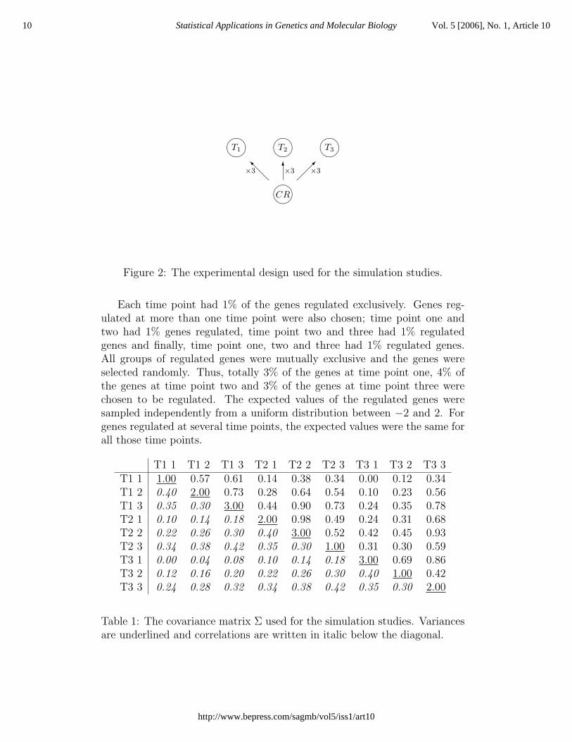
����T1

@@I×3

����T2

6×3

����T3

���×3

����CR

Figure 2: The experimental design used for the simulation studies.

Each time point had 1% of the genes regulated exclusively. Genes reg-ulated at more than one time point were also chosen; time point one andtwo had 1% genes regulated, time point two and three had 1% regulatedgenes and finally, time point one, two and three had 1% regulated genes.All groups of regulated genes were mutually exclusive and the genes wereselected randomly. Thus, totally 3% of the genes at time point one, 4% ofthe genes at time point two and 3% of the genes at time point three werechosen to be regulated. The expected values of the regulated genes weresampled independently from a uniform distribution between −2 and 2. Forgenes regulated at several time points, the expected values were the same forall those time points.

T1 1 T1 2 T1 3 T2 1 T2 2 T2 3 T3 1 T3 2 T3 3T1 1 1.00 0.57 0.61 0.14 0.38 0.34 0.00 0.12 0.34T1 2 0.40 2.00 0.73 0.28 0.64 0.54 0.10 0.23 0.56T1 3 0.35 0.30 3.00 0.44 0.90 0.73 0.24 0.35 0.78T2 1 0.10 0.14 0.18 2.00 0.98 0.49 0.24 0.31 0.68T2 2 0.22 0.26 0.30 0.40 3.00 0.52 0.42 0.45 0.93T2 3 0.34 0.38 0.42 0.35 0.30 1.00 0.31 0.30 0.59T3 1 0.00 0.04 0.08 0.10 0.14 0.18 3.00 0.69 0.86T3 2 0.12 0.16 0.20 0.22 0.26 0.30 0.40 1.00 0.42T3 3 0.24 0.28 0.32 0.34 0.38 0.42 0.35 0.30 2.00

Table 1: The covariance matrix Σ used for the simulation studies. Variancesare underlined and correlations are written in italic below the diagonal.

10 Statistical Applications in Genetics and Molecular Biology Vol. 5 [2006], No. 1, Article 10

http://www.bepress.com/sagmb/vol5/iss1/art10

The total number of genes used was 10000 and the hyperparameter αwas fixed to 2. These values are typical for real datasets. The covariancematrix for the experiment was chosen so that there are moderate correlationsbetween the arrays within time points and low to moderate correlations be-tween arrays from different time points (Table 1). Observations for each geneg were then simulated according to the model.

4.2 Comparison with other methods

To investigate if the assumption of a general covariance matrix results in a sig-nificantly improved performance, WAME was compared to two other meth-ods; the moderated F -statistic (Smyth, 2004) and the ordinary F -statistic.The moderated F -statistic is based on a linear model with an empirical Bayesapproach similar to WAME but variance homogeneity and uncorrelated ar-rays are assumed. This method is available as an R-package called LIMMA(Smyth et al., 2005) and can be retrieved from the Bioconductor repository(Gentleman et al., 2004). Since this package contains a function to calcu-late weights used in the estimation of the expected values, LIMMA was usedboth with and without this feature and will be referred to as weighted andunweighted LIMMA respectively.

First, a test of regulation in time point two was used, i.e. a contrast ma-trix with a single row was used. All methods were applied to the simulatedtime course experiment (as described in Section 4.1) and by counting thenumber of true positives as a function of the number of false positives, Re-ceiver Operating Characteristic (ROC) curves were plotted. The simulationresults (see Figure 3) show that WAME clearly performs better than theother methods. Moreover, the performance in LIMMA is only marginallyimproved when weights are used. The ordinary F -statistic has the worstperformance.

Next, the test of no regulation at any time point was performed andthe corresponding ROC plots were plotted (Figure 4). As in the previoussimulation, WAME performs better than the other methods.

4.3 The effects of correlations between conditions

To investigate the impact of correlations between arrays from different timepoints, the simulated time course experiment was used once more. Thistime, three different versions of WAME were compared, each with the scaledcovariance matrix Σ∗ given instead of estimated. The scale λ and the hyper-parameter α were estimated as usual.

11Kristiansson et al.: Quality Optim. Analysis of General Paired Microarray Experiments

Produced by The Berkeley Electronic Press, 2006

0.0 0.2 0.4 0.6 0.8 1.0

0.0

0.2

0.4

0.6

0.8

1.0

False Positives

Tru

e P

ositi

ves

WAMELIMMAWeighted LIMMAOrdinary FRandom selection

0.00 0.02 0.04 0.06 0.08 0.10

0.0

0.1

0.2

0.3

0.4

0.5

False Positives

Tru

e P

ositi

ves

WAMELIMMAWeighted LIMMAOrdinary FRandom selection

Figure 3: Receiver Operating Characteristic curves for testing regulation attime point two. Four methods are compared on simulated data; WAME,LIMMA with and without weights and the ordinary F -statistic. The figureto the right is a magnification of the dashed box to the left.

0.0 0.2 0.4 0.6 0.8 1.0

0.0

0.2

0.4

0.6

0.8

1.0

False Positives

Tru

e P

ositi

ves

WAMELIMMAWeighted LIMMAOrdinary FRandom selection

0.00 0.02 0.04 0.06 0.08 0.10

0.0

0.1

0.2

0.3

0.4

0.5

False Positives

Tru

e P

ositi

ves

WAMELIMMAWeighted LIMMAOrdinary FRandom selection

Figure 4: Receiver Operating Characteristic curves for testing regulation atall time points. Four methods are compared on simulated data; WAME,LIMMA with and without weights and the ordinary F -statistic. The figureto the right is a magnification of the dashed box to the left.

12 Statistical Applications in Genetics and Molecular Biology Vol. 5 [2006], No. 1, Article 10

http://www.bepress.com/sagmb/vol5/iss1/art10

The first version used the true matrix shown in Table 1, the second versionused the true matrix altered by setting the correlations between groups tozero. Finally, the third version used an identity matrix which results ina model equivalent to the model presented in Smyth (2004) and will thusperform similar to LIMMA. The setup of this simulation is summarised inTable 2.

WAME version 1 True covariance matrix including both differentvariances for different arrays and correlations betweenall pairs of arrays.

WAME version 2 True covariance matrix but all correlations betweenpairs of arrays from different time points set to zero.

WAME version 3 Identity matrix, i.e. same variance for all arrays andno correlations. Equivalent to LIMMA.

Table 2: The experimental setup used in the simulation study to investigatethe impact of the correlations. The result can be seen in Figure 5.

The test used is the same as in the first simulation study, i.e. a testfor regulation in time point two and the results can be seen in Figure 5.As expected, the version with the true covariance matrix performs best,followed by the version with independence between time points and finallythe version which uses an identity matrix. It is interesting to see that theperformance loss when correlations between the time points are ignored, isrelatively large. This shows that a potential method that focuses on each ofthe groups independently will be far from optimal.

5 Results from real data

Here, two real datasets are examined. First, the apoAI dataset (Callowet al., 2000) is analysed, where two-colour spotted cDNA microarrays areused to compare eight knockout mice to eight control mice through a commonreference. Then the Cardiac dataset (Hall et al., 2004) is investigated. Inthis experiment heart biopsies was harvested from 19 patients before andafter treatment with a ventricular assist device. One-channel oligonucleotidemicroarrays from Affymetrix Inc. have been used to create this dataset.

13Kristiansson et al.: Quality Optim. Analysis of General Paired Microarray Experiments

Produced by The Berkeley Electronic Press, 2006

0.0 0.2 0.4 0.6 0.8 1.0

0.0

0.2

0.4

0.6

0.8

1.0

False Positives

Tru

e P

ositi

ves

WAME version 1WAME version 2WAME version 3Random selection

0.00 0.02 0.04 0.06 0.08 0.10

0.0

0.1

0.2

0.3

0.4

0.5

False Positives

Tru

e P

ositi

ves

WAME version 1WAME version 2WAME version 3Random selection

Figure 5: Simulated Receiver Operating Characteristic curves for testingthree versions of WAME, all using given covariance matrices. Version 1 usesthe correct covariance matrix, version 2 uses the correct covariance matrixbut with all correlations between the time points set to zero and finally,version 3 uses an identity matrix.

5.1 The apoAI dataset

The apoAI dataset (Callow et al., 2000) comes from a study of high-densitylipoprotein (HDL) metabolism in mice. In the study, mRNA from eight micewith the apolipoprotein AI gene inactivated were compared to mRNA fromeight control mice through a common reference, which was created by poolingmRNA from the controls (see Figure 6). The samples from the knockouts andcontrols were labeled with Cy3 and the samples from the common referencewere labeled with Cy5. In total, 16 two-channel cDNA microarrays werehybridised.

The pre-processing of this data is described in Callow et al. (2000) andis summarised here. ScanAlyze was used to analyse the scanned arrays andthe background estimation and correction were done in Spot (Buckley, 2000).The resulting files containing background corrected raw intensities are pub-licly available at

http://www.stat.berkeley.edu/users/terry/zarray/Html/apodata.html

Array elements with missing values were removed (totally 158 genes out of6226) and print-tip loess normalisation (Yang et al., 2002) was used to remove

14 Statistical Applications in Genetics and Molecular Biology Vol. 5 [2006], No. 1, Article 10

http://www.bepress.com/sagmb/vol5/iss1/art10

����A

AAK×8

��������×8

����C K

CR

Figure 6: Experimental design for the apoAI dataset. The conditions C andK correspond to the control mice and knockout mice respectively. CR isthe common reference which was created by pooling the mRNA from thecontrols. The mRNA from the control mice and the knockout mice werelabeled with Cy5 and the mRNA from the common reference were labelledwith Cy3. In total 16 arrays were used in this experiment.

systematic errors.In the present paper, the linear model developed in Section 3 will be

used to analyse this dataset. Three conditions are used to parametrise thisexperiment; the control (C), the knockout (K) and the common reference(CR). The contrast of interest is the difference between the knockout andcontrol. Note that due to the experimental design, this dataset could not beanalysed by the simpler model presented in Kristiansson et al. (2005).

WAME was applied to the normalised values and the estimated covariancematrix (see Table 3) reveals differences in the variance structure between thetwo groups. In the first group, which consists of the eight control mice, allarrays have fairly similar variances (between 0.16 and 0.10). In the knockoutgroup however, there are several arrays with quite high variances, e.g. array1 (0.29), array 5 (0.24) and array 6 (0.23).

The estimated covariances are positive for all pairs of arrays. In fact,only a few pair of arrays have a correlation lower than 0.10 and the majorityhave a correlation above 0.20. These correlations can be verified by exami-nation of the high density parts of the clouds in Figure 7. These moderatecorrelations can be a result of the common reference design that is used inthe experiment. By hybridising mRNA from the same pool on all the arrays,sources of variation will undoubtedly be shared.

The weights that correspond to the contrast comparing the knockoutsto the controls are shown in Table 4. As mentioned earlier, the variancein the control group is homogeneous which results in fairly equal weights.In the knock-out group however, the variance and thus the weights differ

15Kristiansson et al.: Quality Optim. Analysis of General Paired Microarray Experiments

Produced by The Berkeley Electronic Press, 2006

Figure 7: Pair-wise plots of the log2-ratios for all the 16 arrays in the apoAIdataset. The lower left half shows kernel density estimates of the two-dimensional distribution according to the colour-scale: white, grey, blackand red (in increasing level of density). A standalone image in the losslessPNG format can be found at http://wame.math.chalmers.se.

16 Statistical Applications in Genetics and Molecular Biology Vol. 5 [2006], No. 1, Article 10

http://www.bepress.com/sagmb/vol5/iss1/art10

c1 c2 c3 c4 c5 c6 c7 c8 k1 k2 k3 k4 k5 k6 k7 k8c1 0.16 0.03 0.04 0.04 0.05 0.02 0.03 0.04 0.08 0.03 0.03 0.04 0.05 0.05 0.05 0.05c2 0.23 0.11 0.05 0.06 0.02 0.04 0.03 0.03 0.04 0.06 0.06 0.02 0.05 0.02 0.02 0.03c3 0.32 0.50 0.11 0.06 0.02 0.05 0.03 0.03 0.04 0.06 0.08 0.02 0.06 0.02 0.02 0.03c4 0.26 0.45 0.52 0.14 0.02 0.04 0.04 0.03 0.04 0.07 0.08 0.02 0.07 0.03 0.02 0.04c5 0.31 0.13 0.15 0.12 0.14 0.03 0.05 0.05 0.07 0.01 0.02 0.04 0.04 0.06 0.08 0.07c6 0.19 0.42 0.44 0.37 0.26 0.10 0.04 0.04 0.03 0.05 0.06 0.02 0.05 0.03 0.03 0.04c7 0.21 0.28 0.29 0.33 0.40 0.39 0.11 0.04 0.04 0.04 0.05 0.02 0.06 0.04 0.05 0.05c8 0.27 0.28 0.28 0.26 0.45 0.41 0.40 0.11 0.06 0.03 0.04 0.03 0.05 0.05 0.06 0.07k1 0.38 0.20 0.25 0.18 0.34 0.19 0.21 0.32 0.29 0.05 0.04 0.06 0.07 0.08 0.08 0.09k2 0.22 0.43 0.50 0.50 0.09 0.42 0.30 0.26 0.24 0.15 0.08 0.03 0.07 0.04 0.02 0.04k3 0.21 0.45 0.59 0.54 0.12 0.47 0.36 0.29 0.21 0.56 0.15 0.02 0.08 0.03 0.02 0.03k4 0.27 0.18 0.19 0.17 0.25 0.12 0.16 0.23 0.29 0.20 0.13 0.15 0.05 0.08 0.04 0.05k5 0.24 0.29 0.38 0.38 0.22 0.30 0.34 0.28 0.27 0.36 0.40 0.28 0.24 0.07 0.05 0.06k6 0.24 0.14 0.15 0.19 0.35 0.22 0.25 0.30 0.30 0.21 0.13 0.43 0.28 0.23 0.07 0.08k7 0.32 0.18 0.20 0.15 0.60 0.28 0.37 0.48 0.41 0.14 0.17 0.29 0.28 0.38 0.14 0.08k8 0.34 0.25 0.21 0.24 0.49 0.35 0.37 0.51 0.44 0.25 0.21 0.32 0.29 0.43 0.55 0.16

Table 3: Estimated covariance matrix for the apoAI dataset. The variancesare underlined and correlations are written in italic below the diagonal.

substantially. Here, the arrays 1, 5 and 6, which all have a large variance,get heavily down-weighted.

Array c1 c2 c3 c4 c5 c6 c7 c8 SumWeights -0.08 -0.09 -0.16 -0.13 -0.15 -0.13 -0.11 -0.16 -1

Array k1 k2 k3 k4 k5 k6 k7 k8 SumWeights 0.01 0.17 0.25 0.10 0.05 0.03 0.23 0.15 1

Table 4: The weights used in testing difference in gene expression betweenthe knockouts and the controls in the apoAI dataset.

For all array elements p-values were calculated for three different meth-ods; the weighted moderated t-statistic (WAME), the moderated t-statistic(LIMMA) and the ordinary t-statistic. The 15 most extreme elements accord-ing to WAME can be seen in Table 5. The first entry in this list correspondsto the removed apoAI gene and it is found to be heavily down-regulated asone would expect. The next seven entries correspond to three other genes,which all have been verified to be differentially expressed (Callow et al.,2000).

Two quantile-quantile plots are shown in Figure 8. To the left, the ob-served t-values from WAME are plotted against the theoretical values underthe null hypothesis. The eight verified elements are marked with crosses andthey clearly stand out compared to the other elements. To the right, a blowup of the dashed box is shown. In this figure, quantile-quantile curves forthe weighted moderated t-statistic (WAME) and the moderated t-statistic(LIMMA) are plotted. WAME seems to follow the diagonal line well while

17Kristiansson et al.: Quality Optim. Analysis of General Paired Microarray Experiments

Produced by The Berkeley Electronic Press, 2006

LIMMA deviate slightly towards higher observed absolute t-values. A simi-lar deviation can also be seen in the quantile-quantile curve of the ordinaryt-statistic (results not shown).

Name Average Ord. t-test LIMMA WAMElog2-ratio p-value p-value p-value

Apo AI, lipid-Img -3.18 1.51× 10−12 4.98× 10−15 6.11× 10−15

Est, highly similar to apolipoprotein A-I precursor, lipid-UG -2.96 1.21× 10−8 1.63× 10−10 2.53× 10−10

Catechol O-Methylthansferase, membrane-bound, brain-Img -1.76 1.21× 10−8 3.14× 10−10 1.95× 10−9

Est, Weakly similar to C-5 Sterol Desaturase, lipid-UG -0.96 3.39× 10−9 7.52× 10−10 5.24× 10−9

Est, Highly similar to Apolipoprotein C-III precursor, lipid-UG -1.01 3.30× 10−7 4.56× 10−8 2.47× 10−8

Apo CIII, lipid-Img -0.90 5.53× 10−8 1.22× 10−8 2.99× 10−8

Est -0.92 3.01× 10−7 4.65× 10−8 6.27× 10−8

Similar to yeast sterol desaturase, lipid-Img -0.94 4.50× 10−6 7.09× 10−7 3.79× 10−7

Similar to Hypothetical protein 1 - fruit fly -0.57 4.62× 10−3 2.63× 10−3 2.52× 10−4

Fatty acid-binding protein, epidermal, lipid-UG -0.48 5.66× 10−4 2.49× 10−4 3.06× 10−4

BLANK 0.44 5.65× 10−3 4.65× 10−3 4.13× 10−4

estrogen rec 0.42 1.43× 10−3 1.03× 10−3 7.10× 10−4

Cy5RT 0.71 4.14× 10−3 1.68× 10−3 1.03× 10−3

Tbx6 -0.33 5.62× 10−3 7.93× 10−3 1.18× 10−3

Est 0.47 1.30× 10−2 9.63× 10−3 1.32× 10−3

Table 5: The 15 genes in the ApoAI dataset with smallest p-values accordingto WAME. The table also shows the corresponding fold-changes and p-valuesfor the ordinary and moderated t-statistics.

To highlight the impact of the generalised linear model used in WAME,the empirical distributions of the weighted mean (WAME) and the ordinary(i.e. unweighted) mean (LIMMA) were compared. Under the model as-sumptions, the weighted mean should have a smaller variance and thus thedistribution should have a smaller spread. This is in fact observed when theempirical distributions are estimated by a kernel density estimator (see Fig-ure 9). This suggests that the estimator of the fold-changes in WAME hashigher precision than the corresponding estimator in LIMMA.

5.2 The Cardiac dataset

In Hall et al. (2004) heart biopsies from 19 patients with heart failure wereharvested to investigate differences in gene expression before and after treat-ment with a ventricular assist device. The role of the study was to identifygenes involved in vascular signaling networks. The patients were dividedinto three groups; the ischemic group (I) with 5 patients that had evidenceof coronary artery disease, the acute myocardial infarction group (IM) with6 patients that had an acute myocardial infarction within 10 days of theimplant and finally the nonischemic group (N) where the 8 patients did notshow any evidence for coronary artery disease. Each mRNA sample wasprepared and hybridised to one Affymetrix one-channel oligonucleotide array

18 Statistical Applications in Genetics and Molecular Biology Vol. 5 [2006], No. 1, Article 10

http://www.bepress.com/sagmb/vol5/iss1/art10

Figure 8: To the left a quantile-quantile plot comparing the estimatedweighted moderated t-statistic (WAME) to its corresponding theoretical nulldistribution. The eight elements marked with a cross corresponds to the fourgenes that were verified to be differentially expressed. To the right is a blowup of the dashed box. This plot also contains the quantile-quantile curve forthe moderated t-statistic (LIMMA).

Figure 9: Kernel density estimates of the distributions of the mean valuesfrom WAME and LIMMA. The spread of the former is smaller which suggeststhat the estimator in WAME is more precise.

19Kristiansson et al.: Quality Optim. Analysis of General Paired Microarray Experiments

Produced by The Berkeley Electronic Press, 2006

(HG-U133A) resulting in two arrays for each patient, i.e. 38 arrays in total.The resulting raw data was made publically available by the authors and canbe found at the Gene Expression Omnibus repository (Edgar et al., 2002).

The .CEL-files for all 38 arrays were retrieved and then pre-processed andnormalised by RMA (Irizarry et al., 2003). The paired observations were usedto form log2-ratios according to the experimental design shown in Figure 10.The ischemic group (I) of this dataset was analysed in Kristiansson et al.(2005) where patients with different variances and substantial correlationswere identified.

In the present paper the ischemic group will be analysed once more, butthis time using the more general model. In this framework, all patients willbe incorporated, even if we only test for differential expression for patientsin a single group. This is a major difference to the model in Kristianssonet al. (2005) which can only take advantage of the arrays from one group ofinterest, i.e. it can only analyse direct comparisons with two conditions. Inthis section, the results from the new analysis are presented and comparedto the corresponding old results.

After

Before ����IB

����

IA

?×5

����IMB

����IMA

?×6

����NB

����NA

?×8

Figure 10: Experimental design for the cardiac dataset. All three groups havea condition before the treatment (IB, IMB and NB) and a condition afterthe treatment (IA, IMA and NA). The dataset consists of 19 observations intotal.

The estimated covariance matrix for all 19 pairs of arrays is shown inTable 6. The variances in this dataset differ considerable, both between andwithin the three groups. For example, the IM group has three arrays withhigh variance and three arrays with rather low variance, while the variancesin I and N group are more homogeneous.

The correlations in this dataset are in general small, but there are ex-ceptions. The first patient in the IM group (IM1) has a high positive cor-relation with IM4 (0.54) but also negative correlations with I7 (−0.64) andIM7 (−0.55). These correlations can also be seen in Figure 11. A closer

20 Statistical Applications in Genetics and Molecular Biology Vol. 5 [2006], No. 1, Article 10

http://www.bepress.com/sagmb/vol5/iss1/art10

I12 I13 I4 I7 I8 IM1 IM3 IM4 IM5 IM6 IM7 N2 N22 N3 N4 N6 N7 N8 N9I12 0.04 0.00 0.00 0.01 0.00 -0.01 0.01 -0.00 -0.01 0.00 0.01 -0.01 0.00 0.01 0.00 0.01 -0.00 0.00 0.01I13 0.03 0.17 -0.01 0.01 -0.00 0.10 0.11 0.08 0.07 0.02 -0.05 0.01 -0.06 -0.01 0.03 -0.02 -0.06 -0.05 0.01I4 0.04 -0.13 0.06 0.01 0.00 -0.03 0.00 -0.01 -0.01 0.00 0.02 -0.01 0.01 0.00 0.01 0.02 -0.01 0.02 -0.00I7 0.11 0.07 0.09 0.23 -0.02 -0.26 0.07 -0.04 0.03 -0.01 0.04 -0.06 0.01 -0.00 0.02 0.05 -0.03 0.05 0.01I8 0.03 -0.02 0.04 -0.16 0.04 0.04 -0.02 0.01 -0.00 0.00 -0.00 0.01 0.00 0.01 -0.00 0.00 0.01 -0.01 0.00

IM1 -0.04 0.29 -0.15 -0.64 0.22 0.73 -0.06 0.18 0.10 0.06 -0.14 0.14 -0.07 0.02 -0.02 -0.10 -0.04 -0.18 0.00IM3 0.11 0.41 0.02 0.22 -0.12 -0.11 0.43 0.04 -0.04 0.02 -0.02 -0.07 -0.04 -0.01 0.06 -0.01 -0.06 -0.01 0.03IM4 -0.01 0.50 -0.06 -0.24 0.12 0.54 0.17 0.14 0.07 0.02 -0.04 0.02 -0.04 -0.01 0.00 -0.00 -0.04 -0.05 0.01IM5 -0.09 0.29 -0.05 0.09 -0.00 0.19 -0.09 0.32 0.35 0.01 -0.03 0.05 -0.03 -0.01 -0.00 0.03 -0.03 -0.05 -0.00IM6 0.10 0.20 0.02 -0.13 0.08 0.29 0.15 0.22 0.06 0.06 -0.01 0.00 -0.01 0.01 0.00 -0.01 -0.01 -0.02 0.00IM7 0.09 -0.41 0.27 0.31 -0.06 -0.55 -0.09 -0.39 -0.20 -0.20 0.08 -0.03 0.03 0.01 0.00 0.04 0.03 0.05 -0.00N2 -0.12 0.06 -0.08 -0.29 0.10 0.40 -0.25 0.15 0.22 0.05 -0.28 0.17 -0.01 0.00 -0.02 -0.02 -0.01 -0.05 -0.01

N22 0.04 -0.49 0.12 0.04 0.02 -0.28 -0.20 -0.36 -0.19 -0.08 0.38 -0.10 0.09 0.01 -0.01 0.01 0.03 0.02 -0.00N3 0.11 -0.10 0.04 -0.01 0.14 0.07 -0.04 -0.06 -0.05 0.10 0.09 0.03 0.20 0.06 -0.00 0.00 0.01 -0.00 0.01N4 0.03 0.20 0.08 0.12 -0.03 -0.08 0.28 0.04 -0.01 0.04 0.05 -0.11 -0.08 -0.02 0.10 0.01 -0.01 0.01 0.00N6 0.09 -0.14 0.21 0.30 0.03 -0.35 -0.03 -0.04 0.14 -0.13 0.36 -0.15 0.13 0.03 0.10 0.11 0.02 0.05 0.01N7 -0.06 -0.41 -0.07 -0.18 0.07 -0.15 -0.27 -0.27 -0.15 -0.14 0.28 -0.04 0.31 0.14 -0.05 0.16 0.12 0.03 -0.01N8 0.01 -0.28 0.20 0.21 -0.06 -0.46 -0.03 -0.27 -0.17 -0.17 0.41 -0.28 0.16 -0.04 0.04 0.36 0.21 0.20 -0.01N9 0.26 0.13 -0.01 0.09 0.06 0.02 0.22 0.10 -0.01 0.00 -0.01 -0.08 -0.04 0.09 0.06 0.10 -0.12 -0.05 0.05

Table 6: Estimated covariance matrix for the cardiac dataset. The variancesare underlined and correlations are written in italic below the diagonal.

examination of the log2-ratios revealed that both IM1 and I7 have skeweddistributions, IM1 towards positive values and I7 towards negative values.This may be a result from either the experiment itself or from pre-processingsteps and can explain the unexpected negative correlations. However, wewill still keep these arrays in the further analysis, since their high variancewill result in a low weight and thus a low impact on the final result. Thehyperparameter α was estimated to 1.73 which means that the resulting t-distribution will gain approximately 3.5 degrees of freedom.

The weights used in the test for differential expression in group I canbe seen in Table 7. Not surprisingly, the patient I7 gets the lowest weight,while I12 and I8, which both have low variance and small correlations, getthe highest weights. Note that these weights sum to 1.

It is also interesting to examine the weights in the IM and N group. Dueto correlations between patients from different groups, these weights will benon-zero but sum to zero. Due to the high variances in the IM group, thecorresponding weights are relatively low. In the N group, N7 and N6 haverelatively high weights (0.10 and −0.06), which stems from that the factthat they both have a low variance and correlates with group I (N7 mostlynegative and N6 mostly positive).

To test for differential expression in group I, the weighted moderated t-statistic was calculated. Figure 12 show the resulting quantile-quantile plotwhere the theoretical t-distribution has approximately 19.5 degrees of free-dom. Most genes follow the diagonal line well which suggest relatively fewregulated genes and a good model fit. A few genes have a larger absolutet-value than can be explained by the null distribution which points towards

21Kristiansson et al.: Quality Optim. Analysis of General Paired Microarray Experiments

Produced by The Berkeley Electronic Press, 2006

Figure 11: Pair-wise plots of the log2-ratios for all the 19 patients in thecardiac dataset. The lower left half shows kernel density estimates of thetwo-dimensional distribution according to the colour-scale: white, grey, blackand red (in increasing level of density). A standalone image in the losslessPNG format can be found at http://wame.math.chalmers.se.

22 Statistical Applications in Genetics and Molecular Biology Vol. 5 [2006], No. 1, Article 10

http://www.bepress.com/sagmb/vol5/iss1/art10

Patient I12 I13 I4 I7 I8 SumWeight 0.28 0.13 0.21 0.10 0.28 1Patient IM1 IM3 IM4 IM5 IM6 IM7 SumWeight 0.03 -0.01 -0.02 -0.00 -0.01 0.01 0Patient N2 N22 N3 N4 N6 N7 N8 N9 SumWeight 0.03 0.05 -0.05 -0.02 -0.06 0.10 0.01 -0.05 0

Table 7: Weights for the patients in the cardiac dataset when differentialexpression in the ischemic (I) group is studied.

some of them being regulated. Note that the gene expression in this experi-ment is asymmetric with more genes seemingly up-regulated than seeminglydown-regulated.

Figure 12: This figure shows the quantile-quantile plots of the weighted mod-erated t-statistic for the test of differential expression in group I.

When the results are compared to the corresponding analysis restrictedto the arrays from group I (the analysis in Kristiansson et al. (2005)) thereare both similarities and differences. The estimated scaled covariance matrixfor the 5 patients in group I are similar and both the scaled variances andthe correlations above 0.10 change less than 10%. The hyperparameter α isestimated to 1.92 when only the patients from group I are used instead of1.73 when all 19 patients are used. This results in a slightly different scalingfactor λ (0.046 instead of 0.042) and thus a different covariance matrix.

23Kristiansson et al.: Quality Optim. Analysis of General Paired Microarray Experiments

Produced by The Berkeley Electronic Press, 2006

Moreover, there are interesting differences between the weights from thetwo models. Under the general model (Table 7), the weights are more con-servative than under the restricted model (Table 8). For example, the weightfor patient I7 increases from 0.05 to 0.10.

Patient I12 I13 I4 I7 I8 SumWeight 0.30 0.09 0.23 0.05 0.33 1

Table 8: The weights from the I group calculated by the old model in Kris-tiansson et al. (2005). These weights are less conservative than the weightsin Table 7.

Ranking lists sorted by the p-values were produced for both models.Among the top 100 and 500 genes, 38% and 52% respectively, appear onboth lists. To compare the deviating genes, quantile-quantile plots of thep-values on a logarithmic scale (base 10) were made (Figure 13). In the plotto the left (general model), fewer genes deviate from the diagonal line than inthe plot to the right (restricted model). Since the number of regulated genesis unknown it is hard to say which plot that is more correct but a betteroverall fit makes the extreme genes more distinct.

6 Discussion

The experimental design of microarray gene expression assays are often com-plex and several conditions are usually involved. The arrays in these exper-iments are produced through a series of steps, each inducing differences inprecision and systematic effects. This generates data with varying quality,which is desirable to take into account.

In this paper, a generalisation of the paired two-sample analysis methodintroduced in Kristiansson et al. (2005) is described. The new method, whichas its predecessor, is referred to as WAME, is based on a linear model capableof analysing paired microarray experiments with any number of conditions.The observations are assumed to measure the differences in mRNA levelson a logarithmic scale (log-ratios) between pairs of conditions. This meansthat the method will be applicable to most experiments using two-channelcDNA microarrays and many experiments with one-channel oligonucleotidemicroarrays from Affymetrix.

For each gene, the vector of all the pair-wise log-ratios are assumed tofollow a multidimensional normal distribution. A covariance matrix Σ is used

24 Statistical Applications in Genetics and Molecular Biology Vol. 5 [2006], No. 1, Article 10

http://www.bepress.com/sagmb/vol5/iss1/art10

Figure 13: This figure shows two quantile-quantile plots of the log10 p-valuesfor the test of differential expression in group I. The plot to the left is basedon the general paired model using all 19 patients and the plot to the right isbased on the restricted model from Kristiansson et al. (2005) using only thepatients in the I group.

to catch the differences in quality of the different pairs, such as correlationsand unequal precision. Gene-specific variances are modelled through a factorcg, scaling the covariance matrix uniquely for each gene. Since microarrayexperiments often consist of few gene-wise repetitions, cg is modelled by aninverse gamma distribution random variable with shape parameter α andfixed scale parameter β. This is analogous to Lonnstedt and Speed (2002),Smyth (2004) and Kristiansson et al. (2005).

To estimate the covariance matrix Σ, an assumption that most genes arenot differentially expressed is made. Then, after cg is removed by a trans-formation, Σ scaled with an unknown scale λ can be estimated by numericalmaximum likelihood. Point estimators for λ and α are also derived basedon the residual sum of squares. All these steps parallel Kristiansson et al.(2005).

For any testable linear hypotheses, a likelihood ratio test is derived, re-sulting in a weighted moderated F -statistic. In the special case of a one-dimensional null hypothesis restriction, a weighted moderated t-statistic isformed. In both cases, correlations give rise to array-specific weights, thatcan be non-zero for parts of the data that would not be included under theassumption of independent arrays. The weighted moderated statistics can be

25Kristiansson et al.: Quality Optim. Analysis of General Paired Microarray Experiments

Produced by The Berkeley Electronic Press, 2006

seen as generalisations of the moderated F - and t-statistics found in Smyth(2004).

The model was evaluated on a simulated time course experiment withthree time points. The improvement in performance, compared to LIMMA(Smyth et al., 2005) was shown to be substantial. Moreover, when the timepoints were (wrongly) assumed to be independent, the effect on the perfor-mance was shown to be relatively large.

Two real datasets were analysed. The first was the apoAI dataset (Cal-low et al., 2000) which consists of eight knockout mice that are comparedto eight controls through a common reference. The estimated covariancematrix contains moderate positive correlations for almost all arrays. This isprobably a result of the common reference design, where sources of variationundoubtedly are shared between the arrays. Quantile-quantile plots of thet-statistic revealed that WAME fitted the diagonal line well, while LIMMAtended to over-estimate the t-values. A similar effect was observed for themodel in (Kristiansson et al., 2005). Moreover, the precision for the esti-mated fold-changes was shown to increase when variances and covarianceswere taken into account.

The other dataset investigated was the cardiac dataset (Hall et al., 2004)which contains paired measurements for 19 patients, divided into three groups(I, IM and N) based on their medical condition. One-channel oligonucleotidemicroarrays from Affymetrix were used to produce the data. The covariancematrix revealed differences between the groups. The variances were homo-geneous in both the I and N group in contrast to the IM group where bothhigh and low variances were found. The IM group also contained several highcorrelations, both to patients within the group and to patients in the othergroups.

Differential expression in the first group was investigated and the resultscompared to Kristiansson et al. (2005). The weights with the general modelsuggested in this paper resulted in more conservative weights and quantile-quantile plots for the p-values showed that fewer genes deviated from thediagonal.

When using WAME, it is important to keep in mind that the model isfar from perfect. The noise structure may be different for different genes andthe assumption of normality may not be valid. The gene-specific variancemight also be different for different groups of conditions, leading to erroneousvariance estimates. The effect of a potential dependence between expressionlevel and variance is unknown.

In principle we may adapt the weighted moderated F - or t-tests to testnull hypotheses that the linear combinations in question are equal to arbitrary

26 Statistical Applications in Genetics and Molecular Biology Vol. 5 [2006], No. 1, Article 10

http://www.bepress.com/sagmb/vol5/iss1/art10

constants. Confidence intervals and ellipsoids can then be constructed basedon the correspondence theorem between hypothesis testing and confidencesets (Casella and Berger, 2002, Theorem 9.2.2). However, since the assumedvariance structure is hard to validate for regulated genes, we have refrainedfrom developing this topic at this stage.

It should also be noted that the restriction to models with pairwise ob-servations in Section 2.1 may be relaxed. A crucial step, preceding the hy-pothesis testing in Section 3.3, is the estimation of the covariance matrixin Section 3.1 where we assume that the expected value of the observationvector Xg has approximately mean zero for a majority of genes. This seemsreasonable if Xg consists of pair-wise differences as assumed in Section 2.1leading to a design matrix with row sums zero, but the assumption may alsobe satisfied in other designs such as in some regression models.

A further generalisation of WAME is currently being developed, extend-ing the procedure from paired to general microarray experiments. A lineartransformation can there be used to first remove the information explainableby the null hypothesis. Assuming that the null hypothesis is true for mostgenes, the transformed covariance structure can then be estimated and theweighted statistics formed from the transformed data similar to the meth-ods in the current paper. Work is underway to derive the properties of thisprocedure and to verify its usefulness on real data. An R-package providingeasy access to the WAME procedure is also under development.

References

S.F. Arnold. The Theory of Linear Models and Multivariate Analysis. JohnWiley & Sons, 1980.

P. Baldi and A.D. Long. A Bayesian framework for the analysis of microar-ray expression data: regularized t-test and statistical inferences of genechanges. Bioinformatics, 17(6):509–519, 2001.

M.J. Buckley. Spots User’s Guide. CSIRO Mathe-matical and Information Sciences, Sydney, Australia.http://www.cmis.csiro.au/iap/Spot/spotmanual.htm, 2000.

M.J. Callow, S. Dudoit, E.L. Gong, T.P. Speed, and E.M. Rubin. Microar-ray expression profiling identifies genes with altered expression in HDLdeficient mice. Genome Research, 10(12):2022–2029, 2000.

G. Casella and R.L. Berger. Statistical Inference. Duxbury, 2002.

27Kristiansson et al.: Quality Optim. Analysis of General Paired Microarray Experiments

Produced by The Berkeley Electronic Press, 2006

G.A. Churchill. Fundamentals of experimental design for cdna microarrays.Nature Genetics Supplement, 32:490–495, 2002.

R. Edgar, M. Domrachev, and A.E. Lash. Gene Expression Omnibus: NCBIgene expression and hybridization array data repository. Nucleic AcidsResearch, 30(1):207–210, 2002.

R.C. Gentleman, V.J. Carey, D.M. Bates, B. Bolstad, M. Dettling, S. Du-doit, B. Ellis, L. Gautier, Y. Ge, J. Gentry, K. Hornik, T. Hothorn, W. Hu-ber, S. Iacus, R. Irizarry, L. Friedrich, C. Li, M. Maechler, A.J. Rossini,G. Sawitzki, C. Smith, G. Smyth, L. Tierney, J.Y.H. Yang, and J. Zhang.Bioconductor: Open software development for computational biology andbioinformatics. Genome Biology, 5:R80, 2004.

J.L. Hall, S. Grindle, X. Han, D. Fermin, S. Park, Y. Chen, R.J. Bache,A. Mariash, Z. Guan, S. Ormaza, J. Thompson, J. Graziano, S.E.de Sam Lazaro, S. Pan, R.D. Simari, and L.W. Miller. Genomic pro-filing of the human heart before and after mechanical support witha ventricular assist device reveals alterations in vascular signaling net-works. Journal of Physiological Genomics, 17(3):283–291, 2004. URLhttp://www.ncbi.nlm.nih.gov/geo/query/acc.cgi?acc=GDS558.

R.A. Irizarry, B.M. Bolstad, F. Collin, L.M. Cope, B. Hobbs, and T.P. Speed.Summaries of Affymetrix GeneChip probe level data. Nucleic Acids Re-search, 31(4):e15, 2003.

K. Johnson and S. Lin. QA/QC as a pressing need for microarray analysis:meeting report from CAMDA’02. BioTechniques, 34(suppl):S62–S63, 32003.

N.L. Johnson, S. Kotz, and N. Balakrishnan. Continuous Univariate Distri-butions Volume 2. Wiley, 1995.

E. Kristiansson, A. Sjogren, M. Rudemo, and O. Nerman. Weighted analysisof paired microarray experiments. Statistical Applications in Genetics andMolecular Biology, 4(1):Article 30, 2005.

I. Lonnstedt and T. Speed. Replicated microarray data. Statistica Sinica, 12(1):31–46, 2002.

R Development Core Team. R: A language and environment for statisti-cal computing. R Foundation for Statistical Computing, Vienna, Austria,2004. URL http://www.R-project.org.

28 Statistical Applications in Genetics and Molecular Biology Vol. 5 [2006], No. 1, Article 10

http://www.bepress.com/sagmb/vol5/iss1/art10

G.K. Smyth. Linear models and empirical Bayes methods for assessing dif-ferential expression in microarray experiments. Statistical Applications inGenetics and Molecular Biology, 3(1), 2004.

G.K. Smyth, N.P. Thorne, and J. Wettenhall. LIMMA: Linear Models for Mi-croarray Data User’s Guide, 2005. URL http://www.bioconductor.org.

J.P. Steibel and J.M. Rosa. On reference designs for microarray experiments.Statistical Applications in Genetics and Molecular Biology, 4(1), 2005.

Y.L. Tong. The Multivariate Normal Distribution. Springer, 1990.

Y.H. Yang, S. Dudoit, P. Luu, D. Lin, V. Peng, J. Ngai, and T.P. Speed.Normalization for cDNA microarray data: a robust composite methodaddressing single and multiple slide systematic variation. Nucleic AcidsResearch, 30(4):e15, 2002.

29Kristiansson et al.: Quality Optim. Analysis of General Paired Microarray Experiments

Produced by The Berkeley Electronic Press, 2006

Paper 3

Weighted analysis of general microarray experiments

Anders Sjogren∗1,2, Erik Kristiansson1,2 , Mats Rudemo1,2 , Olle Nerman1,2

1Mathematical Statistics, Chalmers University of Technology, 412 96 Goteborg, Sweden2Mathematical Statistics, Goteborg University, 412 96 Goteborg, Sweden

Email: Anders Sjogren∗- anders.sjogren@math.chalmers.se; Erik Kristiansson - erikkr@math.chalmers.se; Mats Rudemo -

rudemo@math.chalmers.se; Olle Nerman - nerman@math.chalmers.se;

∗Corresponding author

Abstract

Background: In DNA microarray experiments, measurements from different biological samples are often

assumed to be independent and to have identical variance. For many datasets these assumptions have been

shown to be invalid and typically lead to too optimistic p-values. A method called WAME has been proposed

where a variance is estimated for each sample and a covariance is estimated for each pair of samples. The

current version of WAME is, however, limited to experiments with paired design, e.g. two-channel microarrays.

Results: The WAME procedure is extended to general microarray experiments, making it capable of handling

both one- and two-channel datasets. Two public one-channel datasets are analysed and WAME detects both

unequal variances and correlations. WAME is compared to other common methods: fold-change ranking,

ordinary linear model with t-tests, LIMMA and weighted LIMMA. The p-value distributions are shown to differ

greatly between the examined methods. In a resampling-based simulation study, the p-values generated by

WAME are found to be substantially more correct than the alternatives when a relatively small proportion of the

genes is regulated. WAME is also shown to have higher power than the other methods. WAME is available as

an R-package.

Conclusions: The WAME procedure is generalized and the limitation to paired-design microarray datasets is

removed. The examined other methods produce invalid p-values in many cases, while WAME is shown to

produce essentially valid p-values when a relatively small proportion of genes is regulated. WAME is also shown

to have higher power than the examined alternative methods.

1

Background

Introduction

The DNA microarray technique involves a series of steps, from the harvesting of cells or biopsies to the

preprocessing of the scanned arrays, before analysable data are obtained. During several of these steps the

quality can be affected by random factors. For instance, depending on the handling of a biological sample

the mRNA can be more or less degraded [1], and the cell-type composition of a biopsy can be more or less

representative for the tissue in question. When arrays share sources of variation the deviations from the

nominal value will be correlated. For example, two arrays from sources with degraded RNA will both tend

to underestimate the expression of easily degradable genes, and two biopsies with a similar and

non-representative cell-type composition will deviate in a similar fashion from the average expression for

the ideal cell-type composition.

The procedure Weighted Analysis of Microarray Experiments (WAME) [2,3] introduced a model where a

covariance-structure matrix common for all genes aims at catching differences in quality by differences in

variances and covarying deviations by correlations between arrays. For computations of test statistics and

estimators this resulted in weighting of observations according to the estimated covariance-structure

matrix, giving lower weight to imprecise or positively correlated arrays.

In order for the estimation of the covariance matrix to work in the current WAME method, the

measurements of most genes must only measure noise, i.e. have an expected value of zero. This is the case

in experiments where pair-wise log-ratios are observed and where few genes are differentially expressed

between any of the pairwise measured conditions. In the present paper, this crucial constraint will be

relaxed to only require that most genes are non-differentially expressed between the conditions actually

being compared. Thus, non-paired experiments can be analysed, e.g. many additional ones based on

one-channel microarray data. The relaxation is realised by transforming the data to remove irrelevant

information in a manner yielding transformed data with expectation zero for non-differentially expressed

genes, after which the current WAME method is applied. The transformed data are shown to give

equivalent tests and estimates to those of the original data, given the corresponding covariance-structure

matrices.

2

Problem formulation and current methods

Given a microarray experiment with n arrays and m genes, we observe for each gene g an n-dimensional

vector Xg of log2 transformed values measuring mRNA abundance. In WAME the vector Xg is assumed to

have expectation µg described by a design matrix D and a gene-specific parameter vector γg, typically

having one dimension per studied condition. A covariance-structure matrix Σ, common for all genes, is

used to model differences in quality between arrays as different variances and shared sources of variation

between arrays as correlations. A gene-specific variance-scaling factor cg is assumed to have inverse gamma

prior distribution with a global shape parameter α. Conditional on cg the vector Xg is assumed to have a

normal distribution with covariance matrix cgΣ. A matrix C specifies the differential expression vector δg,

describing the linear combinations of the parameters that are of main interest. Formally,

µg = D γg ,

Xg | cg ∼ N(µg, cgΣ) ,

cg ∼ Γ−1(α, 1) ,

(1)

and variables corresponding to different genes are assumed independent. We want to estimate the

differential expression

δg = C γg (2)

or we want to test for differential expression

H0 : δg = 0

HA : δg 6= 0 .(3)

In the current version of WAME [2,3] the estimation of the covariance-structure matrix Σ is based on a

temporary assumption of expectation zero, µg = 0, for all genes, which is shown to give reasonable results

if the expectation is close to zero for most genes. Thus, this is a suitable assumption for data with paired

observations and few regulated genes between the pair-wise measured conditions.

The WAME model can be compared with the ordinary linear model (OLM) [4],

Xg ∼ N(µg, cgI) (4)

which gives rise to the ordinary t- or F-tests, and with a widely used empirical Bayes model proposed in [5]

and implemented in the LIMMA package [6],

Xg | cg ∼ N(µg, cgI) ,

cg ∼ Γ−1(α, β) .(5)

3

The novel feature of WAME was thus the introduction of the quality modelling covariance-structure matrix

Σ.

After the introduction of WAME, a weighted version of LIMMA was proposed [7], which we will refer to as

wLIMMA. There, a model with array-wise variance scales but no correlations is used,

Xg | cg ∼ N(µg, cgdiag(σ21 , . . . , σ2

n)) ,

cg ∼ Γ−1(α, β) .(6)

The parameters are estimated using a restricted maximum-likelihood (REML) approach.

A widely used approach is to only consider the ordinary least-squares estimated differential expression,

often referred to as the log fold-change, here abbreviated as FC, or as the average M-value. In the present

paper, the ranking of the genes imposed by this method will be included in comparisons, when applicable.

Results

The new version of WAME

In the current version of WAME [2,3] the covariance-structure matrix Σ is estimated using a temporary

assumption that µg = 0 for most genes, i.e. that the measurements of most genes consist solely of

biological and technical noise. In the new version of WAME we relax this to only assume that most genes

are non-differentially expressed, i.e. δg = 0. This allows a much larger class of experimental designs and

design matrices D, most notably unpaired designs.

The trick used is to transform the data and consider

Yg = Xg −µ0g (7)

where µ0g is a suitable linear estimator of µg which is unbiased under H0 and which preserves the

estimability of the differential expression δg, based on only the transformed data (see Methods for details).

An example is (8) below where for each gene the mean value of all arrays is subtracted.

Since the transformed data contain only noise for non-differentially expressed genes by construction, the

current version of WAME can essentially be applied to the transformed data Yg. As before, the

covariance-structure matrix (now ΣY ) and the hyperparameter α are first estimated under a provisional

assumption (now δg = 0). The maximum likelihood estimates of δg and the likelihood ratio test statistics

of (3) are then computed. The tests and estimators are in fact unchanged by the transformation (7), if the

4

covariance-structure matrices for the transformed and untransformed data are known (details given in

Methods). WAME is implemented as a package for the R language [8] and is available at

http://wame.math.chalmers.se/ .

Evaluation on real and resampled data

To investigate the properties of the new version of WAME, two real datasets are examined. Briefly, they

are analysed both using WAME and the current methods described in Background. Array-specific weights,

p-value distributions and rankings are produced showing clear differences between the procedures, most

notably in the p-value distributions. To investigate the power of the different procedures and to look at

p-value distributions in a controlled but realistic setting, we also analyse simulated data with real noise

from the studied datasets and synthetic signal.

Description of the real datasets

Two public one-channel microarray datasets are analysed. The datasets are selected from the NCBI GEO

database [9] with the criteria of having unpaired design and being sufficiently large to allow for the

resample-based simulations in Resampled data below.

In the first dataset [10], biopsies were taken from the left atrium from 20 human hearts with normal sinus

rythm and 10 hearts with permanent atrial fibrillation. It is here referred to as Atrium. In the second

dataset [11], mechanisms in chronic obstructive pulmonary disease, COPD, were investigated by taking

lung tissue biopsies from 12 smokers with mild or no emphysema and from 18 smokers with severe

emphysema. In both datasets one Affymetrix HGU-133A array was used for each patient. In the present

paper RMA [12] is used to obtain expression measures from the raw probe-wise intensities. The analyses

are performed using the R language and the Bioconductor framework [13] .

5

Analysis of the real datasets

A natural parameterisation of the included datasets is to have one parameter per condition, yielding design

and hypothesis matrices

D =

1 0...

...1 00 1...

...0 1

and C =

[−1 1

].

Under the null hypothesis, for each gene g and array i, an unbiased estimator of the expected value of the

measurement Xig is obtained by the gene-wise mean value over all arrays from both groups. The

transformation then becomes a subtraction of that mean value, cf. (7),

Yig = Xig −1n

n∑j=1

Xjg . (8)

Note how the transformation preserves the difference in mean value between the two groups of arrays.

If the elements in Xg from the different arrays had in fact independent and identically distributed noise for

each fixed gene g as assumed in OLM and unweighted LIMMA, the noise in Yg would have equal variances

for all arrays. In Figure 1 array-wise density estimates for the transformed expression values are shown. For

arrays from the same condition the distributions should be identical, reflecting the combined variability of

signal and noise. For unregulated genes the expectation of Yg is zero, so if the assumption of few regulated

genes holds the densities from all arrays should furthermore be essentially equal. Examination of Figure 1

reveals that neither of these statements are true, indicating that some variances are highly unequal.

Analogously, all pairs of arrays within each condition should have a common joint distribution and when

few genes are regulated all pairs of arrays should essentially have a common joint distribution with a small

negative correlation of −1/(n− 1). Examination of scatter plots for all pairs of arrays shows that this is

clearly not the case (some obvious examples are shown in Figure 2).

As expected from the observations above, unequal variances and non-zero correlations are estimated in the

analyses with WAME, giving rise to highly unequal weights in the estimates of the differential expressions

(shown in Table 1). In fact, the sign of the weight for some arrays even get switched compared to the sign

of the weight of the other arrays from the same condition. This is an effect of strong correlations combined

with unequal variances. It is an issue which is further addressed in Discussion.

6

The analysis methods described in Background are applied to the data and p-values and ranks computed.

The respective probability plots are shown in Figure 3, demonstrating that there are substantial differences

in the distribution of p-values between the different statistics. Since correlations and unequal variances are

observed, the model assumptions of the alternative standard methods do not seem to hold. The p-values

could thereby have become optimistic. On the other hand, it cannot be ruled out that the temporary

assumption in WAME of no regulated genes makes its p-values conservative, which could also partly

explain the differences. These problems are studied below by use of resampled data.

A common alternative to using the p-values as measures of significance is to consider the ranking of the

genes, induced by the p-values or test statistics, and to select a fixed number of top ranked genes for

further investigations. In Table 2 the concordance of the ranked lists are shown. The results from the

included methods differ, for instance those from WAME compared to the other methods. This is not

surprising since high correlations and highly unequal variances were identified by WAME, giving rise to

highly unequal weights.

Resampled data

To examine closer the effect of violated assumptions of independence and identical distribution, we

repeatedly selected two random subgroups of four arrays from within one group in the original data and

performed tests between those groups. This was performed 100 times for the largest group in each of the

two real datasets. Differentially expressed genes have unequal expected values in the two populations being

sampled (cf. (2)). Since we now sample twice from the same condition, no differentially expressed genes

exist.

Figure 4 shows the empirical p-value distributions for the resampled COPD data analysed with the four

methods, together with the respective average empirical distribution,

F (p) =1

100

100∑i=1

Fi(p) ,

where Fi denotes the empirical CDF from the ith of the 100 resamples. For WAME, the p-value

distributions are very close to the expected uniform. For OLM, LIMMA and weighted LIMMA there is a

high variability between the p-value distributions and they are in many cases substantially different from

the expected uniform. For WAME, OLM and LIMMA, the respective average empirical distribution is

approximately correct, while for weighted LIMMA it is clearly optimistic. The results for the Atrium

7

dataset (data not shown) are very similar.

Evaluation of power

To evaluate the power of the tests in the studied datasets, a known regulation is added to randomly

selected genes in one of the resampled groups, created according to the previous section. Thus, the noise is

obtained from the real data and only the signal is synthetic. Ideally, the power can then be estimated by

the proportion of differentially expressed genes that have a computed p-value less than a fixed level.

However, valid p-values of the test statistics cannot be obtained from the respective models since, as

demonstrated above, the corresponding assumptions are typically not valid. Ideally, the p-values would be

determined by the true null distribution of the respective test statistics, given the array-wise quality

deviations. In the simulation study, the critical value of the test statistics are therefore estimated from the

empirical distribution of the test statistic for the unregulated genes. This is used to estimate the power of

the different statistics (details are given in Methods).

The power estimates for the different methods are shown in Figure 6, for a level 0.1% test. The 0.1% level

yields approximately 22 false positives if relatively few genes are in fact differentially expressed. For

WAME, Σ is estimated both before and after adding a signal to 2228 genes (10%), thereby substantially

affecting the estimate of Σ (cf. Figure 5). The powers of the two versions are nevertheless very similar

(difference less than 0.003) and only the latter version is included in the plot.

When the covariance-structure matrix Σ is estimated in WAME it is assumed that no genes are

differentially expressed. Figure 5 includes the average empirical distribution for the p-values of the

unregulated genes when different proportions of the genes have a log2 differential expression of 1. It is clear

that the distributions are biased for high proportions, giving conservative p-values, which should be an

effect of biased estimates of Σ.

The results from the studied datasets indicate (i) that WAME offers a relevant power increase compared to

the included alternatives, (ii) that weighted LIMMA does not offer an advantage compared to LIMMA and

(iii) that the moderated statistics (WAME, LIMMA and wLIMMA) are superior to the traditional

methods of ranking by ordinary t-statistic (OLM) or estimated differential expression (FC).

8

Discussion

The WAME model and the simulations

The WAME model aims at catching quality deviations by one covariance-structure matrix common for all

genes. This is certainly simplistic in some cases, e.g. when only certain physical parts of an array or certain

types of mRNAs are of decreased quality. The estimated covariance structure can then only be expected to

reflect a mixture of the qualities of the different genes. However, examining the simulations (Figure 6), we

see a clear power gain in the WAME model compared to the other models. Also, WAME succeeds in

catching enough of the quality deviations to make the p-value distributions more correct, thus providing

increased usefulness of the p-values (Figure 3).

The models of LIMMA, weighted LIMMA and WAME are nested, where weighted LIMMA adds unequal

variances and WAME adds unequal variances and correlations. Examination of Figure 1 shows that there

are evident differences in variability between arrays. It is therefore interesting that we have not found a

power increase of weighted LIMMA compared to LIMMA. Further, the p-values of weighted LIMMA

turned out to be too optimistic (Figure 4). Comparison with the results of the WAME method, where the

power increases and the p-value distributions get substantially more correct, suggests that the correlations

are crucial in the model.

In the simulations, noise is taken from real data through resampling within a fixed group. This procedure

provides data with fewer assumption on the noise structure compared to a fully parameterised simulation

and should hopefully better reflect realistic situations. To evaluate the power of the different methods, a

synthetic signal which is constant within each condition is added to the resample-based noise. This follows

the assumption in the models of both WAME, OLM, LIMMA and weighted LIMMA, that the noise

structure is equal for genes that are differentially expressed and non-differentially expressed. However, the

biological variability of the expression of differentially expressed genes might be different under the

different conditions due to the changed role of those genes. For complicated conditions such as complex

diseases, the problem is more severe (cf. [14–16]) since crucial genes might only be differentially expressed

in a subset of the studied arrays. Further work is needed to evaluate the performance of WAME in such

settings, as well as to possibly expand it to better fit these situations.

A relevant question regarding the modelling of quality deviations by the covariance-structure matrix Σ is

whether biologically interesting features may be hidden by this model. In the present datasets, the

9

question can partly be answered by examining the pairwise plots (cf. Figure 2) and noticing that a large

proportion of the genes show similar deviations, which should speak against a specific interesting biological

explanation. Also, the estimated covariance structure matrix Σ can be inspected with the goal of finding

relevant correlations between arrays and thus highlighting interesting features in the data. Possible future

work is to use such inspections to reveal unwanted features in normalisation or in preprocessing wet-lab

steps that give rise to correlated errors for a large proportion of the genes.

Weights with switched signs

In the studied datasets, strong correlations combined with unequal variances make some weights within a

group switch sign, in essence meaning that it is beneficial to partly subtract some arrays within a group in

the estimate to be able to add more of the others in the same group (cf. Table 1). Since this might seem

counter-intuitive, an elucidating example of possible mechanisms behind such weights follows.

Consider an example where two two-colour arrays are observed, X1 and X2. Let the two arrays have two

sources of variation, one that is mutually independent (ε1, ε2) and one consisting of different proportions,

a1 and a2, of one common source of variation η. Let ε1, ε2 and η be independent and normally distributed

with expectation 0 and variances σ2ε and σ2

η, respectively. Furthermore, let µ be the parameter to be

estimated. The model becomes

Xi = µ + aiη + εi , i ∈ {1, 2} .

Then, X1 gets a negative weight if and only if

a1 > a2 +σ2

ε

a2σ2η

,

i.e. if array 1 includes a large enough contribution from the common source of variation. When a negative

weight is allowed instead of removing the array, a smaller proportion of the common source of variation is

included in the final estimate. Its precision is thus increased.

Validity of the p-values and derived entities

Varying quality of arrays and correlated errors were demonstrated in [2,3] and in the present paper through

examination of the data. These questions are typically neglected in microarray analyses, both when using

parametric and when using non-parametric analysis methods, since independence and identical distribution

or exchangeability are generally assumed under the null hypothesis. Thus, the validity is questionable of

10

the corresponding p-values and their derived entities, e.g. false discovery rates and estimates of proportions

of differentially expressed genes. This problem is obvious in the resample based simulations.

A number of experiments have been analysed (data not shown) in addition to those published in the

present paper and in [2, 3]. In almost all cases relevant unequal variances and correlations have been

identified, indicating that the problem is common.

In the resample based simulations with added signal, WAME is shown to be conservative, which is an effect

of the biased estimate of Σ. Further work on an estimator of Σ with better characteristics under regulation

is therefore needed. However, the simulations indicate (i) that the power of the test is basically unaffected

by the bias and (ii) that hundreds of genes may be differentially expressed (two-fold) with only mildly

conservative p-values as result.

Correlations between genes or between arrays?

It has recently been argued that the expression of different genes are highly dependent, making the law of

large number normally inapplicable [17] and standard estimators of e.g. the false discovery rate (FDR)

imprecise [18]. In [18], a latent FDR is introduced, being the conditional FDR given a random effect b that

captures the correlation effects between genes. The FDR is then the marginal latent FDR, that is the

average over the random effect b.

For the datasets examined in the present paper, the model assumptions of e.g. the ordinary linear model

are shown not to hold (cf. Figure 1 and Figure 2). This can be expected to result in invalid p-values, which

is indeed observed in Figure 4. Interestingly, the p-value distribution seem to be valid marginally, i.e. on

average over the different resamples, which would yield valid but imprecise estimates of the FDR. This

type of failed model assumptions is not taken into account in e.g. [17,18]. Since for a performed

experiment, the p-values from the ordinary t-statistic (OLM) share a common bias conditional on the

experiment (see Figure 4), the different p-values may be highly dependent. However, this dependency is

due to failure of taking array-wide quality deviations into account in the model and not due to the nature

of microarray data per se, e.g. through substantial long-range gene-gene interactions.

Consequently, the strong observed dependencies between statistics from different genes might largely be

explainable by quality deviations between the arrays in the experiment, e.g. correlations between arrays.

Since WAME models these deviations such that the p-values are essentially correctly distributed when few

11

genes are differentially expressed in the studied datasets, the dependency between genes should be greatly

decreased. The covariance structure matrix Σ is therefore in a sense a parallel to the random factor b

in [18]. It remains as future work to evaluate the gene-gene dependencies and estimates of e.g. the FDR in

the context of the WAME model.

In the WAME model, the data from different genes are assumed independent, which is unrealistic, e.g.

since genes act together in pathways. However, this is only used in the derivation of the maximum

likelihood estimaties of the covariance structure matrix Σ and the shape parameter α. The assumption

could thus be relaxed to a dependence between the different genes that is weak enough that the estimates

of Σ and α become precise, and accurate under H0. This holds if the law of large numbers is applicable for

averages of certain functions of the gene-wise observed data (cf. the likelihood functions in [2, 3]). Given

the large number of genes and the observed p-value distributions in Figure 4, this relaxed assumption

seems plausible.

It can be noted that for the studied data, WAME has higher power and considerably more valid p-values

than weighted LIMMA. Since the difference between the weighted LIMMA and WAME models is the

inclusion of correlations between arrays, this emphasises the importance of the correlations in the model.

Conclusions

Statistical methods in microarray analysis are typically based on the often erroneous assumption that the

data from different arrays are independent and identically distributed. An exception is Weighted Analysis

of Microarray Experiment (WAME) where heteroscedasticity and correlations between arrays are modelled

by a covariance-structure common for all genes. In the present paper, WAME has been extended to handle

datasets without a natural pairing, e.g. data from one-channel microarrays, and corresponding estimates

and test statistics have been derived. In the examined one-channel microarray datasets WAME detected

unequal variances and nonzero correlations.

WAME was compared with four other common methods: an ordinary linear model with t-tests, LIMMA,

weighted LIMMA, and fold-change ranking. The comparison was performed using resampling of the

different arrays within the datasets. Here, WAME had the highest power. When a relatively small

proportion of the genes are regulated, WAME also generates close to correct p-value distributions while the

p-value distributions from the other methods are highly variable. However, when many genes are

12

differentially expressed, the p-values from WAME tend to be conservative.

In conclusion, p-values from the standard methods for microarray analysis should in general not be trusted

and any result based on p-values, e.g. estimates of the number of regulated genes and false discovery rates,

should be interpreted with care. The analyses of the examined datasets showed that WAME gives a

powerful approach for finding differentially expressed genes and that it produces more trustworthy p-values

when a relatively small proportion of genes are differentially expressed.

Methods

Details on the new version of WAME

Model Framework

For g = 1, . . . ,m, let Xg be an n-dimensional vector with expectation µg = D γg, where D is the design

matrix, having rank k, and γg ∈ Rq is the parameter vector. Furthermore, let

Xg | cg ∼ N(µg, cgΣ) ,

cg ∼ Γ−1(α, 1) ,

where Σ is the non-singular covariance-structure matrix, cg is the variance-scaling factor, α is the shape

parameter for cg and (c1,X1), . . . , (cm,Xm) are assumed independent. The differential expression vector is

defined as

δg = C γg ,

where C is a matrix of rank p such that δg is estimable. Here, an estimator of δg and a test for

H0 : δg = 0

HA : δg 6= 0(9)

are in focus.

As mentioned in Background, one main obstacle is that Σ is hard to estimate. In fact, Σ and δg cannot be

maximum likelihood estimated simultaneously, since there are trivial infinite suprema of the likelihood, e.g.

when the variance of one observation is set to zero and the corresponding mean is selected so that it equals

that observation.

13

The current WAME method

In the current version of WAME [3], Σ is estimated as follows. First, temporarily assume that µg = 0 for

all genes, which is reasonable for paired experimental designs with few differentially expressed genes

between any pairwise measured conditions. For each gene, the variance scaling factor cg is removed by

dividing the n measurements with the first measurement, yielding a random vector distributed according to

a multivariate generalisation of the Cauchy distribution. A scaled version of Σ is then maximum likelihood

estimated numerically. Second, the unknown scale and the hyperparameter α of the prior distribution of cg

are maximum likelihood estimated numerically without the assumption of µg = 0. The parameters Σ and

α are subsequently treated as known in the maximum-likelihood estimates and likelihood-ratio tests for the

different genes.

The new WAME method

The new version of WAME relaxes the assumption from µg = 0 to δg = 0, which incorporates many

designs without a natural pairing. This is performed by subtracting an arbitrary estimator µ0g of µg, which

is unbiased under H0 and has as image the space V0 of possible values for µg under H0,

Yg = Xg −µ0g . (10)

It can be shown that this transformation preserves the estimability of δg.

By construction, the transformed data Yg will have expectation zero for non-differentially expressed genes

and the current WAME method can be applied on Yg, including the estimation of the covariance-structure

matrix ΣY for Yg. It will now be proved that the likelihood ratio tests of (9) and the maximum likelihood

estimates of δg based on Xg or Yg are identical, if α and Σ or ΣY respectively are considered known.

We shall henceforth consider a fixed gene g and drop the g index.

Equality of tests and estimators

Before beginning, some further definitions are needed. Define the Mahalanobis inner product

corresponding to a symmetric n by n matrix A as

〈x1,x2〉A = xT1 A− x2 , (11)

14

and the norm ‖ · ‖A as

‖x ‖2A = 〈x,x〉 = xT A− x ,

where x,x1,x2 lies in the rowspace of A and the generalised inverse A− is any matrix satisfying

AA−A = A. Let X denote the n-dimensional inner product space with 〈·, ·〉Σ as inner product. Define

V ⊂ X as the space of possible values for µg,

V = {µ : µ = D γ, γ ∈ Rq}

and let V0 ⊂ X denote the corresponding space restricted by the null hypothesis,

V0 = {µ : µ = D γ, C γ = 0, γ ∈ Rq} .

Proposition Let µ0 be an arbitrary linear estimator of µ, which is unbiased under H0 and which has

image V0. Let

Y = X−µ0 ,

and let ΣY be the covariance-structure matrix of Y. Then the likelihood ratio test of (9) and the maximum

likelihood estimate of δ based on X with Σ and α known are identical to the ones based on Y with ΣY and

α known.

Proof of the Proposition

The proof is divided into two steps which combined conclude the proof.

1. The likelihood ratio test (LRT) of (9) and the maximum likelihood estimator (MLE) of δ does not

depend on the choice of µ0.

2. The proposition holds when µ0 is the MLE of µ under H0.

Proof of step 1

Let µ′ and µ′′ be two valid choices of µ0, i.e. they are both unbiased estimators of µ under H0 and have

V0 as image. Let Y′ = X−µ′ and Y′′ = X−µ′′. Recall that a matrix P is a projection matrix projecting

on V0 if and only if for all x ∈ Rn, Px ∈ V0 and for all x0 ∈ V0, P x0 = x0. It can be shown that µ′ and

µ′′ can be written as µ′ = P ′X and µ′′ = P ′′X for some projection matrices P ′ and P ′′ projecting on V0.

15

Since P ′ and P ′′ project on the same space it follows that P ′P ′′ = P ′′ and P ′′P ′ = P ′, and thus

(I − P ′)Y′′ = Y′ and (I − P ′′)Y′ = Y′′. Hence there is an invertible map between Y′ and Y′′ and

likelihood methods based on Y′ and Y′′ respectively will give equal results. Consequently, the MLE of (9)

and the LRT of δ will not depend on the choice of µ0

Proof of step 2

Since δ is estimable based on X, there exist a matrix A such that C = AD and thus δ = A µ. The

likelihood of µ can therefore be examined instead of the likelihood of δ.

The likelihood of µ based on X can be shown to be

L (µ |X) =∫ ∞

0

f(X |µ, c) · f(c) dc

∝[‖X−µ ‖2

Σ/2 + 1]−n/2−α

,(12)

where ∝ denotes proportionality. Using the Projection Theorem [19], the MLE of µ is the orthogonal

projection of X on V,

µ = PV X ,

where the orthogonality is according to the inner product of X . When H0 is true, µ is restricted to V0 and

thus the MLE of µ becomes

µ0 = PV0 X .

Note that µ0 is a valid choice for µ0, i.e. µ0 is unbiased under H0 and has V0 as image. Let

Z = X−µ0 ,

which gives Z = PV⊥0 X, where V⊥0 denotes the orthogonal complement of V0 in X . Standard properties of

the normal distribution gives

Z | c ∼ N(µz, cΣz) ,

where µz = Dz γ with Dz = PV⊥0 D, and where Σz = PV⊥0 ΣPTV⊥0

.

The likelihood function of µz (with respect to the Lebesgue measure on the space of possible values of Z

spanned by the column vectors of Σz) can be written as

L (µ |Z) ∝[‖Z−µz ‖2

Σz/2 + 1

]−n/2−α.

16

Since, δ is estimable based on Z, the likelihood of µz can be examined instead of the likelihood of δ.

The likelihood ratio statistic of (9) based on X is defined by

T =

supµ∈V

L (µ |X)

supµ∈V0

L (µ |X),

which can be rewritten (cf. [3]) as a strictly increasing function of

T ′ =n− p + 2α

k

‖PV X−PV0 X ‖2Σ

‖X−PV X ‖2Σ + 2

=n− p + 2α

k

‖PV ∩V⊥0 X ‖2Σ

‖PV⊥ X ‖2Σ + 2

,

(13)

where V⊥ and V⊥0 are the orthogonal complements of V and V0 respectively.

Note that the space of possible values for µz is V ∩V⊥0 and that µz = 0 under H0. Let Pz denote the

orthogonal projection according to 〈·, ·〉Σz. Then, the likelihood ratio statistic of (9) based on Z can in

analogy with (13) be shown to be a strictly increasing function of

T ′z =n− p + 2α

k

‖PzV ∩V⊥0

Z ‖2Σz

‖Z−PzV ∩V⊥0

Z ‖2Σz

+ 2. (14)

The Lemma below yields that for all W ⊆ V⊥0 and all z ∈ V⊥0 , ‖ z ‖2Σz

= ‖ z ‖2Σ and Pz

W z = PW z. The

equivalence of the test statistics (13) and (14) is now straight-forward,

T ′z =n− p + 2α

k

‖PzV ∩V⊥0

Z ‖2Σz

‖Z−PzV ∩V⊥0

Z ‖2Σz

+ 2

=n− p + 2α

k

‖PV ∩V⊥0 PV⊥0 X ‖2Σ

‖(PV +PV⊥)(PV⊥0 X−PV ∩V⊥0 PV⊥0 X)‖2Σ + 2

=n− p + 2α

k

‖PV ∩V⊥0 X ‖2Σ

‖PV⊥ X ‖2Σ + 2

= T ′ .

(15)

Lemma Let W be a subspace of X and let PW be the orthogonal projection from X onto W. Then for

any x1, x2 ∈ W,

〈x1,x2〉Σ = 〈x1,x2〉ΣW ,

where ΣW = PW ΣPW .

Proof Let A be a matrix of a change of basis [19] from the standard basis to an orthonormal basis of X

such that the first l basis vectors span W. Let I(l) denote the identity matrix with all but the l top left

17

diagonal elements set to zero. It follows that ATA = Σ−1 and APW = I(l)A and therefore,

〈x1,x2〉Σ = xT1 Σ−1 x2

= xT1 ATAPW x2

= xT1 AT

(I(l)

)−Ax2

= xT1 AT

(I(l)AΣATI(l)

)−Ax2

= xT1 AT (APW ΣPT

W AT)−Ax2

= xT1 (PW ΣPT

W)− x2 ,

where the last equality uses the fact that (AB)− = B−A−1 when A is invertible .

2

The next step is to show that the MLE of δ when X is observed is identical to the MLE of δ when Z is

observed. The former is defined by

δ = Cγ = C argminγ

‖X−D γ ‖2Σ .

Define G0 = {γ : D γ ∈ V0} and G1 = {γ : D γ ∈ V⊥0 } and note that for any γ there exist γ0 ∈ G0 and

γ1 ∈ G1 such that γ = γ0 +γ1. Thus,

δ = C argminγ0 +γ1:γ0∈G0,γ1∈G1

‖X−D(γ0 +γ1)‖2Σ .

Now, since PV⊥0 +PV0 = I,

δ = C argminγ0 +γ1:γ0∈G0,γ1∈G1

(‖PV0(X−D(γ0 +γ1)) + PV⊥0 (X−D(γ0 +γ1))‖2

Σ

)= C argmin

γ0 +γ1:γ0∈G0,γ1∈G1

(‖PV0(X−D γ0)‖2

Σ + ‖PV⊥0 (X−D γ1)‖2Σz

),

where the second equality follows from the generalised Theorem of Pythagoras [19], the Lemma, and the

fact that PV⊥0 D γ0 = 0 and PV0 D γ1 = 0. Now since γ0 and γ1 minimise the expression independently of

each other and since C γ0 = 0 by construction,

δ = C

(argminγ0∈G0

‖PV0(X−D γ0)‖2Σ + argmin

γ1∈G1

‖Z−Dz γ1 ‖2Σz

)= C argmin

γ1∈G1

‖Z−Dz γ1 ‖2Σz

.

For all γ0 ∈ G0, C γ0 = 0 and Dz γ0 = 0, so the area of minimisation can be extended,

δ = C argminγ

‖Z−Dz γ ‖2Σz

,

18

which is the MLE of δ based on Z by definition. 2

Remark 1 Using the invertible map between any two choices of Y, Y and Y′, as defined in Step 1

above, the respective maximum likelihood estimates of α, Σy and Σy′ can be shown to be identical based

on Y or Y′. In this sense, the choice of µ0 is thus truly irrelevant.

Remark 2 Sometimes, additional linear combinations of γ can be assumed to be zero for most genes,

C∗ γ = 0 for some matrix C∗ with rowspace being a superspace of the rowspace of C. Let P ∗ be any

projection matrix on the corresponding space V∗ = {µ : µ = D γ, C∗ γ = 0, γ ∈ Rq} and let

Y∗ = X−P ∗X. It is straight forward to show that a variant of the Proposition still holds, so given the

covariance structure matrices the inference results concerning C γ will be identical, based on Y or Y∗

respectively. However, the estimates of the covariance structure matrices for Y and Y∗ might not be

coherent and the results are expected to differ slightly.

The estimator of power

Consider a certain experimental design, a level 1-λ test and a differential expression δ. Let a realisation of

the experiment be given, which e.g. results in certain quality deviations between arrays. The conditional

power is defined as the probability of identifying a random gene in the current experiment, i.e. conditional

on e.g. the quality deviations, when the gene has differential expression δ. The power is then defined as the

average conditional power over all possible realisations of the experimental design. The power is thus

related to an unperformed experiment while the conditional power is related to a specific performed

experiment. Here, the test is assumed to be valid conditional on the experiment, i.e. to have conditional

power λ when δ = 0.

In Evaluation of power, the aim is to estimate the power for a hypothetical experiment where the

distribution of the data under the null hypothesis is obtained by resampling of real data. For a given

resample, a constant differential expression is added to randomly selected genes and the statistics tg are

computed. The estimate tc of the conditional critical value is computed so that a proportion λ of the

unregulated genes satisfy |tg| ≥ tc. The conditional power is then estimated by the proportion of regulated

genes satisfying |tg| ≥ tc. The power is finally estimated by averaging the estimated conditional power over

the resamples.

19

Authors contributions

ON provided initial ideas related to the generalisation. AS formulated the generalisation, performed the

proofs in Methods, designed and programmed the analyses, simulations and plots. EK and ON helped

refining the generalisation and Methods. AS, EK and MR drafted the manuscript. All authors

continuously provided feedback on various parts of the work leading to the manuscript and approved the

final version of the manuscript.

Acknowledgements

Lina Gunnarsson is acknowledged for providing feedback on the manuscript. AS and EK acknowledge the

National Research School in Genomics and Bioinformatics for funding.

References

1. Auer H, Lyianarachchi S, Newsom D, Klisovic M, Marcucci G, , Kornacker K: Chipping away at the chipbias: RNA degradation in microarray analysis. Nature Genetics 2003, 35:292–293.

2. Kristiansson E, Sjogren A, Rudemo M, Nerman O: Weighted Analysis of Paired MicroarrayExperiments. Statistical Applications in Genetics and Molecular Biology 2005, 4:Article 30.

3. Kristiansson E, Sjogren A, Rudemo M, Nerman O: Quality Optimised Analysis of General PairedMicroarray Experiments. Statistical Applications in Genetics and Molecular Biology 2006, 5:Article 10.

4. Arnold S: The Theory of Linear Models and Multivariate Analysis. John Wiley & Sons 1980.

5. Lonnstedt I, Speed T: Replicated microarray data. Statistica Sinica 2002, 12:31–46.

6. Smyth G: Linear models and empirical Bayes methods for assessing differential expression inmicroarray experiments. Statistical Applications in Genetics and Molecular Biology 2004, 3.

7. Ritchie M, Diyagama D, Neilson J, van Laar R, Dobrovic A, Holloway A, Smyth G: Empirical array qualityweights in the analysis of microarray data. BMC Bioinformatics 2006, 7:261.

8. R Development Core Team: R: A Language and Environment for Statistical Computing. R Foundation forStatistical Computing, Vienna, Austria 2006, [http://www.R-project.org]. [ISBN 3-900051-07-0].

9. Edgar R, Domrachev M, Lash A: Gene Expression Omnibus: NCBI gene expression andhybridization array data repository. Nucleic Acids Research 2002, 30:207–210.

10. Barth A, Merk S, Arnoldi E, Zwermann L, Kloos P, Gebauer M, Steinmeyer K, Bleich M, Kaab S, HinterseerM, Kartmann H, Kreuzer E, Dugas M, Steinbeck G, Nabauer M: Reprogramming of the Human AtrialTranscriptome in Permanent Atrial Fibrillation. Circulation Research 2005, 96(9):1022–1029.

11. Spira A, Beane J, Pinto-Plata V, Kadar A, Liu G, Shah V, Celli B, Brody J: Gene expression profiling ofhuman lung tissue from smokers with severe emphysema. American Journal of Respiratory Cell andMolecular Biology 2004, 31(6):601–610.

12. Irizarry R, Hobbs B, Collin F, Beazer-Barclay Y, Antonellis K, Scherf U, Speed T: Exploration,Normalization, and Summaries of High Density Oligonucleotide Array Probe Level Data.Biostatistics 2004, 4(2):249–264.

13. Gentleman R, Carey V, Bates D, Bolstad B, Dettling M, Dudoit S, Ellis B, Gautier L, Ge Y, Gentry J, HornikK, Hothorn T, Huber W, Iacus S, Irizarry R, Friedrich L, Li C, Maechler M, Rossini A, Sawitzki G, Smith C,Smyth G, Tierney L, Yang J, Zhang J: Bioconductor: Open software development for computationalbiology and bioinformatics. Genome Biology 2004, 5:R80, [http://genomebiology.com/2004/5/10/R80].

20

14. Tomlins S, Rhodes D, Perner S, Dhanasekaran S, Mehra R, Sun X, Varambally S, Cao X, Tchinda J, Kuefer R,Lee C, Montie J, Shah R, Pienta K, Rubin M, Chinnaiyan A: Recurrent Fusion of TMPRSS2 and ETSTranscription Factor Genes in Prostate Cancer. Science 2005, 310:644–648.

15. van Wieringen W, van de Wiel M, van der Vaart A: A Test for Partial Differential Expression. Tech. Rep.WS2006-4, Department of Mathematics, Vrije Universiteit 2006.

16. Tibshirani R, Hastie T: Outlier sums for differential gene expression analysis. Biostatistics 2007, 8:2–8.

17. Klebanov L, Yakovlev A: Treating Expression Levels of Different Genes as a Sample in MicroarrayData Analysis: Is it Worth a Risk? Statistical Applications in Genetics and Molecular Biology 2006,5:Article 9.

18. Pawitan Y, Calza S, Ploner A: Estimation of the false discovery proportion under generaldependence. Bioinformatics 2006, 22(24):3025–3031.

19. Anton H: Elementary Linear Algebra. Wiley, 6 edition 1991.

Figures

Figure 1 - Density plots

Distribution of transformed expression values, Y, for the different arrays, in the two datasets.

Colour-coding according to sample variance is used for increased clarity (blue for low variance, red for high

variance). Differences in variability can be noted for both datasets.

−1.0 −0.5 0.0 0.5 1.0

01

23

Atrium

transformed expression value

dens

ity

−1.0 −0.5 0.0 0.5 1.0

0.0

0.5

1.0

1.5

2.0

2.5

3.0

COPD

transformed expression value

dens

ity

21

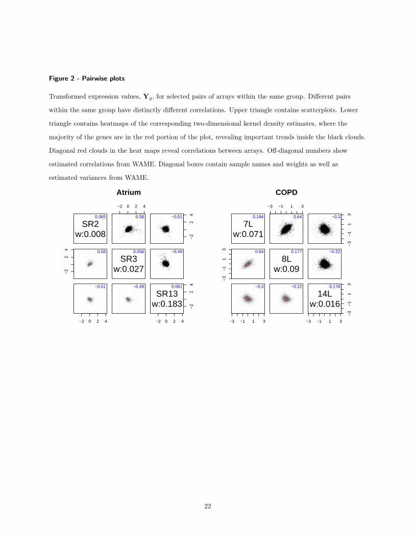
Figure 2 - Pairwise plots

Transformed expression values, Yg, for selected pairs of arrays within the same group. Different pairs

within the same group have distinctly different correlations. Upper triangle contains scatterplots. Lower

triangle contains heatmaps of the corresponding two-dimensional kernel density estimates, where the

majority of the genes are in the red portion of the plot, revealing important trends inside the black clouds.

Diagonal red clouds in the heat maps reveal correlations between arrays. Off-diagonal numbers show

estimated correlations from WAME. Diagonal boxes contain sample names and weights as well as

estimated variances from WAME.

0.065

SR2w:0.008

−2 0 2 4

0.58

−2

24−0.51

−2

24 0.58 0.056

SR3w:0.027

−0.49

−2 0 2 4

−0.51 −0.49

−2 0 2 4

−2

240.061

SR13w:0.183

Atrium

0.194

7Lw:0.071

−3 −1 1 3

0.64

−3

−1

13−0.3

−3

−1

13 0.64 0.177

8Lw:0.09

−0.22

−3 −1 1 3

−0.3 −0.22

−3 −1 1 3

−3

−1

130.178

14Lw:0.016

COPD

22

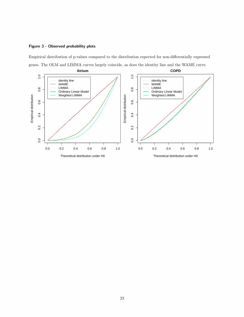
Figure 3 - Observed probability plots

Empirical distribution of p-values compared to the distribution expected for non-differentially expressed

genes. The OLM and LIMMA curves largely coincide, as does the identity line and the WAME curve.

0.0 0.2 0.4 0.6 0.8 1.0

0.0

0.2

0.4

0.6

0.8

1.0

Atrium

Theoretical distribution under H0

Em

piric

al d

istr

ibut

ion

identity lineWAMELIMMAOrdinary Linear ModelWeighted LIMMA

0.0 0.2 0.4 0.6 0.8 1.0

0.0

0.2

0.4

0.6

0.8

1.0

COPD

Theoretical distribution under H0

Em

piric

al d

istr

ibut

ion

identity lineWAMELIMMAOrdinary Linear ModelWeighted LIMMA

23

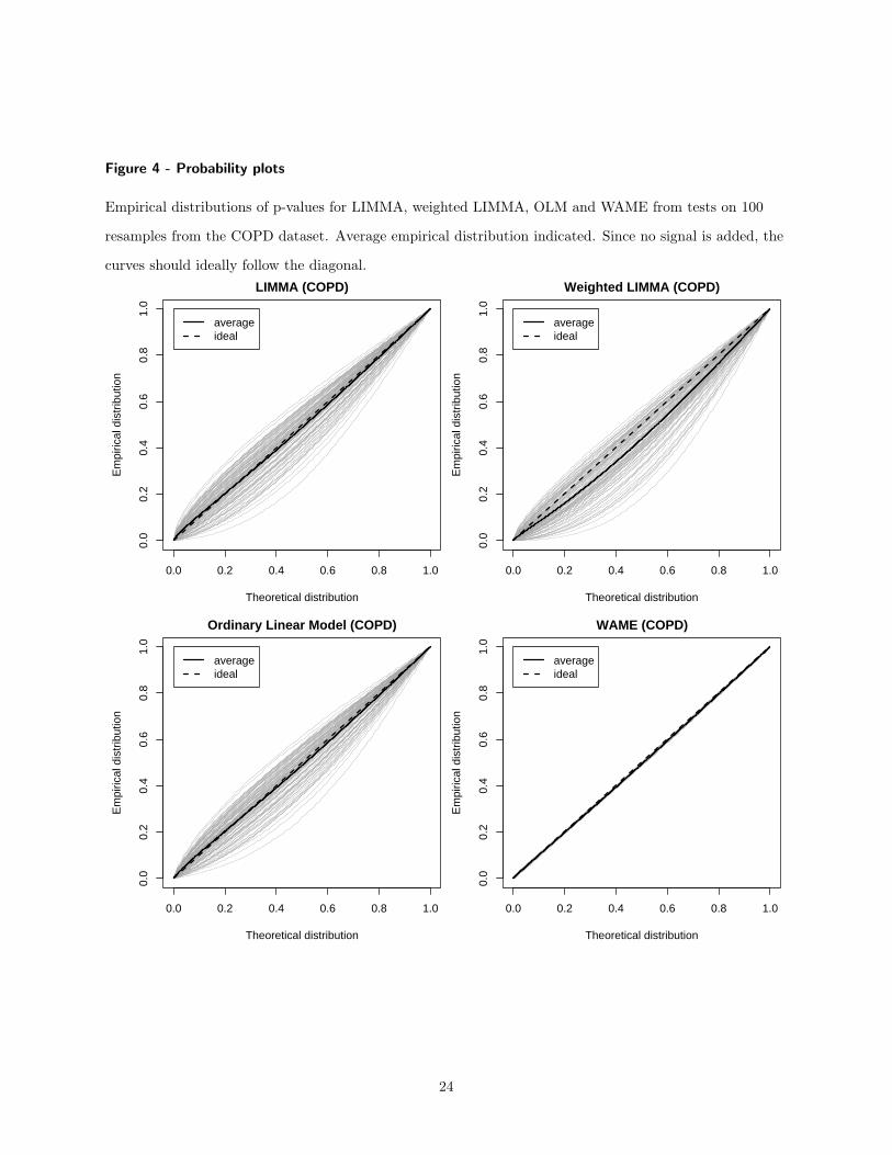
Figure 4 - Probability plots

Empirical distributions of p-values for LIMMA, weighted LIMMA, OLM and WAME from tests on 100

resamples from the COPD dataset. Average empirical distribution indicated. Since no signal is added, the

curves should ideally follow the diagonal.

0.0 0.2 0.4 0.6 0.8 1.0

0.0

0.2

0.4

0.6

0.8

1.0

LIMMA (COPD)

Theoretical distribution

Em

piric

al d

istr

ibut

ion

averageideal

0.0 0.2 0.4 0.6 0.8 1.0

0.0

0.2

0.4

0.6

0.8

1.0

Weighted LIMMA (COPD)

Theoretical distribution

Em

piric

al d

istr

ibut

ion

averageideal

0.0 0.2 0.4 0.6 0.8 1.0

0.0

0.2

0.4

0.6

0.8

1.0

Ordinary Linear Model (COPD)

Theoretical distribution

Em

piric

al d

istr

ibut

ion

averageideal

0.0 0.2 0.4 0.6 0.8 1.0

0.0

0.2

0.4

0.6

0.8

1.0

WAME (COPD)

Theoretical distribution

Em

piric

al d

istr

ibut

ion

averageideal

24

Figure 5 - Average empirical p-value distribution for WAME under regulation

Average empirical p-value distribution of the unregulated genes, calculated using WAME, when 0%, 0.1%,

1%, 5% and 10% of the genes have a log2 differential expression of 1, i.e. a two-fold change. When genes

are regulated the estimate of Σ is biased, leading to conservative, non-diagonal curves.

0.0 0.2 0.4 0.6 0.8 1.0

0.0

0.2

0.4

0.6

0.8

1.0

Atrium

Theoretical distribution

Ave

rage

em

piric

al d

istr

ibut

ion

10% d.e.5% d.e.1% d.e.0.1% d.e.0% d.e.ideal

0.0 0.2 0.4 0.6 0.8 1.0

0.0

0.2

0.4

0.6

0.8

1.0

COPD

Theoretical distribution

Ave

rage

em

piric

al d

istr

ibut

ion

10% d.e.5% d.e.1% d.e.0.1% d.e.0% d.e.ideal

25

Figure 6 - Estimated power

Estimated power in the simulated data for level 0.1% tests, based on resamples from the respective larger

group in the Atrium and COPD datasets. Power is estimated at the marked points and spline interpolation

is used in between.

1.0 1.5 2.0 2.5 3.0 3.5

0.0

0.2

0.4

0.6

0.8

1.0

Atrium

fold change

pow

er e

stim

ate

● ●

●

●

●

●

●

●

●●

●● ● ● ● ●

● WAMELIMMAwLIMMAOLMFC

1.0 1.5 2.0 2.5 3.0 3.5

0.0

0.2

0.4

0.6

0.8

1.0

COPD

fold change

pow

er e

stim

ate

● ●●

●

●

●

●

●

●

●●

● ● ● ● ●

● WAMELIMMAwLIMMAOLMFC

26

Tables

Table 1 - WAME weights

Weights in percent from estimate of differential expression using WAME.

AtriumSinus rythm Atrial fibrillation

3.0 -0.8 -2.7 -1.9 -4.6 -0.7 14.9 8.5 21.0 12.2 10.7-9.4 1.9 -5.1 0.3 -5.2 -18.3 7.5 16.6 2.1 11.8 5.3-10.6 -8.9 -9.9 -19.8 -9.4 -20.4 6.5 5.2

COPDNo/mild emphysema Severe emphysema

-18.0 -6.7 -3.9 -8.9 11.8 2.6 12.0 4.0 12.6 7.6-10.6 -7.3 -8.0 -5.6 7.1 9.0 6.7 0.9 6.2 5.5-8.3 -3.6 -14.9 -4.3 -0.3 1.6 3.2 7.6 4.3 -2.5

Table 2 - Concordance of top lists

Number of mutually included genes in the top-100 lists as determined by the different methods.

Atrium WAME LIMMA wLIMMA OLM FCWAME 100 47 45 44 15LIMMA 47 100 80 88 26wLIMMA 45 80 100 76 21OLM 44 88 76 100 21FC 15 26 21 21 100

COPD WAME LIMMA wLIMMA OLM FCWAME 100 46 47 41 22LIMMA 46 100 77 78 35wLIMMA 47 77 100 66 32OLM 41 78 66 100 25FC 22 35 32 25 100

27

Paper 4

Evolutionary forces act on promoter length:assessment of enriched cis-regulatory motifs

Erik Kristiansson1∗, Michael Thorsen2

Markus J. Tamas2, Olle Nerman1

1 Department of Mathematical Statistics, Chalmers University of Technology, S-412 96Goteborg, Sweden.2 Department of Mathematical Statistics, Goteborg University, S-405 30, Goteborg, Swe-den.3 Department of Cell and Molecular Biology/Microbiology, Goteborg University, S-405 30Goteborg, Sweden.∗ Corresponding author, erikkr math.chalmers.se

1

Abstract

BackgroundTranscription factors regulate transcription by binding to specific DNA se-quences (cis-regulatory motifs) in the promoters of their target genes. Severalmethods for finding enrichments of such motifs within a set of genes, for ex-ample genes regulated in a microarray experiment, have been proposed. Al-though the increasing preciseness of genomic data in general improves thesemethods, they will on certain occasions perform inaccurately.

ResultsWe have found that promoter length and gene function are related. In partic-ular, there are differences in promoter length between stress responsive andunresponsive genes. Our analysis suggests that genes with complex tran-scriptional regulation tend to have longer promoters than genes respondingto fewer signals. Furthermore, this phenomenon is shown to be conserved inyeast, fungi and plants, thus evolutionary forces may act on promoter length.These new findings are utilized in a novel method for assessing enrichments ofcis-regulatory motifs in promoter regions. The procedure extends logistic re-gression and includes the promoter lengths as a critical element. Evaluationson several datasets show that the proposed method generates more accuratep-values and less false positives compared to other common procedures.

ConclusionsPromoter length is associated with gene function and genes responsive to sev-eral stimuli generally have longer promoters. A novel method for assessingenrichment of cis-regulatory motifs is introduced and is shown to generatefewer false positives for sets of genes with biases in promoter length. Foranalysis of S. cerevisiae datasets, the method is available as a web servicelocated at http://enricher.math.chalmers.se.

Background

Interactions between proteins and DNA are central in most aspects of ge-netic activity including gene transcription and DNA packaging, replicationand repair. Consequently, it is of great importance to further develop thetechnologies needed to identify and/or predict these interactions. In tran-scriptional regulation, the protein-DNA interaction consists of the bindingof a transcription factor to a specific cis-regulatory motif in the promoter

2

of its target genes, thereby regulating the recruitment of the transcriptionalmachinery. The transcriptional patterns of most genes are thus dependenton the presence of cis-regulatory motifs in their promoters. Hence, analysisof promoter sequences can aid in predicting the expression pattern of tran-scriptionally regulated genes. In a reverse approach, it is possible to examineexpression patterns and deduce transcription factors involved in the tran-scriptional regulation of genes. Typically, this is done by identification ofgenes with similar transcriptional profiles and consecutive analysis of enrich-ments of the motifs located in the promoters of these genes [1, 2]. To thisend, a number of procedures have been suggested, such as the hypergeometrictest [3-5] and several tests based on regression models [6-8].

A multitude of sensing mechanisms has evolved to monitor the intra andextra cellular environment. Changes in the physical/chemical milieu willtrigger specific sensing and signaling mechanisms allowing the cell to re-spond appropriately. In many cases, the signaling will initiate a change intranscription of relevant genes resulting in an optimised composition of thecell’s proteome. The physiological adaptation to a new environment typi-cally requires turning on or off the expression of several genes. Additionally,modulations in the expression levels of many other genes may be required.For the lower eukaryotic model organism Saccharomyces cerevisiae, manyinvestigations have shown that environmental perturbations change the ex-pression levels of up to 15-20% of the entire genome [1, 2, 9-11]. When weinvestigated the regulatory responses of the genes with altered transcriptionlevels after arsenite exposure [2], we found randomly generated motifs to beenriched compared to the other genes in the genome. Here we argue thatthis peculiar bias stems from differences in the length of the promoters.

Even in a compact genome such as that of S. cerevisiae, it is evident thatthe length of the intergenic regions varies substantially. This is a potentialpitfall that the enrichment studies described hitherto have failed to address.Still, most promoter analyses circumvent the problem by defining the pro-moter as a fixed number of base pairs (bp) upstream of the transcriptionalstart site. Typically 1000 bp is used [10, 12, 13] but both 800 bp [14, 15]and 600 bp [16] are also common. To our knowledge, no regulatory motifssituated in the coding region of a gene have been described in S. cerevisiaeand it is therefore likely that cis-regulatory elements predominately occur inthe intergenic sequence [17]. The median intergenic distance in S. cerevisiaeis 455 bp. However, since the variation in promoter length is large [18], afixed promoter length (e.g. 1000 bp) is a non-optimal solution.

In this paper we show that functional information is encoded in the pro-moter length. In particular, we identify several groups of genes with longer

3

or shorter promoters than the rest of the genes in the genome. Furthermore,we show that these differences are conserved in other yeast species and maytherefore be a result of evolutionary forces. Consequently, we propose a re-gression model to assess enrichments of cis-regulatory motifs in the promotersin a group of genes. The method takes the promoter length into account andcan thus perform satisfactory when there is a difference in promoter lengthbetween the group the remaining genes in the genome. Cis-regulatory motifenrichment studies using the proposed method can be performed with theweb service Enricher located at http://enricher.math.chalmers.se.

Results

Promoter length in Saccharomyces cerevisiae

The simplest definition of a gene’s promoter region is the DNA sequencelocated 5’ of the corresponding ORF and stretching to the upstream ORF,i.e. the entire upstream intergenic region. Extracting all promoters by thisdefinition revealed that the median length of all promoter regions in the S.cerevisiae genome is 455 bp and that the length of promoters varies greatly(Figure 1).

Promoter length differs between subsets of functionally relatedgenes

By analyzing biologically meaningful gene sets, we wanted to explore if func-tional information can be extracted from promoter lengths. In two recentgenomic studies in S. cerevisiae, a large set of genes has been identified asdifferentially expressed in response to a variety of environmental perturba-tions. This phenomenon was called the environmental stress response (ESR)comprising 800 genes [10] or the common environmental response (CER)comprising 600 genes [9]. The ESR and the CER gene sets are largely over-lapping and the genes respond similarly in response to environmental stimuli,including temperature shock, osmotic stress, oxidative stress, low pH, highpH, and nutrient starvation. Our analyses show that the ESR and CERgenes have relatively long promoters. The median promoter length of ESRgenes is 493 bp which should be compared to the median length of the un-responsive genes of 450 bp (p = 2 × 10−3). Similarly, the median promoterlength of CER genes is 552 bp compared to 445 bp for the promoters of theremaining genes (p = 5 × 10−11) (Table 1 and Figure 2). The low p-valuesimply a statistically significant bias towards longer promoters for genes of

4

the environmental stress response compared to other genes (see Materialsand Methods for a description of the testing procedure).

We went on to look for other categories of genes that differ in promoterlength as compared to the rest of the genes in the genome. Interestingly, thepromoters of several classes of genes were found to have significantly longeror shorter promoters (Table 1). According to the Saccharomyces GenomeDatabase (SGD) [19], 1033 genes are essential for growth in rich medium.Our analysis revealed that these genes have very short promoters. The me-dian promoter length for the essential genes is 385 bp whereas the medianpromoter length for non-essential genes is 468 bp (p = 8 × 10−9). Investi-gating whether functional classes of genes differ in their promoter lengths,e.g. genes annotated similarly in the Yeast GO Slim terms [20], we foundthat most functional classes do not exhibit biases. However, certain classessuch as cell wall (median length 899 bp, p = 2× 10−11), transporter activity(median length 583 bp, p = 4 × 10−9) and RNA metabolic process (medianlength 340 bp, p = 6× 10−9) do differ significantly in their promoter lengths.Lists of all GO Slim terms and their corresponding promoter lengths areavailable as supplementary information (Supplementary Table 1).

Relatively long promoters of stress regulated genes may be a con-served phenomenon

To investigate if the relationship between promoter length and gene func-tion is an evolutionary conserved feature, we extended our analysis to in-clude other species. The filamentous fungus Ashbya gossypii has the smallestgenome of any free-living eukaryote reported so far. The genome is extremelycompact with a median distance between open reading frames of only 342base pairs. A. gossypii and S. cerevisiae diverged more than 100 million yearsago, and their genomes differ substantially in GC content. Still, 95% of theprotein-coding sequences of A. gossypii have homologues in the S. cerevisiaegenome with the vast majority at syntenic locations [21]. Therefore we couldeasily find 405 of the homologous genes from the common environmentalstress response in S. cerevisiae in the A. gossypii genome. We find that theseputative CER genes in A. gossypii have a median promoter length of 407 bp,which is significantly longer than the median promoter length of remaininggenes of 337 bp (p = 4 × 10−5) (Table 1). When we look at A. gossypiihomologues of the genes essential in S. cerevisiae we find the promoters tobe much shorter than the promoters of non-essential genes (p = 4 × 10−9).These differences may be a consequence of evolutionary constraints but canalso be explained as an indirect effect of the high degree of synteny between

5

the species.The evolutionary divergence between the fission yeast Schizosaccharomyces

pombe and the budding yeast S. cerevisiae is estimated to 1,14 billion years[22], approximately equal to the distance between S. cerevisiae and man.Therefore, an analysis of the promoters in the S. pombe genome could bea better indication for any potential evolutionary constraints on promoterlength. We extracted the promoters of the S. pombe genome similarly to ourS. cerevisiae approach. The median length of the promoter regions in the S.pombe genome is 829 bp and the length of promoters varies greatly (Supple-mentary Figure 1). Similar to S. cerevisiae, the environmental stress responseof S. pombe has been reported. Analyses of the S. pombe transcriptome re-vealed that many genes display analogous transcriptional profiles in responseto oxidative stress, cadmium stress, temperature shock, osmotic stress, andto a DNA damaging agent. Here, the authors named it the core environ-mental stress response (CESR) [23]. A conservative definition of the CESRcomprises 237 genes whereas a more loose definition resulted in 704 genes.The conservative definition of the CESR is genes that are induced more thantwo fold in at least four of the five conditions tested. The loose definition isthe genes that were consistently induced in response to all stresses, but failedto make the twofold cutoff in some of the responses. With the loose defini-tion of CESR, the genes have a median promoter length of 863 bp, comparedto the median of the remaining promoters of 826 bp (p = 2 × 10−2). How-ever, analyzing the genes of the conservatively defined CESR gives a morestriking result. Here, the median length of the regulated genes is 1243 bpwhile the median length of the unregulated genes is 816 bp (p = 7 × 10−15)(Supplementary Figure 2).

Next, we analyzed promoter lengths in the genome of the plant Arabidop-sis thaliana. Identification of genes transcriptionally up-regulated in responseto environmental stress treatments (heat, cold, drought, salt, high osmolar-ity, UV-B light and wounding) has been reported [24]. When performing thesame promoter analysis as above, we found that the median promoter lengthfor A. thaliana environmental stress responsive genes were 1672 bp comparedto the 1113 bp of the promoters of the remaining genes (p¡10-16) (Table 1).Taken together our findings suggest that evolutionary forces act on promoterlength.

Correlation between promoter length and cis-regulatory motifs

The examples presented above warrant for caution when trying to assessenrichment of cis-regulatory motifs in promoter sequences. Naturally, the

6

likelihood of a random occurrence of any motif increases with the promoterlength as, illustrated in Figure 3 (dotted line). In this figure, the numberof different cis-regulatory motifs and the promoter length are shown for allgenes in the genome of S. cerevisiae. A higher number of different motifs inlonger promoters is also observed when the noise level is reduced by phylo-genetic filtering (Figure 3, solid line) and may thus be a biologically relevantphenomenon.

In a reversed approach, we analysed the transcriptional profiles of thegenes in the CER and divided all genes into classes depending on the num-ber of stress conditions to which they respond. Plotting the median promoterlength of each group against the number of stress conditions, a highly pos-itive trend (p-value ¡ 10-5) and a good correlation (r2=0.96, p = 1 × 10−3)is observed (Figure 4). The same was done for the Arabidopsis promotersand again we found a positive trend between the promoter length and thenumber of different conditions which induces transcription of the gene (Sup-plementary Figure 3). This indicates that the length of promoters correlateswith the number of signals that is integrated onto the promoters.

Assessing enrichment of cis-regulatory motifs under promoter lengthbias

Procedures for finding enrichments of cis-regulatory motifs are today wellestablished tools in many aspects of modern biology. These methods areapplied to a set of genes, typically from a microarray or chromatin immuno-precipitation assay, but other assortments are also possible.

One of the most frequently used methods to find overrepresented motifsis the hypergeometric test (also known as Fishers exact test) [3, 4, 25]. Fora given set of genes, the hypergeometric test is performed by observing thenumber of genes in the set that has the motif present. Under the assumptionof independence, this number has a known distribution and hence significancecan be derived. Various kinds of regression models have also been suggestedfor identification of enriched motifs [6, 26]. In particular, logistic regression,where the presence of the motif and the selection of a gene is considered to bebinary variables (i.e. present or not, selected or not), is commonly used [7, 8].In contrast to the hypergeometric test, significance in the regression modelsis derived by large sample approximations and they are thus not suitable forsets with very few genes.

Their popularity notwithstanding, both the hypergeometric test and thelogistic regression model assume, directly or indirectly, that there is no dif-ference in promoter length between the sets of genes. We therefore propose a

7

novel procedure to assess enrichments of cis-regulatory motifs in the promot-ers of a set of genes. The method includes the promoter lengths as covariatesand can thus handle length biases in a proper manner. The model is basedon the generalized additive model (GAM) framework [27, 28] and can be seenas an extension of logistic regression. Further details for all three methodsdiscussed here can be found in Materials and Methods.

Promoter length bias can result in false positives

A simulation study was performed to compare the proposed model to the hy-pergeometric test and logistic regression. Datasets, divided into two groupsof artificial promoters, each consisting of 500 and 5000 promoters respec-tively, were generated as follows. The length of the promoters were sampledfrom uniform distributions such that the promoters in the first group were,on average, 25% longer than the promoters in the second group (median pro-moter length were 500 bp and 400 bp respectively). Given the length, eachpromoter was generated by sampling the four nucleotides with equal prob-abilities. In total, 1000 datasets were created. Further details are availablein Materials and Methods. The simulated promoters were searched for asix nucleotide long motif and tests for enrichments within the smaller groupwere performed for all three methods. Histograms of the resulting p-valuesare shown in Figure 5. Since the promoter sequences are completely random,no enrichments should exist and the p-values should therefore be uniformlydistributed between 0 and 1. The results from both the hypergeometric testand logistic regression are clearly skewed towards lower p-values. However,this is not the case for the proposed model, which suggests that it results inless false positives when there is a bias in promoter length.

Transcription factors in arsenic stress

To evaluate our model on real biological data, we assessed enrichments ofcis-regulatory elements in a microarray dataset on transcriptional changes inresponse to arsenite exposure [2]. Based on this experiment, putatively up-and down-regulated genes with an absolute log2 fold-change greater than 2where chosen for enrichment analysis. The promoter lengths of these geneswere significantly longer than the promoters in the rest of the genome (Table1). Accordingly, the model proposed in this paper is suitable for a properanalysis of this data.

Enrichment analysis of all experimentally verified cis-regulatory motifsdescribed in SGD [19] were performed. Phylogenetic filtering was used to re-

8

move spurious motifs (see Materials and Methods). Examples of significantmotifs according to the proposed model can be seen in Table 2 together withp-values from the hypergeometric test and logistic regression. In general,the p-values for highly significant motifs seem to be lower for the regressionbased methods for than the hypergeometric test. Furthermore, the proposedmethod is, as expected, more conservative than logistic regression. The lasttwo rows in Table 2 show examples of motifs that, according to the pro-posed models, are candidate false positives. These motifs have low p-valuesfor both the hypergeometric test and the logistic regression model but getsubstantially higher p-values when the promoter length is included. Com-plete lists with p-values for all cis-regulatory motifs in yeast can be found inSupplementary Table 2 and 3.

Discussion

Using the S. cerevisiae genome as a model, we analysed the length of pro-moter regions of genes in different datasets and we found a striking rela-tionship between long promoters and responsiveness to a variety of stresses.Complementary to this, we analyzed analogous datasets of promoters in S.pombe and A. thaliana found the same relationship. Thus, longer promotersof stress inducible genes seem to be a conserved phenomenon. The simplestexplanations may be that relatively long promoters allow for integration ofa large number of regulatory inputs onto the promoter region of these genesand, conversely, that other promoters may have been shortened to reducegenome size.

The integration of many signals into a promoter requires a number ofmotifs. If several signalling pathways target the same promoter, binding sitesmust exist for all relevant transcription factors. Additionally, the regulationcan be combinatorial and thus a number of auxiliary factors may also bind.In these cases, the promoters must be long enough or steric hindrances mayprevent the binding of all the necessary factors. We speculate that the levelof complexity of the regulation of a gene is related to the function of thegene product. Hence, promoters of certain classes of genes may have evolvedto be longer due to complex regulation, whereas other classes of genes mayhave evolved shorter promoters to reduce genome size. A smaller genomeis believed to be an advantage as replication is faster, allowing for fasterproliferation.

Evolution may not have acted to reduce the intergenic stretches of allgenomes. Therefore, a relationship between promoter length and regula-

9

tory complexity might not always exist. We have argued here that utilis-ing the information about the length of the individual promoters improvesthe validity of the p-values generated when estimating enrichments of cis-regulatory motifs in S. cerevisiae and S. pombe datasets. Similar analy-ses of mammalian promoters may be difficult, as they in general are muchlonger and poorly defined. However, the annotation of mammalian genomesis improving and several resources for extracting promoter sequences frommammalian genomes exist. One interesting study on the organisation of thehuman genome clearly demonstrates that both the introns and the intergenicspace around housekeeping genes are shorter than corresponding sequencesfor tissue specific genes. Similar tendencies are also reported for the flyDrosophila melanogaster and the worm Caenorhabditis elegans. The authorspeculated that the tissue specific genes have a more composite transcrip-tional regulation, and thus require longer sequences to facilitate a more dy-namic chromatin structure [29]. These findings corroborate our conclusionsand indicate that promoter length is an important factor when analysinggenomes of higher eukaryotes.

Assessing enrichments of de novo motifs is a process where the rate offalse positives has been particularly bothersome. A recent report [30] iden-tified a number of problems which needs to be addressed to improve thesemethods. Among them were: (I) the lack of rigorous models and of an exactp-value measuring motif enrichment; (II) the tendency, in many of the exist-ing methods, to report presumably significant motifs even when applied torandomly generated data. We believe that our model is a novel approach to(I) and a clear improvement of (II).

Our model may also be of use in other types of enrichment studies. Inpost-transcriptional regulation, RNA binding proteins (RBPs) interact withsites in the untranslated regions (UTRs) of the mRNAs and regulate local-ization, degradation, and translational control. In S. cerevisiae, the lengthof the UTRs has been shown to depend on gene function [31] and the num-ber of identified RBP binding motifs is increasing [32]. Hence, biases in UTRlengths between groups of genes cannot be ruled out, and the proposed modelshould be straight-forward to apply in these situations.

Eukaryotic genomes are packaged into nucleosome particles that preventthe DNA from interacting with other DNA binding proteins. Experimentalevidence shows that DNA packaging can control accessibility of specific se-quences by blocking access to irrelevant non-functional sites [33, 34]. A futuredirection would therefore be to incorporate chromatin structure predictioninto the enrichment analysis. A computational method modelling nucleosomepositioning has recently been developed, that can predict roughly 50% of the

10

genome-wide nucleosome organisation in yeast [35]. Additional informationcan be extracted by predict acetylation and methylation of nucleosomes toidentify sequences with regulatory activity [36]. These are important areasof research and further development of these tools is needed to improve theiraccuracy. Combining robust prediction algorithms for nucleosome organisa-tion with phylogenetic based comparative genomics holds great promises forvastly enhanced prediction of true cis-regulatory elements.

Conclusion

We have presented evidence that promoter lengths include functional infor-mation and several categories of genes have been shown to have promoterslonger or shorter than promoters of the other genes in the genome. This wasseen for stress induced genes in S. cerevisiae, A. gossypii, S. pombe and A.thaliana thus evolutionary forces may act on promoter length. Consequently,we have developed a method for assessing enrichments of cis-regulatory mo-tifs in sets of promoters with varying lengths. To our knowledge, this is thefirst model which utilizes information encoded in the promoter lengths to findoverrepresentations of transcription factor binding sites. Simulations showthat the proposed model performs adequately, in contrast to the hypergeo-metric test and logistic regression, which both can lead to false positives.

Materials and Methods

Sequence data and analysis

The intergenic regions for both Saccharomyces cerevisiae and Schizosaccha-romyces pombe were downloaded from the GeneDB database [37] (March,2007). For each gene, the 5’ upstream sequence from the start of the openreading frame (ORF) until the end of the previous ORF (on any strand)was extracted. In this study, these sequences are referred to as promoters.Genes with ORFs overlapping other genes such that the intergenic region isnonexistent were removed from the analysis. This resulted in 5735 promotersin S. cerevisiae and 5484 promoters in S. pombe. Sequence data for Saccha-romyces mikatae, Saccharomyces kudriavzevii, Saccharomyces bayanus, Sac-charomyces castellii, and Saccharomyces kluyveri, all yeast species closelyrelated to S. cerevisiae [38], were downloaded from SGD [19] (April, 2007).Intergenic regions for every gene with a homologue in S. cerevisiae wereextracted and cut at the same position as the corresponding promoter in

11

S. cerevisiae, resulting in 2983, 3606, 4733, 4090 and 2798 promoters for S.mikatae, S. kudriavzevii, S. bayanus, S. castellii, and S. kluyveri, respectively.Intergenic regions for A. gossypii were extracted from the Ashyba GenomeDatabase (AGD) [39] and S. cerevisiae homologues were mapped using thetable published in Dietrich et al. 2004 [21]. Intergenic regions for A. thalianawere retrieved from the TAIR database [40]. The total number of promotersfor A. gossypii and A. thaliana were 4683 and 27736 respectively.

All tests of differences in promoter lengths between groups of genes per-formed in this study were done using the Wilcoxon rank sum test. This is anon-parametric procedure designed to test differences between medians andis therefore robust against exaggerated promoter lengths.

Transcription factor binding site data and phylogenetic filtering

129 known transcription factor binding sites (motifs), corresponding to 92distinct transcription factors in S. cerevisiae, were downloaded from SGD(March, 2007). The motifs were described by IUPAC-codes. The length ofthe motifs varied between 5 bp and 20 bp (9 bp in average). A motif wasdefined as present in a promoter in S. cerevisiae given at least one exactmatch. Under phylogenetic filtering, a motif was defined as present if it was(1) present in the promoter of S. cerevisiae and (2) present in at least halfof the available corresponding promoters in the closely related species. Notethat the position of a motif can vary in the promoters between the differentspecies.

Mathematical details and model descriptions

Assume that there are N genes in the genome and that we are interested intesting overrepresentation of a motif within a subset A consisting of n genes.For g = 1, . . . , N , let xg be a binary 0,1 valued variable indicating whetherthe motif is present in the promoter of gene g. Furthermore let yg be anotherbinary variable indicating if gene g belongs to the subset A. Let zg = xgyg

, i.e. zg is one if gene g is in the subset A and has the motif present in thepromoter. Finally, let lg be the length of the promoter for gene g.

The hypergeometric test can be seen as drawing a fixed number of balls(genes in A) from an urn consisting of red (genes with a motif) and blue(genes without a motif) balls. The observed number of red balls among thedrawn balls (genes in A with the motif) can then be compared to all otherpossible draws and the significance calculated. If we let xtot =

∑xg and

12

ztot =∑

zg , then

phyper =

min(xg ,n)∑i=ztot

(xtot

i

) (N − xtot

n− i

)(

Nn

) .

The hypergeometric test relies on the assumption that all balls are drawnwith equal probability, i.e., that motifs occur with the same probability inall promoters, which is questionable if there is a bias in promoter length.

The standard logistic regression model can be formulated as a linear re-lationship between the log-odds of having the motif present (yg) and theselection of the gene (xg), i.e.

logP(yg = 1)

P(yg = 0)= α + βxg.

The coefficients α and β are estimated from data and an enrichment can beinferred by testing whether β is positive. Note that under the null hypothesis,i.e., when β is zero, the probability of finding the motif is equal for all genesregardless of the length of the promoter.

The method proposed in this paper is an extension of the logistic regres-sion model to a generalized additive model (GAM) [27, 28, 41]. In GAMs,non-linear relations of covariates are modelled non-parametric by smoothingfunctions. In our case, an unknown function of the promoter length is addedto compensate for any bias in the set of genes of interest. In other words,we assume that the log-odds of the presence of the motif depends both onthe selection of the gene and the length of the promoter. Using the samenotation as above, the extended model can be formulated as

logP(yg = 1)

P(yg = 0)= α + βxg + f(lg),

where f is an unknown smooth function. The coefficients α and β and thefunction f are estimated from data. Extremely long promoters, typicallycoming for regions scarce of ORFs such as the telomeres, were truncated atthe 95th percentile resulting in a maximal length of 1902 bp. A p-value foroverrepresentation can then, as for the logistic regression model, be calculatedby testing whether β is positive.

All calculations were performed using the statistical language R [42]. Themgcv package [28] was used to fit the GAM. For the logistic regression model,

13

the maximum likelihood estimates of the coefficients α and β were found us-ing iterated re-weighted least squared (IRLS). A penalized version of IRLS(P-IRLS) was used, together with the UBRE smoothing condition, to es-timate the function f and the coefficients α and β for the generalized ad-ditive model. For both models, overrepresentation was inferred by testingH0 : β = 0 versus HA : β > 0. Large sample normal approximations ofthe estimated values of β were used to calculate p-values. Enrichments ofmotifs with less than 5 hits within the gene set A were not performed by theregression models. Further details regarding the GAMs are available in [28].

Details regarding the simulation study

The data for the simulation study was generated as follows. Two sets ofartificial promoters were created, one with 500 and the other with 5000 se-quences. The length of the promoters in the first group was chosen uniformlybetween 1 and 1000 and the corresponding distribution for the second groupwas uniform between 1 and 900. The average length difference thus becomes100 bp, which is typical for the different microarray datasets examined inthis study. Given the length, the nucleotide sequence of the promoters wasgenerated by repeatedly sampling from A, C, G, and T with equal proba-bility. In total, 1000 such sets of promoters were generated (i.e. 1000 setswere each set has 5500 promoters in total) and for each set enrichment of asix-nucleotide motif was inferred.

Authors’ contributions

The analyses were designed by EK and MT and performed by EK in collab-oration with ON. The proposed model was formulated by EK and ON. Themanuscript was drafted by EK and MT and read, edited and approved byall authors.

Acknowledgement

This research was financed by the Swedish National Research School in Ge-nomics and Bioinformatics. We also would like to thank Alexandra Jauhi-ainen for extensive comments and suggestions on the manuscript and JonasWaringer and Olga Kourtchenko for discussions.

14

References

[1] Boer VM, de Winde JH, Pronk JT, Piper MD: The genome-wide tran-scriptional responses of Saccharomyces cerevisiae grown on glucose inaerobic chemostat cultures limited for carbon, nitrogen, phosphorus, orsulfur. J Biol Chem 2003, 278(5):3265-3274.

[2] Thorsen M, Lagniel G, Kristiansson E, Junot C, Nerman O, Labarre J,Tamas MJ: Quantitative transcriptome, proteome and sulfur metaboliteprofiling of the Saccharomyces cerevisiae response to arsenite. PhysiolGenomics 2007.

[3] Hughes JD, Estep PW, Tavazoie S, Church GM: Computational identi-fication of cis-regulatory elements associated with groups of functionallyrelated genes in Saccharomyces cerevisiae. J Mol Biol 2000, 296(5):1205-1214.

[4] Sharan R, Ovcharenko I, Ben-Hur A, Karp RM: CREME: a frameworkfor identifying cis-regulatory modules in human-mouse conserved seg-ments. Bioinformatics 2003, 19 Suppl 1:i283-291.

[5] Ettwiller L, Paten B, Souren M, Loosli F, Wittbrodt J, Birney E: Thediscovery, positioning and verification of a set of transcription-associatedmotifs in vertebrates. Genome Biol 2005, 6(12):R104.

[6] Bussemaker HJ, Li H, Siggia ED: Regulatory element detection usingcorrelation with expression. Nat Genet 2001, 27(2):167-171.

[7] Copley RR: The EH1 motif in metazoan transcription factors. BMCGenomics 2005, 6:169.

[8] Keles S, van der Laan MJ, Vulpe C: Regulatory motif finding by logicregression. Bioinformatics 2004, 20(16):2799-2811.

[9] Causton HC, Ren B, Koh SS, Harbison CT, Kanin E, Jennings EG,Lee TI, True HL, Lander ES, Young RA: Remodeling of yeast genomeexpression in response to environmental changes. Mol Biol Cell 2001,12(2):323-337.

[10] Gasch AP, Spellman PT, Kao CM, Carmel-Harel O, Eisen MB, Storz G,Botstein D, Brown PO: Genomic expression programs in the response ofyeast cells to environmental changes. Mol Biol Cell 2000, 11(12):4241-4257.

15

[11] Lai LC, Kosorukoff AL, Burke PV, Kwast KE: Dynamical remodelingof the transcriptome during short-term anaerobiosis in Saccharomycescerevisiae: differential response and role of Msn2 and/or Msn4 and otherfactors in galactose and glucose media. Mol Cell Biol 2005, 25(10):4075-4091.

[12] Haverty PM, Hansen U, Weng Z: Computational inference of transcrip-tional regulatory networks from expression profiling and transcriptionfactor binding site identification. Nucleic Acids Res 2004, 32(1):179-188.

[13] Liu Y, Ringner M: Revealing signaling pathway deregulation by usinggene expression signatures and regulatory motif analysis. Genome Biol2007, 8(5):R77.

[14] Daran-Lapujade P, Jansen ML, Daran JM, van Gulik W, de WindeJH, Pronk JT: Role of transcriptional regulation in controlling fluxesin central carbon metabolism of Saccharomyces cerevisiae. A chemostatculture study. J Biol Chem 2004, 279(10):9125-9138.

[15] Garcia R, Bermejo C, Grau C, Perez R, Rodriguez-Pena JM, Francois J,Nombela C, Arroyo J: The global transcriptional response to transientcell wall damage in Saccharomyces cerevisiae and its regulation by thecell integrity signaling pathway. J Biol Chem 2004, 279(15):15183-15195.

[16] Patil CK, Li H, Walter P: Gcn4p and novel upstream activating se-quences regulate targets of the unfolded protein response. PLoS Biol2004, 2(8):E246.

[17] Gasch AP, Moses AM, Chiang DY, Fraser HB, Berardini M, EisenMB: Conservation and evolution of cis-regulatory systems in ascomycetefungi. PLoS Biol 2004, 2(12):e398.

[18] Wood V, Gwilliam R, Rajandream MA, Lyne M, Lyne R, Stewart A,Sgouros J, Peat N, Hayles J, Baker S et al: The genome sequence ofSchizosaccharomyces pombe. Nature 2002, 415(6874):871-880.

[19] Cherry JM, Ball C, Weng S, Juvik G, Schmidt R, Adler C, Dunn B,Dwight S, Riles L, Mortimer RK et al: Genetic and physical maps ofSaccharomyces cerevisiae. Nature 1997, 387(6632 Suppl):67-73.

[20] Ashburner M, Ball CA, Blake JA, Botstein D, Butler H, Cherry JM,Davis AP, Dolinski K, Dwight SS, Eppig JT et al: Gene ontology: tool

16

for the unification of biology. The Gene Ontology Consortium. Nat Genet2000, 25(1):25-29.

[21] Dietrich FS, Voegeli S, Brachat S, Lerch A, Gates K, Steiner S, Mohr C,Pohlmann R, Luedi P, Choi S et al: The Ashbya gossypii genome as atool for mapping the ancient Saccharomyces cerevisiae genome. Science2004, 304(5668):304-307.

[22] Hedges SB: The origin and evolution of model organisms. Nat Rev Genet2002, 3(11):838-849.

[23] Chen D, Toone WM, Mata J, Lyne R, Burns G, Kivinen K, Brazma A,Jones N, Bahler J: Global transcriptional responses of fission yeast toenvironmental stress. Mol Biol Cell 2003, 14(1):214-229.

[24] Kilian J, Whitehead D, Horak J, Wanke D, Weinl S, Batistic O,D’Angelo C, Bornberg-Bauer E, Kudla J, Harter K: The AtGenExpressglobal stress expression data set: protocols, evaluation and model dataanalysis of UV-B light, drought and cold stress responses. Plant J 2007,50(2):347-363.

[25] Nelander S, Larsson E, Kristiansson E, Mansson R, Nerman O, Sig-vardsson M, Mostad P, Lindahl P: Predictive screening for regulators ofconserved functional gene modules (gene batteries) in mammals. BMCGenomics 2005, 6(1):68.

[26] Boulesteix AL, Strimmer K: Predicting transcription factor activitiesfrom combined analysis of microarray and ChIP data: a partial leastsquares approach. Theor Biol Med Model 2005, 2:23.

[27] Hastie TJ, Tibshirani RJ: Generalized additive models. London: Chap-man and Hall; 1990.

[28] Wood SN: Generalized Additive Models: Chapman & Hall; 2006.

[29] Vinogradov AE: Compactness of human housekeeping genes: selectionfor economy or genomic design? Trends Genet 2004, 20(5):248-253.

[30] Eden E, Lipson D, Yogev S, Yakhini Z: Discovering motifs in rankedlists of DNA sequences. PLoS Comput Biol 2007, 3(3):e39.

17

[31] David L, Huber W, Granovskaia M, Toedling J, Palm CJ, Bofkin L,Jones T, Davis RW, Steinmetz LM: A high-resolution map of transcrip-tion in the yeast genome. Proc Natl Acad Sci U S A 2006, 103(14):5320-5325.

[32] Gerber AP, Herschlag D, Brown PO: Extensive association of function-ally and cytotopically related mRNAs with Puf family RNA-bindingproteins in yeast. PLoS Biol 2004, 2(3):E79.

[33] Sekinger EA, Moqtaderi Z, Struhl K: Intrinsic histone-DNA interactionsand low nucleosome density are important for preferential accessibilityof promoter regions in yeast. Mol Cell 2005, 18(6):735-748.

[34] Yuan GC, Liu YJ, Dion MF, Slack MD, Wu LF, Altschuler SJ, RandoOJ: Genome-scale identification of nucleosome positions in S. cerevisiae.Science 2005, 309(5734):626-630.

[35] Segal E, Fondufe-Mittendorf Y, Chen L, Thastrom A, Field Y, MooreIK, Wang JP, Widom J: A genomic code for nucleosome positioning.Nature 2006, 442(7104):772-778.

[36] Heintzman ND, Stuart RK, Hon G, Fu Y, Ching CW, Hawkins RD,Barrera LO, Van Calcar S, Qu C, Ching KA et al: Distinct and predic-tive chromatin signatures of transcriptional promoters and enhancers inthe human genome. Nat Genet 2007, 39(3):311-318.

[37] Hertz-Fowler C, Peacock CS, Wood V, Aslett M, Kerhornou A, MooneyP, Tivey A, Berriman M, Hall N, Rutherford K et al: GeneDB: a re-source for prokaryotic and eukaryotic organisms. Nucleic Acids Res 2004,32(Database issue):D339-343.

[38] Cliften P, Sudarsanam P, Desikan A, Fulton L, Fulton B, Majors J,Waterston R, Cohen BA, Johnston M: Finding functional features inSaccharomyces genomes by phylogenetic footprinting. Science 2003,301(5629):71-76.

[39] Gattiker A, Rischatsch R, Demougin P, Voegeli S, Dietrich FS,Philippsen P, Primig M: Ashbya Genome Database 3.0: a cross-speciesgenome and transcriptome browser for yeast biologists. BMC Genomics2007, 8:9.

[40] Rhee SY, Beavis W, Berardini TZ, Chen G, Dixon D, Doyle A, Garcia-Hernandez M, Huala E, Lander G, Montoya M et al: The Arabidopsis

18

Information Resource (TAIR): a model organism database providing acentralized, curated gateway to Arabidopsis biology, research materialsand community. Nucleic Acids Res 2003, 31(1):224-228.

[41] Hastie T.J T, R.J: Generalized Additive Models: Some Applications. JAm Stat Assoc 1987, 82(398):371-386.

[42] R: A Language and Environment for Statistical Computing[http://www.R-project.org]

19

Gene subset Nr. of Median Nr. of remaining Median P-valuegenes length genes length

Saccharomyces cerevisiaeGasch ESR genes 820 493 4915 450 2× 10−3

Causton CER genes 588 552 5147 445 5× 10−11

Thorsen up-regulated 317 560 5418 450 1× 10−7

Thorsen down-regulated 398 561 5337 448 3× 10−7

Essential genesa 1033 385 4702 468 8× 10−9

Ribosomal genes 185 551 5550 453 9× 10−3

Cell wall 69 899 5666 453 2× 10−11

Transporter activity 361 583 5374 449 4× 10−9

RNA metabolic process 262 340 5473 461 6× 10−9

Ashbya gossypiiCauston CER genesb 405 407 4278 337 4× 10−5

Essential genesb 1018 298 3665 356 4× 10−9

Schizosaccharomyces pombeChen CESR genes 704 863 4780 826 2× 10−2

Chen CERSconservative genes 237 1243 5247 816 7× 10−15

Arabidopsis thalianaKilian stress genesc 1152 1672 26584 1113 < 10−16

aFor growth in rich medium.bHomologues based on the map in Dietrich et al. 2004 [21].cGenes from the environmental stress microarray data in Kilian et al. 2004 [24] with anlog fold-change more than 5 in at least one condition.

Table 1: Examples of gene sets from four different species with a significantdifference in promoter length. Stress associated genes tend to have longerpromoters than other genes, while promoters of essential genes are shorter.GO categories such as cell wall, transporter activity, and RNA metabolicprocess also have a different promoter length compared to the rest of thegenes in the genome.

20

Transcription Binding site Hypergeometric Logistic Proposedfactor test regression modelRPN4 GGTGGCAAA 6× 10−19 8× 10−24 6× 10−22

YAP2 MTTASTMAKC 5× 10−12 8× 10−15 1× 10−12

YAP7 MTKASTMA 6× 10−12 2× 10−13 4× 10−9

YAP1 TTAGTMAGC 3× 10−8 1× 10−9 3× 10−8

MSN2/4 AAGGGG 3× 10−10 3× 10−11 1× 10−7

YAP2/3/4/5 TTACTAA 3× 10−9 1× 10−10 1× 10−7

YAP1 TTASTMA 6× 10−10 8× 10−10 5× 10−7

MET31/32 AAACTGTGG 6× 10−6 1× 10−6 1× 10−5

SWI5 KGCTGR 6× 10−6 6× 10−6 2× 10−2

YOX1 YAATTA 9× 10−5 1× 10−4 1× 10−1

Table 2: The upper part of the table shows the top enriched transcriptionfactors for up-regulated genes in the arsenite microarray dataset accordingto the proposed model. The median promoter length of the regulated geneswas more than 100 bp longer than the promoter length of the other genes.As predicted by the simulation study, the p-values for the hypergeometrictest and the logistic regression are non-conservative relative to the proposedmethod. The bottom part shows two examples of transcription factors havingsubstantially low- to non-significant p-values when the proposed model isused.

21

Promoter length

Fre

quen

cy

030

060

0

0 median=455 1000 2000

Figure 1: Histogram of the 5735 Saccharomyces cerevisiae promoters usedin this study. The median promoter length is 455 bp and the distribution isasymmetric with a right tail. Roughly 5% of the promoters are longer than2000 bp and thus not shown in this figure.

22

Promoter length

Den

sity

Median CER genes

Median remaining genes

0.00

00.

001

0.00

2

0 445 552 1000 2000

CER genesRemaining genes

Figure 2: Estimated densities of the promoter length for the common envi-ronmental response (CER) genes (solid line) and the remaining genes (dashedline). The median length of the promoters for the CER genes was found tobe significantly longer than for the remaining genes (p = 5× 10−11).

23

Promoter length

Num

ber

of d

iffer

ent t

rans

crip

tion

fact

or b

indi

ng s

ites

0 500 1000 1500 2000

05

1015

2025

3035

40

Figure 3: This figure shows the smoothed two-dimensional distribution ofpromoter length (x-axis) and number of different transcription factor bind-ing sitesmotifs (y-axis). Higher intensity means more genes. Phylogeneticfiltering, based on five closely relates yeast species, was used to reduce thenumber of spurious motifs. The general trend is shown both with and withoutphylogenetic filtering (solid and dashed curve respectively).

24

●

●

●

●

●

●

Number of different stress types

Med

ian

prom

oter

leng

th

400

500

600

700

800

0 1 2 3 4 5

Figure 4: The number of stress conditions is correlated with the length ofthe promoter. Expression data from Causton et al. [9] were used to cate-gorize genes into groups depending on the number of stress conditions theywere regulated in (x-axis). For each group, the median promoter length wascalculated (y-axis). The dashed line is a result of a linear regression withweights proportional to the number of genes in each group (5064, 449, 93,32, 12, and 2 genes for the groups corresponding to 0 to 5 stress conditions,respectively). The trend is clearly positive (p < 10−5) and genes regulated inseveral stress conditions have in general longer promoters. The correlationcoefficient were estimated to 0.96 (p = 10−3). Both p-values were calculatedby permuting the promoters one million times while keeping the size of thegroups fixed.

25

Hypergeometric

P−value

015

30

0.00 0.25 0.50 0.75 1.00

Logistic regression

P−value

015

30

0.00 0.25 0.50 0.75 1.00

Proposed model

P−value

015

300.00 0.25 0.50 0.75 1.00

Figure 5: Results of the simulation study. Two sets of promoters with randomsequences were created. The promoter length bias between the sets wereset to 100 bp. Enrichment of a six-nucleotide motif was assessed in theset with long promoters using three different methods; hypergeometric test,logistic regression, and the proposed method. The hypergeometric test andthe logistic regression result in several significant p-values, even though thepromoters were randomly generated and no enrichment should exist. Theproposed model, however, handles the bias well and reports no false positives.

26

Paper 5

Quantitative transcriptome, proteome, and sulfur metabolite profilingof the Saccharomyces cerevisiae response to arsenite

Michael Thorsen,1 Gilles Lagniel,2 Erik Kristiansson,3 Christophe Junot,4

Olle Nerman,3 Jean Labarre,2 and Markus J. Tamas1

1Department of Cell and Molecular Biology/Microbiology, Gothenburg University, Gothenburg, Sweden;2Service de Biochimie et de Genetique Moleculaire, Departement de Biologie Joliot-Curie, Commissariata l’Energie Atomique (CEA)/Saclay, Gif-sur-Yvette, France; 3Department of Mathematical Statistics,Chalmers University of Technology, Gothenburg, Sweden; and 4Service de Pharmacologie etImmunologie, Departement de Recherche, Medicale, CEA/Saclay, Gif-sur-Yvette, France

Submitted 27 October 2006; accepted in final form 22 February 2007

Thorsen M, Lagniel G, Kristiansson E, Junot C, Nerman O,Labarre J, Tamas MJ. Quantitative transcriptome, proteome, andsulfur metabolite profiling of the Saccharomyces cerevisiae responseto arsenite. Physiol Genomics 30: 35–43, 2007. First publishedFebruary 27, 2007; doi:10.1152/physiolgenomics.00236.2006.—Ar-senic is ubiquitously present in nature, and various mechanisms haveevolved enabling cells to evade toxicity and acquire tolerance. Herein,we explored how Saccharomyces cerevisiae (budding yeast) respondto trivalent arsenic (arsenite) by quantitative transcriptome, proteome,and sulfur metabolite profiling. Arsenite exposure affected transcrip-tion of genes encoding functions related to protein biosynthesis,arsenic detoxification, oxidative stress defense, redox maintenance,and proteolytic activity. Importantly, we observed that nearly allcomponents of the sulfate assimilation and glutathione biosynthesispathways were induced at both gene and protein levels. Kineticmetabolic profiling evidenced a significant increase in the pools ofsulfur metabolites as well as elevated cellular glutathione levels.Moreover, the flux in the sulfur assimilation pathway as well as theglutathione synthesis rate strongly increased with a concomitantreduction of sulfur incorporation into proteins. By combining com-parative genomics and molecular analyses, we pinpointed transcrip-tion factors that mediate the core of the transcriptional response toarsenite. Taken together, our data reveal that arsenite-exposed cellschannel a large part of assimilated sulfur into glutathione biosynthesis,and we provide evidence that the transcriptional regulators Yap1p andMet4p control this response in concert.

DNA microarray; proteomics; glutathione

ARSENIC IS A HIGHLY TOXIC metalloid that considerably threatensthe environment and human health. The most striking exampleis the epidemic of arsenic poisoning observed in Bangladeshand West Bengal, where arsenic contaminates the drinkingwater through geological sources and thereby affects millionsof people (10, 26). Chronic arsenic exposure causes cardiovas-cular diseases, neurological disorders, and liver injury and isassociated with cancers of the skin, bladder, liver, and lung.Despite its toxicity, arsenic trioxide is currently used as a treat-ment for acute promyelocytic leukemia, and it might also beemployed against other hematological and solid cancers (7, 28).

All organisms have been exposed to toxic agents since theorigin of life, and tolerance mechanisms arose early during

evolution. The unicellular model eukaryote Saccharomycescerevisiae (budding yeast) evades arsenic toxicity by increas-ing efflux of trivalent arsenite [As(III)] through the plasmamembrane protein Acr3p (12, 38), by sequestering glutathione-conjugated As(III) in the vacuole through the ATP bindingcassette (ABC) transporter Ycf1p (12) and by reducing As(III)influx through the aquaglyceroporin Fps1p (34, 39). In addi-tion, cells may acquire tolerance by adjusting cytosolic redoxand glutathione levels in response to As(III) (31). Two AP-1-like transcription factors have been shown to be important foryeast As(III) tolerance; Yap8p controls expression of the ar-senic-specific detoxification genes ACR2 and ACR3, whereasYap1p controls transcription of genes encoding proteins withantioxidant properties. In addition, Yap1p contributes to YCF1and ACR3 control (17, 24, 40).

Sulfur assimilation is essential for all organisms. In yeast,extracellular sulfate is taken up and metabolized through thesulfate assimilation pathway where sulfide is the reduced endproduct (33). Sulfide can then either go through the methylcycle or into the cysteine/glutathione biosynthesis pathway(Fig. 1). Hence, the fate of assimilated sulfur is principallybiosynthesis of the sulfur-containing amino acids methionineand cysteine and the low-molecular-weight thiol moleculesS-adenosylmethionine and glutathione (GSH) (33). GSH is akey factor in the cell’s defense against oxidative stress andmetal toxicity. GSH may detoxify metals by 1) chelationfollowed by vacuolar sequestration; 2) protecting against oxi-dation caused by metals, since GSH serves as the main redoxbuffer of the cell; and 3) binding to reactive sulfhydryl groupson proteins (protein glutathionylation), thereby protecting themfrom irreversible metal binding and/or oxidative damage (13,27). Whether protein glutathionylation occurs in response tometals has not been investigated. Transcription of the genesencoding enzymes in the sulfate assimilation/GSH biosynthe-sis pathways is principally controlled by the transcriptionalactivator Met4p. Met4p is recruited to target promoters by theDNA binding proteins Met28p, Met31p, Met32p, and Cbf1p,forming the complexes Met4p-Met31p/Met32p and Met4p-Cbf1p-Met28p (33). Interestingly, Met4p has been shown toplay a central role in cadmium tolerance by controllingexpression of sulfur assimilation and GSH biosynthesisgenes (8).

The aim of this study was to gain detailed insight into theyeast response to arsenite. We demonstrate that As(III)-ex-posed cells channel a large part of assimilated sulfur into GSH

Article published online before print. See web site for date of publication(http://physiolgenomics.physiology.org).

Address for reprint requests and other correspondence: M. J. Tamas, Dept.of Cell and Molecular Biology/Microbiology, Goteborg Univ., S-405 30Goteborg, Sweden (e-mail: markus.tamas@gmm.gu.se).

Physiol Genomics 30: 35–43, 2007.First published February 27, 2007; doi:10.1152/physiolgenomics.00236.2006.

1094-8341/07 $8.00 Copyright © 2007 the American Physiological Society 35

on June 20, 2007 physiolgenom

ics.physiology.orgD

ownloaded from

biosynthesis and provide evidence that the transcriptional reg-ulators Yap1p and Met4p control this response in concert.

MATERIALS AND METHODS

Yeast strains, plasmids, and growth conditions. S. cerevisiae strainsused in this study are summarized in Table 1. All deletion mutantswere constructed according to Ref. 14, and metal sensitivity assayswere carried out as previously described (39). The metals used weresodium arsenite (Sigma), cadmium chloride (Sigma), and potassiumantimonyl tartrate (Acros). Yeast strains were grown at 30°C onminimal YNB medium (0.67% yeast nitrogen base) supplementedwith auxotrophic requirements and 2% glucose as a carbon source oron SC medium (YNB containing 2% glucose).

RNA isolation, cDNA synthesis, microarray hybridization, andanalysis. Total RNA was isolated as described previously (4) fromexponentially growing yeast cells that were either untreated or ex-posed to sodium arsenite; 20 �g of total RNA were primed with 3 �gof random hexamer (Invitrogen) and 3 �g of anchored oligo(dT)20

primer (ABgene) and labeled in a reverse transcription reaction withCy3-dUTP or Cy5-dUTP (Amersham Pharmacia Biotech) in a volumeof 30 �l, according to standard protocols (http://cmgm.stanford.edu/

pbrown). Labeled cDNA was cleaned (microcon YM-30 columns,Milipore), combined, vacuum-dried, and resuspended in 80 �l ofDIGeasy hybridization buffer (Roche Diagnostics). The hybridizationmix was placed at 100°C for 2 min and then at 37°C for 30 min.Before hybridization, the microarray chip (Yeast 6.4k array fromUniversity Health Network Microarray Centre, Toronto, Canada) wasprehybridized with 1% BSA in DIGeasy hybridization buffer at 42°Cfor 1 h. Hybridization was performed at 42°C for 12–18 h. Afterhybridization, the slides were washed at room temperature in 2� SSCplus 0.1% sodium dodecyl sulfate for 5 min, in 1� SSC for 5 min, andin 0.1� SSC for 5 min and then blow dried with N2. The slides werescanned (VersArray ChipReader, Bio-Rad) at laser intensity andphotomultiplier tube voltage settings giving the best dynamic rangefor each chip in the respective channel. Image segmentation andspot quantification were performed with ImaGene v.6 software(BioDiscovery, CA). The microarray data were analyzed using thelinear models for microarray data (LIMMA) package (http://www.bioconductor.org) in the statistical language R (http://www.R-project.org). The data were normalized by subtracting aloess line from the M-value to remove intensity-dependent trends(41). The genes were ranked by the moderated t-statistic to avoid

Fig. 1. Outline of the sulfur assimilation and glutathione(GSH) biosynthesis pathways in Saccharomyces cerevisiae.Induction levels (fold induction) of genes/proteins in thepathways in response to arsenite are indicated within bracketsas follows: gene expression at 0.2 mM trivalent arsenite[As(III)] for 1 h, gene expression at 1.0 mM As(III) for 1 h,protein level at 0.2 mM As(III) for 4 h. ND, not done.

Table 1. Saccharomyces cerevisiae strains used in this study

Strain Genotype Source

W303-1A MATa ura3-1 leu2-3/112 trp1-1 his3-11/15 ade2-1 can1-100 GALSUC2 mal0

Ref. 32

RW124 W303-1A yapl�::loxP Ref. 40CC849-1B MATa his3 leu2 trp1 ura3 met4�::TRP1 Ref. 29RW104 W303-1A acr3�::loxP-kanMX-loxP Ref. 29YPDahl166 W303-1A acr3�::KanMX met4�::TRP1 Present study

36 SULFUR AND GSH METABOLISM IN ARSENITE TOLERANCE

Physiol Genomics • VOL 30 • www.physiolgenomics.org

on June 20, 2007 physiolgenom

ics.physiology.orgD

ownloaded from

false positives (30). Each comparison consists of at least threeindependent experiments. Minimum information about a microar-ray experiment (MIAME)-compliant microarray data have beendeposited in the microarray database Gene Expression Omnibus(GEO; http://www.ncbi.nlm.nih.gov/geo/) (6) with the accessionnumber GSE6129.

Northern blot analysis. Northern analysis was performed as previ-ously described (40). Exponentially growing cells were exposed to 0.2mM sodium arsenite, and total RNA was extracted at the indicatedtime points. Blots were hybridized with 32P-labeled PCR fragments ofMET3, MET25, and MET14. 18S rRNA was used as a loading control.Primer sequences are available on request.

Proteome analysis. Exponentially growing yeast cells in YNBmedium were exposed to 0.2 mM sodium arsenite for 1 h and thenlabeled for 30 min with [35S]methionine. Protein extraction, two-dimensional gel electrophoresis, and gel analysis were performed aspreviously described (36).

Metabolite measurements and metabolic flux analysis. Exponen-tially growing yeast cells (in YNB medium) were exposed to 0.2 mMsodium arsenite. Cells were collected before and at the indicated timepoints after treatment, and metabolites were extracted as previouslydescribed (20). The intracellular concentrations of sulfur metaboliteswere determined by liquid chromatography/mass spectrometry/massspectrometry (LC/MS/MS) using a pool of 15N metabolites as internalstandards (20). GSH and protein synthesis rates were determined aspreviously described (19).

Testing for overrepresented transcription factor binding sites. Inthe data set by Cliften et al. (3), promoters from �5,200 genes in S.cerevisiae together with corresponding promoters from orthologousgenes in S. mikate, S. kudriavzevii, S. bayanus, S. kluyveri, and S.castelli are available. For each transcription factor binding site de-scribed in the Saccharomyces Genome Database (SGD) (http://www.yeastgenome.org), we searched for genes with the consensusmotif present in the promoter of S. cerevisiae and in at least one-halfof the available promoters of the other species. To test whether thesehits were spread equally among all genes or whether they wereoverrepresented among the regulated genes from the microarray study[0.2 mM As(III), 1 h], a generalized additive model (GAM) with alogic link was used (16, 37)

logProb�Xg � 1�

1 � Prob�Xg � 1�� �Yg � f �Lg�

Here, Prob is probability, Xg is a dichotomous random variableindicating whether gene g has the motif present (according to thesearch above), and Yg is a dichotomous variable indicating whethergene g is regulated (fold change �1). Lg is the length of the promoterin S. cerevisiae, and f is an unknown smooth function. The coefficient� and the function f are estimated from data using the mgcv package(37) in the statistical language R (http://www.R-project.org), and Pvalue is calculated based on the test of � � 0. The reason for using aGAM instead of a less complex hypergeometric test is to avoidproblems with unequal promoter length between the regulated genesand the rest of the genome. Indeed, the average promoter lengths in S.cerevisieae of the up- and downregulated genes were 576 nucleotidesand 579 nucleotides, respectively, which should be compared with anaverage length of 493 nucleotides for the rest of the genes in thegenome. Thus the use of a hypergeometric test in this situation wouldlead to biased P values.

RESULTS

Transcriptional profiling of As(III)-exposed cells. The tran-scriptional response of yeast cells exposed to sodium arsenitewas analyzed using two different concentrations: 0.2 mM,which has a moderate effect on growth, and 1 mM, whichseverely affects growth of wildtype cells [the minimal inhibi-

tory concentration of As(III) on the W303-1A strain used hereis 1.2 mM (39)]. Total RNA was isolated at various timepoints, and gene expression profiles were analyzed usingcDNA microarrays. Exposing cells to 0.2 mM As(III) for 1 haltered the expression of 761 genes (differentially expressed�2-fold); mRNA levels for 428 genes were less abundant inexposed cells, whereas mRNA levels for 333 genes were moreabundant (Supplemental Table S1; supplemental data are avail-able at the online version of this article). The bulk of down-regulated genes encode functions related to protein biosynthe-sis, i.e., genes encoding rRNA, tRNA, ribosomal proteins, andelongation factors. Among those whose expression is stimu-lated by As(III), we found genes related to arsenic detoxifica-tion, oxidative stress defense, redox maintenance, and proteo-lytic activity as well as genes encoding structural componentsof the sulfur assimilation and GSH biosynthesis pathways(Supplemental Table S1). The response to As(III) was largelytransient: mRNA levels of most responsive genes started tochange within the first 15 min of exposure, peaked at 60min, and then stabilized at a new steady-state expressionlevel once cells had adapted (Supplemental Table S2, A–D;see also Fig. 4A).

When comparing the transcript profiles of cells exposed to0.2 or 1 mM As(III), we found similar responses in terms of theidentity of the genes whose expression was either up- ordownregulated (Supplemental Tables S1 and S2C). However,the lower concentration triggered a faster transcriptional re-sponse than the higher concentration. For example, the arsenicdetoxification genes ACR2 and ACR3 responded earlier at 0.2mM than at 1 mM As(III). In contrast, the amplitude of geneexpression levels was generally larger at the higher concentra-tion (compare Supplemental Tables S1 and S2). During thecourse of this study, Haugen et al. (17) reported a detailedanalysis of the transcriptional response to arsenite. Since ourgene expression data reported here largely confirm their re-sults, a full analysis of gene expression changes will not beprovided. Instead, we focus on characterizing the response andthe control of the sulfur assimilation/GSH biosynthesis path-ways in more detail.

As(III) stimulates expression of sulfur assimilation and GSHbiosynthesis genes. We noted that As(III) strongly stimulatedexpression of genes encoding components of the sulfur assim-ilation and GSH biosynthesis pathways. In fact, mRNA levelsof genes encoding basically all the enzymatic steps required forsulfate uptake, its reduction to sulfide, and further conversioninto cysteine and GSH were elevated (Fig. 1; SupplementalTables S1 and S2). In general, expression of these genes wasinduced 2- to 5-fold at 0.2 mM As(III), whereas expressionof some genes (MET3, MET14, and MET16) was induced up to15- to 20-fold at 1.0 mM As(III). In addition to the sulfatepermease-encoding genes SUL1 and SUL2, expression of thehigh-affinity S-methylmethionine permease-encoding geneMMP1 as well as MUP1 and MUP3, encoding methioninepermeases, was enhanced (Supplemental Tables S1 and S2).CYS4 and GSH2 were the only two genes in the pathway whoseexpression was not stimulated at least twofold by As(III).Similarly, expression of genes in the methyl cycle (MET6,SAM1, SAM2) was not significantly enhanced by As(III),whereas SAH1 expression was reduced (Fig. 1; SupplementalTables S1 and S2).

37SULFUR AND GSH METABOLISM IN ARSENITE TOLERANCE

Physiol Genomics • VOL 30 • www.physiolgenomics.org

on June 20, 2007 physiolgenom

ics.physiology.orgD

ownloaded from

Proteome analysis of As(III)-exposed cells. To analyzewhether the observed transcriptional changes in response toAs(III) would be translated into similar changes at the pro-teome level, we performed two-dimensional gel analysis andquantified the abundance of selected proteins. Proteome anal-ysis confirmed increased levels of proteins in the sulfur assim-ilation and GSH biosynthesis pathways (Fig. 1; SupplementalTable S3). In particular, Cys3p levels increased very strongly.On the other hand, Met6p levels were largely unaffected.Proteome analysis also confirmed enhanced levels of severalproteins with antioxidant properties including Ahp1p andSod2p, and the amount of overoxidized Tsa1p increased duringAs(III) exposure (Supplemental Table S3). Taken together,there appears to be a good correlation between the response ofthe transcriptome and the proteome in As(III)-treated cells, atleast when it comes to the genes/proteins in the sulfurassimilation/GSH biosynthesis pathways. Importantly, thedata furthermore suggested that As(III)-exposed cells maychannel assimilated sulfur into cysteine and probably GSHbiosynthesis.

Kinetics of sulfur metabolites in response to As(III). Toaddress how As(III) affects the metabolites of the GSH bio-

synthesis pathway, we monitored sulfur metabolite levels in atime course experiment. The pools of homocysteine, cystathi-onine, cysteine, -glutamylcysteine, and GSH started to in-crease within the first 30 min of exposure and continued to riseover time (Fig. 2A). The strongest effect was observed for-glutamylcysteine, which is the precursor of GSH, increasing�10-fold after 3 h. Also, the total GSH content increasedconsiderably (7-fold after 4 h). In contrast, methionine levelsremained largely unchanged, while S-adenosyl-homocysteineincreased slightly (2-fold after 4 h). Collectively, these resultsare consistent with the notion that As(III) stimulates the sulfurpathway and that assimilated sulfur may be redirected towardGSH biosynthesis in As(III)-treated cells. We also noted thatthe ratio of oxidized to reduced GSH (GSSG/GSH) remainedconstant throughout the course of this experiment (Fig. 2B andbelow).

Flux in the sulfur pathway increases in response to As(III).The strong boost of the GSH pool, the end product of the sulfurpathway, suggested that the flux in the pathway may increasein As(III)-challenged cells. To test this, we performed a directmeasurement of the GSH synthesis rate before and duringAs(III) exposure. The method was based on [35S]sulfate label-

Fig. 2. Kinetic response of sulfur metabolite pools in response to arsenite. A: exponentially growing yeast cells (in minimal medium) were exposed to 0.2 mMAs(III). Cell aliquots were collected at different time points after As(III) treatment (0, 30 min, 1 h, 2 h, 3 h, and 4 h) and processed for sulfur metabolite analysis.Intracellular sulfur metabolite concentrations are given in �M (note the differences in scales of the y-axes). With the exception of cysteine and homocysteine(analysis performed only one time), the values represent the mean of at least two determinations. Typical standard deviations are �20%. B: ratio of oxidizedto reduced GSH (GSSG/GSH) was measured.

38 SULFUR AND GSH METABOLISM IN ARSENITE TOLERANCE

Physiol Genomics • VOL 30 • www.physiolgenomics.org

on June 20, 2007 physiolgenom

ics.physiology.orgD

ownloaded from

ing and quantification of newly synthesized GSH and proteinsby counting the radioactivity in GSH and protein fractions(19). This analysis evidenced a strong increase in GSH syn-thesis in As(III)-exposed cells. In particular, we observed asevenfold raise in GSH synthesis following exposure to 0.2mM As(III) (Fig. 3). Concurrently, we found a significantreduction of sulfur incorporation into proteins, which mayreflect a decrease of the protein synthesis rate and/or adecrease of the sulfur amino acid utilization in the globalproteome in response to As(III). We conclude that As(III)-exposed cells channel a large part of assimilated sulfur intoGSH biosynthesis.

Comparative genomics reveals transcription factor bindingsites in the promoters of As(III)-regulated genes. We nextsought to identify transcription factors that mediate the tran-

scriptional response to As(III). For this, we analyzed thepromoter sequences of As(III)-regulated genes with the aim ofrevealing motifs that are common among groups of genes thatdisplay similar expression patterns. Such analyses can revealregulatory elements that may function as transcription factorbinding sites involved in activation/repression of gene expres-sion. We found 132 regulatory motifs reported in the literature(and curated by the SGD; http://www.yeastgenome.org) re-lated to 90 different transcription factors. Using the completecurrent knowledge of DNA binding sites for transcriptionalregulators, one can do an unbiased search for proteins that maycontrol the transcriptional response to As(III). To this end, wesearched for conserved stretches in the promoters of fiverelated Saccharomyces species (S. mikate, S. kudriavzevii, S.bayanus, S. kluyveri, and S. castelli) to assess whether a motifin a given S. cerevisiae promoter is conserved in the corre-sponding promoters in these related species.

In the promoter sequence of all genes with transcripts thatwere found upregulated more than twofold, we discoveredbinding motifs of 13 transcription factors to be highly over-represented compared with the promoters of the entire genome(Table 2, top). Of those, Yap1p was previously shown to beregulated by and implicated in the transcriptional response toarsenite (17, 24, 40). Since Yap2p-Yap5p and Yap7p share aDNA binding site with Yap1p (9), it is no surprise that theseproteins were also identified. In addition, our analysis pin-pointed Cbf1p, Met31p, and Met32p, which together withMet4p control expression of sulfur assimilation/GSH biosyn-thesis-encoding genes. For genes with at least twofold down-regulated transcripts, we discovered binding motifs for sixtranscription factors to be highly overrepresented comparedwith the promoters of the entire genome (Table 2, bottom).Three of these regulate expression of genes encoding ribo-somal proteins.

Expanding this analysis to include combinatorial control, wefound 50 promoters in the entire genome that have both a

Fig. 3. Balance of sulfate utilization in As(III)-exposed cells. Exponentiallygrowing cells in minimal medium containing 1 mM sulfate were divided intothree culture aliquots: one untreated culture (control) and two cultures exposedto the indicated As(III) concentration. After 1 h of exposure, cells were labeledwith [35S]sulfate for 4 h. Results are reported in amount of radioactivity (cpm)incorporated into proteins or GSH. Nos. at top of bars are percentage ofassimilated sulfate in proteins or GSH.

Table 2. Transcription factors with overrepresented DNA binding site in the promoters of up- anddownregulated genes in arsenite-challenged cells

Transcription Factor P Value Target Genes Encode Proteins with Function in . . .

Transcription factors with overrepresented DNA binding site in the promoters of upregulated genes

Rpn4p 1.94 � 10�23 Proteasome functionYap2p (Cad1p) 9.12 � 10�11 Stress responseYap7p 2.91 � 10�09 UnknownMsn4p 6.36 � 10�09 Environmental stress responseMsn2p 6.36 � 10�09 Environmental stress responseYap3p 6.65 � 10�09 UnknownYap5p 6.65 � 10�09 UnknownYap4p (Cin5p) 6.65 � 10�09 UnknownYap1p 2.14 � 10�06 Resistance to oxidative stressAdr1p 2.17 � 10�05 Peroxisomal function, utilization of alternative carbon sourcesMet32p 1.34 � 10�04 Sulfur metabolismMet31p 1.34 � 10�04 Sulfur metabolismCbf1p 3.64 � 10�03 Sulfur metabolism

Transcription factors with overrepresented DNA binding site in the promoters of downregulated genes

Sfp1p 5.92 � 10�21 Ribosomal functionRap1p 4.61 � 10�17 Ribosomal functionFhl1p 3.33 � 10�08 Ribosomal functionSpt23p 1.31 � 10�05 UnknownAft2p 1.33 � 10�05 Iron homeostasis, resistance to oxidative stressHap1p 6.27 � 10�04 Response to cellular heme and oxygen levels

39SULFUR AND GSH METABOLISM IN ARSENITE TOLERANCE

Physiol Genomics • VOL 30 • www.physiolgenomics.org

on June 20, 2007 physiolgenom

ics.physiology.orgD

ownloaded from

conserved Yap1p binding site and a binding site for one of theMet4p-recruiting factors. Of the 50 genes controlled by thesepromoters, the transcription of 11 was upregulated (at least2-fold) in response to As(III). Interestingly, 8 of these 11promoters regulate genes with products related to sulfur me-tabolism (MET1, MET2, MET3, MET14, MET16, GSH1,SUL2, and GTO1). Transcription of GSH1 has previously beenreported to be controlled by both Met4p and Yap1p in responseto cadmium (5) and in response to GSH depletion (35). CYS3has been shown to be regulated by Yap1p in response to H2O2

(21) and by Met4p in response to cadmium (8). The other threegenes (HSV2, ICY2, and BNA3) encode products with noapparent role in sulfur metabolism, although ICY2 and BNA3are upregulated under sulfur starvation (2).

Yap1p and Met4p control sulfur assimilation/GSH biosyn-thesis pathway genes in concert. Comparative genomicsstrongly suggested that Yap1p and Met4p control the sulfurassimilation/GSH biosynthesis pathways in concert. To testthis, and to identify gene targets of Yap1p and Met4p underAs(III) exposure, we compared global gene expression profilesof yap1� and met4� mutants to that of the wildtype usingmicroarray analysis.

Seventy-two genes displayed twofold lower expression inyap1� compared with wildtype at 0.2 mM As(III), whereas thenumber of Yap1p-dependent genes was larger at 1 mM As(III)(Supplemental Table S4, A and B). Many of those genes areknown Yap1p targets and encode antioxidant defense func-tions. Importantly, lack of YAP1 also reduced As(III)-stimu-lated expression of most genes related to sulfur uptake andassimilation at 0.2 mM As(III) (Fig. 4A; Supplemental TableS4A). Curiously, induced expression of these genes appeared tobe largely Yap1p independent at the higher concentration.

We next analyzed the transcriptome of met4� and found 70genes with at least twofold lower expression than in thewildtype at 0.2 mM As(III) (Supplemental Table S5); most ofthese genes encode functions in sulfur metabolism and func-tions related to protein biosynthesis (Fig. 4A and SupplementalTable S5). Remarkably, MET4 deletion also resulted in en-hanced expression of many genes; these genes appear to bestress responsive, and many of them are actually controlled byYap1p. Hence, lack of MET4 may result in hyperactivation ofYap1p. In fact, we previously observed the same phenomenonin cells with elevated cellular As(III) levels, e.g., in cellslacking ACR3 (40). Although MET4 deletion does not appearto affect As(III) uptake/efflux systems or to alter intracellularAs(III) levels (data not shown), the amount of free As(III) isprobably higher in met4�, since GSH synthesis is likely to bedefective in this mutant. Finally, Northern blot analyses con-firmed that MET3, MET14, and MET25 transcripts are elevatedin response to 0.2 mM arsenite and that As(III)-stimulatedexpression of these genes depends on both Yap1p and Met4p(Fig. 4B). However, while YAP1 deletion only affected induc-tion, MET4 deletion affected both basal mRNA levels andAs(III)-induced transcription of these genes (Fig. 4B). Takentogether, our data demonstrate that Yap1p and Met4p activategene expression in the sulfur/GSH pathways in concert whencells are exposed to a moderate As(III) concentration, whereasMet4p may play a more prominent role during severe As(III)stress.

Mutations in the sulfur/GSH pathways render cells As(III)sensitive. To assess the physiological importance of the sulfur/GSH pathways for As(III) detoxification/tolerance, we scoredgrowth of mutants lacking pathway components in the pres-ence of arsenite. We found that deletion of MET3, MET14,MET16, MET25, CYS3, or CYS4 sensitized cells to As(III),whereas gsh1� cells were found hypersensitive (data notshown), confirming the importance of a functional sulfur/GSHpathway for As(III) tolerance. Also, met4� cells displayedAs(III) sensitivity, although this sensitivity was not as strong asin the presence of cadmium or antimonite [Sb(III)] (Fig. 5). Wehypothesized that the Met4p-mediated response of the sulfur/GSH pathways might be masked by the action of Acr3p, whichefficiently mediates As(III) efflux. Corresponding cadmium- orSb(III)-specific efflux systems have not been described. To testthis, we scored growth of acr3� met4� cells in the presence ofmetals. Indeed, growth tests evidenced a clear additive As(III)sensitivity of the acr3� met4� double mutant compared with

Fig. 4. Yap1p and Met4p control As(III)-induced transcription of genes in thesulfur assimilation and GSH biosynthesis pathways. A: heat map showingtransient expression changes of genes in the sulfur assimilation and GSHbiosynthesis pathways in response to 1 mM As(III) at 15, 30, and 60 min and18 h (left) and the role of Met4p and Yap1p for their induced expression inresponse to 0.2 mM As(III) for 1 h (right). Red, upregulated; green, down-regulated; black, unchanged. For further details, see Supplemental Tables S1,S2, S4, and S5. B: Northern blot analysis of total RNA extracted fromwildtype, met4�, and yap1� cells before and at the indicated time points afterexposure of cells to 0.2 mM As(III). Filter was hybridized to 32P-labeled DNAfragments recognizing the indicated genes. 18S rRNA was used as a loadingcontrol.

40 SULFUR AND GSH METABOLISM IN ARSENITE TOLERANCE

Physiol Genomics • VOL 30 • www.physiolgenomics.org

on June 20, 2007 physiolgenom

ics.physiology.orgD

ownloaded from

each single mutant, whereas no additive growth defect onacr3� met4� was observed in the presence of Sb(III) or Cd(II)(Fig. 5). We conclude that efflux through Acr3p is likely torepresent the primary As(III) defense mechanism and that cellslacking an efflux system become critically dependent on thesulfur/GSH-mediated detoxification system.

DISCUSSION

In this study, we explored the response of S. cerevisiae toarsenite. By combining transcriptome, proteome, and metabo-lite profiling with comparative genomics and physiology, wedemonstrate that stimulation of the sulfur assimilation/GSHbiosynthesis pathways represents an important step in cellularAs(III) tolerance acquisition and that the transcription factorsYap1p and Met4p control this response in concert.

Role of the sulfur/GSH pathways under As(III) exposure.Yeast cells responded to As(III) by stimulating the sulfurassimilation/GSH biosynthesis pathways at both gene andprotein levels. Furthermore, a rapid increase of the pools of allthe intermediates in the GSH biosynthesis pathway was ob-served. The metabolites continued to accumulate over time,and the sulfur may eventually be metabolized all the way toGSH. This finding was further underscored by a sulfur fluxanalysis that evidenced a strong increase in GSH synthesisconcomitantly with a significant reduction of sulfur incorpora-tion into proteins. Hence, As(III)-exposed cells channel a largepart of the assimilated sulfur into GSH biosynthesis. Thisresponse is likely to provide more GSH for metal conjugation,for cellular redox buffering, and possibly also for proteinglutathionylation. The physiological importance of the sulfur/GSH pathway for As(III) tolerance is highlighted by thesensitivity of mutants in the pathway.

In mammals, arsenite exposure may lead to increased pro-duction of reactive oxygen species (22). Therefore, it is likelythat cells launch defense mechanisms that protect the cytosolfrom oxidation. Indeed, we observed increased expression ofseveral genes encoding antioxidant functions including GSH1and GLR1 (GSH reductase; Ref. 40 and present study). Simi-larly, we observed increased levels of proteins with antioxidantproperties. However, despite a strong increase in GSH levels,the ratio of oxidized to reduced GSH (GSSG/GSH) was unex-pectedly found to remain constant in As(III)-exposed cells.Since GSH is produced in its reduced form, this finding mightindicate that a continuously increasing number of GSH mole-cules are oxidized in response to As(III).

By comparing As(III) sensitivities of deletion mutants, onemay get insight into the relative importance of various defensesystems. The most As(III)-sensitive strains tested by us were

yap8� and acr3� (39, 40), suggesting that the main line ofdefense is probably the Yap8p/Acr3p-mediated response.YAP1 deletion caused a moderate sensitivity (40), implyingthat the antioxidative defense and/or the Ycf1p-mediated de-fense is less critical for tolerance. Here, we showed that met4�cells were moderately As(III) sensitive, probably because theAcr3p-mediated defense system is generally sufficient to en-sure almost wildtype tolerance. Indeed, when MET4 was de-leted in an acr3� background, we observed a clear additiveeffect in terms of As(III) sensitivity. Hence, although theMet4p-mediated defense is important for As(III) tolerance, it isnot as critically required as it is for cadmium or antimonitetolerance, possibly because of the lack of specific induciblecadmium or antimonite detoxification systems.

Regulation of the sulfur/GSH pathways under As(III) expo-sure. By combining transcriptome analyses with comparativegenomics, we confirmed previous reports implicating Yap1p inthe transcriptional response to As(III) challenge (17, 24, 40).Furthermore, we established a role for Met4p in transcriptionalactivation of genes in the sulfur/GSH pathways and demon-strated that this protein contributes to As(III) tolerance. Previ-ous studies indicated that Met4p and Yap1p jointly controlGSH1 expression; induced GSH1 expression is regulated byYap1p in response to oxidative stress, whereas GSH1 expres-sion is co-regulated by Yap1p and Met4p during cadmiumexposure (5) and GSH depletion (35). Here, we show that thisjoint control in fact extends to most genes of the sulfur/GSHpathways; deletion of either YAP1 or MET4 resulted in reducedgene expression, and promoter analysis confirmed the presenceof Yap1p and Met4p DNA binding sites in these promoters.Hence, both transcription factors contribute to As(III)-stimu-lated expression of sulfur/GSH pathway genes.

During sulfur starvation, transcription of sulfur/GSH path-way genes is regulated in response to changes in the cysteinepool (15, 23). In As(III)-exposed cells, we found an increase inthe cysteine pool without a downregulation of Met4p genetargets. Similarly, Met4p activation is also independent of thecysteine pool under cadmium exposure (1, 19, 42). Met4p isregulated by ubiquitination, and the SCFMet30 (Skp1/Cullin/F-box protein, where Met30p is the F-box protein) ubiquitinligase complex is responsible for ubiquitination (and henceinactivation) of Met4p in response to adequate cysteine levels(18, 29). Cadmium inhibits Met4p ubiquitination by preventingproper formation of the SCFMet30 ubiquitin ligase complex (1,42). Interestingly, the need for Yap1p to fully induce expres-sion of sulfur/GSH genes at low concentrations of As(III), butnot at high concentrations, may also be explained by theregulation of Met4p. Ubiquitination and degradation of Met4pare inhibited in response to As(III); however, high concentra-tions are needed to completely abolish Met4p ubiquitination(42). So when cells are exposed to low arsenite concentration,Met4p may still be partially ubiquitinated, and full induction ofsulfur/GSH genes then requires Yap1p as an additional trans-activating factor.

Other factors required for As(III) tolerance? Besides Yap1pand Met4p-recruiting factors, comparative genome analysispinpointed a number of transcription factors that might controlthe transcriptional response to As(III). These factors includeMsn2p, Msn4p, and Rap1p, which have been implicated in theregulation of the so-called “environmental stress response”(11), as well as Rpn4p, which controls As(III)-stimulated

Fig. 5. Sulfur/GSH metabolism contributes to As(III) tolerance. Tenfold serialdilutions of wildtype, met4�, acr3�, and acr3� met4� cultures were spottedon SC-agar plates supplemented with the indicated metal. Growth was moni-tored after 2–3 days at 30°C.

41SULFUR AND GSH METABOLISM IN ARSENITE TOLERANCE

Physiol Genomics • VOL 30 • www.physiolgenomics.org

on June 20, 2007 physiolgenom

ics.physiology.orgD

ownloaded from

expression of proteasome genes (17). However, the physiolog-ical roles of these transcription factors and their molecularmechanisms of action under As(III) challenge remain to berevealed. Our promoter analysis did not identify Yap8p, de-spite the fact that this transcription factor is critically involvedin mediating arsenic tolerance by activating ACR2 and ACR3expression (40). The exact DNA binding site of Yap8p is notknown, and, hence, Yap8p was not retrieved by this analysis.

A common response to thiol-reactive metals? Yeast cellsrespond in a similar way to both As(III) and cadmium; expres-sion of genes and enzymes of the sulfur/GSH pathways isstrongly induced, GSH synthesis and pathway flux increase,and several pathway mutants display arsenite and cadmiumsensitivity (Refs. 8, 19, 25, and 36 and present study). Sinceboth arsenite and cadmium are thiol-reactive metals, the ob-served stimulation of the sulfur/GSH pathways might be of ageneral nature in response to this class of metals. Consistentwith this notion, met4� is antimonite sensitive, and Yap1p isinvolved in the cellular response to antimonite (40). Althoughyeast cells respond to cadmium and arsenite in a similar way,metal-specific responses also exist. For instance, ACR2 andACR3 respond only to As(III), while a similar cadmium-induced detoxification system has not been described. In re-sponse to cadmium, yeast launch a so-called sulfur sparingprogram; highly abundant proteins involved in carbohydratemetabolism (e.g., pyruvate decarboxylase and enolase) arereplaced by isoenzymes with a low sulfur amino acid content,possibly to permit allocation of more sulfur to GSH production(8). Here, we did not find any clear evidence for a sulfursparing program in response to arsenite. Whether this responseis absent altogether or masked by the action of Acr3p remainsto be revealed.

To conclude, this study confirms and extends previousreports on the S. cerevisiae response to arsenite. First, ourtranscriptional analysis largely corroborates previously re-ported gene expression data (17). Haugen et al. (17) integratedphenotypic and transcriptional profiling and mapped the dataonto metabolic and regulatory networks. By using this ap-proach, they suggested that arsenic-exposed cells channel sul-fur into GSH biosynthesis (17). We now demonstrate that thisis indeed the case by sulfur metabolite and metabolic fluxanalyses. Second, our expression data combined with thepromoter analysis clearly establish that Met4p and Yap1p acttogether as transcriptional activators of the sulfur assimilation/GSH biosynthesis pathways in As(III)-challenged cells. Fi-nally, we show that quantitative transcriptome, proteome, andmetabolite profiling combined with comparative genomics andphysiology provides a powerful means to obtain “systemslevel” insight into the role and regulation of entire metabolicpathways. Arsenite has a profound impact on the environmentand on human health, as both a causative and a curative agentof disease, and a full understanding of global and specificresponses may prove of value for use in medical therapy.

ACKNOWLEDGMENTS

We acknowledge L. Kuras (Centre National de la Recherche Scientifique,Gif-sur-Yvette, France) for providing strains, P. Dahl (Gothenburg University,Gothenburg, Sweden) for constructing the acr3� met4� mutant, and R. Genet(CEA/Saclay) for providing [15N]ammonium sulfate.

GRANTS

This work was supported by grants from the Programme ToxicologieNucleaire Environnementale, to J. Labarre; the Swedish National ResearchSchool in Genomics and Bioinformatics, to O. Nerman and M. J. Tamas; andthe Swedish Research Council, to M. J. Tamas.

REFERENCES

1. Barbey R, Baudouin-Cornu P, Lee TA, Rouillon A, Zarzov P, Tyers M,Thomas D. Inducible dissociation of SCFMet30 ubiquitin ligase mediates arapid transcriptional response to cadmium. EMBO J 24: 521–532, 2005.

2. Boer VM, de Winde JH, Pronk JT, Piper MD. The genome-widetranscriptional responses of Saccharomyces cerevisiae grown on glucosein aerobic chemostat cultures limited for carbon, nitrogen, phosphorus, orsulfur. J Biol Chem 278: 3265–3274, 2003.

3. Cliften P, Sudarsanam P, Desikan A, Fulton L, Fulton B, Majors J,Waterston R, Cohen BA, Johnston M. Finding functional features inSaccharomyces genomes by phylogenetic footprinting. Science 301: 71–76, 2003.

4. de Winde JH, Crauwels M, Hohmann S, Thevelein JM, Winderickx J.Differential requirement of the yeast sugar kinases for sugar sensing in theestablishment of the catabolite repressed state. Eur J Biochem 241:633–643, 1996.

5. Dormer UH, Westwater J, McLaren NF, Kent NA, Mellor J, JamiesonDJ. Cadmium-inducible expression of the yeast GSH1 gene requires afunctional sulfur-amino acid regulatory network. J Biol Chem 275: 32611–32616, 2000.

6. Edgar R, Domrachev M, Lash AE. Gene Expression Omnibus: NCBIgene expression and hybridization array data repository. Nucleic Acids Res30: 207–210, 2002.

7. Evens AM, Tallman MS, Gartenhaus RB. The potential of arsenictrioxide in the treatment of malignant disease: past, present, and future.Leuk Res 28: 891–900, 2004.

8. Fauchon M, Lagniel G, Aude JC, Lombardia L, Soularue P, PetatC, Marguerie G, Sentenac A, Werner M, Labarre J. Sulfur sparingin the yeast proteome in response to sulfur demand. Mol Cell 9:713–723, 2002.

9. Fernandes L, Rodrigues-Pousada C, Struhl K. Yap, a novel family ofeight bZIP proteins in Saccharomyces cerevisiae with distinct biologicalfunctions. Mol Cell Biol 17: 6982–6993, 1997.

10. Frisbie SH, Ortega R, Maynard DM, Sarkar B. The concentrations ofarsenic and other toxic elements in Bangladesh’s drinking water. EnvironHealth Perspect 110: 1147–1153, 2002.

11. Gasch AP. The environmental stress response: a common yeast re-sponse to diverse environmental stresses. In: Yeast Stress Responses,edited by Hohmann S and Mager WH. Heidelberg: Springer Verlag,2003, p. 11–70.

12. Ghosh M, Shen J, Rosen BP. Pathways of As(III) detoxification inSaccharomyces cerevisiae. Proc Natl Acad Sci USA 96: 5001–5006, 1999.

13. Grant CM. Role of the glutathione/glutaredoxin and thioredoxin systemsin yeast growth and response to stress conditions. Mol Microbiol 39:533–541, 2001.

14. Guldener U, Heck S, Fielder T, Beinhauer J, Hegemann JH. A newefficient gene disruption cassette for repeated use in budding yeast.Nucleic Acids Res 24: 2519–2524, 1996.

15. Hansen J, Johannsen PF. Cysteine is essential for transcriptional regu-lation of the sulfur assimilation genes in Saccharomyces cerevisiae. MolGen Genet 263: 535–542, 2000.

16. Hastie TJ, Tibshirani RJ. Generalized Additive Models. London: Chap-man and Hall, 1990.

17. Haugen AC, Kelley R, Collins JB, Tucker CJ, Deng C, Afshari CA,Brown JM, Ideker T, Van Houten B. Integrating phenotypic andexpression profiles to map arsenic-response networks. Genome Biol 5:R95, 2004.

18. Kaiser P, Flick K, Wittenberg C, Reed SI. Regulation of transcriptionby ubiquitination without proteolysis: Cdc34/SCFMet30-mediated inactiva-tion of the transcription factor Met4. Cell 102: 303–314, 2000.

19. Lafaye A, Junot C, Pereira Y, Lagniel G, Tabet JC, Ezan E, LabarreJ. Combined proteome and metabolite-profiling analyses reveal surprisinginsights into yeast sulfur metabolism. J Biol Chem 280: 24723–24730,2005.

20. Lafaye A, Labarre J, Tabet JC, Ezan E, Junot C. Liquid chromatog-raphy-mass spectrometry and 15N metabolic labeling for quantitativemetabolic profiling. Anal Chem 77: 2026–2033, 2005.

42 SULFUR AND GSH METABOLISM IN ARSENITE TOLERANCE

Physiol Genomics • VOL 30 • www.physiolgenomics.org

on June 20, 2007 physiolgenom

ics.physiology.orgD

ownloaded from

21. Lee J, Godon C, Lagniel G, Spector D, Garin J, Labarre J, ToledanoMB. Yap1 and Skn7 control two specialized oxidative stress responseregulons in yeast. J Biol Chem 274: 16040–16046, 1999.

22. Liu SX, Athar M, Lippai I, Waldren C, Hei TK. Induction of oxyradi-cals by arsenic: implication for mechanism of genotoxicity. Proc NatlAcad Sci USA 98: 1643–1648, 2001.

23. Menant A, Baudouin-Cornu P, Peyraud C, Tyers M, Thomas D.Determinants of the ubiquitin-mediated degradation of the Met4 transcrip-tion factor. J Biol Chem 281: 11744–11754, 2006.

24. Menezes RA, Amaral C, Delaunay A, Toledano M, Rodrigues-Pousada C. Yap8p activation in Saccharomyces cerevisiae under arsenicconditions. FEBS Lett 566: 141–146, 2004.

25. Momose Y, Iwahashi H. Bioassay of cadmium using a DNA microarray:genome-wide expression patterns of Saccharomyces cerevisiae responseto cadmium. Environ Toxicol Chem 20: 2353–2360, 2001.

26. Nordstrom DK. Public health. Worldwide occurrences of arsenic inground water. Science 296: 2143–2145, 2002.

27. Pompella A, Visvikis A, Paolicchi A, De Tata V, Casini AF. Thechanging faces of glutathione, a cellular protagonist. Biochem Pharmacol66: 1499–1503, 2003.

28. Ravandi F. Arsenic trioxide: expanding roles for an ancient drug? Leu-kemia 18: 1457–1459, 2004.

29. Rouillon A, Barbey R, Patton EE, Tyers M, Thomas D. Feedback-regulated degradation of the transcriptional activator Met4 is triggered bythe SCFMet30 complex. EMBO J 19: 282–294, 2000.

30. Smyth GK. Linear models and empirical bayes methods for assessingdifferential expression in microarray experiments. Stat Appl Genet MolBiol 3: Article3, 2004.

31. Tamas MJ, Labarre J, Toledano MB, Wysocki R. Mechanisms of toxicmetal tolerance in yeast. In: Molecular Biology of Metal Homeostasis andDetoxification: from Microbes to Man, edited by Tamas MJ and MartinoiaE. Heidelberg: Springer Verlag, 2005, p. 395–454.

32. Thomas BJ, Rothstein R. Elevated recombination rates in transcription-ally active DNA. Cell 56: 619–630, 1989.

33. Thomas D, Surdin-Kerjan Y. Metabolism of sulfur amino acids inSaccharomyces cerevisiae. Microbiol Mol Biol Rev 61: 503–532, 1997.

34. Thorsen M, Di Y, Tangemo C, Morillas M, Ahmadpour D, Van derDoes C, Wagner A, Johansson E, Boman J, Posas F, Wysocki R,Tamas MJ. The MAPK Hog1p modulates Fps1p-dependent arseniteuptake and tolerance in yeast. Mol Biol Cell 17: 4400–4410, 2006.

35. Wheeler GL, Trotter EW, Dawes IW, Grant CM. Coupling of thetranscriptional regulation of glutathione biosynthesis to the availability ofglutathione and methionine via the Met4 and Yap1 transcription factors.J Biol Chem 278: 49920–49928, 2003.

36. Vido K, Spector D, Lagniel G, Lopez S, Toledano MB, Labarre J. Aproteome analysis of the cadmium response in Saccharomyces cerevisiae.J Biol Chem 276: 8469–8474, 2001.

37. Wood SN. Generalized Additive Models: an Introduction with R. BocaRaton, FL: Chapman and Hall/CRC, 2006.

38. Wysocki R, Bobrowicz P, Ulaszewski S. The Saccharomyces cerevisiaeACR3 gene encodes a putative membrane protein involved in arsenitetransport. J Biol Chem 272: 30061–30066, 1997.

39. Wysocki R, Chery CC, Wawrzycka D, Van Hulle M, Cornelis R,Thevelein JM, Tamas MJ. The glycerol channel Fps1p mediates theuptake of arsenite and antimonite in Saccharomyces cerevisiae. MolMicrobiol 40: 1391–1401, 2001.

40. Wysocki R, Fortier PK, Maciaszczyk E, Thorsen M, Leduc A, Odha-gen A, Owsianik G, Ulaszewski S, Ramotar D, Tamas MJ. Transcrip-tional activation of metalloid tolerance genes in Saccharomyces cerevisiaerequires the AP-1-like proteins Yap1p and Yap8p. Mol Biol Cell 15:2049–2060, 2004.

41. Yang YH, Dudoit S, Luu P, Lin DM, Peng V, Ngai J, Speed TP.Normalization for cDNA microarray data: a robust composite methodaddressing single and multiple slide systematic variation. Nucleic AcidsRes 30: e15, 2002.

42. Yen JL, Su NY, Kaiser P. The yeast ubiquitin ligase SCFMet30 regulatesheavy metal response. Mol Biol Cell 16: 1872–1882, 2005.

43SULFUR AND GSH METABOLISM IN ARSENITE TOLERANCE

Physiol Genomics • VOL 30 • www.physiolgenomics.org

on June 20, 2007 physiolgenom

ics.physiology.orgD

ownloaded from

Paper 6

BioMed CentralBMC Genomics

ss

Open AcceResearch articleSensitive and robust gene expression changes in fish exposed to estrogen – a microarray approachLina Gunnarsson1, Erik Kristiansson2, Lars Förlin3, Olle Nerman2 and D G Joakim Larsson*1

Address: 1Department of Neuroscience and Physiology, the Sahlgrenska Academy at Göteborg University, SE-405 30 Göteborg, Sweden, 2Department of Mathematical Statistics, Chalmers University of Technology, SE-412 96 Göteborg, Sweden and 3Department of Zoology/Zoophysiology, Göteborg University, SE-405 30 Göteborg, Sweden

Email: Lina Gunnarsson - lina.gunnarsson@fysiologi.gu.se; Erik Kristiansson - erikkr@math.chalmers.se; Lars Förlin - lars.forlin@zool.gu.se; Olle Nerman - nerman@chalmers.se; D G Joakim Larsson* - joakim.larsson@fysiologi.gu.se

* Corresponding author

AbstractBackground: Vitellogenin is a well established biomarker for estrogenic exposure in fish.However, effects on gonadal differentiation at concentrations of estrogen not sufficient to give riseto a measurable vitellogenin response suggest that more sensitive biomarkers would be useful.Induction of zona pellucida genes may be more sensitive but their specificities are not as clear. Theobjective of this study was to find additional sensitive and robust candidate biomarkers ofestrogenic exposure.

Results: Hepatic mRNA expression profiles were characterized in juvenile rainbow trout exposedto a measured concentration of 0.87 and 10 ng ethinylestradiol/L using a salmonid cDNAmicroarray. The higher concentration was used to guide the subsequent identification of generallymore subtle responses at the low concentration not sufficient to induce vitellogenin. A meta-analysis was performed with data from the present study and three similar microarray studies usingdifferent fish species and platforms. Within the generated list of presumably robust responses,several well-known estrogen-regulated genes were identified. Two genes, confirmed byquantitative RT-PCR (qPCR), fulfilled both the criteria of high sensitivity and robustness; theinduction of the genes encoding zona pellucida protein 3 and a nucleoside diphosphate kinase(nm23).

Conclusion: The cross-species, cross-platform meta-analysis correctly identified several robustresponses. This adds confidence to our approach used for identifying candidate biomarkers.Specifically, we propose that analyses of an nm23 gene together with zona pellucida genes mayincrease the possibilities to detect an exposure to low levels of estrogenic compounds in fish.

BackgroundThe contraceptive estrogen, ethinylestradiol (EE2) is animportant contributor to the feminization of fish down-stream from sewage treatment works [1-5]. This discovery

was greatly facilitated by the use of vitellogenin (VTG) asa biomarker. VTG is produced in the liver of sexuallymaturing female fish under the influence of endogenousestrogen. Normally, VTG is not expressed in males or juve-

Published: 7 June 2007

BMC Genomics 2007, 8:149 doi:10.1186/1471-2164-8-149

Received: 22 December 2006Accepted: 7 June 2007

This article is available from: http://www.biomedcentral.com/1471-2164/8/149

© 2007 Gunnarsson et al; licensee BioMed Central Ltd. This is an Open Access article distributed under the terms of the Creative Commons Attribution License (http://creativecommons.org/licenses/by/2.0), which permits unrestricted use, distribution, and reproduction in any medium, provided the original work is properly cited.

Page 1 of 9(page number not for citation purposes)

BMC Genomics 2007, 8:149 http://www.biomedcentral.com/1471-2164/8/149

niles, unless they are exposed to estrogens via water orfood. Both VTG mRNA and protein in male and juvenilefish have thus become established biomarkers for expo-sure to environmental estrogens [6]. However, estrogenscan effect gonadal sex differentiation of fish at concentra-tion not sufficient to give rise to a measurable VTGresponse [7]. It has also been shown that life cycle expo-sure of fathead minnow to an inordinately low concentra-tion of EE2 (0.32 ng/L) was sufficient to decrease the eggfertilisation and to skew the sex ratios towards female[8].This suggests that more sensitive biomarkers would beuseful. Zona pellucida (ZP) genes may be more sensitivethan VTG [9] but their specificity for estrogens is not asclear [10-12]. Additional, sensitive biomarkers wouldthus increase our possibilities to identify exposure to low,but biologically important concentrations of estrogens.

Rapidly accumulating data on genomes and proteomeshave increased the possibilities to use different types ofdiscovery-driven methods in ecotoxicology [13,14]. Thelarge number of potential responses that can be studiedwith microarrays renders the method suitable for identify-ing candidate biomarkers of exposure [15-20]. Such can-didates may then be further evaluated to find if they areuseful as biomarkers. In general, a good biomarker shouldbe sensitive, specific and robust. A robust responseimplies for example that it should be measurable at com-plex exposure situations, at different exposure concentra-tions, at different temperatures, after different exposuretimes, by different analytical approaches, in different labsand preferably also in different species.

The main objective of the present study was to use micro-arrays to find novel, sensitive and robust biomarkers ofestrogenic exposure in fish. We have used a salmonidcDNA microarray from cGRASP [21] to analyze hepaticexpression profiles in juvenile rainbow trout (Oncorhyn-chus mykiss) exposed to EE2 in vivo. The responses identi-fied at a high concentration of EE2 were used to guide thesubsequent identification of generally more subtleresponses at a low concentration of estrogen. We alsoidentified estrogen-responses shared between fish species,experimental conditions and analytical platforms. Thiswas achieved by a meta-analysis using our datasettogether with results from three recently published articlesdescribing hepatic gene expression profiles in fish exposedto estrogens [16,20,22].

ResultsSensitive gene-expression changesBoth male and female juvenile fish exposed to 0.87 ngEE2/L were analyzed with microarray. The microarrayanalysis of female fish suggested that only three out offour females had an induced expression of the knownestrogen-responsive gene ZP3. In contrast, an induction

was present in all eight males. This observation suggestedthat some juvenile females may have sufficient endog-enous estrogen to induce sensitive estrogen-responsivegenes. Thus, in our search for genes responding to lowconcentrations of estrogens only the microarray resultsfrom male fish were used.

Thirty-six sets of cDNAs (presumably corresponding to 29genes) were regulated in male fish both by the low and thehigh concentration of EE2 (Table 1). All of the cDNAsresponded in a dose-dependent manner. ZP3 was themost differentially expressed gene in fish exposed to bothhigh and low concentrations with a fold change of 84 and3.5 respectively. VTG was not affected by the low concen-tration while it was up-regulated 537 times by 10 ng EE2/L as measured by quantitative RT-PCR (qPCR) (Figure 1).

Robust gene-expression changesA meta-analysis was performed with the aim to identifyrobust estrogen-responsive genes. The microarray datafrom fish (both sexes) exposed to 10 ng/L from thepresent study and available microarray data from threeother exposure studies with fish and estradiol (E2) or EE2were used in the meta-analysis [16,20,22]. Informationabout the different studies is shown in Table 2. Transcripts(360) presumably corresponding to 55 genes or groups ofparalog genes were identified as differentially expressed inat least two of the four different studies (see Additionalfile 1). VTG and ZP3 were differentially expressed in allfour studies and nine genes had an altered expression inat least three studies (Figure 2). It should be noted thatZP1 and the estrogen receptor-α, which are well-knowestrogen-responsive genes in fish, have poor sequence rep-resentation on the cGRASP microarrays and are thereforenot present in Figure 2.

Confirmation of microarray data with quantitative RT-PCRGenes that were likely to be both sensitive (Table 1) androbust (Figure 2) were chosen for subsequent qPCR anal-ysis. Three genes fulfilled these criteria: ZP3, a nucleosidediphosphate kinase (nm23) and fatty acid binding pro-tein 3 (fabp3 or H-FABP). In addition, VTG was subjectedto the qPCR analysis as well as the reference gene ubiqui-tin. In accordance with the microarray results the expres-sion of VTG, ZP3 and nm23 were significantly induced infish exposed to the high concentration. Also, as suggestedby the microarrays, ZP3 and nm23 were significantlyinduced by the low concentration as well, whereas VTGexpression was not induced (Figure 1). In stark contrast tothe microarray results fabp3 had no tendency to any regu-lation caused by the treatment but showed a large varia-tion within each treatment group (data not shown). Thefabp3 and nm23 qPCR products were sequenced in orderto confirm the amplification of the right products and

Page 2 of 9(page number not for citation purposes)

BMC Genomics 2007, 8:149 http://www.biomedcentral.com/1471-2164/8/149

Page 3 of 9(page number not for citation purposes)

Table 1: Estrogen-sensitive genes.

cGRASP ID M-value 0.87 ng/L M-value 10 ng/L Annotation

CK991165 1.40 5.60 [GO] [P10761] Zona pellucida sperm-binding protein 3 precursor (Zona pellucida glycoprotein ZP3) (Sperm receptor) (Zona pellucida protein C),

CB492227 -0.23 -0.34 [GO] [P23506] Protein-L-isoaspartate(D-aspartate) O-methyltransferase (EC 2,1,1,77) (Protein-beta-aspartate methyltransferase) (PIMT) (Protein L- isoaspartyl/D-aspartyl methyltransferase)

CA054422 0.22 0.43 UNKNOWNCB496664 0.30 0.50 [GO] [Q9D0E1] Heterogeneous nuclear ribonucleoprotein M (hnRNP M),CB497378 0.27 0.69 [GO] [P15532] Nucleoside diphosphate kinase A (EC 2,7,4,6) (NDK A)

(NDP kinase A) (Tumor metastatic process-associated protein) (Metastasis inhibition factor NM23) (NDPK-A) (nm23-M1),

CB511030 0.27 0.47 [GO] [P15532] Nucleoside diphosphate kinase A (EC 2,7,4,6) (NDK A) (NDP kinase A) (Tumor metastatic process-associated protein) (Metastasis inhibition factor NM23) (NDPK-A) (nm23-M1)

CK991305 0.27 0.59 [GO] [Q01768] Nucleoside diphosphate kinase B (EC 2,7,4,6) (NDK B) (NDP kinase B) (nm23-M2) (P18),

CA037915 0.30 0.38 [GO] [P35505] Fumarylacetoacetase (EC 3,7,1,2) (Fumarylacetoacetate hydrolase) (Beta-diketonase) (FAA),

CA060608 0.21 0.46 [GO] [P56384] ATP synthase lipid-binding protein, mitochondrial precursor (EC 3,6,3,14) (ATP synthase proteolipid P3) (ATPase protein 9) (ATPase subunit C),

CB496562 0.16 0.32 [GO] [Q9CY58] Plasminogen activator inhibitor 1 RNA-binding protein (PAI1 RNA- binding protein 1) (PAI-RBP1),

CB516182 0.46 0.56 [GO] [O08709] Peroxiredoxin 6 (EC 1,11,1,15) (Antioxidant protein 2) (1-Cys peroxiredoxin) (1-Cys PRX) (Acidic calcium-independent phospholipase A2) (EC 3,1,1,-) (aiPLA2) (Non-selenium glutathione peroxidase) (EC 1,11,1,7) (NSGPx),

CB511422 0.25 0.50 [GO] [P15532] Nucleoside diphosphate kinase A (EC 2,7,4,6) (NDK A) (NDP kinase A) (Tumor metastatic process-associated protein) (Metastasis inhibition factor NM23) (NDPK-A) (nm23-M1),

CB496931 0.80 2.58 [GO] [P11404] Fatty acid-binding protein, heart (H-FABP) (Heart-type fatty acid- binding protein) (Mammary-derived growth inhibitor) (MDGI),

CB497374 0.60 2.08 [GO] [P11404] Fatty acid-binding protein, heart (H-FABP) (Heart-type fatty acid- binding protein) (Mammary-derived growth inhibitor) (MDGI),

CB505692 -0.33 -0.42 UNKNOWNCB497174 0.53 1.71 [NR] [XP_423045] PREDICTED: similar to nudix (nucleoside diphosphate linked moiety

X)-type motif 7; coenzyme A diphosphatase [Gallus gallus]CB497649 0.21 0.52 [GO] [Q01768] Nucleoside diphosphate kinase B (EC 2,7,4,6) (NDK B)

(NDP kinase B) (nm23-M2) (P18),CA037988 0.23 0.41 [NT] [AJ488155] Pachymedusa dacnicolor partial mRNA for ribosomal protein S16

(rps16 gene)CB499596 0.14 0.49 [NR] [NP_077217] hydroxysteroid dehydrogenase like 2 [Mus musculus]CB489314 -1.01 -1.11 UNKNOWN

CA769854 0.64 2.17 [GO] [P11404] Fatty acid-binding protein, heart (H-FABP) (Heart-type fatty acid- binding protein) (Mammary-derived growth inhibitor) (MDGI),

CB509453 -0.32 -0.48 [GO] [O16797] 60S ribosomal protein L3,CB500821 -0.26 -0.36 [GO] [P62918] 60S ribosomal protein L8,CB492885 -0.15 -0.31 UNKNOWNCA061403 0.42 0.72 UNKNOWNCB498219 0.24 0.51 [NR] [XP_613218] PREDICTED: similar to 24-dehydrocholesterol reductase

precursor, partial [Bos taurus]CA054168 -0.39 -0.58 UNKNOWNCB515449 0.34 -0.60 [GO] [P50247] Adenosylhomocysteinase (EC 3,3,1,1) (S-adenosyl-L-homocysteine

hydrolase) (AdoHcyase) (Liver copper binding protein) (CUBP),CB515945 -0.36 -0.49 [NR] [NP_683732] RNA binding motif protein 5 [Mus musculus]CA057448 -0.30 -0.33 UNKNOWNCA036745 -0.62 -0.74 [NT] [XM_532501] PREDICTED: Canis familiaris similar to Chimerin (chimaerin) 2

(LOC475267), mRNACB509472 -0.29 -0.42 UNKNOWNCB494192 0.23 0.33 [GO] [P09411] Phosphoglycerate kinase 1 (EC 2,7,2,3),CB496589 -0.49 -0.82 UNKNOWNCB513882 -0.48 -0.60 [NR] [XP_413822] PREDICTED: similar to normal mucosa of esophagus specific 1

[Gallus gallus]CK990857 -0.64 -1.11 UNKNOWN

cDNAs or sets of cDNA putatively sensitive to estrogen exposure as judged by the presence on the top 250-lists ranked by moderated t-statistics on both 0.87 and 10 ng EE2/L exposure experiments in male juvenile rainbow trout. cDNAs corresponding to genes that were selected for qPCR analysis are marked with bold text. Note that several cDNAs may likely correspond to the same gene.

BMC Genomics 2007, 8:149 http://www.biomedcentral.com/1471-2164/8/149

they were identical to fabp3 and nm23 [EMBL:U95296,AF350241] in rainbow trout (data not shown).

DiscussionOur meta-analysis correctly identified some of the mostwell known estrogen-responsive genes (VTG, ZP3, ZP2).This suggests that the approach has a good potential toidentify other robust, less well known estrogen-regulatedgenes. We also showed that ZP3 and a hepatic nucleosidediphosphate kinase nm23 are more sensitive to estrogenicexposure than the widely used biomarker VTG. As far aswe know, no other microarray study has identified theeffects of as low concentrations of estrogen as used here.The recognition of nm23 induction as a highly sensitiveresponse is therefore a novel finding. Thus we proposethat analyses of nm23 together with ZP genes mayincrease the possibilities to detect an exposure to low lev-els of estrogenic compounds in fish. However, more stud-ies are required in order to fully assess the potential ofnm23 as a biomarker.

Sensitive biomarkers can be used as early warning signalsto indicate exposure and thus potential risk of adverseeffects. It has been suggested that the induction of ZPmRNAs are more sensitive than induction of VTG [9,23].However expression of ZP genes can, as most genes, beaffected by other environmental factors, for example cor-tisol exposure [10-12]. The regulation of a single gene israrely sufficient to conclusively demonstrate a specificexposure, but a combination of responses would togetherpotentially increase the degree of evidence.

We identified nine genes (or groups of paralog genes) thatwere affected by estrogen in at least three out of the fourstudies included in the meta-analysis. The known estro-gen-responsive genes VTG and ZP3 were up-regulated inall four studies. The robust gene expression changes ofZP3, nm23 and fabp3 were also tentatively identified tobe sensitive. However, the induction of fabp3 was notconfirmed by qPCR. The incorrect identification frommicroarray data might be explained by cross hybridiza-tion to related mRNAs, a known problem for cDNAmicroarrays. Nm23, on the other hand, was confirmedwith qPCR to be significantly induced both by a low anda high water concentration of EE2. In addition, microarrayresults from the other studies of rainbow trout exposed to50 ng EE2/L and dietary exposed to 5 µg/g of E2 furthersupports an estrogen-induction of nm23 in rainbow troutduring different exposure conditions [20,22]. The study ofestrogen-exposed medaka did not report nm23 as anestrogen-responsive gene but it is unclear if nm23 was rep-resented on the medaka microarray [16]. Whether nm23is regulated by estrogen in other fish species is still anopen question, although mammalian studies suggest aconserved induction mechanism [24].

Gene expression changes of VTG, ZP3 and nm23 measured by qPCR and microarrayFigure 1Gene expression changes of VTG, ZP3 and nm23 meas-ured by qPCR and microarray. Hepatic gene expression in rainbow trout of vitellogenin (VTG), zona pellucida protein 3 (ZP3) and a nucleoside diphosphate kinase (nm23) after EE2 expo-sure measured with qPCR (green bars, male fish) or microarray (blue bars, male fish: red bars, female fish). Values are expressed as fold change (log2) compared to control fish. Paired student's t-tests (single sided) were performed on the qPCR data to confirm/test the putative regulation suggested from microarray data. VTG, ZP3 and nm23 were confirmed to be significantly up-regulated in fish exposed to 10 ng/L (p = 0.001, 0.001 and 0.007 respectively, four biological replicates in each group). ZP3 and nm23, but not VTG were up-regulated in fish exposed to 0.87 ng/L (p = 0.0004, 0.006 and 0.5 respectively, eight biological replicates in each group) in accordance with the microarray data.

8

10

1212

10

8

VTG

(Log

2)

0

2

4

66

4

2

0

Fold

cha

nge

-2

0

8

0

-2

8ZP3

10ng EE2/L0.87ng EE2/L

3

4

5

6

77

6

5

4

3chan

ge (L

og2)

0

1

2

33

2

1

0

2310ng EE2/L0.87ng EE2/L

Fold

0,8

1

1,2

1,41.4

1.2

1.0

0.8

nm23

ge (L

og2)

0

0,2

0,4

0,6

,0.8

0.6

0.4

0.2

0

Fold

cha

ng

0.87ng EE2/L 10ng EE2/L

qPCRmale

Microarrays male

Microarrays female

Page 4 of 9(page number not for citation purposes)

BMC Genomics 2007, 8:149 http://www.biomedcentral.com/1471-2164/8/149

Nm23 belongs to a larger class of nucleoside disphophatekinases that exist in multiple isoforms and are highly con-served throughout evolution. The investigated nm23 havebeen sequenced in rainbow trout [EMBL AF350241],Atlantic salmon [EMBL AF045187] and zebrafish [EMBLAF201764]. The salmon and zebrafish nm23 shows highsimilarity to the human nm23-H1 and H2 genes. A phyl-

ogenetic analysis suggests that nm23-H1 and H2 havearisen by gene duplication after the speciation event thatgave rise to modern teleost fish and tetrapods [25]. There-fore it is assumed that the salmonid genome would onlyhave one gene homologue to the nm23 -H1 and -H2genes. In mammals the nm23-H2 gene encodes the c-MYC transcription factor and the nm23-H1 gene has beenshown to be metastasis associated [24]. Moreover, thenm23-H1 gene and protein is up-regulated by E2-treat-ment in human breast carcinoma cell lines. This induc-tion seems to be mediated, at least in part, at thetranscriptional level via the estrogen receptor α binding toan estrogen responsive element in the promoter region ofthe human nm23-H1 [24]. The physiological function ofnm23 in fish remains to be determined as well as the pos-sibilities of a regulation by other factors than estrogen(specificity) and the robustness of the response duringmore complex exposure scenarios.

To be useful as a biomarker, a response should ideally beas robust as possible. In the meta-analysis we tested generesponses for robustness between species, exposure condi-tions and analytical platforms. Combining microarraydata from different species and platforms is a challengingtask, particularly when sequence information and goodannotations are limited. We have addressed the cross plat-form/cross species comparison by using the zebrafishtranscriptome as a reference. In contrast to most other fish

Robust estrogen-responsive genesFigure 2Robust estrogen-responsive genes. Genes affected by estrogen in at least three out of four studies used in the meta-analysis. Red refers to an up-regulation, whereas green refers to a down-regulation. Only the zebrafish transcripts with the best TBLASTX hit to each of the probes from the different studies are presented in the figure. Genes that were selected for qPCR analysis are marked with bold text.

Ensembl Transcript Annotation Present

Study Hook et

al. 2006 Tilton et

al. 2006 Kishi et

al. 2006 61165 vitellogenin 2

61744/ 61751/ 65820 zona pellucida glycoprotein 3

49240 transducer of ERBB2, 1a

56088/ 77745/ 8439/ 24598 zona pellucida glycoprotein 2

26180/ 33724 fatty acid binding protein 3 (fabp3) orfatty acid binding protein 7, brain, a

55579/ 74814 peptidylprolyl isomerase B

59139/ 64339 non-metastatic cells 2, protein (NM23B)

56095 fatty acid binding protein 10, liver basic

2842 cytochrome P450

Table 2: A summary of the four different studies used in the meta-analysis

Present study Hook et al. 2006 Tilton et al. 2006 Kishi et al. 2006

Species O.mykiss O.mykiss O.mykiss O.latipesSex juvenile male juvenile maleEstrogenic substance

EE2 EE2 E2 E2

Exposure Water, 10 ng/L Water, 50 ng/L Dietary, 5 ppm Water, 100 ng/LWater temperature (C°)

10 12 12 24

Duration (days) 14 7 12 21Platform Two-channel spotted cDNA

(GRASP 16 k v.1)Two-channel spotted cDNA

(GRASP 16 k v.1)Two-channel spotted

cDNA (GRASP 3.7 k v.1)One-channel oligonucleotide (60 mer) (Kishi et al. 2006)

Experimental Setup

Direct comparison, 8 biological replicates

Direct comparison, 3 biological × 3 technical

replicates

Reference design, 2 biological × 2 technical

replicates

6 control and 3 exposed biological replicates

Number of cDNAs/probes

16006 16006 3700 22587

Pre-processing Loess, no background correction

Loess Loess Robust Multichip

Statistical method used for ranking

Moderated t-statistic Student t-statistic fold change Student t-statistic

Selected cDNA/probes

250 (167 induced, 83 suppressed)

189 (48 induced, 141 suppressed)

366 (127 induced, 239 suppressed)

381 (242 induced, 139 suppressed)

Source for sequences

cDNA, cGRASP cDNA, cGRASP cDNA, cGRASP Transcripts, TIGR (OLGI release 4.0)

Number of matches(ain D.rerio

91 89 190 184

a) A match is defined as a tblastx hit with a E-value less than 10-25.

Page 5 of 9(page number not for citation purposes)

BMC Genomics 2007, 8:149 http://www.biomedcentral.com/1471-2164/8/149

species zebrafish has the advantage of being both wellsequenced and well annotated. However, using zebrafishas a reference also has limitations, e.g. a lack of identifiedhomologes for some genes. The results in the meta-analy-sis were also influenced by the shortage of availablemicroarray raw data and therefore we had to accept thedifferent statistical approaches used for selecting estrogen-responsive genes in the different studies.

It is certainly possible that more than nine hepatic genesare robustly regulated by estrogen in the analyzed species/conditions. We have only included comprehensive fisharrays in the meta-analysis. Nevertheless, many genes arestill likely to be represented on only one or a few of thearray platforms which limits the possibility of identifyingrobust responses. The choice of microarray platform alsoaffects the possibilities to accurately identify differentiallyexpressed genes. Amplicon arrays (cDNA arrays) show lessconcordance with other platforms, for example qPCR andcommercially produced high density arrays with oligonu-cleotide probes or cDNA arrays with synthetic oligonucle-otides [26]. Although, it has been shown that when twoindependent platforms give consistent results, the out-come of qPCR analysis will most often also be in agree-ment [27,28]. This adds confidence that several of thedifferentially expressed genes identified by the meta-anal-ysis indeed are relatively robust responses.

By making the data on putative sensitive and/or robustgene responses public, it can be used as a base for furtherinvestigations on the effects of environmental estrogens infish in order to develop biomarkers or to increase theunderstanding of the physiological impact of environ-mental estrogens.

ConclusionWe have used microarrays to identify a range of poten-tially sensitive and/or robust gene expression changes infish exposed to estrogen. We have identified the inductionof ZP3 and a hepatic nm23 mRNA as being both sensitiveand presumably robust responses. After further evalua-tion, nm23 induction would therefore be a good candi-date biomarker together with ZP genes to reveal exposureto low levels of estrogens not sufficient to induce VTG butstill with potential to affect gonadal differentiation of fish.

MethodsExperimental animals, exposure and preparation of hepatic total RNAFish from a previously published study were analysed[29]. The experimental setup was in short: 15, 14 and 14juvenile rainbow trout (weighing around 100 g) weredivided into three aquaria and exposed for two weeks tomeasured concentrations of 0, 0.87 and 10 ng/L respec-tively of EE2 in a flow-through system. Water samples were

taken from the low and high EE2 concentration aquaria,before the transfer of the fish, on day 8 and on day 13.One sample was collected from the control aquaria on day8. Solid phase columns were used to extract and purify EE2from the water followed by derivatization (pentafluor-obenzoylester) and further purification. EE2-concentra-tions were determined using GC/MS. The limit ofdetection (signal-to-noise set to 5) was 0.01 ng/L. Samu-elsson et al showed that the fish exposed to 10 ng/L EE2had significantly increased plasma levels of VTG,increased hepatosomatic index and the plasma metabo-lite profile were affected by the treatment. However, in thefish exposed to 0.87 ng/L neither induction of plasmaVTG protein nor an altered metabolite pattern could bedemonstrated using a specific VTG-ELISA and NMRrespectively [29]. Gene responses in liver are widely usedas biomarkers for environmental pollutants, i.e. estro-gens, and the hepatic responses to estrogens are notrestricted to a short developmental period. A prerequisitefor our meta-analysis was availability of additional array-data from the same tissue in estrogen-exposed fish. Onlyhepatic microarray data was available in the literature,which therefore also contributed to our choice of tissue.Livers were collected and snap frozen in liquid nitrogen.Total hepatic RNA was isolated from individual trout liverusing TRI reagent (Sigma chemicals Co, St Louis, MO,USA). RNA quality and quantity were assessed by agarosegel electrophoresis and spectrophotometric measure-ments (Nanodrop 1000, NanoDrop Technologies, USAand Spectra MAXplus, Molecular Devices, CA, USA).

Microarray chip, hybridisation and washSalmonid cDNA microarrays (GRASP16k v1) were pur-chased from cGRASP, Univerity of Victoria, BC, Canada[21]. Microarray fabrication and quality control have pre-viously been described in von Schalburg et al. [30]. Thearray contains 13,421 Atlantic salmon (Salmon salar)cDNAs and 2,576 rainbow trout cDNAs that together witha few more expressed sequence tags (ESTs) from other sal-monid fish results in 16 006 spotted cDNAs in total. It haspreviously been shown that the sequence similaritybetween the Atlantic salmon and rainbow trout is suffi-ciently high for cross species use of the array [31].

Several cDNAs on the array correspond to the same geneand to reduce redundancy, a sequence based clusteringwas made as follows. Each cDNA sequence was comparedto all other sequences on the array using BLAST [32]. Astringent cut-off value of at least 98% sequence similarityover 250 base-pairs or more was used to define equality.Single-link clustering was then applied which resulted in13853 sets of cDNAs.

Slide preparation have been described in detail in vonSchalburg et al. [30]. Briefly, 8 µg of total RNA was reverse

Page 6 of 9(page number not for citation purposes)

BMC Genomics 2007, 8:149 http://www.biomedcentral.com/1471-2164/8/149

transcribed and labelled using SuperScript Indirect cDNAlabelling System kit (Invitrogen, Carlsbad, CA, USA) andfluorescent dyes Cy5 and Cy3 (GE Healthcare, Bucking-hamshire, UK). cDNA from one control fish and oneexposed fish were labelled and hybridised to the samearray. Every other pair was dye swapped to compensate forcyanine flour effects. Eight male control fish were pairedwith male fish exposed to 0.87 ng EE2/L matching indi-vidual weights and lengths as closely as possible. Four ofthe same male control fish were also paired to fishexposed to 10 ng EE2/L. In the same way, four female con-trol fish were paired both to females exposed to the lowdose and the high dose. Hybridisation and wash were per-formed as described before by von Schalburg et al. [30]with the exception of the prehybridization that was pre-formed for 1.5 h in 5xSSC, 0.1% SDS, 0.2% BSA at 49°C.In total 20 microarrays were analysed.

Microarray analysesFluorescent images of hybridized arrays were acquiredusing an Agilent MicroArray Scanner (Agilent Technolo-gies, Palo Alto, CA, USA). Intensity data were extractedfrom TIFF images using Imagene version 6.0 (BioDiscov-ery, CA, USA). The statistical analysis was performed usingthe R package [33] LIMMA [34], which is available at theBioconductor repository [35,36]. For each cDNA on thechip, M-values (log2 fold change) and A-values (averagelog2 intensity) were calculated. Loess normalization wasapplied to each array to remove intensity dependenttrends [37]. For each set of cDNAs (defined above), an M-value was calculated by taking the average of the M-valuesof all the cDNAs in the set. Next, each set was annotatedbased on the cDNA with highest A-value (i.e. the spot withbest hybridization). Finally, the sets of cDNAs wereranked by moderated t-statistic [34] to reduce the propor-tion of false positives. Data from the complete microarrayexperiment is available according to the MIAME guide-lines at Array Express [38].

Meta-analysisMicroarray data from four different studies on estrogen-exposed fish were subjected to a meta-analysis with theaim to identify robust estrogen responsive genes[16,20,22]. Another study with estrogen-exposed adultfemale zebrafish was excluded since the control fish pre-sumable had high levels of endogenuous estrogen (nei-ther VTG nor ZP3 was regulated in this study) [39]. To ourknowledge, no other relevant microarray studies coveringmore than 3000 cDNAs/transcripts were publicly availa-ble (i.e. open access to transcript sequences) in October2006 when we performed the meta-analyses. The studiesincluded are summarized in Table 2.

The meta-analysis was done as follows. For each study, alist of the reported estrogen-regulated genes and the corre-

sponding transcripts/cDNA-sequences was created. Notethat the studies used different statistical methods to findthe regulated genes (Table 2).

From the present study, the topmost 250 sets of cDNAfrom fish (both female and male) exposed to 10 ng EE2/Lwere chosen. To compare the platforms, zebrafish wasused as a reference species. It was chosen since it is almostfully sequenced and well annotated compared to theother species involved. All transcripts/cDNAs were com-pared to the zebrafish transcriptome available throughEnsembl release 40 (26,679 in total) using tblastx [32]. Acut-off E-value of 10-25 was used to define a match. Thisresulted in a list of 360 zebrafish transcripts that had amatch to transcripts/cDNAs from at least two studies (thetranscripts should be regulated in the same direction). Thelist of zebrafish transcripts contained both multiple tran-scripts from the same gene (different splice variants) andparalogs and therefore the list was clustered into groups oftranscripts. A similarity indicator matrix was created bycomparing all transcripts in the list to each other usingtblastx. Pairs of transcripts with an E-value of 10-50 or lesswere defined to be equal. Otherwise the distance was setto zero. Single link clustering was then applied to createthe groups of transcripts. Finally, all transcripts wereannotated using Ensembl. The complete list of transcriptsis available in Additional file 1.

Quantitative RT-PCRTo confirm regulation of four selected genes, the abun-dances of the mRNAs were analysed with qPCR. The qPCRwas performed on isolated total RNA from the same fishused in the microarray analysis. Total RNA (0.5 µg) wasreverse transcribed in duplicate with a mixture of randomhexamers and oligo(dT) primers, using the iScript™ cDNASynthesis Kit (Bio-Rad, Hercules, CA, USA). The cDNAsynthesis was performed according to the manufacturer'sinstructions, except for a scale-down of the reaction vol-ume to 10 µl. Pooled RNA samples were used as noreverse transcriptase controls to control for genomic con-tamination. It was discovered that three samples mighthave been contaminated with DNA. These samples weretreated with DNase and new qPCR analyses were done.PCR primers for ZP3 [EMBL:AF231708], nm23[EMBL:AF350241], fabp3 [EMBL:U95296], VTG[EMBL:X92804], β-actin [EMBL:AJ438158] and ubiquitin[EMBL:AB036060] were designed using Primer3 software[40]. Primer sequences were as follows: 5'-ccctgcgtatctttgt-gga-3' and 5'-gtgggaacctgtcattttgg-3' for ZP3; 5'-ccttcttccct-ggtctcgt-3' and 5'-gatgatgttcctgcccactt-3' for nm23 ; 5'-ctttccctgtttcccctcct-3' and 5'-tgctgtgtgcttcttgctactc-3' forVTG; 5'-ggggcagtatggcttgtatg-3' and 5'-ctggcaccctaatcac-ctct-3' for beta actin; 5'-cgatagacggtggtaagatgg-3' and 5'-aggtgtggcaaagggtagtg-3' for fabp3 ; 5'- atgtcaaggccaagatc-cag -3' and 5'-ataatgcctccacgaagacg -3' for ubiquitin. For

Page 7 of 9(page number not for citation purposes)

BMC Genomics 2007, 8:149 http://www.biomedcentral.com/1471-2164/8/149

all genes except the reference gene, ubiquitin (for whichthe qPCR was performed according to a previously pub-lished protocol [41]), the qPCR reactions contained 1×Real Time PCR Buffer, 3 mM MgCl2, 400 µM dNTP, 300nM of each primer, 1 U TaKaRa Ex Taq™ R-PCR Version2.1 (TaKaRa Bio Inc., Shiga, Japan), 0.25× SYBR Green I(Molecular Probes Eugene, OR, USA) and cDNA corre-sponding to 20 ng total RNA, in a final reaction volume of20 µl. Real-time qPCR was performed on a StratageneMx3005p with 30 sec initial denaturation at 95°C, fol-lowed by 45 cycles of 95°C for 20s, 60°C for 20s and72°C for 20s. A melting curve analysis was performedafter each run to verify specific amplification. In additionthe qPCR products were subjected to an agarose gel elec-trophoresis to confirm the expected size of the product.Both beta actin and ubiquitin were chosen as potentialreference genes. Beta actin had a high variance and also atendency to be regulated in the high dose group and there-fore only ubiquitin was used. All signals were normalizedagainst ubiquitin and ratios were calculated for exposedfish compared to control fish paired in the same manneras in the microarray analysis. Paired single-sided student'st-test were performed to test for significantly regulatedgenes. Since all samples could not be run at the same occa-sion, two standard samples were run at all occasions inorder to enable a compensation for a possible run to runvariation. Applying a run to run factor made little differ-ence and the differently expressed genes VTG, ZP3 andnm23 were significant up-regulated both with and with-out applying the factor. The presented qPCR results arecalculated without this factor.

Authors' contributionsLG participated in the planning of the study, the samplingof the fish, carried out the molecular biology, participatedin the statistical analysis, in the meta-analysis and draftedthe manuscript. EK performed the statistical analysis andthe meta-analysis and participated in the drafting of themanuscript. LF participated in the planning of the study.ON supervised the statistical analysis. DGJL planned thestudy, participated in the sampling, supervised anddrafted the manuscript. All authors read and approved thefinal manuscript.

Additional material

AcknowledgementsThe authors wish to thank cGRASP (B. F. Koop and W. Davidson) for pro-viding the cDNA microarrays and G. Cooper for technical assistance/advice. We also want to thank L. Samuelsson for performing the fish expo-sure experiment. In addition we would like to thank the Lundberg Labora-tories for Cancer Research at the Sahlgrenska Academy at Göteborg University for letting us use their Agilent scanner and TATAA Biocenter, Göteborg, Sweden for performing the qPCR analysis. This research was supported by the Swedish Research Council for Environment, Agricultural Sciences and Spatial Planning (FORMAS) (DGJL, LF), the Foundation for Strategic Environmental Research (MISTRA) (DGJL, LF), the Swedish Research Council (VR) (DGJL), Renova AB (LG), The Swedish Research School for Genomics and Bioinformatics (ON) and the Adlerbertska Research Foundation (LG, DGJL).

References1. Desbrow C, Rutledge EJ, Brighty GC, Sumpter JP, Waldock M: Iden-

tification of estrogenic chemicals in STW effluent: 1. Chem-ical fractionation and in vitro biological screening. Environ SciTechnol 1998, 32(11):1549-1558.

2. Larsson DGJ, Adolfsson-Erici M, Parkkonen J, Pettersson M, Berg AH,Olsson PE, Förlin L: Ethinyloestradiol - an undesired fish con-traceptive? Aquat Toxicol 1999, 45:91-97.

3. Purdom CE, Hardiman PA, Bye VJ, Eno NC, Tyler CR, Sumpter JP:Estrogenic effects of effluents from sewage treatmentworks. Chem Ecol 1994, 8:275-285.

4. Jobling S, Coey S, Whitmore JG, Kime DE, Van Look KJ, McAllisterBG, Beresford N, Henshaw AC, Brighty G, Tyler CR, Sumpter JP:Wild intersex roach (Rutilus rutilus) have reduced fertility.Biol Reprod 2002, 67(2):515-524.

5. Routledge EJ, Sheahan D, Desbrow C, Brighty GC, Waldock M,Sumpter JP: Identification of estrogenic chemicals in STWeffluent. 2. In vivo responses in trout and roach. Environ SciTechnol 1998, 32(11):1559-1565.

6. Sumpter JP, Jobling S: Vitellogenesis as a biomarker for contam-ination of the aquatic environment. Environ Health Perspect1995, 103(Suppl. 7):173-178.

7. Örn S, Holbech H, Madsen HT, Norrgren L, Petersen IG: Gonaddevelopment and vitellogenin production in zebrafish (Danioreio) exposed to ethinylestradiol and methyltestosterone.Aquat Toxicol 2003, 65:397-411.

8. Parrott JL, Blunt BR: Life-cycle exposure of fathead minnows(Pimephales promelas) to an ethinylestradiol concentrationbelow 1 ng/L reduces egg fertilization success and demascu-linizes males. Environ Toxicol 2005, 20(2):131-141.

9. Thomas-Jones E, Thorpe K, Harrison N, Thomas G, Morris C, Hutch-inson T, Woodhead S, Tyler C: Dynamics of estrogen biomarkerresponses in rainbow trout exposed to 17beta-estradiol and17alpha-ethinylestradiol. Environ Toxicol Chem 2003,22(12):3001-3008.

10. Berg AH, Westerlund L, Olsson PE: Regulation of Arctic char(Salvelinus alpinus) egg shell proteins and vitellogenin duringreproduction and in response to 17beta-estradiol and corti-sol. Gen Comp Endocrinol 2004, 135(3):276-285.

11. Larsson DGJ, Mayer I, Hyllner SJ, Forlin L: Seasonal variations ofvitelline envelope proteins, vitellogenin, and sex steroids inmale and female eelpout (Zoarces viviparus). Gen Comp Endo-crinol 2002, 125(2):184-196.

12. Rotchell JM, Ostrander GK: Molecular markers of endocrine dis-ruption in aquatic organisms. J Toxicol Environ Health B Crit Rev2003, 6(5):453-496.

13. Snape JR, Maund SJ, Pickford DB, Hutchinson TH: Ecotoxicoge-nomics: the challenge of integrating genomics into aquaticand terrestrial ecotoxicology. Aquat Toxicol 2004,67(2):143-154.

14. Miracle AL, Ankley GT: Ecotoxicogenomics: linkages betweenexposure and effects in assessing risks of aquatic contami-nants to fish. Reprod Toxicol 2005, 19(3):321-326.

15. Ju Z, Wells MC, Walter RB: DNA microarray technology in tox-icogenomics of aquatic models: Methods and applications.Comp Biochem Physiol C Toxicol Pharmacol 2006.

Additional File 1Transcripts or groups transcripts identified as differentially expressed in at least two of the four different studiesClick here for file[http://www.biomedcentral.com/content/supplementary/1471-2164-8-149-S1.xls]

Page 8 of 9(page number not for citation purposes)

BMC Genomics 2007, 8:149 http://www.biomedcentral.com/1471-2164/8/149

Publish with BioMed Central and every scientist can read your work free of charge

"BioMed Central will be the most significant development for disseminating the results of biomedical research in our lifetime."

Sir Paul Nurse, Cancer Research UK

Your research papers will be:

available free of charge to the entire biomedical community

peer reviewed and published immediately upon acceptance

cited in PubMed and archived on PubMed Central

yours — you keep the copyright

Submit your manuscript here:http://www.biomedcentral.com/info/publishing_adv.asp

BioMedcentral

16. Kishi K, Kitagawa E, Onikura N, Nakamura A, Iwahashi H: Expres-sion analysis of sex-specific and 17beta-estradiol-responsivegenes in the Japanese medaka, Oryzias latipes, using oligonu-cleotide microarrays. Genomics 2006, 88(2):241-251.

17. Lettieri T: Recent applications of DNA microarray technologyto toxicology and ecotoxicology. Environ Health Perspect 2006,114(1):4-9.

18. Moens LN, van der Ven K, Van Remortel P, Del-Favero J, De CoenWM: Expression profiling of endocrine disrupting com-pounds using a customized cyprinus carpio cDNA microar-ray. Toxicol Sci 2006.

19. van der Ven K, Keil D, Moens LN, Hummelen PV, van Remortel P,Maras M, De Coen W: Effects of the antidepressant mianserinin zebrafish: Molecular markers of endocrine disruption.Chemosphere 2006.

20. Hook SE, Skillman AD, Small JA, Schultz IR: Gene expression pat-terns in rainbow trout, Oncorhynchus mykiss, exposed to asuite of model toxicants. Aquat Toxicol 2006, 77(4):372-385.

21. consortium Genomics Research on All Salmon [http://web.uvic.ca/cbr/grasp]

22. Tilton SC, Givan SA, Pereira CB, Bailey GS, Williams DE: Toxicoge-nomic profiling of the hepatic tumor promoters indole-3-carbinol, 17beta-estradiol and beta-naphthoflavone in rain-bow trout. Toxicol Sci 2006, 90(1):61-72.

23. Celius T, Matthews JB, Giesy JP, Zacharewski TR: Quantification ofrainbow trout (Oncorhynchus mykiss) zona radiata andvitellogenin mRNA levels using real-time PCR after in vivotreatment with estradiol-17 beta or alpha-zearalenol. J Ster-oid Biochem Mol Biol 2000, 75(2-3):109-119.

24. Lin KH, Wang WJ, Wu YH, Cheng SY: Activation of antimeta-static Nm23-H1 gene expression by estrogen and its alpha-receptor. Endocrinol 2002, 143(2):467-475.

25. Murphy M, Harte T, McInerney J, Smith TJ: Molecular cloning of anAtlantic salmon nucleoside diphosphate kinase cDNA and itspattern of expression during embryogenesis. Gene 2000,257(1):139-148.

26. Woo Y, Affourtit J, Daigle S, Viale A, Johnson K, Naggert J, ChurchillG: A comparison of cDNA, oligonucleotide, and AffymetrixGeneChip gene expression microarray platforms. J BiomolTech 2004, 15(4):276-284.

27. Larkin JE, Frank BC, Gavras H, Sultana R, Quackenbush J: Independ-ence and reproducibility across microarray platforms. NatMethods 2005, 2(5):337-344.

28. Severgnini M, Bicciato S, Mangano E, Scarlatti F, Mezzelani A, MattioliM, Ghidoni R, Peano C, Bonnal R, Viti F, Milanesi L, De Bellis G, Batt-aglia C: Strategies for comparing gene expression profilesfrom different microarray platforms: application to a case-control experiment. Anal Biochem 2006, 353(1):43-56.

29. Samuelsson LM, Forlin L, Karlsson G, Adolfsson-Erici M, Larsson DGJ:Using NMR metabolomics to identify responses of an envi-ronmental estrogen in blood plasma of fish. Aquat Toxicol 2006,78(4):341-349.

30. von Schalburg KR, Rise ML, Cooper GA, Brown GD, Gibbs AR, Nel-son CC, Davidson WS, Koop BF: Fish and chips: various method-ologies demonstrate utility of a 16,006-gene salmonidmicroarray. BMC Genomics 2005, 6:126.

31. Rise ML, von Schalburg KR, Brown GD, Mawer MA, Devlin RH,Kuipers N, Busby M, Beetz-Sargent M, Alberto R, Gibbs AR, Hunt P,Shukin R, Zeznik JA, Nelson C, Jones SR, Smailus DE, Jones SJ, ScheinJE, Marra MA, Butterfield YS, Stott JM, Ng SH, Davidson WS, KoopBF: Development and application of a salmonid EST databaseand cDNA microarray: data mining and interspecific hybrid-ization characteristics. Genome Res 2004, 14(3):478-490.

32. Altschul SF, Madden TL, Schaffer AA, Zhang J, Zhang Z, Miller W, Lip-man DJ: Gapped BLAST and PSI-BLAST: a new generation ofprotein database search programs. Nucleic Acids Res 1997,25(17):3389-3402.

33. R Development Core Team: R: A Language and Environmentfor Statistical Computing. 2006 [http://www.R-project.org]. RFoundation for Statistical Computing

34. Smyth GK: Linear models and empirical bayes methods forassessing differential expression in microarray experiments.Stat Appl Genet Mol Biol 2004, 3(1):Article3.

35. Gentleman RC, Carey VJ, Bates DM, Bolstad B, Dettling M, Dudoit S,Ellis B, Gautier L, Ge Y, Gentry J, Hornik K, Hothorn T, Huber W,Iacus S, Irizarry R, Leisch F, Li C, Maechler M, Rossini AJ, Sawitzki G,

Smith C, Smyth G, Tierney L, Yang JY, Zhang J: Bioconductor: opensoftware development for computational biology and bioin-formatics. Genome Biol 2004, 5(10):R80.

36. Bioconductor open source software for bioinformatics[http://www.bioconductor.org/]

37. Yang YH, Dudoit S, Luu P, Lin DM, Peng V, Ngai J, Speed TP: Nor-malization for cDNA microarray data: a robust compositemethod addressing single and multiple slide systematic vari-ation. Nucleic Acids Res 2002, 30(4):e15.

38. Brazma A, Parkinson H, Sarkans U, Shojatalab M, Vilo J, Abeyguna-wardena N, Holloway E, Kapushesky M, Kemmeren P, Lara GG,Oezcimen A, Rocca-Serra P, Sansone SA: ArrayExpress--a publicrepository for microarray gene expression data at the EBI.Nucleic Acids Res 2003, 31(1):68-71.

39. Hoffmann JL, Torontali SP, Thomason RG, Lee DM, Brill JL, Price BB,Carr GJ, Versteeg DJ: Hepatic gene expression profiling usinggenechips in zebrafish exposed to 17alpha-ethynylestradiol.Aquat Toxicol 2006.

40. Primer3 [http://frodo.wi.mit.edu/cgi-bin/primer3/primer3_www.cgi]

41. Rise ML, Jones SR, Brown GD, von Schalburg KR, Davidson WS,Koop BF: Microarray analyses identify molecular biomarkersof Atlantic salmon macrophage and hematopoietic kidneyresponse to Piscirickettsia salmonis infection. Physiol Genomics2004, 20(1):21-35.

Page 9 of 9(page number not for citation purposes)