Stanford Encyclopedia of Philosophy Edward N. … Stanford Encyclopedia of Philosophy. 1. A DeÞnition of Turing Machines A Turing machine is a kind of state machine . At any time

SAMPLE

pdf version of the entry

Turing Machineshttps://plato.stanford.edu/archives/win2016/entries/turing-machine/

from the Winter 2016 Edition of the

Stanford Encyclopedia

of Philosophy

Edward N. Zalta Uri Nodelman Colin Allen R. Lanier Anderson

Principal Editor Senior Editor Associate Editor Faculty Sponsor

Editorial Board

http://plato.stanford.edu/board.html

Library of Congress Catalog Data

ISSN: 1095-5054

Notice: This PDF version was distributed by request to mem-

bers of the Friends of the SEP Society and by courtesy to SEP

content contributors. It is solely for their fair use. Unauthorized

distribution is prohibited. To learn how to join the Friends of the

SEP Society and obtain authorized PDF versions of SEP entries,

please visit https://leibniz.stanford.edu/friends/ .

Stanford Encyclopedia of Philosophy

Copyright c© 2016 by the publisher

The Metaphysics Research Lab

Center for the Study of Language and Information

Stanford University, Stanford, CA 94305

Turing Machines

Copyright c© 2016 by the author

David Barker-Plummer

All rights reserved.

Copyright policy: https://leibniz.stanford.edu/friends/info/copyright/

Turing MachinesFirst published Thu Sep 14, 1995; substantive revision Tue Jun 26, 2012

Turing machines, first described by Alan Turing in (Turing 1937a), aresimple abstract computational devices intended to help investigate theextent and limitations of what can be computed.

Turing was interested in the question of what it means for a task to becomputable, which is one of the foundational questions in the philosophyof computer science. Intuitively a task is computable if it is possible tospecify a sequence of instructions which will result in the completion ofthe task when they are carried out by some machine. Such a set ofinstructions is called an effective procedure, or algorithm, for the task. Theproblem with this intuition is that what counts as an effective proceduremay depend on the capabilities of the machine used to carry out theinstructions. In principle, devices with different capabilities may be able tocomplete different instruction sets, and therefore may result in differentclasses of computable tasks (see the entry on computability andcomplexity).

Turing proposed a class of devices that came to be known as Turingmachines. These devices lead to a formal notion of computation that wewill call Turing-computability. A task is Turing computable if it can becarried out by some Turing machine.

The proposition that Turing's notion captures exactly the intuitive idea ofeffective procedure is called the Church-Turing thesis. This proposition isnot provable, since it is a claim about the relationship between a formalconcept and intuition. The thesis would be refuted by an intuitivelyacceptable algorithm for a task that is not Turing-computable, and no suchcounterexample has been found. Other independently defined notions of

1

computability based on alternative foundations, such as recursivefunctions and abacus machines have been shown to be equivalent toTuring-computability. These two facts indicate that there is at leastsomething natural about this notion of computability.

Turing machines are not physical objects but mathematical ones. Werequire neither soldering irons nor silicon chips to build one. Thearchitecture is simply described, and the actions that may be carried out bythe machine are simple and unambiguously specified. Turing recognizedthat it is not necessary to talk about how the machine carries out itsactions, but merely to take as given the twin ideas that the machine cancarry out the specified actions, and that those actions may be uniquelydescribed.

1. A Definition of Turing Machine1.1 The Definition Formalized

2. Describing Turing Machines2.1 Examples2.2 Instantaneous Descriptions of a Computation

3. Varieties of Turing Machines4. What Can Be Computed5. What Cannot Be Computed

5.1 The Busy Beaver5.2 The Halting Problem

6. Alternative Formulations of Computability6.1 Recursive Functions6.2 Abacus Machines

7. Restricted Turing MachinesBibliographyAcademic ToolsOther Internet ResourcesRelated Entries

Turing Machines

2 Stanford Encyclopedia of Philosophy

1. A Definition of Turing Machines

A Turing machine is a kind of state machine. At any time the machine isin any one of a finite number of states. Instructions for a Turing machineconsist in specified conditions under which the machine will transitionbetween one state and another.

The literature contains a number of different definitions of Turingmachine. While differing in the specifics, they are equivalent in the sensethat the same tasks turn out to be Turing-computable in every formulation.The definition here is just one of the common definitions, with somevariants discussed in section 3 of this article.

A Turing machine has an infinite one-dimensional tape divided into cells.Traditionally we think of the tape as being horizontal with the cellsarranged in a left-right orientation. The tape has one end, at the left say,and stretches infinitely far to the right. Each cell is able to contain onesymbol, either ‘0’ or ‘1’.

The machine has a read-write head which is scanning a single cell on thetape. This read-write head can move left and right along the tape to scansuccessive cells.

The action of a Turing machine is determined completely by (1) thecurrent state of the machine (2) the symbol in the cell currently beingscanned by the head and (3) a table of transition rules, which serve as the“program” for the machine.

Each transition rule is a 4-tuple:

⟨ Statecurrent, Symbol, Statenext, Action ⟩


Winter 2016 Edition 3

which can be read as saying “if the machine is in state Statecurrent and thecell being scanned contains Symbol then move into state Statenext takingAction”. As actions, a Turing machine may either to write a symbol on thetape in the current cell (which we will denote with the symbol inquestion), or to move the head one cell to the left or right, which we willdenote by the symbols « and » respectively.

If the machine reaches a situation in which there is no unique transitionrule to be carried out, i.e., there is none or more than one, then themachine halts.

In modern terms, the tape serves as the memory of the machine, while theread-write head is the memory bus through which data is accessed (andupdated) by the machine. There are two important things to notice aboutthe setup. The first concerns the definition of the machine itself, namelythat the machine's tape is infinite in length. This corresponds to anassumption that the memory of the machine is infinite. The secondconcerns the definition of Turing-computable, namely that a function willbe Turing-computable if there exists a set of instructions that will result ina Turing machine computing the function regardless of the amount of timeit takes. One can think of this as assuming the availability of infinite timeto complete the computation.

These two assumptions are intended to ensure that the definition ofcomputation that results is not too narrow. This is, it ensures that nocomputable function will fail to be Turing-computable solely becausethere is insufficient time or memory to complete the computation. Itfollows that there may be some Turing-computable functions which maynot be carried out by any existing computer, perhaps because no existingmachine has sufficient memory to carry out the task. Some Turing-computable functions may not ever be computable in practice, since theymay require more memory than can be built using all of the (finite number

Turing Machines


of) atoms in the universe. Conversely, a result that shows that a function isnot Turing-computable is very strong, since it certainly implies that nocomputer that we could ever build could carry out the computation.Section 5 shows that some functions are not Turing-computable.

1.1. The Definition Formalized

Talk of “tape” and a “read-write head” is intended to aid the intution (andreveals something of the time in which Turing was writing) but plays noimportant role in the definition of Turing machines. In situations where aformal analysis of Turing machines is required, it is appropriate to spellout the definition of the machinery and program in more mathematicalterms. Purely formally a machine might be defined to consist of:

A finite set of states Q with a distinguished start state,A finite set of symbols Σ.

A computation state describes everything that is necessary to know aboutthe machine at a given moment in its execution. At any given step of theexecution s

Qs a member of Q is the state that the Turing machine is in,σs a function from the integers into Σ describes the contents of eachof the cells of the tape,A natural number hs is the index of the cell being scanned

The transition function for the machine δ is a function from computationstates to computation states, such that if δ(S) = T

σT agrees with σS everywhere except on hS (and perhaps there too).If σS(hS) ≠ σT(hS) then hT = hS otherwise, |hT − hS| ≤ 1



The transition function determines the new content of the tape byreturning a new function σ but this new function is constrained to be verysimilar to the old. The first constraint above says that the content of thecells of the tape is that same every where except possibly at the cell thatwas being scanned. Since Turing machines can either change the contentof a cell or move the head, then if the cell is modified, then the head mustnot be moved in the transition, and if it is not modified, then the head isconstrained to move at most one cell in either direction. This is themeaning of the second constraint above.

This definition is very similar to that given in the entry on computabilityand complexity, with the significant difference that in the alternativedefinition the machine may write a new symbol as well as move duringany transition. This change does not alter the set of Turing-computablefunctions, and simplifies the formal definition by removing the secondcondition on the transition function in our definition. Both formaldefinitions permit the alphabet of symbols on the tape to be any finite set,while the original definition insisted on Σ={0,1} this change also does notimpact the definition of the set of Turing-computable functions.

2. Describing Turing Machines

Every Turing machine has the same machinery. What makes one Turingmachine perform one task and another a different task is the table oftransition rules that make up the machine's program, and a specified initialstate for the machine. We will assume throughout that a machine starts inthe lowest numbered of its states.

We can describe a Turing machine, therefore, by specifying only the 4-tuples that make up its program. Here are the tuples describing a simplemachine.

Turing Machines


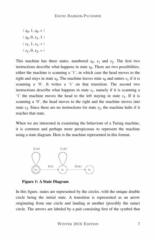
This machine has three states, numbered s0, s1 and s2. The first twoinstructions describe what happens in state s0. There are two possibilities,either the machine is scanning a ‘1’, in which case the head moves to theright and stays in state s0. The machine leaves state s0 and enters s1 if it isscanning a ‘0’. It writes a ‘1’ on that transition. The second twoinstructions describe what happens in state s1, namely if it is scanning a‘1’ the machine moves the head to the left staying in state s1. If it isscanning a ‘0’, the head moves to the right and the machine moves intostate s2. Since there are no instructions for state s2, the machine halts if itreaches that state.

When we are interested in examining the behaviour of a Turing machine,it is common and perhaps more perspicuous to represent the machineusing a state diagram. Here is the machine represented in this format.

In this figure, states are represented by the circles, with the unique doublecircle being the initial state. A transition is represented as an arroworiginating from one circle and landing at another (possibly the same)circle. The arrows are labeled by a pair consisting first of the symbol that

⟨ s0, 1, s0, » ⟩⟨ s0, 0, s1, 1 ⟩⟨ s1, 1, s1, « ⟩⟨ s1, 0, s2, » ⟩

Figure 1: A State Diagram



must be being scanned for the arrow to be followed, and second the actionthat is to be taken as the transition is made. The action will either be thesymbol to be written, or « or » indicating a move to the left or right.

In what follows we will describe Turing machines in the state machineformat.

2.1 Examples

In order to speak about a Turing machine that does something useful, wewill have to provide an interpretation of the symbols recorded on the tape.For example, if we want to design a machine which will perform somemathematical function, addition say, then we will need to describe how tointerpret the ones and zeros appearing on the tape as numbers.

In the examples that follow we will represent the number n as a block ofn+1 copies of the symbol ‘1’ on the tape. Thus we will represent thenumber 0 as a single ‘1’ and the number 3 as a block of four ‘1’s.

We will also have to make some assumptions about the configuration ofthe tape when the machine is started, and when it finishes, in order tointerpret the computation. We will assume that if the function to becomputed requires n arguments, then the Turing machine will start with itshead scanning the leftmost ‘1’ of a sequence of n blocks of ‘1’s. the blocksof ‘1’s representing the arguments must be separated by a singleoccurrence of the symbol ‘0’. For example, to compute the sum 3+4, aTuring machine will start in the following configuration, where the ellipsesindicate that the tape has only zeros on the cells that we can't see, and theupward arrow indicates the cell that is currently scanned.

Turing Machines


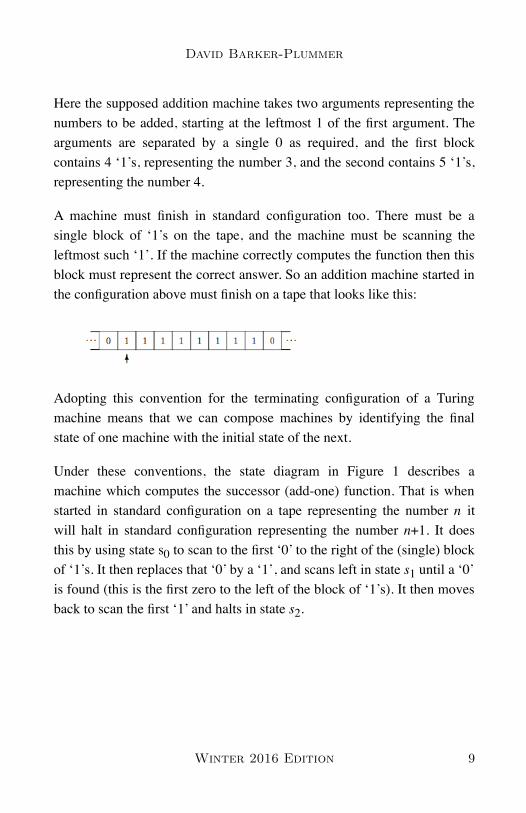
Here the supposed addition machine takes two arguments representing thenumbers to be added, starting at the leftmost 1 of the first argument. Thearguments are separated by a single 0 as required, and the first blockcontains 4 ‘1’s, representing the number 3, and the second contains 5 ‘1’s,representing the number 4.

A machine must finish in standard configuration too. There must be asingle block of ‘1’s on the tape, and the machine must be scanning theleftmost such ‘1’. If the machine correctly computes the function then thisblock must represent the correct answer. So an addition machine started inthe configuration above must finish on a tape that looks like this:

Adopting this convention for the terminating configuration of a Turingmachine means that we can compose machines by identifying the finalstate of one machine with the initial state of the next.

Under these conventions, the state diagram in Figure 1 describes amachine which computes the successor (add-one) function. That is whenstarted in standard configuration on a tape representing the number n itwill halt in standard configuration representing the number n+1. It doesthis by using state s0 to scan to the first ‘0’ to the right of the (single) blockof ‘1’s. It then replaces that ‘0’ by a ‘1’, and scans left in state s1 until a ‘0’is found (this is the first zero to the left of the block of ‘1’s). It then movesback to scan the first ‘1’ and halts in state s2.



Above, we see the initial state. Click on the image to see a movie of theexecution of the machine. (Click again to stop and reset.)

For another example, consider the machine in Figure 2 which computesthe addition function. That is, when started on a standard tape representingthe numbers n and m, the machine halts on a tape representing n+m.

Figure 2: A Machine for Computing n+m

Notice that this machine is like the add one machine in that states s0through s2 cause the machine to write a ‘1’ to the right of the first block of‘1’s, and returns the head to the leftmost ‘1’. In standard configuration foraddition, this joins the two blocks of ‘1’s into a single block, containing(n+1)+1+(m+1) copies of the symbol ‘1’, so that on entering state s2 thetape represents the number n+m+2. In order to correct this, we need to

Turing Machines


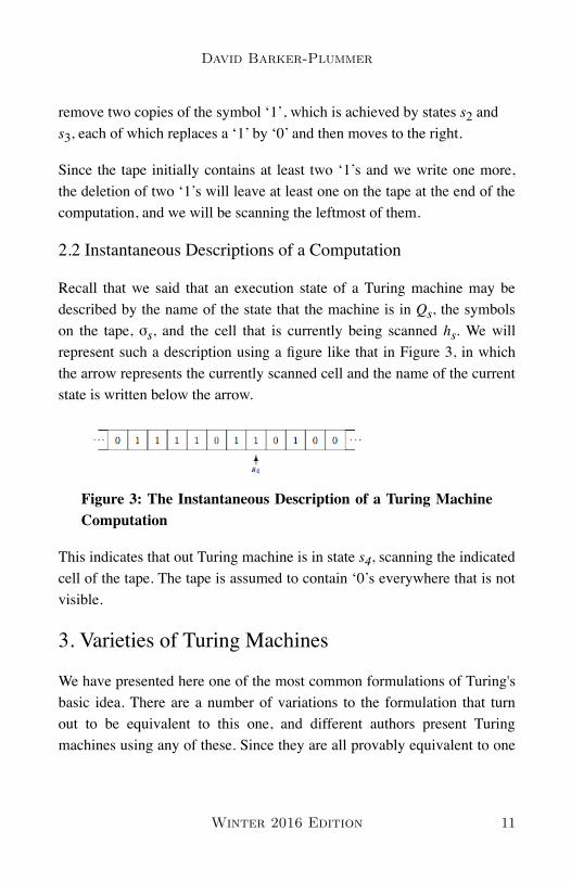
remove two copies of the symbol ‘1’, which is achieved by states s2 ands3, each of which replaces a ‘1’ by ‘0’ and then moves to the right.

Since the tape initially contains at least two ‘1’s and we write one more,the deletion of two ‘1’s will leave at least one on the tape at the end of thecomputation, and we will be scanning the leftmost of them.

2.2 Instantaneous Descriptions of a Computation

Recall that we said that an execution state of a Turing machine may bedescribed by the name of the state that the machine is in Qs, the symbolson the tape, σs, and the cell that is currently being scanned hs. We willrepresent such a description using a figure like that in Figure 3, in whichthe arrow represents the currently scanned cell and the name of the currentstate is written below the arrow.

This indicates that out Turing machine is in state s4, scanning the indicatedcell of the tape. The tape is assumed to contain ‘0’s everywhere that is notvisible.

3. Varieties of Turing Machines

We have presented here one of the most common formulations of Turing'sbasic idea. There are a number of variations to the formulation that turnout to be equivalent to this one, and different authors present Turingmachines using any of these. Since they are all provably equivalent to one

Figure 3: The Instantaneous Description of a Turing MachineComputation



another we can consider any of the formulations as being the definition ofTuring machine as we find convenient.

Formulation F1 and formulation F2 are equivalent if for every machinedescribed in formulation F1 there is machine a described in F2 which hasthe same input-output behavior, and vice versa, i.e., when started on thesame tape at the same cell, will terminate with the same tape on the samecell.

Two-way infinite tapes

In our original formulation we specified that the tape had an end, at the leftsay, and stretched infinitely far to the right. Relaxing this stipulation toallow the tape to stretch infinitely far to right and left results in a newformulation of Turing machines. You might expect that the additionalflexibility of having a two-way infinite tape would increase the number offunctions that could be computed, but it does not. If there is a machinewith a two-way infinite tape for computing some function, there there ismachine with a one-way infinite tape that will compute that same function.

Arbitrary numbers of read-write heads

Modifying the definition of a Turing machine so that the machine hasseveral read-write heads does not alter the notion of Turing-computability.

Multiple tapes

Instead of a single infinite tape, we could consider machines possessingmany such tapes. The formulation of such a machine would have to allowthe tuples to specify which tape is to be scanned, where the new symbol isto be written, and which tape head is to move. Again this formulation isequivalent to the original.

Two-dimensional tapes

Turing Machines


Instead of a one-dimensional infinite tape, we could consider a two-dimensional “tape”, which stretches infinitely far up and down as well asleft and right. We would add to the formulation that a machine transitioncan cause the read-write head to move up or down one cell in addition tobeing able to move left and right. Again this formulation is equivalent tothe original.

Arbitrary movement of the head

Modifying the definition of a Turing machine so that the read-write headmay move an arbitrary number of cells at any given transition does notalter the notion of Turing-computability.

Arbitrary finite alphabet

In our original formulation we allowed the use of only two symbols on thetape. In fact we do not increase the power of Turing machines by allowingthe use of any finite alphabet of symbols.

5-tuple formulation

A common way to describe Turing machines is to allow the machine toboth write and move its head in the same transition. This formulationrequires the 4-tuples of the original formulation to be replaced by 5-tuples

where Symbolnew is the symbol written, and Move is one of « and ».

Again, this additional freedom does not result in a new definition ofTuring-computable. For every one of the new machines there is one of theold machines with the same properties.

Non-deterministic Turing machines

⟨ State0, Symbol, Statenew, Symbolnew, Move ⟩



An apparently more radical reformulation of the notion of Turing machineallows the machine to explore alternatives computations in parallel. In theoriginal formulation we said that if the machine specified multipletransitions for a given state/symbol pair, and the machine was in such astate then it would halt. In this reformulation, all transitions are taken, andall the resulting computations are continued in parallel. One way tovisualize this is that the machine spawns an exact copy of itself and thetape for each alternative available transition, and each machine continuesthe computation. If any of the machines terminates successfully, then theentire computation terminates and inherits that machine's resulting tape.Notice the word successfully in the preceding sentence. In thisformulation, some states are designated as accepting states and when themachine terminates in one of these states, then the computation issuccessful, otherwise the computation is unsuccessful and any othermachines continue in their search for a successful outcome.

The addition of non-determinism to Turing machines does not alter thedefinition of Turing-computable.

Turing's original formulation of Turing Machines used the 5-tuplerepresentation of machines. Post introduced the 4-tuple representation, andthe use of a two-way infinite tape.

A more complex machine

In addition to performing numerical functions using unary representationfor numbers, we can perform tasks such as copying blocks of symbols,erasing blocks of symbols and so on. Here is an example of a Turingmachine which when started in standard configuration on a tape containinga single block of ‘1’s, halts on a tape containing two copies of that blockof ‘1’s, with the blocks separated by a single ‘0’. It uses an alphabetconsisting of the symbols ‘0’, ‘1’ and ‘A’.

Turing Machines


Figure 4: A Machine for Copying a Block of 1s

The action of this machine is to repeatedly change one of the original ‘1’sinto an A, and then write a new ‘1’ to the right of all remaining ‘1’ on thetape, after leaving a zero between the original block and the copy. Whenwe run out of the original ‘1’s, we turn the As back into ‘1’s.

The initial state, s0, is used to change a ‘1’ into an ‘A’, and move to theright and into state s1. In state s1 we skip the remainder of the block of ‘1’suntil we find a ‘0’ (the block separator) and in s2 we skip any ‘1’s to theright of that ‘0’ (this is the copy of the block of ‘1’s that we are making).When we reach the end of that block, we find a ‘0’, which we turn into a‘1’ and head back to the left, and into state s3. States s3 and s4 skip



leftward over the ‘1’s and separating ‘0’ on the tape until an ‘A’ is found.When this occurs, we go back into state s0, and move rightward.

At this point, we are either scanning the next ‘1’ of the original block, orthe original block has all been turned into ‘A's, and we are scanning theseparator ‘0’. In the former case, we make another trip through statess1–s4, but in the latter, we move into state s5, moving leftward. In thisstate we will repeatedly find ‘A's, which we replace with ‘1’s, and move tothe left. If we find a ‘0’, then all of the ‘A's have been turned back into‘1’s. We will be scanning the ‘0’ to the left of the original cell, and so wemove right, and into the final state s6.

This copying machine could be used in conjunction with the additionmachine of Figure 2 to construct a doubling machine, i.e., a machinewhich, when started on a tape representing the number n halts on a taperepresenting 2n. We could do this by first using the copying machine toproduce a tape with two copies of n on the tape, and then using theaddition machine to compute n+n (=2n). We would do this by identifyingthe copying machine's halt state (s6) with the adding machine's initial state(s0).

The construction just suggested relies on the fact that the copying machineterminates in standard position, which is required for the adding machineto correctly compute its result. By designing Turing machines which startand end in standard configuration, we can ensure that they may becomposed in this manner. In the example, the copying machine has aunique terminating state, but this is not necessary. We might build a Turingmachine which indicates the result of its computation by terminating onone of many states, and we can the combine that machine with more thatone machine, with the identity of the machine which follow dependent onthe switching machine. This would enable us to create a machine which

Turing Machines


adds one to the input if that input is even, and doubles it if odd, forexample (should we want to for some reason).

4. What Can Be Computed

Turing machines are very powerful. For a very large number ofcomputational problems, it is possible to build a Turing machine that willbe able to perform that computation. We have seen that it is possible todesign Turing machines for arithmetic on the natural numbers, forexample.

Computable Numbers

Turing's original paper concerned computable numbers. A number isTuring-computable if there exists a Turing machine which starting from ablank tape computes an arbitrarily precise approximation to that number.All of the algebraic numbers (roots of polynomials with algebraiccoefficients) and many transcendental mathematical constants, such as eand π are Turing-computable.

Computable Functions

As we have seen, Turing machines can do more than write down numbers.Among other things they can compute numeric functions, such as themachine for addition (presented in Figure 2) multiplication, propersubtraction, exponentiation, factorial and so on.

The characteristic function of a predicate is a function which has the valueTRUE or FALSE when given appropriate arguments. An example wouldbe the predicate ‘IsPrime’, whose characteristic function is TRUE whengiven a prime number, 2, 3, 5 etc and FALSE otherwise, for example whenthe argument is 4, 9, or 12. By adopting a convention for representingTRUE and FALSE, perhaps that TRUE is represented as a sequence of



two ‘1’s and FALSE as one ‘1’, we can design Turing-machines tocompute the characteristic functions of computable predicates. Forexample, we can design a Turing machine which when started on a taperepresenting a number terminates with TRUE on the tape if and only if theargument is a prime number. The results of such functions can becombined using the using the boolean functions: AND, NOT, OR, IF-THEN-ELSE, each of which is Turing-computable.

In fact the Turing-computable functions are just the recursive functions,described below.

Universal Turing Machines

The most striking positive result concerning the capabilities of Turingmachines is the existence of Universal Turing Machines (UTM). Whenstarted on a tape containing the encoding of another Turing machine, callit T, followed by the input to T, a UTM produces the same result as Twould when started on that input. Essentially a UTM can simulate thebehavior of any Turing machine (including itself).

One way to think of a UTM is as a programmable computer. When a UTMis given a program (a description of another machine), it makes itselfbehave as if it were that machine while processing the input.

Note again, our identification of input-output equivalence with “behavingidentically”. A machine T working on input t is likely to execute far fewertransitions that a UTM simulating T working on t, but for our purposes thisfact is irrelevant.

In order to design such a machine, it is first necessary to define a way ofrepresenting a Turing machine on the tape for the UTM to process. To dothis we will recall that Turing machines are formally represented as a

Turing Machines


collection of 4-tuples. We will first design an encoding for individualtuples, and then for sequences of tuples.

Encoding Turing Machines

Each 4-tuple in the machine specification will be encoded as a sequence offour blocks of ‘1’s, separated by a single ‘0’

1. The first block of ones will encode the current state number, using theunary number convention above (n+1 ones represents the number n).

2. The second block of ones will encode the current symbol, using one‘1’ to represent the symbol zero, and two to represent the symbol ‘1’(again because we can't use zero ones to represent ‘0’).

3. The third element of the tuple will represent the new state number inunary number notation.

4. The fourth element represents the action, and there are fourpossibilities: symbols will be encoded as above, with a block of three‘1’s representing a move to the left («) and a block of four ‘1’srepresenting a move to the right (»).

Using this convention the tuple ⟨0, ‘1’, 0, »⟩ would be represented as inFigure 5.

To encode a complete machine, we need to simply write down the tupleson the tape, in any order, but separated from one another by two blankcells so that we can tell where each tupe ends. The add-one machine ofFigure 1, would be represented by the somewhat intimidating string shownin Figure 6.

Figure 5: The Encoding of the Tuple ⟨⟨0, ‘1’, 0, »⟩⟩



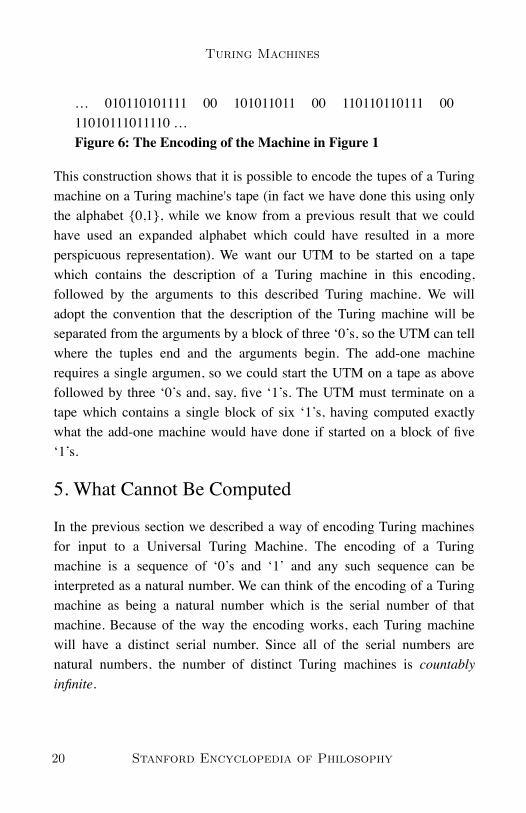
This construction shows that it is possible to encode the tupes of a Turingmachine on a Turing machine's tape (in fact we have done this using onlythe alphabet {0,1}, while we know from a previous result that we couldhave used an expanded alphabet which could have resulted in a moreperspicuous representation). We want our UTM to be started on a tapewhich contains the description of a Turing machine in this encoding,followed by the arguments to this described Turing machine. We willadopt the convention that the description of the Turing machine will beseparated from the arguments by a block of three ‘0’s, so the UTM can tellwhere the tuples end and the arguments begin. The add-one machinerequires a single argumen, so we could start the UTM on a tape as abovefollowed by three ‘0’s and, say, five ‘1’s. The UTM must terminate on atape which contains a single block of six ‘1’s, having computed exactlywhat the add-one machine would have done if started on a block of five‘1’s.

5. What Cannot Be Computed

In the previous section we described a way of encoding Turing machinesfor input to a Universal Turing Machine. The encoding of a Turingmachine is a sequence of ‘0’s and ‘1’ and any such sequence can beinterpreted as a natural number. We can think of the encoding of a Turingmachine as being a natural number which is the serial number of thatmachine. Because of the way the encoding works, each Turing machinewill have a distinct serial number. Since all of the serial numbers arenatural numbers, the number of distinct Turing machines is countablyinfinite.

… 010110101111 00 101011011 00 110110110111 0011010111011110 … Figure 6: The Encoding of the Machine in Figure 1

Turing Machines


On the other hand, the number of functions on the natural numbers isuncountable. There are (uncountably) more functions on the naturalnumbers than there are Turing machines, which shows that there areuncomputable functions, functions whose results cannot be computed byany Turing machine, because there are simply not enough Turingmachines to compute the functions.

This proof by counting is somewhat unsatisfactory, since it tells us thatthere are uncomputable functions, but provides us with no examples. Herewe give two examples of uncomputable functions.

5.1 The Busy Beaver

Imagine a Turing machine that is started on a completely blank tape, andeventually halts. If the machine leaves n ones on the tape when it halts, wewill say that the productivity of this machine is n. We will say that theproductivity of any machine that does not halt is 0. Productivity is afunction from Turing machine descriptions (natural numbers) to naturalnumbers. We will write p(T)=n to indicate that the productivity ofmachine T is n.

Among the Turing machines that have a particular number of states, thereis a maximum productivity that a Turing machine with that number ofstates can have. This too is a function from natural numbers (the numberof states) to natural numbers (the maximum productivity of a machinewith that number of states). We will write this function as BB(k)=n toindicate the maximum productivity of a k-state Turing machine is n. Theremay be multiple different k state machines with the maximum productivityn. We call any of these machines a Busy Beaver for k.

There is no Turing machine which will compute the function BB(k), i.e.,which when started in standard configuration on a tape with k ‘1’s will halt



in standard configuration on a tape with BB(k) ‘1’s. This example is due toTibor Radó (Radó 1962).

The proof that there is no such function proceeds by assuming that there issuch a machine, i.e. that there is a machine which starts in standardconfiguration with k ‘1’s on the tape, and halts in standard configurationwith BB(k) ‘1’s on the tape. We will call this machine B and assume that ithas k states.

There is an n-state machine which writes n ‘1’s on an initially blank tape(exercise for the reader). We can construct a new machine which connectsthe halting state of this machine to the start state of B and then connectingthe halting state of B to the start state of another copy of B. So the firstmachine writes n ‘1’ and then the first copy of B computes BB(n), but thenthe second copy of B takes over and computes BB(BB(n)). The totalnumber of states in our machine is n+2k. Our machine may be a BusyBeaver for n+2k, but it is certainly no more productive than such amachine. So (if the Busy Beaver machine exists)

It is easy to show that the productivity of Turing machines increases asstates are added, i.e.,

(another exercise). Consequently (if the Busy Beaver machine exists)

Since this is true for any n, it is true for n+11, yielding:

BB(n+2k) ≥ BB(BB(n)), for any n.

if i < j, then BB(i) < BB(j)

n+2k ≥ BB(n), for any n.

n+11+2k ≥ BB(n+11), for any n.

Turing Machines


But it is easy to show that BB(n+11) ≥ 2n (another exercise, but show thatthere is an eleven state machine for doubling the number of ‘1’ on the tape,and compose such a machine with the n-state machine for writing n ‘1’s).Combining this fact with the previous inequality we have:

from which by subtracting n from both sides we have 11+2k ≥ n, for any n,if the Busy Beaver exists, which is a contradiction.

Even though the productivity function is uncomputable, there isconsiderable interest in the search for Busy Beaver Turing machines (mostproductive machines with a given number of states). Some candidates canbe found by following links in the Other Internet resources section of thisarticle.

5.2 The Halting Problem

It would be very useful to be able to examine the description of a Turingmachine and determine whether it halts on a given input. This problem iscalled the Halting problem and is, regrettably, uncomputable. That is, noTuring machine exists which computes the function h(t,n) which is definedto be TRUE if machine t halts on input n and FALSE otherwise.

To see the uncomputability of the halting function, imagine that such amachine H exists, and consider a new machine built by composing thecopying machine of Figure 4 with H by joining the halt state of the copierto the start state of H. Such a machine, when started on a tape with n ‘1’sdetermines whether the machine whose code is n halts when given input n,i.e., it computes M(n) = h(n,n).

Now lets add another little machine to the halt state of H. This machinegoes into an infinite sequence of transitions if the tape contains TRUE

n+11+2k ≥ BB(n+11) ≥ 2n, for any n.



when it starts, and halts if the tape contains FALSE (its an exercise for thereader to construct this machine, assume that TRUE is represented by ‘11’,and FALSE by ‘1’).

This composed machine, call it M, halts if the machine with the input coden does not halt on an initial tape containing n (because if machine n doesnot halt on n, the halting machine will leave TRUE on the tape, and M willthen go into its infinite sequence), and vice versa.

To see that this is impossible, consider the code for M itself. What happenswhen M is started on a tape containing Ms code? Assume that M halts onM, then by the definition of the machine M it does not halt. But equally, ifit does not halt on M the definition of M says that it should halt.

This is a contradiction, and the Halting machine cannot exist. The fact thatthe halting problem is not Turing-computable was first proved by Turingin (Turing 1937b). Of course this result applies to real programs too. Thereis no computer program which can examine the code for a program anddetermine whether that program halts.

6. Alternative Formulations of Computability

6.1 Recursive Functions

Recursive function theory is the study of the functions that can be definedusing recursive techniques (see the entry on recursive functions). Briefly,the primitive recursive functions are those that can be formed from thebasic functions:

the zero function: z(x) = 0, for all xthe successor function: s(x) = x+1, for all xthe ith projection over j arguments: pi,j(x0,…xj) = xi, for all xi, i, j

Turing Machines


by using the operations of composition and primitive recursion:

Composition:

f(x1,…,xn) = g(h1(x1,…,xn),…, hm(x1,…,xn)), for all g,h1,…,hm

Primitive Recursion:f(x,0) = g(x), for any g

f(x,s(y)) = h(x,y,f(x,y)), for any h

The recursive functions are formed by the addition of the minimizationoperator, which takes a function f and returns h defined as follows:

Minimization:h(x1,…,xn) = y, if f(x1, …,xn,y)=0 and ∀t<y(f(x1, …,xn,t) is defined

and positive)= undefined otherwise.

It is known that the Turing computable functions are exactly the recursivefunctions.

6.2 Abacus Machines

Abacus machines abstract from the more familiar architecture of themodern digital computer (the von Neumann architecture). In its simplestform a computer with such an architecture has a number of addressableregisters each of which can hold a single datum, and a processor whichcan read and write to these registers.

The machine can perform two basic operations, namely: add one to thecontent of a named register (which we will symbolize as n+, where n isthe name of the register) and (attempt to) subtract one from a namedregister, with two possible outcomes: a success branch if the register was



initially non-zero, and a failure branch if the register was initially zero (wewill symbolize the operation as n-).

These are called abacus computers by Lambek (Lambek 1961), and areknown to be equivalent to Turing machines.

The modern digital computer is subject to finiteness constraints that wehave abstracted away in the definition of abacus machines, just as we didin the case of Turing machines. Physical computers are limited in thenumber of memory locations that they have, and in the storage capacity ofeach of those locations, while abacus machines are not subject to thoseconstraints. Thus some abacus-computable functions will not becomputable by any physical machine. (We won't consider whether Turingmachines and modern digital computers remain equivalent when both aregiven external inputs, since that would require us to change the definitionof a Turing machine.)

7. Restricted Turing Machines

One way to modify the definition of Turing machines is by removing theirability to write to the tape. The resulting machines are called finite statemachines. They are provably less powerful than Turing machines, sincethey cannot use the tape to remember the state of the computation. Forexample, finite state machines cannot determine whether an input stringconsists of some As followed by the same number of Bs. The reason isthat the machine cannot remember how many As it has seen so far, exceptby being in a state that represents this fact, and determining whether thenumber of As and Bs match in all cases would require the machine to haveinfinitely many states (one to remember that it has seen one A, one toremember that it has seen 2, and so on).

Turing Machines


Bibliography

Barwise, J. and Etchemendy, J., 1993, Turing's World, Stanford: CSLIPublications.

Boolos, G.S. and Jeffrey, R.C., 1974, Computability and Logic,Cambridge: Cambridge University Press.

Davis, M., 1958, Computability and Unsolvability, New York: McGraw-Hill; reprinted Dover, 1982.

Herken, R., (ed.), 1988, The Universal Turing Machine: A Half-CenturySurvey, New York: Oxford University Press.

Hodges, A., 1983, Alan Turing, The Enigma, New York: Simon andSchuster.

Kleene, S.C., 1936, “General Recursive Functions of Natural Numbers,”Mathematische Annalen, 112: 727–742.

Lambek, J., 1961, “How to Program an Infinite Abacus,” CanadianMathematical Bulletin, 4: 279–293.

Lewis, H.R. and Papadimitriou, C.H., 1981, Elements of the Theory ofComputation, Englewood Cliffs, NJ: Prentice-Hall.

Lin, S. and Radó, T., 1965, “Computer Studies of Turing MachineProblems,” Journal of the Association for Computing Machinery, 12:196–212.

Petzold, G., 2008, “The Annotated Turing: A Guided Tour Through AlanTuring's Historic Paper on Computability and Turing Machines,”,Indianapolis, Indiana: Wiley.

Post, E., 1947, “Recursive Unsolvability of a Problem of Thue,” TheJournal of Symbolic Logic, 12: 1–11.

Radó, T., 1962, “On Non-computable functions,” Bell System TechnicalJournal, 41 (May): 877–884.

Turing, A.M., 1937a, “On Computable Numbers, With an Application tothe Entscheidungsproblem,” Proceedings of the LondonMathematical Society, s2-42 (1): 230–265; correction ibid., (1938)



s2-43 (1): 544–546. [Note: This paper was received May 28, 1936and read to the Society on November 12, 1936, but wasn't actuallypublished until 1937.]

Turing, A.M., 1937b, “Computability and λ-Definability,” The Journal ofSymbolic Logic, 2: 153–163.

Academic Tools

Other Internet Resources

“Turing Machines”, Stanford Encyclopedia of Philosophy (Summer2003 Edition), Edward N. Zalta (ed.), URL =<https://plato.stanford.edu/archives/sum2003/entries/turing-machine/>. [This was the original version of the present entry, writtenby the Editors of the Stanford Encyclopedia of Philosophy.]The Alan Turing Home PageBletchley Park, in the U.K., where, during the Second World War,Alan Turing was involved in code breaking activites at Station X.

Busy Beaver

Michael Somos' page of Busy Beaver references.

The Halting Problem

How to cite this entry.Preview the PDF version of this entry at the Friends of the SEPSociety.Look up this entry topic at the Indiana Philosophy OntologyProject (InPhO).Enhanced bibliography for this entry at PhilPapers, with linksto its database.

Turing Machines


Halting problem solvable (funny)

Online Turing Machine Simulators

Turing machines are more powerful than any device that can actually bebuilt, but they can be simulated both in software and hardware.

Software Simulators

There are many Turing machine simulators available. Here are threesoftware simulators that use different technologies to implementsimulators using your browser.

Andrew Hodges' Turing Machine Simulator (for limited number ofmachines)Suzanne Britton's Turing Machine Simulator (A Java Applet)

Here is an application that you can run on the desktop (no endorsement ofthese programs is implied).

Visual Turing: freeware simulator for Windows 95/98/NT/2000

Hardware Simulators

Turing Machine in the Classic Style, Mike Davey's physical Turingmachine simulator.Lego of Doom, Turing machine simulator using Lego™.A purely mechanical Turing Machine, Computer ScienceDepartment, École Normal Supérieure de Lyon. (This one has noembedded microprocessor.)

Related Entries



Church, Alonzo | Church-Turing Thesis | computability and complexity |function: recursive | Turing, Alan

Copyright © 2016 by the author David Barker-Plummer

Turing Machines


Documents

Stanford Encyclopedia of Philosophy Edward N. … Stanford Encyclopedia of Philosophy. 1. A DeÞnition of Turing Machines A Turing machine is a kind of state machine . At any time