Embed Size (px)
Citation preview

1 | P a g e
Standard Time Signals - GATE Study
Material in PDF
In the previous article, we discussed Time Signals & Signal Transformation. In these
free GATE 2018 Notes, we will discuss some Important Standard Time Signals.
These continuous signals are used in problem solving and analysis. These study
notes are important for GATE EC and GATE EE as well as other exams like BARC,
BSNL, DRDO, ISRO, IES etc. These notes may also be downloaded in PDF so that
your exam preparation is made easy and you ace your exam.
You are strongly advised to go through previous articles before starting off with this
module.
Recommended Reading –
Laplace Transforms
Limits, Continuity & Differentiability
Mean Value Theorems
Differentiation
Partial Differentiation
Maxima and Minima
Methods of Integration & Standard Integrals
Vector Calculus
Vector Integration
Time Signals & Signal Transformation
2 | P a g e
Standard Continuous Time Signals Some of the standard continuous time signals covered here include:
1. DC Signal
2. Unit Step Signal
3. Unit Impulse / Delta Signal
4. Ramp Signal
5. Signum Signal
6. Rectangular Pulse or Gate Function
7. Triangular Function
8. Sinusoidal Function
9. Sampling Function
10. Sinc Function
11. Exponential Function
DC Signal
It is given as for both continuous and discrete signals
x(t) = A ; –∞ < t < ∞
x[n] = A ; –∞ < n < ∞
Unit Step Signal
Continuous time unit step signal is defined as

3 | P a g e
u(t) = {1 ; t ≥ 00 ; t > 0
Similar concept is followed in discrete time unit step signal.
Unit Impulse / Delta Signal
It is defined as
δ(t) = {1; t = 00; t ≠ 0
and ∫ δ(t) = 1∞
−∞
Similarly, you can derive for discrete time delta signal. Some properties of
continuous time delta signal are given as follows
(𝐢) δ(at) =1
|a|δ(t)
(𝐢𝐢) x(t)δ(t − t0) = x(t0)δ(t − t0)
(𝐢𝐢𝐢) ∫ x(t)δ(t − t0)dt∞
−∞= x(t0)

4 | P a g e
(𝐢𝐯) δ(t) =d
dt(u(t))
(𝐯) u(t) = ∫ δ(t)dtt
−∞
(𝐯𝐢) x(t) ∗ δ(t) = u(t) [Replication Property of Delta Signal]
The properties for discrete time impulse signal are a bit different for some. These are
(i) δ[an] = δ[n]
(ii) x[n] δ[n-k] = x[k] δ[n-k]
(iii) δ[n] = u[n] - u[n-1]
(𝐢𝐯) u[n] = ∑ δ[k] = ∑ δ[n − k]nk=0
nk=−∞
The derivative and integral of singular or non-analytic functions are determined
using indirect method. Since impulse is a singular function. Therefore, to
determine its derivative, first we approximate it by a pulse of width ‘a’ and height
‘1/a’ and as ‘a’ tends to zero we get the continuous delta function. So we can say
that the unit impulse function is sometimes approximated to a delta function. A delta
function can be shown as follows:
Area of a delta function is 1.
δ(t) = lima→0
x(t)
x(t) =1
a{u (t +
a
2) − u (t −
a
2)}
Doublet:

5 | P a g e
The derivative of the impulse function is known as the Doublet.
δ(t) = lim a→0
x(t)
dδ(t)
dt= δ′(t) = lim
a→0
dx(t)
dt
= lim a→0
1
𝑎
d
dt[u (t +
a
2) − u (t −
a
2)] = lim
a→0(
d
dtu (t +
a
2) −
d
dtu (t −
a
2)) ×
1
a
⇒ δ′(t) = lima→0
1
aδ (t +
𝑎
2) − lim
a→0
1
aδ (t −
a
2)
Combination of two impulses is known as doublet.
δ'(t)→ Doublet, δ''(t) → Quadraplet, δ'''(t) → Octaplet
The properties of doublet are as below –
(𝐢) δ′(t) = {0; t ≠ 0 undefined; t = 0
} and ∫ δ′(t)dt = 0∞
−∞
(𝐢𝐢) δ′(at) = 1
a|a|δ′(t)
(𝐢𝐢𝐢) δ′(a(t − t0)) = 1
a|a|δ′(t − t0)
(𝐢𝐯) δ′(−t) = −δ′(t)
(𝐯) δ′(−(t − t0)) = −δ′(t − t0)
(𝐯𝐢) ∫ x(t)δ′(t)dt = −x′(0)∞
−∞

6 | P a g e
Ramp Signal
A continuous time ramp signal is defined as
r(t) = {t; t ≥ 00; t < 0
Or r(t) = t u(t)
Its value increases linearly with time.
1. Subtraction of the ramp signal decreases the slope.
2. Addition of the ramp signal increases the slope.
Also, u(t) =dr(t)
dt or r(t) = ∫ u(t)dt
t
−∞
Similarly, try to derive for discrete time ramp signal. We can see some transformed
signals from r(t).

7 | P a g e
Signum Signal
Continuous time signum signal is defined as
sgn(t) = {1; t > 0−1; t < 00; t = 0
It can also be written as
sgn(t) = u(t) - u(-t)
The phenomenon is similar in discrete time signum signal.
Rectangular Pulse or Gate Function
Continuous time rectangular pulse function is denoted by
A rect (t−t0
τ) /A gate (
t−t0
τ)
Here A = Amplitude, t0 = Centre, τ = Width
If centre is at origin, then it is defined as
A rect (t
τ) = {
A; |t| ≤τ
2
0; otherwise

8 | P a g e
Kindly note the difference between the continuous time and discrete time signals in
this
case.
Discrete time rectangular gate function is defined as
A rect (n−n0
N) OR A gate (
n−n0
N)
Where A = Amplitude, n0 = Centre of the pulse
N = Number of samples to the right ride from the centre or the number of samples to
the left side from the centre.
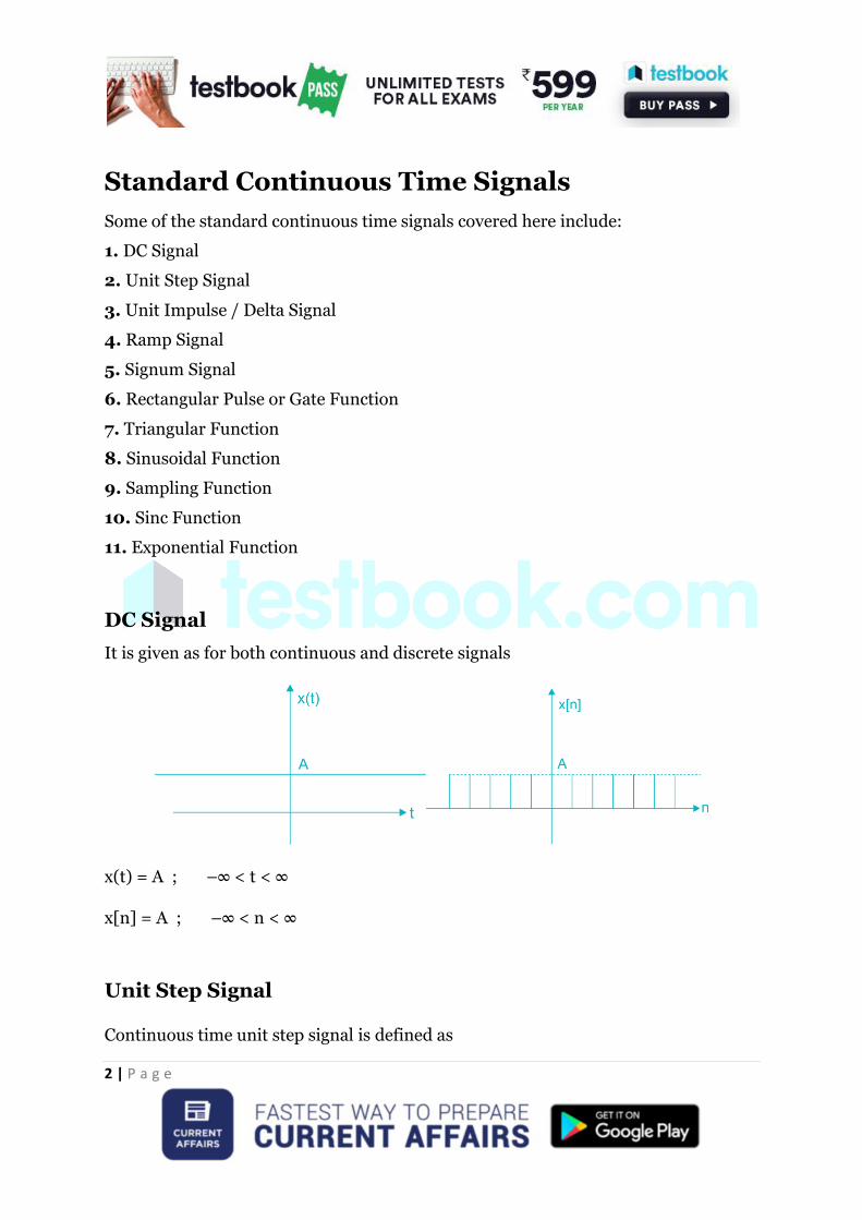
Triangular Function
Continuous time triangular function is denoted by A tri (t−t0
τ ) or A ∆ (
t−t0
τ)
Where A = Height of the signal, t0 = centre, τ = Half width
9 | P a g e
Discrete triangular time signal is similar to the continuous triangular time signal.
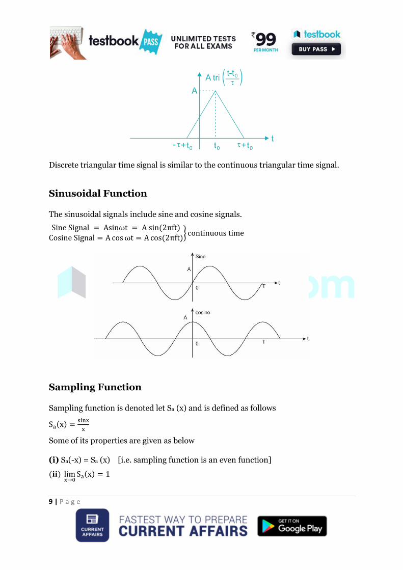
Sinusoidal Function
The sinusoidal signals include sine and cosine signals.
Sine Signal = Asinωt = A sin(2πft)Cosine Signal = A cos ωt = A cos(2πft)
} continuous time
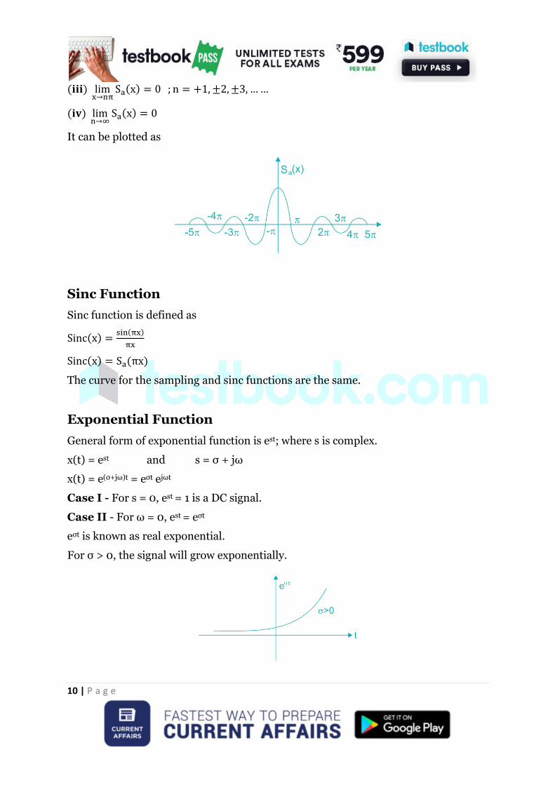
Sampling Function
Sampling function is denoted let Sa (x) and is defined as follows
Sa(x) =sinx
x
Some of its properties are given as below
(i) Sa(-x) = Sa (x) [i.e. sampling function is an even function]
(𝐢𝐢) limx→0
Sa(x) = 1
10 | P a g e
(𝐢𝐢𝐢) limx→nπ
Sa(x) = 0 ; n = +1, ±2, ±3, … …
(𝐢𝐯) limn→∞
Sa(x) = 0
It can be plotted as
Sinc Function Sinc function is defined as
Sinc(x) =sin(πx)
πx
Sinc(x) = Sa(πx)
The curve for the sampling and sinc functions are the same.
Exponential Function
General form of exponential function is est; where s is complex.
x(t) = est and s = σ + jω
x(t) = e(σ+jω)t = eσt ejωt
Case I - For s = 0, est = 1 is a DC signal.
Case II - For ω = 0, est = eσt
eσt is known as real exponential.
For σ > 0, the signal will grow exponentially.

11 | P a g e
For σ < 0, the signal will be decaying exponential.
Case III - For σ = 0 & ω ≠ 0, ejωt will be a periodic complex exponential with period
T0 =2π
ω
𝐂𝐚𝐬𝐞 𝐈𝐕 − For σ ≠ 0 & ω ≠ 0x(t) = eσtejωt
For σ > 0
Re(x(t)) = eσt cosωt is a growing sinusoidal
For σ < 0
Re(x(t)) = eσt cosωt is a decaying sinusoidal

12 | P a g e
Similar phenomenon is followed in discrete time equivalent of exponential signals.
Let us try out some examples now -
Example 1:
Simplify δ(t2 – 3t + 2)
Solution:
x(t) = δ(t2 – 3t + 2)
f(t) = t2 – 3t + 2 = (t – 2)(t – 1)
f(t) has two roots at t = 1,2
f' (t) = 2t – 3
f' (1) = 2×1 – 3 = –1
f' (2) = 2×2 – 3 = 1
So, δ(t2 − 3t + 2) = 1
|f′(t1)|δ(t − t1) +
1
|f′(t2)|δ(t − t2)
Here,
t1 = 1 and f' (t1) = –1
t2 = 2 and f' (t2) = 1
⇒ δ(t2 − 3t + 2) = 1
|−1|δ(t − 1) +
1
|1|δ(t − 2)
⇒ δ(t2 − 3t + 2) = δ(t − 1) + δ(t − 2)

13 | P a g e
Example 2:
Simplify the following
(i) δ’(–4t)
(ii) δ’(–3t–2)
(iii) δ’(t) e–3t
(iv) ∫ e−4t∞
−∞δ′(t)dt
Solution:
(i) δ′(−4t) =1
−4|−4|δ′(t) = −
1
16δ′(t)
(ii) δ′(−3t − 2) = δ′ (−3(t + 23⁄ )) =
1
−3|−3|δ′(t + 2
3⁄ ) = −1
9δ′(t + 2
3⁄ )
(iii) δ’(t). e−3t
Since, x(t). δ′(t) = x(0)δ′(t) − x′(0)δ(t)
Therefore, e−3tδ′(t) = 1. δ′(t) − (−3 × 1) × δ(t) = δ’(t) + 3δ(t)
(iv) ∫ e−4t∞
−∞δ′(t)dt = −
d
dte−4t|
t=0= 4
Example 3:
Sketch the derivative of x(t)

14 | P a g e
Solution:
x(t) = 3u(t + 2) − 5u(t − 3) + 2u(t − 4)
x′(t) = 3δ(t + 2) − 5δ(t − 3) + 2δ(t − 4)
Thus, we listed some of the important standard signals important for competitive
exam point of view. After this, we will discuss the classification of signals based on
their properties.
Example 4:
Sketch the following
(i) r(-t) (ii) - r(-t) (iii) r(t-2) (iv) r(-t+1)
(v) r(2t) (vi) 3r(t) (vii) r(2t-3) (viii) r(-2t-3)
(ix) d
dtr(t)
Solution:

15 | P a g e
𝐢) 𝐢𝐢)
𝐢𝐢𝐢) 𝐢𝐯)
𝐯) 𝐯𝐢)
𝐯𝐢𝐢) 𝐯𝐢𝐢𝐢)

16 | P a g e
𝐢𝐱)
Example 5:
Sketch the following signals
(i) r(t)+u(t)
(ii) r(t) - u(t)
(iii) r(t) + 2u(t-2)
(iv) r(t)- 2u(t-3)
Solution:
(i) r(t) +u(t)
r(t)+u(t) = tu(t) + u(t) = (t+1) u(t)
(ii) r(t) – u(t)
r(t)+ u(t) = (t-1)u(t)

17 | P a g e
(iii) r(t)+2u(t-2)
(iv) r(t) – 2r(t-3)
Example 6:
Write the expression of the following signals in the form of step and ramp signals?
(i)
(ii)
(iii)

18 | P a g e
Solution:
(i)
=2
3r(t) −
2
3r(t − 3)
(ii)
=3
2r(t) −
3
2r(t − 2) − 3u(t − 5)
(iii)
=A
Tr(t) −
A
Tr(t − T) − Au(t − T)

19 | P a g e
Example 7:
Sketch the following signals
(i) 5rect (t−1
2)
(ii) 2gate (2t + 5)
Solution:
(i) 5rect (t−1
2)
Here, τ = 2 and t0 = 1
First plot 5 rect (t
2)
Now shift this to right by 1 unit
(ii) 2gate(2t+5) = 2gate(2(t+5/2))
here, τ = 12⁄ and t0 = −5/2
First plot 2gate (2t)
20 | P a g e
Now shift this to left by 5⁄2 unit
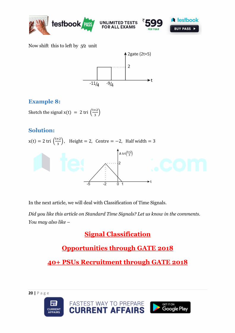
Example 8:
Sketch the signal x(t) = 2 tri (t+2
3)
Solution:
x(t) = 2 tri (t+2
3) , Height = 2, Centre = −2, Half width = 3
In the next article, we will deal with Classification of Time Signals.
Did you like this article on Standard Time Signals? Let us know in the comments.
You may also like –
Signal Classification
Opportunities through GATE 2018
40+ PSUs Recruitment through GATE 2018