Discrete-Time Signals and Systems - Department of EEhcso/ee4219_3.pdf · Discrete-Time Signals and Systems. ... Understanding deterministic and random discrete-time signals and ability

Discrete-Time Signals and Systems

Chapter Intended Learning Outcomes: (i) Understanding deterministic and random discrete-time signals and ability to generate them (ii) Ability to recognize the discrete-time system properties, namely, memorylessness, stability, causality, linearity and time-invariance (iii) Understanding discrete-time convolution and ability to perform its computation (iv) Understanding the relationship between difference equations and discrete-time signals and systems H. C. So Page 1 Semester B, 2013-2014

Discrete-Time Signal

Discrete-time signal can be generated using a computing software such as MATLAB It can also be obtained from sampling continuous-time

signals in real world

t

Fig.3.1:Discrete-time signal obtained from analog signal H. C. So Page 2 Semester B, 2013-2014

The discrete-time signal is equal to only at the sampling interval of ,

(3.1)

where is called the sampling period

is a sequence of numbers, , with being the time index

Basic Sequences

Unit Sample (or Impulse) (3.2)

H. C. So Page 3 Semester B, 2013-2014

It is similar to the continuous-time unit impulse which is defined in (2.10)-(2.12)

is simpler than because it is well defined for all while is not defined at

Unit Step (3.3)

It is similar to to the continuous-time of (2.13)

is well defined for all but is not defined . H. C. So Page 4 Semester B, 2013-2014

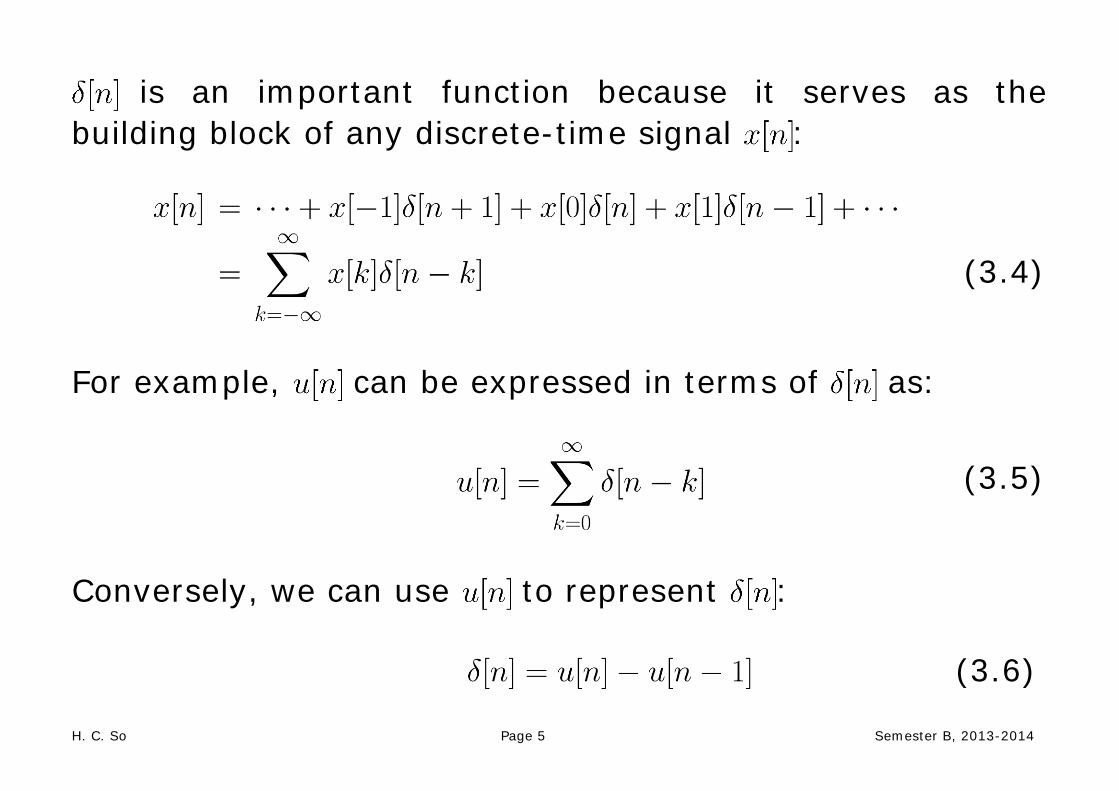
is an important function because it serves as the building block of any discrete-time signal :

(3.4)

For example, can be expressed in terms of as:

(3.5)

Conversely, we can use to represent : (3.6)


Introduction to MATLAB

MATLAB stands for ”Matrix Laboratory”

Interactive matrix-based software for numerical and symbolic computation in scientific and engineering applications

Its user interface is relatively simple to use, e.g., we can use the help command to understand the usage and syntax of each MATLAB function

Together with the availability of numerous toolboxes, there are many useful and powerful commands for various disciplines

MathWorks offers MATLAB to C conversion utility

Similar packages include Maple and Mathematica


Discrete-Time Signal Generation using MATLAB

A deterministic discrete-time signal satisfies a generating model with known functional form:

(3.7)

where is a function of parameter vector and time index . That is, given and , can be produced

e.g., the time-shifted unit sample and unit step function , where the parameter is

e.g., for an exponential function , we have where is the decay factor and is the time shift

e.g., for a sinusoid , we have


Example 3.1 Use MATLAB to generate a discrete-time sinusoid of the form:

with , , and , which has a duration of 21 samples

We can generate by using the following MATLAB code:

N=21; %number of samples is 21 A=1; %tone amplitude is 1 w=0.3; %frequency is 0.3 p=1; %phase is 1 for n=1:N x(n)=A*cos(w*(n-1)+p); %time index should be >0 end Note that x is a vector and its index should be at least 1. H. C. So Page 8 Semester B, 2013-2014

Alternatively, we can also use:

N=21; %number of samples is 21 A=1; %tone amplitude is 1 w=0.3; %frequency is 0.3 p=1; %phase is 1 n=0:N-1; %define time index vector x=A.*cos(w.*n+p); %first time index is also 1

Both give x =

Columns 1 through 7

0.5403 0.2675 -0.0292 -0.3233 -0.5885 -0.8011 -0.9422

Columns 8 through 14

-0.9991 -0.9668 -0.8481 -0.6536 -0.4008 -0.1122 0.1865

Columns 15 through 21

0.4685 0.7087 0.8855 0.9833 0.9932 0.9144 0.7539

Which approach is better? Why?


To plot , we can either use the commands stem(x) and plot(x)

If the time index is not specified, the default start time is

Nevertheless, it is easy to include the time index vector in the plotting command

e.g., Using stem to plot with the correct time index:

n=0:N-1; %n is vector of time index stem(n,x) %plot x versus n

Similarly, plot(n,x) can be employed to show The MATLAB programs for this example are provided as ex3_1.m and ex3_1_2.m H. C. So Page 10 Semester B, 2013-2014

0 5 10 15 20-1

-0.8

-0.6

-0.4

-0.2

0

0.2

0.4

0.6

0.8

1

n

x[n]

Fig.3.2: Plot of discrete-time sinusoid using stem


0 5 10 15 20-1

-0.8

-0.6

-0.4

-0.2

0

0.2

0.4

0.6

0.8

1

n

x[n]

Fig.3.3: Plot of discrete-time sinusoid using plot


Apart from deterministic signal, random signal is another importance signal class. It cannot be described by mathematical expressions like deterministic signals but is characterized by its probability density function (PDF). MATLAB has commands to produce two common random signals, namely, uniform and Gaussian (normal) variables.

A uniform integer sequence whose values are uniformly distributed between 0 and , can be generated using:

(3.8)

where and are very large positive integers, is the reminder of dividing by

Each admissible value of has the same probability of occurrence of approximately H. C. So Page 13 Semester B, 2013-2014

We also need an initial integer or seed, say, , for starting the generation of

(3.8) can be easily modified by properly scaling and shifting

e.g., a random number which is uniformly between –0.5 and 0.5, denoted by , is obtained from :

(3.9)

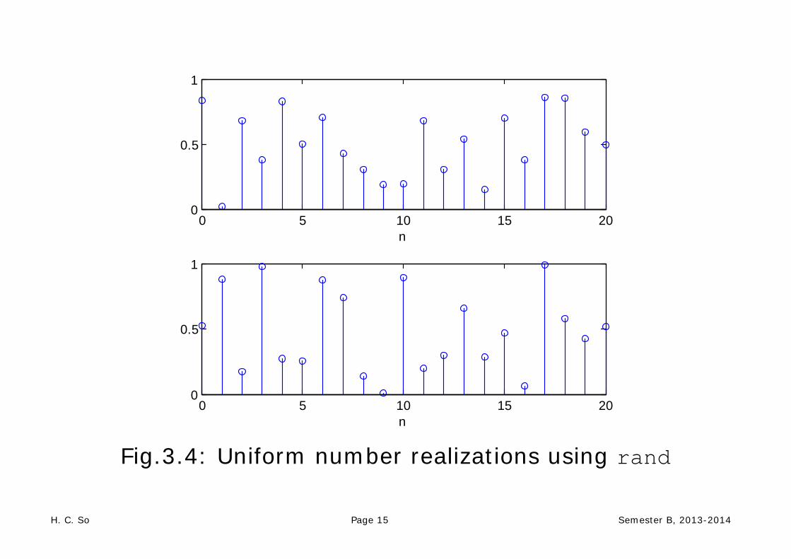
The MATLAB command rand is used to generate random numbers which are uniformly between 0 and 1

e.g., each realization of stem(0:20,rand(1,21)) gives a distinct and random sequence, with values are bounded between 0 and 1 H. C. So Page 14 Semester B, 2013-2014

0 5 10 15 200

0.5

1

n

0 5 10 15 200

0.5

1

n

Fig.3.4: Uniform number realizations using rand H. C. So Page 15 Semester B, 2013-2014

Example 3.2 Use MATLAB to generate a sequence of 10000 random numbers uniformly distributed between –0.5 and 0.5 based on the command rand. Verify its characteristics. According to (3.9), we use u=rand(1,10000)-0.5 to generate the sequence To verify the uniform distribution, we use hist(u,10), which bins the elements of u into 10 equally-spaced containers We see all numbers are bounded between –0.5 and 0.5, and each bar which corresponds to a range of 0.1, contains approximately 1000 elements. H. C. So Page 16 Semester B, 2013-2014

-0.5 0 0.50

200

400

600

800

1000

1200

Fig.3.5: Histogram for uniform sequence


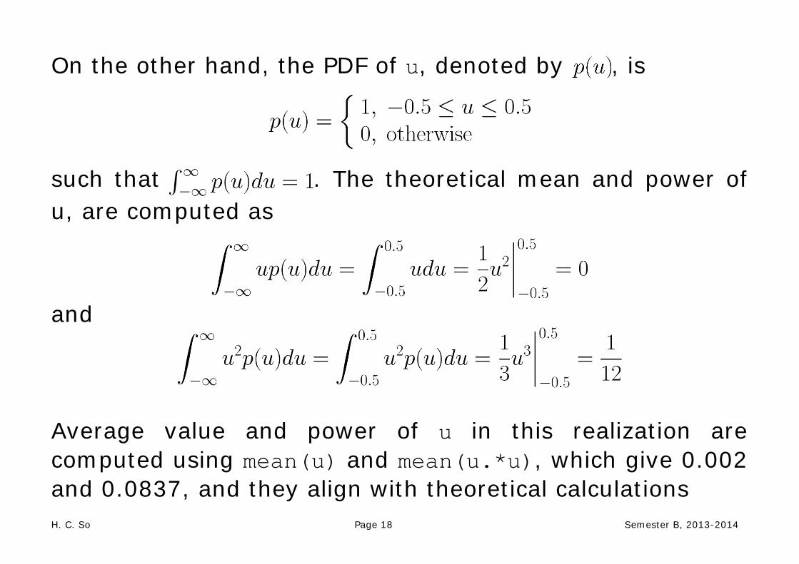
On the other hand, the PDF of u, denoted by , is

such that . The theoretical mean and power of u, are computed as

and

Average value and power of u in this realization are computed using mean(u) and mean(u.*u), which give 0.002 and 0.0837, and they align with theoretical calculations H. C. So Page 18 Semester B, 2013-2014

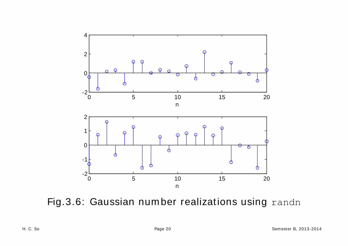
Gaussian numbers can be generated from the uniform variables

Given a pair of independent random numbers uniformly distributed between 0 and 1, , a pair of independent Gaussian numbers , which have zero mean and unity power (or variance), can be generated from:

(3.10) and

(3.11)

The MATLAB command is randn. Equations (3.10) and (3.11) are known as the Box-Mueller transformation

e.g., each realization of stem(0:20,randn(1,21)) gives a distinct and random sequence, whose values are fluctuating around zero H. C. So Page 19 Semester B, 2013-2014

0 5 10 15 20-2

0

2

4

n

0 5 10 15 20-2

-1

0

1

2

n

Fig.3.6: Gaussian number realizations using randn H. C. So Page 20 Semester B, 2013-2014

Example 3.3 Use the MATLAB command randn to generate a zero-mean Gaussian sequence of length 10000 and unity power. Verify its characteristics. We use w=randn(1,10000) to generate the sequence and hist(w,50) to show its distribution The distribution aligns with Gaussian variables which is indicated by the bell shape The empirical mean and power of w computed using mean(w) and mean(w.*w) are and 1.0028 The theoretical standard deviation is 1 and we see that most of the values are within –3 and 3 H. C. So Page 21 Semester B, 2013-2014

-4 -3 -2 -1 0 1 2 3 40

100

200

300

400

500

600

700

Fig.3.7: Histogram for Gaussian sequence


Discrete-Time Systems

A discrete-time system is an operator which maps an input sequence into an output sequence :

(3.12)

Memoryless: at time depends only on at time

Are they memoryless systems?

y[n]=(x[n])2

y[n]=x[n]+ x[n-2]

Linear: obey principle of superposition, i.e., if

and then

(3.13) H. C. So Page 23 Semester B, 2013-2014

Example 3.4 Determine whether the following system with input and output , is linear or not:

A standard approach to determine the linearity of a system is given as follows. Let

with

If , then the system is linear. Otherwise, the system is nonlinear. H. C. So Page 24 Semester B, 2013-2014

Assigning , we have:

Note that the outputs for and are and As a result, the system is linear


Example 3.5 Determine whether the following system with input and output , is linear or not:

The system outputs for and are and . Assigning

, its system output is then:

As a result, the system is nonlinear H. C. So Page 26 Semester B, 2013-2014

Time-Invariant: a time-shift of input causes a corresponding shift in output, i.e., if

then

(3.14) Example 3.6 Determine whether the following system with input and output , is time-invariant or not:

A standard approach to determine the time-invariance of a system is given as follows. H. C. So Page 27 Semester B, 2013-2014

Let

with

If , then the system is time-invariant. Otherwise, the system is time-variant.

From the given input-output relationship, is:

Let , its system output is:

As a result, the system is time-invariant. H. C. So Page 28 Semester B, 2013-2014

Example 3.7 Determine whether the following system with input and output , is time-invariant or not:

From the given input-output relationship, is of the form:

Let , its system output is:

As a result, the system is time-variant.


Causal: output at time depends on input up to time

For linear time-invariant (LTI) systems, there is an alternative definition. A LTI system is causal if its impulse response satisfies:

(3.15)

Are they causal systems?

y[n]=x[n]+x[n+1]

y[n]=x[n]+x[n-2]

Stable: a bounded input ( ) produces a bounded output ( )


For LTI system, stability also corresponds to

(3.16)

Are they stable systems?

y[n]=x[n]+x[n+1]

y[n]=1/x[n]

Convolution

The input-output relationship for a LTI system is characterized by convolution:

(3.17)

which is similar to (2.23)


(3.17) is simpler as it only needs additions and multiplications

specifies the functionality of the system

Commutative

(3.18)

and

(3.19)


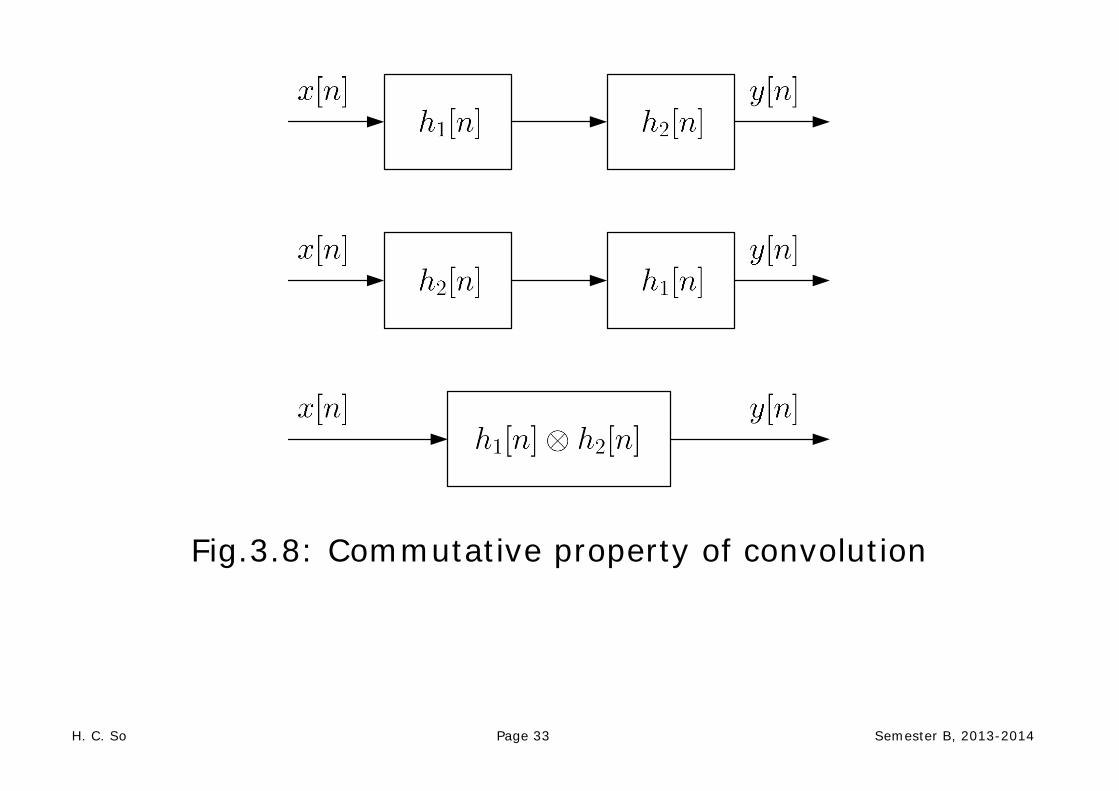
Fig.3.8: Commutative property of convolution


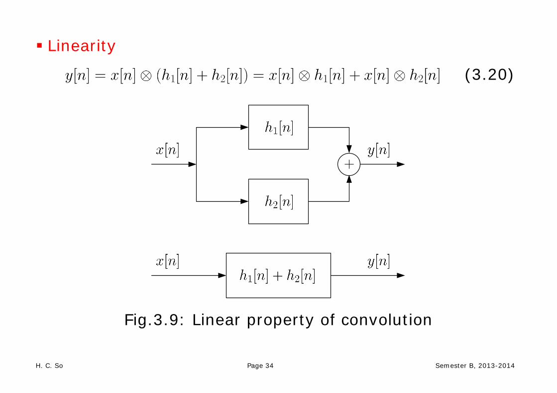
Linearity

(3.20)

Fig.3.9: Linear property of convolution H. C. So Page 34 Semester B, 2013-2014

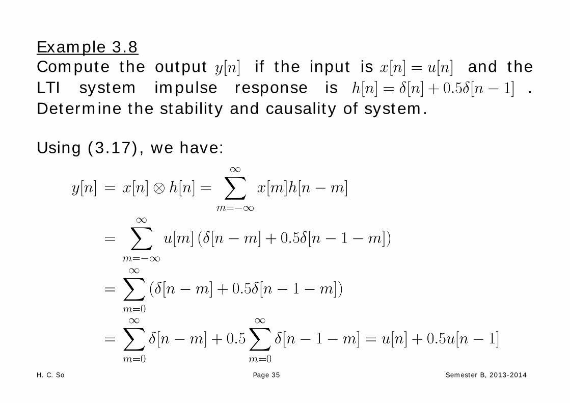
Example 3.8 Compute the output if the input is and the LTI system impulse response is . Determine the stability and causality of system. Using (3.17), we have:


Alternatively, we can first establish the general relationship between and with the specific and (3.4):

Substituting yields the same . Since and for the system is stable and causal H. C. So Page 36 Semester B, 2013-2014

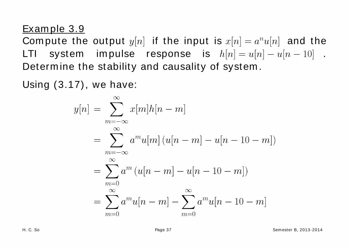
Example 3.9 Compute the output if the input is and the LTI system impulse response is . Determine the stability and causality of system.

Using (3.17), we have:


Let and such that . By employing a change of variable, is expressed as

Since for , for . For , is:

That is,


Similarly, is:

Since for , for . For , is:

That is,


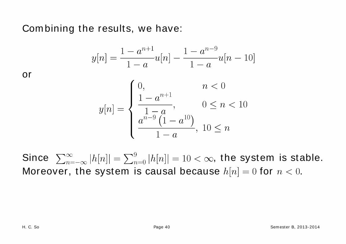
Combining the results, we have:

or

Since , the system is stable. Moreover, the system is causal because for .


Example 3.10 Determine where and are

and

We use the MATLAB command conv to compute the convolution of finite-length sequences: n=0:3; x=n.^2+1; h=n+1; y=conv(x,h) H. C. So Page 41 Semester B, 2013-2014

The results are y = 1 4 12 30 43 50 40 As the default starting time indices in both h and x are 1, we need to determine the appropriate time index for y The correct index can be obtained by computing one value of , say, :


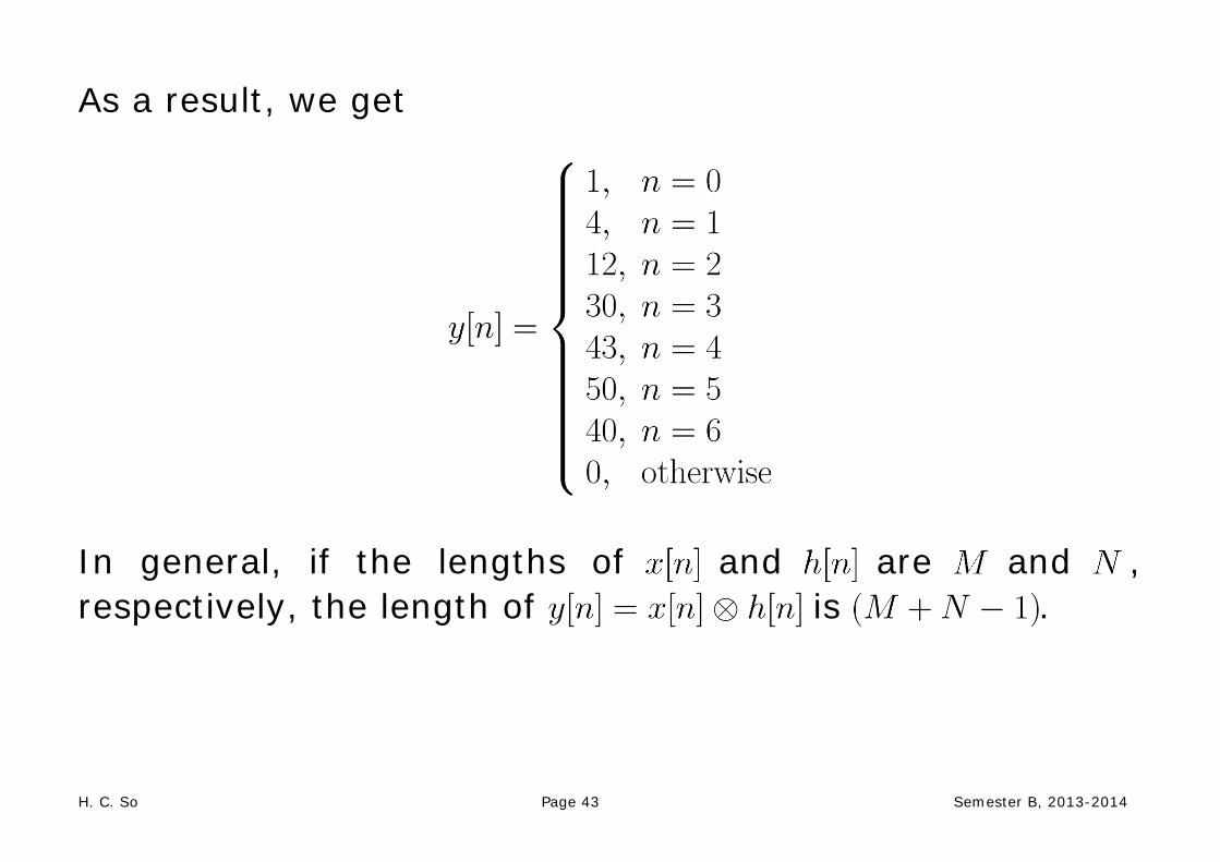
As a result, we get

In general, if the lengths of and are and , respectively, the length of is .


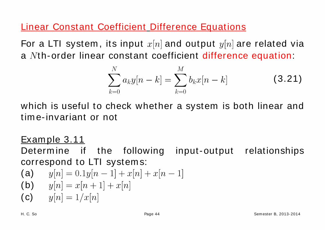
Linear Constant Coefficient Difference Equations

For a LTI system, its input and output are related via a th-order linear constant coefficient difference equation:

(3.21)

which is useful to check whether a system is both linear and time-invariant or not Example 3.11 Determine if the following input-output relationships correspond to LTI systems: (a) (b) (c) H. C. So Page 44 Semester B, 2013-2014

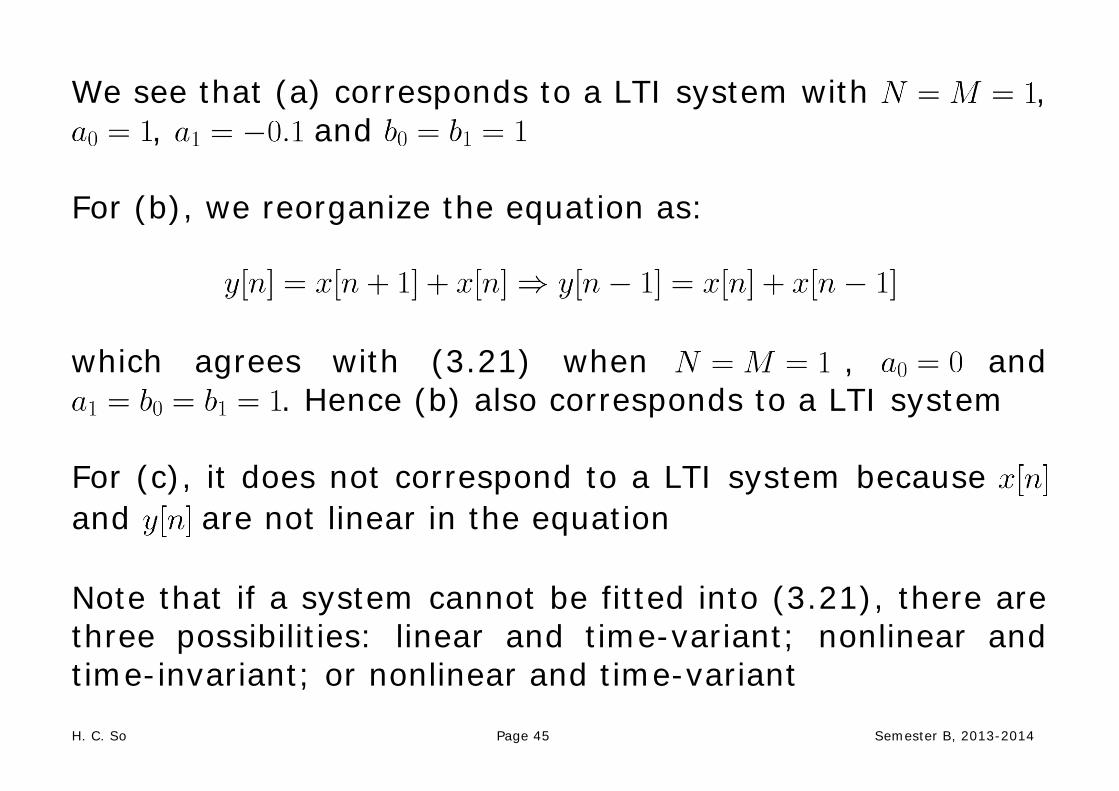
We see that (a) corresponds to a LTI system with , , and

For (b), we reorganize the equation as:

which agrees with (3.21) when , and

. Hence (b) also corresponds to a LTI system For (c), it does not correspond to a LTI system because and are not linear in the equation Note that if a system cannot be fitted into (3.21), there are three possibilities: linear and time-variant; nonlinear and time-invariant; or nonlinear and time-variant


Example 3.12 Compute the impulse response for a LTI system which is characterized by the following difference equation:

Expanding (3.17) as

we can easily deduce that only and are nonzero. That is, the impulse response is:


The difference equation is also useful to generate the system output and input. Assuming that , is computed as:

(3.22)

Assuming that , can be obtained from:

(3.23)


Example 3.13 Given a LTI system with difference equation of

, compute the system output for with an input of . It is assumed

that . The MATLAB code is: N=50; %data length is N+1 y(1)=1; %compute y[0], only x[n] is nonzero for n=2:N+1 y(n)=0.5*y(n-1)+2; %compute y[1],y[2],…,y[50]

%x[n]=x[n-1]=1 for n>=1 end n=[0:N]; %set time axis stem(n,y); H. C. So Page 48 Semester B, 2013-2014

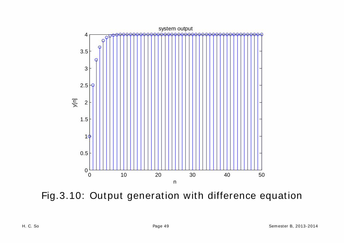
0 10 20 30 40 500

0.5

1

1.5

2

2.5

3

3.5

4

n

y[n]

system output

Fig.3.10: Output generation with difference equation


Alternatively, we can use the MATLAB command filter by rewriting the equation as:

The corresponding MATLAB code is:

x=ones(1,51); %define input a=[1,-0.5]; %define vector of a_k b=[1,1]; %define vector of b_k y=filter(b,a,x); %produce output stem(0:length(y)-1,y)

The x is the input which has a value of 1 for , while a and b are vectors which contain and , respectively.

The MATLAB programs for this example are provided as ex3_13.m and ex3_13_2.m.


Documents

Discrete-Time Signals and Systems - Department of EEhcso/ee4219_3.pdf · Discrete-Time Signals and Systems. ... Understanding deterministic and random discrete-time signals and ability