Stalking the “Efficient Price” in Market Microstructure Specifications:

An Overview

Joel Hasbrouck

May 25, 2000 This version: June 21, 2000

Preliminary Draft Not for Quotation

Comments Welcome

Professor of Finance Stern School of Business New York University Suite 9-190 Mail Code 0268 44 West Fourth St. New York, NY 10012-1126

Tel: (212) 998-0310 Fax: (212) 995–4901 E-mail: jhasbrou@stern.nyu.edu

The most recent version of this paper and Matlab programs used in the analysis are

available at http://www.stern.nyu.edu/~jhasbrou

Stalking the “Efficient Price” in Market Microstructure Specifications:

An Overview

Abstract

The principle that revisions to the expectation of a security’s value should be

unforecastable identifies this expectation as a martingale. When price changes can

plausibly be assumed covariance stationary, this in turn motivates interest in the random

walk. In the presence of the market frictions featured in many microstructure models,

however, this expectation does not invariably coincide with observed security prices such

as trades and quotes. Accordingly, the random walk becomes an implicit, unobserved

component. This paper is an overview of econometric approaches to characterizing this

important component in single- and multiple-price applications.

Page 3

1. Introduction

In modeling security price dynamics, the martingale and its statistically expedient

variant, the random walk, have long figured prominently. Historically, the martingale

and random-walk models have usually been employed in security price studies at daily

and longer horizons. At long horizons, it is common (and often appropriate) to ignore the

finer details of the trading process. A random-walk specification estimated directly for

monthly closing stock prices, for example, is a reasonable point of reference or departure.

Over shorter intervals (e.g., trade-to-trade), however, market frictions and effects

attributable to trading process often introduce short-term, transient effects. The most

prominent example is perhaps the “bounce” arising from trades that randomly occur at

the bid or ask prices. Such effects introduce dependencies into the price dynamics. In

consequence the unadorned random walk is no longer an attractive or reasonable

specification.

Despite this, it is grossly incorrect to conclude that martingales have no further

relevance. Traders still rely on their beliefs about what the security is worth. In virtually

all microstructure models, the expectation of terminal security value conditional on

current information plays a crucial role. Broadly speaking, when the information set is

increasingly refined (“a filtration”) this (indeed, any) sequence of conditional

expectations is a martingale. In recognition of this, many structural microstructure

models are formed by adding trading-related effects to a random walk that is simply

called the “efficient price”. Consistent with this usage, the present paper will use the

term “efficient price” to refer to a martingale expectation of future (perhaps terminal)

prices.

When we introduce microstructure effects into a price model, we break the

identity between the observed price and the underlying expected-value martingale. To

address this difficulty, we need econometric approaches that allow us to characterize this

Page 4

structural, implicit, unobserved martingale. This note seeks to summarize and review

such approaches.1

These approaches are mostly drawn from the econometric literature that focuses

on macroeconomic time series. Statistical theorems and proofs are valid, of course,

whether t indexes years or seconds. Nevertheless, model specifications and identification

restrictions are often highly dependent on the assumed underlying structural economic

model. Restrictions that are reasonable for macroeconomic time series might well be

objectionable in analyses of microstructure data (and vice versa). There are no one-size-

fits-all statistical models.

2. Random walk decompositions

a. Martingales in market microstructure

In the usual theoretical models, the martingale property of security prices is a

manifestation of “market efficiency”, a property of the dynamic economic equilibrium.

Although the original formulations relied on frictionless perfect market assumptions, the

martingale property is robust to certain imperfections that fall under the microstructure

purview. Perhaps most importantly, asymmetric information does not inevitably cause

non-martingale behavior (Easley and O'Hara (1987); Glosten and Milgrom (1985); Kyle

(1985)).

The effects of fixed transaction costs, inventory control and price discreteness are

more complicated. In the Roll (1984) model, for example, “bid-ask bounce” leads to

transaction price changes that are negatively dependent. The model is typical, however,

in that long-run changes in transaction prices are dominated by an implicit martingale, the

midpoint of the bid and ask quotes (which is, in Roll’s application, unobserved). The

1 Hamilton (1994) is a textbook reference for most of the standard time-series results

invoked in this paper. Hasbrouck (1996) discusses related microstructure applications of

this material.

Page 5

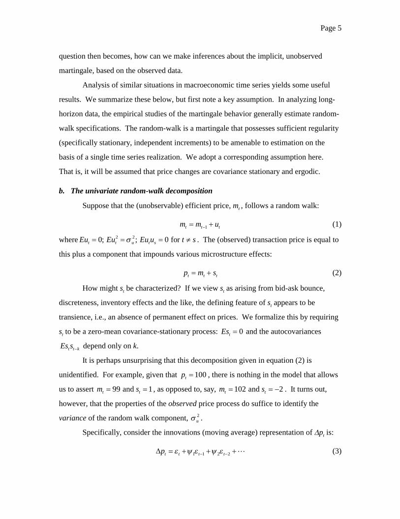
question then becomes, how can we make inferences about the implicit, unobserved

martingale, based on the observed data.

Analysis of similar situations in macroeconomic time series yields some useful

results. We summarize these below, but first note a key assumption. In analyzing long-

horizon data, the empirical studies of the martingale behavior generally estimate random-

walk specifications. The random-walk is a martingale that possesses sufficient regularity

(specifically stationary, independent increments) to be amenable to estimation on the

basis of a single time series realization. We adopt a corresponding assumption here.

That is, it will be assumed that price changes are covariance stationary and ergodic.

b. The univariate random-walk decomposition

Suppose that the (unobservable) efficient price, mt , follows a random walk:

1t t tm m u−= + (1)

where 2 20; ; 0 for t t u t sEu Eu Eu u t sσ= = = ≠ . The (observed) transaction price is equal to

this plus a component that impounds various microstructure effects:

t t tp m s= + (2)

How might st be characterized? If we view st as arising from bid-ask bounce,

discreteness, inventory effects and the like, the defining feature of st appears to be

transience, i.e., an absence of permanent effect on prices. We formalize this by requiring

st to be a zero-mean covariance-stationary process: 0tEs = and the autocovariances

t t kEs s − depend only on k.

It is perhaps unsurprising that this decomposition given in equation (2) is

unidentified. For example, given that 100tp = , there is nothing in the model that allows

us to assert 99 and 1t tm s= = , as opposed to, say, 102 and 2t tm s= = − . It turns out,

however, that the properties of the observed price process do suffice to identify the

variance of the random walk component, 2uσ .

Specifically, consider the innovations (moving average) representation of ∆pt is:

1 1 2 2t t t tp ε ψ ε ψ ε− −∆ = + + +! (3)

Page 6

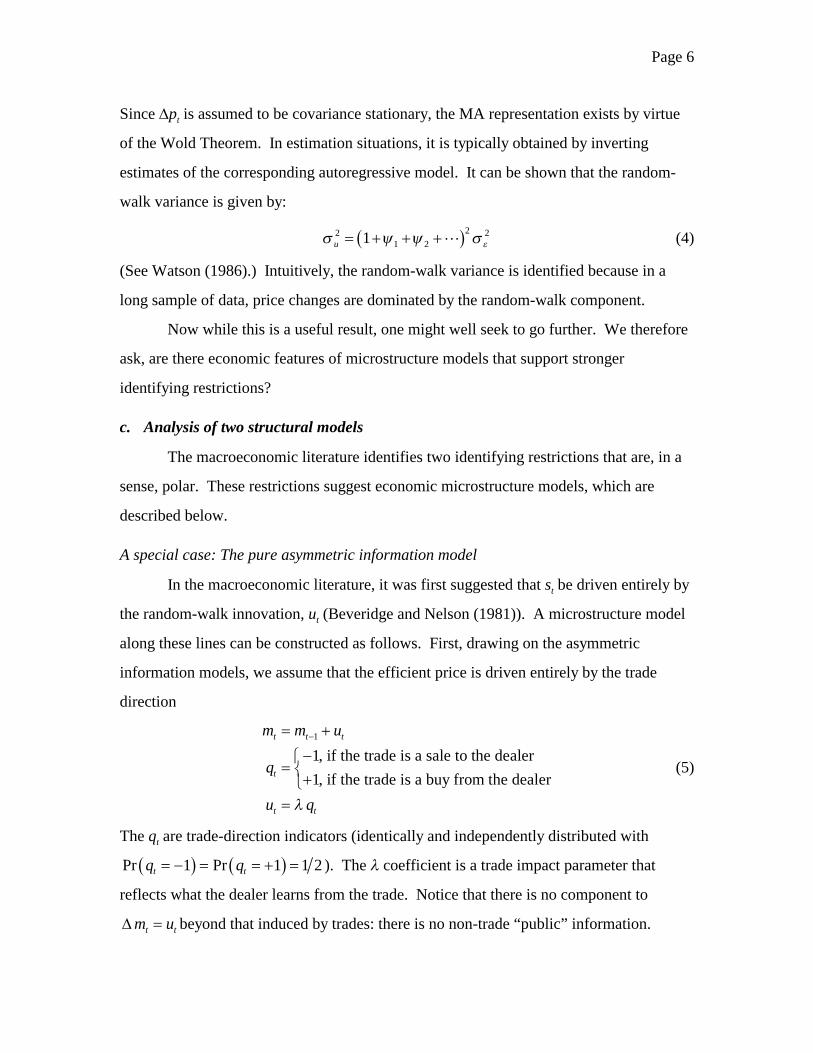
Since ∆pt is assumed to be covariance stationary, the MA representation exists by virtue

of the Wold Theorem. In estimation situations, it is typically obtained by inverting

estimates of the corresponding autoregressive model. It can be shown that the random-

walk variance is given by:

( )22 21 21u εσ ψ ψ σ= + + +! (4)

(See Watson (1986).) Intuitively, the random-walk variance is identified because in a

long sample of data, price changes are dominated by the random-walk component.

Now while this is a useful result, one might well seek to go further. We therefore

ask, are there economic features of microstructure models that support stronger

identifying restrictions?

c. Analysis of two structural models

The macroeconomic literature identifies two identifying restrictions that are, in a

sense, polar. These restrictions suggest economic microstructure models, which are

described below.

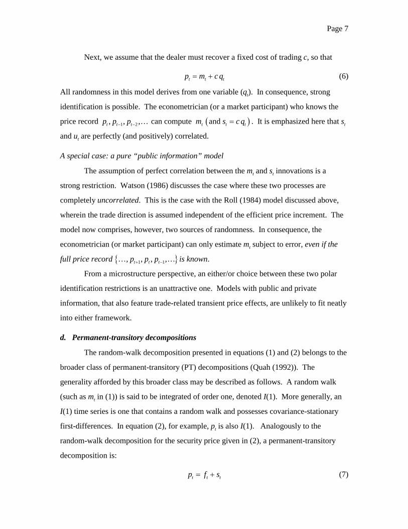
A special case: The pure asymmetric information model

In the macroeconomic literature, it was first suggested that st be driven entirely by

the random-walk innovation, ut (Beveridge and Nelson (1981)). A microstructure model

along these lines can be constructed as follows. First, drawing on the asymmetric

information models, we assume that the efficient price is driven entirely by the trade

direction

1

1, if the trade is a sale to the dealer1, if the trade is a buy from the dealer

t t t

t

t t

m m u

q

u qλ

−= +

−= +=

(5)

The qt are trade-direction indicators (identically and independently distributed with

( ) ( )Pr 1 Pr 1 1 2t tq q= − = = + = ). The λ coefficient is a trade impact parameter that

reflects what the dealer learns from the trade. Notice that there is no component to

t tm u∆ = beyond that induced by trades: there is no non-trade “public” information.

Page 7

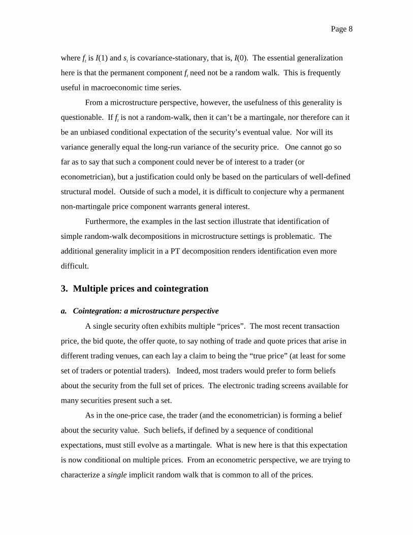
Next, we assume that the dealer must recover a fixed cost of trading c, so that

t t tp m c q= + (6)

All randomness in this model derives from one variable (qt). In consequence, strong

identification is possible. The econometrician (or a market participant) who knows the

price record 1 2, , ,t t tp p p− − … can compute mt ( )and t ts c q= . It is emphasized here that st

and ut are perfectly (and positively) correlated.

A special case: a pure “public information” model

The assumption of perfect correlation between the mt and st innovations is a

strong restriction. Watson (1986) discusses the case where these two processes are

completely uncorrelated. This is the case with the Roll (1984) model discussed above,

wherein the trade direction is assumed independent of the efficient price increment. The

model now comprises, however, two sources of randomness. In consequence, the

econometrician (or market participant) can only estimate mt subject to error, even if the

full price record 1 1, , , ,t t tp p p+ −… … is known.

From a microstructure perspective, an either/or choice between these two polar

identification restrictions is an unattractive one. Models with public and private

information, that also feature trade-related transient price effects, are unlikely to fit neatly

into either framework.

d. Permanent-transitory decompositions

The random-walk decomposition presented in equations (1) and (2) belongs to the

broader class of permanent-transitory (PT) decompositions (Quah (1992)). The

generality afforded by this broader class may be described as follows. A random walk

(such as mt in (1)) is said to be integrated of order one, denoted I(1). More generally, an

I(1) time series is one that contains a random walk and possesses covariance-stationary

first-differences. In equation (2), for example, pt is also I(1). Analogously to the

random-walk decomposition for the security price given in (2), a permanent-transitory

decomposition is:

t t tp f s= + (7)

Page 8

where ft is I(1) and st is covariance-stationary, that is, I(0). The essential generalization

here is that the permanent component ft need not be a random walk. This is frequently

useful in macroeconomic time series.

From a microstructure perspective, however, the usefulness of this generality is

questionable. If ft is not a random-walk, then it can’t be a martingale, nor therefore can it

be an unbiased conditional expectation of the security’s eventual value. Nor will its

variance generally equal the long-run variance of the security price. One cannot go so

far as to say that such a component could never be of interest to a trader (or

econometrician), but a justification could only be based on the particulars of well-defined

structural model. Outside of such a model, it is difficult to conjecture why a permanent

non-martingale price component warrants general interest.

Furthermore, the examples in the last section illustrate that identification of

simple random-walk decompositions in microstructure settings is problematic. The

additional generality implicit in a PT decomposition renders identification even more

difficult.

3. Multiple prices and cointegration

a. Cointegration: a microstructure perspective

A single security often exhibits multiple “prices”. The most recent transaction

price, the bid quote, the offer quote, to say nothing of trade and quote prices that arise in

different trading venues, can each lay a claim to being the “true price” (at least for some

set of traders or potential traders). Indeed, most traders would prefer to form beliefs

about the security from the full set of prices. The electronic trading screens available for

many securities present such a set.

As in the one-price case, the trader (and the econometrician) is forming a belief

about the security value. Such beliefs, if defined by a sequence of conditional

expectations, must still evolve as a martingale. What is new here is that this expectation

is now conditional on multiple prices. From an econometric perspective, we are trying to

characterize a single implicit random walk that is common to all of the prices.

Page 9

A statistical model of the joint behavior of such a set of prices must reflect two

considerations. First, each price (considered individually) is I(1) (contains a random

walk). Second, pairs of prices are linked in the long run by arbitrage and/or equilibrium

relationships. Therefore, any two prices will not arbitrarily diverge over time. These

considerations imply that the set of prices embodies a single long-term component.

Formally, we say that the set of prices is cointegrated.

Cointegration is related to, but quite distinct from, correlation. The daily high-

water mark of the Hudson River at 96th Street is highly correlated with the measurement

taken at 14th Street. But the two series of measurements are not cointegrated because

neither is individually integrated. (Neither measure will tend to wander off over time

without bound.) Moreover, cointegration is a stronger restriction than correlation. The

daily price changes of Ford and GM are positively correlated due to common industry

effects. But there are no obvious equilibrium or arbitrage relationships that tie the two

firms together: one might eventually go bankrupt while the other thrives. On the other

hand, the bid and offer quotes for GM are almost certainly cointegrated. The difference

between these two prices (the ask less the bid) is the spread. The spread cannot go

negative or explode without bound (given any reasonable economic model of competitive

liquidity provision).

The analysis of macroeconomic time series has yielded many useful results in the

specification and estimation of cointegrated models. Relative to macro applications,

however, microstructure cointegrated models are usually much simpler. Macroeconomic

analyses are complicated because the precise nature of the cointegrating relations is

unknown. In the long run, for example, the proportion of consumption to national

income is likely to be stationary. (That is, the log of consumption and the log of income

are cointegrated.) But since there is no obvious way to specify the proportion a priori, it

must be estimated. Microstructure models are more precise. Although the price of GM

on the New York and Boston Exchanges might differ at any given time, it is sensible to

assume that this difference is stationary. Formally, this identifies a basis for the

cointegrating vectors.

Page 10

b. A dual market example

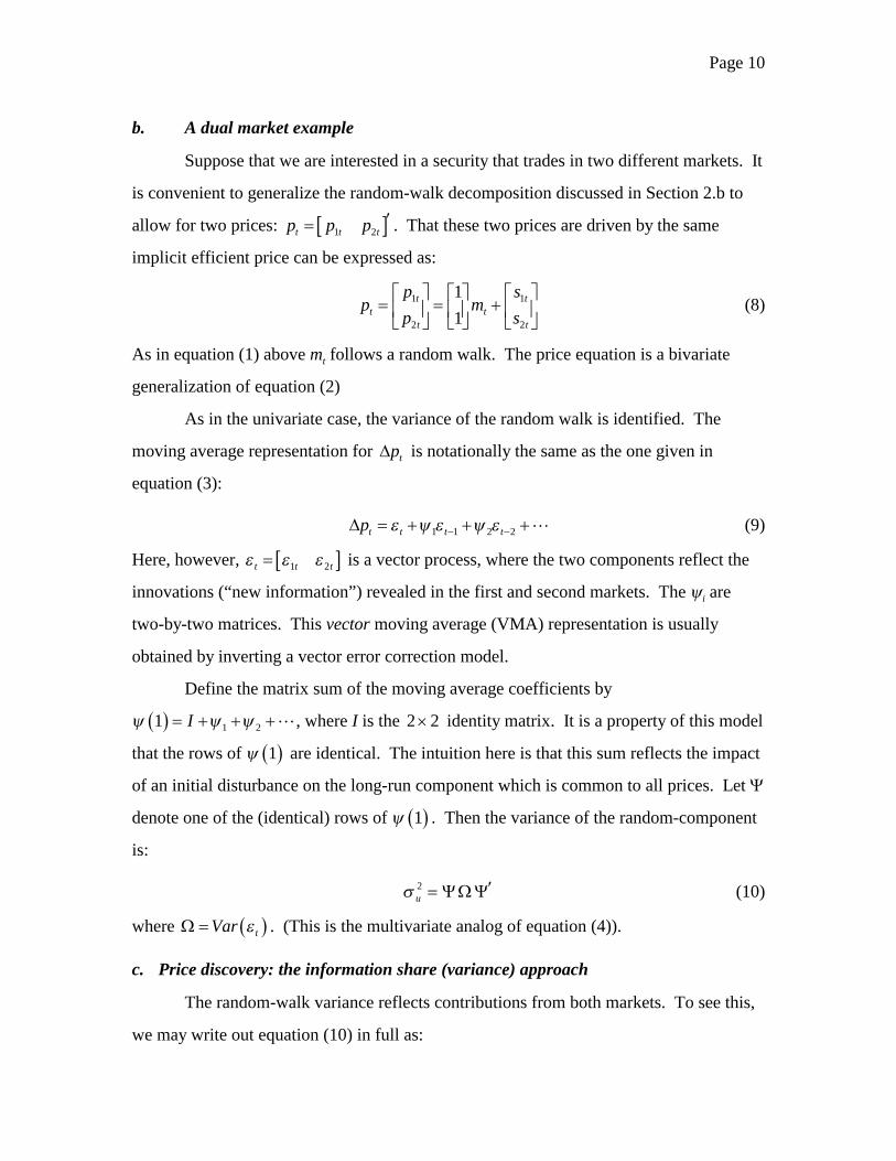
Suppose that we are interested in a security that trades in two different markets. It

is convenient to generalize the random-walk decomposition discussed in Section 2.b to

allow for two prices: [ ]1 2t t tp p p ′= . That these two prices are driven by the same

implicit efficient price can be expressed as:

1 1

2 2

11

t tt t

t t

p sp m

p s

= = +

(8)

As in equation (1) above mt follows a random walk. The price equation is a bivariate

generalization of equation (2)

As in the univariate case, the variance of the random walk is identified. The

moving average representation for tp∆ is notationally the same as the one given in

equation (3):

1 1 2 2t t t tp ε ψ ε ψ ε− −∆ = + + +! (9)

Here, however, [ ]1 2t t tε ε ε= is a vector process, where the two components reflect the

innovations (“new information”) revealed in the first and second markets. The ψi are

two-by-two matrices. This vector moving average (VMA) representation is usually

obtained by inverting a vector error correction model.

Define the matrix sum of the moving average coefficients by

( ) 1 21 Iψ ψ ψ= + + +! , where I is the 2 2× identity matrix. It is a property of this model

that the rows of ( )1ψ are identical. The intuition here is that this sum reflects the impact

of an initial disturbance on the long-run component which is common to all prices. Let Ψ

denote one of the (identical) rows of ( )1ψ . Then the variance of the random-component

is:

2uσ ′= ΨΩΨ (10)

where ( )tVar εΩ = . (This is the multivariate analog of equation (4)).

c. Price discovery: the information share (variance) approach

The random-walk variance reflects contributions from both markets. To see this,

we may write out equation (10) in full as:

Page 11

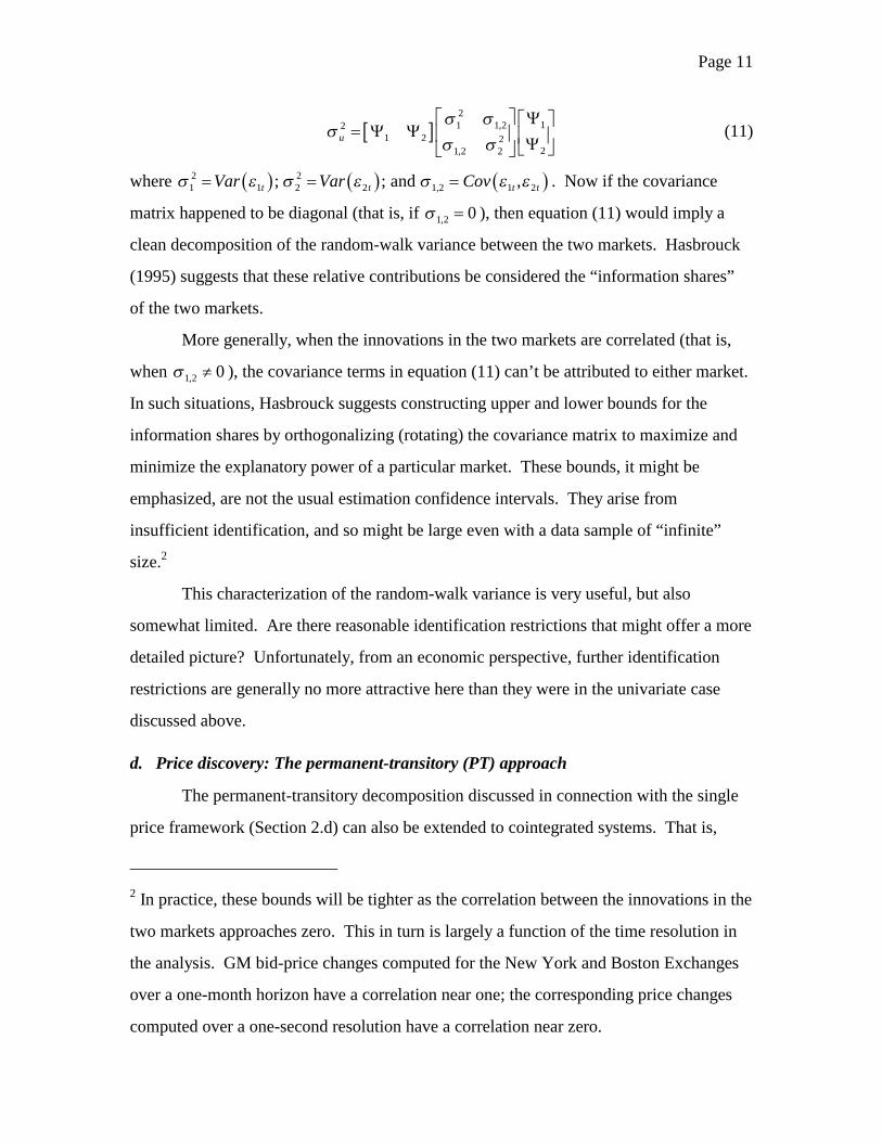
[ ]2

11 1,221 2 2

21,2 2u

σ σσ

σ σ Ψ

= Ψ Ψ Ψ (11)

where ( ) ( ) ( )2 21 1 2 2 1,2 1 2; ; and ,t t t tVar Var Covσ ε σ ε σ ε ε= = = . Now if the covariance

matrix happened to be diagonal (that is, if 1,2 0σ = ), then equation (11) would imply a

clean decomposition of the random-walk variance between the two markets. Hasbrouck

(1995) suggests that these relative contributions be considered the “information shares”

of the two markets.

More generally, when the innovations in the two markets are correlated (that is,

when 1,2 0σ ≠ ), the covariance terms in equation (11) can’t be attributed to either market.

In such situations, Hasbrouck suggests constructing upper and lower bounds for the

information shares by orthogonalizing (rotating) the covariance matrix to maximize and

minimize the explanatory power of a particular market. These bounds, it might be

emphasized, are not the usual estimation confidence intervals. They arise from

insufficient identification, and so might be large even with a data sample of “infinite”

size.2

This characterization of the random-walk variance is very useful, but also

somewhat limited. Are there reasonable identification restrictions that might offer a more

detailed picture? Unfortunately, from an economic perspective, further identification

restrictions are generally no more attractive here than they were in the univariate case

discussed above.

d. Price discovery: The permanent-transitory (PT) approach

The permanent-transitory decomposition discussed in connection with the single

price framework (Section 2.d) can also be extended to cointegrated systems. That is,

2 In practice, these bounds will be tighter as the correlation between the innovations in the

two markets approaches zero. This in turn is largely a function of the time resolution in

the analysis. GM bid-price changes computed for the New York and Boston Exchanges

over a one-month horizon have a correlation near one; the corresponding price changes

computed over a one-second resolution have a correlation near zero.

Page 12

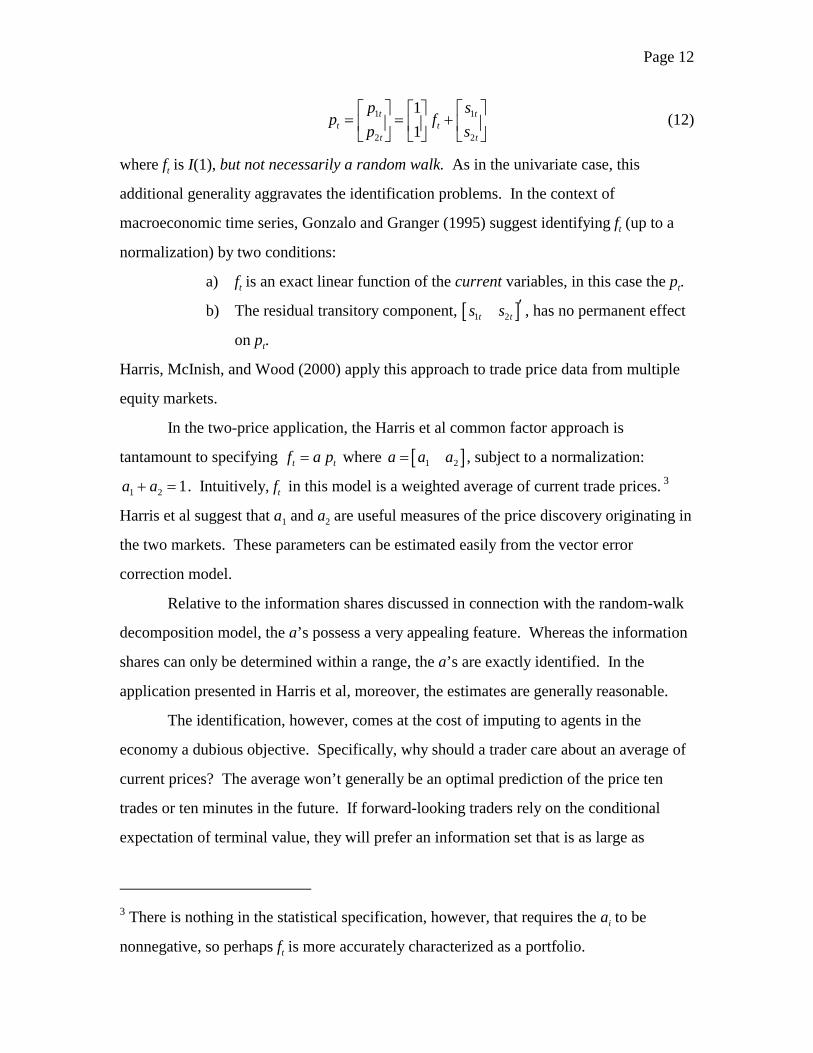
1 1

2 2

11

t tt t

t t

p sp f

p s

= = +

(12)

where ft is I(1), but not necessarily a random walk. As in the univariate case, this

additional generality aggravates the identification problems. In the context of

macroeconomic time series, Gonzalo and Granger (1995) suggest identifying ft (up to a

normalization) by two conditions:

a) ft is an exact linear function of the current variables, in this case the pt.

b) The residual transitory component, [ ]1 2t ts s ′ , has no permanent effect

on pt.

Harris, McInish, and Wood (2000) apply this approach to trade price data from multiple

equity markets.

In the two-price application, the Harris et al common factor approach is

tantamount to specifying t tf a p= where [ ]1 2a a a= , subject to a normalization:

1 2 1a a+ = . Intuitively, ft in this model is a weighted average of current trade prices. 3

Harris et al suggest that a1 and a2 are useful measures of the price discovery originating in

the two markets. These parameters can be estimated easily from the vector error

correction model.

Relative to the information shares discussed in connection with the random-walk

decomposition model, the a’s possess a very appealing feature. Whereas the information

shares can only be determined within a range, the a’s are exactly identified. In the

application presented in Harris et al, moreover, the estimates are generally reasonable.

The identification, however, comes at the cost of imputing to agents in the

economy a dubious objective. Specifically, why should a trader care about an average of

current prices? The average won’t generally be an optimal prediction of the price ten

trades or ten minutes in the future. If forward-looking traders rely on the conditional

expectation of terminal value, they will prefer an information set that is as large as

3 There is nothing in the statistical specification, however, that requires the ai to be

nonnegative, so perhaps ft is more accurately characterized as a portfolio.

Page 13

possible. If past prices contain useful information, why should they be excluded from the

conditioning set?

e. Information-share and common-factor measures of price discovery: a comparison

The relative merits of the information share (IS) and permanent-transitory (PT)

measures of price discovery might be summarized as follows. The information shares

arise from a random-walk decomposition subject to minimal identification restrictions.

The implicit random walk, being a martingale, is consistent with rational updating of

conditional expectations. Estimates of the information shares, however, can be

determined only within bounds that are likely to be uncomfortably large in many

applications. The permanent factor coefficients (the a) in the PT approach, on the other

hand, may be estimated much more precisely. Their economic justification, however,

rests on the presumption that the representative trader’s objective is an average of current

prices.

The contrast has to this point, been made at an abstract level of economic and

econometric principle. The reader might well be wondering if material differences

between the two approaches are likely to arise in practice. To answer this question, I

consider the implications of both approaches for three simple structural models. That is,

I consider the behavior of these specifications in situations when the structural models are

known and the estimation procedures are applied to data generated by artificial, but

nonetheless plausible, economic models.

Price discovery example I: A two-market “Roll” model.

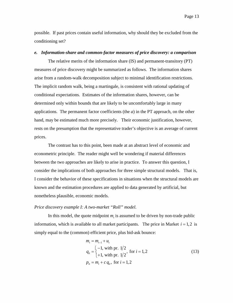
In this model, the quote midpoint mt is assumed to be driven by non-trade public

information, which is available to all market participants. The price in Market 1,2i = is

simply equal to the (common) efficient price, plus bid-ask bounce:

1

1, with pr. 1 2, for 1,2

1, with pr. 1 2, for 1,2

t t t

it

it t it

m m u

q i

p m c q i

−= +

−= =+= + =

(13)

Page 14

I assume that 1 2, ,t t tu q q are mutually uncorrelated. The two markets in this model are

(statistically) identical. This symmetry suggests that, in a structural sense, neither market

should dominate. Any sensible attributions of price discovery should either be

indeterminate or of equal share (0.5). With parameter values 1 and 1uc σ= = , I

generated 100,000 observations, and analyzed the data according the PT and IS

approaches.

Table 1 summarizes the results. The PT approach determines an attribution of

price discovery to Market 1 that is (to reported precision) identical to the “correct” (that

is, structural) value, 0.5. The bounds implied by the information share approach certainly

contain this value, but the range is a wide one (0.21, 0.79).

All else equal, one is drawn to the PT approach here because it appears to arrive

at the correct value with little uncertainty. There are, however, some drawbacks to this

attribution. The statistical properties of the PT common price factor, in this case

1 20.5 0.5t t tf p p= + differ dramatically from those of the structural efficient price. With

the parameter values used here, ( ) ( )211 and , 0t u t tVar m Corr m mσ −∆ = = ∆ ∆ = . In the

simulated data, however, ( ) 2.00tVar f∆ = and ( )1, 0.25t tCorr f f −∆ ∆ = − . Thus, an

analysis that takes ft as a proxy for the structural efficient price will grossly overestimate

volatility and autocorrelation. Under the IS approach, however, the estimated variance of

the common price factor (the random walk) component is 1.01, with first-order

autocorrelation that is zero (by construction).

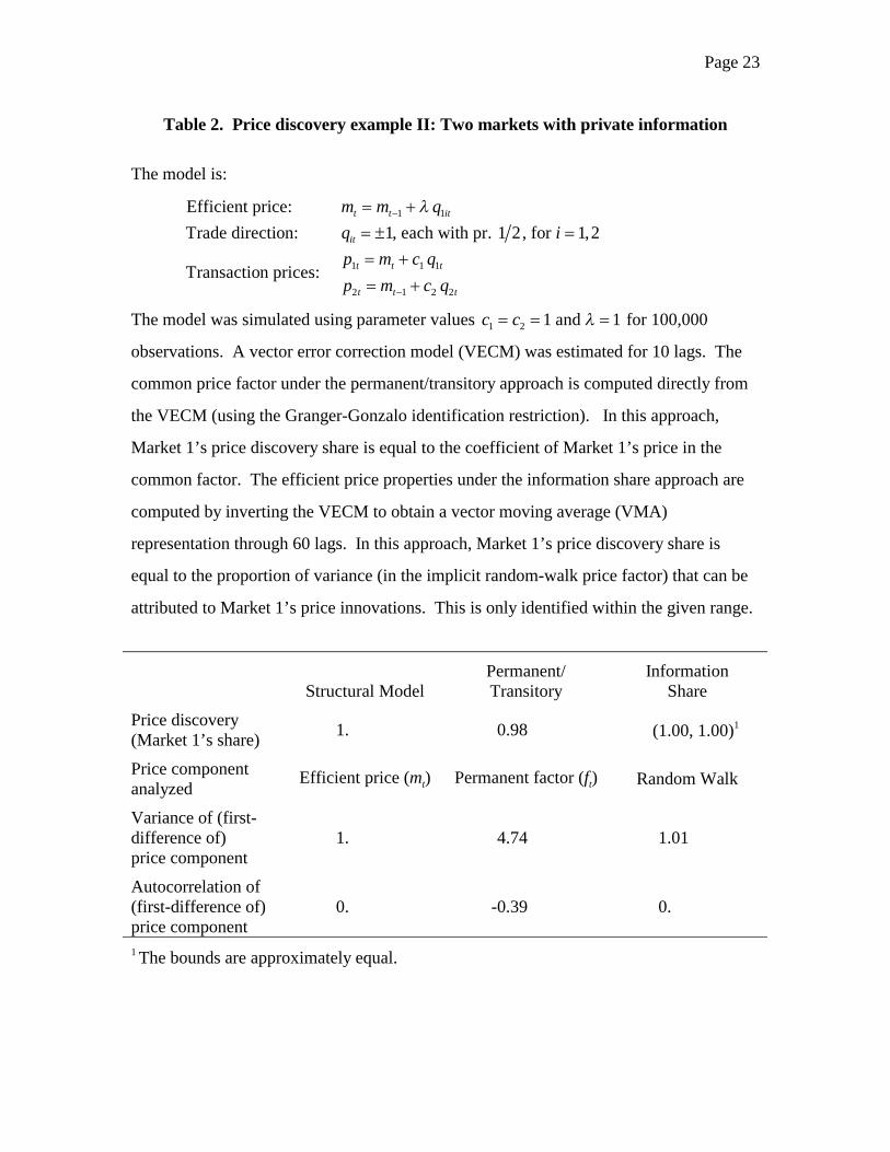
Price discovery example II: Two markets with private information.

Suppose that Market 1 is identical to the asymmetric information market

considered in Section 2.c. That is, the quote midpoint mt is driven purely by Market 1’s

trades:

1 1t t tm m qλ−= + (14)

The transaction price in this market is

1 1 1t t tp m c q= + .

Market 2 is the derivative (satellite) market, with trade prices given by

Page 15

2 1 2 2t t tp m c q−= + .

Note that Market 2 relies on the lagged (stale) value of mt. Thus, from a structural

viewpoint, it is clear that all price discovery occurs in the first market. For parameter

values 1 2 1c c= = and 1λ = , I simulated and analyzed 100,000 observations.

Table 2 summarizes the results. As in the previous example, the PT approach

attributes nearly all of the price discovery to the Market 1 (the structurally correct

answer). The IS approach also makes this determination. In contrast to the last example,

the bounds of the price discovery share are very tight. (This is a consequence of there

being only one source of randomness in the Market 1 price. Because the 1tp dynamics

are driven entirely by 1tq , mt can be recovered exactly from current and past prices.)

Although the PT and IS approaches give similar determinations of price

discovery, the behavior of the common price factors differs strongly (as in the last

example). The random-walk component in the IS approach has moments that are very

similar to those of the efficient price. The PT price factor ft has a variance that is more

than four times as large as that of the efficient price, however. The factor also exhibits

strong negative autocorrelation.

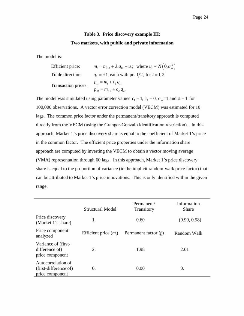
Price discovery example III: Two markets with public and private information.

Example III combines features of Examples I and II. The quote midpoint mt is

driven by Market 1’s trades and a non-trade (“public information”) component:

( )21 1 where ~ 0,t t t t t um m q u u Nλ σ−= + + (15)

The transaction price in this market is

1 1 1t t tp m c q= + .

As in example II, Market 2 is the derivative (satellite) market, with trade prices based

stale (lagged) information.

2 1 2 2t t tp m c q−= + .

Once again, Market 1 is in a structural sense, the clear leader.

The parameter values used for the simulations were 1 1c = , 2 0c = and 1λ = .

Page 16

A supporting economic story here might be that 1 2c c> because the costs of market-

making (including monitoring and regulatory systems) in an environment with informed

trading are larger than the costs of a passive system. Market 2 crosses trades cheaply

(costlessly) at stale prices.4 I simulated and analyzed 100,000 observations.

Table 3 reports the results. The PT approach attributes 60% of the price

discovery to Market 1; the bounds of the IS attribution are (90%, 98%). Thus (up to an

estimation error) the IS bounds contain the correct value. The PT attribution is a

substantial underestimate, and also lies below the lower bound of the IS range. As in the

earlier examples, the statistical properties of the random-walk component in the IS

approach are quite close to those of the structural efficient price. In contrast with the

earlier examples, this also characterizes the PT common factor.

Summary

The examples studied here cover a range of structural models: one in which all

information is public; one in which all information is private (trade-related); and one with

a mix of public and private information.

In the analysis of these examples, neither the PT nor the IS approaches always

arrives precisely at the structurally-correct determination. The bounds generated by the

IS approach usually contain (up to estimation error) the true value. This cannot be said of

the PT approach, which may be quite misleading (as in example III).

It might be alleged in favor of the PT approach that it sometimes achieves a

precise identification when the IS bounds are vague (as in example I). But the price

factor so constructed in this situation is substantially more volatile and autocorrelated

than the structural efficient price. This raises questions about the extent to which the PT

factor approximates the structural efficient price.

4 In the analysis of example II, the parameterization was 1 2 1c c= = . Setting 1 1c = and

2 0c = in Example II yields a system that is noninvertible, and therefore cannot be

estimated by a VECM.

Page 17

On balance, therefore, the IS approach appears to support more reliable inference.

As long as the price component of interest is presumed to follow a random walk, the IS

analysis offers the most accurate characterization. The random-walk restriction on the

efficient price is motivated by the economic logic that this component should behave as a

martingale. It might well be the case that other microstructure considerations motivate

interest in non-random-walk price components. But absent such structural economic

considerations, the rationale for alternative statistical restrictions (as in the PT approach)

is, in microstructure applications, unclear.

4. Multiple markets with different trading frequencies

The discussion of the multiple-market models in the previous section made no

note of a particular feature that greatly simplified the analysis. Specifically, the data

record contained contemporaneously-determined prices for each market for each time t.

This feature is unfortunately quite problematic in practice. Transaction frequency often

differs dramatically across the various markets in which a security is traded. Obtaining a

multivariate transaction price series in which the component prices are determined

approximately contemporaneously, therefore, requires thinning the data set.

Thinning is not an innocuous procedure. By discarding prices established in the

higher-frequency market that are not close in time to trades in the low-frequency market,

the analyst suppresses any economic value these “intermediate” prices might have.

Furthermore, inferences about price discovery that includes these intermediate times

might be reversed in an analysis that focuses only on times with coincident (or nearly

coincident) prices. Two examples illustrate these points.

Data thinning example I

Suppose that the efficient price evolves as a random walk,

1t t tm m u−= + , (16)

where t indexes “minutes”. Market 1 (the “high-frequency market”) has a trade every

minute at price 1t tp m= . Market 2 (the “low-frequency market”) has a trade every 100

minutes:

Page 18

2

if mod( ,100) 0, otherwise

tt

m tp

Undefined=

=

(17)

From a structural perspective, all the price discovery at intermediate times (that is, times

at which ( )mod ,100 0t ≠ ) is occurring in Market 1. If we thin the data set to the

“endpoint” times 100 for 1,2,t i i= = …, then the two markets will appear to be

informationally equivalent.

Data thinning example II:

This example, although perhaps extreme, illustrates the problem with relying

solely on endpoint prices. We extend the previous example to “penalize” Market 1 as

follows:

( )11

, if mod ,100 0, otherwise

tt

t

m tp

m− =

=

(18)

That is, Market 1 still performs all of the price discovery during intermediate times, but

uses stale prices at the endpoints. Viewed over all t, Market 1 performs 99% of the price

discovery. But viewed solely from the endpoints, Market 1 appears completely

redundant.5

Thinning: a summary

Market data are not always conveniently timed, and it is probably too strong a

pronouncement to assert that thinning is never justified. But the above examples should

introduce an element of doubt or qualification to the practice. Thinning is essentially

censoring, and price patterns that clearly characterize a full data record may be obscured

or reversed in a censored sample.

Moreover, the examples featured exogenous trading occurrences. If trade

occurrence is endogenous to the information process, the possibilities of misleading

inference increase further. Suppose, for example, that in reaction to new information,

5 That is, a time-series analysis of endpoint price changes would (in a sufficiently large

sample) find Granger-Sims causality running from Market 2 to Market 1, but not the

reverse.

Page 19

traders in the satellite market refrain from transacting until prices in the dominant market

have “settled down”.

5. Conclusions

From an econometric perspective, market frictions such as bid-ask bounce,

discreteness, inventory control, etc., generally introduce transient components into

security price processes. In the presence of such components, these prices aren’t

martingales. The martingale still figures prominently in the analysis because this

property characterizes a sequence of conditional expectations, such as those formed by

traders regarding a security’s ultimate value. This sequence of expectations is

unobserved, however, and so the martingale must be regarded as an implicit one.

With this perspective, the present paper summarizes econometric approaches to

characterizing the unobserved random walk component of a security price. These

techniques mostly originated in the analysis of macroeconomic time series. While the

basic results are invariant to time scale, however, there are structural economic features

of microstructure settings that must be taken into account.

Thus, decompositions that characterize the random-walk component implicit in a

price series with covariance-stationary first differences play a prominent role. It is

generally possible to compute the variance of this component, and to characterize

contributions to this variance. When the supporting data comprise prices of the same

security from multiple markets, these techniques support qualified attributions of price

discovery.

Stronger results, however, such as determining precisely the location of the

implicit random-walk component at a given time, rely on identification restrictions that

are not plausible in microstructure settings, irrespective of their merits in macroeconomic

applications. Moreover, general permanent-transitory decompositions used in

macroeconomics, when applied to microstructure price data, characterize non-martingale

factors. While non-martingale factors might be of interest in a particular structural

Page 20

model, they are poor proxies for optimally formed and updated expectations of security

value.

The paper considers the attribution of price discovery in multiple markets using

simulated data from simple structural models of trading. The analysis contrasts the

information share approach discussed in Hasbrouck (1995), in which the price component

of interest is forced to be a random walk, with the approach suggested by Harris,

McInish, and Wood (2000), in which the price component is permanent in the sense of

Gonzalo and Granger (1995). Although the latter approach can sometimes appear to

offer greater precision, the information share computation is more reliable.

Finally, multiple-market analyses often compare venues with differing trading

frequencies. The desire for contemporaneously-determined prices motivates a thinning

of the data, to include only those times (or small time windows) in which trades occurred

in all markets. This paper shows that this censoring can drastically affect the inferences

concerning price discovery. Clear patterns of price leadership in the full data set can be

obscured or even reversed by the censoring.

6. References

Beveridge, S., Nelson, C. R., 1981. A new approach to the decomposition of economic

time series into permanent and transitory components with particular attention to

the measurement of the 'business cycle'. Journal of Monetary Economics 7, 151-

174.

Easley, D., O'Hara, M., 1987. Price, trade size, and information in securities markets.

Journal of Financial Economics 19, 69-90.

Glosten, L. R., Milgrom, P. R., 1985. Bid, ask, and transaction prices in a specialist

market with heterogeneously informed traders. Journal of Financial Economics

14, 71-100.

Gonzalo, J., Granger, C., 1995. Estimation of common long-memory components in

Page 21

cointegrated systems. Journal of Business and Economic Statistics 13, 27-35.

Hamilton, J.D., 1994. Time Series Analysis. (Princeton: Princeton University Press).

Harris, F. H. d., McInish, T. H., Wood, R. A., 2000. The dynamics of price adjustment

across exchanges: An investigation of price discovery for Dow stocks.

Unpublished working paper. Babcock Graduate School of Management, Wake

Forest University.

Hasbrouck, J., 1995. One security, many markets: Determining the contributions to price

discovery. Journal of Finance 50, 1175-99.

Hasbrouck, J., 1996. Modeling microstructure time series. In: Maddala, G. S. and Rao, C.

R. (Eds.), Handbook of Statistics 14: Statistical Methods in Finance, Elsevier

North Holland, Amsterdam, 647-692.

Kyle, A. S., 1985. Continuous auctions and insider trading. Econometrica 53, 1315-1336.

Quah, D., 1992. The relative importance of theoretical and transitory components:

Identification and some theoretical bounds. Econometrica 60, 107-118.

Roll, R., 1984. A simple implicit measure of the effective bid-ask spread in an efficient

market. Journal of Finance 39, 1127-39.

Watson, M. W., 1986. Univariate detrending methods with stochastic trends. Journal of

Monetary Economics 18, 49-75.

Page 22

Table 1. Price discovery example I: A two-market “Roll” model

The model is:

( )2

1Efficient price: ; ~ 0,

Trade direction: 1, each with pr. 1 2, for 1,2Transaction price: , for 1,2

t t t t u

it

it t it

m m u u N

q ip m c q i

σ−= +

= ± == + =

The model was simulated using parameter values 1 and 1uc σ= = for 100,000

observations. A vector error correction model (VECM) was estimated for 10 lags. The

common price factor under the permanent/transitory approach is computed directly from

the VECM (using the Granger-Gonzalo identification restriction). In this approach,

Market 1’s price discovery share is equal to the coefficient of Market 1’s price in the

common factor. The efficient price properties under the information share approach are

computed by inverting the VECM to obtain a vector moving average (VMA)

representation through 60 lags. In this approach, Market 1’s price discovery share is

equal to the proportion of variance (in the implicit random-walk price factor) that can be

attributed to Market 1’s price innovations. This is only identified within the given range.

Structural Model

Permanent/ Transitory

Information Share

Price discovery (Market 1’s share) 0.5 0.50 (0.21, 0.79)

Price component analyzed Efficient price (mt) Permanent factor (ft) Random Walk

Variance of (first-difference of) price component

1. 2.00 1.01

Autocorrelation of (first-difference of) price component

0. -0.25 0.

Page 23

Table 2. Price discovery example II: Two markets with private information

The model is:

1 1

1 1 1

2 1 2 2

Efficient price:Trade direction: 1, each with pr. 1 2, for 1,2

Transaction prices:

t t it

it

t t t

t t t

m m qq ip m c qp m c q

λ−

−

= += ± == += +

The model was simulated using parameter values 1 2 1 and 1c c λ= = = for 100,000

observations. A vector error correction model (VECM) was estimated for 10 lags. The

common price factor under the permanent/transitory approach is computed directly from

the VECM (using the Granger-Gonzalo identification restriction). In this approach,

Market 1’s price discovery share is equal to the coefficient of Market 1’s price in the

common factor. The efficient price properties under the information share approach are

computed by inverting the VECM to obtain a vector moving average (VMA)

representation through 60 lags. In this approach, Market 1’s price discovery share is

equal to the proportion of variance (in the implicit random-walk price factor) that can be

attributed to Market 1’s price innovations. This is only identified within the given range.

Structural Model

Permanent/ Transitory

Information Share

Price discovery (Market 1’s share) 1. 0.98 (1.00, 1.00)1

Price component analyzed Efficient price (mt) Permanent factor (ft) Random Walk

Variance of (first-difference of) price component

1. 4.74 1.01

Autocorrelation of (first-difference of) price component

0. -0.39 0.

1 The bounds are approximately equal.

Page 24

Table 3. Price discovery example III:

Two markets, with public and private information

The model is:

( )2

1 1

1 1 1

2 1 2 2

Efficient price: ; where ~ 0,

Trade direction: 1, each with pr. 1 2, for 1,2

Transaction prices:

t t it t t u

it

t t t

t t t

m m q u u N

q ip m c qp m c q

λ σ−

−

= + +

= ± == += +

The model was simulated using parameter values 1 21, 0, =1 and 1uc c σ λ= = = for

100,000 observations. A vector error correction model (VECM) was estimated for 10

lags. The common price factor under the permanent/transitory approach is computed

directly from the VECM (using the Granger-Gonzalo identification restriction). In this

approach, Market 1’s price discovery share is equal to the coefficient of Market 1’s price

in the common factor. The efficient price properties under the information share

approach are computed by inverting the VECM to obtain a vector moving average

(VMA) representation through 60 lags. In this approach, Market 1’s price discovery

share is equal to the proportion of variance (in the implicit random-walk price factor) that

can be attributed to Market 1’s price innovations. This is only identified within the given

range.

Structural Model

Permanent/ Transitory

Information Share

Price discovery (Market 1’s share) 1. 0.60 (0.90, 0.98)

Price component analyzed Efficient price (mt) Permanent factor (ft) Random Walk

Variance of (first-difference of) price component

2. 1.98 2.01

Autocorrelation of (first-difference of) price component

0. 0.00 0.