STAGE DISCHARGE ESTIMATION USING A 1D RIVER HYDRAULIC MODEL AND SPATIALLY-VARIABLE ROUGHNESS

by

Timothy John Blair

B.Ap.Sc., University of British Columbia, 2006

A THESIS SUBMITTED IN PARTIAL FULFILLMENT OF THE REQUIREMENTS FOR THE DEGREE OF

MASTER OF APPLIED SCIENCE

in

The Faculty of Graduate Studies

(Forestry)

THE UNIVERSITY OF BRITISH COLUMBIA (Vancouver)

December 2009

© Timothy John Blair, 2009

ii

ABSTRACT

Stage-discharge relations (rating curves) are integral to stream gauging, yet the existing

empirical calibration methods are expensive, particularly in remote areas, and are limited

to low flows. Numerical modelling can provide stage-discharge relations from a single

site survey, reducing the overall cost, and can be fit to changing surface conditions. This

study explores a one-dimensional model to calculate theoretical stage-discharge relations

for four field sites in British Columbia that range in bed stability, bed structure,

hydrology and sediment supply. However, due to the non-linear relation between flow

and roughness we do not assume the conventional reach-averaged roughness and instead

employ a spatially-distributed roughness model. Furthermore, based on local grain size

distribution and refined field survey technique, new formulae for wetted perimeter, flow

area, and flow depth were developed that eliminate commonly held modelling

assumptions and reduce topographic error. The results show (1) good agreement with

Water Survey of Canada measurements, (2) distributed roughness provided an

improvement over spatially-averaged roughness, (3) spatial variability of the

geomorphology within the channel reach leads to shifts in the stage-discharge relations

and high sediment amplifies those shifts, and (4) the relations must be re-evaluated

following events that mobilize the bed. The method can be used to estimate high flows

and flows in remote locations and it does not require calibration.

iii

TABLE OF CONTENTS

Abstract ............................................................................................................................... ii Table of Contents............................................................................................................... iii List of Tables ..................................................................................................................... iv List of Figures ..................................................................................................................... v Acknowledgements............................................................................................................ vi Nomenclature.................................................................................................................... vii Statement of Collaboration ............................................................................................... vii 1 Introduction:................................................................................................................ 1 2 Theory......................................................................................................................... 4 3 Study Sites .................................................................................................................. 7 4 Method ...................................................................................................................... 21

4.1 Numerical Model .............................................................................................. 21 4.2 Field Surveys .................................................................................................... 26

5 Model Results and Discussion .................................................................................. 31 5.1 Alouette River................................................................................................... 31 5.2 Cayoosh Creek .................................................................................................. 33 5.3 Baker Creek ...................................................................................................... 36 5.4 East Creek ......................................................................................................... 38

6 Conclusion ................................................................................................................ 43 7 References................................................................................................................. 45 Appendices........................................................................................................................ 51 Appendix A: Derivation of Geometric Formulae ............................................................. 51

A.1 Cross-sectional Area of Flow............................................................................ 51 A.2 Flow Depth........................................................................................................ 53 A.3 Calculating the Wetted Perimeter ..................................................................... 54 A.4 References......................................................................................................... 56

Appendix B: Bed Roughness ............................................................................................ 57 B.1 Review .............................................................................................................. 57 B.2 Wiberg and Smith (1991) Roughness Model.................................................... 58 B.3 References......................................................................................................... 62

iv

LIST OF TABLES

Table 1: Spatially-averaged grain-size statistics............................................................... 28

v

LIST OF FIGURES

Figure 1: Location of field sites .......................................................................................... 8 Figure 2: Alouette River watershed .................................................................................... 9 Figure 3: Alouette River study site and nearby reach....................................................... 10 Figure 4: Alouette River photo from bridge looking upstream ........................................ 10 Figure 5: Alouette River modeled reach........................................................................... 11 Figure 6: Cayoosh Creek watershed ................................................................................. 12 Figure 7: Cayoosh Creek study site and nearby reach...................................................... 13 Figure 8: Cayoosh Creek photo looking downstream from bridge................................... 13 Figure 9: Cayoosh Creek modeled reach .......................................................................... 14 Figure 10: Baker Creek photo looking upstream from bridge.......................................... 15 Figure 11: Baker Creek watershed.................................................................................... 16 Figure 12: Baker Creek study site and nearby reach ........................................................ 16 Figure 13: Baker Creek modeled reach ............................................................................ 17 Figure 14: East Creek photo looking downstream............................................................ 19 Figure 15: East Creek modeled reach ............................................................................... 19 Figure 16: East Creek watershed ...................................................................................... 20 Figure 17: Method flow chart ........................................................................................... 21 Figure 18: Visual depiction of the geometric parameters used in the study..................... 22 Figure 19: Sample of spatially-variable roughness data for the modeled reach of Cayoosh

Creek. ........................................................................................................................ 28 Figure 20: Comparison between the spatially-averaged and spatially-variable grain-size

distributions............................................................................................................... 29 Figure 21: Gaussian fit of the measured stream roughness. ............................................. 30 Figure 22: Alouette River model verification using measured data from ........................ 32 Figure 23: Cayoosh Creek model verification using measured data from........................ 34 Figure 24: Close-up of riffle at downstream end of the gauge-pool at Cayoosh Creek. .. 35 Figure 25: Baker Creek model verification using measured data..................................... 37 Figure 26: East Creek modeled stage-discharge at various pins for multiple years ......... 40 Figure 27: East Creek surveyed bed shape at various pins for multiple years ................. 41 Figure 28: East Creek surveyed bed shape immediately downstream of the modelled

locations for Pin #40 and #41 ................................................................................... 42 Figure A.1: Parabolic representation of a single sediment grain 29 ................................. 55

vi

ACKNOWLEDGEMENTS

Grateful thanks to Dr. Younes Alila, Dr. Marwan Hassan, and Dr. Rob Millar of the

University of British Columbia, for their excellent supervision, ideas, and encouragement

throughout my M.A.Sc. program. Special thanks are owed to Jason Kean, for supplying

his initial model, Ned Andrews for his encouragement, and Stuart Hamilton and

particularly Dave Hutchinson from the Water Survey of Canada for their help, insight and

enthusiasm.

I also appreciate help in the field from Rich So, Dr. Phil Marren, Dr. Dan Bewley, Dr.

Michael Church and Mirella Mazur. In addition I would like to thank Josh Caulkins and

his assistants for helping to gather the survey data at East Creek.

Finally, I would like to express my sincere appreciation for the financial support provided

by Dr. Younes Alila, the faculty of Forestry, the University and particularly the National

Science and Engineering Research Council Discovery Grants (YA and MAH) and CGS

Scholarship (TJB).

vii

NOMENCLATURE

DA protruding cross-sectional area perpendicular to the approach velocity of an average single grain

grainsA protruding cross-sectional area

of the bed roughness perpendicular to the approach velocity

Aflow wetted cross-sectional area of flow

Atopo cross-sectional area of flow from topographic survey

B wetted channel width Bi wetted width of subsection (i) C Chezy friction coefficient cm probability of the mth gain size

class d50 median pebble diameter

(surface) d84 pebble diameter - 84th

percentile (surface) Db-axis intermediate axes of the grains Dx same as Db-axis

Dz vertical axes of the grains Dz,m intermediate axes of the ‘m’

grain size class f Darcy Weibach friction factor Fr Froude number g acceleration of gravity htopo stream depth from water

surface to the survey line hflow wetted stream depth accounting

for boulders above the survey line

i identifier for the discrete subsections within a cross-section

I total number of subsections in each cross-section

LWD Large Woody Debris m grain size class

M total number of grain size classes

n manning’s roughness Pflow wetted perimeter including

shape of roughness elements Pi Pflow for subsection (i) Ptopo wetted perimeter along the

survey line Q discharge Rflow Hydraulic Radius based on

Aflow and Pflow Rtopo Hydraulic Radius based on

Atopo and Ptopo

s1 shape factor for grains Sf friction slope So bed slope WScritical Critical water surface elevation u flow velocity u* shear velocity

u depth averaged flow velocity uref drag reference velocity WSC Water Survey of Canada x streamwise direction y transverse direction z vertical direction zo roughness length of the log-law β momentum correction factor θi proportion of the subsection

width (Bi) taken up by the width of one average grain

κ Von Karman coefficient λ vegetation density σd dimensionless vegetation

deceleration

xφσ standard deviation of the

pebble φ phi notation for grain size

( ( )xD2ln−=φ )

vii

STATEMENT OF COLLABORATION

This thesis will be revised into a manuscript co-authored with Dr. Younes Alila and Dr.

Marwan Hassan at the University of British Columbia. As the first author, I was in charge

of all aspects of the project including formulating literature review, research design,

model construction, and results analysis. I collected all data pertaining to the Alouette,

Cayoosh and Baker field sites. The topographic and roughness data from the East Creek

field site were collected by Andre Zimmermann in 2003, Joshua Caulkins in 2004 with

Caulkins, Zimmerman and Toby Perkins in 2005, Caulkins and Tony Lagemaat in 2006,

and Lagemaat in 2007 and 2008. East Creek also involved several field assistants and

was supervised by Dr. Marwan Hassan.

1

1 INTRODUCTION:

The primary method to determine stream flow is to measure the stage and convert it to

discharge using a pre-determined stage-discharge relation, typically an empirical relation,

derived from expensive manual measurements. Each measurement is only a snapshot in

time and the resulting relation is, at best, time averaged as it is averages the manual

measurements over the months or years the measurements were recorded. Unfortunately,

due to cost and safety limitations many curves are based on a handful of low flow

measurements, particularly in remote areas, exacerbating the errors in the estimation of

high flow discharges. The stage-discharge relation is the result of a balance between

gravity and frictional shear stress forces. In streams the geometry varies and the two

forces are never in perfect balance, with local accelerations and decelerations based on

local changes in the slope and roughness that cause the stage to have a non-linear relation

with discharge.

Several methods have been developed to derive, adjust, and determine the confidence in

empirical stage-discharge relations (Gawne and Simonovic, 1994; DeGagne et al., 1996;

Herschey, 1999; Moyeed and Clarke, 2005; Pappenberger et al., 2006; Shrestha, 2007;

Schmidt and Yen, 2008; Baldassarre and Montanari, 2009; and Souhar and Faure, 2009).

Most methods assume stable channels and use empirical models including power law

(Chen and Chiu, 2004; and Pappenberger et al., 2006), Manning’s equation (DeGagne,

1996; and Leonard et al, 2000), statistical models (Gawne and Simonovic, 1994; and

Sivapragasam and Muttil, 2005), pseudo-likelihood regression (Lee et al, 2009) and

artificial neural networks (Bhattacharya and Solomatine, 2005). These models require

calibration to either specific discharge measurements or to an existing stage-discharge

relation, and are therefore not independent of the original stage-discharge relation they

are meant to support. As a result, discharge extrapolation using statistical (e.g., Dose et

al., 2002; Sivapragasam and Muttil, 2005; Lohani et al., 2006; and Herschy, 2008) and

empirical (Leonard et al, 2000; and Pappenberger et al., 2005) methods have remained

unreliable.

2

Gauging sites are ideally established upstream of a critical flow device, or a narrowing of

the stream that induces critical flow control (Herschy, 2008). The stage-discharge relation

must be re-established following changes in the control, or changes in the channel bed

composition (texture and structure) and morphology. These changes can be on a local

scale (DeGagne, 1996) or on a reach scale (Juracek and Fitzpatrick, 2009), and they

typically occur during major events. To overcome the shifting of relations due to channel

instability the current empirical approach requires numerous manual measurements

(Braca, 2008; and Herschy, 2008). Alternatively DeGagne et al. (1994), Kean and Smith

(2005) and Juracek and Fitzpatrick (2009) suggested relating the stage relation to the bed

surface composition. However, modelling sediment transport and channel morphology

remains a challenging topic (Cao and Carling, 2002) and most investigations are

qualitative and empirical (Smart, 1999; Herschy, 2008; McMillan et al., 2009).

Numerical models are under-utilized and could provide more insight into the impact of

channel instability on stage-discharge relations. Kean and Smith (2005) developed a

promising numerical method that overcame many of the above-mentioned problems.

They proposed a force balance model to calculate the vertical velocity field and

combined that with the one-dimensional St. Venant momentum balance equations to

calculate the stage-discharge relation. In their approach, Kean and Smith (2005) included

a vegetation drag model, based on stem density, with a simple eddy viscosity model to

derive a new ‘log-law’ formulation for the vertical velocity profile. The velocity profile

enabled calculation of the Boussinesq momentum coefficient and the friction slope for

the momentum balance. They verified the model for high flows using two

geomorphically stable study reaches in Kansas with relatively uniform bed surface and

fine to gravel sized bed material (?? Kean and Smith, 2005 p.3,8); Kean and Smith

suggested further testing before it could be widely used.

The main objectives of this paper are to critically test and further develop the Kean and

Smith model, under a range of flow and sediment supply regimes in British Columbia,

Canada. To achieve our goals, four stream sites covering a range of channel

3

morphologies, sediment supply regimes, and hydrology from snow dominated to rain

dominated watersheds were studied. The examined streams represent stable (two sites)

and unstable (two sites) reaches with two different roughness parameterizations. Due to

the non-uniform bed surface at our sites, we did not assume spatially-averaged grain-size

distributions, and instead we applied detailed bed surface texture and topography

(elevation). To investigate the change in stage-discharge relation for an unstable bed the

model results were compared to manual discharge measurements before and after a major

flood; the model was also applied to a site where multiple years of survey data were

available.

4

2 THEORY The basis of the numerical model is the one-dimensional St. Venant equations for the

momentum balance coupled with two different models for the vertical velocity profile to

incorporate roughness (Kean and Smith, 2005). Lateral bank stresses were neglected due

to large width-to-depth ratio for all sites (see below for study site description) and all of

the model parameters were measured in the field.

The St. Venant equations assume hydrostatic conditions with gradually varying, steady

state flow and neglect cross-circulation. The St. Venant equations (1)-(3) are derived in

Chow (1959).

( )

x

AQSgAAgS

flow

fflowflowoδ

βδ /2

=− (1)

( )2

2

flowflow

fCAgR

QS = (2)

( )22

dxdy

dxdy

∫∫

∫∫=

u

uAflowβ (3)

The discharge (Q) is a function of the water slope (So), the cross-section area of flow

(Aflow), gravity (g), hydraulic radius (Rflow), Chezy coefficient (C), velocity (u), friction

slope (Sf), and the Bousinesq coefficient (β). In this study, the roughness model is

incorporated into the calculation of C and β.

For gravel and cobble dominated beds the Chezy and Bousinesq coefficients were

calculated using a logarithmic velocity profile (equation (4)) (Kean and Smith, 2005), and

the roughness length (zo) was calculated as zo = 0.1 D84, where D84 is the diameter of

sediment at the 84th percentile of the grain size distribution (Whiting and Dietrich, 1990),

using an assumed log-normal distribution (Wiberg and Smith, 1991, and Nikora et al.,

1998). This was coupled with a simple vegetation drag model (Kean and Smith, 1991).

5

−

== 74.0ln

1

cityshear velo

velocityaverageddepth

* o

flow

z

h

u

u

κ (4)

∫ += dy

h

u

u

RAC

d

flow

flowflowσ1

1

*

(5)

flowd hu

u2

*2

2.1

= λσ (6)

κ is von Karman’s constant, the depth of flow (hflow) is calculated below, and the

dimensionless vegetation deceleration (σd) is based on the vegetation density λ (Kean and

Smith, 2005), otherwise known as the frontal area of vegetation per unit volume (Wu et

al., 1999), and has units of L-1. Alternative formulations of the vegetation impact on flow

have been suggested including foliage drag (Fischenich and Dudley, 2000), fully

submerged vegetation\ (Freeman et al., 2000), reduced drag in flexible vegetation (Jarvela

2002), and the flow field within the vegetation (Stephan and Gutknecht, 2002, and

Huthoff et al., 2006). However, we decided to use Kean and Smith (2005) vegetation

roughness model (presented in equation 6) because of its simplicity in field

measurements and it works.

Wiberg and Smith (1991) computed a spatially averaged velocity profile over rough beds,

which was also used by Kean (2003) and Carney et al (2006), and was used for boulder

dominated beds in this study. The Wiberg and Smith method breaks the total shear stress

into turbulent shear stress and shear stress arising from the form drag of grains in the

stream bed, and the form drag values are averaged over the grain size distribution. The

method uses a simple turbulence closure (Carney et al., 2006), and as the relative

roughness decreases the Wiberg and Smith velocity profile approaches logarithmic.

Carney et al. (2006) concluded that the Wiberg and Smith velocity profile was “clearly

superior to the standard log law” for three coarse-grained streams (0.1 < D84/flow depth <

0.3). Assumptions within the Wiberg and Smith model include: 1) there was no blockage

of flow by sediment; 2) the grains are not stacked and their bottoms rest on a collective

plane; 3) the roughness is well sorted and randomly distributed; 4) the grains are

6

independent such that shadowing effects are neglected; 5) the grains have their short axis

aligned to vertical; and 6) roughness element spacing is neglected. The first three

assumptions are further discussed through the methods used in this study. The impact of

assumptions 4, and 5 are considered in the results and assumption 6 was discussed by

Carney et al. (2006). See Appendix B for review of alternate bed roughness formulations

and further description of the Wiberg and Smith model.

7

3 STUDY SITES Four field sites were selected for our study representing a range of flow regimes and

channel morphologies: Cayoosh Creek, Baker Creek, Alouette River, and East Creek

(Figure 1). The Cayoosh Creek, Baker Creek and Alouette River field sites are well-

established gauging stations run by the Water Survey of Canada (WSC). East Creek has

been an ongoing field sediment transport and channel morphology monitoring research

site since 2003. The field surveys for the WSC sites were conducted in August 2008 and

manual stage discharge measurements were recorded by the WSC from 2007 to 2009.

The surveys for East Creek were conducted in each of the six summers (2003 to 2008).

The three WSC field sites cover a wide range of bed composition (texture and structure),

flow and sediment supply regimes, channel morphologies, and bed stability conditions.

These sites were intentionally selected to contrast the relatively stable Kansas streams

studied by Kean and Smith (2005).

There have been recent advances in modelling hysteresis in stage-discharge relations

(Lohani et al, 2006, Petersen-Øverleir, 2006, and Braca, 2008), but it has been noticed

that the stage-discharge relations developed by the WSC sites don’t show a hysteresis

between the rising and falling limbs of the flood wave. This is likely due to effective

downstream controls combined with the regulated flow at Alouette, and the nival freshet

originating from various elevations combined with routing effects at Cayoosh and Baker.

Hence the flood wave at all three sites have gentle rising and falling limbs. The control

ensures the gauge is not backwatered and the long wavelength is more than an order of

magnitude larger than the distance between the controls and the gauges. This is also in

contrast to the rapid response and hysteresis noted at field sites of Kean and Smith, which

have pluvial flow regimes.

8

Baker Creek

Cayoosh Creek

East Creek & Alouette River

British Columbia

Figure 1: Location of field sites

Alouette River (WSC# 08MH005, 49°14” N, 122°35” W) drains a 235 km2 watershed,

with negligible glacial influence, and a pluvial regime with peak flows occurring from

October to March. The study site is located about 12 km downstream of Alouette Lake

(Figure 3). Dammed in 1925 there is a diversion of out of the lake for hydroelectricity

that bypasses the study site. The maximum recorded flood and mean discharge of the

Alouette River are 236 m3/s and 5 m3/s, respectively, and the watershed elevations range

from 20 m to 2040 m. The primary biogeoclimatic zones of the watershed is Coastal

Western Hemlock and the landuse is primarily forest with limited urbanization (< 2.5%

of the basin).

Alouette Lake drains 85% of the watershed and captures all sediment upstream of its

mouth. Immediately downstream of the lake, the channel is dominated by step-pool

morphology with large boulder clusters and limited large woody debris (LWD) for 1 km

9

indicating that the bed is relatively stable with marginal sediment transport rates. At the

study site, riffle-pool morphology dominates the channel and the bed is composed of

gravel, cobbles and some small boulders. Bars (formed before the dam closure), localized

bank erosion, small steep tributaries, and Mud Creek are the main sources of sediment to

the study site (Figure 3). There has been no extraction of gravel from the river since the

1990’s and since 1999 BC Hydro has created numerous LWD tail-outs for fish and gravel

as well as diverting the Mud Creek sediment and replacing it with clean, sorted gravel for

fish spawning (BCCF, 1999, 2005, 2006).

Elevation (m)

Figure 2: Alouette River watershed (Water Survey of Canada 2009)

10

elevation in meters

Mud Creek

Study Site

Dam

Alouette River

BC Hydro Salmon Habitat

Work

Steep Mountain Streams

Figure 3: Alouette River study site and nearby reach

Figure 4: Alouette River photo from bridge looking upstream

11

The Alouette modeled reach starts at the bridge, about 50 meters downstream of the

gauge, and runs 90 meters upstream. The channel has a riffle pool morphology with

cobble bed, shallow pools and riffle spacing of 30-60 m. The channel curves into the

study reach, forming a depositional gravel bar on the right bank and pushing the thalweg

towards the left bank. The thalweg is paved with medium angular boulders, whereas the

rest of the bed is covered with loose cobbles with gravel and sand on the banks and in the

pools (see Figure 20). The clear-span bridge includes 500 mm angular riprap on both

banks, but does not confine the flow, and the bed widens with an increased slope

immediately downstream of the bridge providing a critical flow control for the gauge.

There is a small secondary channel at the gauge that is active at high flows, and therefore

it was included with the bridge riprap in the modeled reach (see Figure 5).

N

50m

G

G = WSC Gauge H = WSC Manual Measurement Location Contour Interval 0.305m Elevation relative to WSC datum

Clear-span Bridge

H

Figure 5: Alouette River modeled reach

Cayoosh Creek (WSC# 08ME002) is a coastal mountain stream with an 878 km2

watershed, some limited glacial influence and a nival flow regime that typically peaks in

June. Watershed elevations range from 340 m to 2700 m (see Figure 6). The land use is

12

primarily alpine, subalpine, forest, and a few recent clearcuts (~ 6.5 %), and Interior

Douglas-fir dominates the biogeoclimatic zone.

In 1979, a diversion located upstream of the field site was installed to divert up to 39

m3/s during high flows with a mean value of 13 m3/s. The diversion has a small pond and

during the freshet the radial gates are periodically opened to drain the pond and flush a

slug of sediment down Cayoosh Creek. The pond is also regularly dredged leaving a

gravel supply imbalance that has resulted in coarsening of the bed material at the field

site (Summit, 2002). Maximum and mean discharges of 211 m3/s and 17 m3/s,

respectively, were recorded at the WSC gauge downstream of the diversion. The coarse

gravel that by-passes the diversion accumulates in a 500m long depositional reach while

the fine fractions move further downstream and eventually reach the study site.

Elevation (m)

Diversion

Study Site

Figure 6: Cayoosh Creek watershed (Water Survey of Canada 2009)

13

elevation in meters

Diversion

Canyon

Deposition Area

Study Site

Cayoosh Creek

Figure 7: Cayoosh Creek study site and nearby reach

Figure 8: Cayoosh Creek photo looking downstream from bridge

14

The 210 m long study reach, starts about 20 m upstream of the gauge. A clear-span

bridge immediately upstream of the study reach locally confines and deepens flood flows

forming a stable scour pool on its downstream side within which the gauge is located.

The above-mentioned coarsening has left a structured bed with large boulders over

relatively subdued riffle-pool morphology and a shallow thalweg. The large boulders in

the study reach could be relicts of glacial processes (e.g., non-fluvial) nonetheless, they

control channel stability and resistance to flow. Bank erosion is an additional source of

coarse material into the study reach. The creek has a short steep rapids section about 80

m downstream of the gauge station creating a critical flow control for the gauge and

therefore was included in the modeled reach (see Figure 9).

N

50m

G

G = WSC Gauge and Manual Measurement Location Contour Interval 0.65m Elevation relative to WSC datum

Flow

Critical Flow Section

Figure 9: Cayoosh Creek modeled reach

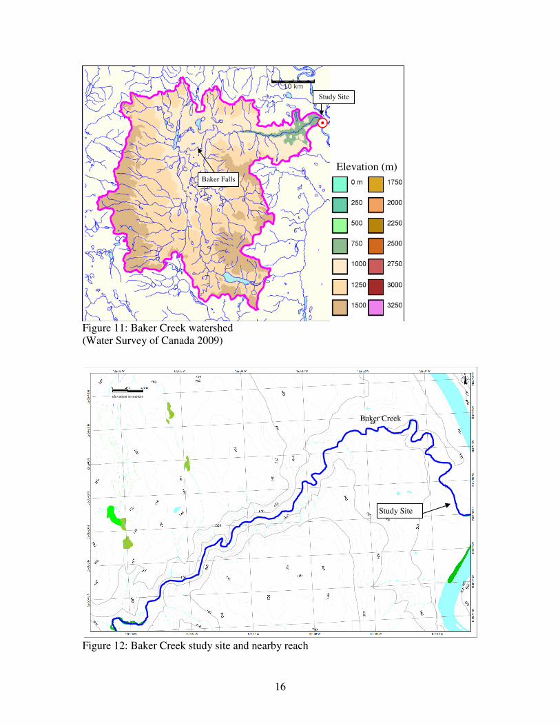
The 1570 km2 watershed of Baker Creek (WSC# 08KE016, 52°58” N, 122°31” W), is

located in the interior plateau of BC and has a nival flow regime with a maximum and

mean discharges of 129 m3/s and 5 m3/s, respectively. Watershed elevations range from

15

480 m to 1520 m (Figure 11). Young forest, clearcuts (~40%), agriculture and wetlands

are the primary land uses in the watershed with Sub-Boreal Pine – Spruce,Sub-Boreal

Spruce and Montane Spruce dominate the forest. Gravel sized sediment is provided by

glaciofluvial colluvium along a deeply incised, meandering canyon that ends 2 km

upstream of the field site.

Figure 10: Baker Creek photo looking upstream from bridge

16

Elevation (m) Baker Falls

Study Site

Figure 11: Baker Creek watershed (Water Survey of Canada 2009)

elevation in meters

Study Site

Baker Creek

Figure 12: Baker Creek study site and nearby reach

17

The 206 m long study reach starts about 50 m downstream of the gauge (see Figure 13).

A bridge narrows the creek downstream of the study reach with ongoing sediment

deposition on the upstream side of the bridge causing a steep bed gradient and

supercritical flow under the bridge. Therefore, the bridge acts as a flow control for the

gauge and the flow was set to critical depth at the downstream end of the model. The

channel thalweg crosses the channel from right to left bank and is paved with angular

boulders. The right bank has riprap at the upstream end transitioning to cohesive

sediments with roots at mid reach, and to gravel and silt at the downstream end, whereas

the left bank consist of gravel filled in with silt and sand.

N

H

40m

G = WSC Gauge H = WSC Manual Measurement Location Contour Interval 0.36m Elevation Relative to WSC datum

Flow

Bridge

G

Figure 13: Baker Creek modeled reach

Finally, East Creek is located in the UBC Malcolm Knapp Research Forrest (49°16” N,

122°34” W), and is used for ongoing monitoring of sediment transport and channel

morphology of a small mountain stream (Oldmeadow and Church, 2006; Caulkins and

Hassan, 2007; and Hassan et al., 2009). The bed topography along ~300m of the study

reach has been regularly surveyed every year since 2003, bedload traps and gravel tracers

are used to measure sediment transport. The creek has a mobile bed, a 1.17 km2

catchment, and mean annual and maximum discharges of 0.09 m3/s and 2.6 m3/s,

18

respectively. The region has a maritime climate with wet mild winters and warm dry

summers and the entire watershed is a Coastal Western Hemlock biogeoclimatic zone.

Streamflow responds rapidly to rainfall and periods of low flow dominate during the

summer months (Scordo and Moore 2009).

The upper portion of the creek is relatively steep, dominated by step-pool morphology.

The gradient then flattens across a sediment wedge immediately upstream from a culvert

through which the passage of cobbles is restricted (Oldmeadow and Church, 2006). Sand

and gravel pass through the culvert and are measured using two sediment traps before

being returned to the creek (Caulkins and Hassan, 2007). Immediately downstream from

the culvert is a deep plunge pool followed by a long channelized section with average

gradient of 0.020 and a rapids then riffle-pool morphology. The upper most part of the

monitored reach, upstream of the modelled reach, is narrow and the channel is incised

into old glacial till with large material. The till is the source of cobbles and boulder sized

sediment and the study was carried out along 290 m meters of the riffle-pool portion of

this reach (Figure 15).

19

Figure 14: East Creek photo looking downstream. (Photo by J. Caulkins)

N

Contour Interval 0.4m Elevation relative to MASL

15m

Flow

Figure 15: East Creek modeled reach

20

Study Reach

Figure 16: East Creek watershed

21

4 METHOD The method can be separated into the numerical and field components and is presented in Figure 17.

Figure 17: Method flow chart (Blue boxes are initial inputs)

4.1 Numerical Model

In shear stress equations the flow depth, flow area and wetted perimeter variables are

often not clearly defined (Smart, 2001) because they are typically calculated from

channel surveys and are not related to bed roughness. Our topographic survey has spacing

Estimate

Water Level

Grain-size Survey & Fit to

Log-normal Distribution

Refined Total-station

Survey

Structured Grid

Cross-sectional area of topographic survey

Wetted Perimeter

Protruding cross-sectional area of roughness elements perpendicular to the approach velocity

Cross-sectional area of water

Hydraulic Radius

Friction Slope

Wiberg and Smith Velocity Profile

Boussinesq Coefficient Discharge

Vegetation Survey

St. Venant Momentum

Balance

Iterate

22

1-2 orders of magnitude larger than the D50 grain size that forms the bed and therefore the

three geometric parameters need to relate to both the macro-scale topographic survey and

the micro-scale roughness survey. This is particularly necessary for spatially-variable

roughness, where the vertical velocity profile is calculated locally and is more sensitive to

macro-scale averaging of these parameters.

Kean and Smith used standard calculations of the wetted perimeter (Ptopo) and cross-

sectional area of flow (Atopo) based on the topographic survey. For this study three new

formulae were derived to calculate cross-sectional area of water (Aflow), depth of flow

(hflow), and wetted perimeter (Pflow) that are based on the local sediment distribution

derived from the roughness survey (Figure 17), and the hydraulic radius was calculated

from Pflow and Aflow. See Appendix A for the derivations.

Figure 18: Visual depiction of the geometric parameters used in the study

Calculating the exact wetted perimeter depends on measurement resolution (Mandelbrot,

1967) which is limited by the steps between the size classes of the Wolman (1954) pebble

count. The model uses a structured grid and each cross-section is divided into subsections

(i) of roughly equal width (Bi). Assuming no stacked grains (Wiberg and Smith, 1991),

the Pflow for each subsection (Pi) was calculated using equation (7).

( ) ( )

( )

−−

−+= ∑∑

∑ >==

=

+M

hwhereDm

mitopoimz

M

m

mimzM

m

mimz

itopoitopoi

i

iz

chDcDs

cD

hhBP ,,,

0

,,1

0

,,

2

1,,

2

2

(7)

The probability (cm) is a discrete version of the log-normal distribution (Wiberg and

Smith, 1991) for the individual grain-size classes (Dz,m) and s1 is a shape factor. The

grains were assumed to have a parabolic shape (Smart et al., 2004), therefore s1=2.96. As

23

the roughness parameters were mapped, the topographic surveyed depth (htopo) was

calculated as the distance from the water surface to the topographic survey elevation, and

the total Pflow was determined for each cross-section as

=∑

i

iflow PP . Equation (7) also

assumes that the centres of the representative grain-sizes (Dm) are in a line along the

cross-section and while this is false, and could result in a positive bias in the wetted

perimeter, it is believed to be offset by the assumption that the grains are not stacked.

The Wiberg and Smith (1991) assumption of no flow blockage by grain particles is

“potentially the most important effect that is neglected by the model” (Carney et al.,

2006). For high relative roughness conditions a traditional survey could not accurately

portray the flow pattern between boulders. To better represent the impact of large

roughness elements on the flow, the field survey mapped only the low points between the

boulders (Figure 18) and the expected protruding cross-sectional area of the bed

roughness perpendicular to the approach velocity ( )grainsA was calculated and added

above the survey plane. This in turn restricted the cross-sectional area of water (Aflow)

and helps accounts for flow blockage. grainsA was determined from equation (8) and

subtracted from the cross-sectional area of the topographic survey (Atopo) to calculate

Aflow in equation (9).

i

iDigrains

AA

θ

,, = (8)

∑ −=i

igrainsitopoflow AAA ,, (9)

θi is the proportion of the subsection width (Bi) taken up by the width of one average

grain, which is similar to the blocking ratio described by Smart et al (2004). iDA , is the

cross-sectional area perpendicular to the approach velocity of an average single grain. An

estimate of the submerged boulder area, for each subsection of the cross-section, was

calculated using equation (10).

24

( )

−−= ∑∑

∑ >=≤=

=

M

hwhereDm

mtopomztopo

M

hwhereDm

mmzM

m

mmz

iigrains chDhcD

cD

BA

m

2

,

222

,

0

,

, 2

4

π (10)

The flow depth can be derived as a function of the cross-sectional area of water (equation

(12)).

.

∫= dyhA flowflow (11)

( )

−−−= ∑∑

∑ >=≤=

=

M

hwhereDm

imitopoimzitopo

M

hwhereDm

imimzM

m

imimz

itopoiflow chDhcD

cD

hhm

2

,,,,

2

,

2

,

2

,,

0

,,,

,, 2

4

π (12)

To restrict the model results to gradually varying flow the critical depth was calculated

and used as the lower boundary of the stage solution. Since each cross-section in the

structured grid is discretized into multiple subsections with multiple depths and

discontinuities in area. Numerically this leads to more than one local minimum in the

specific energy of flow and hence more then one numerically calculated critical depth

(Traver, 1994, and Chaudhry, 2008). To achieve a single ‘critical depth’ for a cross-

section Traver (1994) calculated depth-average velocities for each subsection (i) of the

cross section using Manning’s n. Alternatively, Kean and Smith (2005) calculated an

average critical Froude number (Fr) for the entire cross section by solving equation (13)

for the critical water surface elevation (WScritical) using the bed elevation for each

subsection (zi).

( )1=

−

==

∑ topo

i

iicriticaltopotopo gRBzWS

Q

gRA

QFr (13)

However, an average Froude number does not account for the spatial variability of the

flow across the channel and effectively interpolates the non-linear cross-section as a box

culvert with area and height of Atopo and Rtopo respectively. In this study, the critical depth

25

was determined by assuming that Fr is critical at all points in the cross-section,

preserving much of the cross-sectional shape, and the water surface elevation was

calculated using equation (14).

( )1

23=

−=

∑i

iicritical gBzWS

QFr (14)

The St. Venant equations were solved for the water slope by specifying the downstream

stage to the critical depth. Alternatively Kean and Smith (2005) specified the water slope

and solved the equations for the stage. The modeled stream reaches included the

‘control’, where the model typically calculated critical depth, and hence, the downstream

stage provided negligible influence on the modeled stage height. If there had been

backwater conditions then the critical depth assumption would not have been fulfilled and

a two-stage model (Schmidt and Yen, 2008) or a variable slope model (Kean and Smith,

2005) would need to be used.

The numerical model was solved using the Newton-Rhapson iteration technique

(Pappenberger et al., 2005) in a simultaneous solution procedure (Chaudhry, 2008). The

program was coded in FORTRAN and the derivatives were discretized using a second

order Taylor series approximation. Multiple channels were accommodated through the

use of subsections. Each cross-section was divided into discrete subsections containing

roughness parameters and a bed elevation unique to that subsection. The velocity profile

was calculated and integrated for each subsection, and the individual values for the

subsection discharge, area and wetted perimeter were summed for the entire cross-

section. This provides a single node of information for each cross-section within the 1D

model and multiple channels retained their own flow depths as well as Boussinesq and

Chezy coefficients.

The Wiber and Smith (1991) velocity profile algorithm required iteration to derive the

flow field )/( *uu at any point in the water column, and the flow field was integrated

26

over the depth and used in equation (5) to calculate the Chezy coefficient. When applied

in a spatially-variable manner, this method involves a dozen iterations at thousands of

locations for each step in the Newton-Rhapson procedure and hence the numerical

approach is not computationally efficient, which is likely why it has not been widely

used.

4.2 Field Surveys

Since the resolution of the stream-bed topography controls the performance of the

numerical models (Pappenberger et al., 2005; and Hardy, 2008), separate surveys were

conducted to measure the channel shape and the bed surface texture. Channel shape and

surface texture surveys have typically involved simple mapping of the bed using a total-

station and a single spatially averaged measurement of the roughness. However, this

introduces elevation uncertainty at the same scale as the roughness elements, which can

be significant for large roughness, and can be exacerbated by spatially-variable roughness

elements.

To improve the channel survey resolution, a theodolite-based total station was used and

only the local minimum elevations between the bed particles were measured. This

enabled the direct estimation of the roughness and its superimposition on the mapped bed

(Figure 18). Such a method resolves the Wiberg and Smith (1991) assumption that the

bases of the bed particles all rest on a collective plane by establishing a realistic datum

for the sediment. The survey spacing averaged one survey point per 1.2 m2 for Alouette,

per 2.25 m2 for Cayoosh and Baker, and per 0.25 m2 for East Creek.

Bed surface texture was determined using the Wolman pebble count (Wolman 1954).

Where the bed was dry photographs were also taken of the sediment and analyzed using

‘gravel-o-meter’ software. For large scale roughness, such as boulders and steps, a

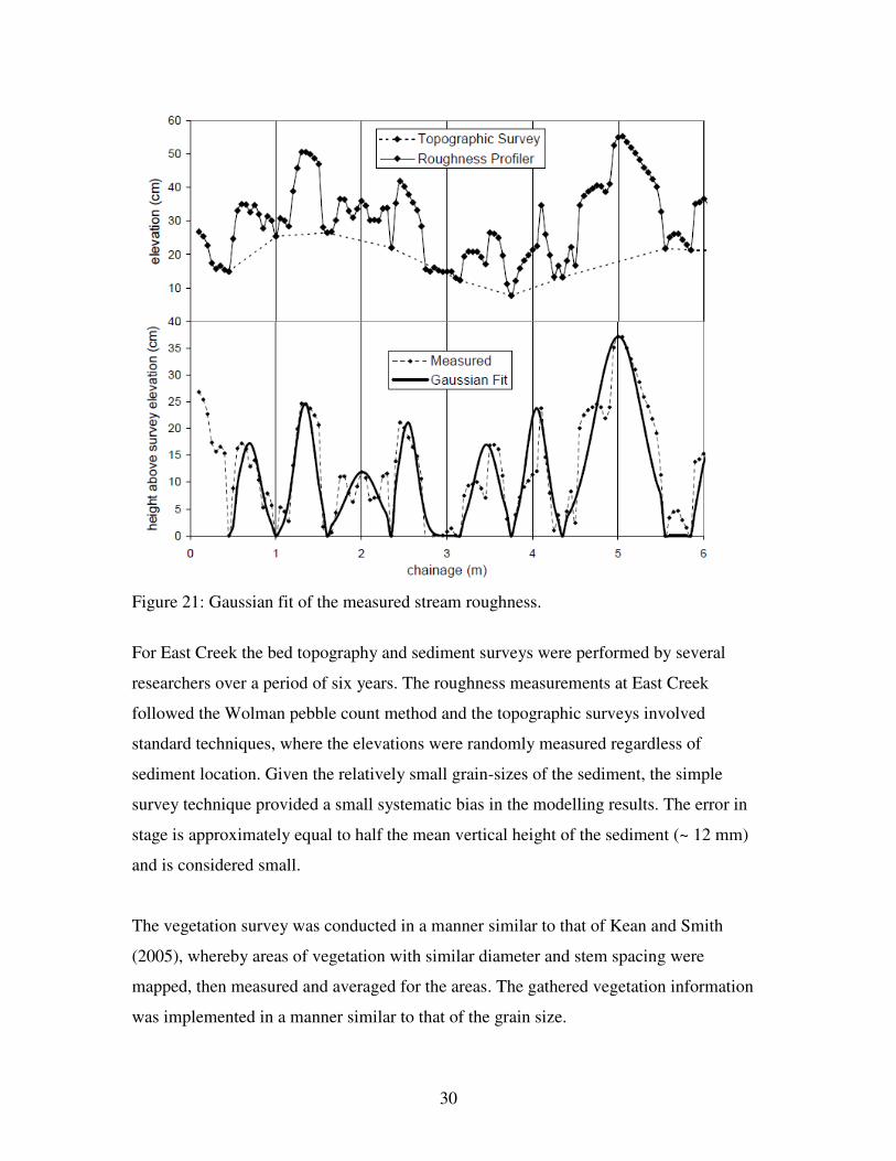
bedform profiler (de Jong, 1995, and Smart et al., 2004), was used with 5 cm rod spacing.

The profiler elevations were adjusted to remove the channel shape, and separated into

individual roughness elements. The maximum, mean and standard deviation were

calculated from the heights of these pieces as shown in Figure 21. The profiler measured

27

the vertical axis (Dz) and the Wolman pebble count measured the intermediate axis (Dx).

Following Wiberg and Smith (1991) it was assumed that

zx DD 2= (15)

Where the water was too deep for a Wolman pebble count, the photo software, or the bed

profiler, the maximum diameter was measured, the mean was estimated and the standard

deviation was calculated as one third of the distance from the estimated mean bed level to

the tops of the largest boulders (Smart, 2001). For large roughness, a second topographic

survey was completed that measured the elevation of the tops of the boulders and was

compared against the main topographic survey to provide a check on the estimate for the

maximum vertical diameters.

The vast majority of numerical models have assumed that bed particles are randomly

distributed throughout the reach. This supports the use of a single, spatially-averaged

roughness parameter, which simplifies the grain-size surveys and enables reach-scale

flow resistance equations. Moreover, spatially averaged stream roughness can be

calibrated from velocity measurements and the use of a resistance equation. However,

simple spatial averaging trivializes the non-linear relationship between flow and

roughness, and there have been limited attempts to incorporate spatially-distributed

channel roughness into flow models (Aronica et al, 1998, Folk and Prestegaard, 2000,

and Lisle et al., 2000).

An alternative to simple spatial averaging is to assume that local flow responds to local

grain size requiring a spatial representation of the roughness throughout the reach.

Therefore, morphologically similar areas (i.e., similar roughness) were surveyed, and

mapped to the same structured grid used for the topography of the channel. This implies

that every point in the topography grid included a corresponding maximum, mean, and

standard deviation of the roughness height (Figure 19). This method requires more

detailed survey notes, but necessitates only a marginal increase in survey time. Such

spatial mapping also resolves the assumption of spatially-averaged roughness in the

Wiberg and Smith (1991) model.

28

Figure 19: Sample of spatially-variable roughness data for the modeled reach of Cayoosh Creek.

To further exemplify the differences between the spatially-averaged and spatially-

variable methods, the spatially averaged values of the maximum, mean, and standard

deviation of bed surface texture are presented in Table 1. The flow model was re-run for

the sites using these single spatially-averaged statistics (see results). For comparison and

in order to illustrate the differences between the methods, the spatially-averaged grain-

size distribution and the range of obtained distributions are presented in Figure 20.

Table 1: Spatially-averaged grain-size statistics.

Alouette

River

Cayoosh

Creek

Baker

Creek

East

Creek

Max Diameter (Dx,max)

696 mm 980mm 500 mm 512 mm

Phi Mean ( xφ ) -5.53 (46 mm)

-5.59 (48 mm)

-5.22 (37 mm)

-5.34 (41 mm)

Phi Standard

Deviation (xφσ ) 1.92 1.51 1.33 1.13

Notes: ( ( )xD2ln−=φ )

xφ was calculated as the arithmetic mean of the local phi-means.

xφσ was calculated as the root-mean-square of the local phi-standard deviations.

29

Figure 20: Comparison between the spatially-averaged and

spatially-variable grain-size distributions.

30

Figure 21: Gaussian fit of the measured stream roughness.

For East Creek the bed topography and sediment surveys were performed by several

researchers over a period of six years. The roughness measurements at East Creek

followed the Wolman pebble count method and the topographic surveys involved

standard techniques, where the elevations were randomly measured regardless of

sediment location. Given the relatively small grain-sizes of the sediment, the simple

survey technique provided a small systematic bias in the modelling results. The error in

stage is approximately equal to half the mean vertical height of the sediment (~ 12 mm)

and is considered small.

The vegetation survey was conducted in a manner similar to that of Kean and Smith

(2005), whereby areas of vegetation with similar diameter and stem spacing were

mapped, then measured and averaged for the areas. The gathered vegetation information

was implemented in a manner similar to that of the grain size.

31

5 MODEL RESULTS AND DISCUSSION The modelled stage-discharge relations are compared against manually measured stages

for specific discharges in Figure 22 through Figure 25, with uncertainty calculated as

described by Herschy (1999), and the results are discussed in reference to the main

assumptions. The Water Survey of Canada (WSC) measured the manual discharges for

Alouette River, Cayoosh Creek and Baker Creek between 2007 and 2009 using the

velocity-area method (Herschy 2008). The locations of the WSC measurements, and

where the results were extracted, is depicted by the H in Figure 5, Figure 9, and Figure

13.

The sites are presented in the order of their channel bed modelling complexity. Alouette

has simple small-scale roughness, Cayoosh has large-scale roughness, Baker has a mobile

bed, and East Creek has a mobile bed that is modelled over a period of years. The model

for East Creek was run for each of the six survey years and, to highlight the effects of bed

mobility (scour and fill) on the stage-discharge relation, curves for each survey year are

presented for five cross-sections along the study reach. None of the model parameters

were calibrated.

5.1 Alouette River

The modelled and measured discharges for Alouette River are presented in Figure 22.

Lisle et al (2000) and Wiberg and Smith (1991) assumed the bed particles could be

spatially-averaged, leading to a spatially-constant drag coefficient. Implicit in this

assumption is that either the bed particles are randomly distributed or that the flow is not

affected by positioning of roughness over the reach. Such spatially-averaged roughness

may be adequate for relatively homogeneous bed morphology (Kean and Smith, 2005)

but it consistently underestimated the stage at Alouette River (see Figure 22). Near bed

shear stress and the vertical velocity profile adjust to changes in roughness in a complex

and non-linear manner (Lisle et al., 2000, and Yen, 1999). A simple averaging of the

roughness could obscure the non-linear force balance in the water column and bias the

momentum balance.

32

In the Alouette reach, the finer sediment is located on the banks of the river and larger

sediment located in the thalweg. When the grain-sizes were spatially-averaged, the mean

sediment diameter was suppressed for the thalweg region, where the highest velocities

are located, and the maximum sediment diameter was over estimated on the edges of

each cross-section. This resulted in higher momentum in the deep central portion of the

flow, lower momentum in the shallow outer portions of the flow, and overall a higher

total momentum. Overestimating the momentum reduces the cross-sectional area of water

needed to convey the flow and hence underestimates the stage.

Figure 22: Alouette River model verification using measured data from

Errors in the survey measurements are considered small and random compared to the

systematic functional error. Functional errors are a result of the reduction of the complex

physics inherent in turbulent open channel flow into a discrete, one-dimensional set of

equations with a detached and simplified roughness model. Freeman et al (1996)

determined that the single most important source of error in stage-discharge modelling is

within the roughness coefficient. Kean and Smith (2005) calibrated their roughness

33

length to stage-discharge measurements, which likely helped to reduce the roughness

error, while the roughness length was calculated from the grain size statistics for this

study. Bohorquez and Darby (2008) varied the roughness length of a 1D momentum

model to estimate the model error, and a Monte Carlo model (Pappenberger et al. 2004)

could be used to assess the sensitivity of the roughness length on the model.

Because we used a 1D momentum model, additional functional error can arise when

trying to model flows that incorporate significant two- and three-dimensional effects (e.g.

secondary circulation, dispersion, and turbulence - Hardy, 2008). Two-dimensional

stream models (Wilson et al., 2002) could alleviate much of the functional error and

three-dimensional models (Jazizadeh and Zarrati, 2008) have the same number of

dimensions as the underlying processes. Unfortunately this results in an increase in

measurement error as additional dimensions require unrealistically fine spatial detail to

define the roughness surface (Horritt and Bates, 2002), or to support additional roughness

parameters (Hardy, 2008, and references therein). However, it would be worthwhile to

evaluate the spatially-distributed roughness and new formulae for flow area and wetted

perimeter within two and three-dimensional momentum models.

With the 1D model a sensitivity analysis should be done to determine the maximum

survey spacing, as well as the corresponding structured grid spacing, needed for an

accurate model, as there is a point where accuracy gained through additional survey

measurements is negated by the functional error. It may be possible to reduce the number

of grain-size measurements down to a handful of surveys, each of which runs along an

estimated flow streamline, although streamwise sorting (Lisle and Madej, 1992) may

negate any benefits.

5.2 Cayoosh Creek

For Cayoosh Creek, the modeled stage-discharge relation was calculated using three

methods: 1) with spatially-variable roughness and using the Wiberg and Smith (1991)

model for the velocity profile, 2) with spatially-averaged roughness and the Wiberg and

Smith (1991) model, and 3) with spatially-variable roughness and the simple log-law

34

model. All three models underestimate the stage for low flows by 0.2 m, while method 3

also underestimates the stage at medium flows (20-40 m3/s) leaving the Wiberg and

Smith model as the best estimate for stage at these flows. The mean annual flood for

Cayoosh is 96 m3/s but the WSC does not have any recent measurements higher then

what is shown in Figure 23.

Figure 23: Cayoosh Creek model verification using measured data from The low flow discrepancy is not believed to be the result of incorrect model datum, or

bed movement prior to the survey. The low flows are controlled by a natural weir-like

crest at the downstream end of the gauge-pool that had formed a riffle (see Figure 24).

The bed material at the pool-crest is primarily boulders and sand and the funnelling of the

water through the riffle, due to sediment imbrication, may have increased the upstream

stage. The spatially-averaged distribution model consistently underestimated the stage at

Cayoosh Creek, which is similar to the Alouette results although the difference is not as

dramatic. The small difference is possibly due to the more spatially uniform grain size

distribution at Cayoosh and the thalweg is not as pronounced as at Alouette.

35

Figure 24: Close-up of riffle at downstream end of the gauge-pool at Cayoosh Creek.

The large roughness model (Wiberg and Smith, 1991) significantly influenced both the

Chezy and Boussinesq coefficients within the momentum calculations. The modifications

to the Kean and Smith (2005) method helped address the Wiberg and Smith assumptions

regarding flow blockage by sediment, grains not being stacked, and spatially-averaged

roughness. Neglecting the shadowing effects of sediment in the streamwise direction may

have the most impact on the current model since the cross-sectional area of water and

wetted perimeter calculations only addresses the sediment geometry in the transverse

direction. Additional roughness survey techniques such as sand spreading, laser scanning,

low level aerial photography and line-by-number sampling have been used to estimate

sediment imbrication (Smart el al., 2002, and Smart et al., 2004). Unfortunately most of

these methods require a dry bed except line-by-number sampling, which may be

complimentary to the methods used in this study. If the shadowing effect is quantified, it

is uncertain how this could be incorporated into the Wiberg and Smith model.

Alternatively sediment imbrication could be represented by a hiding functions (Parker,

1990), but combining it into the velocity profile model would also require further

research.

Grain-size measurements at Cayoosh involved a combination of direct measurement of

the vertical axis diameter and indirect calculation of the vertical axis from intermediate

axis measurements. The Wiberg and Smith model assumes that 2Dz=Db-axis and is

supported by Green (2005). Comparisons were made between the vertical and

intermediate axes of the grains and although the relation between the two could be

roughly 2:1, there is a wide variation. This assumption could be resolved by measurement

of only the vertical axis in the field, which eliminates the photo analysis technique but

36

line-by-number sampling (Smart el al., 2002) could be used to provide an additional

check. Also it may not be necessary to do full grain-size distribution analysis, when

perhaps the distribution of the 10 largest grains, or the hybrid technique (Rice and

Haschenburger, 2004), or the topsum technique (Clancy and Prestegaard, 2006) could

formulate an accurate velocity distribution utilizing the Wiberg and Smith (1991)

approach, and reduce the time spent surveying.

5.3 Baker Creek

Baker Creek is unstable relative to Alouette River and Cayoosh Creek. The stage-

discharge relation for the gauging station at Baker Creek is dominated by the channel

shape at the downstream bridge. This provides a critical flow control at all discharge

levels, and therefore the choice of roughness distribution, spatially-averaged or spatially-

variable, had no influence on the model results (Figure 25). The flood frequencies in

Figure 25 were calculated assuming a Gumbel distribution. The model results are in good

agreement with measured discharges for the 2008/09 water year, the same year that the

survey was completed (Figure 22). However, there is a significant difference between the

modeled and the measured stages for years prior to 2008. The manual measurements for

Alouette River and Cayoosh Creek were below the mean annual flood, and hence the

flood frequencies were off the chart in Figure 22 and Figure 23.

37

Figure 25: Baker Creek model verification using measured data The measured values align closely with the calculated values for the year of the physical survey (June 2008 – April 2009). Significant bed movement occurred during the freshet in May 2008 and the model does not align with the values that were manually measured prior to 2008.

In May of 2008 the gauge site experienced a 50 year flood, which may have significantly

altered the bed topography and stage-discharge relation. Piecewise linear stage-discharge

relations before and after the flood suggest a shift from 6.8 m3/s to 2.5 m3/s for the 1.42

m stage (Figure 22). The two curves are roughly parallel when plotted in log space

therefore the difference in discharge increases as the stage increases, resulting in a shift

from 76 m3/s to 48 m3/s at the 2.58 m stage. This upward shift in the stage-discharge

curve suggests there was a net sediment deposition at the gauge location and, as noted by

Kean and Smith (2005), this type of model is not designed for unstable channels.

Baker Creek reinforces the fact that stage-discharge relations are dynamic (Dottori et al.,

2009). Water resource managers often make decisions based on real-time discharge data,

but adjustments to the relations, due to geomorphic change, continue to lag stage

measurements by months and the changes are normally applied retroactively (Hamiton,

38

2009). There is a growing call for improved modelling to enable real-time adjustments of

stage-discharge relations (DeGagne, 1996, Cao and Carling, 2002, Kean and Smith,

2005, Hardy, 2008, Dottori et al., 2009, and Juracek and Fitzpatrick, 2009), and the

results from Baker and East Creeks contribute to this call.

5.4 East Creek

Following the Baker model, East Creek was subsequently modeled to demonstrate how

the stage can shift in a mobile bed. The numerical model for East Creek calculated stages

along the reach for six separate topography surveys taken over six years (2003 to 2008).

The resulting stage-discharge relations for several specific cross sections are presented in

Figure 26 and the corresponding cross-sections are presented in Figure 27. The pin

numbers indicate the nearest established survey markers.

Figure 26-Pin#38 shows a location where the stage-discharge curve changed very little,

possibly due to no change in the topography (see Figure 27). It demonstrates how a well-

selected site could have very little change in the stage-discharge relation over time.

Figure 26-Pin #40 & #41 demonstrate the large changes in theoretical stage-discharge

curves that occurred between years, with the most dramatic changes occurring in the

winter of 2006/2007. Between 2004 and 2005 the discharge at pin #140 shifted from 1.2

m3/s to 2.0 ms/s for the same stage (134.60m). This was followed by shifts down to 1.55

m3/s then up to 2.2 m3/s at the same stage for 2006 and 2007, respectively.

The results for pin #146 were more dramatic, where the discharge went from 2.9 m3/s to

0.9 ms/s then to 0.4 m3/s for the same stage (133.30m) over the years 2006, 2007 and

2008, respectively. Correlating this to flood peaks, East Creek experienced one bankfull

event during the winters of ’03/’04 and ’04/’05, zero events in ’05/’06, and three bankfull

events during the winter ’06/’07 (Caulkins, 2009). The corresponding cross-sections in

Figure 27 do not show a large change between years as the bed shift changes occurred

downstream of both locations. However there was significant bed shifts downstream of

both sittes (Figure 28).

39

Figure 26-Pin #47 & #52 show modelled results for locations where there were large

shifts in the upper or lower portions of the stage-discharge curve respectively, with small

changes in the curves at the opposite ends. In Figure 26-Pin #52 the lower part of the

stage-discharge curve could have shifted as a result of erosion (or fill) of the low water

control, while the mid-stage and high-stage part of the bed may have retained the original

shape. Hence at high water the high stages maintained the previous stage-discharge

relationship when the influence of deposits (or erosion) on low-water control were

drowned out. Thus the scour and fill of the low water control resulted in a series of stage-

discharges that spread out fanwise at the low flows. The opposite may also occur where

the low water control is stationary, due to armouring or bedrock, and there is deposition

or erosion at the high levels during floods causing an opposite fan of curves (see Pin

#47). The corresponding cross-sections in Figure 27 displays bed shifts on the banks and

in the thalweg for Pin #47 and #52 respectively.

Figure 25 and Figure 26 illustrate how various different types of shifts in the stage-

discharge relation may be necessary depending on the nature of the gauging location and

bed movement. Following a channel mobilizing event conventional stream gauging

requires a manual measurement of stage (hmanual) and discharge (Qmanual) to determine the

bias (∆h) in the old stage-discharge relation at Qmanual. Then one or more portions of the

stage-discharge relation are adjusted. The adjustment is primarily a shift in the relation at

Qmanual, where the shift may be equal to or less than ∆h. There are also secondary shifts in

the relation for discharges that are higher and lower then Qmanual, but those secondary

shifts may be equal to ∆h at all discharges, or may be weighted by previous manual

measurements, or may be weighted by the magnitude of the discharge along the curve.

This leads to many different ways in which a relation can be adjusted, the effectiveness of

which depends on the skill and intuition of the hydrographer (DeGagne et al., 1996).

40

Figure 26: East Creek modeled stage-discharge at various pins for multiple years

41

Figure 27: East Creek surveyed bed shape at various pins for multiple years

42

Figure 28: East Creek surveyed bed shape immediately downstream of the modelled locations for Pin #40 and #41

43

6 CONCLUSION

A one-dimensional model of momentum balance incorporated two roughness models to

calculate theoretical stage-discharge relations at four sites in British Columbia that range

in bed stability, bed structure, hydrology and sediment supply. To better account for the

non-linear relationship between flow and the spatially-variable grain-size distribution,

spatially-distributed roughness was incorporated into the Kean and Smith (2005) model.

The standard topographic field survey was adjusted to include simple, specific

measurements. This was combined with three new formulae for geometric parameters

that reduce the overall uncertainty in the topographic input and eliminate assumptions

from the roughness model.

The results show how (1) spatially-distributed roughness yielded better results than

spatially-averaged roughness, (2) the stage-discharge relation shifted in response to a

flood (Baker), and in response to annual bed movement (East Creek), and therefore, (3)

the relations must be re-evaluated following events that mobilize the bed. For the two

relatively stable reaches (Alouette and Cayoosh), (4) the modelled results were similar to

those measured by the Water Survey of Canada and the method can be used to estimate

high flows and flows in remote, stable locations.

Until new technology allows stream discharge to be measured directly, stage-discharge

relations will remain a necessity. Accurate numerical modelling is crucial to define stage-

discharge relations for new sites. For existing gauges the modelling can update the

relations following any bed movement, which is particularly useful for the numerous

unstable mountain-streams in BC. To ensure the numerical model is independent of the

empirical approach of generating stage-discharge relations, the model cannot be

calibrated to the same manual measurement used for the empirical approach. The

empirical method is not practical for unstable beds, as the manual measurements are

taken over a period of months or even years, in which time the beds shift. Numerical

modelling provides an immediate stage-discharge relation from a single site survey. This

44

is useful when hydrometric sites are created or moved, and as survey tools improve so do

the speed and cost of surveys.

The model used in this study required no calibration, reducing the equifinality of

parameters (Aronica et al., 1998, and Pappenberger et al., 2004) and provides an

independent check on standard empirical methods. However, the level of validation was a

coarse comparison between the model and measured stages for a given discharge. The

validation could become more specific with more data, such as localized shear stress,

sediment movement, and velocity profiles. This method can compliment the popular

empirical approaches to developing stage-discharge relations, but to provide a realistic

alternative to the popular approaches this model needs to be further validated for various

bed types at high discharges.

45

7 REFERENCES

Aronica, G., B. Hankin, K. Beven (1998), Uncertainty and equifinality in calibrating distributed roughness coefficients in a flood propagation model with limited data, Advances in Water Resources, 22(4). Baldassarre G. Di., A. Montanari (2009), Uncertainty in river discharge observations: a quantitative analysis, Hydrology and Earth System Sciences, 13, pp. 913–921. Bhattacharya, B., D.P. Solomatine (2005), Neural networks and M5 model trees in modelling water level-discharge relationships, Neurocomputing, 63, pp. 381-396. Bohorquez, P., and S.E. Darby (2008), The use of one- and two-dimensional hydraulic modeling to reconstruct a glacial outburst flood in a steep Alpine valley, Journal of Hydrology, 361(3). Braca, G. (2008), Stage-discharge relationships in open channels: Practices and problems, FORALPS technical reports, 11. Università degli Studi di Trento, Dipartimento di Ingegneria Civile eAmbientale, Trento, Italy, 28, pp. 24. British Columbia Conservation Foundation (1999), Alouette River Gravel Replacement, Prepared for BC Hydro Bridge Coastal Restoration Program, 99-LM-09. British Columbia Conservation Foundation (2005), Habitat Assessments and Restoration Prescriptions for the Corrections Reach of the Alouette River, Prepared for BC Hydro Bridge Coastal Restoration Program, 05-AL-01. British Columbia Conservation Foundation (2006), South Alouette River Fish Habitat Restoration Project, Prepared for BC Hydro Bridge Coastal Restoration Program, 06-ALU-03. Cao, Z., P. A. Carling (2002), Mathematical modelling of alluvial rovers: reality and myth. Part 1: General review, Proceedings of the Institution of Civil Engineers, Water and Maritime Engineering, 154(3). Carney, S. K., B.P. Bledsoe, and D. Gessler (2006), Representing the bed roughness of coarse-grained streams in computational fluid dynamics. Earth Surface Processes and Landforms, 31, pp. 736–749. Caulkins, J.L., 2010. Sediment transport and channel morphology within a small, forested stream: East Creek, British Columbia. Unpublished dissertation, University of British Columbia, Vancouver. Caulkins, J., M.A. Hassan (2007), Spatial and Temporal Patterns of Sediment Transport in a Small Stream, Eos Trans. AGU, 88(52), Fall Meet. Supplemental.

46

Chaudhry, M.H. (2008), Open Channel Flow, 2nd ed., pp. 151-197, Springer. Chen, Y.C. and C.L. Chiu (2004), A fast method of flood discharge estimation, Hydrological Processes, 18, pp. 1671-1684. Chow V. T. (1959), Open Channel Hydraulics, McGraw-Hill, New York. Clancy, K. F., and K. L. Prestegaard (2006), Quantifying particle organization in boulder bed streams, in 4th Iahr Symposium on River, Coastal and Estuarine Morphodynamics, ed. G. Parker, and M.H. Garcia, Published by Taylor & Francis. de Jong, C. (1995), Temporal and spatial interactions between river bed roughness, geometry, bedload transport and flow hydraulics in mountain streams—Examples from Squaw Creek (Montana, USA) and Lainbach/Schmiedlaine (upper Bavaria, Germany), Berlin. Geogr. Abh., 59, pp. 1–229. DeGagne, M.P.J., G.G. Douglas, H.R. Hudson, S.P. Simonovic, (1996), A decision support system for the analysis and use of stage–discharge rating curves, Journal of Hydrology 184, pp. 225– 241. Does, T., G. Morgenschweis, and T. Schlurmann (2002), Extrapolating stage-discharge relationships by numerical modeling, In: Proceedings 5th International Conference on Hydro-Science and Engineering (ICHE-2002), September 18–21, Warsaw, Poland. Dottori, F., M. L. V. Martina, and E. Todini (2009), A dynamic rating curve approach to indirect discharge measurement, Hydrology and Earth System Sciences, 6, pp. 859–896. Fischenich, C. and S. Dudley (2000). Determining drag coefficients and area for vegetation, EMRRP Technical Notes Collection, TN EMRRP-SR-8, U.S. Army Engineer Research and Development Center, Vicksburg, MS. Folk, K. A., K. L. Prestegaard (2000), The Organization of Boulders and Associated Velocity Fields in Natural Streams, Eos Trans. AGU, 81 (48), Fall Meet. Suppl., Abstract NG71B-24.

Freeman, G.E., R.R. Copeland, and M.A. Cowan (1996), Uncertainty in Stage Discharge Relationships, in: Stochastic Hydraulics, Proceedings of the 7th Symposium on Stochastic Hydraulics, IAHR, pp. 601-608.

Freeman, G.E., W.H. Rahmeyer, and R.R. Copeland (2000), Determination of resistance due to shrubs and woody vegetation, Technical Report, ERDC/CHL TR-00-25, U.S. Army Engineer Research and Development Center, Vicksburg, MS.

47

Gawne D. K. and S. P. Simonovic, (1994), A computer-based system for modelling stage-discharge relationship in steady-state conditions. Journal of Hydrological Sciences, 39(5), pp. 487–506. Green, J.C. (2005), Choice of Percentiles and Axes to Determine Grain Resistance, Journal of Hydraulic Engineering, 131(11). Hamilton, S. (2009) Personal Communication. Hardy, R.J. (2008), Geomorphology Fluid Flow Modelling: Can Fluvial Flow Only Be Modelled Using a Three-Dimensional Approach?, Geography Compass 2(1). Hassan, M.A., M. Church, J. Rempel, and R.J. Enkin (2009), Promise, performance and current limitations of a magnetic Bedload Movement Detector, Earth Surface Processes and Landforms, 34, pp. 1022–1032. Herschy, R. W. (2008), Streamflow measurement, 3rd ed., Taylor & Francis, New York. Herschy, R.W. (1999) Uncertainties in Hydrometric Measuresurements. In: Hydrometry- Principals and Practices. 2nd ed, Chichester: Wiley, pp.355-371. Horritt M.S. and P.D. Bates (2002), Evaluation of 1D and 2D numerical models for predicting river flood inundation, Journal of Hydrology 268 pp. 87–99. Huthoff, F., D.C.M. Augustijn, and S.J.M.H. Hulscher (2006). Depth-averaged flow in presence of submerged cylindrical elements. In: Riverflow 2006, Proceedings of the Third International Conference on Fluvial Hydraulics, Lisbon, Portugal, Vol. 1, pp. 575-582. Järvelä, J. (2002), Determination of flow resistance of vegetated channel banks and Floodplains, in River Flow , D. Bousmar and Y. Zech (editors), Lisse, Swets & Zeitlinger, pp. 311-318. Jazizadeh, F., and A. Zarrati (2008), Development of a three-dimensional numerical model to solve shallow-water equations in compound channels, Canadian Journal of Civil Engineering. 35(9). Juracek, Kyle E., F.A. Fitzpatrick (2009) ,Geomorphic applications of stream-gage information, River Research and Applications, 25(3), pp. 329-347. Kean, J. W. (2003), Computation of flow and boundary shear stress near the banks of streams and rivers, Ph.D. thesis, 168 pp., University. of Colorado, Boulder. Kean, J. W., and J. D. Smith (2005), Generation and verification of theoretical rating curves in the Whitewater River Basin, KS, Journal of Geophysical Research, 110, F04012, doi:10.1029/2004JF000250.

48

Lee, W.S., K.S. Lee, S.U. Kim, E.S. Chung (2009), The Development of Rating Curve Caonsidering Variance Function Using Pseudo-likelihood Estimation Method, Water Resouces Management, DOI 10.1007/s11269-009-9448-8 Leonard, J., M. Mietton, H. Najib, and P. Gourbesville (2000), Rating curve modelling with Manning’s equation to manage instability and improve extrapolation, Journal of Hydrological Sciences, 45(5), 739–750. Lisle, T. E., M. A. Madej (1992), Spatial Variation in Armouring in a Channel with High Sediment Supply, in Dynamics of Gravel Bed Rivers, P. Billi, R.D. Hey, C.R. Thorne and P. Tacconi (editors), John Wiley & Sons. Lisle T. E., J. M. Nelson, J. Pitlick, M. A. Madej, B. L. Barkett (2000), Variability of bed mobility in natural, gravel-bed channels and adjustments to sediment load at local and reach scales, Water Resources Research, 36(12). Lohani, A. K., N. K. Goel, and K.K.S. Bhatia (2006), Takagi-Sugeno fuzzy inference system for modelling stage-discharge relationship, Journal of Hydrology 331, pp. 146-160. Marren, P. M., M. A. Hassan, Y. Alila (2009), Application of geomorphic threshold theory to a mountain pine beetle infested catchment, Baker Creek, British Columbia, Canada, unpublished manuscript. Mandelbrot, B. (1967), How Long Is the Coast of Britain? Statistical Self-Similarity and Fractional Dimension, Science, 156, pp. 636–638. McMillan, H., J. Freer, F. Pappenberger, T. Krueger, M. Clark (2009), Impacts of uncertain river flow data on rainfall-runoff model calibration and discharge predictions, Hydological Processes submitted manuscript. Moyeed, R. A., and R. T. Clarke. (2005). The use of Bayesian methods for fitting rating curves, with case studies, Advances in Water Resources, 28, pp. 807-818. Nikora, V. I., D. G. Goring, and B. J. F. Biggs (1998), On gravel-bed roughness characterization, Water Resources Research, 34(3). Oldmeadow DF, M. Church (2006), A field experiment on streambed stabilization by gravel structures, Geomorphology, 78, pp. 335–350. Pappenberger, F., K. J. Beven, M. Horritt, and S. Blazkova (2005), Uncertainty in the calibration of effective roughness parameters in HEC-RAS using inundation and downstream level observations, Journal of Hydrology, 302(1–4), pp. 46–69.

49

Pappenberger, F., P. Matgen, K.J. Beven, J.-B. Henry, L. Pfister, and P. de Fraipont (2006), Influence of uncertain boundary conditions and model structure on flood inundation predictions, Advances in Water Resources, 29, 1430–1449. Parker, G. (1990), Surface-based bedload transport relation for gravel rivers, Journal of Hydraulilc Research, 28(4). Petersen-Øverleir, A. (2006), Modelling stage-discharge relationships affected by hysteresis using the Jones formula and nonlinear regression, Journal of Hydrological Sciences, 51, pp. 365–388. Rice, S. P., J. K. Haschenburger (2004), A Hybrid Method for Size Characterization of Coarse Subsurface Fluvial Sediments, Earth Surface Processes and Landforms, 29, pp. 373–389. Schmidt, A.R., and B.C. Yen (2008), Theoretical Development of Stage-Discharge Ratings for Subcritical Open-Channel Flows, Hydraulic Engineering, 134(9). Scordo, E.B., and R. D. Moore (2009), Transient storage process in a steep headwater stream. Hydrological Processes, 23, pp. 2671–2685. Shrestha R. R., A Bárdossy, and F Nestmann (2007), Analysis and propagation of uncertainties due to the stage–discharge relationship: a fuzzy set approach, Journal of Hydrological Sciences 52(4). Sivapragasam C., and N. Muttil, (2005), Discharge rating curve extension–A new approach, Water Resources Management, 19, pp.505-520. Smart, G. M.(1999), Turbulent velocity profiles and boundary shear in gravel-bed rivers. Journal of Hydraulic Engineering, 125(2). Smart, G. M. (2001). "A new roughness estimation technique for granular-bed flow resistance." Proc., XXIX IAHR Hydraulic Engineering Congress, Beijing. Smart G.M., J. Aberle, M. Duncan, and J. Walsh (2004). Measurement and analysis of alluvial bed roughness, Journal of Hydraulic Research, 42, pp. 227-237. Smart, G.M., M.J. Duncan, and J.M. Walsh (2002), Relatively Rough Flow Resistance Equations, Journal of Hydraulic Engineering, 128(6). Souhar, O., and J.B. Faure (2009), Approach for uncertainty propagation and design in Saint Venant equations via automatic sensitive derivatives applied to Saar river, Canadian Journal of Civil Engineering, 36, pp. 1144-1154. Stephan, U. and D. Gutknecht (2002), Hydraulic Resistance of Submerged Flexible Vegetation, Journal of Hydrology, 269(1–2), pp. 27–43.

50

Summit Environmental Consultants Ltd. (2002), Survey of Gravel Recruitment Needs: Middle Shuswap River, Bridge River, Seton River and Cayoosh Creek, Prepared for Fisheries and Oceans Canada, September 2002. Traver, R. G. (1994), Modelling multiple critical depths, Journal of the American Water Resources Association, 30(1). Whiting, P. J., W. E. Dietrich (1990), Boundary Shear Stress and Roughness over Mobile Alluvial Beds, Journal of Hydraulic Engineering, 116(12). Wiberg P.L., and J.D. Smith (1991), Velocity distribution and bed roughness in high-gradient streams, Water Resources Research, 27(5). Wilson, C., P.D. Bates, and J.M. Hervouet (2002), Comparison of turbulence models for stage-discharge rating curve prediction in reach-scale compound channel flows using two-dimensional finite element methods, Journal of Hydrology 257(1–4): pp. 42–58. Wolman M G (1954), A method of sampling coarse river-bed material, Transactions of the American Geophysical Union, 35, pp. 951-956. Wu, F.C., H.W. Shen, and Y.J. Chou (1999), Variation of roughness coefficients for unsubmerged and submerged vegetation, Journal of Hydraulic Engineering, 125(9), pp. 934- 942. Yen, B.C. (1999), Discussion about “Identification problem of open-channel friction parameters”, Journal of Hydraulic Engineering 125(5), pp. 552–553.

51

APPENDICES

APPENDIX A: DERIVATION OF GEOMETRIC FORMULAE

The St. Venant equations require the hydraulic radius or wetted perimeter, the flow depth

and the cross-sectional area of flow. For gravel-bed rivers there is very little deviation

between the surveyed perimeter and the actual wetted perimeter. For streams with large

roughness the standard survey techniques typically have 1 m spacing and, therefore, do

not provide enough resolution to accurately encapsulate the roughness elements. Fine

resolution survey techniques such as laser profiling (Smart et al. 2004) continue to be

refined but are not ready for general application.

Figure 15 illustrates how the surveyed perimeter can drastically underestimate the wetted

perimeter and cross-sectional area of flow. For this study the survey technique was

adjusted and since the roughness parameters were measured for calculating the friction,

these parameters, based on the probablilistic average of the grain-size distribution of the

bed material, were used to develop a method to adjust the wetted perimeter and area .

The survey method was conducted such that the survey points mark the local minimums

between sediment (Figure 18). This was to help ensure the area of the large roughness

elements could be independently superimposed on the area calculated from the survey

points. At all the test sites, the grain sizes were measured and discrete log-normal

distribution parameters calculated according to Wiberg and Smith (1991). This

distribution was also mapped spatially to prevent non-weighted averaging of the

distributions.

A.1 Cross-sectional Area of Flow

To complete the model an estimate of the cross-sectional area perpendicular to the flow

needed to be calculated and subtracted from the surveyed cross section. Assuming a

parabolic shape for the sediment (Smart et al 2004), and assuming half the sediment is

52

located below the datum set by the survey, the cross-sectional area protruding into the

flow and perpendicular to the approach velocity of a single pebble is zyD DDA4

π= .

If we assume that zy DD =2

1 then the average cross-section area of all the sediment

grains, averaged over all the grain-size classes [1,M], is

2

0

,2

= ∑

=

M

m

mmzD cDAπ

(A.1)

The sediment diameter (Dm), sediment concentration (cm), and topographic surveyed

depth (htopo) change across the cross section. Proportion of the surveyed wetted perimeter

(Ptopo) taken up by one average grain width (θ) is also the inverse of the number of

average grains that fit in the topographic surveyed wetted perimeter.

∑=

==≈M

m

mmz

topotopo

z

topo

ycD

PP

D

P

D

0

,

22θ (A.2)

( ) ( )2

1,0,

2

topotopotopo hhBP −+= (A.3)

The cross-sectional area of grains protruding into the flow and perpendicular to the

approach velocity ( )grainsA is

θ

Dgrains

AA = (A.4)

This is similar to the blocking ratio described by Smart et al (2004); summing over all

grain sizes

∑

∑

=

=

=M

m

mmz

M

m

mmztopo

grains

cD

cDP

A

0

,

2

0

,

4

π

(A.5)

However the cross-sectional area of grains protruding above the water surface must be

subtracted to accurately calculate the ‘wetted’ cross-sectional area facing the flow. This

leads to:

53

( )∑∑>==

−−=M

hwhereDm

mtopomz

M

m

mmzx

D chDcDA22

,

0

22

,22

ππ (A.6)

( )

−−= ∑∑

∑ >=≤=

=

M

hwhereDm

imitopoimzitopo

M

hwhereDm

imimzM

m

imimz

itopoisubmergedgrains

iim

chDhcD

cD

PA

2

,,,,

2

,

2

,

2

,,

0

,,,

,,_ 2

4

π (A.7)

isubmergedgrainstopoflow AAA ,_−=

( )∑ ∑∑∑= >=≤=

=

−−−=

I

i

M

hwhereDm

imitopoimzitopo

M

hwhereDm

imimzM

m

imimz

itopo

itopoflow chDhcD

cD

PBhA

im1

2

,,,,

2

,

2

,

2

,,

0

,,,

,2

4 ,

π (A.8)

Equation (A.7) is for a single segment (i) in the cross-section and hence (A.8) is the

summation over all segments [1-I] in the cross-section.

The main errors/assumptions to this approach are: treating the shape of the sediment as a

parabola, the assumed log-normal sediment distribution, and a lack of imbrication among

the roughness elements.

A.2 Flow Depth

As a result of the survey method, the surveyed height for each cross-section is different

from the flow depth (hflow), which is back calculated using the wetted area (Aflow) defined

above.

Since the cross-sectional area of flow is a function of the flow depth

∫= dyhA flowflow (A.9)

the differential form of equation (A.8) can be used.

( )

−−−== ∑∑

∑ >=≤=

=

M

hwhereDm

mtopomztopo

M

hwhereDm

mmzM

m

mmz

topo

topo

flow

flow chDhcD

cD

dydy

dPh

dy

dAh

m

2

,

222

,

0

,

2

4

π (A.10)

54

The surveyed perimeter and its derivative are calculated using the following equations

( ) ( )2

1,0,

2

, topotopoitopo hhBP −+= (A.11)

( ) ( )

( )

( ) ( )2

1,0,

2

1,0,

2

1,

2

topotopo

topo

topotopo

ss

topo

hhB

dy

dhhh

hhB

B

dy

dP

−+

−

+−+

= (A.12)

Unfortunately, equation dPtopo/dy is not defined at the endpoints. The best way to resolve

this would be to solve the function as a limit approaching the endpoints but since the

slope (dhtopo/dy) is very small we simply assumed

1=dy

dPtopo (A.13)

and hence equation (A.14) is the flow depth for each subsection i.

( )

−−−= ∑∑

∑ >=≤=

=

M

hwhereDm

imitopoimzitopo

M

hwhereDm

imimzM

m

imimz

itopoiflow chDhcD

cD

hhm

2

,,,,

2

,

2

,

2

,,

0

,,,

,, 2

4

π (A.14)

A.3 Calculating the Wetted Perimeter

In the process of modeling the St. Venant equations a Hydraulic Radius needed to be

provided. Yet in a shear stress equation this parameter is often not clearly defined (Smart

2001). Smart (2001) suggested using a ‘volumetric hydraulic radius’ where Rv = volume

of overlying water per unit plan area of bed, which is effectively the wetted width divided

by the cross-section volume. This provided convenience to power-law estimates of stage-

discharge relationships as the channel width was used in place of wetted perimeter.

However, the area of the bed would remain ambiguous.

Calculating the exact wetted perimeter (Pflow) is similar to calculating the length of the

coast of Britain (Mandelbrot, 1967) as it depends upon the scale of measurement. In this

case the size classes of the measured grain-size data limited the scale.

55

Again, the geometry of sediment grains is assumed to be represented as a symmetric

parabola (Smart et al. 2004) as shown in Figure A.1.

Figure A.1: Parabolic representation of a single sediment grain 29

The equation relating the x and z parameters along the circumference of the grain in

Figure A.1 is

z

y

z DxD

Dz +−= 2

2

4 (A.15)

and the arc length from y = –Dy/2 to y = Dy/2 is calculated as

++++=+=+= ∫∫

−−

2

2

4

2

4

2

4

22

2

4

24

2

2

4ln

8424

241)( x

D

Dx

D

D

D

Dx

xdxx

D

D

D

D

D

DxxP

z

y

z

y

z

y

D

D z

y

y

z

D

D y

zgrains

y

y

y

y

If it is assumed that 2Dz=Dy (Wiberg and Smith 1991) then

zD

xdxdz

2/ −=

z

z

z

z

y

y

D

D

zzz

z

D

D

z

z

D

D z

grains xD

xDD

xx

Ddxx

D

DD

xxP

−−−

++++=+=+= ∫∫

2

222

22

22/

2/

2

2

4ln

842

2

4

241)(

z

z

D

D

zz

z

grains xD

xD

xD

xxP

−

++++= 2

2

2

2 4ln

41

4

2)(

++−−

++++++=

222

2222

22

2

4ln

84ln

84242

2)( z

zz

zz

zz

zzz

zzz

z

grains DD

DD

DD

DDD

DDD

xD

DxP

56

zzgrains DDxP 95789.21

4

5/1

4

5ln

8

1

4

52)( =

−

++=

The average wetted perimeter of a grain is

∑=

=M

m

mmzgrains cDP0

,95789.2 (A.16)

and the proportion of the wetted perimeter taken up by one average grain width (equation

(A.2)) is

iigrainsiflow PP θ/,, = (A.17)

Equation (A.17) is for a single subsection and it includes the perimeter of grains

protruding above the water surface. The perimeter length above the water surface must be

subtracted to get the wetted perimeter of flow (Pflow) for each subsection (i) then summed

over the entire cross-section:

( ) ( )( )∑ ∑∑

∑

−−

−+=

>==

=

+

i

M

hwhereDm

mitopoimz

M

m

mimzM

m

mimz

topositopoi

flow

iz

chDcD

cD

hhBP ,,,

0

,,

0

,,

2

1,,

2

95789.2

2

(A.18)

A.4 References

Mandelbrot, B. (1967), How Long Is the Coast of Britain? Statistical Self-Similarity and Fractional Dimension, Science, 156, pp. 636–638. Smart, G. M. (2001). "A new roughness estimation technique for granular-bed flow resistance." Proc., XXIX IAHR Hydraulic Engineering Congress, Beijing. Smart G.M., J. Aberle, M. Duncan, and J. Walsh (2004). Measurement and analysis of alluvial bed roughness, Journal of Hydraulic Research, 42, pp. 227-237. Wiberg P.L., and J.D. Smith (1991), Velocity distribution and bed roughness in high-gradient streams, Water Resources Research, 27(5).

57

APPENDIX B: BED ROUGHNESS

B.1 Review

Roughness is primarily used to calculate the vertical-velocity profile (Lane, 2005) and is

normally described as a Chezy (C), Manning (n) or Darcy Weibach (f) coefficient. The

Darcy Weibach parameter is normally calculated using the Moody diagram (White,

1999), or empirically using simple power law or log law formulations (Keulegan, 1938;

Gessler, 1990; Smart et al., 2002), or log laws that include sediment grain-size statistics

(Leopold and Wolman, 1957; Hey, 1979; Parker and Peterson, 1980; Bathurst, 1982,

1985, 2002; Katul et al., 2002; Aberle and Smart, 2003; Cao et al., 2006; Ferguson, 2007;

Comiti et al., 2007; Reid and Hickin, 2008, Zimmerman, 2009). A few studies have also

tried to relate friction factors to the non-dimensional Froude and Reynolds numbers

(Bathurst, 1982; Camacho and Yen, 1999; Cheng, 2007).

Manning’s n is a popular empirical parameter that changes very little with stage and can

be easily calibrated from simple slope-discharge-area measurements of a stream (Lang et

al., 2004). It continues to be used in some commercial software (HEC-RAS, LISFLOOD-

FP and TELEMAC-2D, Horritt & Bates, 2002). Many researchers have attempted to

derive Manning’s n using physically measurable parameters (see Lang et al. 2004 for a

review of different empirical equations) and it has been derived based on the

phenomenological theory of turbulence (Gioia and Bombardelli, 2002). The n coefficient

is not physically-based, is site specific (Reid and Hickin, 2008), does not work well for

large roughness elements, and must be assumed/estimated from field measurements

(Chow, 1959; Hicks and Mason, 1991) with a large uncertainty (Freeman et al., 1996).

The dimensionless Chezy coefficient is typically related to the depth averaged velocity

(u ) and the shear velocity (u*):

*

8

u

u

fC == (B. 1)

58

One of the most popular velocity profiles is the log law (Nikuradse, 1933, Keulegan,

1938), which can be derived from a simple force balance and an eddy viscosity model

(Kean and Smith, 2005). The log law relies on a roughness length (zo) that can be

calibrated from known stage-discharge measurements (Kean and Smith, 2005) or can be

defined from the grain-size distribution (Wiberg and Smith, 1991, Yen, 1999, and Smart,

1999). Power law formulations are another option for the vertical velocity profile

(Gessler, 1990, Barenblatt, 1993, and Dignman and Sharma, 1997) but these do not relate

to the underlying physics.

For large scale roughness (Ferro, 1999, and Bathurst, 1982) the bed sediment occupies a

significant proportion of the channel, blocking flow and causing funnelling. This can

cause non-logarithmic velocity profiles (Byrd et al., 1999) and energy loss an order of

magnitude greater than the skin resistance losses modeled by the log-law velocity profile

(Bathurst, 1982). Several frictional relationships have been specifically developed for

large scale roughness (Bathurst, 1978, Bathurst et al., 1981, Wiberg and Smith, 1991,

Baiamonte et al., 1995, and Ferro, 1999 and references therein).

B.2 Wiberg and Smith (1991) Roughness Model

For large scale roughness, the algorithm developed by Wiberg and Smith (1991) was

used to calculate the velocity profile )/(` *uuu = . This algorithm was also used by Kean

(2003) and Carney et al (2006). The algorithm is physically based and accounts for the

stochastic nature of the sediment distribution.

The algorithm separates the total shear (equation (B. 2)) into internal friction stress (τf)

and drag stress on the roughness elements (τD).

DfT zz τττ += )()( (B. 2)

Using a simple mixing length (L) eddy viscosity model to simulate the friction stress

dz

duLuz ff *)( ρτ = (B. 3)

and to ensure the local velocity scale is used Wiberg and Smith assume

59

( ) 2/1

* / ρτ ffu = (B. 4)

The total shear can be calculated based on the boundary shear stress

−=

−=

h

zghS

h

zuz TT 11)(

2* ρρτ (B. 5)

ozz

T

T

zghSu

≈=

==

0

* )(

ρ

τ (B. 6)

Combing the equations to this point to remove τT and τf and rearranging for the derivative

2/1)(

11

−

−=

ghS

z

h

z

L

ghS

dz

du D

ρ

τ

ρ (B. 7)

The drag stress on the roughness elements is defined

s

)(

)(

)( τττ

−

= ∑

= m

zM

zim

DD

A

Fz (B. 8)

where τs is included to ensure the surface area of particles sticking above the water

surface are not included in the overall particle drag.

The drag force (FD ) and the protruding cross-sectional area of the bed roughness parallel

(in the xy plane) to the approach velocity (Aτ ) depend on the particle size category (m).

Since pebble counts are sorted into discrete classes, the drag is represented as a sum from

the smallest grains that exist at that elevation above the bed (i), to the largest grains (M).

( )m

grainsDD AuCmF2

2)(

ρ= (B. 9)

Agrains is the protruding cross-sectional area of the bed roughness perpendicular (in the yz

plane) to the approach velocity. Assuming the entire particle is exposed to the flow, and

not just the upper half, then

( )∑=

=M

im mx

mz

mrefDD

D

DcuCz

,

,2

4

3)( ρτ (B. 10)

Assuming the particle concentration (cm) can be modeled as a log-normal distribution

60

−−=

2

50

2

1exp

2)(

σ

φφ

πσ φ

mbcmc (B. 11)

where cb is the normalization factor to ensure the total concentrations add up to 1.0.

σφ is in φ units (φ=-log2(Dx)).

The reference velocity (uref), as defined by Kean & Smith (2006), is the velocity that

would exist if the element where not there.

∫∫ ≈−

=m

o

m

o

z

zmz

z

zo

mref dzu

Ddzu

zzu

222 11 (B. 12)

therefore

+

= ∑ ∫∑ ∫

==

M

im

z

zmx

mmdM

im

z

zmx

mmd

D

m

o

dzuD

cCdzu

D

cCz

2

,

,2

,

,`)(`)(

4

3)(

ρτ (B. 13)

( ) ( ) *

2

,

,

/)(`` where

`)(4

3

T

M

im

z

zmx

mmd

S

uzuzuu

uD

cC s

o

==

= ∑ ∫

=

ρτ

(B. 14)

substituting τD into equation (B. 7)

( )

2/1

2

,

,

2

,

,

,

,2

`4

3

`)(`)(4

31

1)`(

+

+−

−

=∂

∂

∑ ∫

∑ ∫∑∫

=

=

==

M

im

hz

zmx

mmd

M

im

z

zmx

mmdM

im mx

mmdz

z

s

o

m

o

dzuD

cC

dzuD

cC

D

cCdzu

h

z

Lz

zu (B. 15)

Wiberg and Smith (1991) assumed Dx=Dy=2.0Dz, such that the vertical axis (Dz)of

particles is the short axis.

For the length scale in eddy viscosity

( ) { }

{ }2.0//1

/1

2.0//1

/11

)(

>+−

−

≤+−

−

−

=

∑∑

∑∑

==

==

hzDchz

hc

hzDchz

hzzc

zLM

im

mm

M

im

m

M

im

mm

M

im

m

κβκ

κκ

(B. 16)

61

Equation (B. 16) is evaluated and integrated at each level (z=zm) to get u` as a function of

zm. The resulting profile tends to have a small increase in u` below Dmax, an inflextion

point around the height of Dmax, and a logarithmic profile above Dmax.

The influence of the drag coefficient (Cd) was investigated and found to have negligible

influence on the resulting Chezy and Boussinesq coefficients. Cd was set to 0.45 (a

sphere) for the study. A formula for Cd of a sphere, based on the Reynolds number

(Montes, 1997), was tested, as well as an eighth order sphere drag equation (Liao, 1998).

The model was also tested by applying the drag coefficient for a cylinder (Cd=1.2) to all

roughness elements that protrude above the water surface. The model was further tested

setting Cd for each sediment class to a random number between 0.1, a smooth sphere, and

2.1, a brick (White, 1999). The indifference of the Cd values at different levels suggests

the shape of the sediment does not influence the overall algorithm. An attempt was made

to try and explain this indifference with limited success and the following is presented as

a heuristic argument.

Equation (B. 15) can be roughly equated to an ordinary differential equation (ODE) that

can be expanded into a 1st order Taylor series.

[ ] ( )2))(( 32/13OyCyC

dx

dydd ++≈+= ηαφθ (B. 17)

The solution to which is

( ) ( ) ( ) ( )constant3

23

1tan32loglog2

18

3 3/2

3/1

3/113/123/23/1 +=

−−−+−+ −

zCyyyy dαηη

ηηηη

The drag coefficient has only a scaling influence on the vertical axis, and both β and α are

functions of z, L, cm, Dm and h. Therefore, α and η appear to command the solution and

Cd, in comparison, becomes insignificant when Cd =1.0 ± 0.4. However, this is not a

proof and a more complete analytical analysis is needed.

62

B.3 References

Aberle, J., G. Smart (2003), The influence of roughness structure on flow resistance on steep slopes, Journal of Hydraulic Research, 41(3). Baiamonte, G., V. Ferro, and G. Giordano (1995), Advances on velocity profile and flow resistance law in gravel bed rivers, Excerpta, Vol. 9, Cuen Press, Napoli, Italy, pp. 41–89. Barenblatt G.I. (1993), Scaling laws for fully-developed turbulent shear flows. 1. Basic hypotheses and analysis. Journal of Fluid Mechanics, 248, pp.513–20. Bathurst J. C. (1978) Flow resistance of large-scale roughness, Journal of the Hydraulics Division, ASCE, 104, HY12, pp. 1587-1603. Bathurst J.C. (1985). Flow resistance estimation in mountain rivers. Journal of the Hydraulics Division, ASCE, 114, HY4, pp. 625-643. Bathurst J.C., (1982), Flow resistance in boulder-bed streams, in Gravel-bed rivers, Hey, R.D., Bathurst, J. C., and Thorne, C. R., eds., Chichester, England, John Wiley and Sons, p. 443-465. Bathurst, J. C. (2002), At-a-site variation and minimum flow resistance for mountain rivers, Journal of Hydrology, 269, pp.11– 26. Bathurst, Li and D.B. Symons (1981), Resistance equation for large scale roughness, Journal of the Hydraulics division, ASCE, Dec 1981, HY 12, pp. 1593-1613. Byrd T. C., D. J. Furbish, J. Warburton (2000), Estimating depth-averaged velocities in rough channels, Earth Surface Processes and Landforms 25, pp. 167-173. Cao, Z., J. Meng, G. Pender, and S. Wallis (2006), Flow Resistance and Momentum Flux in Compound Open Channels, Journal of Hydraulic Engineering, 132(12). Carney, S. K., B.P. Bledsoe, and D. Gessler (2006), Representing the bed roughness of coarse-grained streams in computational fluid dynamics. Earth Surface Processes and Landforms, 31, pp. 736–749. Cheng, N. (2007), Power-law index for velocity profiles in open channel flows, Advances in Water Resources, 30, pp. 1775–1784. Chow V. T. (1959), Open Channel Hydraulics, McGraw-Hill, New York. Comiti F, L. Mao, A. Wilcox, E. Wohl, M.A. Lenzi (2007), Field-derived relationships for flow velocity and resistance in high-gradient streams, Journal of Hydrology, DOI: 10.1016/j.jhydrol.2007.03.021.

63

Dingman, S. L., and K.P. Sharma (1997), Statistical development and validation of discharge equations for natural channels, Journal of Hydrology, 199, pp. 13–35. Ferguson, R. (2007), Flow resistance equations for gravel and boulder-bed streams, Water Resources Research, 43, DOI: 1029/2006WR005422. Ferro V. (1999), Evaluating Friction factor for gravel bed channel with high boulder concentration, Journal of Hydraulic Engineering 125(7). Freeman, G.E., R.R. Copeland, and M.A. Cowan (1996), Uncertainty in Stage Discharge Relationships, in: Stochastic Hydraulics, Proceedings of the 7th Symposium on Stochastic Hydraulics, IAHR, pp. 601-608. Gessler, J. (1990), Friction factor of armored river beds, Journal of Hydraulic Engineering, 116(4), pp. 531–543. Gioia, G., F. A. Bombardelli (2002), Scaling similarity in rough channel flows, Physical Review Letters, 88(1). Hey, R. D. (1979), Flow resistance in gravel-bed rivers, Journal of Hydraulic Engineering, 105, pp. 365– 379. Hicks, D. M., and P. D. Mason (1991), Roughness characteristics of New Zealand rivers, Water Resources Survey, DSIR Marine and Freshwater, Wellington. Horritt M.S. and P.D. Bates (2002), Evaluation of 1D and 2D numerical models for predicting river flood inundation, Journal of Hydrology 268 pp. 87–99. Katul, G., P. Wiberg, J. Albertson, G. Hornberger (2002), A mixing layer theory for flow resistance in shallow streams, Water Resources Research, 38(11). Kean, J. W. (2003), Computation of flow and boundary shear stress near the banks of streams and rivers, Ph.D. thesis, 168 pp., University. of Colorado, Boulder. Kean, J. W., and J. D. Smith (2005), Generation and verification of theoretical rating curves in the Whitewater River Basin, KS, Journal of Geophysical Research, 110, F04012, doi:10.1029/2004JF000250. Kean, J. W., and J. D. Smith (2006), Form drag in rivers due to small-scale natural topographic features: 1. Regular sequences, Journal of Geophysical Research, 111, F04009, doi:10.1029/2006JF000467. Keulegan GH. (1938). Laws of turbulent flow in open channels. Journal of Research of the National Bureau of Standards, 21, pp. 707–741.

64

Lane, S.N. (2005), Roughness – time for a re-evaluation?, Earth Surface Processes and Land 30, pp.251–253. Lang, S., A. Ladson and B. Anderson (2004), A review of empirical equations for estimating stream roughness and their application to four streams in Vitoria, Australian Journal of Water Resources, 8(1), 69-82. Leopold, L. B., and M. G. Wolman (1957), River channel patterns: Braided, meandering and straight, U. S. Geol. Survey Prof. Paper, 282-B. Liao, S. (1998), The 8th-order drag coefficient formula of a sphere in a uniform stream: A simplified description, Communications in Nonlinear Science and Numerical Simulation, 3(4), pp. 256-260. Montes, S. (1998), Hydraulics of Open Channel Flow, ASCE Press, Reston VA. Nikuradse, J. (1933), Stroemumgsgesetze in raughen Roehren, Forshungs Geg. des Ingenieurwesens, Heft 361, translated from German as NACA Tech. Memo., 1292. Parker, G., and A.W. Peterson (1980), Bar resistance of gravel-bed streams, Journal of Hydrology, 106, pp. 1559– 1573. Reid, D. E., E. J. Hickin (2008), Flow resistance in steep mountain streams, Earth Surface Processes and Landforms, 33, pp. 2211–2240. Smart, G. M.(1999a), Turbulent velocity profiles and boundary shear in gravel-bed rivers. Journal of Hydraulic Engineering, 125(2). Smart, G.M., M.J. Duncan, and J.M. Walsh (2002), Relatively Rough Flow Resistance Equations, Journal of Hydraulic Engineering, 128(6). White (1999), Fluid Mechanics, McGraw Hill. Wiberg P.L., and J.D. Smith (1991), Velocity distribution and bed roughness in high-gradient streams, Water Resources Research, 27(5). Yen, B.C. (1999), Discussion about “Identification problem of open-channel friction parameters”, Journal of Hydraulic Engineering 125(5), pp. 552–553. Zimmerman , A. (2009), Flow resistance in steep streams, revised manuscript submitted to Water Resources Research.