Discharge estimation in a backwater affected meandering river

Hydrol. Earth Syst. Sci., 15, 2717–2728, 2011www.hydrol-earth-syst-sci.net/15/2717/2011/doi:10.5194/hess-15-2717-2011© Author(s) 2011. CC Attribution 3.0 License.

Hydrology andEarth System

Sciences

Discharge estimation in a backwater affected meandering river

H. Hidayat1,2, B. Vermeulen1, M. G. Sassi1, P. J. J. F. Torfs1, and A. J. F. Hoitink1,3

1Hydrology and Quantitative Water Management Group, Wageningen University, Wageningen, The Netherlands2Research Centre for Limnology, Indonesian Institute of Sciences, Cibinong, Indonesia3Institute for Marine and Atmospheric Research Utrecht, Department of Physical Geography, Utrecht University,Utrecht, The Netherlands

Received: 4 March 2011 – Published in Hydrol. Earth Syst. Sci. Discuss.: 9 March 2011Revised: 10 August 2011 – Accepted: 22 August 2011 – Published: 30 August 2011

Abstract. Variable effects of backwaters complicate the de-velopment of rating curves at hydrometric measurement sta-tions. In areas influenced by backwater, single-parameter rat-ing curve techniques are often inapplicable. To overcomethis, several authors have advocated the use of an additionaldownstream level gauge to estimate the longitudinal surfacelevel gradient, but this is cumbersome in a lowland mean-dering river with considerable transverse surface level gra-dients. Recent developments allow river flow to be con-tinuously monitored through velocity measurements with anacoustic Doppler current profiler (H-ADCP), deployed hor-izontally at a river bank. This approach was adopted to ob-tain continuous discharge estimates at a cross-section in theRiver Mahakam at a station located about 300 km upstreamof the river mouth in the Mahakam delta. The dischargestation represents an area influenced by variable backwatereffects from lakes, tributaries and floodplain ponds, and bytides. We applied both the standard index velocity methodand a recently developed methodology to obtain a continu-ous time-series of discharge from the H-ADCP data. Mea-surements with a boat-mounted ADCP were used for cali-bration and validation of the model to translate H-ADCP ve-locity to discharge. As a comparison with conventional dis-charge estimation techniques, a stage-discharge relation us-ing Jones formula was developed. The discharge rate at thestation exceeded 3250 m3 s−1. Discharge series from a tra-ditional stage-discharge relation did not capture the overalldischarge dynamics, as inferred from H-ADCP data. For aspecific river stage, the discharge range could be as high as2000 m3 s−1, which is far beyond what could be explainedfrom kinematic wave dynamics. Backwater effects fromlakes were shown to be significant, whereas interaction ofthe river flow with tides may impact discharge variation in

Correspondence to:H. Hidayat([email protected])

the fortnightly frequency band. Fortnightly tides cannot eas-ily be isolated from river discharge variation, which featuressimilar periodicities.

1 Introduction

Discharge is the phase in the hydrological cycle in whichwater is confined in channels, allowing for an accurate mea-surement compared to other hydrological phases (Herschy,2009). Reliable discharge data is vital in research focus-ing on a broad range of topics related to water manage-ment, including water allocation, navigation, and the predic-tion of floods and droughts. Also, it is crucial in catchment-scale water balance evaluations. Hydrological studies rely-ing on rainfall-runoff models require continuous dischargeseries for model calibration and validation (e.g.Beven, 2001;McMillan et al., 2010).

Discharge estimates are conventionally obtained from arating curve model, using water level data as input, anda limited number of discharge measurements for calibra-tion. Despite a number of techniques available to accountfor unsteady flow conditions, water agencies often assumean unambiguous relation between stage and discharge. Bothsteady and unsteady rating curve models are prone to uncer-tainties, related to interpolation and extrapolation errors andseasonal variations of the state of the vegetation (Di Baldas-sarre and Montanari, 2009). Changes in the stage-dischargerelations frequently occur due to variable backwater effects,rapidly changing discharge, overbank flow, and ponding inareas surrounding the channel (Herschy, 2009). From dis-charge uncertainty assessment for the River Po,Di Baldas-sarre and Montanari(2009) showed that the use of a rat-ing curve can lead to an error in discharge estimates aver-aging 25.6 %. In this contribution we show that error in esti-mates from traditional single gauge rating curves can be evenhigher, confirming the need for alternative approaches.

Published by Copernicus Publications on behalf of the European Geosciences Union.

http://creativecommons.org/licenses/by/3.0/

2718 H. Hidayat et al.: Discharge in a backwater affected river reach

Single-valued rating curves can produce biased dischargeestimates, especially in highly dynamic rivers and streams.In terms of the momentum equation, this bias is the result oftemporal and spatial acceleration terms, and the pressure gra-dient term, which all have to be neglected to justify an unam-biguous relation between stage and discharge. River wavesfeaturing such unambiguous relation are termed kinematic.When the pressure gradient term is retained, but the acceler-ation terms can be neglected, the momentum balance appearsas a convection-diffusion equation that can be solved to yielda non-inertial wave as a special type of diffusion wave (Yenand Tsai, 2001). Several formulas have been developed aim-ing to obtain discharge from parameters that can readily bederived from water level time-series. Among these, the Jonesformula (Jones, 1916) is the most well-known, in which thesurface level gradient term is approximated using the kine-matic wave equation. The Jones’ formula has been subject tomany investigations since its publication (seeSchmidt, 2002andDottori et al., 2009for a review). Strictly speaking, itmay be more correct to refer to the formula as the Jones-Thomas formula, as it was Thomas who replaced the spa-tial derivative term by a temporal derivative term, in order toenable estimating the discharge from at-a-station stage mea-surements (A. D. Koussis, personal communication, 2011).

Variable backwater is one of the principle factors thatcause an ambiguous stage-discharge relation. Backwaterfrom one or several downstream elements such as tributaries,lakes, ponds or dams, complicates rating curve developmentat hydrometric gauging stations (Petersen-Overleir and Rei-tan, 2009). Tides superimposed on river discharge can pro-duce subtidal water level variations (Buschman et al., 2009),with periods of a fortnight or longer, which may not imme-diately be recognized as phenomena controlled by the tidalmotion. Potentially, water level setup by river-tide interac-tions can cause backwater effects beyond the point of tidalextinction (Godin and Mart́ınez, 1994).

Recently, approaches have been developed to account forbackwater effects, using a twin gauge approach to obtain es-timates of the longitudinal water level gradient. Such ratingsare developed based on records of stage at a base gauge andthe fall of the water surface between the base gauge and asecond gauge downstream (Herschy, 2009). Considering thewater level gradient to be a known variable, the terms repre-senting the pressure gradient and spatial acceleration in themomentum equation can be resolved (Dottori et al., 2009).The application of formulas using simultaneous stage mea-surements was criticised byKoussis(2010). Dottori and To-dini (2010) refuted most of the criticism byKoussis(2010),but acknowledged that in lowland areas with a small bedlevel gradient, the occurring water level gradient can drop be-low the measuring accuracy of the level gauge.Dottori andTodini (2010) estimate the minimum distance between thegauges to be in between 2000 and 5000 m when the bed slopeis 1× 10−5. Since cross-profiles of the water level are nottaken into consideration in one dimensional river hydraulics,

neitherKoussis(2010) norDottori and Todini(2010) consid-ered the drawback that arises from lateral water level gra-dients, which can be considerable especially in meanderingrivers characterised by a high sinuosity. In high-curvatureriver reaches, level gauges on opposite sides of each of thetwo cross-section would be needed to infer the longitudinalwater surface gradient. We conclude that the twin gauge ap-proach to discharge measurements is suboptimal in lowlandmeandering rivers, which are most susceptible to backwatereffects.

Discharge can be estimated from flow velocity, whichbears a much stronger relation to discharge than the watersurface.Gordon(1989) was among the first to estimate dis-charge from a boat-mounted acoustic Doppler current pro-filer (ADCP), which soon after became a standard means ofestimating discharge accurately. ADCP surveys are costlyand are carried out merely occasionally. Recent develop-ments allow horizontal profiles of flow velocity to be contin-uously monitored by a horizontal acoustic Doppler currentprofiler (H-ADCP). The H-ADCP is typically deployed at ariver bank, measuring a horizontal velocity profile across achannel. The acquired data can then be used to estimate dis-charge, predicting cross-section integrated velocity from thearray data of flow velocity.

Several methods are available to convert H-ADCP data todischarge. In the Index Velocity Method (IVM), H-ADCPvelocity estimates are averaged and linearly regressed withthose obtained from boat-mounted ADCP measurements,then discharge is obtained from the area-velocity relation(Simpson and Bland, 2000; Le Coz et al., 2008). Niheiand Kimizu (2008) adopted a deterministic approach, as-similating H-ADCP data with a two-dimensional model ofthe velocity distribution over a river cross-section. In thevelocity profile method (VPM) described byLe Coz et al.(2008), total discharge is inferred from theoretical verticalvelocity profiles, made dimensional with the H-ADCP ve-locity measurements across the section, extrapolated over theriver width. Hoitink et al. (2009) combined elements of theIVM and VPM methods, using a boundary layer model tocalculate specific discharge from a point measurement of ve-locity, and a regression model to relate specific discharge tototal discharge.Sassi et al.(2011) elaborated on the workof Hoitink et al. (2009) by embedding a more sophisticatedboundary layer model that accounts for side wall effects inthe methodology, and letting model coefficients be stage de-pendent instead of constant. Whereas bothHoitink et al.(2009) and Sassi et al.(2011) focused on tidal rivers, thepresent contribution presents an H-ADCP deployment in abackwater affected inland river.

The remainder of this paper is organized as follows. Sec-tion 2 describes the field site and data gathering. Section 3presents flow structure and the techniques adopted to con-vert H-ADCP velocity data to total discharge, applying themethod bySassi et al.(2011). Also, traditional rating curvetechniques used for comparison are described. Section 4

Hydrol. Earth Syst. Sci., 15, 2717–2728, 2011 www.hydrol-earth-syst-sci.net/15/2717/2011/

H. Hidayat et al.: Discharge in a backwater affected river reach 2719

Fig. 1. Location of H-ADCP discharge station in the Mahakam River, plotted on a digital elevation model obtained from Shuttle RadarTopographic Mission (SRTM) data.

presents the results and a discussion and in Sect. 5 conclu-sions are drawn.

2 Study area and data gathering

This study is based on measurements carried out in theRiver Mahakam, which drains an area of about 77 100 km2

in East Kalimantan, Indonesia. The H-ADCP measurementstation is located in Melak in the middle Mahakam areaabout 300 km from the delta apex (Fig.1). The middle Ma-hakam area is an extremely flat tropical lowland with somethirty shallow lakes connected to the Mahakam through smallchannels. It can be considered a remote, poorly gauged re-gion. A tributary, River Kedang Pahu, meets the Mahakamabout 30 km downstream of Melak. Downstream of thelakes region, the Mahakam is tied to three other main trib-utaries (River Belayan, Kedang Kepala, and Kedang Rantau)and flows south-eastwards until the discharge is divided overdelta distributaries debouching into the Makassar Strait.

The H-ADCP discharge measurement station was opera-tional at a 270 m wide cross section of the Mahakam riverin Melak (Fig. 2) between March 2008 and August 2009.A 600 kHz H-ADCP manufactured by RD Instruments wasmounted on a solid jetty in the concave side of the riverbend. Riverbanks at this particular location are quite steep,leading to a cross-section with a relatively confined flow,except at very high and unusual discharges. The H-ADCPwas mounted at about 2.5 m below the lowest recorded waterlevel and about 2 m from the bottom. Pitch and roll of theinstrument remained relatively constant during the measur-ing period, amounting to 0.3◦ and 0.01◦, respectively. Themeasurement protocol for the H-ADCP consisted in 10 minbursts at 1 Hz every 30 min.

Fig. 2. Top: bathymetry at Melak discharge gauging station. Thearrow indicates flow direction, V indicates the location where theH-ADCP was deployed, double arrows indicate locations of boat-mounted ADCP transects. Bottom: channel cross-sectional profileat the station. The shaded area indicates cross-section of the H-ADCP conical measuring volume,d is the distance of the H-ADCPbelow the mean water level,H is mean water depth,η is water levelvariation, andz is normal distance from the bed.

The H-ADCP used in this study is a three-beam instrumentwith angles between beams of 25◦ and an acoustic beamwidth φ of 1.2◦. The H-ADCP was installed at a distanced = 7.9 m below the mean water level, with the transducerhead atx = 74.4 m from the shore. The lowest recorded water

www.hydrol-earth-syst-sci.net/15/2717/2011/ Hydrol. Earth Syst. Sci., 15, 2717–2728, 2011


level was used as the reference water level. Because the H-ADCP was deployed looking slightly upward, the H-ADCPmeasured a volume-averaged velocity at elevationzc, whichis calculated from:

zc =

{−d + tan(θ)(n−x) if d +η > tan(φ/2+θ)(n−x)

−d + tan(θ)(n−x)+1z otherwise

(1)

whereθ is pitch,n is cross-channel coordinate, with the ori-gin at the river bank andη is water level variation.1z is thelevel difference between the centroid of the ensonified waterarea and the central beam axis. This correction accounts forthe lowering of the centroid of the ensonified water volumeif the main lobe intersects with the water surface at low water(Hoitink et al., 2009).

Conventional boat-mounted ADCP measurements wereperiodically taken at the cross-section where the H-ADCPwas deployed to establish water discharge through the riversection. Six surveys were carried out spanning low and highflow conditions. The survey consisted of transects in front ofthe H-ADCP for determining hydraulic parameters (referredto as “par”) and transects carried out about 20 m upstream tocover the whole river section for calibrating and validatingthe discharge computation (referred to as “cal” and “val”, re-spectively). Each transect measurement spanned over abouttwo hours. The boat was equipped with a 1.2 MHz RDIBroadband ADCP measuring in mode 12, a DGPS compassand an echosounder. The ADCP measured a single pingensemble at approximately 1 Hz with a depth cell size of0.35 m. Each ping was composed of 6 sub-pings, separatedby 0.04 s. The range to the first cell center was 0.865 m. Theboat speed ranged between 1 and 3 m s−1.

Recently,Moore et al.(2010) found that H-ADCP datacan be flawed by the effect of acoustic side lobe reflectionsfrom the water surface or from the bed. Figure3 investigatesdata quality from a comparison between H-ADCP velocityestimates with corresponding boat-mounted ADCP data (toppanel), and profiles of H-ADCP backscatter, averaged overthe three beams (bottom panel). The agreement between H-ADCP and boat-mounted velocity estimates is not as goodas reported byHoitink et al. (2009) andSassi et al.(2011),which is caused by substantial horizontal velocity shears re-lated to the jetty protruding over 30 % of the river width.Since the sampling volume of the horizontal cells of the H-ADCP do not exactly match with the vertical cells of theboat-mounted ADCP, discrepancies as observed can be ex-pected in a shear flow. In addition, as argued byHoitinket al. (2009), the quality of the conventional ADCP mea-surement from a boat that turns may be lower than that ofa H-ADCP, explaining the discrepancies in the field near thetransducer. The uniformity of the H-ADCP velocity profiles,and the gradual decrease of the H-ADCP backscatter profileswith distance from the transducer, confirm that the H-ADCPvelocity estimates are based on reflections from the acoustic

0.5

1

Str

eam

wis

e ve

loci

ty (

m s−1 )

par1a

par1b

par2a

par2b

par3a

par3b

par4a

par4b

0 0.2 0.4 0.6 0.8 1−60

−50

−40

−30

β

Bac

ksca

tter

(dB

)

Fig. 3. Top panel: Comparison of streamwise velocity profiles es-timated from boat-mounted ADCP measurements (index a) and H-ADCP data (index b) during the surveys used for parameter assess-ment. Bottom panel: H-ADCP backscatter profiles, averaged overthe three beams, for the surveys corresponding to the top panel.

main lobes. Side lobes would raise the backscatter profileand lead to underestimation of the velocity magnitude, whichis not the case.

Depth estimates from the ADCP bottom pings were usedto construct a local depth map. The range estimation from thefour acoustic beams was corrected for pitch, roll, and head-ing of the ADCP, and referenced to the mean water level.Bathymetry data were also collected using a single beamechosounder for validation. Water levels were measured us-ing pressure transducers in Melak at the H-ADCP station,in Lake Jempang, and in Muara Kaman at the confluence ofRiver Kedang Rantau with the Mahakam, downstream of theMakaham lakes area.

3 Methods to estimate discharge

3.1 Flow structure

The design of an appropriate discharge estimation methodrequires information about the local flow structure, which isdiscussed in the present section based on the boat-mountedADCP surveys. The ADCP velocity measurements wereprojected onto normalized (β,σ ) coordinates. The normal-ized spanwise coordinateβ was obtained by normalizing thedistance from the bank to the maximum width within thatsurvey. The total width value to normalizeβ is 270 m. Thenormalized vertical coordinateσ was obtained from:



Fig. 4. Streamwise velocity spatial structure over the cross-section during boat-mounted ADCP surveys. Transects labelled “par” were takenin front of the H-ADCP to obtain hydraulic parameters, while the ones labelled “cal” and “val” were taken 20 m upstream to cover the wholechannel width for calibration and validation.

σ =H +z

H +η(2)

whereH is mean water depth,z is normal distance from thebed. The mesh size of the coordinate was1β = 0.025 and1σ = 0.05. Turbulence fluctuations were removed by takingthe mean over the repeated velocity recordings for each gridcell within a survey. Velocity profiles from boat-mountedADCP measurements were then averaged over depth accord-ing to:

U =

1∫0

u(σ,β,t)dσ (3)

V =

1∫0

v(σ,β,t)dσ (4)

whereu andv are mean velocity components in streamwiseand spanwise directions, respectively.

Flow velocity in the Mahakam River varied between mod-erate and high during the calibration and validation surveys.Figure4 shows the spatial structure of velocity during each

ADCP survey. Velocity patterns among different surveysshow similar spatial characteristics. Relatively low velocityis observed in the upstream area behind the jetty, where theH-ADCP was deployed. High velocity is distributed from themiddle section toward the opposite bank and decreases to azone of null velocity atβ > 0.9. Due to technical problems,the ADCP transects covering the whole cross section werenot taken during the extremely low flow condition. We didnavigate the cross-river transect in front of the jetty at lowflow. Figure5 shows the vertical velocity profile obtainedfrom averaging betweenβ = 0.35 and 0.65, for each survey.Within the latter range forβ, velocity profiles are relativelystable during different stream flow conditions. The verticalvelocity profiles are shown to be largely logarithmic, exceptfor a small region near the surface where a velocity dip canbe observed, especially during high flow conditions.

We applied the methods described bySassi et al.(2011)and the IVM to obtain a continuous discharge estimate fromH-ADCP data. As a comparison with conventional dischargeestimation technique, a stage-discharge relation using Jonesformula is developed.



Fig. 5. Velocity profiles averaged over the middle part of the riversection (β = 0.35−0.65) during the ADCP surveys.

3.2 Semi-deterministic semi-stochastic method

The semi-Deterministic semi-Stochastic Model (DSM) de-veloped byHoitink et al.(2009) andSassi et al.(2011) con-sists of the following parts:

3.2.1 Deterministic part

Time-series of single point velocityuc, measured at the rel-ative heightσc, are translated into depth-mean velocityU

according to:

U = Fuc (5)

where

F =

ln(

H+ηexp(1+α)

)− ln(z0)

ln(σc(H +η))+α ln(1−σc)− ln(z0)(6)

Herein,α accounts for sidewall effects that retard the flownear the surface by means of secondary circulations andz0is the apparent roughness length. The value ofα is obtainedfrom:

α =1

σmax−1 (7)

whereσmax is the relative height where the maximum ve-locity occurs. To estimateσmax we closely followed the ap-proach ofSassi et al.(2011) by repeatedly fitting a logaritmicprofile starting with the lowermost three ADCP cells, addingsuccessively a velocity cell from the bottom to the top foreach fit. σmax is determined from the development of thegoodness of fit which decreases once the cell aboveσmax isincluded. Figure6 illustrates that cross-river profiles ofαdo not show a systematic variation between 0.2< β < 0.9.

0 0.2 0.4 0.6 0.8 10

0.4

0.8

1.2

1.6

2

α

β

par 1cal 1par 2par 3cal 2par 4par 5

Fig. 6. Profiles ofα across the river section for boat-mountedADCP parameter and calibration surveys. In the conversion modelα = 0.28 is taken forβ > 0.35.

We adopt a constant value ofα = 0.28, which results inσmax= 0.78.

The determination of the effective hydraulic roughnesslengthz0 is fundamental in the approaches by bothHoitinket al. (2009) andSassi et al.(2011). The value ofz0 is ob-tained as:

z0 =H +η

exp(

κUu∗

+1+α) (8)

whereκ is the Von Karman constant andu∗ is the shear ve-locity. Values ofu∗ coincide with the slope of the linear re-gression line ofu(σ ) against(ln(σ )+1+α+α ln(1−σ))/κ

(Sassi et al., 2011). Figure7 shows that values ofz0 changeover width and are consistent at eachβ location for eachADCP surveys in the rangeβ > 0.4. The geometric meanof z0 at eachβ location over all boat-mounted transects infront of the H-ADCP (par) were taken for further computa-tion, processing only the H-ADCP data in the rangeβ > 0.4.

3.2.2 Stochastic part

In the stochastic part of the method, a regression model isdeveloped to translate specific discharge to total discharge,which renders the need for the H-ADCP to cover the fullwidth of the profile superfluous. Specific dischargeq is ob-tained fromq = U(H +η), whereU is depth mean veloc-ity estimates from H-ADCP measurements. The regressionmodel to estimate total dischargeQ from q, uses an amplifi-cation factorf that depends only on the position in the cross-section:

Q(t) = f (β)Bq(β,t) (9)

whereB is the river width,f (β) is obtained from the to-tal discharge of each boat-mounted ADCP “cal” survey di-vided by the productBq from the corresponding “par” sur-veys. Hoitink et al. (2009) discusses the independence of



0 0.2 0.4 0.6 0.8 1

10−6

10−4

10−2

100

β

z 0 (m

)

par 1cal 1par 2par 3cal 2par 4par 5

Fig. 7. Cross-river profiles ofz0 for boat-mounted ADCP parameterand calibration surveys.

0 0.2 0.4 0.6 0.8 10

0.5

1

1.5

2

2.5

3

β

f

cal 1 & par 1cal 2 & par 3

Fig. 8. Amplification factor f obtained for quasi-simultaneousboat-mounted ADCP parameter and calibration surveys.

f (β) from time and the rationale to include this constant am-plification factor in the linear model to estimateQ. Profilesof f remain constant up toβ = 0.8 during the two calibrationsurveys (Fig.8), which shows howq timesB relates toQ.From the twof profiles, the mean value off at each betalocation was taken and multiplied byq at a single beta posi-tion to compute discharge. Hence, from each of the discreteranges to the H-ADCP velocity cells, a time-series of totaldischarge was obtained. Time-series ofQ were finally ob-tained by averaging up toβ = 0.7 yielding accurate dischargeestimates at any moment in time.

3.3 Index velocity method

We also estimated discharge from the H-ADCP data basedon the IVM approach (Le Coz et al., 2008). We compute dis-charge by regressing the H-ADCP index velocity with cross-section averaged velocity, yielding discharge after multiply-ing it with the cross-section area. We used the more represen-tative and accurate part of the HADCP velocity profile data

0.6 0.7 0.8 0.9 1 1.1 1.20.5

0.6

0.7

0.8

0.9

1

1.1

1.2

u IV

(m s−1)

UH (

m s− 1)

f(u) = 0.95 u − 0.1

Fig. 9. IVM rating fitted by linear regression over five boat surveyscovering the whole channel width.

from β = 0.5 to 0.7 for computing the index velocity. TheIVM discharge was computed as:

QIVM = f (u)A (10)

whereu is the index velocity andA is river cross sectionalarea calculated from the bathymetry profile and the measuredwater level. The reference mean velocityUH at the H-ADCPsection is obtained from:UH = Qref/A, hereinQref is thereference discharge measured by ADCP. The linear regres-sion over five ADCP surveys covering the whole channelcross section yieldedf (u) = 0.95u−0.1 (Fig.9).

3.4 Stage-discharge relation

To investigate the degree in which discharge at Melak sta-tion can be captured by a rating curve, Jones’ formula wasapplied, which reads:

Q = Qkin

{1+

1

cS0

∂h

∂t

}1/2

(11)

whereQkin is the kinematic or equilibrium discharge,c isthe wave celerity,S0 is the bed slope, and∂h/∂t is the rateof water level change in timet all measured at the same lo-cation (Petersen-Overleir, 2006). The celerityc was esti-mated fromc =

dQdA

= B−1 dQdh

(Henderson, 1966) based onthe steady flow rating curve obtained for Melak. Herein,A isriver cross sectional area andB is river width. The bed slopeof 10−4 was estimated from the Mahakam River bed levelprofile derived from SRTM data byvan Gerven and Hoitink(2009). Qkin was calculated using the Manning formula:

Qkin =1

nS

1/20 AR2/3 (12)

wheren is Manning roughness coefficient andR is hydraulicradius obtained from the ratio betweenA and the wetted



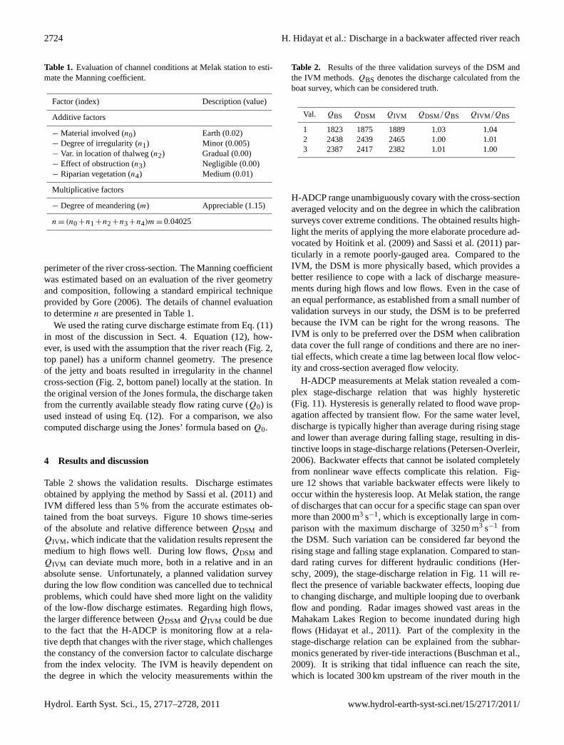
Table 1. Evaluation of channel conditions at Melak station to esti-mate the Manning coefficient.

Factor (index) Description (value)

Additive factors

− Material involved (n0) Earth (0.02)− Degree of irregularity (n1) Minor (0.005)− Var. in location of thalweg (n2) Gradual (0.00)− Effect of obstruction (n3) Negligible (0.00)− Riparian vegetation (n4) Medium (0.01)

Multiplicative factors

− Degree of meandering (m) Appreciable (1.15)

n = (n0+n1+n2+n3+n4)m = 0.04025

perimeter of the river cross-section. The Manning coefficientwas estimated based on an evaluation of the river geometryand composition, following a standard empirical techniqueprovided byGore(2006). The details of channel evaluationto determinen are presented in Table 1.

We used the rating curve discharge estimate from Eq. (11)in most of the discussion in Sect. 4. Equation (12), how-ever, is used with the assumption that the river reach (Fig.2,top panel) has a uniform channel geometry. The presenceof the jetty and boats resulted in irregularity in the channelcross-section (Fig.2, bottom panel) locally at the station. Inthe original version of the Jones formula, the discharge takenfrom the currently available steady flow rating curve (Q0) isused instead of using Eq. (12). For a comparison, we alsocomputed discharge using the Jones’ formula based onQ0.

4 Results and discussion

Table 2 shows the validation results. Discharge estimatesobtained by applying the method bySassi et al.(2011) andIVM differed less than 5 % from the accurate estimates ob-tained from the boat surveys. Figure10 shows time-seriesof the absolute and relative difference betweenQDSM andQIVM , which indicate that the validation results represent themedium to high flows well. During low flows,QDSM andQIVM can deviate much more, both in a relative and in anabsolute sense. Unfortunately, a planned validation surveyduring the low flow condition was cancelled due to technicalproblems, which could have shed more light on the validityof the low-flow discharge estimates. Regarding high flows,the larger difference betweenQDSM andQIVM could be dueto the fact that the H-ADCP is monitoring flow at a rela-tive depth that changes with the river stage, which challengesthe constancy of the conversion factor to calculate dischargefrom the index velocity. The IVM is heavily dependent onthe degree in which the velocity measurements within the

Table 2. Results of the three validation surveys of the DSM andthe IVM methods.QBS denotes the discharge calculated from theboat survey, which can be considered truth.

Val. QBS QDSM QIVM QDSM/QBS QIVM /QBS

1 1823 1875 1889 1.03 1.042 2438 2439 2465 1.00 1.013 2387 2417 2382 1.01 1.00

H-ADCP range unambiguously covary with the cross-sectionaveraged velocity and on the degree in which the calibrationsurveys cover extreme conditions. The obtained results high-light the merits of applying the more elaborate procedure ad-vocated byHoitink et al.(2009) andSassi et al.(2011) par-ticularly in a remote poorly-gauged area. Compared to theIVM, the DSM is more physically based, which provides abetter resilience to cope with a lack of discharge measure-ments during high flows and low flows. Even in the case ofan equal performance, as established from a small number ofvalidation surveys in our study, the DSM is to be preferredbecause the IVM can be right for the wrong reasons. TheIVM is only to be preferred over the DSM when calibrationdata cover the full range of conditions and there are no iner-tial effects, which create a time lag between local flow veloc-ity and cross-section averaged flow velocity.

H-ADCP measurements at Melak station revealed a com-plex stage-discharge relation that was highly hysteretic(Fig. 11). Hysteresis is generally related to flood wave prop-agation affected by transient flow. For the same water level,discharge is typically higher than average during rising stageand lower than average during falling stage, resulting in dis-tinctive loops in stage-discharge relations (Petersen-Overleir,2006). Backwater effects that cannot be isolated completelyfrom nonlinear wave effects complicate this relation. Fig-ure 12 shows that variable backwater effects were likely tooccur within the hysteresis loop. At Melak station, the rangeof discharges that can occur for a specific stage can span overmore than 2000 m3 s−1, which is exceptionally large in com-parison with the maximum discharge of 3250 m3 s−1 fromthe DSM. Such variation can be considered far beyond therising stage and falling stage explanation. Compared to stan-dard rating curves for different hydraulic conditions (Her-schy, 2009), the stage-discharge relation in Fig.11 will re-flect the presence of variable backwater effects, looping dueto changing discharge, and multiple looping due to overbankflow and ponding. Radar images showed vast areas in theMahakam Lakes Region to become inundated during highflows (Hidayat et al., 2011). Part of the complexity in thestage-discharge relation can be explained from the subhar-monics generated by river-tide interactions (Buschman et al.,2009). It is striking that tidal influence can reach the site,which is located 300 km upstream of the river mouth in the



0

500

1000

1500

2000

2500

3000

3500

4000

Q (

m3 s

−1 )

−1000

0

1000

∆Q (

m3 s

−1 )

02−Apr−2008 11−Jul−2008 19−Oct−2008 27−Jan−2009 07−May−2009 15−Aug−2009−0.5

00.5

∆Q/Q

(−

)

IVMDSM

Fig. 10. Continuous series of discharge estimates derived from H-ADCP data with the DSM and the IVM. Central and bottom panels offer acomparison between DSM and the IVM to convert H-ADCP data to discharge, where1Q = QDSM−QIVM .

0 1000 2000 3000 40002

4

6

8

10

Q (m3 s−1)

h (m

)

H−ADCP (IVM)H−ADCP (DSM)Rating curve

Fig. 11. Water stage and discharge estimates at Melak station, ob-tained from a rating curve (Jones’ formula) and from H-ADCP mea-surements. Water stage is with respect to the position of a pressuregauge about 9 m from the deepest part of the river cross-section.

Mahakam delta. At low discharges in August 2009, the tidalsignal is clearly visible in the discharge series. Due to theflat terrain of the middle and lower Mahakam, tidal energypropagates up to the Mahakam lakes area, where much of thetidal energy is dissipated. Subharmonics such as the MSf, anoceanographic term for the fortnightly constituent of the tidecreated by nonlinear interaction of the tides induced by theMoon and the Sun with the river discharge, may extend be-yond the lakes region. However, this effect cannot be readilyisolated from river discharge variation as discharge variationfeatures fortnightly variation both in the presence and in ab-sence of a tidal influence.

0 500 1000 1500 2000 2500 30004

5

6

7

8

9

10

Q (m3 s−1)

h (m

)

H−ADCP (IVM)H−ADCP (DSM)Rating curve

28 June

24 May

Fig. 12. Water stage versus discharge for the period between24 May–28 June 2008. Multiple loops and discharge oscillations in-dicate variable backwater effects also occurred within the hysteresisloop.

The wide loops in the stage-dischage plot are the resultof the geographical complexity of the region where Melakstation is located, experiencing a flashy discharge from up-stream and backwater effects from downstream. The flashydischarge regime relates to high rainfall rates in large parts ofthe catchment upstream of Melak, which dominates the mod-erating effect of the rain forest. The backwater effects arecaused both by the lakes and a number of tributaries, all af-fecting the water level profile. Lake emptying and filling pro-cesses contribute to retarding and accelerating the river flow



19−May−2008 29−May−2008 08−Jun−20080

1000

2000

3000Q

(m

3 s−

1 )

0

2

4

6

8

10

h (m

)

29−Oct−2008 08−Nov−2008 18−Nov−20080

1000

2000

3000

Q (

m3 s

−1 )

0

2

4

6

8

10

h (m

)

Q Melakh Melakh Lake Jempangh Muara Kaman

Fig. 13. Water stage and discharge during lake emptying (top) andduring lake filling (bottom). Muara Kaman, where the tidal signalwas observed during most of the measurement period, is locateddownstream of the Mahakam lakes area about 170 km from Melak.

velocity. Figure13illustrates the lake emptying and lake fill-ing influencing water levels and discharge upstream. At thestart of lake emptying, when the lake level was still high,water stage in Melak was relatively high for a relatively lowdischarge. When the lake level dropped, the backwater effectwas reduced and discharge increased while water stage keptdecreasing until the point that discharge was sufficiently highto make water stage follow the trend in the discharge time-series. The opposite mechanism took place during lake fill-ing as shown in Fig.13 (bottom panel). Water stage recordsdownstream of the Mahakam lake area (Muara Kaman) indi-cate that some peaks of water level were shaved by the lakefilling and emptying mechanism.

The discharge obtained from the stage-discharge relationusing Jones formula is merely a rough estimate of dischargeat Melak station, indicating the range of discharge variation.It did not capture the detailed discharge dynamics as revealedby the H-ADCP measurements. This can be related to a widevariety of reasons. The Froude number takes a value around0.01, which likely indicates the inertial term in the momen-tum equation to be negligible. A non-dimensional version ofthe St. Venant equations directly shows that the inertial termsdrop out for small values of the Froude number (Pearson,1989). The key assumption used to derive the Jones formulais the applicability of the kinematic wave equation to deal

500 1000 1500 2000 2500 3000 3500500

1000

1500

2000

2500

3000

3500

QJ−Qsteady RC

(m3 s−1)

QJ−

Qki

nem

atic (

m3 s

−1 )

Fig. 14. Comparison of discharge estimates obtained using theJones formula based onQkin (uniform channel geometry assump-tion) and those based onQ0 (discharge taken from the steady flowrating curveQ0 = 125.98× (h+1.5)1.256) for the whole observa-tion period. The small deviation confirms that the two approachesyield similar results. Only during peak discharges, the use ofQ0instead ofQkin can result in slightly different rating curve-basedestimates of the discharge.

with the surface gradient term in the non-inertial wave equa-tion. Although this approach can be successful under certainbed slope and flow conditions (Pearson, 1989; Perumal et al,2004; Dottori et al., 2009), the kinematic wave equation can-not capture discharge dynamics in backwater affected riverreaches (e.g.,Tsai, 2005). The stage-discharge relation isonly expected to be applicable if the channel geometry is uni-form. The top panel in Fig.2 shows there is some irregularityin the cross-section, related to the low flow velocities beneaththe jetty. Therefore, the complexity of the stage-dischargeplot can be partly explained from the non-uniformity of thechannel geometry. Figure14 shows the comparison of dis-charge estimates obtained using the Jones formula basedon Qkin (uniform channel geometry assumption) and thosebased onQ0 (discharge taken from the steady flow ratingcurve). During peak discharges, the use ofQ0 instead ofQkin can result in slightly different rating curve-based esti-mates of the discharge. Out-of-bank spills and return flowsfrom flood plains occurring in the study area during the pe-riod of flood peak could also be among possible reasons forthe failure of the Jones formula to adequately predict flooddynamics. The Jones formula is just one of a series of formu-las available to predict discharge from time-series of a singlelevel gauge (Henderson, 1966; Di Silvio, 1969; Fread, 1975;Lamberti and Pilati, 1990; Perumal and Ranga Raju, 1999),all aiming to improve the original Jones’ formula.Dottoriet al.(2009) explicitly mentions that they are best applicablewhen flow conditions are quasi kinematic. Backwater effectsrender the kinematic wave assumption invalid, hence none



of these approaches will be capable of reproducing the wideloops occurring at Melak station, which underlines the im-portance of monitoring additional information besides stageat a single section. Considering the ease of deployment ofH-ADCPs, they offer a promising alternative to measure dis-charge.

5 Conclusions

Flow measurements using a 600 kHz H-ADCP were carriedout at a 300 m wide cross section of the Mahakam River inMelak, 40 km upstream of the Mahakam lakes area. Con-ventional boat-mounted ADCP measurements were periodi-cally taken to establish water discharge through the cross sec-tion. We followed a recently developed semi-deterministic,semi-stochastic method (DSM) to convert the H-ADCP todischarge, and compared the results with those obtainedfrom the index-velocity method (IVM) and a rating curvemodel. The DSM method was found to be comparable withthe IVM, the difference with discharge estimates from theboat-mounted ADCP surveys was less than 5 % based onthree validation surveys. The continuous time-series of dis-charge showed that the validation data were representativefor medium to high flows. A stage-discharge model basedon Jones’s formula captured only a small portion of the dis-charge dynamics, which was attributed to the invalidity of thekinematic wave assumption due to backwater effects. A dis-charge range of about 2000 m3 s−1 was established for a par-ticular stage in the recorded discharge series, which is about60 % of the peak discharge and therefore exceptionally large.The large range of discharge occurring for a given stage wasattributed to multiple backwater effects from lakes and tribu-taries, floodplain impacts and effects of river-tide interaction,which generate subharmonics that cannot readily be isolatedfrom river discharge oscillations.

Acknowledgements.This research has been supported by theNetherlands organisation for scientific research, under grantnumber WT 76-268. The help from Fajar Setiawan and UnggulHandoko (LIPI – Research Centre for Limnology) and DavidVermaas (Wageningen University) in data collection is gratefullyacknowledged. The authors appreciate comments and suggestionsfrom the three reviewers that helped improve the manuscript.

Edited by: G. Di Baldassarre

References

Beven, K. J.: Rainfall-runoff modelling: the primer, John Wiley &Sons, Chichester, England, 2001.

Buschman, F. A., Hoitink, A. J. F., van der Vegt, M.,and Hoekstra, P.: Subtidal water level variation controlledby river flow and tides, Water Resour. Res, 45, 1–12,doi:10.1029/2009WR008167, 2009.

Di Baldassarre, G. and Montanari, A.: Uncertainty in river dis-charge observations: a quantitative analysis, Hydrol. Earth Syst.Sci., 13, 913–921,doi:10.5194/hess-13-913-2009, 2009.

Di Silvio, G.: Flood wave modifications along prismatic channels,J. Hydraul. Div. ASCE, 95, 1589-1614, 1969.

Dottori, F. and Todini, E.: Reply to Comment on “A dynamic rat-ing curve approach to indirect discharge measurement by Dottoriet al. (2009)” by Koussis (2009), Hydrol. Earth Syst. Sci., 14,1099–1107,doi:10.5194/hess-14-1099-2010, 2010.

Dottori, F., Martina, M. L. V., and Todini, E.: A dynamic ratingcurve approach to indirect discharge measurement, Hydrol. EarthSyst. Sci., 13, 847–863,doi:10.5194/hess-13-847-2009, 2009.

Fread, D. L.: Computation of stage-discharge relationship affectedby unsteady flow, Water Resour. Bull., 12, 429-442, 1975.

Godin, G. and Martı́nez, A.: Numerical experiments to investigatethe effects of quadratic friction on the propagation of tides in achannel, Cont. Shelf Res., 14, 723–748, 1994.

Gordon, R. L.: Acoustic measurement of river discharge, J. Hy-draul. Eng., 115, 925–936, 1989.

Gore, J. A.: Methods in Stream Ecology, chap. Discharge Measure-ments and Streamflow Analysis, Academic Press, 51–77, 2006.

Henderson, F. M.: Open channel flow, Prentice Hall, 544 pp., 1966.Herschy, R. W.: Streamflow Measurement, Taylor & Francis, Lon-

don and New York, 3rd Edn., 2009.Hidayat, Hoekman, D. H., Vissers, M. A. M., and Hoitink, A. J. F.:

Combining ALOS-PALSAR imagery with field water level mea-surements for flood mapping of a tropical floodplain, Proceed-ings of the International Symposium on LIDAR and Radar Map-ping: Technologies and Applications, Nanjing, China, in press,2011.

Hoitink, A. J. F., Buschman, F. A., and Vermeulen, B.: Continuousmeasurements of discharge from a horizontal acoustic Dopplercurrent profiler in a tidal river, Water Resour. Res, 45, 1–13,doi:10.1029/2009WR007791, 2009.

Jones, B. E.: A method of correcting river discharge for a changingstage, US Geological Survey Water Supply Paper, 375-E, 117-130, 1916.

Koussis, A. D.: Comment on “A praxis-oriented perspective ofstreamflow inference from stage observations – the method ofDottori et al. (2009) and the alternative of the Jones Formula,with the kinematic wave celerity computed on the looped ratingcurve” by Koussis (2009), Hydrol. Earth Syst. Sci., 14, 1093–1097,doi:10.5194/hess-14-1093-2010, 2010.

Lamberti, P. and Pilati, S.: Quasi-kinematic flood wave propaga-tion, Meccanica, 25, 107–114, 1990.

Le Coz, J., Pierrefeu, G., and Paquier, A.: Evaluation of river dis-charges monitored by a fixed side-looking Doppler profiler, Wa-ter Resour. Res., 44, 1–13,doi:10.1029/2008WR006967, 2008.

McMillan, H., Freer, J., Pappenberger, F., Krueger, T., and Clark,M.: Impacts of uncertain river flow data on rainfall-runoffmodel calibration and discharge predictions, Hydrol. Process.,24, 1270–1284,doi:10.1002/hyp.7587, 2010.

Moore, S. A., Le Coz, J., Hurther, D., and Paquier, A.: Backscat-tered intensity profiles from horizontal acoustic Doppler cur-rent profilers, in River Flow 2010, Bundesanstalt fur Wasserbau,Braunschweig, Germany, 1693–1700, 2010.

Nihei, Y. and Kimizu, A.: A new monitoring system for river dis-charge with horizontal acoustic Doppler current profiler mea-surements and river flow simulation, Water Resour. Res., 44, 1–


http://dx.doi.org/10.1029/2009WR008167

http://dx.doi.org/10.5194/hess-13-913-2009



http://dx.doi.org/10.1029/2009WR007791


http://dx.doi.org/10.1029/2008WR006967

http://dx.doi.org/10.1002/hyp.7587


15, doi:10.1029/2008WR006970, 2008.Pearson, C. P.: One-dimensional flow over a plane: Criteria for

kinematic wave modelling, J. Hydrol., 111, 39–48, 1989.Perumal, M. and Ranga Raju, K. G.: Approximate convection-

diffusion equations, J. Hydrol. Eng., 4, 160–164, 1999.Perumal, M., Shrestha, K. B., and Chaube, U. C.: Reproduction of

Hysteresis in Rating Curves, J. Hydrol. Eng.-ASCE, 130, 870-878, 2004.

Petersen-Overleir, A.: Modelling stage-discharge relationships af-fected by hysteresis using the Jones formula and nonlinear re-gression, Hydrol. Sci. J., 51, 365–388, 2006.

Petersen-Overleir, A. and Reitan, T.: Bayesian analysis ofstage-fall-discharge models for gauging stations affectedby variable backwater, Hydrol. Process., 23, 3057–3074,doi:10.1002/hyp.7417, 2009.

Sassi, M. G., Hoitink, A. J. F., Vermeulen, B., and Hidayat: Dis-charge estimation from H-ADCP measurements in a tidal riversubject to sidewall effects and a mobile bed, Water Resour. Res.,47, W06504, 1–14,doi:10.1029/2010WR009972, 2011.

Schmidt, A. R.: Analysis of stage-discharge relations for open-channel flows and their associated uncertainties, PhD the-sis,University of Illinois, available at:https://netfiles.uiuc.edu/aschmidt/www/ARSThesis/ARSThesis.htm(last access: 9 Au-gust 2011), 2002.

Simpson, M. R. and Bland, R.: Methods for accurate estimation ofnet discharge in a tidal channel, IEEE J. Oceanic Eng, 25, 437–445, 2000.

Tsai, C. W.: Flood routing in mild-sloped rivers – wave characteris-tics and downstream backwater effect, J. Hydrol., 308, 151–167,doi:10.1016/j.jhydrol.2004.10.027, 2005.

van Gerven, L. P. A. and Hoitink, A. J. F.: Analysis of river plan-form geometry with wavelets: application to the Mahakam Riverreveals geographical zoning, in: Proceedings of RCEM, 2009.

Yen, B. C. and Tsai, C. W. S.: On noninertia wave versus diffusionwave in flood routing, J. Hydrol., 244, 97–104, 2001.


http://dx.doi.org/10.1002/hyp.7417

http://dx.doi.org/10.1029/2010WR009972

https://netfiles.uiuc.edu/aschmidt/www/ARS_Thesis/ARS_Thesis.htm

https://netfiles.uiuc.edu/aschmidt/www/ARS_Thesis/ARS_Thesis.htm

Documents

Discharge estimation in a backwater affected meandering river