2016 ANNUAL

AGRICULTURAL OUTLOOK

Coordinated by Jim Hilker

Staff Paper 2016-01 February, 2016

Department of Agricultural, Food, and Resource Economics MICHIGAN STATE UNIVERSITY East Lansing, Michigan 48824

MSU is an Affirmative Action/Equal Opportunity Institution

Staff Paper

2016 Annual Agricultural Outlook

Coordinated by:

Jim Hilker hilkerj@msu.edu

31 pages

Copyright 2016 by James H. Hilker. All rights reserved. Readers may make verbatim copies of this document for non-commercial purposes by any means, provided that this copyright notice appears on all such copies.

TABLE OF CONTENTS Page

THE GENERAL ECONOMY: 2016 John Whims ......................................................................................................................... 1 POLICY AND TRADE OUTLOOK David Schweikhardt .............................................................................................................. 5 2016 INPUT COSTS Bill Knudson and John Whims ............................................................................................... 8 MICHIGAN AGRICULTURAL LAND PRICE OUTLOOK Christopher Wolf and Eric Wittenberg ................................................................................. 10 2016 ANNUAL CROPS OUTLOOK Jim Hilker .............................................................................................................................. 11 2016 ANNUAL LIVESTOCK OUTLOOK Jim Hilker .............................................................................................................................. 20 2015 DAIRY SITUATION AND OUTLOOK Christopher Wolf .................................................................................................................. 23 TAXES IN 2015 AND 2016 Larry Borton and John Jones ................................................................................................ 26 FARM INCOME David Schweikhardt .............................................................................................................. 29

1

THE GENERAL ECONOMY: 2016 John Whims U.S. Economy What a difference a year makes. Who could have forecasted the implosion of the energy sector at the start of 2015? Oil prices fell from over $100.00 per barrel in January 2015 to below $40.00 / barrel at the close of the year, down over 60%! While the Federal Reserve Bank (FED) decided to finally raise rates for the first time in a decade keeping much of the financial world guessing for most of the year as to when it might finally happen. At the end of the year, global stock markets began to gyrate wildly which has carried over in to 2016, weighed down by the uncertainty created by news of China’s slowing economy and continued oil price weakness. Moving forward, increased volatility is likely to be a hallmark of the U.S. economy in 2016. In general, the economy is still relatively strong (at least compared to most other countries); we are, however, likely in the mid-stage phase of the business cycle. This usually portends greater uncertainty for an economy; we are likely no longer in the boring “status quo” mode of operation. Historically, the FED initiates rate hikes during the mid-stage phase of a business cycle, where it coincides with a broadening U.S. expansion. Based on FED Committee comments in December 2015; they believe their indicators show that “economic activity has been expanding at a moderate pace.” The foundation of this thesis is grounded on their perspectives/observations that; (1) household spending is healthy; (2) business fixed investment has been increasing at solid rates; and (3) the housing sector is showing signs of significant life. The combination of these factors was enough for the Committee to raise rates at the end of 2015. At the end of the day, the FED is concerned with assessing the path and magnitude of the economy in order to balance the two objectives of maximum employment and price stability (2.0% inflation) in the economy. The FED views the recent strength the labor market, i.e., a tightening of the supply of labor and the pressure for higher wages as a precursor to increased inflation. The FED must weigh the available current economic data points along with future/forecasted economic data as they formulate their monetary policies. They have already telegraphed their inclination towards multiple rate hikes in 2016 (potentially as many as three). But is this the direction that we actually think the U.S. economy is headed in 2016, such that it will warrant as many as three rate hikes? Here is what we think going forward: GDP: Most macro economists are forecasting real GDP of 3.0% or higher for 2016. In our estimation, real GDP will be lower, in the 2.0% to 2.5% range (which still isn’t bad). The consumer and their spending will generate most of the growth with very little help from the rest of the economy. Headwinds will be felt in a number of key areas in the economy:

The U.S. export market will remain weak as the dollar stays strong against most other global currencies.

Government spending will be restricted in an election year where there will be absolutely no incentive to raise taxes.

The energy complex will continue to face significant financial challenges such that little or no capital investments will be transacted, despite that fact that oil prices will probably firm by the end of the year.

2

Inflation: Core inflation (excluding food and energy) has been exceedingly tame over the last three years, averaging 1.7%. Headline inflation (food, energy, and everything else) has definitely been pacified especially with the radical decline in global energy prices. Energy prices will likely firm modestly in 2016, and coupled with upward pressure on worker wages should push headline inflation towards 2.5% by the end of the year. Watch to see if OPEC is actually able to agree upon any supply reductions, or if any geopolitical unrest trims oil supplies as well; this could push inflation even higher towards 3.0%, something we haven’t seen in quite a while. Interest Rates: Interest rates are perhaps the absolute single most difficult macro variable to forecast. Going into 2016, the bias is certainly to the upside, the question is by how much? The benchmark 10-Year Treasury averaged 2.2% in 2015. Bond yields should typically be a function a normalized spread above inflation, which is generally around 1.5%. Given our forecast of headline inflation nearing 2.5%, coupled with a spread of 1.5% that would put the 10-Year near 4.0% by the end of the year. What is likely to happen, however, is the global push towards greater monetary easing, think of the European Central Bank (ECB) and their new quantitative easing program and China as they move to devalue their currency to prop up their economy and stock market. These programs will likely keep the 10-Year closer to 3.5% in reality.

Unemployment: Employment growth will continue in 2016, thus driving down the unemployment rate to 4.7%. Most all new jobs created will be in the service and professional industries versus the government and manufacturing industries. Employment should grow by approximately 1.9% (220,000 average new jobs per month), slightly below the GDP forecast of 2.25%, which reflects continued modest productivity gains of office and factory workers. Note: the combination of retiring baby boomers, teens staying in school longer and the misalignment of skills and wages have resulted in potential workers dropping out of the job market, this has driven the unemployment level down even further than expected and will persist in 2016, as well.

Something to Watch: Corporate leverage has reached a 12-year high as displayed by the debt-to-earnings ratio, (see Figure 2). This is a global phenomenon where one in three corporations are failing to generate high enough returns on investments to cover their respective cost of funding. This means that there is little margin for error for many corporations especially if earnings begin to stall because of any kind of future economic contraction. Much of the cheap credit accumulated by companies during the FED’s quantitative easing programs has gone to Mergers and Acquisitions binges, fund share buyback programs and dividend payments versus monies being spent on long-run investments.

3

Figure 1: Corporate Leverage is Rising

Michigan Economy Michigan continues to see positive growth in its economy heading into the sixth year of recovery since the summer of 2009. The foundation for this growth thesis remains in place for 2016. Last year, Michigan jobs grew in the first quarter by an annualized rate of 3.8% and ultimately averaged 1.4% for the year. Job growth should continue at this 1.4% annualized rate for the first three quarters of 2016 and increase to a 1.6% annualized rate in the fourth quarter. In due course, the forecasted job gains should lead to an increase of 61,000 in 2016, while laying the groundwork for expansion of jobs heading into 2017. If jobs expand by the forecasted amounts in 2016 and 2017, that will take Michigan employment back to the same level as spring 2003. The new jobs being created continue to occur in the professional and business services sectors (25% of the total, with 60% being in the professional, scientific, and technical subgroup, highly skilled) and trade, transportation and utilities (20% of the total). Reemergence of the housing sector is leading to more jobs in construction, as 1 in 6 new Michigan jobs are being linked to the expansion in residential construction.

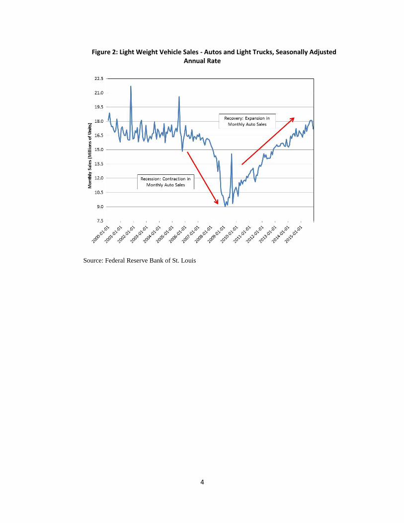
Coming out of the recession in 2009, growth in Michigan manufacturing jobs were crucial to healing the State’s economy; now, however, it is forecasted that only one in 12 jobs created over the next two years will be in manufacturing. Despite most of the new Michigan job growth occurring in the non-manufacturing sectors of the economy, the general well-being of the auto industry is still incredibly important to the state’s overall economy. The industry has recovered significantly since the recession bottom in 2009, as highlighted by the increase in auto and light truck sales (see Figure 2).

The U.S. Bureau of Labor Statistics estimated in November 2015 (latest survey results)

that Michigan employed 175,600 workers in the motor vehicles and motor vehicle parts manufacturing sectors (not including the wholesale and retail sectors). The continued low interest rate environment and upward pressure on increased worker wages and salaries should translate into modestly higher auto sales; this is good news for Michigan. U.S. auto and light truck sales are expected to increase from 17.4 million units in 2015, to 18.1 million units in 2016, up just over 4.0%. Sales growth is being driven heavily by light truck sales, which include sport utility vehicles (SUV’s) and compact utility vehicles (CUV’s), by the end of 2017 light truck sales will account for almost 58% of total sales of light vehicles.

4

Figure 2: Light Weight Vehicle Sales - Autos and Light Trucks, Seasonally Adjusted Annual Rate

Source: Federal Reserve Bank of St. Louis

5

POLICY AND TRADE OUTLOOK David B. Schweikhardt

Total U.S. agricultural exports are projected to be $131.5 billion in Fiscal Year 2016 (the October 2015 to September 2016 period). This level of exports would be an $8.2 billion decrease from FY 2015 and a $19.8 billion decrease from the record high registered in FY 2014. This decrease in value was the result of both lower prices for exports and a lower volume of products exported. This weakness in exports is expected to be driven by slow economic growth on a worldwide basis, the continued strength of the U.S. dollar, and favorable stock levels in most producing countries. The USDA’s last outlook report for agricultural trade was released in November 2015, but several signs emerged in the late 2015 and early 2016 that confirm a continuation this outlook. Only a major disruption caused by weather would be likely to change this outlook. U.S. Agricultural Trade Outlook

The projected 2016 decrease in total U.S. agricultural exports represents a decrease in both export price and volume for most categories of products. Among the major product categories, only exports of horticultural products are projected to increase. A major change in recent years is that horticultural products now represent the largest single category of U.S. agricultural products, replacing the traditional leader of grains and feeds. Horticultural product exports (both fresh and processed) are projected to be reach $36.5 billion in 2016, an increase of $2.4 billion over 2015. This trend continues to signal a significant transformation in the composition of U.S. agricultural exports. Namely, the rapid growth in worldwide consumer demand for horticultural products, including U.S. products, continues to contribute to growth in exports of horticultural products.

Exports of grains and feeds are projected at $28.6 billion in 2016, a decrease of $3.0

billion from 2015, with both corn (-$400 million) and wheat (-$500 million) expected to decrease during 2016. Oilseeds and products (-$5.4 billion from $31.7 billion in 2015), livestock products (-$700 million from $18.2 billion) are also expected to decrease in 2016. In the livestock category, beef exports are expected to decrease by $200 million to $5.6 billion, while pork exports are expected to decrease by $500 million to $4.4 billion. Poultry product exports are projected to decrease by $200 million to $5.2 billion, and dairy product exports are expected to increase by $100 million to $5.6 billion. Only wheat, soybean oil, and soybean meal are expected to show minor increases in export volume.

The destination of U.S. exports continues its recent pattern. In 2016, Asia will be the

leading U.S. agricultural export destination (with China and Japan as the leading buyer of U.S. export products in the region at $42.5 and $11.2 billion, respectively). China’s purchases from U.S. agriculture are projected to be $5.4 billion lower in 2016, giving an indication of the importance of China’s economic growth on U.S. producers’ exports. Canada’s ($21.3 billion) and Mexico’s ($18.0 billion) purchases of U.S. agricultural exports are expected to remain unchanged in 2016. A major uncertainty for 2016 is the impact of the U.S.-Canadian exchange rate on U.S. exports. In past year, the Canadian dollar has suffered a severe depreciation against other currencies as a result of the decline in oil prices. The U.S.-Canadian exchange rate changed from parity (1:1) in June 2011 to 93¢ U.S. per Canadian dollar in June 2014 to 70¢ U.S. per Canadian dollar in January 2016. This depreciation of the Canadian dollar has contributed to a major issue

6

of food price inflation in Canada in recent months and could reduce U.S. exports to Canada, particularly for fruits and vegetables.

Total U.S. agricultural imports are projected to increase to $122 billion in 2016, a level

$8 billion higher than the record level of 2015. Horticultural product imports are expected to experience the largest change, with an increase of $4.9 billion to a projected total of $54.5 billion. The second largest category of imports is projected to be sugar and tropical products with $27.2 billion in imports (including $14.8 billion in imports of cocoa, coffee, and rubber). Canada ($23.8 billion), Mexico ($21.8 billion) and the European Union ($20.9 billion) are projected to continue as the three largest suppliers of U.S. agricultural imports. As is the case with U.S. exports, changing consumer preferences are leading to a transformation of the type of food products that are being imported into the United States. Fresh and processed fruit ($17.2 billion), fresh and processed vegetables ($11.6 billion), wine and beer ($10.7 billion), and coffee ($7.3 billion) constitute the largest U.S. imports of agricultural and food products.

Farm Bill Implementation

The Agricultural Act of 2014 provided farmers with two alternative risk management programs. The Price Loss Coverage program (PLC) provides a payment when the effective price (national average market price) is below the PLC reference price ($3.70 for corn, $8.40 for soybeans, and $5.5 0 for wheat). The second choice, the Agricultural Risk Coverage (ARC) program provides payments when the actual revenue (calculated on a county or individual basis) for a crop is less than the ARC guarantee for that crop. Producers were required to make a one-time election of either PLC or ARC for the 2014-18 crop years. The ARC and PLC programs replaced the Direct and Countercyclical Payment program included in the 2008 farm bill.

The replacement of the DCP program with the ARC/PLC programs will be important for

2016 and the following years. Given the existing outlook for lower commodity prices, the ARC/PLC programs will provide a much more effective safety net for farm income that the DCP programs would have provided under existing conditions. In January 2016, the Congressional Budget Office (CBO) projected that expenditures on ARC and PLC for Fiscal Year 2016 (October 2015 to September 2016) will total $4.9 billion (including $3.4 billion in ARC payments for corn, $297 million for soybeans and $326 million for wheat). In Fiscal Year 2017, budget expenditures for ARC and PLC are expected to increase to $6.1 billion.

This expenditure, which is a “shock absorber” against falling commodity prices, is

significantly greater than would have been spent under the DCP program. It should also be noted that the commodity prices used in the CBO projections may prove to be higher than will be witnessed in 2016-2017. If so, the expenditures on ARC and PLC will be higher than projected in the CBO report and their impact on farm income will be even greater than projected. In any case, the existing economic environment for agriculture will provide a key test of the workability and effectiveness of the programs contained in the Agricultural Act of 2014.

Trade and Domestic Policy Issues

With the completion of negotiations on the TransPacific Partnership (TPP) agreement, the next step in the TPP process would be the approval or disapproval of the agreement by Congress. This trade agreement reduces trade barriers (tariffs and quotas) on all products,

7

including agriculture, over a 30-year period. The 11 countries included in the agreement include the United States, Australia, Brunei Darussalam, Canada, Chile, Japan, Malaysia, Mexico, New Zealand, Peru, Singapore, and Vietnam. These countries represented the markets for over 60% of total U.S. agricultural exports in 2015. In addition, because agricultural trade barriers tend to be higher than trade barriers on most industrial products, an agreement reducing such barriers is likely to have a larger impact on agricultural exports than on other industries. The debate in Congress over TPP is expected to be contentious, and the agreement cannot be passed without votes from both parties. In addition, many of the newer members of Congress have never voted on a major trade agreement, leaving greater uncertainty about the likely direction of their votes. Though the Obama administration is likely to prefer that a vote be taken sometime this year, some Congressional observers have concluded that a vote is very unlikely until sometime after the 2016 election.

8

2016 INPUT COSTS Bill Knudson and John Whims Summary

Agricultural commodity prices have generally trended downward in 2015. Similarly, after several years of increases, input prices have now seen a pullback; this is particularly true for those agricultural inputs that are linked to the energy complex (oil and natural gas), such as fertilizer and diesel. Current diesel prices are now the lowest they have been since March 2009, and there does not appear to be to be any reason to believe that they will rise meaningfully any time soon. Interest rates will remain historically low, however, the Federal Reserve Bank made its first rate increase at the end of 2015, in almost ten years! Despite the anticipated path of persistent historical low rates in 2016, many Michigan farmers, however, may continue to experience difficulty in accessing credit. Farmer profitability and profit margins came under pressure in 2015 and will they will likely stay that way in 2016, making for another year of tight credit. While most commodity and input prices worked their way lower in 2015, so far seed prices for corn have remained firm, heading into 2016; however, prices may actually come under slight pressure in 2016, given the profitability headwinds being felt by crop farmers. Fertilizer

After rising for several years’ fertilizer prices have finally started to decline. According to the USDA, the price of anhydrous ammonia in Illinois averaged $578 a ton early January 2016, a decrease of 20.3% from January 2015. Similarly, the price of urea was $370 a ton, a decrease of 10.2%, MAP averaged $504 a ton, a decline of 12.0% and potash averaged $368 ton, a decrease of 22.7%, year-over-year.

There are two other issues to consider when examining these figures. The first consideration is that prices are likely to seasonally rise in the spring as farmers make their purchases as planting season approaches and secondly, that these figures are for Illinois. Prices in Michigan may vary somewhat to the Illinois reference prices that the USDA collects, such that Michigan prices might be higher given the addition of transportation costs to the base prices observed in Illinois. Seed

Seed prices appear to be steady. In September 2015, Purdue University estimated the per acre cost of soybean seed to be $74, a decline of $1 from the 2014 estimate; the per acre cost of corn seed is estimated to be $123, also a $1 decline from the 2014 estimate; and the per acre cost of wheat seed is estimated to be $44, which is unchanged from the previous estimate. There have been downward pressures on corn and soybean commodity prices which usually portends lower seed prices. Fuel

Oil prices have fallen dramatically since the record high of $145/barrel in July 2008 (see Figure 2). Since the record high, prices have fallen over 80%, breaking $30/barrel for the first time since 2003. According to the U.S. Energy Information Administration, reported Midwest

9

retail price of diesel was $2.10 in January 2016. This is 91 cents a gallon or 30.2% lower than the previous year. While there is long-term uncertainty with respect to fuel prices, in the short-run it appears that there will be little upward pressure on diesel prices throughout most of 2016.

Figure 3: West Texas Intermediate – Cushing, Oklahoma - Crude Oil, Spot Price

Source: U.S. Energy Information Administration (EIA)

Interest Rates

Interest rates remained low throughout 2015, and will likely remain historically low in 2016. According to the Federal Reserve Bank of Chicago, interest rates in the region which includes the Lower Peninsula, most of Indiana and Illinois, Iowa and the southern and western part of Wisconsin, were 4.82% for operating loans and 4.58% for real estate loans in the third quarter of 2015. Interest rates for farm loans have declined by 0.05% for operating loans and 0.04% for real estate loans from the third quarter of 2015.

Interest rates are likely to remain low, but have an upward bias in 2016. The Federal Reserve Bank (FED) increased its lending rate by 0.25% in late 2015, and has telegraphed the likelihood of future rate hikes in 2016 (potentially as many as three) as some modest signs of core inflation (excluding energy) begin to emerge. There are, however, numerous economic clouds on the horizon that could alter the FED’s thesis for the need to raise rates in 2016. Major developing economies such as China/Brazil/Russia are in varying degrees of recessions, while Japan and much of Europe are having estimates of their economic output (Gross Domestic Product, GDP) revised downward as they show signs of being in the later stages of their respective business cycles.

10

MICHIGAN AGRICULTURAL LAND PRICE OUTLOOK Christopher Wolf and Eric Wittenberg

Lower field crop returns in 2015 placed downward pressure on farmland values. Corn Belt states in particular, such as Illinois and Indiana, report cropland prices declining 5% or more. Michigan respondents reported either flat land prices or a small decrease in 2015 compared to 2014. In addition to expected returns, interest rates are a major influence on land prices. The low interest rates of recent years have supported higher farmland values. In addition, Michigan has crops with returns that are not necessarily correlated with corn and soybeans such as sugar beets and fruit.

To examine the reported land prices we calculate the capitalized value of the land using a simple model. The capitalized value of land is the income divided by discount rate which is essentially the interest rate here. We use reported cash rent for income and the 10 year Constant Maturity Treasury (CMT) from the Federal Reserve as the discount rate. Land price for tiled cropland in Michigan’s southern peninsula and capitalized value are reported in the figure. When land price is above capitalized value the price is either too high or there are expectations of future increases in returns or lower interest rates. The figure reveals this was the case in Michigan from 1999 to 2008. When the capitalized value is greater than the land price, which has been the case since 2010, either land prices are not overvalued, the income in the period (i.e., cash rent here) is not viewed as permanent, or there are expectations of higher interest rates.

There are many factors that influence agricultural land values in Michigan and differences in opinion can result in market values not adjusting as our simple model suggests. However, it seems likely that the average farmland price will decline a small percentage with larger declines likely if interest rates increase in 2016.

Reported Tiled Land Price in Michigan Southern Peninsula and Capitalized Value

11

2016 ANNUAL CROPS OUTLOOK Jim Hilker CORN

The 2016 annual Corn Outlook presented here will include the 2015-16 and 2016-17 corn marketing years; the baseline numbers are presented in Table 1. By baseline, I mean, given what I know and expect to date, we all know a lot can and will happen to change these expectations. How the world GDP growth, value of the dollar, oil/gas prices, U.S. and world weather crisis, etc., etc., change from expectations will all play a role, as to a large degree they are all unknowns.

While I still expect price volatility to be higher than pre-2007, with the large U.S.

carryover in 2014-15, the rest of the world having a large carryovers, and the large expected U.S. carryovers expected for 2015-16 and 2016-17, I expect volatility to be down relative to 2006-07 through 2013-14, and the market is reflecting this. At this point, the market is projecting a 54% chance that December 2016 corn futures will be below today’s $3.90 per bushel, and a 60% chance that December 2016 corn futures will be between $3.20 and $4.50 per bushel at harvest. Or, to put another way, there is a 20% chance December 2016 corn futures will be below $3.20 per bushel, and a 20% chance the December 2016 corn futures could be above $4.50 per bushel come harvest time. You need to adjust these for your local basis.

2015-16

U.S. Corn producers planted 88 million acres of corn for the 2015 crop, 1.2 million less acres than intended due to a wet planting season. But then the weather turned pretty good for much of the Corn Belt. Acres harvested for grain came in at 80.7 million acres. The average corn yield for the U.S. was the second highest on record at 168.4 bushels per acre, 4-6 bushels per acre above the trend yield. Multiplying the 168.4 bushel per acre yield by the 80.7 million harvested acres put corn production 13,601 million bushels, 615 million bushels less than last year on 2.6 million less acres. When you add beginning stocks, production, and imports, total supply is projected to be 15,372 million bushels, only 107 million fewer than the record supply set the previous year.

Michigan planted 2.350 million acres of corn in 2015; 200,000 less acres than 2014, and

100,000 acres below the March Prospective Planting Report. Michigan harvested for grain corn acres were 2.070 million, down 140,000 acres from the previous year. Michigan’s average 2015 state yield was a record 162 bushels per acre, one bushel higher than the record 2014 yield, and third record yield in a row. Michigan corn for grain production was a record 355.340 million bushels, the third largest after the previous two years.

U.S. feed use and residual is expected to be 5,300 million bushels, just below last year.

Beef production is expected to be up over 2%, pork production is expected to be up a little, poultry production is expected to be up nearly 2%, and milk cow numbers are expected to remain about the same. Residual use is expected to be lower than 2014-15, which accounts for the small reduction in Feed and Residual despite more livestock production.

12

Food, seed, and industrial uses are projected at 6,570 million bushels for 2015-16. Seed use is expected to be up a little as a few more acres of corn will be planted this spring. Corn used for food and industrial uses, other than ethanol, is expected to grow a bit on population growth. Corn projected to be used for ethanol and DDG’s is 5,200 million bushels, about the same as 2014-15. Low gas prices will limit profits and will likely limit growth.

Exports in 2015-16 are expected to drop-off nearly 9% as the world has plenty of corn,

world growth is weak, and the U.S dollar is expected to stay strong. Total 2015-16 U.S. use is expected to be 13,570 million bushels, down 1.3% from 2014-15. When we subtract total use from total supply we end up with more than ample ending stocks of 1,802 million bushels. Ending stocks as a percent of use would be 13.3%, compared to 12.6% in 2014-15 and 7-9% the previous three years, giving us a projected weighted average season price of $3.60 for 2015-16. See Table 1.

2016-17

My baseline projections for the 2016-17 corn marketing year are shown in Table 1 as well. I am projecting planted 2016 corn acres at 89.3 million acres, up 1.3 million acres from last year, but about the same as farmers intended to plant in 2015. I am projecting 81.8 million acres to be harvested for grain. Again, the more acres are due to being able to plant the “prevented planted acres”. The low returns means there will be marginal acres on the fringes of the Corn and Soybean Belts that will not be planted to either.

I am projecting a trend yield of 167.1 bushels per acre to use in my analysis, for a

projected 2016 U.S. corn crop of 13,666 million bushels; this would be the third largest corn crop on record, just larger than 2015 and just smaller than 2013 and 2014. When we add the projected production to the huge beginning stocks of 1,802 million bushels, and the 30 million bushels of projected imports, we would have a projected total supply of 15,498 million bushels. This would be the largest total supply on record, just larger than the previous two years.

I am projecting total 2016-17 use to be 13,680 million bushels, up 110 million. I expect

feed use to increase 25 million bushels to 5,325 million bushels as the beef sector grows 4% and the pork and broiler sectors continue to grow marginally. I expect corn used for ethanol and DDG’s to remain about the same, as the situation remains about the same. I expect U.S. corn exports will be up a little at 1,775 million bushels, given a “trend” world coarse grain yield, and some recovery in world demand. World beginning stocks are expected to be relatively large.

As shown in Table 1, this story would give us projected ending stocks of 1,823 million

bushels, again 13.3% of use, and an average price around $3.55. While $3.55 is my median price projection for 2016-17, there are still a lot of risks as we have seen of the past.

13

Est. Proj. Hilker

2002- 2003- 2004- 2005- 2006- 2007- 2008- 2009- 2010- 2011- 2012- 2013- 2014- 2015- 2016-

2003 2004 2005 2006 2007 2008 2009 2010 2011 2012 2013 2014 2015 2016 2017

(million acres)

Acres Planted 78.9 78.6 80.9 81.8 78.3 93.5 86.0 86.4 88.2 91.9 97.3 95.4 90.6 88.0 89.3

Acres Harvested 69.3 70.9 73.6 75.1 70.6 86.5 78.6 79.5 81.4 84.0 87.4 87.5 83.1 80.7 81.8

Yield/Bushels 129.3 142.2 160.4 148 149.1 150.7 153.9 164.7 152.8 147.2 123.1 158.1 171.0 168.4 167.1

(million bushels)

Beginning Stocks 1596 1087 958 2114 1967 1304 1624 1673 1708 1128 989 821 1232 1731 1802

Production 8967 10089 11807 11114 10531 13038 12092 13092 12447 12360 10755 13829 14216 13601 13666

Imports 14 14 11 9 12 20 14 8 28 29 160 36 32 40 30

Total Supply 10578 11190 12776 13237 12510 14362 13729 14774 14182 13517 11904 14686 15479 15372 15498

Use:

Feed & Residual 5563 5798 6158 6155 5591 5913 5182 5125 4795 4557 4315 5040 5315 5300 5325

Food, Seed & Ind 2340 2537 2686 2981 3490 4387 5025 5961 6426 6428 6038 6493 6568 6570 6580

Ethanol for fuel 996 1168 1323 1603 2119 3049 3709 4591 5019 5000 4641 5124 5209 5200 5200

Total Domestic 7903 8335 8844 9136 9081 10300 10207 11086 11221 10985 10353 11534 11883 11870 11905

Exports 1588 1897 1818 2134 2125 2437 1849 1980 1834 1543 730 1920 1864 1700 1775

Total Use 9491 10232 10662 11270 11206 12737 12056 13066 13055 12528 11083 13454 13748 13570 13680

Ending Stocks 1087 958 2114 1967 1304 1624 1673 1708 1128 989 821 1232 1731 1802 1823

Ending Stocks,

%of Use 11.5 9.4 19.8 17.5 11.6 12.8 13.9 13.1 8.6 7.9 7.4 9.2 12.6 13.3 13.3

U.S. Loan Rate $1.98 $1.98 $1.95 $1.95 $1.95 $1.95 $1.95 $1.95 $1.95 $1.95 $1.95 $1.95 $1.95 $1.95 $1.95

U.S. Season Ave

Farm Price, $/Bu. $2.32 $2.42 $2.06 $2.00 $3.04 $4.20 $4.06 $3.55 $5.18 $6.22 $6.89 $4.46 $3.70 $3.60 $3.55

Source: USDA/WASDE and Jim Hilker. (1 - 28 - 16)

TABLE 1

SUPPLY/DEMAND BALANCE SHEET FOR CORN

14

WHEAT

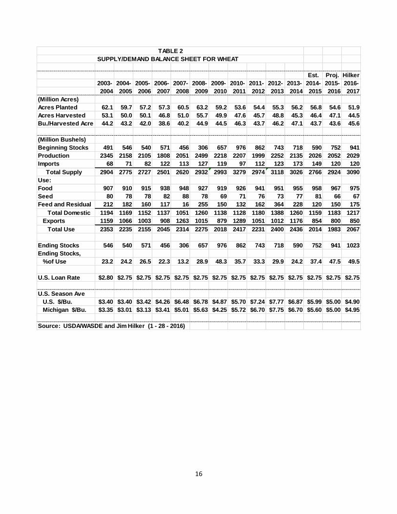
The 2015-16 U.S wheat marketing year is eight months in, and while we will discuss the projections, it appears the present projections will hold for the most part. The more interesting part is discussing the 2016-17 prospects. The wheat story is a bit like corn, ample supplies in the U.S. and the world.

2015-16

We planted 54.6 million acres of wheat for the 2015 wheat crop, down 2.2 million acres from 2014. Winter wheat accounted for 43.6 million of those acres, down 100,000 acres, spring wheat planted acres were up about 222,000 acres at 13.24 million acres, and durum wheat planted acres were up significantly at 1.94 million acres, up 432,000 acres, as they, unlike the Corn/Soybean Belt, didn’t have a wet spring like they had the previous two years.

Harvested acres came in at 47.1 million acres, up 700,000 acres. The all wheat yield was a below trend 43.6 bushels per acre. This put 2015 total wheat production at 2,052 million bushels, up only 27 million bushels from 2014. Michigan planted 510,000 acres of wheat for 2015, down 40,000 acres from 2014 and 110,000 from 2013, as we had late soybean harvests in 2013 and 2014. Michigan harvested 475,000 acres for grain. Michigan’s 2015 wheat yield was a record 81 bushels per acre, up 7 bushels per acre from 2014 and 5 bushels above the previous record set in 2012. Beginning stocks were a large 752 million bushels, up 162 million bushels from 2014-15. Total 2015-16 wheat supplies were 2,924 million bushels when 120 million bushels of imports and beginning stocks are added to production. This is up 5.7% from 2014-15. Domestic use of wheat in the U.S. for 2015-16 is projected to be up 24 million bushels from 2014-15 at 1,183 million bushels. Feed use is expected to be 150 million bushels as corn continued to be relatively cheaper. Exports are projected to be down 54 million bushels from last year at 800 million bushels. This is due to the rest of the world having a record wheat crops for the third year in a row. Projected 2015-16 U.S. ending stocks are 941 million bushels. This is 47.5% of use, up from last year’s 37.4% of use, way, way, more than adequate, in fact, very burdensome. The 2015-16 average weighted wheat price is expected to be $5.00 per bushel. Check out Table 2. 2016-17

The winter wheat seedings report showed 36.6 million acres of winter wheat planted for 2016, down sharply from 39.5 million acres last year and 42.4 million acres the year before. This decrease is mostly due to expected returns versus planting issues. I expect spring wheat plantings to be 13.3 million acres and durum wheat plantings to be 1.95 million acres, up a little from last year as a few marginal acres will be taken out of row crops. I expect total wheat planted acres to be 51.9 million acres for 2016-17 as shown in Table 2. I am projecting a normal percent harvested, which would put harvested acres at 44.5 million acres.

15

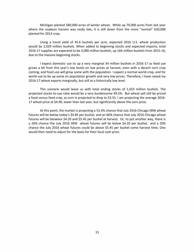
Michigan planted 580,000 acres of winter wheat. While up 70,000 acres from last year where the soybean harvest was really late, it is still down from the more “normal” 620,000 planted for 2013 crop.

Using a trend yield of 45.6 bushels per acre, expected 2016 U.S. wheat production would be 2,029 million bushels. When added to beginning stocks and expected imports, total 2016-17 supplies are expected to be 3,090 million bushels, up 166 million bushels from 2015-16, due to the massive beginning stocks.

I expect domestic use to up a very marginal 34 million bushels in 2016-17 as feed use grows a bit from this year’s low levels on low prices at harvest, even with a decent corn crop coming, and food use will grow some with the population. I expect a normal world crop, and for world use to be up some on population growth and very low prices. Therefore, I have raised my 2016-17 wheat exports marginally, but still at a historically low level.

This scenario would leave us with total ending stocks of 1,023 million bushels. The

projected stocks-to-use ratio would be a very burdensome 49.5%. But wheat will still be priced a food versus feed crop, as corn is projected to drop to $3.55. I am projecting the average 2016-17 wheat price at $4.90, lower than last year, but significantly above the corn price.

At this point, the market is projecting a 53.3% chance that July 2016 Chicago SRW wheat futures will be below today’s $4.85 per bushel, and an 60% chance that July 2016 Chicago wheat futures will be between $4.20 and $5.45 per bushel at harvest. Or, to put another way, there is a 20% chance the July 2016 SRW wheat futures will be below $4.20 per bushel, and a 20% chance the July 2016 wheat futures could be above $5.45 per bushel come harvest time. One would then need to adjust for the basis for their local cash price.

16

Est. Proj. Hilker

2003- 2004- 2005- 2006- 2007- 2008- 2009- 2010- 2011- 2012- 2013- 2014- 2015- 2016-

2004 2005 2006 2007 2008 2009 2010 2011 2012 2013 2014 2015 2016 2017

(Million Acres)

Acres Planted 62.1 59.7 57.2 57.3 60.5 63.2 59.2 53.6 54.4 55.3 56.2 56.8 54.6 51.9

Acres Harvested 53.1 50.0 50.1 46.8 51.0 55.7 49.9 47.6 45.7 48.8 45.3 46.4 47.1 44.5

Bu./Harvested Acre 44.2 43.2 42.0 38.6 40.2 44.9 44.5 46.3 43.7 46.2 47.1 43.7 43.6 45.6

(Million Bushels)

Beginning Stocks 491 546 540 571 456 306 657 976 862 743 718 590 752 941

Production 2345 2158 2105 1808 2051 2499 2218 2207 1999 2252 2135 2026 2052 2029

Imports 68 71 82 122 113 127 119 97 112 123 173 149 120 120

Total Supply 2904 2775 2727 2501 2620 2932 2993 3279 2974 3118 3026 2766 2924 3090

Use:

Food 907 910 915 938 948 927 919 926 941 951 955 958 967 975

Seed 80 78 78 82 88 78 69 71 76 73 77 81 66 67

Feed and Residual 212 182 160 117 16 255 150 132 162 364 228 120 150 175

Total Domestic 1194 1169 1152 1137 1051 1260 1138 1128 1180 1388 1260 1159 1183 1217

Exports 1159 1066 1003 908 1263 1015 879 1289 1051 1012 1176 854 800 850

Total Use 2353 2235 2155 2045 2314 2275 2018 2417 2231 2400 2436 2014 1983 2067

Ending Stocks 546 540 571 456 306 657 976 862 743 718 590 752 941 1023

Ending Stocks,

%of Use 23.2 24.2 26.5 22.3 13.2 28.9 48.3 35.7 33.3 29.9 24.2 37.4 47.5 49.5

U.S. Loan Rate $2.80 $2.75 $2.75 $2.75 $2.75 $2.75 $2.75 $2.75 $2.75 $2.75 $2.75 $2.75 $2.75 $2.75

U.S. Season Ave

U.S. $/Bu. $3.40 $3.40 $3.42 $4.26 $6.48 $6.78 $4.87 $5.70 $7.24 $7.77 $6.87 $5.99 $5.00 $4.90

Michigan $/Bu. $3.35 $3.01 $3.13 $3.41 $5.01 $5.63 $4.25 $5.72 $6.70 $7.75 $6.70 $5.60 $5.00 $4.95

Source: USDA/WASDE and Jim Hilker (1 - 28 - 2016)

TABLE 2

SUPPLY/DEMAND BALANCE SHEET FOR WHEAT

17

SOYBEANS

2015-16

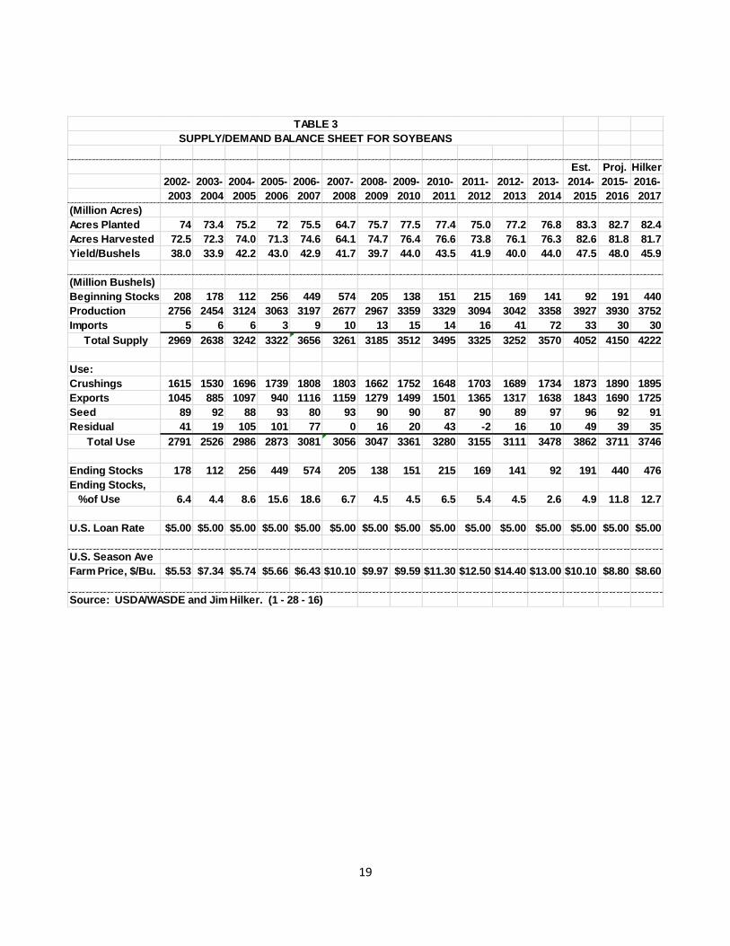
Soybean producers planted 82.7 million acres for 2015, down 600,000 acres from 2014, and 2.1 million acres below what producers intended to plant as of March 2015, largely due to the very wet spring and early summer. Harvested acres were 81.8 million acres. After the wet and late planting season, soybeans had a great growing season over most of the U.S. The 2015 U.S. soybean yield came in at record 48 bushels per acre, about two and a half bushels over trend and a half bushel higher than the record 2014 yield. This put soybean production for 2015 at a record 3,930 million bushels, but a mere 3 million bushel higher than the record 2014 production. Total supply for 2015-16 is 4,150 million when fairly low beginning stocks of 191 million bushels and imports were added to production, 100 million bushels greater than the record 2014-15 total supply.

Michigan planted 2.030 million acres of soybeans in 2015, and harvested 2.020 million

acres, both down 20,000 acres relative to 2014. Michigan’s 2015 soybean yield was a whopping 49 bushels per acre, up 6.5 bushel per acre from last year and 3 bushels above Michigan record of 46 set in 2006. This put 2015 Michigan soybean production at 99 million bushels, up 12 million bushels relative to 2014 due to the record yield.

U.S. 2015-16 total use is expected to be 3,711 million bushels, down 151 million bushels

from last year. While crush at 1,890 million bushels is expected to be up a bit, 17 million bushels, the increase was all in soy oil, up 2.5%, as soymeal production was down 0.7%. Soy oil exports and domestic use are projected to be up. On the soymeal side the small increase in domestic use will not come close to the decline in projected soymeal exports. Exports of whole soybeans are expected to be 1,690 million bushels, down 8.3% from the record exports 2014-15. Most of the exports and pretty much all the export sales will take place before the massive and perhaps record, very close to last year’s record, South American soybean crop harvest is completed. China continues to account for about 62% of both the world and U.S. exports.

This will put projected 2015-16 soybean ending stocks at a burdensome 440 million

bushels, 11.8% of projected use. Large world supplies will keep a lid soybean prices for the remainder of the marketing year if we have a normal 2016 soybean growing season. The projected U.S. 2015-16 average price is expected to be $8.80 after all is said and done.

2016-17

I expect 82.4 million acres to be planted to soybeans, only 300,000 acres less than last year. I expect some marginal land will be taken out of soybeans due to the low price. In fact, given the amount of prevented planting last year, this implies over a million marginal acres will be taken out of what would have been soybeans last year. There are several factors suggesting a relative shift from soybeans. Primarily returns per acre. In order to have a soybean price to give soybeans an equivalent returns per acre we will need relatively fewer acres this year. I project 2015 harvested acres to be a normal percentage of planted acres which would be 81.7 million acres. Using a trend yield of 45.9 bushels per acre, 2016 U.S. soybean production would be 3,752 million bushels, which would be a third largest crop on record after 2014 and 2015.

18

I expect crush to be up slightly as shown in Table 3 as we will be up in livestock numbers, but exports of oil and meal will likely be stagnant. However I expect soybean exports to be up a little despite another huge South American soybean crop this year, but with a normal South American soybean crop next year and decent world demand. Total U.S. disappearance is expected to be 3,746 million bushels, second largest on record. However, despite the large disappearance, projected 2016-17 ending stocks are projected to be 476 million bushels, 12.7% of use. I project the average U.S. 2016-17 soybean price will be $8.60.

At this point, the futures markets are expecting about this projected price. The market is

projecting a 52% chance that November 2016 soybean futures will be below today’s $8.90 per bushel, and a 60% chance that November 2016 soybean futures will be between $7.70 and $9.85 per bushel at harvest. Or, to put another way, there is a 20% chance the November 2016 soybean futures will be below $7.00 per bushel per bushel, and a 20% chance the November 2016 soybean futures could be above $9.85 per bushel come harvest time. Remember, you still need to subtract your basis from those numbers to get your local cash price.

19

Est. Proj. Hilker

2002- 2003- 2004- 2005- 2006- 2007- 2008- 2009- 2010- 2011- 2012- 2013- 2014- 2015- 2016-

2003 2004 2005 2006 2007 2008 2009 2010 2011 2012 2013 2014 2015 2016 2017

(Million Acres)

Acres Planted 74 73.4 75.2 72 75.5 64.7 75.7 77.5 77.4 75.0 77.2 76.8 83.3 82.7 82.4

Acres Harvested 72.5 72.3 74.0 71.3 74.6 64.1 74.7 76.4 76.6 73.8 76.1 76.3 82.6 81.8 81.7

Yield/Bushels 38.0 33.9 42.2 43.0 42.9 41.7 39.7 44.0 43.5 41.9 40.0 44.0 47.5 48.0 45.9

(Million Bushels)

Beginning Stocks 208 178 112 256 449 574 205 138 151 215 169 141 92 191 440

Production 2756 2454 3124 3063 3197 2677 2967 3359 3329 3094 3042 3358 3927 3930 3752

Imports 5 6 6 3 9 10 13 15 14 16 41 72 33 30 30

Total Supply 2969 2638 3242 3322 3656 3261 3185 3512 3495 3325 3252 3570 4052 4150 4222

Use:

Crushings 1615 1530 1696 1739 1808 1803 1662 1752 1648 1703 1689 1734 1873 1890 1895

Exports 1045 885 1097 940 1116 1159 1279 1499 1501 1365 1317 1638 1843 1690 1725

Seed 89 92 88 93 80 93 90 90 87 90 89 97 96 92 91

Residual 41 19 105 101 77 0 16 20 43 -2 16 10 49 39 35

Total Use 2791 2526 2986 2873 3081 3056 3047 3361 3280 3155 3111 3478 3862 3711 3746

Ending Stocks 178 112 256 449 574 205 138 151 215 169 141 92 191 440 476

Ending Stocks,

%of Use 6.4 4.4 8.6 15.6 18.6 6.7 4.5 4.5 6.5 5.4 4.5 2.6 4.9 11.8 12.7

U.S. Loan Rate $5.00 $5.00 $5.00 $5.00 $5.00 $5.00 $5.00 $5.00 $5.00 $5.00 $5.00 $5.00 $5.00 $5.00 $5.00

U.S. Season Ave

Farm Price, $/Bu. $5.53 $7.34 $5.74 $5.66 $6.43 $10.10 $9.97 $9.59 $11.30 $12.50 $14.40 $13.00 $10.10 $8.80 $8.60

Source: USDA/WASDE and Jim Hilker. (1 - 28 - 16)

SUPPLY/DEMAND BALANCE SHEET FOR SOYBEANS

TABLE 3

20

2016 ANNUAL LIVESTOCK OUTLOOK Jim Hilker Cattle

The numbers show that traditional feedlots made economic profits of -$304 per head in

2015, yes, negative, and did not have one profitable month. The annual loss was the biggest in our data set which go back into the 1970’s. After making economic profits the first 11 months of 2014, and expectations of high steer prices in 2015, feedlots bid up feeder prices early in the year. Then fed steer prices dropped as we went through the year, especially the last four months. With breakeven prices early in 2016 being nearly $160 per cwt. before dropping off to $147 per cwt. around April, does not make for a good start to this year. Huge losses relative to full cost should fall as we go through 2016, but it is hard to see a month with economic (full costs) profits at this point.

Cow calf returns on average were positive for a sixth year in a row in 2015. The difference is profits were more widespread the past two years due to less weather issues. In the first four years of average profits, many areas with drought had losses. In 2014 cow-calf returns over cash cost, including pasture rent, at $530.00 per cow, was the highest in our records going back into the 1970’s. And while dropping off to $301 per cow in 2015, it was still the second highest. At this point, we are looking for returns to be about $200 per head for 2016, still higher than any year going back past 1987.

January 1, 2016 Cattle Inventory Report for the second year in a row, after seven years of decline, showed an increase. The U.S. had 91.99 million head of cattle and calves as of January 1, 3.2% above 2014, but remember, 2013 was the smallest inventory since 1951. USDA estimated the total U.S. cow herd, including dairy, at 39.65 million head, up 2.7% from a year ago. Beef cows were reported at 30.331 million head, 3.5% larger than a year ago.

Beef cow replacements on January 1, 2016 were 6285.2 million, up a 3.3% over last

year. The number of beef cow replacement heifers expected to calve in 2015 at 3.925 million head was up 5.7% in 2015. USDA reported the 2015 calf crop at 34.3 million head, 2.3% larger than 2014. This should lead to a larger calf crop again in 2016.

As of January 1, the calculated available supply of feeder cattle outside feedlots was

25.913 million head, 5% more than 2015. Cattle on Feed in all feedlots January 1 were 13.18 million head, up 1.2% relative to last January 1.

All cattle and calves in Michigan on January 1, 2016, were at 1,150,000 head, up 30,000

head, up 2.7%. All cows that had calved were at 530,000 head, up 3.9%. Beef cows were up 10.3%, at 118,000. Dairy cows numbers were put at 412,000, up 2.2%. Beef cow replacements were up 4,000 head, 17.4%, at 27,000, while dairy cow replacements were up 5,000 head, 3%, at 167,000 head. Michigan’s 2015 calf crop was 400,000, 3.9%. The survey does not distinguish between beef and dairy calves. Michigan had 170,000 cattle on feed January 1, up 6.3% from last year.

The following estimates for cattle and hogs are made in conjunction with the Livestock

Marketing Information Center, which I belong to. It is a group supported by Universities to

21

provide efficiencies, i.e., less duplication of work by folks such as myself. U.S. commercial beef production is expected to be up 2.6% for 2016, as slaughter is expected to be up 2.1% with dressed weights being up 0.4%. Steer prices are expected to average in the $135-148 per cwt. for 2016, down 7.8%, after averaging $148.12 for 2015. The 700-800# feeder steers are expected to average $163-169 per cwt. in 2016, down from $208.21 for 2015, with 500-600# feeder calves averaging $196-203 per cwt., versus $251.25 in 2015.

In the first quarter of 2016, commercial beef production is expected to be up 2.3%.

Steer prices are expected to average $136-138 per cwt., with feeder steers averaging $164-168 per cwt., and feeder calves averaging $195-200 per cwt. In the second quarter, production is expected to be up 1.1%, with steer prices averaging $139-142 per cwt., feeder steers averaging $167-172 per cwt., and feeder calves averaging $198-205 per cwt.

In the third quarter, beef production is expected to be up 4.1%, with steer prices

averaging $133-137, feeder steers averaging $162-168, and feeder calves averaging $200-208. In the fourth quarter, beef production is expected to be up2.6%, with steer prices averaging $131-136, feeder prices averaging $159-166, and feeder calves averaging $191-200, all per cwt.

Hogs

Farrow-to-finish hog operations had a reasonably profitable 2015, profitable 8 of the 12 months, after a very profitable 2014. However, returns were negative the last two months of 2015 to the tune of $15 and $18’s per head. Returns may be mixed in 2016, likely struggling at the beginning and the end of the year.

All hogs and pigs on December 1, 2015 were up 1% from December 1, 2014. The

breeding herd was up 1.0% from the same period a year earlier. And market hogs on hand December 1 were also up 1.0% from 2014. The September-November pig crop was down 1% as fall farrowings were down 4%, and the pigs saved per litter were up 3%. This will be the bulk of the spring marketings. December- February farrowing intentions were down 2%, so if pigs saved per litter is up 1-2%, this indicates summer marketings will likely be about even. March-May farrowing intentions were even, so with the normal 1-2 % increase in pigs saved per litter, fall marketing will be up 1-2%.

The Michigan breeding herd stayed even at 110,000 head on December 1, 2015, the same as December 1, 2014, 2013, 2012, 2011, and 2010. We had 990,000 market hogs on hand, up 4% from last year. Sows farrowing in Michigan were down 6% this past fall, at 50,000. Pigs saved per litter were 10.7 versus 10.2 last fall. This put our total fall pig crop 99% versus the previous year at 535,000 head. Michigan’s Dec-Feb farrowing intentions are down 6% and the March-May farrowing intentions are down 2%.

Pork production is expected to be up 1.5% in 2016 versus 2015 as slaughter is expected to be up 1.3% with weights being up 0.1%. Carcass prices, National Weighted Average Base (multiply by .76 to have approximate live price projections) are expected to average in the $66-70 per cwt. range for all of 2016, down 2.9% relative to 2015.

In the first quarter of 2016, pork production is expected to be up 3.8%, with carcass

prices averaging $60-62 per cwt., down 11%. In the second quarter, production is expected to

22

be up 0.3%, with carcass prices averaging $73-76 per cwt., up 1.3%. In the third quarter, production is expected to be up 0.7%, with carcass prices averaging $73-77 per cwt., up 0.5%. In the fourth quarter, production is expected to be up 1.3%, with carcass prices averaging $59-64 per cwt., down 0.7%.

23

2016 DAIRY SITUATION AND OUTLOOK Christopher Wolf

Michigan milk production growth continued in 2015 finishing the year with a total of 10.2 billion pounds. This represented 6.5% growth over a year earlier. Since 2000, milk production growth has averaged 4%, almost equally split between growth in milk cows (2.1% annual growth rate) and growth in productivity (1.9% annual growth in milk per cow). 2015 was notable nationally because other major Northeast (i.e., New York) and Upper Midwest (i.e., Wisconsin and Minnesota) states also realized large milk production growth rates, while milk production in the Pacific and Southwest states declined. In particular, California milk production declined 3.4% in 2015. California feed prices have been significantly affected by the drought with corn and hay cash prices often 20% plus higher than Michigan prices. The real effect of these higher prices has shown up in milk per cow in California where the average cow produced about 900 pounds less in 2015 than the average Michigan milk cow.

Figure 1. Michigan milk production, cows and milk/cow, 2010-2015

One of the results of the milk production growth in and around Michigan were periodic shortages in processing capacity. For Michigan dairy farmers, these processing issues manifested themselves in relatively lower milk prices in some months. Figure 2 displays the Michigan mailbox milk price and the Class III milk price (milk for cheese production). The “basis” for farm milk price is the difference between these two prices. As the figure shows, we generally expect this basis to be a positive value. The Michigan basis averaged $1.20 per cwt. from 2010 through 2015. In previous years a negative basis indicated a large monthly increase in Class III prices and the mailbox price quickly followed—see 2012 as an example. In 2015, the summer months produced a negative Michigan milk price basis because of processing capacity issues. The basis

24

recovered in the fall months but with processing plants full in Wisconsin and other surrounding states, the basis issues are likely to remain for Michigan dairy farmers in 2016.

Figure 2. Michigan mailbox and Class III milk price

On the demand side, the U.S. market remains positive and growing. Consumption trends for many dairy products remain favorable with increased per capita consumption of cheese and Greek yogurt. The outlook for milk components as milk ingredients in other food and beverage products is also a positive for consumption. Domestic butter demand has also remained strong through and even past the holidays resulting in a US cash price that has been far above world price for a good part of the past year.

There are several on-going supply and demand issues currently affecting international dairy markets. With respect to supply, 2015 was a catastrophically poor profitability year in New Zealand resulting in a large decline in milk production in the second half of the year. In the European Union, the phase out of milk production quotas was recently completed. Without supply control, milk production in several countries took off. Notably the Netherlands (+7%) and Ireland +10%) had large milk production increases in 2015. This growth took place in the face of lower milk production prices. The Russian dairy product import embargo continues to weigh heavily over the milk market and contributed to the lower EU farm milk prices. China was also a relatively smaller purchaser international dairy demand in 2015 and questions about the continued growth of the Chinese economy driving world demand remain unanswered. For U.S. dairy exports, the result was a decline in value after strong growth in the previous five years (Figure 3). This decline in value reflected both a decline in the price of products exported as well as a decline in the quantity of some products. In particular, the aforementioned high domestic butter price resulted in uncompetitive US exports and a significant increase in butter imports.

25

Figure 3. Value of U.S. Dairy Exports

As of this writing, the futures market expects a recovery in milk prices in the second half

of 2016. The increase is anticipated to be about $2 per cwt. more than January prices for both Classes III and IV. This recovery appears to assume that the low farm milk prices in the EU and US will put the brakes on milk production growth. However, fundamentals remain bearish at the current time. While US cheese and milk powder prices are at or near international prices, US butter prices are holding at about a 50 percent premium to world butter prices. With current projected corn and soybean meal prices, the US income over feed cost margin for 2016 is projected to average $8.30 per cwt. which is close to the long-term average. This income over feed margin level would be neutral to milk production growth on the whole but of course there are regional issues. It is likely that milk production growth will continue in Michigan and surrounding Upper Midwest states and contract in the West and Southwest regions. Drought coupled with the severe winter weather in New Mexico and Texas are likely to plague milk production for months to come. On the whole average 2016 dairy farm returns are projected to be quite similar to 2015.

26

TAXES IN 2015 and 2016 Larry Borton and John Jones

Laws and rules changed many items in 2015 that will affect taxpayers in years to come. Let’s look at some of them that may affect farmers. Congress has made some changes which will ease tax planning for farmers. The Internal Revenue Service changed some rules which may help with capitalization and repair decisions. Other law changes allow increased penalties for neglecting information requirements. Some Social Security changes reduce options in retirement.

In December 2014, the direct expensing maximum limit was increased to $500,000 with a phase-out beginning at $2,000,000. However, the President would only sign that extenders bill for one year and this provision expired two weeks later at the end of 2014. We expected many expired provisions from that law to be extended again, and this finally occurred when the Protecting Americans from Tax Hikes (PATH) Act was passed and signed on December 18, 2015. These provisions included the $500,000 of direct expensing which is now permanent. Like before, the direct expensing phase-out still begins at $2,000,000 of qualified property placed in service. Direct expensing is for new or used depreciable property but some farm property is not eligible. For example, general purpose farm buildings, like a machinery shop are not eligible. The PATH Act also extends the 50% bonus depreciation, which does apply to almost any original use (new) farm property. The 50% applies for 2015-2017, then decreases to 40% in 2018, then 30% in 2019, then disappears.

Bonus cannot be used by fruit farmers who elected out of the uniform capitalization rules. Normally they would capitalize all the costs, including a portion of overhead costs like utilities and office expenses, until the trees, vines or bushes are in economic production. Electing out allows them to expense all costs except the cost of the actual plants. To offset this privilege they are required to use slower straight line depreciation (called ADS) on their entire farm’s depreciable property and are not allowed to use the bonus provision. The rule will preclude most Michigan fruit farmers from using the provision in the new law that allows bonus depreciation on the cost of trees or vines when planted or grafted. Most Michigan fruit farmers will continue using ADS for depreciation, subtract most costs when paid while bringing new blocks or areas into production, and then direct expense the cost of the plants the year that economic production begins.

The repair and capitalization regulations from a couple years ago tried to simplify the decision process for determining whether to call something a repair and expense it or capitalize and depreciate it. If an expenditure is for restoration, betterment, or adaptation to a new use, then it should be capitalized.

The IRS announced a new rule in November. Unless a farm has an AFS (Applicable Financial Statement), and very few in Michigan would have this, the taxpayer may deduct the cost of any item or unit of property that is not above an elected amount. The maximum amount increased to $2,500 (formerly $500) but a smaller amount may be elected. Now any item of tangible personal property (tool, pallet fruit box, dairy or breeding animal, piece of equipment) up to that elected amount must be deducted and not capitalized for depreciation. When that

27

item is sold or culled, then the income gets reported on Schedule F which makes it subject to self-employment taxes.

Within these capitalization regulations, the prepaid expensing rules for cash accounting farmers really have not changed. The expenditure counts as a deduction when paid. To substantiate the expense, the invoice should show quantities and products. Depositing money with the vendor without showing quantities and products is not a prepaid expense. Also, it must be for a business purpose, like assuring a supply or getting a discount for early payment. Saving on taxes is not considered a business purpose by the IRS. Another change for 2016 changed penalties for not filing information returns. They increased due to the Tax Prevention Act of 2014 and apply to any information return or statement due after December 31, 2015. Up to 30 days late increased from $30 to $50. After 30 days the penalty becomes $60, then $100 and finally $250 for intentional disregard. This penalty would apply to both the return that must be filed with the IRS and the copy that must be sent to the payee. Form 1099 would come under this rule. A 1099 may be required when renting property between entities even though all are in the same family. If a retired farmer rents land to his son, the son should give a Form 1099 to dad and the IRS. Also, payments to veterinarians require a Form 1099, because the law counts them as medical services. The IRS matches these Form 1099s to the recipient’s tax return. Some Social Security benefit strategies will disappear in 2016. The file and suspend method of an individual filing for benefits and allowing the spouse to obtain spousal benefits ceases in May 2016. Under previous rules, the individual would suspend benefits and quit receiving payments while the spouse continued getting benefits. This would allow both to continue growing their future monthly benefit amount up to age 70, while the household still received benefits. Anyone born on or before May 1, 1950 may still use this if paperwork is done by April 29, 2016. Another previous strategy for a dual-earner couple is the spousal benefit method, which disappears for those born after January 1, 1954. After reaching full retirement age (66 years old if born in 1954 or before), a spouse can choose to receive only spousal benefits while letting their own future monthly benefit increase until age 70. This allows them to switch to their own benefit if it is higher than the spousal benefit. When someone applies for benefits without these two methods, the Social Security Administration will just take the highest amount based either on a person’s earnings or as a spouse. Social Security retirement benefits continue to be based on the highest 35 years of earnings and the law allows someone to get credits toward retirement benefits even with low net income. If a farmer has a tough year with little self-employment earnings, using the farm optional method will cost about $700 in self-employment tax, but gets them one year (or four quarters) towards the 35 years. Filing for the Earned Income Credit may get half or more of this back. This permits an inexpensive way to get Social Security credits.

Health insurance questions related to Obamacare continued in 2015 and will continue in 2016. The penalties for not having health insurance keep increasing as part of the individual shared responsibility. For employers, with more than one employee (which is most Michigan farms), the penalty for assisting employees with health insurance is $100 per employee per day if the insurance does not meet all the market reforms.

28

Many other tax changes occurred in 2015 including making the American Opportunity Credit for college students permanent, as well as the $250 deduction for teachers who have classroom expenses or professional development costs. Also, contributions of real property for conservation purposes can be at a higher level which may affect donations of development rights. Another provision of the new law which is now permanent, is the option to take an itemized deduction for sales taxes rather than state income taxes. This is especially useful in Florida or Texas with no state income taxes but might be used in Michigan when a personal vehicle is purchased and the sales tax for a year is more than the state income taxes. These items represent changes which commonly affect farmers in Michigan. Please keep your income tax preparer in the loop when considering actions that would affect your income taxes. Planning ahead helps prevent paying more than the law requires. Finally, we need to emphasize that Identity theft continues to plague taxpayers. We have seen this show up when a thief files as the taxpayer and gets a refund before the taxpayer files. Filing early helps reduce the chances of this occurring. Most of us have probably received calls telling us that we owe money to the IRS. This “phishing” is rampant. Last week a student walked into our office on the cell phone with an alleged IRS employee on the line threatening to arrest the student if they did not immediately pay the “federal student tax.” However, no such tax exists. Page 98 of the 2015 Farmer’s Tax Guide points out items that the IRS will NEVER do including:

Call to demand immediate payment, nor will the agency call about taxes without first having mailed you a bill.

Ask for credit or debit card numbers over the phone.

Threaten to bring in local police or other law enforcement groups to have you arrested for not paying.

The caller used all these tactics and the student hung up the phone. The student

received three more calls within the next five minutes but knew they were not legitimate calls. Another approach has been a call claiming to be from the IRS and needing personal and financial information in order to send you a refund. This is still phishing and is a scam!

29

FARM INCOME David B. Schweikhardt

Following a decade of strong farm income performance (and an all-time record performance in 2013), net farm income decreased by 38% in 2015, the largest single-year decrease since 1983. This decrease resulted from a decrease in revenues for most crop categories and virtually all livestock categories. Total farm production expenses witnessed a small decrease during 2015, but far less than the decrease in revenue. This outlook sets the stage for a highly uncertain outlook for 2016.

During the past decade, variations in income across the farm sector have been

especially pronounced, with the crop income outlook varying widely from the livestock income outlook. That trend is likely to continue in 2016, but with sharply different outlooks for the two industries than in recent years. In particular, the outlook for continued lower crop prices is likely to be the dominant factor in determining the income outlook in both the crop and livestock sectors in 2015.

2015 Farm Income Summary

Net farm income in the U.S. is estimated to have been $56 billion in 2015, compared to $90 billion in 2014 and a record $123 billion in 2013. This decrease resulted from a major decrease in total farm revenue ($43 billion), an increase in government payments (+$1.0 billion) and a decrease in expenses (-$14 billion). As a result of these changes, the 2015 level of net farm income fell below the 10-year average of $86 billion. The value of crop production in 2015 ($186 billion) decreased from $204 billion in 2013 due to decreases in revenues for most crop categories – feed grains (-$9 billion), food grains (-$4 billion), oilseeds (-$5 billion) all experienced decreases due to lower crop prices. Revenue for fruit and nut crops remained unchanged at $30 billion, while vegetables and melons (+$500 million) all experienced an increase in revenue.

At the same time, the value of livestock production decreased by $23.5 billion to a total

of $191 billion in 2015 on the basis of decreases in dairy production (-$24 billion) and meat animal production (-$10.7 billion), and poultry and egg revenue (+$1.1 billion).

Changes in production expenses continued to reflect the changing economic conditions

across production sectors in agriculture witnessed in recent years. In recent years, the farm income outlook across agricultural sectors (crop versus livestock sectors) has reflected widely divergent outlooks that resulted as high crop prices were reflected in increased feed expenses for livestock producers. In 2015, this situation continued its recent reversal as lower crop prices were reflected in a decrease in purchased feed costs for livestock producers (from $63 billion in 2014 to $58 billion in 2015). At the same time, livestock and poultry purchases were constant at $30.7 billion in 2015.

The decrease in revenue for crop production was partially offset by decreases or a

constant level of production costs for several expense categories. Seed ($30.7 billion) and electricity ($5.9 billion) expenses remained unchanged in 2015, while fertilizer (-$2.2. billion), pesticides (-$770 million), fuels (-$5.1 billion) and marketing, storage and transportation (-$200 million) decreased in 2015. Labor (+$1.6 billion), interest (+$3.2 billion), and repair and

30

maintenance (+$300 million) expenses increased in 2015. Rental payments to non-operator landlords decreased by $100 million in 2015 to $18.3 billion. This represented a decrease of $1.7 billion from the record highest level of rental payments in 2013. 2016 Farm Income Summary

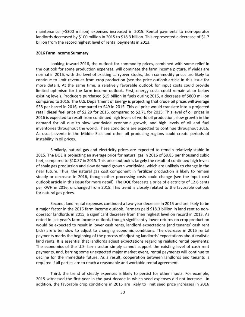
Looking toward 2016, the outlook for commodity prices, combined with some relief in the outlook for some production expenses, will dominate the farm income picture. If yields are normal in 2016, with the level of existing carryover stocks, then commodity prices are likely to continue to limit revenues from crop production (see the price outlook article in this issue for more detail). At the same time, a relatively favorable outlook for input costs could provide limited optimism for the farm income outlook. First, energy costs could remain at or below existing levels. Producers purchased $15 billion in fuels during 2015, a decrease of $800 million compared to 2015. The U.S. Department of Energy is projecting that crude oil prices will average $38 per barrel in 2016, compared to $49 in 2015. This oil price would translate into a projected retail diesel fuel price of $2.29 for 2016, compared to $2.71 for 2015. This level of oil prices in 2016 is expected to result from continued high levels of world oil production, slow growth in the demand for oil due to slow worldwide economic growth, and high levels of oil and fuel inventories throughout the world. These conditions are expected to continue throughout 2016. As usual, events in the Middle East and other oil producing regions could create periods of instability in oil prices.

Similarly, natural gas and electricity prices are expected to remain relatively stable in

2015. The DOE is projecting an average price for natural gas in 2016 of $9.85 per thousand cubic feet, compared to $10.37 in 2015. This price outlook is largely the result of continued high levels of shale gas production and slow demand growth worldwide, which are unlikely to change in the near future. Thus, the natural gas cost component in fertilizer production is likely to remain steady or decrease in 2016, though other processing costs could change (see the input cost outlook article in this issue for more detail). The DOE forecasts a price of electricity of 12.6 cents per KWH in 2016, unchanged from 2015. This trend is closely related to the favorable outlook for natural gas prices.

Second, land rental expenses continued a two-year decrease in 2015 and are likely to be

a major factor in the 2016 farm income outlook. Farmers paid $18.3 billion in land rent to non-operator landlords in 2015, a significant decrease from their highest level on record in 2013. As noted in last year’s farm income outlook, though significantly lower returns on crop production would be expected to result in lower cash rents, landlord expectations (and tenants’ cash rent bids) are often slow to adjust to changing economic conditions. The decrease in 2015 rental payments marks the beginning of the process of adjusting landlords’ expectations about realistic land rents. It is essential that landlords adjust expectations regarding realistic rental payments: The economics of the U.S. farm sector simply cannot support the existing level of cash rent payments, and, barring some unexpected major market event, rental payments will continue to decline for the immediate future. As a result, cooperation between landlords and tenants is required if all parties are to reach a reasonable and workable rental agreement.

Third, the trend of steady expenses is likely to persist for other inputs. For example, 2015 witnessed the first year in the past decade in which seed expenses did not increase. In addition, the favorable crop conditions in 2015 are likely to limit seed price increases in 2016

31

(see the input cost outlook article in this issue for more detail). Labor costs are likely to see an increase again in 2016.

Finally, the outlook for interest rates on production and asset loans is likely to remain

unchanged in 2016. In December 2015, the Federal Reserve raised the Federal Funds rate (bank lending rate) by one-quarter point to one-half percent. Other comments by the members of the Federal Reserve Open Market Committee (FOMC) suggested that three addition ¼ point increases would occur by the end of 2016. In making this decision, the FOMC members emphasized that labor market conditions had improved since the early part of the year and that inflation remained well within its stated target range of 2%.

At the same time, the FOMC statement emphasized that any future decisions about

interest rate increases would depend upon the status of economic conditions, including international conditions, later in 2016. At it’s January 2016 meeting, the FOMC reiterated that position.

Since the December FOMC announcement of a rate increase, economic conditions, particularly international conditions, have continued to change in a manner that has called into question the FOMC’s intentions of additional rate hike in 2016. In particular, continued slow economic growth and high unemployment in many countries has led those countries to adopt policies in conflict with U.S. monetary policy. While the Federal Reserve has increased its bank lending rate, the central banks of several other nations have indicated their intention to move in an opposite direction by reducing rates (or have already done so). Interest rates on government bonds of several European countries are now in negative territory (the bond buyer will receive less than the amount lent when the bond matures). Since the FOMC’s December decision to increase its Federal Funds rate, Japan has moved to reduce interest rates into negative territory, and Canada’s central bank officials have indicated a willingness to do so in the near future.

In each case, the move of the central bank in lowering interest rates into negative

territory has been an effort to stimulate its domestic economy by encouraging a depreciation of its currency exchange rates and increasing its exports. This flip side of this policy, of course, is that the widening gap between U.S. and foreign monetary policy will continue to strengthen the U.S. dollar and threatens to erode U.S. exports and increase U.S. imports. Such a policy of “exporting unemployment” via currency manipulation is likely to be a major obstacle to the Fed’s intention of increasing interest rates later this year. Indeed, interest rates on U.S. government bonds have fallen since the Fed’s December announcement, probably due in part to foreign bond buyers demanding U.S. bonds because of the extremely low returns available in other countries. Finally, additional pressure strengthening the U.S. dollar would increase the price of U.S. farm exports for foreign buyers, and would be an additional factor that is likely to limit improvements in U.S. crop and livestock prices in 2016. As noted last year in this article, though the outlook for interest rates is likely to be stable for the coming year, lenders are likely to continue using increased scrutiny of borrowers’ creditworthiness, with a particular emphasis on the farm’s liquidity status.