STACK MODELLING FOR TRANSPACIFIC REFINERS, RUTHERFORD

A PEL Company

STACK MODELLING FOR TRANSPACIFIC

REFINERS, RUTHERFORD

Transpacific Refiners

Job No: 6963

6 August 2012

6963 TPR stack modelling R3 Final ii

Transpacific Refiners | PAEHolmes Job 6963

PROJECT TITLE: Stack Modelling for Transpacific Refiners,

Rutherford

JOB NUMBER: 6963

PREPARED FOR: Nicholas Welbourne

Transpacific Refiners

PREPARED BY: Khalia Hill

DISCLAIMER & COPYRIGHT: This report is subject to the copyright

statement located at www.paeholmes.com ©

Queensland Environment Pty Ltd trading as

PAEHolmes ABN 86 127 101 642

DOCUMENT CONTROL

VERSION DATE PREPARED BY REVIEWED BY

D1 06.07.12 Khalia Hill J. Barnett

D2 11.07.12 Khalia Hill

D3 06.08.12 Khalia Hill J. Barnett

Queensland Environment Pty Ltd trading as

PAEHolmes ABN 86 127 101 642

SYDNEY:

Suite 203, Level 2, Building D, 240 Beecroft Road

Epping NSW 2121

Ph: +61 2 9870 0900

Fax: +61 2 9870 0999

BRISBANE:

Level 1, La Melba, 59 Melbourne Street, South Brisbane QLD 4101

PO Box 3306, South Brisbane QLD 4101

Ph: +61 7 3004 6400

Fax: +61 7 3844 5858

ADELAIDE:

35 Edward Street, Norwood SA 5067

PO Box 1230,Littlehampton SA 5250

Ph: +61 8 8332 0960

Fax: +61 7 3844 5858

PERTH:

Level 18, Central Park Building,

152-158 St Georges Terrace, Perth WA 6000

Ph: +61 8 9288 4522

Fax: +61 8 9288 4400

MELBOURNE:

Suite 62, 63 Turner Street, Port Melbourne VIC 3207

PO Box 23293, Docklands VIC 8012

Ph: +61 3 9681 8551

Fax: +61 3 9681 3408

GLADSTONE:

Suite 2, 36 Herbert Street, Gladstone QLD 4680

Ph: +61 7 4972 7313

Fax: +61 7 3844 5858

Email: [email protected]

Website: www.paeholmes.com

http://www.paeholmes.com/

mailto:[email protected]

http://www.paeholmes.com/

6963 TPR stack modelling R3 Final

TPR | PAEHolmes Job 6963

ES1 EXECUTIVE SUMMARY

Transpacific Refiners (TPR) are investigating potential effects on ground level concentration due to

changes in the stack parameters of the gas fired heater at their Rutherford refinery. Six scenarios

have been modelled to incorporate all combinations of two stack heights and three exit velocities.

Dispersion modelling conducted for this assessment has been based on a modelling system using

TAPM, CALMET and CALPUFF.

Initial modelling was carried out for 23 receptors in the area, which included the existing exit

velocity and the two stack heights (16 m and 25 m). Further modelling was then done for five on

site receptors for each of the six scenarios.

The results indicate that the largest reductions in ground level concentrations come from increasing

the stack height rather than the exit velocity. The most significant of these is in the H2SO4

concentrations (up to 45% by increasing to 25 m alone, and 46% for increasing stack height and

exit velocity).

6963 TPR stack modelling R3 Final 1


1 INTRODUCTION

Transpacific Refiners (TPR) operate an oil refinery that processes recycled oil feedstock, located

within an industrial area in Kyle Street, Rutherford. TPR wish to investigate the effects of increasing

the height of the Fired Heater stack on ground level concentrations in the area.

PAEHolmes has been commissioned to conduct dispersion modelling to assess the potential impact

of two different stack heights for the gas fired heater. The methodologies and results from this

modelling are presented in the following.

2 IMPACT ASSESSMENT CRITERIA

The New South Wales Environment Protection Authority (EPA) provides guidance for the selection

and configuration of air dispersion models, methodologies to be used to compile meteorological

datasets and emissions data, and specifies the assessment criteria to be used to evaluate

compliance. This guidance is the ‘Approved Methods for modelling and assessment of air pollutants

in New South Wales’ (DEC, 2005). The criteria are health-based and are consistent with the

National Environment Protection Measure for Ambient Air Quality (referred to as the Ambient Air-

NEPM) (NEPC, 1998).

Table 1 summarises the adopted air quality criteria for the six key air quality indicators that are

relevant to the scope of this study. Note that Benzene has been chosen for modelling as it

represents the highest proportion of total VOCs measured onsite and it has the most stringent

assessment criteria.

Table 1 Ambient Air Quality Criteria relevant to the Current Study (Source: Air NEPM)

Pollutant Averaging Period Maximum Concentration

µg/m3

PM10 24 hour 50

Annual 30

Benzene (VOCs) 1 hour 0.029

SO2

1 hour 570

24 hour 228

Annual 60

NO2 1 hour 246

Annual 62

H2SO4 mist (sulphuric acid) 1 hour 0.018

H2S Nose response time average

(99th Percentile) 3.45

Hydrogen Sulfide (H2S) is an odorous air pollutant and is reported as a peak concentration at an

approximately 1 second average. Therefore the 1 hour average ground level concentrations of H2S

are scaled with an appropriate peak-to-mean ratio from Table 2, which was a near field wake-

affected point for all atmospheric stability classes A to F.



Table 2 Factors for estimating peak concentrations in flat terrain (Source: Approved Methods)

Source Type Pasquil-Gifford stability class Near field P/M60*

Far field P/M60*

Area A, B, C, D 2.5 2.3

E, F 2.3 1.9

Line A-F 6 6

Surface wake-free point A, B, C 12 4

D, E, F 25 7

Tall wake-free point A, B, C 17 3

D, E, F 35 6

Wake-affected point A-F 2.3 2.3

Volume A-F 2.3 2.3 *Ratio of peak 1-second average concentrations to mean 1-hour average concentrations

3 DISPERSION MODELLING

The modelling has been carried out in general accordance with the ‘Approved Methods’ which specify

how assessments based on the use of air dispersion models should be undertaken.

Dispersion modelling conducted for this assessment has been based on a modelling system using

TAPM, CALMET and CALPUFF.

TAPM is a prognostic meteorological model that generates gridded three-dimensional meteorological

data for each hour of the model run period. CALMET, the meteorological pre-processor for the

dispersion model CALPUFF, calculates three-dimensional meteorological data based upon observed

ground and upper level meteorological data, as well as modelled data generated for example by

TAPM. CALPUFF then calculates the dispersion of plumes within this three-dimensional

meteorological field.

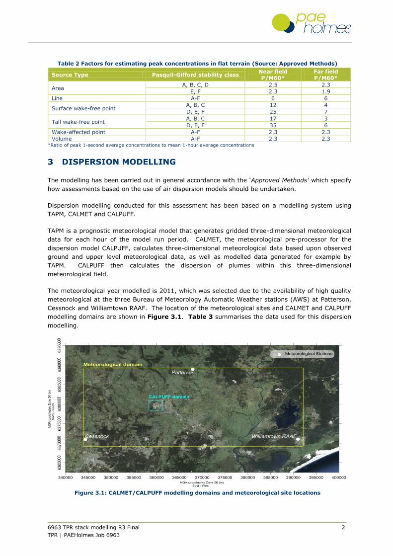
The meteorological year modelled is 2011, which was selected due to the availability of high quality

meteorological at the three Bureau of Meteorology Automatic Weather stations (AWS) at Patterson,

Cessnock and Williamtown RAAF. The location of the meteorological sites and CALMET and CALPUFF

modelling domains are shown in Figure 3.1. Table 3 summarises the data used for this dispersion

modelling.

Figure 3.1: CALMET/CALPUFF modelling domains and meteorological site locations



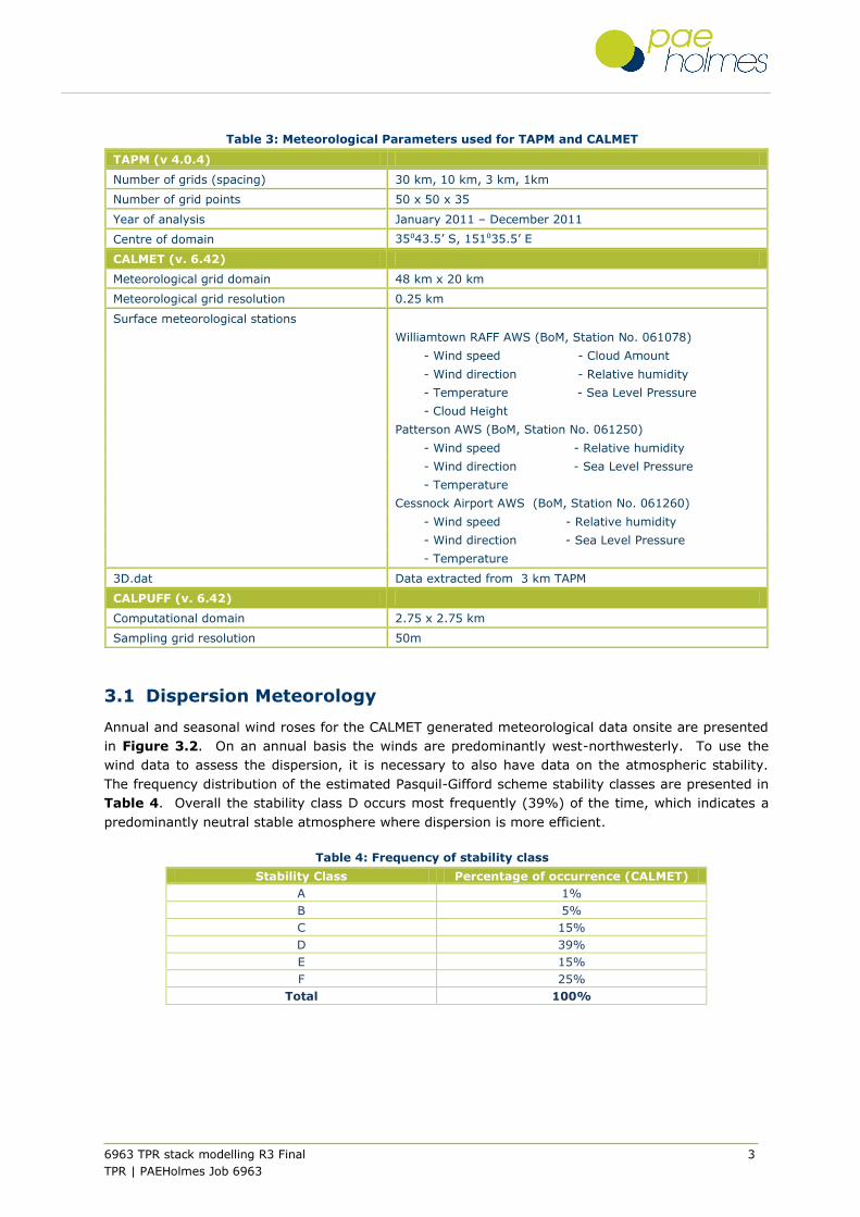
Table 3: Meteorological Parameters used for TAPM and CALMET

TAPM (v 4.0.4)

Number of grids (spacing) 30 km, 10 km, 3 km, 1km

Number of grid points 50 x 50 x 35

Year of analysis January 2011 – December 2011

Centre of domain 35⁰43.5’ S, 151⁰35.5’ E

CALMET (v. 6.42)

Meteorological grid domain 48 km x 20 km

Meteorological grid resolution 0.25 km

Surface meteorological stations

Williamtown RAFF AWS (BoM, Station No. 061078)

- Wind speed - Cloud Amount

- Wind direction - Relative humidity

- Temperature - Sea Level Pressure

- Cloud Height

Patterson AWS (BoM, Station No. 061250)

- Wind speed - Relative humidity

- Wind direction - Sea Level Pressure

- Temperature

Cessnock Airport AWS (BoM, Station No. 061260)

- Wind speed - Relative humidity

- Wind direction - Sea Level Pressure

- Temperature

3D.dat Data extracted from 3 km TAPM

CALPUFF (v. 6.42)

Computational domain 2.75 x 2.75 km

Sampling grid resolution 50m

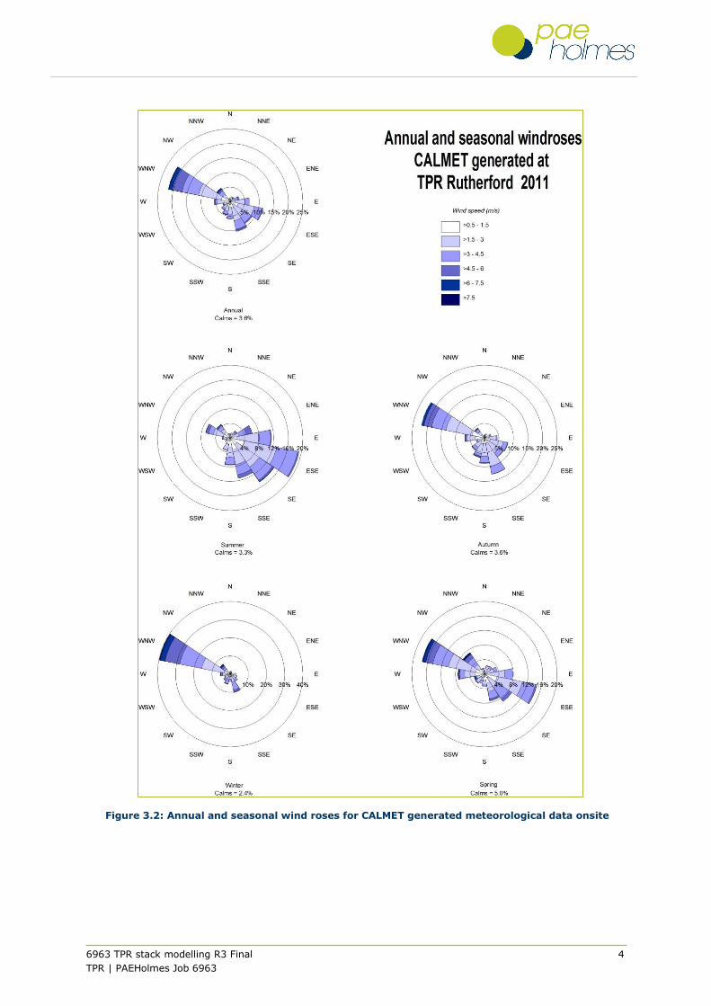
3.1 Dispersion Meteorology

Annual and seasonal wind roses for the CALMET generated meteorological data onsite are presented

in Figure 3.2. On an annual basis the winds are predominantly west-northwesterly. To use the

wind data to assess the dispersion, it is necessary to also have data on the atmospheric stability.

The frequency distribution of the estimated Pasquil-Gifford scheme stability classes are presented in

Table 4. Overall the stability class D occurs most frequently (39%) of the time, which indicates a

predominantly neutral stable atmosphere where dispersion is more efficient.

Table 4: Frequency of stability class

Stability Class Percentage of occurrence (CALMET)

A 1%

B 5%

C 15%

D 39%

E 15%

F 25%

Total 100%



Figure 3.2: Annual and seasonal wind roses for CALMET generated meteorological data onsite



4 EMISSION ESTIMATES

New Environment Quality (newEQ) has conducted regular stack testing at the Rutherford refinery for

each of the sources listed below:

Points 2 and 3 - 0.2 and 3.0 MW gas fired boilers

Point 5 - Light Ends Scrubber

Point 19 - stack that serves two gas fired heaters

o The thermal oil heater operates on natural gas and exhausts directly out of Point 19

(via in-duct monitoring point 18)

o The Fired Heater operates on natural gas and fuel gas from the process, and

exhausts to a SOX scrubber to control potential sulphur emissions. After passing

though the scrubber, emissions from the Fired Heater exhaust to point 19 (via in-

duct monitoring point 1)

Point 20 - exhaust emissions associated with operation of the reformer.

The point source locations are shown in Figure 4.1. Note that the point 4 flare stack is not subject

to testing in this assessment.

Figure 4.1: Source locations



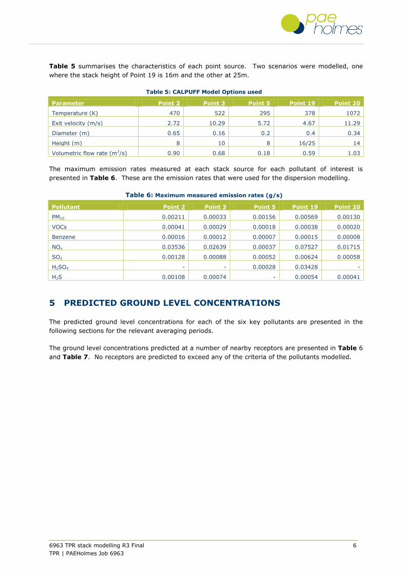
Table 5 summarises the characteristics of each point source. Two scenarios were modelled, one

where the stack height of Point 19 is 16m and the other at 25m.

Table 5: CALPUFF Model Options used

Parameter Point 2 Point 3 Point 5 Point 19 Point 20

Temperature (K) 470 522 295 378 1072

Exit velocity (m/s) 2.72 10.29 5.72 4.67 11.29

Diameter (m) 0.65 0.16 0.2 0.4 0.34

Height (m) 8 10 8 16/25 14

Volumetric flow rate (m3/s) 0.90 0.68 0.18 0.59 1.03

The maximum emission rates measured at each stack source for each pollutant of interest is

presented in Table 6. These are the emission rates that were used for the dispersion modelling.

Table 6: Maximum measured emission rates (g/s)

Pollutant Point 2 Point 3 Point 5 Point 19 Point 20

PM10 0.00211 0.00033 0.00156 0.00569 0.00130

VOCs 0.00041 0.00029 0.00018 0.00038 0.00020

Benzene 0.00016 0.00012 0.00007 0.00015 0.00008

NOx 0.03536 0.02639 0.00037 0.07527 0.01715

SO2 0.00128 0.00088 0.00052 0.00624 0.00058

H2SO4 - - 0.00028 0.03428 -

H2S 0.00108 0.00074 - 0.00054 0.00041

5 PREDICTED GROUND LEVEL CONCENTRATIONS

The predicted ground level concentrations for each of the six key pollutants are presented in the

following sections for the relevant averaging periods.

The ground level concentrations predicted at a number of nearby receptors are presented in Table 6

and Table 7. No receptors are predicted to exceed any of the criteria of the pollutants modelled.



Table 7: Predicted ground level concentrations at nearby residences for the 16m Point 19 stack

Table 8: Predicted ground level concentrations at nearby residences for the 25 Point 19 stack

Easting Northing H2S H2SO4 (SO3) SO2 VOCs PM10 NOx Benzene

99th

percentile

1 hour 1 hour 24 hour Annual 1 hour 24 hour Annual 1 hour Annual 1 hour

3.45 0.018 570 228 60 - 50 30 246 62 0.029

µg/m3 mg/m3 µg/m3 µg/m3 µg/m3 mg/m3 µg/m3 µg/m3 µg/m3 µg/m3 mg/m3

1 359332 6379827 1.20 0.0090 2.5 0.94 0.104 0.00039 1.16 0.13 38 1.61 0.00061

2 359810 6380106 0.12 0.0014 0.4 0.09 0.006 0.00006 0.10 0.01 6 0.10 0.00008

3 360241 6379147 0.09 0.0008 0.2 0.07 0.009 0.00003 0.08 0.01 3 0.15 0.00005

4 360134 6378983 0.07 0.0007 0.2 0.05 0.005 0.00003 0.06 0.01 3 0.08 0.00004

5 360115 6378743 0.03 0.0005 0.1 0.02 0.002 0.00002 0.03 0.00 2 0.03 0.00003

6 359822 6378743 0.02 0.0006 0.2 0.02 0.001 0.00003 0.03 0.00 3 0.02 0.00004

7 359608 6378819 0.02 0.0008 0.2 0.02 0.001 0.00003 0.03 0.00 3 0.02 0.00004

8 359814 6380102 0.12 0.0014 0.4 0.08 0.006 0.00006 0.09 0.01 6 0.10 0.00008

9 359285 6380087 0.37 0.0031 0.8 0.37 0.037 0.00013 0.41 0.04 13 0.58 0.00019

10 359266 6379626 0.31 0.0038 1.1 0.26 0.015 0.00018 0.32 0.02 17 0.24 0.00031

11 359372 6379611 0.28 0.0040 1.0 0.20 0.027 0.00016 0.25 0.03 16 0.43 0.00023

12 359441 6379596 0.26 0.0029 0.7 0.21 0.035 0.00011 0.25 0.04 11 0.57 0.00017

13 359479 6379592 0.27 0.0025 0.7 0.23 0.039 0.00010 0.26 0.05 10 0.62 0.00015

14 359536 6379588 0.27 0.0022 0.6 0.21 0.041 0.00009 0.25 0.05 9 0.66 0.00013

15 359631 6379615 0.28 0.0020 0.6 0.21 0.045 0.00010 0.25 0.05 10 0.72 0.00016

16 359734 6379741 0.23 0.0019 0.5 0.18 0.026 0.00009 0.20 0.03 8 0.40 0.00014

17 359696 6379908 0.19 0.0021 0.5 0.14 0.012 0.00008 0.15 0.01 8 0.19 0.00012

18 359624 6379939 0.21 0.0023 0.6 0.15 0.014 0.00009 0.16 0.02 9 0.22 0.00013

19 359475 6379939 0.37 0.0038 1.0 0.38 0.028 0.00015 0.42 0.03 15 0.42 0.00023

20 359281 6379969 0.75 0.0061 1.6 0.80 0.086 0.00024 0.88 0.10 25 1.34 0.00035

21 359239 6379874 1.29 0.0084 2.1 1.63 0.261 0.00039 1.85 0.30 34 4.01 0.00056

22 359186 6379733 0.89 0.0092 2.5 0.80 0.065 0.00040 0.92 0.08 40 1.01 0.00058

23 359171 6379642 0.35 0.0049 1.3 0.34 0.019 0.00020 0.39 0.02 20 0.30 0.00033

Criteria

Units

Receptor

ID

Easting Northing H2S H2SO4 (SO3) SO2 VOCs PM10 NOx Benzene

99th

percentile

1 hour 1 hour 24 hour Annual 1 hour 24 hour Annual 1 hour Annual 1 hour

3.45 0.018 570 228 60 - 50 30 246 62 0.029

µg/m3 mg/m3 µg/m3 µg/m3 µg/m3 mg/m3 µg/m3 µg/m3 µg/m3 µg/m3 mg/m3

1 359332 6379827 0.97 0.0064 1.7 0.39 0.053 0.00033 0.68 0.08 27 1.00 0.00058

2 359810 6380106 0.10 0.0008 0.2 0.05 0.004 0.00005 0.05 0.01 4 0.07 0.00008

3 360241 6379147 0.09 0.0006 0.2 0.06 0.009 0.00003 0.07 0.01 3 0.15 0.00004

4 360134 6378983 0.07 0.0006 0.2 0.05 0.005 0.00003 0.06 0.01 3 0.08 0.00004

5 360115 6378743 0.03 0.0005 0.1 0.03 0.002 0.00002 0.03 0.00 2 0.03 0.00003

6 359822 6378743 0.02 0.0006 0.2 0.03 0.001 0.00003 0.03 0.00 3 0.02 0.00004

7 359608 6378819 0.02 0.0007 0.2 0.03 0.001 0.00003 0.03 0.00 3 0.02 0.00004

8 359814 6380102 0.10 0.0008 0.2 0.05 0.004 0.00005 0.05 0.01 4 0.07 0.00008

9 359285 6380087 0.35 0.0024 0.7 0.26 0.028 0.00011 0.31 0.03 11 0.47 0.00018

10 359266 6379626 0.30 0.0028 0.9 0.21 0.013 0.00016 0.27 0.02 14 0.21 0.00031

11 359372 6379611 0.27 0.0026 0.7 0.17 0.020 0.00012 0.22 0.03 11 0.35 0.00022

12 359441 6379596 0.25 0.0023 0.6 0.16 0.026 0.00009 0.20 0.03 9 0.45 0.00016

13 359479 6379592 0.24 0.0021 0.6 0.16 0.030 0.00008 0.20 0.04 9 0.52 0.00014

14 359536 6379588 0.24 0.0018 0.5 0.20 0.036 0.00008 0.24 0.04 7 0.59 0.00013

15 359631 6379615 0.26 0.0017 0.4 0.23 0.044 0.00008 0.26 0.05 7 0.70 0.00015

16 359734 6379741 0.21 0.0013 0.4 0.15 0.019 0.00007 0.17 0.02 6 0.32 0.00014

17 359696 6379908 0.16 0.0013 0.4 0.09 0.008 0.00007 0.11 0.01 6 0.14 0.00011

18 359624 6379939 0.18 0.0015 0.4 0.08 0.008 0.00008 0.10 0.01 7 0.15 0.00013

19 359475 6379939 0.31 0.0028 0.8 0.15 0.015 0.00012 0.20 0.02 12 0.27 0.00021

20 359281 6379969 0.64 0.0032 0.9 0.41 0.050 0.00019 0.51 0.06 17 0.89 0.00033

21 359239 6379874 1.19 0.0058 1.7 0.70 0.119 0.00033 1.01 0.17 27 2.29 0.00054

22 359186 6379733 0.79 0.0042 1.2 0.55 0.040 0.00031 0.69 0.05 22 0.71 0.00055

23 359171 6379642 0.33 0.0028 0.7 0.23 0.014 0.00016 0.27 0.02 12 0.24 0.00032

Receptor

ID

Criteria

Units



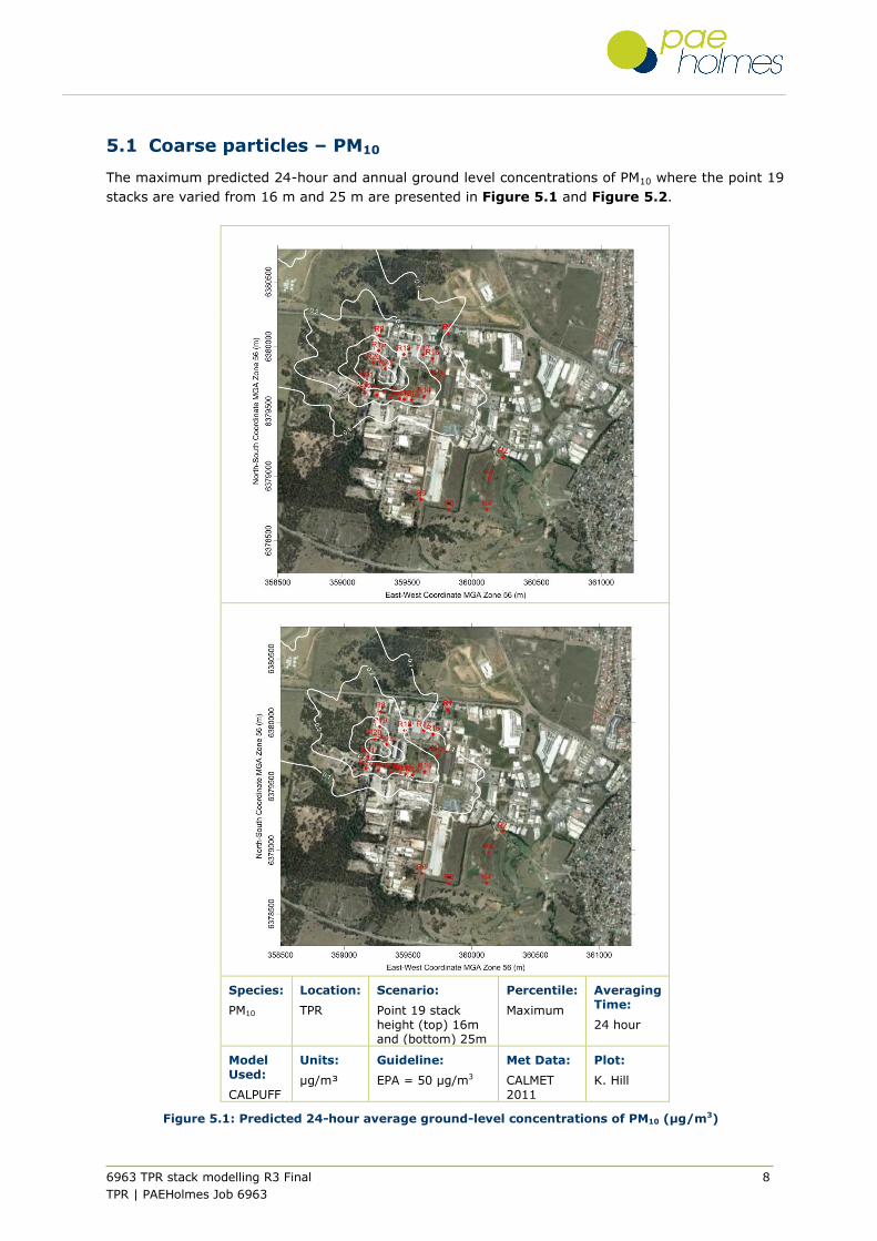
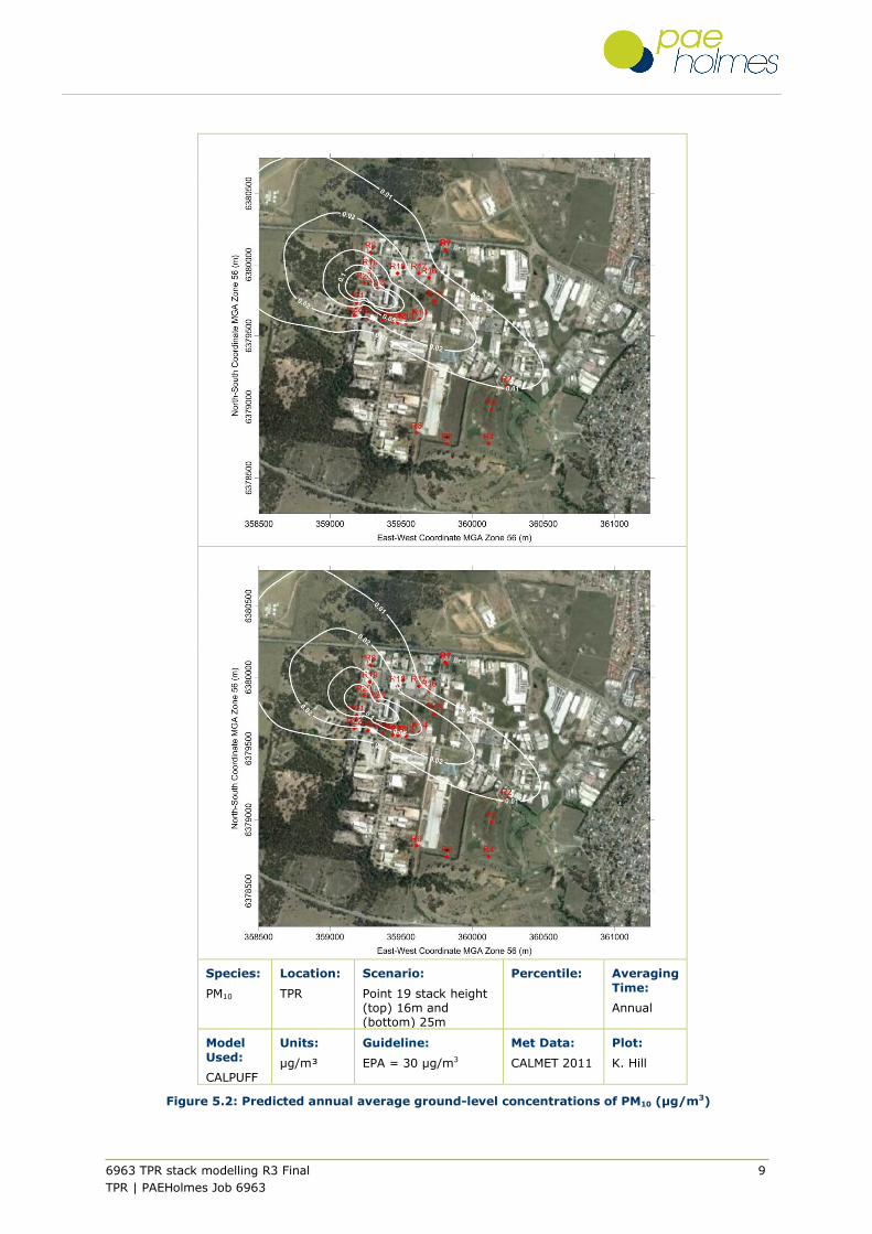
5.1 Coarse particles – PM10

The maximum predicted 24-hour and annual ground level concentrations of PM10 where the point 19

stacks are varied from 16 m and 25 m are presented in Figure 5.1 and Figure 5.2.

Species:

PM10

Location:

TPR

Scenario:

Point 19 stack height (top) 16m and (bottom) 25m

Percentile:

Maximum

Averaging Time:

24 hour

Model Used:

CALPUFF

Units:

µg/m³

Guideline:

EPA = 50 µg/m3

Met Data:

CALMET 2011

Plot:

K. Hill

Figure 5.1: Predicted 24-hour average ground-level concentrations of PM10 (µg/m3)



Species:

PM10

Location:

TPR

Scenario:


Percentile:

Averaging

Time:

Annual

Model

Used:

CALPUFF

Units:

µg/m³

Guideline:

EPA = 30 µg/m3

Met Data:

CALMET 2011

Plot:

K. Hill

Figure 5.2: Predicted annual average ground-level concentrations of PM10 (µg/m3)



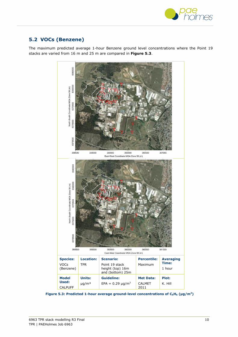
5.2 VOCs (Benzene)

The maximum predicted average 1-hour Benzene ground level concentrations where the Point 19

stacks are varied from 16 m and 25 m are compared in Figure 5.3.

Species:

VOCs (Benzene)

Location:

TPR

Scenario:


Percentile:

Maximum

Averaging

Time:

1 hour

Model

Used:

CALPUFF

Units:

µg/m³

Guideline:

EPA = 0.29 µg/m3

Met Data:

CALMET 2011

Plot:

K. Hill

Figure 5.3: Predicted 1-hour average ground-level concentrations of C6H6 (µg/m3)



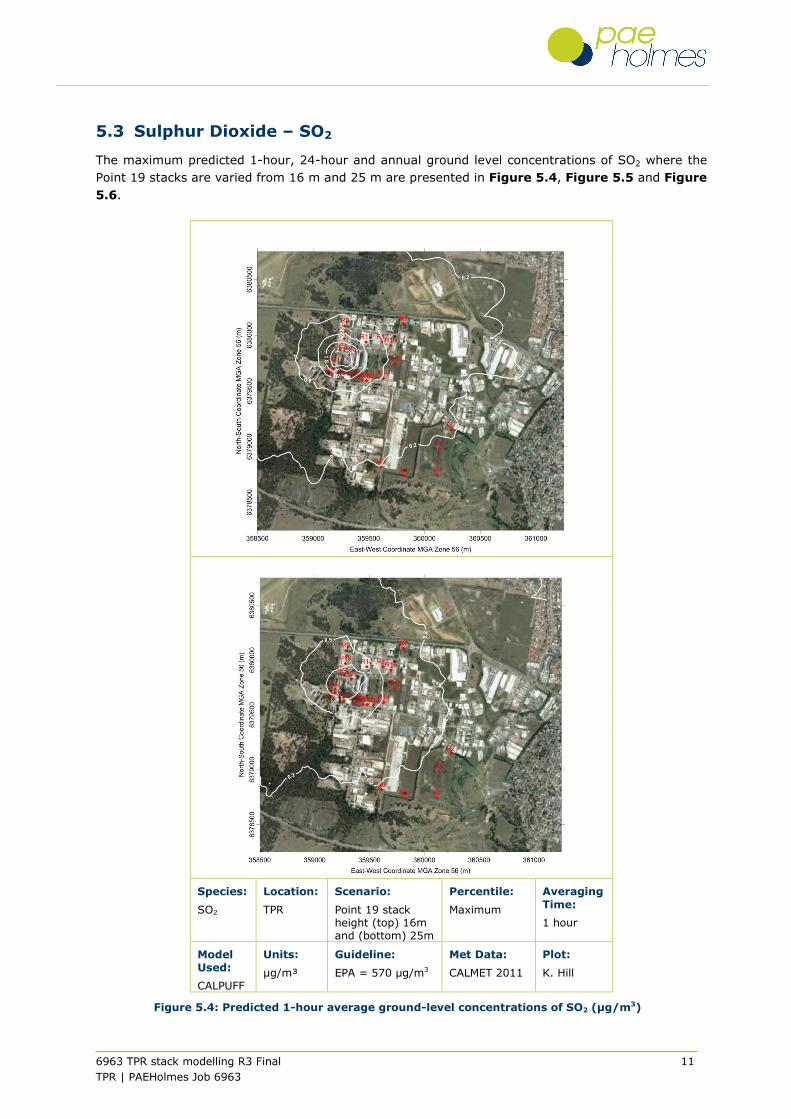
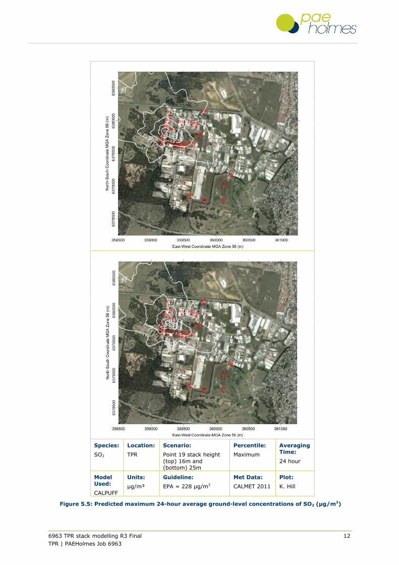
5.3 Sulphur Dioxide – SO2

The maximum predicted 1-hour, 24-hour and annual ground level concentrations of SO2 where the

Point 19 stacks are varied from 16 m and 25 m are presented in Figure 5.4, Figure 5.5 and Figure

5.6.

Species:

SO2

Location:

TPR

Scenario:


Percentile:

Maximum

Averaging

Time:

1 hour

Model

Used:

CALPUFF

Units:

µg/m³

Guideline:

EPA = 570 µg/m3

Met Data:

CALMET 2011

Plot:

K. Hill

Figure 5.4: Predicted 1-hour average ground-level concentrations of SO2 (µg/m3)



Species:

SO2

Location:

TPR

Scenario:

Point 19 stack height

(top) 16m and (bottom) 25m

Percentile:

Maximum

Averaging Time:

24 hour

Model Used:

CALPUFF

Units:

µg/m³

Guideline:

EPA = 228 µg/m3

Met Data:

CALMET 2011

Plot:

K. Hill

Figure 5.5: Predicted maximum 24-hour average ground-level concentrations of SO2 (µg/m3)



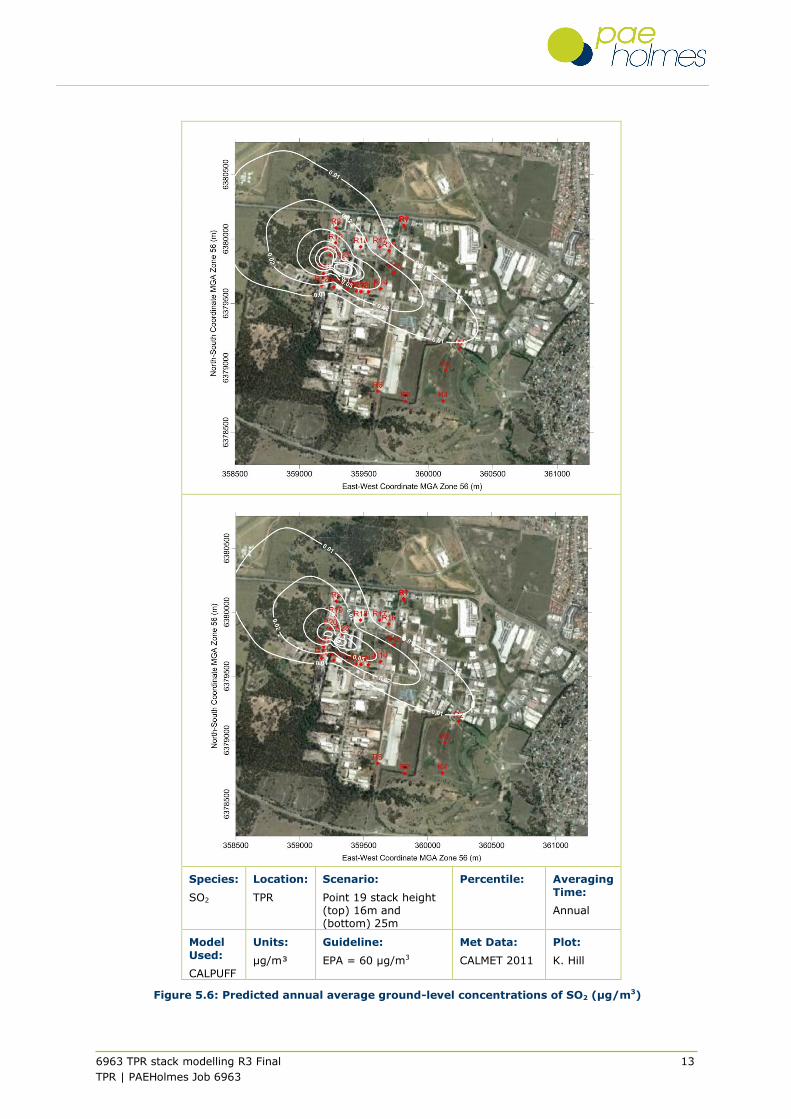
Species:

SO2

Location:

TPR

Scenario:


Percentile:

Averaging

Time:

Annual

Model

Used:

CALPUFF

Units:

µg/m³

Guideline:

EPA = 60 µg/m3

Met Data:

CALMET 2011

Plot:

K. Hill

Figure 5.6: Predicted annual average ground-level concentrations of SO2 (µg/m3)



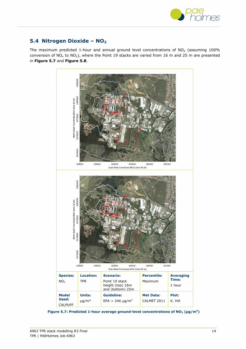
5.4 Nitrogen Dioxide – NO2

The maximum predicted 1-hour and annual ground level concentrations of NO2 (assuming 100%

conversion of NOx to NO2), where the Point 19 stacks are varied from 16 m and 25 m are presented

in Figure 5.7 and Figure 5.8.

Species:

NO2

Location:

TPR

Scenario:


Percentile:

Maximum

Averaging Time:

1 hour

Model Used:

CALPUFF

Units:

µg/m³

Guideline:

EPA = 246 µg/m3

Met Data:

CALMET 2011

Plot:

K. Hill

Figure 5.7: Predicted 1-hour average ground-level concentrations of NO2 (µg/m3)



Species:

NO2

Location:

TPR

Scenario:


Percentile:

Averaging Time:

Annual

Model Used:

CALPUFF

Units:

µg/m³

Guideline:

EPA = 62 µg/m3

Met Data:

CALMET 2011

Plot:

K. Hill

Figure 5.8: Predicted annual average ground-level concentrations of NO2 (µg/m3)



5.5 Hydrogen Sulphide Mist – H2SO4

The maximum predicted 1-hour ground level concentrations of H2SO4 where the Point 19 stacks are

varied from 16 m and 25 m are presented in Figure 5.9.

Species:

H2SO4

Location:

TPR

Scenario:

Point 19 stack

height (top) 16m and (bottom) 25m

Percentile:

Maximum

Averaging Time:

1 hour

Model Used:

CALPUFF

Units:

µg/m³

Guideline:

EPA = 0.018 µg/m3

Met Data:

CALMET 2011

Plot:

K. Hill

Figure 5.9: Predicted 1-hour average ground-level concentrations of H2SO4 (µg/m3)



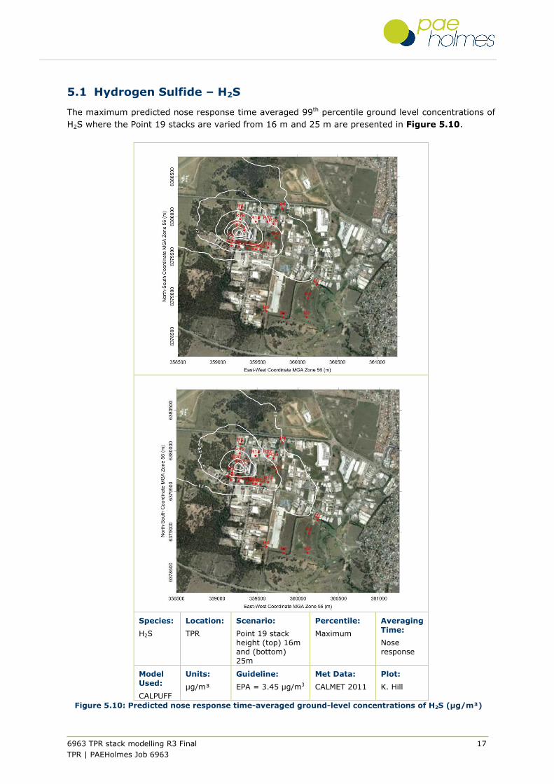
5.1 Hydrogen Sulfide – H2S

The maximum predicted nose response time averaged 99th percentile ground level concentrations of

H2S where the Point 19 stacks are varied from 16 m and 25 m are presented in Figure 5.10.

Species:

H2S

Location:

TPR

Scenario:


Percentile:

Maximum

Averaging

Time:

Nose response

Model

Used:

CALPUFF

Units:

µg/m³

Guideline:

EPA = 3.45 µg/m3

Met Data:

CALMET 2011

Plot:

K. Hill

Figure 5.10: Predicted nose response time-averaged ground-level concentrations of H2S (µg/m³)



6 VARYING STACK PARAMETERS

Further investigation was carried out for five on site receptor locations. Figure 6.1 shows the

locations of these on-site receptors and the six modelling scenarios are listed below.

Scenario 1: 16 m stack, exit velocity 4.7 m/s (current conditions)

Scenario 2: 25 m stack, exit velocity 4.7 m/s

Scenario 3: 16 m stack, exit velocity 7 m/s




These scenarios were run for H2SO4, NOx, H2S and Benzene as these pollutants were those closest to

the air quality goals. The results are presented in Table 9, and the percentage change in ground

level concentrations relative to Scenario 1 are shown in Table 10.

For these five on-site receptors there is very little reduction gained by increasing the exit velocity.

The biggest reductions come from increasing the stack height to 25 m, and the most significant of

these is in the H2SO4 concentrations (up to 45% by increasing to 25 m alone, and 46% for

increasing stack height and exit velocity).



Table 9: Ground level concentrations for each modelling scenario (µg/m3)

Receptor ID Easting Northing H2SO4 NOx 1hr H2S Benzene

Criteria 0.018 246 3.45 0.029

Scenario 1 - 16m stack EV 4.67 m/s

R1 359309 6379756 0.010 38 1.37 0.0008

R2 359310 6379815 0.013 50 1.69 0.0010

R3 359268 6379824 0.014 52 1.87 0.0010

R4 359256 6379764 0.009 38 1.17 0.0011

R5 359311 6379839 0.010 42 1.30 0.0007


R1 359309 6379756 0.006 30 1.32 0.0008

R2 359310 6379815 0.007 36 1.56 0.0010

R3 359268 6379824 0.008 38 1.86 0.0010

R4 359256 6379764 0.008 34 1.13 0.0011

R5 359311 6379839 0.007 27 1.09 0.0007

Scenario 3 - 16m stack EV 7 m/s

R1 359309 6379756 0.010 37 1.37 0.0008

R2 359310 6379815 0.012 49 1.67 0.0010

R3 359268 6379824 0.014 51 1.87 0.0010

R4 359256 6379764 0.009 38 1.17 0.0011

R5 359311 6379839 0.009 41 1.29 0.0007


R1 359309 6379756 0.006 30 1.32 0.0008

R2 359310 6379815 0.007 36 1.56 0.0010

R3 359268 6379824 0.008 38 1.86 0.0010

R4 359256 6379764 0.008 34 1.13 0.0011

R5 359311 6379839 0.007 27 1.09 0.0007


R1 359309 6379756 0.010 36 1.37 0.0008

R2 359310 6379815 0.012 46 1.65 0.0010

R3 359268 6379824 0.014 52 1.87 0.0010

R4 359256 6379764 0.009 38 1.17 0.0011

R5 359311 6379839 0.009 38 1.24 0.0007


R1 359309 6379756 0.006 30 1.32 0.0008

R2 359310 6379815 0.007 36 1.56 0.0010

R3 359268 6379824 0.008 38 1.86 0.0010

R4 359256 6379764 0.008 34 1.13 0.0011

R5 359311 6379839 0.007 27 1.09 0.0007



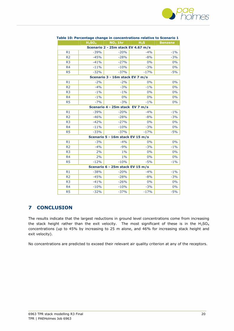
Table 10: Percentage change in concentrations relative to Scenario 1

H2SO4 NO2 1hr H2S Benzene


R1 -39% -20% -4% -1%

R2 -45% -28% -8% -3%

R3 -41% -27% 0% 0%

R4 -11% -10% -3% 0%

R5 -32% -37% -17% -5%


R1 -2% -2% 0% 0%

R2 -4% -3% -1% 0%

R3 -1% -1% 0% 0%

R4 -1% 0% 0% 0%

R5 -7% -3% -1% 0%


R1 -39% -20% -4% -1%

R2 -46% -28% -8% -3%

R3 -42% -27% 0% 0%

R4 -11% -10% -3% 0%

R5 -33% -37% -17% -5%


R1 -3% -4% 0% 0%

R2 -4% -9% -3% -1%

R3 2% 1% 0% 0%

R4 2% 1% 0% 0%

R5 -12% -10% -5% -1%


R1 -38% -20% -4% -1%

R2 -45% -28% -8% -3%

R3 -41% -26% 0% 0%

R4 -10% -10% -3% 0%

R5 -32% -37% -17% -5%

7 CONCLUSION

The results indicate that the largest reductions in ground level concentrations come from increasing

the stack height rather than the exit velocity. The most significant of these is in the H2SO4

concentrations (up to 45% by increasing to 25 m alone, and 46% for increasing stack height and

exit velocity).

No concentrations are predicted to exceed their relevant air quality criterion at any of the receptors.



8 REFERENCES

DEC (2005)

“Approved Methods for the Modelling and Assessment of Air Pollutants in New South Wales”.

New South Wales EPA.

NEPC (1998)

“National Environmental Protection Measure and Impact Statement for Ambient Air Quality”.

National Environment Protection Council Service Corporation, Level 5, 81 Flinders Street,

Adelaide SA 5000.

Documents

STACK MODELLING FOR TRANSPACIFIC REFINERS, RUTHERFORD