0

Transpacific Trade Imbalances: Causes and Cures*

Jong-Wha Lee

Korea University and The Australian National University

Warwick J. McKibbin The Australian National University

and The Lowy Institute for International Policy and The Brookings Institution

and Yung Chul Park

Korea University

Revised: June 2005 Abstract

This paper explores the causes of the transpacific trade imbalances using an empirical global model. It also evaluates the impact of various policies to reduce these imbalances. We find the fundamental cause of trade imbalance since 1997 is changes in saving-investment gaps, attributed to the surge of the U.S fiscal deficits and the decline of East Asia’s private investment after the 1997 financial crisis. Our simulation results show that a revaluation of East Asia’s exchange rates by 10 percent (effectively a shift in monetary policy) cannot resolve the imbalances. We find East Asia’s concerted efforts to stimulate aggregate demand can have significant impacts on trade balances globally, but the impact on the US trade balance is not large. US fiscal contraction is estimated to have large impacts on the US trade position overall and on the bilateral trade balances with East Asian economies. These results suggest that in order to improve the transpacific imbalance, macroeconomic adjustment will need to be made on both sides of the Pacific. Keywords: Current Accounts, US Trade Deficit, Exchange Rate Policy, East Asia, Multi-country Simulation Model. JEL Classification Codes: F32, F42, 05

* We thank Eduardo Borensztein and other participants at the session, “Global Imbalances and East Asia’s Exchange Rate Policy”, at the Western Economic Association International Annual Conference, Vancouver Canada, June 30 2004, for helpful comments, and Jongduk Kim for research assistance. We also thank anonymous referees of this journal for helpful comments. .

1

1. INTRODUCTION

Global trade imbalances continue to enlarge. The US current account deficit has

widened significantly. In contrast, China, Japan and East Asian emerging economies

including Hong Kong SAR, Korea, Singapore and Taiwan have persistently

accumulated large current account surpluses, the bulk of which has come from their

trade with the United States. The size of East Asia’s current account surpluses has led to

massive accumulation of dollar reserves, given strong foreign exchange market

intervention by East Asian central banks.

In managing exchange rate policy, China, Hong Kong, and Malaysia have maintained a

fixed parity vis-à-vis the US dollar. Other countries including Japan, Korea, and

Singapore rely on de jure floating exchange rate systems, but in practice have

intervened extensively in the foreign exchange market to maintain competitiveness of

the export sector.

The growing imbalances between regions across the Pacific have provoked heated

debates. What contributed to the transpacific imbalances? What will be the

consequences of these imbalances? If it is desirable to reduce these imbalances what

would be feasible policies to correct for the imbalances? The purpose of this paper is to

analyze these issues.

In recent studies, Dooley, Folkerts-Landau and Garber (2003, 2004) argue that East

Asia’s export-led strategy is the principle cause of the growing global imbalance or that

2

it will block the adjustment that will reduce the transpacific imbalance. Some US

government officials argue that East Asian countries, notably China, should abandon the

strategy of exchange rate undervaluation and increase exchange rate flexibility in order

to share the burden of global readjustments. Eichengreen and Park (2004) assert that an

increase in public investment by East Asian economies would help to stimulate

domestic demand and reduce their current account surpluses.

This paper explores the effects of these proposed policies on the transpacific imbalances.

This paper attempts to provide empirical estimates for the effects of the proposals based

on a simulation model which is better equipped in assessing the dynamic effects of

policy changes. Our experiments are based on a multi-country intertemporal general

equilibrium model called the Asia-Pacific G-cubed Model (see McKibbin and Wilcoxen,

1998). This model incorporates important linkages between countries and regions,

through trade and capital flows, which is the key element to assess the sources of global

imbalances or the effects of polices to eliminate transpacific imbalance.

The major finding of the simulation exercises is that a concerted revaluation of East

Asian exchange rates by 10 percent could not make any sustained significant impact on

the trade imbalances. Changes in Asian fiscal policies or investment rates in Asia can

have significant impacts on their trade balances, but their impact on the US trade

balance is not large. A reduction in U.S. fiscal deficits can be more effective to deal with

the U.S. current account deficit, and reduce the transpacific imbalance.

The paper is structured as follows. Section 2 discusses the causes and development of

3

the imbalances. Section 3 discusses the implications of the imbalances for East Asian

economies and suggests policies to reduce the imbalances. Section 4 introduces the

dynamic model that is used for evaluating the effects of the proposed policies. Section 5

provides empirical results based on simulation experiments from the model. Concluding

remarks follow in the final section.

2. THE CAUSES AND DEVELOPMENT OF GLOBAL IMBALANCES

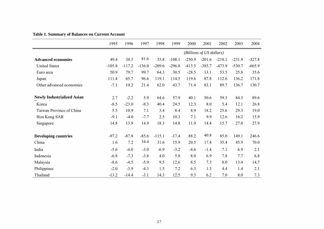
The United States current account deficit has increased significantly in recent years. In

2004, the US deficit stood at $666 billion, up from $136 billion in 1997. It amounted to

5.7 percent of GDP, increasing from 1.6 percent seven years earlier (Table 1).

The current accounts in East Asian economies have mirrored that of the United States.

Japan and four East Asian NIES (newly industrialized economies) including Hong Kong

SAR, Korea, Singapore and Taiwan have persistently accumulated large amounts of

surplus on their current accounts (Table 1). In 2004, Japan had a current account surplus

of $172 billion, amounting to 3.7 percent of GDP, and the four East Asian emerging

economies as a group had a surplus of $90 billion, or 7.1 percent of their GDP. China

also had a surplus of about $70 billion in 2004 or 4.2 percent of GDP. A significant

portion of East Asia’s current account surpluses originated from the region’s trade with

the U.S. In 2004, US trade deficit with 10 East Asian countries including Japan and

China amounted to $ 284 billion (see Table 2).

The principal cause of the US current account deficits is the low levels of private and

4

public saving rates relative to investment in the United States. In 2003 the US gross

private saving rate remained at 13.6 percent of GDP. The private saving rates dropped

continuously from over 19 percent in 1980s to 14 percent in 2001. In particular, the

recent worsening of the US current account deficits reflects the deterioration of public

savings. Over the period between late 80s and 2001, the US fiscal balance improved

dramatically from negative savings to positive, peaking at 4.4 percent of GDP in 2000.

However, in 2002 fiscal saving switched back to negative, –0.2 percent of GDP, as the

US government loosened fiscal policy beginning from early 2001 as the US economy

was heading towards a recession. The US government adopted a series of significant tax

cuts. There was a considerable amount of fiscal stimulus from spending increases as

well. The federal government budget balance (including the social security surplus)

shifted from a surplus of 2.5 per cent of GDP in FY 2000 to a deficit of more than 4 per

cent of GDP in FY 2004.1 In 2004 the US public saving rate is estimated to be –2.2

percent of GDP.

As the massive US current account deficit is attributed to its low savings relative to

investment, the East Asian current account surpluses reflect high saving rates relative to

investment in East Asia. In 2003, the national saving rate was 26 percent in Japan, and

23 percent in a group of four East Asian emerging economies. The public saving rate

was 0.5 percent and 5.7 percent in Japan and four East Asian emerging economies

respectively.

While the high saving rates in East Asia must have contributed to the prolonged global

1 See Council of Economic Advisors (2003) and Muhleisen and Towe (2004) for details.

5

imbalances, the recent surge of surpluses reflects a reduction in domestic demand in this

region. After the financial crisis of 1997, investment as a proportion of GDP fell in most

East Asian countries, and has not yet recovered.2 In a group of four East Asian NIES,

investment rates dropped from 31.6% in 1997 to 23.0 % of GDP in 2003. Indonesia,

Malaysia and Thailand experienced a fall in investment ratio amounting to about 20

percentage points (Table 3).

Since 1998, interest rates have fallen to historically low levels, leaving little room for

additional monetary expansion. East Asia has traditionally valued fiscal prudence highly,

and with the IMF on the watch these countries have not seriously considered fiscal

expansion as a means of expanding domestic demand. In four East Asia NIES, public

investment has declined from 9.6% in 1997 to 6.2 % of GDP in 2002.

Although the worst of the crisis was over by 2000, many of the East Asian economies

found themselves with large underutilized capacity in manufacturing and vacant

commercial and residential buildings that were constructed before the crisis. The

existing excess capacity, despite the sharp decline in real interest rates, has held back

new investment in many East Asian countries (Park, 2004). In recent years, the capital

intensity of Asian exports has also declined as the region has shifted to exporting more

IT industry products and services that are skill and knowledge intensive than before.

This shift has also contributed to weaker investment demand.

2 Barro and Lee (2003) analyzes the movements of investment and growth in East Asia before and after

the financial crisis of 1997 and claims that the financial crisis would have permanent depressing effects

on investment.

6

The combination of substantial changes in savings and investment in Asia and the

United States explains much of the transpacific imbalances.

3. IMPLICATIONS AND POLICY CHALLENGES OF THE TRADE AND FINANCIAL IMBALANCES

a. East Asia’s ‘Export-led Growth’ Policy

Fiscal policy in the United States has been very expansionary, and is projected to remain

extremely loose in the next decade (Muhleisen and Towe, 2004). In theory the persistent

U.S. twin deficits should ultimately lead to real depreciation of the US dollar and an

increase in U.S. interest rates, thereby helping the deficits to diminish. Nevertheless, the

US deficits have been sustained, and there have been almost no significant forces

toward reducing the global imbalances.

In a series of influential articles, Dooley, Folkerts-Landau and Garber (2003, 2004)

contend that the imbalance can be sustained for a long time as long as East Asian

economies continue to follow an ‘export-led growth’ strategy. In their view, the U.S.

trade deficits have persisted because East Asia is willing to finance them by

accumulating an unlimited amount of dollar reserve assets in order to keep exchange

rates undervalued.

7

East Asian countries, with underdeveloped financial markets and a ‘fear of floating’

against the US dollar, have intervened heavily in the foreign exchange market so as to

moderate excessive volatility of exchange rates, but mostly to maintain competitiveness

of export sectors. The intervention is reflected in the stability of real exchange rates in

East Asian economies in recent years. The international reserves of 10 East Asian

economies increased significantly in recent years, amounting to 1.8 trillion US dollars.

Dooley et al. named the current situation as a ‘revived Bretton Woods system’, where

East Asian countries peg to the center’s currency, the US dollar, as the European

countries did under Bretton Woods. The periphery countries hoard their export earnings

in low-yielding US Treasuries and other dollar denominated assets in order to maintain

exchange rates stable vis-à-vis the US dollar. While the reserve accumulation is costly

to the East Asian economies, the export-led growth can be a (sub-)optimal choice for the

countries in the periphery considering the lower productivity in non-tradable sectors.

East Asian’s craving for dollar assets must have helped the U.S. current account

imbalances persist or more importantly affected the price at which these imbalances are

sustainable. However, it is incorrect to argue that East Asia’s exchange rate policy is the

principle cause of the growing global imbalances. Many East Asian countries ran large

current account deficits in the course of promoting exports before the crisis. As

explained in the earlier section, much of the increase in current account surpluses since

the crisis is explained by a sharp reduction in domestic investment demand while

domestic saving as a proportion of GDP has remained largely unchanged in East Asia.

8

Immediately after the 1997-98 crisis, exports provided the only way out of the crisis and

of sustaining recovery to the crisis-hit Asian countries, as these countries were not able

to expand domestic demand by implementing expansionary monetary and fiscal policy

in the midst of crisis management. Unable to stimulate domestic demand, East Asian

countries have been driven to rely on exports to sustain a fledgling recovery. Most East

Asian countries had put in place a system of promoting an export-led growth strategy

before the crisis, and it was perhaps natural then that they turned to exports as the major

source of growth. Most East Asian countries have also had to generate current account

surpluses to replenish the foreign exchange reserves they lost in the run-up to the crisis .

The continuing pursuit of interventionist exchange rate regimes and reserve

accumulation has created serious problems for the East Asian economies. The distortion

of real exchange rates has discouraged investment in the non-tradable sector, creating

unbalanced growth of the economy. The de facto pegging exchange rate system

combined with deregulated capital market leaves little room for independent monetary

policy as manifested by the ‘impossible trinity’.

The export-led growth strategy also has other undesirable side effects. The continuing

accumulation of foreign assets would not be always successfully sterilized. A

subsequent increase in the supply of money is bound to be translated into inflation of

goods and services or real and financial assets. While price increases have been modest

so far in East Asia, it is inevitable that amassed current account surpluses and net capital

inflows will induce rising inflation. In particular recent data for China suggest a

significant acceleration in inflation.

9

The intervention in foreign exchange markets to keep exchange rates undervalued could

precipitate a round of boom-and-bust cycles. The capital inflows and current surpluses

have generated expectations of currency appreciation and cause further capital inflows,

thereby amplifying a cyclical upswing in real asset prices. But then once capital

outflows happen, it could trigger a significant collapse of asset prices.

b.What Can Be Done by East Asia?

Should East Asia stop its pursuit of the ‘export-led growth’ strategy? Some US

government and international financial institutions officials have argued that East Asian

countries should abandon their interventionist exchange rate regime and increase

exchange rate flexibility in order to alleviate global imbalances.

The demand for an appreciation of currencies in East Asia raises several fundamental

questions. One is the collective action problem that unless both China and Japan are

prepared to let their currencies appreciate, other countries will not follow. Park (2004)

argues that an independent revaluation by individual East Asian countries will lead to

loss of relative currency competitiveness in the current situation in which there is a lack

of coordination of exchange policies among East Asian countries. It is uncertain that

China can move first to make upward discrete adjustments of the Renminbi or

eventually go for a more flexible exchange rate regime. Chinese policy makers would

not give up pegging the exchange rate at a competitive level as long as they believe that

10

they need to support their export industries and thereby promote employment and

output growth. In addition, the bilateral trade imbalances between countries in the

region add more complications. Most of the Asian economies, while competing with

China in third markets, have recorded trade surpluses with China. Thus, Chinese

revaluation will exert mixed effects on other Asian economies (as illustrated below). In

the case of Japan, further strengthening of the yen would aggravate its deflation problem

and hurt the economy which is now recovering from a long recession.

Another issue is the extent to which an appreciation of East Asian currencies will reduce

the transpacific imbalance. The impact depends very much on the source of the currency

appreciation – whether it was a currency adjustment effectively as a change in monetary

policy or whether it was brought about through other policy changes. Even if East Asian

countries including Japan were able to agree to a region-wide currency adjustment, it is

not clear whether the adjustment would lead to a sizable reduction in East Asia’s

aggregate current account surplus. Many analysts argue that an appreciation of the East

Asian currencies across the board on the order of, for example, five to ten percent on

average will not have much impact on the transpacific imbalance (Eichengreen, 2004).

This is clearly an empirical question. We seek for an answer to this question in the next

section.

East Asian economies can adopt polices to stimulate their aggregate demand. However,

what really matters for current account balances is how these demand policies impact on

savings relative to investment in Asian economies. Although economic recoveries have

occurred, many crisis-hit East Asian economies have not recovered their pre-crisis

11

investment ratio. But, with historically low real interest rates and increasing inflation

pressures, many East Asian governments have little room to implement expansionary

monetary policy and thereby stimulate private spending. Unable to expand demand by

monetary policy, they can consider fiscal expansion as another means regardless of its

effectiveness.

Eichengreen and Park (2004) suggest that fiscal expansion is a feasible policy that East

Asian countries except Japan can consider in reducing global imbalances. They assert

that regionally concerted efforts to increase public spending by East Asian economies

help to revive domestic demand and non-tradable sectors, resulting in real exchange rate

appreciation and decrease in current account surpluses.

What is uncertain is that a reduction in East Asia’s surplus may not necessarily lead to a

corresponding reduction in the US current account deficit. The effects on the US current

account are not likely to be a large fraction of their own GDP because the size of the

expanding countries is small relative to the United States. Moreover, a decline in East

Asia’s surplus may occur as East Asian countries start importing more from Europe and

other non-US regions, while exporting less. If this happens, it can further complicate

global adjustments involving the US, Europe, and Asia.

4. EFFECTS OF ADJUSTMENT POLICES

a.The G-Cubed (Asia Pacific) Model

Given the important linkages between affected countries in the region, through the trade

12

of goods and services and capital flows, any analysis of the sources of global

imbalances or policies to reduce imbalances needs to be undertaken with a model that

adequately captures these interrelationships. The G-Cubed (Asia Pacific) model is a 6

sector version of the G-Cubed model outlined in McKibbin and Wilcoxen (1998).

This model is ideal for such analysis having both detailed country coverage of

the region and rich links between countries through goods and asset markets. 3 A

number of studies—summarized in McKibbin and Vines (2000)—show that the G-

cubed/MSG3 models have been useful in assessing a range of issues across a number of

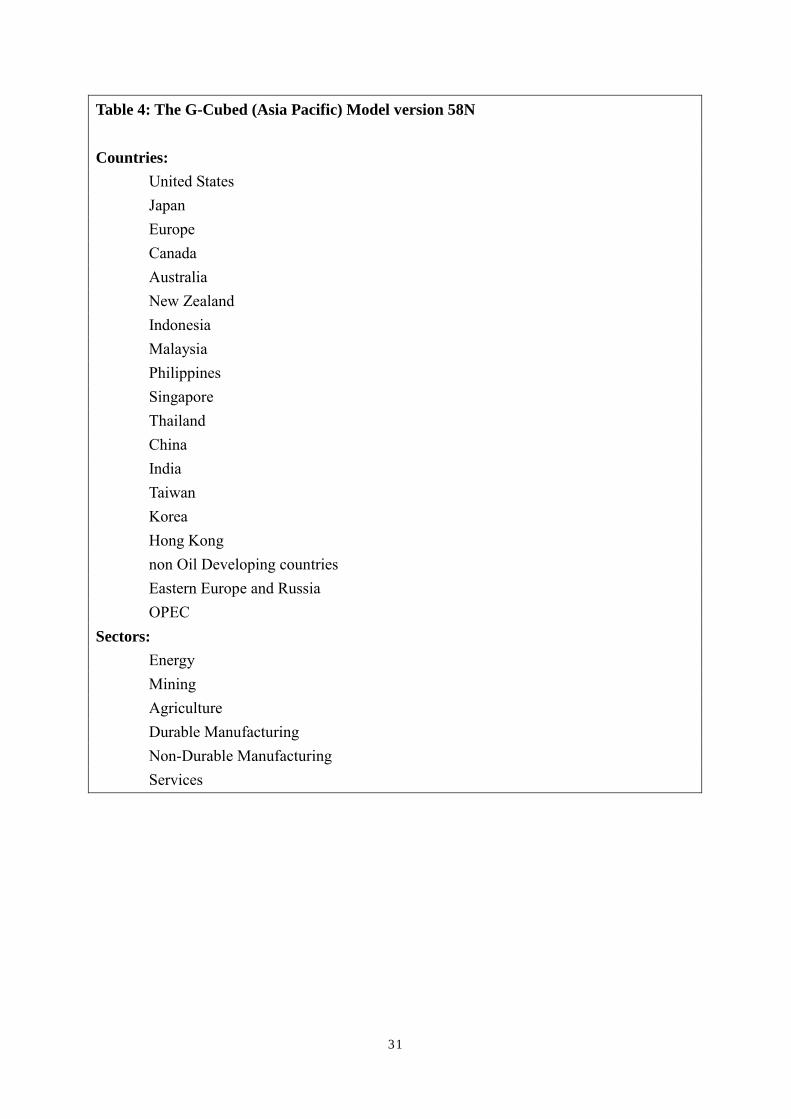
countries since the mid-1980s.4 A summary of the model coverage is presented in

Table 4. Some of the principal features of the model are as follows:

● The model is based on explicit intertemporal optimization by the agents

(consumers and firms) in each economy5. In contrast to static CGE models, time and

dynamics are of fundamental importance in the G-Cubed model.

● In order to track the macro time series, however, the behavior of agents is

modified to allow for short run deviations from optimal behavior either due to myopia

or to restrictions on the ability of households and firms to borrow at the risk free bond

rate on government debt. For both households and firms, deviations from intertemporal

optimizing behavior take the form of rules of thumb, which are consistent with an 3 Full details of the model including a list of equations and parameters can be found online at:

www.gucubed.com 4 These issues include: Reaganomics in the 1980s; German Unification in the early 1990s; fiscal

consolidation in Europe in the mid-1990s; the formation of NAFTA; the Asian crisis; and the productivity

boom in the US. 5 See Blanchard and Fischer (1989) and Obstfeld and Rogoff (1996).

13

optimizing agent that does not update predictions based on new information about

future events. These rules of thumb are chosen to generate the same steady state

behavior as optimizing agents so that in the long run there is only a single intertemporal

optimizing equilibrium of the model. In the short run, actual behavior is assumed to be a

weighted average of the optimizing and the rule of thumb assumptions. Thus aggregate

consumption is a weighted average of consumption based on wealth (current asset

valuation and expected future after tax labor income) and consumption based on current

disposable income. Similarly, aggregate investment is a weighted average of investment

based on Tobin’s q (a market valuation of the expected future change in the marginal

product of capital relative to the cost) and investment based on a backward looking

version of Q.

● There is an explicit treatment of the holding of financial assets, including money.

Money is introduced into the model through a restriction that households require money

to purchase goods.

● The model also allows for short run nominal wage rigidity (by different degrees

in different countries) and therefore allows for significant periods of unemployment

depending on the labor market institutions in each country. This assumption, when taken

together with the explicit role for money, is what gives the model its “macroeconomic”

characteristics. (Here again the model's assumptions differ from the standard market

clearing assumption in most CGE models.)

● The model distinguishes between the stickiness of physical capital within

14

sectors and within countries and the flexibility of financial capital, which immediately

flows to where expected returns are highest. This important distinction leads to a critical

difference between the quantity of physical capital that is available at any time to

produce goods and services, and the valuation of that capital as a result of decisions

about the allocation of financial capital.

As a result of this structure, the G-Cubed model contains rich dynamic behavior, driven

on the one hand by asset accumulation and, on the other by wage adjustment to a

neoclassical steady state. It embodies a wide range of assumptions about individual

behavior and empirical regularities in a general equilibrium framework. The

interdependencies are solved out using a computer algorithm that solves for the rational

expectations equilibrium of the global economy. It is important to stress that the term

‘general equilibrium’ is used to signify that as many interactions as possible are

captured, not that all economies are in a full market clearing equilibrium at each point in

time. Although it is assumed that market forces eventually drive the world economy to a

neoclassical steady state growth equilibrium, unemployment does emerge for long

periods due to wage stickiness, to an extent that differs between countries due to

differences in labor market institutions.

5. SIMULATION RESULTS

a.Baseline Business-As-Usual Projections

To solve the model for each year from 2002 to 2081, we first normalize all

quantity variables by each economy's endowment of effective labor units. This means

that in the steady state all real variables are constant in these units although the actual

levels of the variables will be growing at the underlying rate of growth of population

15

plus productivity. Next, we must make base-case assumptions about the future path of

the model's exogenous variables in each region. In all regions we assume that the long

run real interest rate is 5 percent, tax rates are held at their 2002 levels and that fiscal

spending is allocated according to 2002 shares. Population growth rates vary across

regions as per the 2000 World Bank population projections.

A crucial group of exogenous variables are productivity growth rates by sector

and country. The baseline assumption in the MSG3 model is that the pattern of technical

change at the sector level is similar to the historical record for the United States (where

data is available). In regions other than the United States, however, the sector-level rates

of technical change are scaled up or down in order to match the region’s observed

average rate of aggregate productivity growth over the past 5 years. This approach

attempts to capture the fact that the rate of technical change varies considerably across

industries while reconciling it with regional differences in overall growth. This is clearly

a rough approximation; if appropriate data were available it would be better to estimate

productivity growth for each sector in each region.

Given these assumptions, we solve for the model's perfect-foresight equilibrium

growth path over the period 2002-2081. This a formidable task: the endogenous

variables in each of the 80 periods number over 2500 variables and include, among

other things: the equilibrium prices and quantities of each good in each region,

intermediate demands for each commodity by each industry in each region, asset prices

by region and sector, regional interest rates, bilateral exchange rates, incomes,

investment rates and capital stocks by industry and region, international flows of goods

and assets, labor demanded in each industry in each region, wage rates, current and

capital account balances, final demands by consumers in all regions, and government

16

deficits.6 At the solution, the budget constraints for all agents are satisfied, including

both intra-temporal and inter-temporal constraints. We need to solve the model for a

longer than our period of interest (a decade) because of the assumption of rational

expectations in some markets which implies that adjustment of stocks in future period

impact on the calculation of asset prices in the short run.

b. The simulations

We now consider a range of shocks and how these shocks impact on the global economy.

The shocks we consider are shocks that might explain the changes in global trade balances

in the past decade as well as possible policy changes that might impinge on these trade

balances in future years. They are stylized representations of what has been observed rather

than precise estimates so as to illustrate the rough orders of magnitude of effects (which in a

dynamic model change over time). We could solve the model from an earlier period but the

calculation of percentage changes would be little different from what we find starting from

2002. It is important not to read the results too precisely because we are only approximating

the shocks rather than attempting to recreate history7.

1) Asian private investment shock: a permanent rise of 0.5% in the equity risk premium

in Japan, 2% in Indonesia, and 1% in other Asian economies except China sufficient

6 Since the model is solved for a perfect-foresight equilibrium over a 80 year period, the numerical

complexity of the problem is on the order of 80 times what the single-period set of variables would

suggest. We use software summarized in McKibbin and Sachs (1991) Appendix C, for solving large

models with rational expectations on a personal computer. 7 Chapter 5 of McKibbin and Sachs (1991) use a similar model to recreate the 1980s but that is a massive

task in a rational expectations model. The exercise here is meant to give broad orders of magnitude

multipliers for various shocks.

17

to reduce private investment rates by the extent observed between 1997 and 2002,

and an decrease of 0.5% in the equity risk premium in China reflecting the Chinese

investment boom;8

2) U.S. fiscal deficit shock: A permanent rise in the US fiscal deficit of 4% of GDP

comprising a rise in spending in goods and services of 1% of GDP, rise in spending

on labor of 1% of GDP, and a cut in personal income taxes to sufficiently reduce

revenues by 2% of GDP;

3) Asian revaluation shock: A 10% appreciation of the currencies of China, Hong Kong

and other crisis-hit Asian economies such as Indonesia, Korea, Malaysia, the

Philippines, and Thailand9;

4) Asian fiscal expansion shock: A permanent expansion of Asian fiscal deficits

(excluding Japan) of 2% of GDP comprising an increase in spending of 1% of GDP

on goods and services and 1% on labor

c. Results

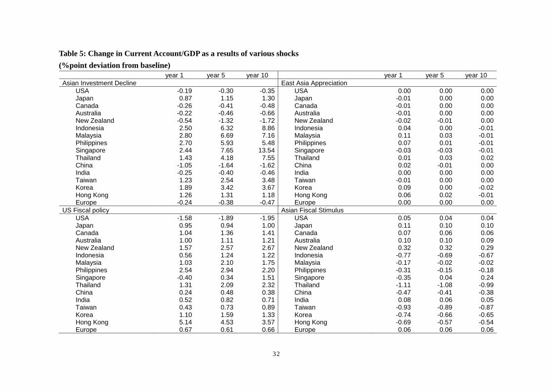
(i) Fall in Asian Investment

Results are presented for changes in current account balances as a percent of GDP

8 We assume the rise in equity risk premium, instead of country risk premium (see McKibbin (1998)),

considering that the shocks have had depressing effects mainly on private domestic investment, rather

than total investment. Evidence shows that in the crisis-hit East Asian countries, country risk premia

increased sharply with the eruption of the crisis in 1997, but then have quickly returned to the pre-crisis

level. 9 In China and Hong Kong this is an instant appreciation since they follow exact pegs – in the other

countries the targeted exchange rate is appreciated by 10% but the actual exchange rate appreciates less

quickly because the exchange rate is only one factor in their monetary reaction functions – in practice

7.5% of the full appreciation has occurred by year 2.

18

(table 5); the percent change in private investment relative to baseline (Table 6); the change

in real effective exchange rates relative to baseline (defined as an increase being an

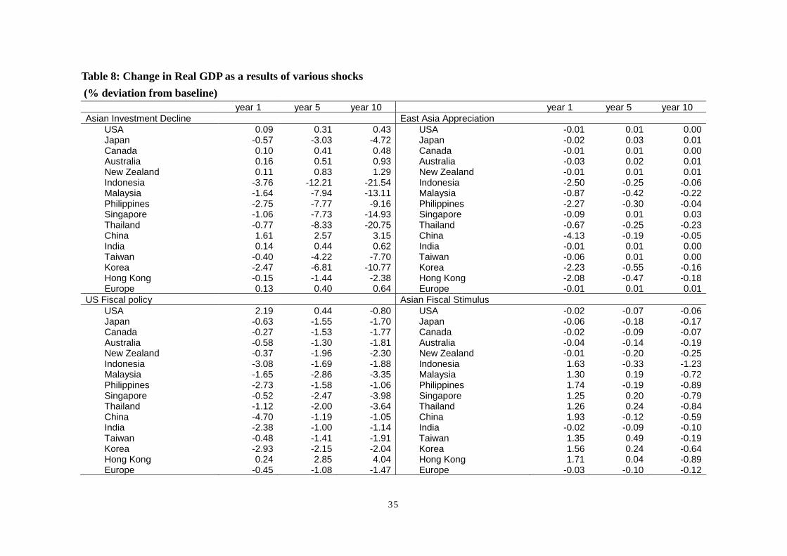
appreciation) (Table 7) and the percent change in real GDP relative to baseline (Table 8).

These tables contain results at year 1, 5 and 10 following the shocks indicated.

The rise is equity risk premia in Asia acts to reduce private investment in Asia. In

the first year, private investment declines by between 5% and 14% relative to baseline, and

the negative impacts on investment are magnified over time due to the permanent nature of

the shocks. In the five years following the shocks, the investment declines range from 13%

(Japan) to 50% (Indonesia). 10This leads to a continuous capital outflow and a depreciation

in effective exchange rates which improves current account balances of Asian economies

except China by between 1.2 and 2.8 percent of GDP in the first year and by between 1.3

and 7.6 percent of GDP by year 5. The capital inflow into the US worsens the US current

account balance by 0.2 percent of GDP in year 1 and 0.3 percent of GDP by year 5. The

reallocation of global capital tends to reduce investment in the economies experiencing the

rise in risk and increase investment in economies receiving the capital that flows out of Asia

(US, other OECD economies as well as China and India).

As expected the fall in real investment in Asian economies reduces GDP in the

economies (table 7) despite the rise in net exports that accompanies the real exchange rate

depreciations in Asia. The opposite is true in the United States where the stronger real

exchange rate lowers net exports but the fall in long term real interest rates driven by the

10 We can convert the estimated declines in the investment levels into the changes in investment rates by

using the actual investment rates in 1997, in table 3, as a base year, and then taking account of the

estimated declines in GDP. A typical case of an Asian economy with the estimated decline of investment

level by 25%, combined with the about 7% GDP decline, after 5 years following the shock of the 1%

increase in the equity risk premium implies a drop of investment ratio from 32% to 26%.

19

capital inflow stimulates private investment by more than the fall in net exports, causing US

real GDP to rise.

These results show that the fall in private investment in Asia since the crisis has

contributed significantly to the size of trade surpluses in Asia but less to the worsening US

trade position.

(ii) US Fiscal Expansion

Results for a permanent increase in US Fiscal deficits are contained in the lower left

panel of Tables 5 through 8. The rise in US fiscal deficits lowers US national savings by

more than national investment and causes a large capital inflow. This inflow which

appreciates the US dollar causes the current account balance to worsen by 1.6% of GDP in

the first year and 1.9% after 5 years. The gradual turn around in the US trade balance

ultimately towards surplus is caused by the requirement that the US external position satisfy

the intertemporal budget constraint that countries must service external debts. The current

account remains in deficit much longer than the trade deficit. The large capital inflow to the

US is reflected in a large capital outflow from other economies. This results in

improvements in trade balance globally and particularly in Asia. The Japanese trade surplus

is 1% higher in the first year of the fiscal package in the US. China experiences less of an

initial trade surplus because of the assumption of a peg to the US dollar which initially

worsens Chinese competitiveness relative to other managed floating Asian economies.

The impact on investment and savings is quite interesting. In the United States the

rise in spending and cut in taxes initially stimulates private consumption and real GDP (table

8) but despite the higher demand, higher long term real interest rates cause investment to

initially rise only slightly and then over time to fall in the United States. The larger fall in

20

investment over time in the United States occurs because the private sector is forced to

reduce private spending in order to finance the permanently higher public spending and tax

cuts that foreigners are increasingly unwilling to service. The only way this would not occur

would be if the higher fiscal deficits created additional aggregate supply sufficient to cover

the permanently higher fiscal deficits. Interestingly the expansionary US fiscal policy is

large enough to raise global long term real interest rates (relative to base) and reduce

investment rates globally in order to finance the US fiscal deficit (Table 6). Indeed the initial

impacts on investment are larger outside the United States because of the initially higher

aggregate demand in the US from the larger fiscal spending.

The US fiscal expansion appreciates the US dollar by 8 percent relative to baseline

and depreciates the real exchange rates of other economies except those who are pegging to

the US dollar such as China. Note that countries such as Indonesia and Korea who are

assumed to be following a monetary rule that targets domestic inflation and growth as well

as minimizing exchange rate changes also experience less currency depreciation than

floating countries such as Australia and Canada.

The fiscal expansion initially raises US real GDP which is above baseline by 2.2%

in the first year and by 0.4% for 5 years, but eventually leads to a fall below baseline by

0.8% by 10 years. The transmission of US fiscal policy to other countries is negative as the

US fiscal policy draws resources globally to finance the permanently large deficit.

(iii) Appreciation of the Asian Exchange Rate.

We perform the revaluation of a 10% appreciation of the currencies of Hong Kong,

China and the most crisis-hit five Asian economies such as Indonesia, Korea, Malaysia, the

Philippines, and Thailand.

21

The revaluation has significant and direct impacts on the domestic economy but

over time the effects dissipate as domestic prices fall to completely offset the change in

nominal exchange rates. The appreciation temporarily lowers net exports because of

temporary change in export competitiveness. This fall in net exports leads to lower domestic

demand and a slowdown in GDP growth relative the baseline. Real GDP (table 8) falls

sharply by 4.1% (relative to a rapidly rising baseline) in China, and more than 2% in Hong

Kong, Indonesia, Korea, and the Philippines in the first year.

The trade impacts of this policy for global imbalances are small with minor impacts

on the current accounts of the revalued East Asian economies as well as other countries. The

reasons are clear. The revaluation makes export goods less competitive on world markets

during the period that domestic prices have not adjusted to the effective tightening of

monetary policy. The revaluation also reduces domestic demand. Thus the effect of the

decrease in East Asian countries’ import demand is offsetting the effect of a stronger

currency on other countries. Whether a country is positively or negatively affected depends

on the size and nature of trade with the East Asian countries and the impact of changes in the

East Asian countries’ demand on other countries. The demand and relative price (or

competitiveness) effects tend to cancel in their impact on the trade balances of most

countries. The estimation result shows that the Asian currency revaluation will have no

effect on the U.S. current account balance.

An earlier version of this paper, as well as McKibbin and Stoeckel (2004), explores

the implication of a 10% appreciation of the Chinese exchange rate. The main result is

similar. Chinese revaluation has significant impacts on the Chinese economy by decreasing

GDP growth by 4.1% relative to the baseline in the first year, but the effects disappear over

time. The Chinese current account balance worsens by close to 0.5% of GDP but with minor

22

impacts on the trade positions of other economies including the United States.

(iv) Fiscal Stimulus in Asia

The final results are for a coordinated fiscal stimulus in Asian economies except

Japan. As with the US fiscal package the expansion in Asia has ambiguous effects on

investment in the short run but negative impacts over time as global savings are channeled

into financing permanently larger fiscal deficits in Asia. Whether investment initially rises or

falls in expanding countries depends on the relative impact of higher long term interest rates

relative to higher short term domestic demand from the government. This also matters for

the size of the initial rise in real GDP. In non expanding countries (India, OECD countries)

real GDP initially falls and falls further over time for the same reasons as already discussed

for the US fiscal policy experiment.

The impact on current account balances is similar to that for the US policy

although this policy has a much small impact on the US current account balance than it

does on the Asian economies. The 2 percent of GDP fiscal deficits causes current

account balances in Asian economies to worsen by between 0.2 and 1.1% of GDP in the

first year. The corresponding improvements in current account balances in the United

States and other countries are a much small share of their own GDP because the size of

the expanding countries is small relative to the United States. The U.S current account

balance improves by 0.05 percent of GDP in the first year. The Europe as a whole also

experience an improvement in current account by 0.05 percent in the first year. Note

that fiscal expansion in East Asia except for Japan tends to increase Japan’s trade

surplus, which amounts to 0.11 percent of GDP. .

23

Table 9 summarizes the changes in current account balances over the five years

obtained from the simulations with the shocks of Asian investment declines and the U.S.

fiscal expansion. The simulation results are compared to the actual changes in current

account balances over the period from 1997 to 2002. We can see that the principle cause of

the transpacific imbalance is the surge of the U.S fiscal deficits and the depression of East

Asia’s private investment after the 1997 financial crisis. The increase in the U.S. current

account deficits is for the most part attributed to the U.S. fiscal deficits. The U.S. fiscal

deficits take account of about 1.9 % point out of the increase in the U.S. current account

deficits amounting to 2.9 percent of GDP over the 1997-2002 period, while the shock of

Asian investment declines contributes to the U.S. current account deficit by 0.3% of GDP

over the five years. For the East Asian economies except Hong Kong, the decline in private

investment is a major cause of the surge of their current account surpluses since 1997.

6. CONCLUDING REMARKS

The recent debates over global imbalances have been centered on East Asia’s

interventionist exchange rate regime and reserve management. Some argue that East

Asian economies will continue to accumulate surpluses and finance the US deficit,

thereby sustaining the imbalances.

This paper argues that the fundamental cause of trade imbalance is saving-investment

gaps, mostly attributed to the surge of fiscal deficits in the United States and the

depression of East Asia’s private investment in recent years. Nominal exchange rate

movements caused effectively by shifts in monetary policies alone are not the

24

underlying causes of these imbalances and they cannot resolve the imbalances.

Macroeconomic adjustments can help to reduce the imbalances and greater exchange

rate flexibility would help speed up the adjustment to these changes in macroeconomic

policy. Ultimately it is changes in real exchange rates that matter for changes in current

accounts and in the medium to longer run it doesn’t matter if it occurs through changes

in nominal exchange rates or price levels. There are already some signs indicating that

adjustments are already in process to correct for the imbalances. With relatively fixed

exchange rates, inflation rates are rising in East Asian economies to generate the real

exchange rate appreciations expected. The recent fall of the U.S. dollar reflects the

concern by investors about the sustainability of the US deficit. In addition, some

public policies that influence aggregate demand directly can be used to precipitate the

market adjustment process to reduce the imbalances. We find East Asia’s concerted

efforts to stimulate aggregate demand can have significant impacts on trade balances

globally, but its impact on the US trade balance is not large. These results suggest that

East Asia alone cannot resolve the transpacific imbalance. Macroeconomic adjustment

should be made on both sides of the Pacific. Our results show that fiscal contraction in

the United States will have the largest impact on the US trade position overall and on

the bilateral trade balances with East Asian economies, via its effect on global saving

and investment balances.

25

REFERENCES Bagnoli, P. McKibbin W. and P. Wilcoxen (1996) “Future Projections and Structural

Change” in N, Nakicenovic, W. Nordhaus, R. Richels and F. Toth (ed) Climate Change: Integrating Economics and Policy, CP 96-1 , International Institute for Applied Systems Analysis (Austria), pp181-206.??

Barro, R. and Lee, J.W. (2003), “Growth and Investment in East Asia Before and After the

Financial Crisis,” Seoul Journal of Economics, 16(2),pp. 83-113. Blanchard O. and S. Fischer (1989) Lectures on Macroeconomics MIT Press, Cambridge

MA. Council of Economic Advisors (2003), Economic Report of the President, Washington,

D.C. Dooley, M., Folkerts-Landau, D. and P. Garber (2003), “An Essay on the Revived

Bretton Woods System,” NBER Working Paper no. 9971 (September). Dooley, M., Folkerts-Landau, D. and P. Garber (2004), “Asian Reserve Diversification:

Does It Threaten the Pegs?” Deutsche Bank Global Markets Research (February). Eichengreen, B. (2004), “Chinese Currency Controversies,” Asian Economic Papers

(forthcoming). Eichengreen, B. and Y.C. Park (2004), “The Dollar and the Policy Mix Redux,” mimeo. Hertel T. (1997) (ed) Global Trade Analysis: Modeling and Applications, Cambridge

University Press McKibbin W. (1998) “Risk Re-Evaluation, Capital Flows and the Crisis in Asia” in Garnaut

R. and R. McLeod (1998) (eds) East Asia in Crisis: From Being a Miracle to Needing One? Pp227-244, Routledge.

McKibbin W.J. and J. Sachs (1991) Global Linkages: Macroeconomic Interdependence and

Co-operation in the World Economy, Brookings Institution, June.

26

McKibbin W.J. and A. Stoeckel (2004) “What if China Revalues It’s Currency?”

www.EconomicScenarios.com Issue 7, February, 8 pages McKibbin W.J. and D. Vines (2000) “Modelling Reality: The Need for Both Intertemporal

Optimization and Stickiness in Models for Policymaking” Oxford Review of Economic Policy vol 16, no 4. (ISSN 0266903X)

McKibbin W. and P. Wilcoxen (1998) “The Theoretical and Empirical Structure of the

G-Cubed Model” Economic Modelling , 16, 1, pp 123-148 (ISSN 0264-9993) Muhleisen, M. and C.Towe, eds (2004), “U.S. Fiscal Policies and Priorities for Long-

Run Sustainability,” Occasional Paper no. 227, Washington, D.C.: IMF. Obstfeld M. and K. Rogoff (1996) Foundations of International Macroeconomics MIT Press,

Cambridge MA. Office of Management and Budget (2003), Budget of the U.S. Government, Fiscal Year

2004, Washington, D.C.: GPO.

Park, Y. C. (2004), “The Transpacific Imbalance: What Can Be Done About It?,” mimeo.

27

Table 1. Summary of Balances on Current Account

1995 1996 1997 1998 1999 2000 2001 2002 2003 2004

(Billions of US dollars) Advanced economies 49.4 38.5 81.6 35.8 -108.1 -250.9 -201.6 -218.1 -231.9 -327.8 United States -105.8 -117.2 -136.0 -209.6 -296.8 -413.5 -385.7 -473.9 -530.7 -665.9 Euro area 50.9 79.7 99.7 64.3 30.5 -28.5 13.1 53.5 25.8 35.6 Japan 111.4 65.7 96.6 119.1 114.5 119.6 87.8 112.6 136.2 171.8 Other advanced economies -7.1 10.2 21.4 62.0 43.7 71.4 83.1 89.7 136.7 130.7 Newly Industrialized Asian E i

2.7 -2.2 5.9 64.6 57.9 40.1 50.6 59.3 84.5 89.6 Korea -8.5 -23.0 -8.3 40.4 24.5 12.3 8.0 5.4 12.1 26.8 Taiwan Province of China 5.5 10.9 7.1 3.4 8.4 8.9 18.2 25.6 29.3 19.0 Hon Kong SAR -9.1 -4.0 -7.7 2.5 10.3 7.1 9.9 12.6 16.2 15.9 Singapore 14.8 13.9 14.9 18.3 14.8 11.9 14.4 15.7 27.0 27.9 Developing countries -97.2 -87.8 -85.6 -115.1 -17.4 88.2 40.8 85.0 149.1 246.6China 1.6 7.2 34.4 31.6 15.9 20.5 17.4 35.4 45.9 70.0

India -5.6 -6.0 -3.0 -6.9 -3.2 -4.6 -1.4 7.1 6.9 2.1Indonesia -6.8 -7.3 -3.8 4.0 5.8 8.0 6.9 7.8 7.7 6.8 Malaysia -8.6 -4.5 -5.9 9.5 12.6 8.5 7.3 8.0 13.4 14.7Philippines -2.0 -3.9 -4.3 1.5 7.2 6.3 1.3 4.4 1.4 2.1Thailand -13.2 -14.4 -3.1 14.3 12.5 9.3 6.2 7.0 8.0 7.3

28

Table 1. Continued.

1995 1996 1997 1998 1999 2000 2001 2002 2003 2004

(Percent of GDP) Advanced Economies 0.2 0.2 0.3 0.2 -0.4 -1.0 -0.8 -0.8 -0.8 -1.0 United States -1.4 -1.5 -1.6 -2.4 -3.2 -4.2 -3.8 -4.5 -4.8 -5.7 Euro area 0.7 1.1 1.5 1.0 0.5 -0.5 0.2 0.8 0.3 0.4 Japan 2.1 1.4 2.2 3.0 2.6 2.5 2.1 2.8 3.2 3.7 Other advanced economies Newly Industrialized Asian 0.3 -0.2 0.5 7.5 5.9 3.7 5.0 5.5 7.4 7.1 Korea -1.7 -4.1 -1.6 11.6 5.5 2.4 1.7 1.0 2.0 3.9 Taiwan Province of China 2.1 3.9 2.4 1.3 2.9 2.9 6.5 9.1 10.2 6.2 Hon Kong SAR -6.4 -2.6 -4.4 1.5 6.4 4.3 6.1 7.9 10.3 9.6 Singapore 17.6 15.1 15.6 22.3 17.9 12.9 16.8 17.8 29.2 26.1 Developing countries -- -- -0.6 -1.1 0.4 1.3 0.6 1.3 1.9 2.3

China 0.2 0.9 3.8 3.3 1.6 1.9 1.5 2.8 3.2 4.2

India -1.6 -1.6 -0.7 -1.7 -0.7 -1.0 0.3 1.4 1.2 0.3

Indonesia -3.4 -3.2 -1.6 3.8 3.7 4.9 4.2 3.9 3.0 2.8Malaysia -9.7 -4.4 -5.9 13.2 15.9 9.4 8.3 8.4 12.9 13.3Philippines -2.6 -4.6 -5.3 2.3 9.5 8.4 1.9 5.8 4.3 4.6Thailand -7.9 -7.9 -2.1 12.8 10.2 7.6 5.4 5.5 5.6 4.5

Source: IMF, World Economic Outlook Reports, April 2005.

29

Table 2. Bilateral trade of U.S. with East Asian Countries, 2004 (Millions of US$)

Country U.S. Export to U.S. Import from Balance

Japan 54,243.1 129,805.2 -75,562.1

Hong Kong 15,827.4 9,313.9 6,513.5

Korea, South 8,955.2 14,650.6 -5,695.4

Singapore 19,608.5 15,370.4 4,238.1

Taiwan 21,744.4 34,623.6 -12,879.2

Indonesia 2,671.4 10,810.5 -8,139.1

Malaysia 10,921.2 28,178.9 -17,257.6

Philippines 7,087.0 9,136.7 -2,049.7

Thailand 6,368.4 17,578.9 -11,210.5

China 34,744.1 19,6682.0 -161,938.0

Total 182,170.7 466,150.7 -283,980.0 Source : U.S. Census Bureau.

30

Table 3. Investment as share of GDP (Unit: percent)

Country Hong Kong Singapore Indonesia Malaysia Philippines Korea Thailand Japan Taiwan China

1995 34.7 34.2 31.9 43.6 22.5 37.7 42.1 28.2 21.2 40.8

1996 32.1 35.8 30.7 41.5 24.0 38.9 41.8 29.1 20.6 39.3

1997 34.5 39.2 31.8 43.0 24.8 36.0 33.7 28.7 22.1 38.0

1998 29.2 32.3 16.8 26.7 20.3 25.0 20.5 26.9 22.8 37.4

1999 25.3 32.4 11.4 22.4 18.8 29.1 20.5 26.0 23.2 37.1

2000 28.1 32.3 21.3 27.1 18.4 31.0 22.8 26.3 22.8 36.3

2001 25.9 26.0 23.5 23.9 19.0 29.3 24.1 25.7 17.7 38.5

2002 23.4 22.8 20.4 23.8 17.6 29.1 23.9 24.0 16.7 40.2

2003 22.8 14.8 17.3 21.4 16.6 30.0 25.0 23.9 16.6 43.8

2004 23.0 18.3 21.3 22.5 17.0 29.1 27.1 23.9 20.7 45.6

Source: IMF, International Financial Statistics, and the Asian Development Bank.

31

Table 4: The G-Cubed (Asia Pacific) Model version 58N Countries:

United States Japan Europe Canada Australia New Zealand Indonesia Malaysia Philippines Singapore Thailand China India Taiwan Korea Hong Kong non Oil Developing countries Eastern Europe and Russia OPEC

Sectors: Energy Mining Agriculture Durable Manufacturing Non-Durable Manufacturing Services

32

Table 5: Change in Current Account/GDP as a results of various shocks (%point deviation from baseline)

year 1 year 5 year 10 year 1 year 5 year 10 Asian Investment Decline East Asia Appreciation USA -0.19 -0.30 -0.35 USA 0.00 0.00 0.00 Japan 0.87 1.15 1.30 Japan -0.01 0.00 0.00 Canada -0.26 -0.41 -0.48 Canada -0.01 0.00 0.00 Australia -0.22 -0.46 -0.66 Australia -0.01 0.00 0.00 New Zealand -0.54 -1.32 -1.72 New Zealand -0.02 -0.01 0.00 Indonesia 2.50 6.32 8.86 Indonesia 0.04 0.00 -0.01 Malaysia 2.80 6.69 7.16 Malaysia 0.11 0.03 -0.01 Philippines 2.70 5.93 5.48 Philippines 0.07 0.01 -0.01 Singapore 2.44 7.65 13.54 Singapore -0.03 -0.03 -0.01 Thailand 1.43 4.18 7.55 Thailand 0.01 0.03 0.02 China -1.05 -1.64 -1.62 China 0.02 -0.01 0.00 India -0.25 -0.40 -0.46 India 0.00 0.00 0.00 Taiwan 1.23 2.54 3.48 Taiwan -0.01 0.00 0.00 Korea 1.89 3.42 3.67 Korea 0.09 0.00 -0.02 Hong Kong 1.26 1.31 1.18 Hong Kong 0.06 0.02 -0.01 Europe -0.24 -0.38 -0.47 Europe 0.00 0.00 0.00 US Fiscal policy Asian Fiscal Stimulus USA -1.58 -1.89 -1.95 USA 0.05 0.04 0.04 Japan 0.95 0.94 1.00 Japan 0.11 0.10 0.10 Canada 1.04 1.36 1.41 Canada 0.07 0.06 0.06 Australia 1.00 1.11 1.21 Australia 0.10 0.10 0.09 New Zealand 1.57 2.57 2.67 New Zealand 0.32 0.32 0.29 Indonesia 0.56 1.24 1.22 Indonesia -0.77 -0.69 -0.67 Malaysia 1.03 2.10 1.75 Malaysia -0.17 -0.02 -0.02 Philippines 2.54 2.94 2.20 Philippines -0.31 -0.15 -0.18 Singapore -0.40 0.34 1.51 Singapore -0.35 0.04 0.24 Thailand 1.31 2.09 2.32 Thailand -1.11 -1.08 -0.99 China 0.24 0.48 0.38 China -0.47 -0.41 -0.38 India 0.52 0.82 0.71 India 0.08 0.06 0.05 Taiwan 0.43 0.73 0.89 Taiwan -0.93 -0.89 -0.87 Korea 1.10 1.59 1.33 Korea -0.74 -0.66 -0.65 Hong Kong 5.14 4.53 3.57 Hong Kong -0.69 -0.57 -0.54 Europe 0.67 0.61 0.66 Europe 0.06 0.06 0.06

33

Table 6: Change in Investment as a results of various shocks (% deviation from baseline)

year 1 year 5 year 10 year 1 year 5 year 10 Asian Investment Decline East Asia Appreciation USA 0.75 1.92 1.89 USA -0.11 0.07 0.00 Japan -5.37 -12.97 -15.82 Japan -0.14 0.18 -0.02 Canada 0.91 2.68 2.42 Canada -0.11 0.09 -0.01 Australia 0.61 2.97 4.18 Australia -0.12 0.11 0.02 New Zealand 2.29 6.69 6.36 New Zealand -0.24 0.16 0.01 Indonesia -14.73 -50.21 -62.64 Indonesia -2.61 -0.74 0.24 Malaysia -10.07 -23.03 -23.19 Malaysia -1.84 -0.66 0.05 Philippines -12.49 -25.28 -18.05 Philippines -2.99 -0.61 0.22 Singapore -8.04 -31.56 -44.26 Singapore -0.22 0.16 0.09 Thailand -6.95 -28.44 -44.91 Thailand -0.76 -0.51 -0.23 China 5.50 9.44 9.32 China -5.77 -0.05 0.18 India 0.63 2.12 2.21 India -0.09 0.04 0.01 Taiwan -8.12 -24.72 -30.26 Taiwan -0.20 0.12 -0.02 Korea -12.43 -22.91 -24.39 Korea -5.56 -1.08 0.46 Hong Kong -2.07 -4.48 -5.61 Hong Kong -2.39 -0.50 0.05 Europe 0.84 2.18 2.45 Europe -0.11 0.08 0.00 US Fiscal policy Asian Fiscal Stimulus USA 0.05 -4.40 -7.66 USA -0.20 -0.36 -0.22 Japan -4.00 -7.37 -6.13 Japan -0.35 -0.79 -0.48 Canada -4.86 -10.78 -8.63 Canada -0.24 -0.52 -0.28 Australia -2.87 -6.72 -6.73 Australia -0.22 -0.72 -0.66 New Zealand -7.33 -12.59 -8.45 New Zealand -0.65 -1.42 -0.91 Indonesia -4.99 -6.68 -4.99 Indonesia 0.26 -3.15 -4.30 Malaysia -5.44 -7.29 -5.00 Malaysia -0.09 -1.96 -2.68 Philippines -5.64 -4.92 -2.08 Philippines -0.33 -3.39 -3.03 Singapore -3.68 -10.51 -11.89 Singapore -0.18 -2.96 -5.24 Thailand -3.46 -7.22 -7.56 Thailand 0.47 -0.85 -2.53 China -8.25 -3.47 -2.36 China 0.83 -2.16 -2.30 India -4.66 -4.65 -3.20 India -0.14 -0.40 -0.29 Taiwan -4.50 -9.62 -8.67 Taiwan 0.40 -2.30 -4.79 Korea -9.02 -6.68 -3.80 Korea 0.68 -2.28 -3.54 Hong Kong -0.26 3.40 4.39 Hong Kong -0.34 -2.21 -3.05 Europe -3.50 -5.22 -4.68 Europe -0.26 -0.46 -0.33

34

Table 7: Change in Real Effective Exchange Rates as a results of various shocks (% deviation from baseline [ + is appreciation])

year 1 year 5 year 10 year 1 year 5 year 10 Asian Investment Decline East Asia Appreciation USA 0.87 0.84 0.49 USA 0.00 0.00 0.00 Japan -3.18 -3.35 -2.76 Japan -0.01 0.00 0.00 Canada 0.17 0.23 0.19 Canada -0.01 0.00 0.00 Australia 0.36 0.31 -0.09 Australia -0.01 0.00 0.00 New Zealand 0.53 0.79 0.58 New Zealand -0.02 -0.01 0.00 Indonesia -3.22 -3.79 -1.59 Indonesia 0.06 0.00 0.00 Malaysia -0.81 -1.55 -0.98 Malaysia 0.13 0.02 -0.04 Philippines -1.67 -3.26 -3.54 Philippines 0.07 -0.02 -0.04 Singapore -0.57 -0.34 0.47 Singapore -0.04 -0.02 -0.01 Thailand -0.14 0.42 2.21 Thailand 0.04 0.04 0.03 China 2.09 2.91 1.58 China 0.01 -0.02 -0.01 India 0.69 0.76 0.37 India -0.01 0.00 0.00 Taiwan -1.06 -0.57 0.21 Taiwan -0.01 0.01 0.01 Korea -1.46 -1.39 0.54 Korea 0.08 -0.02 -0.03 Hong Kong 0.36 0.92 1.44 Hong Kong 0.11 0.04 0.00 Europe 0.80 0.81 0.47 Europe 0.00 0.00 0.00 US Fiscal policy Asian Fiscal Stimulus USA 7.88 8.76 7.74 USA 0.04 0.02 0.02 Japan -3.88 -3.34 -3.02 Japan 0.08 0.05 0.04 Canada -3.01 -3.28 -3.25 Canada 0.06 0.04 0.02 Australia -2.39 -1.97 -1.60 Australia 0.09 0.06 0.04 New Zealand -2.08 -2.32 -2.05 New Zealand 0.27 0.21 0.13 Indonesia -0.84 -1.63 -1.42 Indonesia -0.57 -0.37 -0.25 Malaysia -0.30 -1.10 -0.98 Malaysia -0.10 0.14 0.19 Philippines -0.47 -0.93 -0.62 Philippines 0.02 0.21 0.15 Singapore -0.49 -0.56 -0.62 Singapore -0.37 -0.01 0.11 Thailand -0.17 -0.45 -0.12 Thailand -0.83 -0.60 -0.33 China 0.69 -2.09 -1.90 China -0.44 -0.31 -0.22 India -0.87 -1.75 -1.35 India 0.06 0.04 0.02 Taiwan -1.21 -1.10 -1.16 Taiwan -0.86 -0.65 -0.45 Korea -0.63 -1.59 -1.12 Korea -0.54 -0.35 -0.23 Hong Kong 2.17 3.45 4.57 Hong Kong 0.03 0.17 0.23 Europe -3.55 -2.76 -2.46 Europe 0.04 0.03 0.02

35

Table 8: Change in Real GDP as a results of various shocks (% deviation from baseline)

year 1 year 5 year 10 year 1 year 5 year 10 Asian Investment Decline East Asia Appreciation USA 0.09 0.31 0.43 USA -0.01 0.01 0.00 Japan -0.57 -3.03 -4.72 Japan -0.02 0.03 0.01 Canada 0.10 0.41 0.48 Canada -0.01 0.01 0.00 Australia 0.16 0.51 0.93 Australia -0.03 0.02 0.01 New Zealand 0.11 0.83 1.29 New Zealand -0.01 0.01 0.01 Indonesia -3.76 -12.21 -21.54 Indonesia -2.50 -0.25 -0.06 Malaysia -1.64 -7.94 -13.11 Malaysia -0.87 -0.42 -0.22 Philippines -2.75 -7.77 -9.16 Philippines -2.27 -0.30 -0.04 Singapore -1.06 -7.73 -14.93 Singapore -0.09 0.01 0.03 Thailand -0.77 -8.33 -20.75 Thailand -0.67 -0.25 -0.23 China 1.61 2.57 3.15 China -4.13 -0.19 -0.05 India 0.14 0.44 0.62 India -0.01 0.01 0.00 Taiwan -0.40 -4.22 -7.70 Taiwan -0.06 0.01 0.00 Korea -2.47 -6.81 -10.77 Korea -2.23 -0.55 -0.16 Hong Kong -0.15 -1.44 -2.38 Hong Kong -2.08 -0.47 -0.18 Europe 0.13 0.40 0.64 Europe -0.01 0.01 0.01 US Fiscal policy Asian Fiscal Stimulus USA 2.19 0.44 -0.80 USA -0.02 -0.07 -0.06 Japan -0.63 -1.55 -1.70 Japan -0.06 -0.18 -0.17 Canada -0.27 -1.53 -1.77 Canada -0.02 -0.09 -0.07 Australia -0.58 -1.30 -1.81 Australia -0.04 -0.14 -0.19 New Zealand -0.37 -1.96 -2.30 New Zealand -0.01 -0.20 -0.25 Indonesia -3.08 -1.69 -1.88 Indonesia 1.63 -0.33 -1.23 Malaysia -1.65 -2.86 -3.35 Malaysia 1.30 0.19 -0.72 Philippines -2.73 -1.58 -1.06 Philippines 1.74 -0.19 -0.89 Singapore -0.52 -2.47 -3.98 Singapore 1.25 0.20 -0.79 Thailand -1.12 -2.00 -3.64 Thailand 1.26 0.24 -0.84 China -4.70 -1.19 -1.05 China 1.93 -0.12 -0.59 India -2.38 -1.00 -1.14 India -0.02 -0.09 -0.10 Taiwan -0.48 -1.41 -1.91 Taiwan 1.35 0.49 -0.19 Korea -2.93 -2.15 -2.04 Korea 1.56 0.24 -0.64 Hong Kong 0.24 2.85 4.04 Hong Kong 1.71 0.04 -0.89 Europe -0.45 -1.08 -1.47 Europe -0.03 -0.10 -0.12

36

Table 9. Actual V.S. Simulated Changes in Current Account Balances

Actual Balances Simulated Changes over 5 Years with the Shock of

Country 1997 2002 Change

1997-2002 Asian Investment

Declines (A) US Fiscal

Contraction (B)Sum

(A+B) USA -1.6 -4.5 -2.9 -0.3 -1.9 -2.2 Japan 2.2 2.8 0.6 1.2 0.9 2.1 Korea -1.6 1.0 2.6 3.4 1.6 5.0 Hong Kong -4.4 7.9 12.3 1.3 4.5 5.8 Singapore 15.6 17.8 2.2 7.7 0.3 8.0 Taiwan 2.4 9.1 6.7 2.5 0.7 3.3 China 3.8 2.8 -1.0 -1.6 0.5 -1.2 Indonesia -1.6 3.9 5.5 6.3 1.2 7.6 Malaysia -5.9 8.4 14.3 6.7 2.1 8.8 Philippines -5.3 5.8 11.1 5.9 2.9 8.9 Thailand -2.0 5.5 7.6 4.2 2.1 6.3 Note: The figures of the simulated changes are from Table 1