Stabilityofanundrainedplanestrainheadingrevisited · Stabilityofanundrainedplanestrainheadingrevisited CharlesE.Augardea,*,AndreiV.Lyaminb,ScottW.Sloanb ... Anagnostou and Kovari

Stability of an undrained plane strain heading revisited

Charles E. Augardea,*, Andrei V. Lyaminb, Scott W. Sloanb

aSchool of Engineering, University of Durham, UKbDepartment of Civil, Surveying and Environmental Engineering, University of Newcastle, NSW 2308, Australia

Received 19 July 2002; received in revised form 25 October 2002; accepted 9 January 2003

Abstract

The stability of an idealised heading in undrained soil conditions is investigated in this paper. The heading is rigidly supportedalong its length, while the face, which may be pressurised, is free to move. The problem approximates any flat wall in an under-ground excavation. Failure of the heading is initiated by a surface surcharge, acting with the self-weight of the soil. Finite elementlimit analysis methods, based on classical plasticity theory, are used to derive rigorous bounds on load parameters, for a wide range

of heading configurations and ground conditions. Solutions for undrained soils with constant strength, and increasing strength withdepth are presented. Recent improvements to finite element limit analysis methods, developed at the University of Newcastle, haveallowed close bounds to be drawn in most cases. Previous research in this area has often been presented in terms of a stability ratio,

N that combines load and self-weight into a single parameter. The use of a stability ratio for this problem is shown not to be rig-orous, a finding that may be applicable to other stability problems in underground geomechanics.# 2003 Elsevier Science Ltd. All rights reserved.

Keywords: Stability; Heading; Limit analysis; Tunnel; Plasticity

1. Introduction

The assessment of the safety of shallow undergroundexcavations in soft ground, for tunnel construction andmining, usually requires solutions to two separate pre-dictive problems. Firstly, it is necessary to determine thestability of the excavation, for the safety of those at thesurface and underground. Secondly, to prevent damageto surface or subsurface structures, it is also necessaryto determine the pattern of ground deformations thatwill result from the construction works.This paper presents the results of an investigation into

the first of these problems as it affects what we will terma ‘‘plane strain heading’’ as shown in Fig. 1. This rela-tively simple configuration is applicable to a long-wallmining operation or to any flat wall in an undergroundexcavation. While the problem of underground excava-tion stability is inherently three-dimensional, much canbe learned from the behaviour of simpler two-dimen-sional models such as the one used in this paper. Itconsists of a plane strain idealisation of a long vertical

open face, behind which the ground is supported by arigid, and infinitely strong, lining. In practice, mines aresupported by jacks or props spaced at close intervals toprevent cave-in. While these systems are not totallyrigid, it seems reasonable to assume so here as this studyis concerned with stability of the open face, rather thanthe determination of deformations. (Similar impracticalassumptions are accepted for many problems in geo-mechanics, for instance ‘‘rigid’’ footings). An alternativeplane strain model of an underground excavation isobtained by an orthogonal view to that shown in Fig. 1,although in that case the excavation must be unlined.Neither plane strain models capture the three-dimen-sional nature of an underground excavation but are stilluseful tools given the difficulties in using fully three-dimensional models.In the work presented here, numerical procedures are

used to find bounds on parameters describing the stabi-lity of a range of heading sizes in undrained soil condi-tions. The procedures used here are based on the limittheorems of classical plasticity, using discretisationssimilar to the displacement finite element method. Putbriefly, if a statically admissible stress field can be foundsuch that yield is exceeded nowhere in the problem

0266-352X/03/$ - see front matter # 2003 Elsevier Science Ltd. All rights reserved.

doi:10.1016/S0266-352X(03)00009-0

Computers and Geotechnics 30 (2003) 419–430

www.elsevier.com/locate/compgeo

* Corresponding author. Fax: +44-191-374-2550.

E-mail address: [email protected] (C.E. Augarde).

http://www.elsevier.com/locate/compgeo/a4.3d

mailto:[email protected]

region, then it is a safe solution (a lower bound) to theproblem. Alternatively, an unsafe solution (an upperbound) can be found from a kinematically admissiblecollapse mechanism by equating internal power dis-sipated with external power expended. The bound the-orems apply only to rigid-plastic materials. Were theobject of this research the determination of deforma-tions, rather than collapse conditions, then the dis-placement finite element method, using an elasto-plasticmaterial model, would be appropriate. It is important tonote, however, that the elastic parameters of any elasto-rigid plastic material model would not affect the solu-tion for the collapse load [1].Finite element implementations of the bound theo-

rems were first proposed by Lysmer [2], for the lowerbound case, and Anderheggen and Knopfel [3], for theupper bound case. Sloan and co-workers have sincedeveloped these methods and have used then to study arange of stability problems in geomechanics. Indeed,part of this paper updates an earlier study described inSloan and Assadi [4] using recent developments in thesolution algorithms of the finite element limit proce-dures to draw more accurate bounds on stability para-meters. This paper also extends previous work intoinhomogeneous soils.The stability of underground openings in soft ground

has been of interest to researchers since the late 1960’s,although the literature on the subject is surprisinglysparse. A programme of (largely) experimental researchat Cambridge was undertaken in the 1970’s, culminatingin the work of Mair [5] who used centrifuge testing tomodel two and three-dimensional models of tunnels inclay. Some of the results of Mair’s study, and of otherwork from Cambridge at the time, are included in thepaper by Davis et al. [6]. The latter also presents a rangeof solutions based on bound theorems, for unlinedplane strain tunnels, circular headings as well as theplane strain heading. Some of these solutions are usedbelow to check the numerical results.

The bound theorems have also been used to developsolutions for the stability of tunnels (but not planestrain headings) in drained conditions [7–9]. Very fewresearchers have attempted to use methods other thanthe bound theorems to study the stability of under-ground openings. Eisenstein and Samarasekara [10]examine the stability of tunnels in clay using a novel mixof limit equilibrium and displacement finite elementresults. Anagnostou and Kovari [11] also employ limitequilibrium methods to study pressures required forearth pressure balance tunnels in drained conditions.Neither of these approaches, however, provides the typeof results furnished by bound approaches, which givesafe and unsafe limits on stability parameters thatbracket the true solution.Where the bound theorems of plasticity have been

used, in the works cited above, conventional analyticalapproaches (such as the Method of Characteristics)have been used. Since the late 1980’s, Sloan and co-workers have developed finite element bound methodsthat are more versatile than conventional use of thebound theorems. These techniques, which are describedin more detail below, permit inhomogeneous soil pro-files and soil self-weight, two features that often provedifficult to incorporate in a conventional bound analy-sis. These methods have been used to study theundrained stability of square and circular unlined tun-nels [12,13] as well as the plane strain heading [4]. Theyhave also been used to predict the stability of a circularunlined tunnel in cohesive-frictional soil [14].

2. Problem definition

The layout of the plane strain heading stability prob-lem is shown in Fig. 1. The heading has a height, D andcover C. The heading is lined with a smooth, rigid lineralong its length. (It is important to stress again that thisproblem is not the same as a plane strain circular tunnelwhich represents an infinitely long unlined circular tun-nel. The problem studied here is one of an infinitely longflat wall, of height D.) The presence of the liner impliesthe presence of reaction forces. These are however of noconsequence in the numerical formulation adopted hereas the liner is modelled as infinitely strong. The face ofthe heading is free to move and is subject to a normalstress representing an internal pressure �T. This pressurecould be provided by compressed air. The ground sur-face is horizontal and subject to a vertical surcharge �s.For all analyses presented here, these stresses are takenas positive when directed into the heading face (�T) orvertically downwards (�s).The ground around the excavation is modelled as a

rigid plastic Tresca material with constant unit weight �.This material has a single strength property, undrainedshear strength, and is the same as the Mohr–Coulomb

Fig. 1. Layout of plane strain heading problem.

420 C.E. Augarde et al. / Computers and Geotechnics 30 (2003) 419–430

criterion for the case of zero friction angle. Theundrained shear strength of the soil in the analysesdescribed here is permitted to vary linearly with depth,according to

cu zð Þ ¼ cu0 þ �z ð1Þ

where cu0 is the undrained shear strength at the surfaceand � is the rate of change of shear strength with depthz from the surface (as indicated in Fig. 1). (Obviously, ahomogeneous soil strength profile is modelled with�=0). A linear variation of undrained shear strengthwith depth in normally consolidated (nc) clays has beenobserved empirically by Skempton [15] and is predictedby Critical State Soil Mechanics [16]. Skempton [15]proposes the following relation between undrainedshear strength and plasticity index Ip

cu zð Þ

�0v zð Þ

¼ 0:11þ 0:0037Ip ð2Þ

where �0v is the effective vertical stress. Ladd et al. [17]

give the following expression for the undrained strengthprofile in an overconsolidated (oc) deposit

cu zð Þ=�0v zð Þ

� �OC

cu zð Þ=�0v zð Þ

� �NC

¼ OCRð Þ0:8

ð3Þ

where OCR is the overconsolidation ratio. These rela-tions are used to determine the range of values of theparameter � used in the parametric study presented laterin the paper. The use of a simple rigid–plastic materialmodel for the soil in this problem is necessary as thebound theorems of plasticity underlie the numericalprocedures used in this paper.

3. Problem variables and dimensional analysis

Seven variables model instances of the plane strainheading problem outlined above, namely the group�T; �s;C;D; cu0; �; ��

. A convenient set of dimension-less groups that follows the requirements for dimen-sional analysis (usefully described in [18]) is thecollection

�Tcu0

;�Scu0

;�D

cu0;C

D;�D

cu0

� �ð4Þ

It is possible to replace the first two by a single group�S � �Tð Þ=cu0 because all calculations presented hereassume undrained behaviour. To justify this reduction,it is necessary to consider the bound theorems indivi-dually. A statically admissible stress field satisfying therequirements of the lower bound theorem is alsoadmissible for any addition of isotropic stress, sinceundrained strength is independent of total mean normalstress [6], (although such a combined stress field wouldnot satisfy the stress boundary conditions in this prob-

lem). Therefore, only the difference between �S and �Tneeds to be considered. In the case of the upper boundtheorem, the external power expended by the loads andthe self-weight of the deforming soil mass is given by

Pext ¼ �S

ðAS

vSndA� �T

ðAT

vTndAþ �

ðV

vdV ð5Þ

where vSn is the downwards normal velocity at the sur-face, vTn is the outward normal velocity on the tunnelface and v is the vertical velocity of points within the soilmass. AT and AS are the deforming areas on the tunnelface and at the surface respectively. The last integral onthe right hand side of Eq. (5) is taken over the soilvolume V. Since undrained behaviour is assumed, thesoil deforms at constant volume andðAS

vSndA ¼

ðAT

vTndA ð6Þ

It is then possible to rewrite Eq. (5) in terms of thedimensionless groups given above as

Pext ¼�S � �T

cu0

� cu0

ðAT

vTn dAþ�D

cu0

� cu0D

ðV

vdV ð7Þ

Engineers faced with a stability problem of this typeare usually working with a given heading configurationand a soil profile determined from site investigation. Interms of the dimensionless groups given above, this canbe restated as the determination of values of the para-

meter �S � �Tð Þ=cu0 given values of�D

cu0;C

D;�D

cu0

� �. In

most practical situations the heading will be unpres-surised (�T=0), in which case the results from the sta-bility analysis will be the surcharge load parameter�S=cu0.An alternative approach, adopted by many previous

researchers, is to assess stability in terms of a ‘‘stabilityratio’’ or overload factor (usually denoted N), by addinga term that represents an initial overburden stress to theload parameter �S � �Tð Þ=cu0. Broms and Bennermark[19] introduced this approach, giving the following defi-nition for a homogeneous soil

N ¼�s � �T þ � CþD=2ð Þ

cu0ð8Þ

which is also adopted by Davis et al. [6] and Atkinsonand Mair [20], although the latter rename the para-meter, Tc. This approach appears to be a way of redu-cing the complexity of the final results. It does, however,lead to problems as �S � �Tð Þ=cu0 itself depends on theparameter �Dð Þ=cu0. (This will be demonstrated fromfirst principles for the case of an upper bound solutionlater in the paper). Additionally, it is not clear what isan appropriate choice for the shear strength denomi-nator in Eq. (8) for an inhomogeneous soil. Given thesedifficulties, the results from the analyses described inthis paper are presented in terms of the load parameter

C.E. Augarde et al. / Computers and Geotechnics 30 (2003) 419–430 421

�S � �Tð Þ=cu0. This approach follows both the require-ments of dimensional analysis and of rigorous plasticitytheory.

4. Finite element formulation of the bound theorems

The finite element formulations of the bound theo-rems, as developed by Sloan for use in geomechanicsproblems, are described in detail in a number of refer-ences (e.g. [12,21]). Only a brief description of the pro-cedures is therefore given here, and the reader is referredto the original publications for full details of the for-mulations. It is important to note that the formulationsare not variations of the displacement finite elementmethod, but employ the same idea of discretisations of adomain to obtain solutions.The lower bound theorem requires a statically

admissible stress field that obeys the yield criterionthroughout the problem domain. Conventional analy-tical approaches seek to divide the domain into regionsin which statically admissible stress fields are defined.Between regions, discontinuities in the normal stressesin the direction of the discontinuity are permitted.These allow the stress boundary conditions for theproblem to be satisfied (for applied loads and pre-scribed displacements). The finite element formulationof the lower bound theorem has the same goal but theregions are replaced by three-noded triangular finiteelements within which stress fields can vary linearly.The nodal variables associated with each element arethe stresses at the nodes. While elements are notionallyconnected at nodes, the nodal stresses are associatedwith that element only, unlike displacement finite ele-ments. Stress discontinuities are permitted between eachelement in the domain. Special ‘‘extension’’ elementsare also placed on the boundary to model an unboun-ded domain, and hence produce a rigorous lowerbound. The calculation then proceeds as an optimisa-tion of the domain stress field, where the constraints arethose imposed by equilibrium, the stress boundaryconditions and the yield criterion. The objective func-tion, to be maximized, is the integral of the normalstresses over some part of the domain. (For the case ofthe plane strain heading, this is difference between thesurcharge �S and the tunnel pressure �T). The Trescayield criterion leads to a set of non-linear constraints onthe nodal stresses. To form a linear programmingproblem, this non-linearity is dealt with by replacementof the non-linear constraints with linear inequalitiesthat maintain a rigorous lower bound solution [4,21].This can be visualised as replacing the circular Trescasurface (in Cartesian stress space) with an n-sidedinternal prism.The procedure outlined above has proved successful

for many two-dimensional problems. The process of

linearising the yield surface for very large (i.e. finelydiscretised) two-dimensional problems leads, however,to an excessive number of linear inequalities. The linearprogramming problem that is produced is consequentlyslow to solve using traditional methods (such as thesimplex method).An alternative approach has been developed recently

where the yield function is left non-linear and the prob-lem is recast as a non-linear programming problem[22,23] to

Maximise cT�

Subject to A� ¼ b

fi �ð Þ4 0 i ¼ 1; . . . ;Nf g ð9Þ

where � is the vector of nodal stresses, c is a vector ofobjective function coefficients to transform the stressesto the optimised load, A and b are a matrix and vectorrespectively, of equality constraint coefficients derivedfrom equilibrium and the stress boundary conditions, fiis the yield function for node i and N is the number ofnodes. The algorithm used to solve this system isdescribed in detail in Lyamin and Sloan [23] and willnot be repeated here. Recasting the problem in non-lin-ear form, as described above, leads to a much fastersolution. Early use of the formulation has indicated a50-fold reduction in CPU time, as compared to the lin-ear programming approach [22]. This gain in efficiencyallows much larger two-dimensional problems to besolved and is the technique used to obtain the lowerbound results presented later in this paper.A similar finite element approach can be taken with

the upper bound theorem. A conventional upper boundanalysis proceeds by seeking a collapse mechanism thatis kinematically admissible. This is a velocity field cov-ering the domain that satisfies the velocity boundaryconditions, and the plasticity flow rule (which is asso-ciated in the case of the Tresca criterion). For problemssuch as the plane strain heading, a mechanism mayconsist of rigid blocks of soil, moving at differing velo-cities. Internally, power is dissipated in the dis-continuities between the blocks. This power is equatedto the external power expended by the external loads(�T and �S) and the self-weight of the soil g, to obtainan upper bound solution.The original formulation of the upper bound theorem

[24] proceeds similarly to the lower bound formulation,with rigid regions replaced by three-noded triangularelements over which the velocity is allowed to vary lin-early. Each node has two unknown velocities specific tothat element. Velocity discontinuities are permitted atspecified locations in the finite element mesh, for whichthe sign of shearing must be specified by the analyst.Unlike a rigid-block mechanism approach, internalpower may also be dissipated in plastic deformation ofthe continuum. To ensure kinematic admissibility, each


element therefore also has a specified number of plasticmultiplier rates to ensure plastic deformation obeys theflow rule for the yield criterion used. The formulationalso ensures that zero deformation occurs in regionswhere computed stresses lie within the yield surface. Anoptimisation problem then evolves with the objectivefunction (to be minimized) being the internal powerdissipation. The constraints arise from the need tosatisfy kinematic admissibility (for continuous velocityfields between discontinuities, the plastic flow rule andvelocity boundary conditions). In a similar fashion tothe lower bound formulation, the problem can be solvedby linear programming methods, by making the yieldsurface linear in Cartesian stress space.The original formulation has a number of short-

comings that have been addressed in recent years.Firstly, the need to define the location and nature ofvelocity discontinuities a priori has been removed bytechniques described in Sloan and Kleeman [25] with anovel formulation that permits velocity discontinuitiesalong every element edge in the mesh. This has alsoremoved the need to adopt fixed element patterns toensure incompressible material behaviour.More recently, Lyamin and Sloan [26] have developed

an upper bound finite element formulation based onnon-linear programming. The new finite element for-mulation of the upper bound theorem uses the samelinear velocity elements as in the original formulation.Unlike the original formulation, however, each elementis associated with a constant stress field and a singleplastic multiplier rate, as the yield surface is not line-arised in this formulation. The optimisation problemcan then be cast in terms of the nodal velocities and theelement stresses. Once again, the solution algorithmused for this non-linear programming problem is fullydescribed elsewhere [26] and will not be repeated here.The new procedure is much quicker than the originallinear programming formulation, permitting very finediscretisation for two-dimensional problems.A previous study of the stability of a plane strain

heading [4] was restricted to the linear programmingapproach of both lower and upper bound finite elementformulations. The new techniques employed here haveallowed much finer two-dimensional finite elementmeshes to be used, thus improving the quality of boundsolutions.

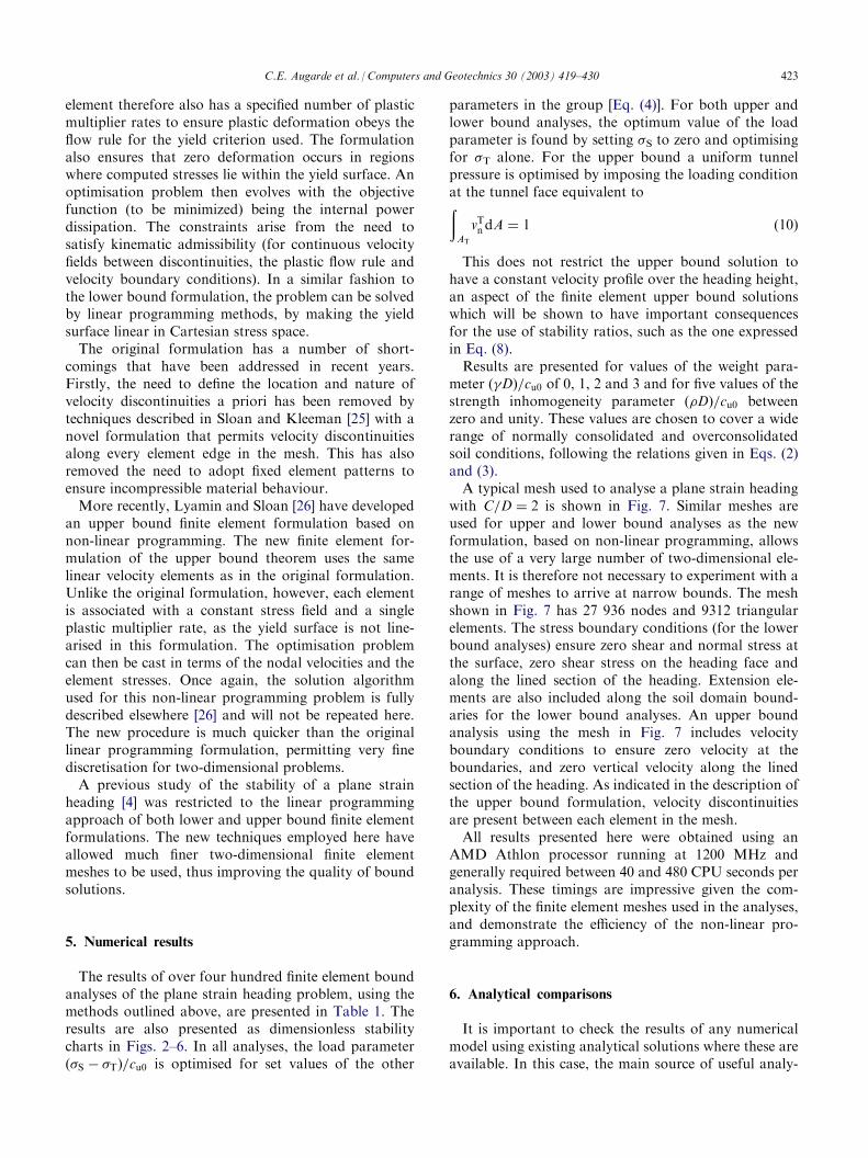
5. Numerical results

The results of over four hundred finite element boundanalyses of the plane strain heading problem, using themethods outlined above, are presented in Table 1. Theresults are also presented as dimensionless stabilitycharts in Figs. 2–6. In all analyses, the load parameter�S � �Tð Þ=cu0 is optimised for set values of the other

parameters in the group [Eq. (4)]. For both upper andlower bound analyses, the optimum value of the loadparameter is found by setting �S to zero and optimisingfor �T alone. For the upper bound a uniform tunnelpressure is optimised by imposing the loading conditionat the tunnel face equivalent toðAT

vTndA ¼ 1 ð10Þ

This does not restrict the upper bound solution tohave a constant velocity profile over the heading height,an aspect of the finite element upper bound solutionswhich will be shown to have important consequencesfor the use of stability ratios, such as the one expressedin Eq. (8).Results are presented for values of the weight para-

meter �Dð Þ=cu0 of 0, 1, 2 and 3 and for five values of thestrength inhomogeneity parameter �Dð Þ=cu0 betweenzero and unity. These values are chosen to cover a widerange of normally consolidated and overconsolidatedsoil conditions, following the relations given in Eqs. (2)and (3).A typical mesh used to analyse a plane strain heading

with C=D ¼ 2 is shown in Fig. 7. Similar meshes areused for upper and lower bound analyses as the newformulation, based on non-linear programming, allowsthe use of a very large number of two-dimensional ele-ments. It is therefore not necessary to experiment with arange of meshes to arrive at narrow bounds. The meshshown in Fig. 7 has 27 936 nodes and 9312 triangularelements. The stress boundary conditions (for the lowerbound analyses) ensure zero shear and normal stress atthe surface, zero shear stress on the heading face andalong the lined section of the heading. Extension ele-ments are also included along the soil domain bound-aries for the lower bound analyses. An upper boundanalysis using the mesh in Fig. 7 includes velocityboundary conditions to ensure zero velocity at theboundaries, and zero vertical velocity along the linedsection of the heading. As indicated in the description ofthe upper bound formulation, velocity discontinuitiesare present between each element in the mesh.All results presented here were obtained using an

AMD Athlon processor running at 1200 MHz andgenerally required between 40 and 480 CPU seconds peranalysis. These timings are impressive given the com-plexity of the finite element meshes used in the analyses,and demonstrate the efficiency of the non-linear pro-gramming approach.

6. Analytical comparisons

It is important to check the results of any numericalmodel using existing analytical solutions where these areavailable. In this case, the main source of useful analy-


tical checks on the numerical results comes from Ref.[6]. They present analytical solutions for lower andupper bounds of the load parameter �S � �Tð Þ=cu0 forundrained soil with constant strength with depth. Forthe case of a weightless soil �Dð Þ=cu0 ¼ 0, a lower bound

can be obtained by adapting the solution for a v-not-ched bar under tension, given in [27]

�S � �Tcu0

5 2þ 2logC

Dþ 1

� ð11Þ

Table 1

Bounds on the load parameter for stability of an undrained plane strain heading

C

D

�D

cu0

�D

cu0¼ 0

�D

cu0¼ 1

�D

cu0¼ 2

�D

cu0¼ 3

Lower

bound

Upper

bound

Lower

bound

Upper

bound

Lower

bound

Upper

bound

Lower

bound

Upper

bound

1 0.00 4.00 4.39 2.46 2.89 0.85 1.39 �0.74 �0.11

1 0.25 5.32 5.59 3.82 4.09 2.29 2.59 0.68 1.09

1 0.50 6.47 6.77 4.98 5.27 3.46 3.77 1.87 2.27

1 0.75 7.60 7.93 6.12 6.43 4.62 4.93 3.04 3.43

1 1.00 8.73 9.09 7.25 7.59 5.76 6.09 4.19 4.59

2 0.00 5.05 5.68 2.40 3.18 �0.20 0.68 �2.84 �1.82

2 0.25 7.93 8.10 5.43 5.60 2.91 3.08 0.37 0.54

2 0.50 10.42 10.66 7.93 8.17 5.43 5.66 2.90 3.14

2 0.75 12.89 13.19 10.41 10.71 7.91 8.21 5.40 5.70

2 1.00 15.35 15.72 12.87 13.24 10.38 10.74 7.87 8.24

3 0.00 5.75 6.50 2.20 3.00 �1.40 �0.50 �5.03 �4.00

3 0.25 10.20 10.50 6.70 7.00 3.19 3.48 �0.35 �0.05

3 0.50 14.23 14.66 10.74 11.16 7.24 7.66 3.72 4.14

3 0.75 18.23 18.79 14.75 15.30 11.25 11.80 7.75 8.30

3 1.00 22.22 22.91 18.74 19.42 15.25 15.93 11.75 12.43

4 0.00 6.25 7.21 1.71 2.71 �2.86 �1.79 �7.49 �6.29

4 0.25 12.52 12.82 8.03 8.32 3.52 3.81 �1.01 �0.72

4 0.50 18.28 18.72 13.79 14.23 9.29 9.72 4.78 5.21

4 0.75 24.01 24.59 19.52 20.10 15.03 15.60 10.53 11.09

4 1.00 29.72 30.45 25.24 26.00 20.75 21.46 16.25 16.96

5 0.00 6.70 7.70 1.15 2.20 �4.48 �3.30 �10.11 �8.80

5 0.25 14.81 15.19 9.32 9.69 3.81 4.18 �1.71 �1.35

5 0.50 22.40 22.98 16.92 17.48 11.42 11.98 5.91 6.47

5 0.75 29.96 30.72 24.48 25.23 18.99 19.73 13.49 14.23

5 1.00 37.51 38.46 32.03 32.97 26.54 27.47 21.05 21.97

6 0.00 7.02 8.12 0.41 1.62 �6.10 �4.88 �12.90 �11.38

6 0.25 17.14 17.58 10.65 11.08 4.14 4.57 �2.39 �1.95

6 0.50 26.67 27.36 20.18 20.87 13.69 14.36 7.18 7.86

6 0.75 36.17 37.11 26.69 30.61 23.20 24.11 16.70 17.61

6 1.00 45.66 46.84 39.17 40.34 32.69 33.85 26.19 27.35

7 0.00 7.33 8.49 �0.32 0.99 �7.90 �6.51 �15.53 �14.01

7 0.25 19.47 20.02 11.98 12.50 4.47 5.00 �3.05 �2.52

7 0.50 31.01 31.87 23.53 24.37 16.03 16.87 8.53 9.36

7 0.75 42.53 43.70 35.04 36.20 27.55 28.71 20.06 21.21

7 1.00 54.02 55.51 46.54 48.02 39.06 40.53 31.56 33.03

8 0.00 7.46 8.83 �1.21 0.33 �9.80 �8.17 �18.43 �16.67

8 0.25 21.82 22.46 13.33 13.96 4.82 5.45 �3.70 �3.06

8 0.50 35.44 36.49 26.95 27.99 18.46 19.49 9.96 10.99

8 0.75 49.02 50.48 40.55 41.99 32.06 33.49 23.56 24.99

8 1.00 62.60 64.46 54.12 55.97 45.64 47.47 37.14 38.97

9 0.00 7.57 9.08 �2.16 �0.42 �11.75 �9.92 �21.39 �19.42

9 0.25 24.19 24.95 14.70 15.46 5.19 5.95 �4.33 �3.57

9 0.50 39.94 41.21 30.46 31.72 20.96 22.22 11.46 12.71

9 0.75 55.66 57.43 46.17 47.94 36.68 38.44 27.19 28.94

9 1.00 71.37 73.64 61.88 64.15 52.40 54.65 42.90 45.16

10 0.00 7.70 9.32 �3.16 �1.18 �13.75 �11.68 �24.39 �22.18

10 0.25 29.58 27.48 16.09 16.98 5.58 6.48 �4.94 �4.03

10 0.50 44.51 46.03 34.02 35.54 23.52 25.04 13.02 14.53

10 0.75 62.40 64.54 51.92 54.05 41.43 43.55 30.93 33.06

10 1.00 80.29 83.06 69.80 72.56 59.32 62.06 48.82 51.57


For the case of a soil with self-weight, �Dð Þ=cu0 6¼ 0,Davis et al. [6] suggest it is acceptable to add a hydro-static stress field to the weightless case to obtain a solu-tion. This is not a strict lower bound, as the tunnelpressure now varies linearly with depth, rather thanbeing constant over the depth; the condition used toderive the original weightless lower bound solution. If�T is taken instead to represent the mean tunnel pres-sure over the heading height then this solution can be

written

�S � �Tcu0

5 2þ 2logC

Dþ 1

� ��D

cu0

C

Dþ1

2

� ð12Þ

Davis et al. [6] suggest this is, however, a safe solutionbased on their results for the other stability problems.These lower bound solutions are by inspection, alsolower bound solutions for the case of inhomogeneoussoil, albeit very poor ones.

Fig. 2. Bounds on load parameter for �Dð Þ=cu0 ¼ 0.

Fig. 3. Bounds on load parameter for �Dð Þ=cu0 ¼ 0:25.




An analytical upper bound solution can be obtainedfrom the five variable mechanism shown in Fig. 8 [4].This is a rigid block mechanism where the internalpower dissipation takes place along the interfacesbetween blocks only. The mechanism may appear to beincompatible in that the tip of the triangle at the face ofthe heading has to penetrate the soil beneath. This dif-ficulty is dealt with by noting that if the tip deformsplastically to accommodate this movement the energydissipated is of second order to that dissipated in theinterfaces between blocks for a given movement, andcan be neglected in the analysis [28]. Similar mechan-isms are also used by Davis et al. [6]. For the case of aconstant undrained strength �Dð Þ=cu0 ¼ 0, equatingexternal and internal power dissipation and rearranginggives the following expression for the load parameter,

�S � �Tcu0

�Dcu0

¼0

¼

2C

D

sin�2sin�4sin�1sin�3sin�5cos �1 þ �2 þ �3 þ �4 þ �5ð Þ

� �

þ cot�1 þ 2cot�2 þ 2cot�3 þ 2cot�4 þ cot�5

þcos �1 þ �2 þ �3 þ �4ð Þ

sin�5cos �1 þ �2 þ �3 þ �4 þ �5ð Þ��D

cu0

C

Dþ1

2

� �ð13Þ

This mechanism can also be used for the case ofvarying soil strength with depth, in which case theexpression for the load parameter is

�S � �Tcu0

�Dcu0

6¼0

¼�S � �T

cu0

�Dcu0

¼0

þ�D

cu0

�C

D

cot�1 þ 2cot�2 þ 2cot�3 þ 2cot�4 þ cot�5

þcos �1 þ �2 þ �3 þ �4ð Þ

sin�5cos �1 þ �2 þ �3 þ �4 þ �5ð Þ

0B@

1CAþ

C

D

� 2

sin�2sin�4sin�1sin�3sin�5cos �1 þ �2 þ �3 þ �4 þ �5ð Þ

�

þ1

2sin�2

sin �1 þ �2ð Þ

sin�1� cos �1 þ �2ð Þ

cos�1þ sin�1 2cot�2þ2cot�3þcot�4ð Þð Þ

0B@

1CA

þ1

2sin�2

cos �1 þ �2 þ �3 þ �4ð Þ

sin�4sin�3 cot�4þcot�5ð Þð Þ

þsin�3cos �1 þ �2 þ �3 þ �4ð Þ

sin�5cos �1 þ �2 þ �3 þ �4 þ �5ð Þ

þsin �3 þ �4ð Þ

sin�4

0BBBBBBB@

1CCCCCCCA

�

ð14Þ


Fig. 7. Typical finite element mesh for C/D=2.


Upper bounds can then be found by numericallyoptimising Eqs. (13) and (14). Values thus obtained areincluded, where appropriate, with the plots of the finiteelement results, in Figs. 2–6. A limited number of casesonly, for the analytical solutions given above, are inclu-ded in these figures, because the finite element resultsusually provide much better bounds and also for thesake of clarity.It is notable that upper bound solutions for soils

where �D=cu0 > 0 can be derived from the weightlesssolutions by subtraction of a term including two of thedimensionless groups.This apparently convenient result was derived inde-

pendently for any upper bound solution of this problemby Sloan and Assadi [4]. It appears to make the use of astability ratio N, as defined in Eq. (8), rather attractiveas the term deducted from the upper bound solutionsfor �D=cu0 > 0 is equal to the term added to the loadparameter to obtain N. One stability parameter there-fore covers all cases of soil with and without self-weight,for a particular configuration of heading. This isapplicable only in certain cases, however, as will bedemonstrated below.The external power term required for the upper

bound analysis [Eq. (7)] includes an integral of the verticalvelocity v of points in the soil mass. Due to the incom-pressibility of the soil it is possible to replace this integralwith a simpler term that can be evaluated in terms of thegeometry of the problem and the nature of the horizontalvelocity profile applied to the tunnel face as follows:

ðV

v dV ¼

ðCþD

C

zvTn dz ð15Þ

where vTn is the horizontal outward velocity at the faceof the heading (as before) and z is the vertical coordi-nate, as shown in Fig. 1. [A detailed proof of the deri-vation of Eq. (15) is given by Sloan and Assadi [4]]. If a

uniform outward velocity field vTn ¼ is imposed on theheading face then, using Eq. (15) the volume integral inEq. (7) isðV

v dV ¼ D CþD

2

� ð16Þ

Substituting this result into the expression for theexternal power expended [Eq. (7)] and equating to theinternal power, Pint gives

Pint ¼�S � �T

cu0

� cu0Dþ

�D

cu0

� cu0D Cþ

D

2

� ð17Þ

Hence we can write the result for soil with self-weightin terms of the solution for the weightless soil as

�S � �Tcu0

� �Dcu0

6¼0

¼�S � �T

cu0

� �Dcu0

¼0

��D

cu0

� C

Dþ1

2

� ð18Þ

This is similar in form to the upper bound solutionsusing the rigid block mechanism in Fig. 8 [Eqs. (13) and(14)]. As is now evident, however, the second term inEq. (18) changes according to the chosen velocity dis-tribution on the heading face. If, for example, the velo-city vTn varies linearly from at the top of the heading tozero at the base, as shown in Fig. 9, the second term on

the right hand side of Eq. (18) becomes�D

cu0

� C

Dþ1

3

� .

7. Discussion

The numerical results presented in Figs. 2–6 showvery close bounds on the load parameter �S � �Tð Þ=cu0for a wide range of problem configurations. The close-ness of the bounds, and the feasibility of conductingsuch a large study, can be attributed to the improve-

Fig. 8. 5-variable rigid block mechanism for analytical upper bound.

Fig. 9. Linear variation of velocity over heading depth.


ments in the algorithms used to solve the non-linearprogramming problem, resulting from the finite elementbound formulation. In the majority of cases the boundsolutions bracket the real solution to within 4%. Asthe soil weight parameter �D=cu0 is increased, the gapbetween the bounds widens slightly, as does the calcu-lation time to obtain the results.A negative value of the load parameter �S � �Tð Þ=cu0

indicates the heading configuration is inherentlyunstable; i.e. a positive heading pressure is required toprevent collapse, with zero surcharge. This situationoccurs for a limited range of headings, generally forheavy soils, with �Dð Þ=cu0 5 2 where there is little or noincrease of strength with depth. For all cases wherethere is appreciable inhomogeneity[with �Dð Þ=cu0 5 0:5], all headings are stable for zerosurcharge and zero heading pressure.The analytical and rigid-block bound solutions [Eqs.

(11)–(14)] improve on the finite element results for onecase only (C=D ¼ 2; �D=cu0 ¼ �D=cu0 ¼ 0) and ingeneral provide much poorer solutions. For shallowheadings with low soil weight, however, the analyticalupper bound solutions [Eqs. (13) and (14)] are very closeto those given by the finite element methods. The lowerbound solution for soils with self-weight, suggested byDavis et al. [6] are indeed safe, as can be seen in Fig. 2.This solution also appears to follow the same trend asthe finite element lower bound solutions.Another noticeable feature of the results is the relative

importance of soil weight and strength profile. As thelatter is increased from 0.5 to unity, the importance ofthe soil weight profile decreases considerably. When�Dð Þ=cu0 ¼ 0:5, the load parameter is reduced three-foldas the weight parameter changes from zero to 3. For thesteepest increase in strength with depth �Dð Þ=cu0 ¼ 1:0,

the load parameter for weightless soils conditions isonly 1.6 times that at the highest weight parameter. Theopposite effect happens when the heading is located at agreater depth. Fig. 10 shows the variations in the loadparameter as weight increases, from C=D ¼ 1 toC=D ¼ 3. The plots for the shallow heading are closelyspaced, in contrast to those for the deeper heading. Thisconfirms, perhaps obviously, that the determination ofthe variable � assumes greater importance as the head-ing depth increases.Fig. 10 also shows a linear variation in load para-

meter with weight parameter, for both upper and lowerbound results. This follows the predictions from theanalytical upper bound solutions discussed above,where solutions for soils with self-weight are found bysubtracting a term dependent on �D=cu0 from theweightless load parameter.Fig. 11a shows the velocity vectors at nodes in an

upper bound mesh for a heading whereC=D ¼ 1; �D=cu0 ¼ 3; �D=cu0 ¼ 0. Horizontalcomponents at the tunnel face (i.e. values of vTn ) areclearly non-uniform over the tunnel height. In this case,therefore, the stability number given in Eq. (8) wouldnot be valid. This demonstrates that the safe use of astability number, N, requires prior knowledge of thevelocity profile over the heading height. Similar conclu-sions may be drawn for other underground stabilityproblems in geomechanics. Non-uniform horizontalvelocity profiles at the heading face, obtained in thefinite element solutions, are shown to produce betterupper bound solutions and to invalidate the use of thestability ratio as described by Eq. (8). There are alsointeresting differences in the patterns of these velocitiesas soil weight increases and as headings are deepened.The effect of increasing soil weight is to make the velo-

Fig. 10. Load parameters replotted for varying weight parameter.


city profile over the heading depth less uniform. Fig. 11bshows the profile for C=D ¼ 1; �D=cu0 ¼0; �D=cu0 ¼ 0 and indicates relatively uniform velo-city vectors over the heading depth. Fig 10a, in contrastshows the velocity vectors for the same analysis with�D=cu0 ¼ 3. The profile, as highlighted above, is clearlyless uniform with greater velocities to the base of theheading and reduced velocities at the top. This patternis evident for all depths of heading studied here. Fig. 12aand b show a similar effect for the case where C=D ¼ 5.Clearly, increased soil weight leads to a larger variationin vertical stress across the heading and this may lead toearlier yield and a greater contribution to continuumplastic flow in the base of the heading. Fig. 12 alsoshows the finite element upper bound to depart from therigid block mechanism of Fig. 8 once the heading is atdepth. Non-zero velocities are predicted for nodesabove the lined section of the tunnel for this case,C=D ¼ 5, and deeper cases. For the case of C=D ¼ 1,velocity discontinuities appears to line up verticallyfrom the top of the heading, similar to the rigid blockmechanism of Fig. 8.

8. Conclusion

The stability of a plane strain heading in undrainedconditions has been investigated using finite elementbound methods. Improvements to solution algorithmshave permitted very close bounds to be drawn in mostcases, providing useful charts for those assessing the sta-bility of this type of underground opening. It is impor-tant to remember that, in practice, the drained stabilityshould also be considered, an area not covered in thispaper. The use of a universal stability ratio [19] has beenshown not to be advisable, depending as it does on thenature of collapse which cannot be determined a priori.

Fig. 11. Velocity vectors for finite element upper bound analyses

C=D ¼ 1; �D=cu0 ¼ 0: (a) �D=cu0 ¼ 0, (b) �D=cu0 ¼ 3.

Fig. 12. Velocity vectors for finite element upper bound analyses

C=D ¼ 5; �D=cu0 ¼ 0: (a) �D=cu0 ¼ 0, (b) �D=cu0 ¼ 3.


Acknowledgements

The work presented in this paper was carried outwhile the first author was visiting the University ofNewcastle, Australia. During this period he was sup-ported by an IREX Fellowship, awarded by the Aus-tralian Research Council.

References

[1] Salencon J. An introduction to the yield design theory and its

application to soil mechanics. European Journal of Mechanics A/

Solids 1990;9(5):477–500.

[2] Lysmer J. Limit analysis of plane problems in soil mechanics.

ASCE Journal of the Soil Mechanics and Foundations Division

1970;96(SM4):1311–34.

[3] Anderheggen E, Knopfel H. Finite element limit analysis using

linear programming. International Journal of Solids and Struc-

tures 1972;8:1413–31.

[4] Sloan SW, Assadi A. Undrained stability of a plane strain head-

ing. Canadian Geotechnical Journal 1994;31:443–50.

[5] Mair, RJ. Centrifugal modelling of tunnel construction in soft

clay. PhD thesis, University of Cambridge, 1979.

[6] Davis EH, Gunn MJ, Mair RJ, Seneviratne HN. The stability of

shallow tunnels and underground openings in cohesive material.

Geotechnique 1980;30:397–416.

[7] Muhlhaus H-B. Lower bound solutions for tunnels in two and

three dimensions. Rock Mechanics and Rock Engineering 1985;

18:37–52.

[8] Atkinson JH, Potts DM. Stability of a shallow circular tunnel in

cohesionless soil. Geotechnique 1977;27:203–15.

[9] Leca E, Dormieux L. Upper and lower bound solutions for the

face stability of shallow circular tunnels in frictional material.


[10] Eisenstein Z, Samarasekara L. Stability of unsupported tunnels

in clay. Canadian Geotechnical Journal 1992;29:609–13.

[11] Anagnostou G, Kovari K. Face stability conditions with earth-

pressure-balanced shields. Tunnelling and Underground Space

Technology 1996;11:165–73.

[12] Sloan SW, Assadi A. Undrained stability of a square tunnel

whose strength increases linearly with depth. Computers and

Geotechnics 1991;12:321–46.

[13] Sloan SW, Assadi A. The stability of tunnels in soft ground. In:

Houlsby GT, Schofield AN, editors. Predictive soil mechanics.

London: Thomas Telford 1993, p. 644–63.

[14] Lyamin AV, Sloan SW. Stability of a plane strain circular tunnel

in a cohesive-frictional soil. In: Proceedings of the J.R. Booker

Memorial Symposium, Sydney, 2000. p. 139–53.

[15] Skempton AW. The planning and design of the new Hong Kong

airport. Discussion. Proc Inst Civil Eng 1957;7:305–7.

[16] Atkinson JH, Bransby PL. The mechanics of soils: an intro-

duction to critical state soil mechanics. London: McGraw-Hill;

1978.

[17] Ladd CC, Foote R., Ishihara K, Schlosser F, Poulos HG. Stress

deformation and strength characteristics. In: Proc. 12th Int.

Conf. Soil Mechanics and Foundation Engineering, Vol. 2, 1977.

p. 421–94.

[18] Butterfield R. Dimensional analysis for geotechnical engineers.


[19] Broms BB, Bennermark H. Stability of clay in vertical openings.

Journal of the Geotechnical Engineering Division, ASCE 1967;

193:71–94.

[20] Atkinson JH, Mair RJ. Soil mechanics aspects of soft ground

tunnelling. Ground Engineering 1981;14:20–4.

[21] Sloan SW. Lower bound limit analysis using finite elements and

linear programming. International Journal for Numerical and

Analytical Methods in Geomechanics 1988;12:61–77.

[22] Lyamin AV. Three-dimensional lower bound limit analysis using

non-linear programming. PhD thesis, Department of Civil, Sur-

veying and Environmental Engineering, University of Newcastle,

Australia, 1999.

[23] Lyamin AV, Sloan SW. Lower bound limit analysis using non-

linear programming. International Journal for Numerical Meth-

ods in Engineering 2002;55:573–611.

[24] Sloan SW. Upper bound limit analysis using finite elements and



[25] Sloan SW, Kleeman PW. Upper bound limit analysis with dis-

continuous velocity fields. Computer Methods in Applied

Mechanics and Engineering 1995;127:293–314.

[26] Lyamin AV, Sloan SW. Upper bound limit analysis using non-



[27] Ewing DJF, Hill R. The plastic constraint of V-notched tension

bars. Journal Mech Phys Solids 1967;15:115–24.

[28] Chen WH. Limit analysis and soil plasticity. Amsterdam:

Elsevier; 1975.


Documents

Stabilityofanundrainedplanestrainheadingrevisited · Stabilityofanundrainedplanestrainheadingrevisited CharlesE.Augardea,*,AndreiV.Lyaminb,ScottW.Sloanb ... Anagnostou and Kovari