Embed Size (px)
Citation preview

Stability of Plane Couette Flow
and Pipe Poiseuille Flow
PER-OLOV ÅSÉN
Doctoral ThesisStockholm, Sweden, 2007

TRITA-CSC-A 2007:7ISSN 1653-5723ISRN KTH/CSC/A--07/07--SEISBN 978-91-7178-651-7
CSC Skolan för datavetenskap och kommunikationSE-100 44 Stockholm
SWEDEN
Akademisk avhandling som med tillstånd av Kungl Tekniska högskolan framläggestill offentlig granskning för avläggande av teknologie doktorsexamen fredagen den25 maj 2007 kl 10.15 i D3, Huvudbyggnaden, Kungl Tekniska högskolan, Lindsted-tsvägen 3, Stockholm.
c© Per-Olov Åsén, May 2007
Tryck: Universitetsservice US AB

iii
Abstract
This thesis concerns the stability of plane Couette flow and pipe Poiseuille flow in
three space dimensions. The mathematical model for both flows is the incompressible
Navier–Stokes equations. Both analytical and numerical techniques are used.
We present new results for the resolvent corresponding to both flows. For plane Cou-
ette flow, analytical bounds on the resolvent have previously been derived in parts of the
unstable half-plane. In the remaining part, only bounds based on numerical computations
in an infinite parameter domain are available. Due to the need for truncation of this
infinite parameter domain, these results are mathematically insufficient.
We obtain a new analytical bound on the resolvent at s = 0 in all but a compact
subset of the parameter domain. This is done by deriving approximate solutions of the
Orr–Sommerfeld equation and bounding the errors made by the approximations. In the
remaining compact set, we use standard numerical techniques to obtain a bound. Hence,
this part of the proof is not rigorous in the mathematical sense.
In the thesis, we present a way of making also the numerical part of the proof rigorous.
By using analytical techniques, we reduce the remaining compact subset of the parameter
domain to a finite set of parameter values. In this set, we need to compute bounds on
the solution of a boundary value problem. By using a validated numerical method, such
bounds can be obtained. In the thesis, we investigate a validated numerical method for
enclosing the solutions of boundary value problems.
For pipe Poiseuille flow, only numerical bounds on the resolvent have previously been
derived. We present analytical bounds in parts of the unstable half-plane. Also, we derive
a bound on the resolvent for certain perturbations. Especially, the bound is valid for the
perturbation which numerical computations indicate to be the perturbation which exhibits
largest transient growth. The bound is valid in the entire unstable half-plane.
We also investigate the stability of pipe Poiseuille flow by direct numerical simulations.
Especially, we consider a disturbance which experiments have shown is efficient in trigger-
ing turbulence. The disturbance is in the form of blowing and suction in two small holes.
Our results show the formation of hairpin vortices shortly after the disturbance. Initially,
the hairpins form a localized packet of hairpins as they are advected downstream. After
approximately 10 pipe diameters from the disturbance origin, the flow becomes severely
disordered. Our results show good agreement with the experimental results.
In order to perform direct numerical simulations of disturbances which are highly
localized in space, parallel computers must be used. Also, direct numerical simulations
require the use of numerical methods of high order of accuracy. Many such methods have
a global data dependency, making parallelization difficult. In this thesis, we also present
the process of parallelizing a code for direct numerical simulations of pipe Poiseuille flow
for a distributed memory computer.


Preface
This thesis contains five papers and an introduction.Paper I: Per-Olov Åsén and Gunilla Kreiss, A Rigorous Resolvent Estimate
for Plane Couette Flow, J. Math. Fluid Mech., accepted 2005. Published online.DOI:10.1007/s00021-005-0194-2.
The author of this thesis contributed to the ideas, performed the numericalcomputations and wrote the manuscript.
This paper is also part of the licentiate thesis [1].Paper II: Malin Siklosi and Per-Olov Åsén, On a Computer-Assisted Method
for Proving Existence of Solutions of Boundary Value Problems , Technical Report,TRITA-NA 0426, NADA, KTH, 2004.
The theoretical derivations were done in close cooperation between the authors,both of them contributing in an equal amount. The author of this thesis had themain responsibility for the computer implementations and wrote section 5 in thereport. Malin Siklosi had the main responsibility for the literature studies andwrote sections 1-4 in the report.
This paper is also part of the licentiate thesis [1].Paper III: Per-Olov Åsén and Gunilla Kreiss, Resolvent Bounds for Pipe
Poiseuille Flow, J. Fluid Mech., 568:451–471,2006.The author of this thesis contributed to the ideas, performed the mathematical
derivations and wrote the manuscript.Paper IV: Per-Olov Åsén, A Parallel Code for Direct Numerical Simulations
of Pipe Poiseuille Flow, Technical Report, TRITA-CSC-NA 2007:2, CSC, KTH,2007.
Paper V: Per-Olov Åsén, Gunilla Kreiss and Dietmar Rempfer, Direct Numer-ical Simulations of Localized Disturbances in Pipe Poiseuille Flow, submitted toTheoret. Comput. Fluid Dynamics 2007.
The author of this thesis contributed to the ideas, performed the simulationsand wrote the manuscript.
v


Acknowledgments
First and foremost, I would like to thank my advisor Professor Gunilla Kreiss, forher guidance, support and encouragement throughout my work at KTH, makingthe completion of this thesis possible. It has been a privilege and pleasure beingher student.
The second paper of this thesis was done in collaboration with Dr. Malin Siklosi,and I thank her for the rewarding experience of working with her.
The third paper of this thesis was partly done while visiting Professor PeterSchmid at the University of Washington, Seattle. I thank him for the stimulatingexperience of working with him.
I would like to thank the people at the department of mechanics and the Linnéflow centre. Especially, Professor Dan Henningson, Dr. Luca Brandt and Dr.Philipp Schlatter provided invaluable help on the fifth paper of this thesis.
Paper 5 would not have been possible without the excellent serial code developedby Professor Dietmar Rempfer and Dr. Jörg Reuter and I am grateful for havingbeen able to work with and develop this code. Also, the computations in the paperwere inspired from experiments by Professor Tom Mullin and Dr. Jorge Peixinhoand I thank them for fruitful conversations.
The Swedish National Infrastructure for Computing provided computer timeand the Center for Parallel Computers at KTH provided support during computa-tions and development, all of which I am grateful for. Especially, I would like tothank Dr. Ulf Andersson for helping in the parallelization of the code.
I would like to thank all present and former colleagues at CSC for providing astimulating environment to work in.
Finally, I would like to thank my family for help and support throughout theyears.
Financial support has been provided by Vetenskapsrådet and is gratefully ac-knowledged.
vii


Contents
Contents ix
1 Introduction 1
2 The Navier–Stokes Equations 3
2.1 Wall bounded shear flows . . . . . . . . . . . . . . . . . . . . . . . . 3
3 Stability of shear flows 7
3.1 Stability by resolvent analysis . . . . . . . . . . . . . . . . . . . . . . 93.2 Direct numerical simulations . . . . . . . . . . . . . . . . . . . . . . 14
4 Computer-Assisted Proofs 17
4.1 Basic Ideas . . . . . . . . . . . . . . . . . . . . . . . . . . . . . . . . 174.2 Relation to Paper 1 . . . . . . . . . . . . . . . . . . . . . . . . . . . . 19
5 Summary of Papers 23
5.1 Paper I: A Rigorous Resolvent Estimate for Plane Couette Flow . . 235.2 Paper II: On a Computer-Assisted Method for Proving Existence of
Solutions of Boundary Value Problems . . . . . . . . . . . . . . . . . 235.3 Paper III: Resolvent Bounds for Pipe Poiseuille Flow . . . . . . . . . 245.4 Paper IV: A Parallel Code for Direct Numerical Simulations of Pipe
Poiseuille Flow . . . . . . . . . . . . . . . . . . . . . . . . . . . . . . 245.5 Paper V: Direct Numerical Simulations of Localized Disturbances in
Pipe Poiseuille Flow. . . . . . . . . . . . . . . . . . . . . . . . . . . . 24
Bibliography 27
ix


Chapter 1
Introduction
The main topic of this thesis is the stability of incompressible plane Couette flowand pipe Poiseuille flow. Plane Couette flow is the stationary flow between twoinfinite parallel plates, moving in opposite directions at a constant speed, and pipePoiseuille flow is the stationary flow in an infinite circular pipe, driven by a constantpressure gradient in the axial direction. The mathematical model describing bothflows is the Navier–Stokes equations. The reason for studying these flows is thatthey are simple examples of shear flows and the steady analytical solution is knownin both cases. A better understanding of the stability of plane Couette flow andpipe Poiseuille flow could provide information useful for more complicated flows.Inducing or avoiding turbulence by active or passive control would have significantimpact in various areas. For example, when mixing fuel and air in an engine, a highlevel of turbulence intensity is desired for an efficient mixing. The air flow arounda moving car or airplane is turbulent in large regions which results in high skinfriction. By reducing the areas where the flow is turbulent, lower fuel consumptioncould be achieved. Which mechanisms are important in the transition to turbulenceis not understood. A further insight in this area is crucial for controlling turbulence.
Paper 1 concerns the stability of plane Couette flow by bounding the normof the resolvent at the point s = 0 in the unstable half-plane. Previously derivedbounds have been based on numerical computations in parts of an infinite parameterdomain. We present new analytical results for the resolvent. These results imply asharp bound on the resolvent in all but a compact subset of the infinite parameterdomain. By reducing the domain where computations are needed to a compactset, it is possible to derive a mathematically rigorous bound by using a validatednumerical method. This is the topic of paper 2, where we evaluate a method forproving existence and enclosures of solutions of boundary value problems by usingnumerical computations. Hence, paper 2 provides a way of making the bound onthe resolvent in paper 1 rigorous.
Papers 3 − 5 concern the stability of pipe Poiseuille flow. In paper 3, resolventbounds are derived in parts of the unstable half-plane. The remaining domain
1

2 CHAPTER 1. INTRODUCTION
grows with the Reynolds number. We also derive resolvent bounds for perturbationssatisfying certain conditions. These bounds are valid in the entire unstable half-plane. No numerical computations are used in paper 3. In order to analyze thestability of pipe Poiseuille flow in detail, direct numerical simulations (DNS) canbe used. Even in simple geometries like a pipe, such computations require theuse of massive computing resources. The use of high order methods in codes forDNS can make parallelization difficult. This is the topic of paper 4, in which wedescribe the parallelization of a DNS code for pipe Poiseuille flow and show resultsof good parallel performance. In paper 5, results from the parallel DNS code arepresented. Especially, we consider a spatially highly localized disturbance which inexperiments have shown to be efficient in triggering turbulence.
The initial chapters in the thesis give a brief background to the topics of the fivepapers. In chapter 2, the Navier–Stokes equations are introduced, and some previ-ous results are presented. The literature available on the Navier–Stokes equationsis vast, and some references to books are given for further reading. Also, some clas-sical cases of wall bounded shear flows are introduced in this chapter. In chapter3, the stability of flows are discussed, with emphasis on the two shear flows con-sidered in this thesis. Some previous results are presented, both of experimentaland mathematical type. Special attention is given to the methods for analyzingstability considered in this thesis. In chapter 4, the use of numerical, approximatesolutions for mathematical proofs is discussed. The idea of using computers formathematically rigorous proofs is almost a contradiction. The inherent roundingerrors in floating-point calculations and the necessity of finite dimensional modelsin a computer seem impossible to overcome. We give the basic ideas of how theseobstacles can be conquered by using well known results from functional analysisand by using a different representation of real numbers when stored in a computer.The ideas are focused on the method implemented in paper 2. We also describe indetail how the method in paper 2 can be used to make the numerical part of theproof in paper 1 rigorous. Chapter 5 contains short summaries of the five papersin the thesis. The summaries are slightly more extensive than the correspondingabstracts and are included for the readers convenience.

Chapter 2
The Navier–Stokes Equations
A mathematical description of the flow of a viscous incompressible fluid was firstderived in the early 19th century by Navier. Shortly after, others gave the equationsa more firm mathematical foundation. The result was the widely known Navier–Stokes equations.
Given a domain Ω ⊂ Rn, let u(t, x) = (u1(t, x), . . . , un(t, x)) be the velocity
and p(t, x) the pressure at (t, x) = (t, x1, . . . , xn). The non-dimensionalized Navier–Stokes equations give the evolution of the flow as
ut + (u · ∇)u + ∇p =1
R∆u,
(2.1)∇ · u = 0.
Here, R is the Reynolds number given by R = V L/ν, where V and L are typicalvelocity and length scales, respectively, and ν is the kinematic viscosity of the fluid.The equations must also be supplemented with initial and boundary conditions.
It is well known that in two space dimensions, (2.1) has a unique solution forall times under some restrictions on the initial condition. In three space dimen-sions, there are local (in time) existence results which can be extended to globalexistence results if the initial condition is small enough in some suitable norm, seee. g. [44] p. 345. Since the analytical solution of (2.1) is only known in a few specialcases, obtaining the solution usually involves the use of some numerical method.Existence and uniqueness results are then valuable. For further reading about themathematical properties of the Navier–Stokes equations, we refer to [14, 44, 54].
2.1 Wall bounded shear flows
In shear flows, the fluid motion is dominated by sheets of fluid moving in differentvelocities parallel to each other. Although seemingly a substantial simplification,shear flows are present in more complicated flows when considering the flow suffi-ciently close to an object. In this section, we describe three classical wall bounded
3

4 CHAPTER 2. THE NAVIER–STOKES EQUATIONS
shear flows which have been studied extensively; the main reason for their achievedpopularity being that they all are analytical solutions of the Navier–Stokes equa-tions.
All three flows concern the flow in simple geometries. Pipe Poiseuille flow, alsoknown as Hagen–Poiseuille flow, is the (incompressible) flow in an infinite pipe ofconstant radius. The flow is driven by a constant non-zero pressure gradient in theaxial direction. The other two classical wall bounded shear flows are plane Couetteflow and plane Poiseuille flow. Both flows concern the flow between two infiniteparallel plates. In plane Couette flow, the plates are moving in opposite directionsat a constant speed and in plane Poiseuille flow, the plates are stationary and theflow is driven as in pipe Poiseuille flow, i. e. by a constant non-zero pressure gradientin the streamwise direction.
The stationary solutions of these flows are parallel flows, where the velocityonly depends on the distance from the wall; for plane Couette flow, the solution isa velocity profile which varies linearly between the velocities of the two plates andin plane and pipe Poiseuille flow, the solution is a parabolic velocity profile in thedirection of the negative pressure gradient, see Figure 2.1.
Figure 2.1: Stationary solution of plane Couette flow (left) and plane and pipePoiseuille flow (right)
The length scale used in the definition of the Reynolds number is in pipe flowthe diameter of the pipe and in the channel flows half the distance between theplates. The velocity scale used is half the velocity difference between the platesin plane Couette flow and the maximum and mean velocity in plane and pipePoiseuille flow, respectively. For the channel, the coordinate system is chosen suchthat x1 is the streamwise direction, x2 the direction normal to the plates and x3
the spanwise direction. The plates are located at x2 = ±1, i. e. the domain isΩc = x ∈ R
3| − 1 ≤ x2 ≤ 1. In the case of pipe Poiseuille flow, cylindricalcoordinates, (r, φ, z), are used and the pipe radius is one, yielding the domainΩp = (r, φ, z)|0 ≤ r ≤ 1, 0 ≤ φ ≤ 2π, z ∈ R. The stationary solutions are now

2.1. WALL BOUNDED SHEAR FLOWS 5
given by
U =
x2ex1, for plane Couette flow,
(1 − x22)ex1
, for plane Poiseuille flow,(1 − r2)ez, for pipe Poiseuille flow.
Plane Couette flow, plane Poiseuille flow and pipe Poiseuille flow have been ex-tensively studied by applied mathematicians throughout the years, mainly becausethey are some of the simplest examples of flows available. However, despite theirsimplicity much is still unknown about the effects of perturbations on the stationaryflows. A better understanding of the important mechanisms in these flows couldhave implications for other, more complicated, flows.


Chapter 3
Stability of shear flows
The field of hydrodynamic stability concerns the stability of various flows whensubjected to disturbances. This is an important concept since a stationary unstableflow can not exist in reality. Also, a flow can be stable to some disturbances whileunstable to others. A disturbance generating a perturbation which grows with timemight lead to turbulence. Quantifying for which disturbances a flow is stable is ofgreat importance in various applications. For an introduction to the field, we referto the books [8, 9, 41].
Given a flow U , P which solves (2.1), the effect of a disturbance, u0, can beinvestigated by considering the equations for the perturbed state. Let the deviationfrom the given flow be denoted by u, p. Since both the given flow U , P and theperturbed state U + u, P + p satisfy (2.1), subtracting the equations yields
ut + (u · ∇)u + (U · ∇)u + (u · ∇)U + ∇p =1
R∆u,
(3.1)∇ · u = 0,
with initial condition u(x, 0) = u0.In order to define stability, we need a norm to measure the size of the perturb-
ation. The most commonly used norm is the L2-norm, since it corresponds to thekinetic energy of the perturbation. However, any norm can be used and in somecases other choices of norms might be more suitable.
The flow U is called stable to the disturbance u0 if the norm of the resultingperturbation becomes arbitrarily small as time increases, i. e. if
limt→∞
‖u(t)‖ = 0. (3.2)
If the flow is stable to all disturbances, it is called globally stable. Usually, the flowis only stable to all disturbances which are small enough, i. e. to all disturbancessatisfying ‖u0‖ < γ for some γ > 0. This is known as conditional stability.
The type of stability a flow exhibits typically depends on the Reynolds number,R. At low R, the flow might be globally stable, while being conditionally stable at
7

8 CHAPTER 3. STABILITY OF SHEAR FLOWS
higher R. Especially, some flows have a critical Reynolds number, RC , such thatfor R > RC , the flow is not conditionally stable. This means that there exists atleast one infinitesimal disturbance such that the flow is not stable. Determininghow the stability depends on the Reynolds number for different flows is of centralinterest in hydrodynamic stability.
Substantial insight in the stability properties of a flow can be obtained by exper-imental investigations. Numerous experiments have been performed over the years,both for plane Couette flow and pipe Poiseuille flow. Osborne Reynolds made ex-tensive experimental investigations of pipe flow in the late 19th century; the mainachievement of the experiments was the discovery that one non-dimensional num-ber, subsequently named after him, characterized the stability of the flow. He alsonoted that for Reynolds numbers below R ≈ 2000, pipe flow is globally stable.This value has in modern experiments been estimated to R ≈ 1800 [30]. Althoughtransition to turbulence may occur at higher Reynolds numbers, laminar flow canbe maintained by avoiding disturbances. In highly controlled experiments, laminarpipe flow has been observed at R ≈ 105 [31]. The highest Reynolds number forwhich plane Couette flow is globally stable has been determined in experiments toR ≈ 350 [45].
From a mathematical point of view, the stability properties of a flow can be in-vestigated in several different ways. The most straightforward way is to consider theeigenvalues of the linearized equations, i. e. of the equations (3.1) without the non-linear term. If there exists an eigenvalue with positive real part, perturbations witha non-zero component in the direction of the corresponding eigenfunction will ex-hibit exponential growth. Determining the smallest Reynolds number which allowsexponentially growing perturbations gives the critical Reynolds number, RC . How-ever, this does not imply that for subcritical Reynolds numbers, i. e. for R < RC ,the flow is stable to all perturbations, since the effect of the nonlinear term is ig-nored. Hence, the eigenvalues give no information about the possible conditionalstability at lower Reynolds numbers.
An example of a flow with a critical Reynolds number is plane Poiseuille flow,which becomes linearly unstable at RC ≈ 5772 when the so called Tollmien–Schlichting wave becomes linearly unstable [28]. However, turbulence typicallyappears at much lower Reynolds numbers in reality. Also, the perturbation whichrequires the smallest amplitude for transition to turbulence at subcritical Reynoldsnumbers is not the Tollmien–Schlichting wave [35]. Hence, the spectrum gives poorinformation about the influence of different perturbations.
Even more misleading are the eigenvalues in the cases of plane Couette flowand pipe Poiseuille flow. Romanov proved in 1973 that plane Couette flow is lin-early stable at all Reynolds numbers [38]. In experiments however, turbulencehas been observed at Reynolds numbers as low as R ≈ 350. Pipe Poiseuille flowis believed to be linearly stable at all Reynolds numbers, although formal proofshave only been derived for axisymmetric perturbations [11] as well as for certainnon-axisymmetric perturbations [3]. In addition to these proofs, many numericalcomputations have been made indicating linear stability of pipe Poiseuille flow, see

3.1. STABILITY BY RESOLVENT ANALYSIS 9
e. g. [16, 22, 40]. Despite this linear stability, turbulence may still be observed inpipe flow for Reynolds numbers above R ≈ 1800 [30] and is the typical state athigh Reynolds numbers.
In the last two decades, the failure of eigenvalues to predict the stability ofthese flows has been explained by a phenomenon commonly referred to as transientgrowth, see e. g. [48] and the review article [39]. If all eigenvalues of the linearizedequations have negative real part, linear theory predicts that all perturbations willeventually decay exponentially. However, linear effects may still cause considerableinitial growth of a perturbation. This is due to non-orthogonality (in the consideredscalar product) of the eigenfunctions of the linearized Navier–Stokes operator. In-formation about this transient growth is not captured by the eigenvalues but canbe obtained by considering the resolvent or the ε-pseudospectrum. This is the topicof section 3.1.
Since both plane Couette flow and pipe Poiseuille flow are linearly stable, nonlin-ear effects are necessary for transition to turbulence. Computers are now powerfulenough to simulate flows in simple geometries using direct numerical simulations(DNS). The possibility of high control of disturbances and detailed analysis of res-ults makes DNS a powerful tool. Simulations can reveal which mechanisms are themost important during transition to turbulence. Such information is useful in con-trol of turbulence. An improved ability to avoid or induce turbulence would havenumerous applications; an efficient mixing of air and fuel in an engine is achievedwith a high intensity of turbulence while airplanes would reduce fuel consumption ifturbulence could be avoided. In section 3.2, direct numerical simulation is discussedfurther.
3.1 Stability by resolvent analysis
In order to analytically derive conditions for stability, the resolvent can be used. Theresolvent is the solution operator of the Laplace transformed linearized problem.Assume that we have a bound on the norm of the resolvent in the entire unstablehalf-plane. Then it is possible to derive a bound on the solution of the forcedlinear problem. This bound is given in terms of the bound on the resolvent and thenorm of the forcing. The linear bound is then extended to the nonlinear problemby treating the nonlinear term in the equation as part of the forcing. This is onlypossible if the forcing is sufficiently small. This condition gives a sufficient conditionon the size of the perturbation under which nonlinear stability is guaranteed.
We first illustrate this method on a simple model problem, similar to the modelproblem treated in [13], before discussing results for plane Couette flow and pipePoiseuille flow. For readers who are not interested in the details, the main stepsin the proof of conditional stability of the model problem are the following: Forthe linear problem corresponding to the model problem (3.3), the resolvent bound(3.4) holds in the entire unstable half-plane Re(s) ≥ 0. Using Parseval’s identityand scalar multiplication, this resolvent bound implies the bound (3.6) for the linear

10 CHAPTER 3. STABILITY OF SHEAR FLOWS
problem. If the forcing is sufficiently small, a bound for the nonlinear problem isobtained. By doing this also for the differentiated model problem, the bound (3.11)is obtained under the condition (3.12). The bound (3.11) implies stability for thenonlinear problem, i. e. we have proved conditional stability.
Model problem
Consider the following ordinary differential equation for v = (v1, v2)T ,
vt = Lv + g(v) + f(t),(3.3)
v(0) = v0,
where
L =
(
−R−1 01 −2R−1
)
, g(v) =
(
v1v2
v21
)
.
We are interested in how the stability of this system changes when the positiveconstant R grows.
Consider first the linear, unforced case g = f = 0 with initial condition v0 =(v0
1 , v02)T . Since, with R > 0, the eigenvalues of L are negative, we know that the
solution decays exponentially for sufficiently large times. However, the short timebehavior can be significantly different. The general solution of this problem is givenby
(
v1
v2
)
= v01
(
1R
)
e−t/R + (v02 − v0
1R)
(
01
)
e−2t/R.
We see that v1 decays exponentially at all times. However, Taylor expanding v2 att = 0 shows that v2 grows linearly for t ≤ O(R). This is known as transient growth,and is due to the fact that the operator L is non-normal, i. e. the eigenvectors of Lare non-orthogonal. In fact, the eigenvectors of L are (1, R)T and (0, 1)T , i. e. theyare increasingly non-orthogonal with increasing R.
We now derive conditions for stability of the nonlinear problem. Since the re-solvent method uses the Laplace transform, we consider (3.3) with homogeneousinitial conditions. Note that (3.1) could be transformed to an equivalent homogen-eous problem by e. g. introducing u = v+e−δtu0 for some δ > 0. This would resultin a forcing involving the initial perturbation, u0, in the equations for v.
Let | · | and (·, ·) denote the l2−norm and inner product of vectors and let ‖ · ‖denote the corresponding matrix norm. The linear problem corresponding to (3.3)is, after applying the Laplace transform,
sv = Lv + f (s).
The solution operator R(s) = (sI − L)−1 is known as the resolvent. With R > 0,the eigenvalues of L are negative. Hence, the resolvent is well defined in the entire

3.1. STABILITY BY RESOLVENT ANALYSIS 11
unstable half-plane, Re(s) ≥ 0. For a normal operator, N , the norm of the resolvent,R(s) = (sI − N)−1, is given by ‖R(s)‖ = supλ∈σ(N) |s − λ|−1, where σ(N) is thespectrum of N , see e. g. [12]. However, since L is non-normal, the norm of theresolvent is larger. Straightforward calculations give the sharp bound
‖(sI − L)−1‖ ≤ CR2 (3.4)
in the entire unstable half-plane.We use this to bound the solution of the linear problem. By using Parseval’s
identity, it follows that∫ T
0
|v(t)|2dt ≤
∫
∞
0
|v(t)|2dt ≤ CR4
∫
∞
0
|f(t)|2dt.
For t ≤ T , the solution v(t) does not depend on f(t) for t > T . Hence, we can setf(t) = 0 for t > T in the above expression, yielding
∫ T
0
|v(t)|2dt ≤ CR4
∫ T
0
|f(t)|2dt. (3.5)
We also need a bound on |v(T )|. Scalar multiplication of the linear equation cor-responding to (3.3) with v gives
1
2
d
dt|v(t)|2 = (v, vt) = (v, Lv) + (v, f) ≤ C1|v|
2 +1
2(|v|2 + |f |2),
where C1 is a bound on the range of L. Integrating this from t = 0 to t = T andusing (3.5) gives
|v(T )|2 ≤ CR4
∫ T
0
|f(t)|2dt.
Hence, we have the following bound for the linear problem,
|v(T )|2 +
∫ T
0
|v(t)|2dt ≤ CLR4
∫ T
0
|f(t)|2dt. (3.6)
Now, we will treat the nonlinear term as part of the forcing. For the nonlinearterm, we have
|g(v)|2 ≤ |v|4. (3.7)
Assume that the solution of the nonlinear problem (3.3) satisfies
|v(T )|2 ≤ 4R4K,(3.8)
K = CL
∫
∞
0
|f(t)|2dt,
for all times T ∈ [0,∞). We prove this assumption by assuming that it is nottrue, thus deriving a contradiction. Since v(0) = 0, (3.8) must hold with strict
12 CHAPTER 3. STABILITY OF SHEAR FLOWS
inequality for some initial time interval. Let T0 > 0 be the smallest time such thatthere is equality in (3.8) and consider T ≤ T0. From the linear estimate (3.6) andthe bounds (3.7) and (3.8), we have
|v(T )|2 +
∫ T
0
|v(t)|2dt ≤ CLR4
∫ T
0
|f(t) + g(v)|2dt
≤ 2CLR4
∫ T
0
|f(t)|2 + |v(t)|4dt
≤ 2R4K + 8CLR8K
∫ T
0
|v(t)|2dt.
We must now assume that the forcing is sufficiently small. Assume that
1 − 8CLR8K ≥ 1
2. (3.9)
Then for T ≤ T0, we have the following bound
|v(T )|2 +1
2
∫ T
0
|v(t)|2dt ≤ 2R4K. (3.10)
Clearly, the assumption of equality in (3.8) at time T0 can not be true and (3.10)must hold for all times T ∈ [0,∞).
We also need a similar bound for |vt|. This is obtained by differentiating equa-tion (3.3) with respect to t. It is easily found that |gt|2 ≤ 3(|v|2 + |vt|2). By doingthe same derivations as above for |v|2 + |vt|2, it is found that
|v(T )|2 + |vt(T )|2 +1
2
∫ T
0
|v(t)|2 + |vt(t)|2dt ≤ ˜CR4K, (3.11)
where
K = CL
∫
∞
0
|f(t)|2 + |ft(t)|2dt.
If we assume f(t) ∈ H1([0,∞)), the right hand side of (3.11) is bounded. It followsthat v(t) ∈ H1([0,∞)), which implies limt→∞ |v(t)| = 0. Thus, we have provednonlinear stability under an assumption similar to (3.9) for K instead of K, i. e.when
∫
∞
0
|f(t)|2 + |ft(t)|2dt ≤ CR−8. (3.12)
Plane Couette flow and pipe Poiseuille flow
It has been found that the eigenfunctions of the linearized operators of plane Cou-ette flow and pipe Poiseuille flow are highly non-normal in the L2-inner product,see e. g. [36, 47] . This can cause significant transient growth, as explained in the

3.1. STABILITY BY RESOLVENT ANALYSIS 13
previous section. Therefore, the resolvent or the closely related ε-pseudospectrumhas been in focus the last twenty years. The ε-pseudospectrum of a linear op-erator, L, generalizes the concept of eigenvalues by defining s to belong to theε-pseudospectrum if ‖(sI − L)−1‖ ≥ ε−1. Hence, the ε-pseudospectrum gives in-formation of where the resolvent is large, as opposed to the spectrum which onlygive information of where the resolvent is infinite or non-existing. Computations ofthe ε-pseudospectrum for plane Couette flow and pipe Poiseuille flow can be foundin e. g. [22, 47, 48].
For plane Couette flow , the resolvent, R, has been investigated by numericaland analytical techniques. In [13], the lower bound ‖R‖ ≥ CR2 was proved for theL2-norm. Here and below, we use C to denote any constant independent of theReynolds number. Numerical computations in [13, 17] indicated this asymptoticdependence to hold in the entire unstable half-plane, i. e. ‖R‖ ≤ CR2. An analyticalbound on the L2-norm of the resolvent was derived in large parts of the unstablehalf-plane in [17], where also a new norm was introduced. Computations in [17]indicated ‖R‖ ≤ CR in the new norm. This is an optimal R-dependence since thereis an eigenvalue with real part −Re(λ) ∼ R−1 [48]. For pipe Poiseuille flow, feweranalytical results about the resolvent have been derived. Numerical computationsin [22] indicate the same dependence as for plane Couette flow, i. e. ‖R‖ ≤ CR2 forthe L2-norm.
As in the example in the previous section, a bound on the resolvent can beused to prove nonlinear stability. Using this technique, the upper bound β ≤5.25 in the threshold amplitude dependence R−β was proved for wall boundedshear flows in [13], under the assumption of the resolvent bound ‖R‖ ≤ CR2.Although this upper bound on β is not sharp, it serves as the only analytical proofof conditional stability of wall bounded shear flows. However, since the resolventbounds available both for plane Couette flow and pipe Poiseuille flow are basedon numerical computations in an infinite parameter domain, the proof is not fullyrigorous.
This is the motivation of the first paper of this thesis [4]. We present a newsharp bound on the resolvent at the believed maximum s = 0. The bound is basedon analytical estimates in all but a compact subset of the parameter domain. Inthis compact set, we use numerical computations to obtain a bound. Since the set iscompact, the numerical bound can be made rigorous by using validated numericalmethods. We explain in detail how this can be done in the next chapter. Usingthe same technique, we hope to bound the resolvent in the remaining part of theunstable half-plane in the future. Moreover, analytical bounds can provide moreprecise information about the resolvent than just the maximum in the unstablehalf-plane. Such information could be used to improve the upper bound on β, i. e.to sharpen the threshold amplitude for nonlinear stability.
The third paper of this thesis [3] concerns the resolvent of pipe Poiseuille flow.We derive analytical bounds on the resolvent in large parts of the unstable half-plane. Also, a bound valid in the entire unstable half-plane is derived for per-turbations which satisfy certain relations involving the Reynolds number and the

14 CHAPTER 3. STABILITY OF SHEAR FLOWS
wave numbers in the axial and azimuthal directions. Especially, this bound onthe resolvent is valid for the perturbation which computations indicate to be theperturbation which exhibits largest transient growth [47].
3.2 Direct numerical simulations
In order to investigate the nonlinear behavior of a flow, direct numerical simulations(DNS) can be used. DNS means that the full nonlinear Navier–Stokes equationsare solved such that all length scales are resolved. This requires large amountsof computer resources as well as numerical methods with high order of accuracy.DNS are therefore so far only possible at moderate Reynolds numbers and in simplegeometries, and should therefore not be confused with an engineering tool for real-world problems.
DNS has, however, proven to be an excellent tool in research. For example, thethreshold amplitude below which perturbations eventually decay has been examinedby DNS; using different disturbances, the threshold was found to behave as R−β,with 1 ≤ β ≤ 1.25 for plane Couette flow and 1.6 ≤ β ≤ 1.75 for plane Poiseuilleflow [13, 19, 35]. The Reynolds number below which pipe Poiseuille flow is globallystable has been verified to R ≈ 1800 by using DNS [52]. Also, DNS have yieldedimportant understanding of the mechanisms behind transition to turbulence inboundary layers, see e. g. the review article [23].
Most DNS have so far been performed in planar geometries, since Cartesiancoordinates can then be used. In pipe flow, high order methods can be used by con-sidering the equations in cylindrical coordinates. However, this introduces smallergrid-cells near the center of the pipe, requiring a smaller time step. Also, additionaldifficulties arise from the polar “singularity” in the discretization. Some DNS codeshave been developed for pipe Poiseuille flow, see e. g. [10, 18, 20, 21, 27, 29, 42, 49,56]. However, these codes are typically of rather low order of accuracy and almostexclusively written for serial computers.
In the fourth paper of this thesis [2], we present the process of parallelizing acode for DNS of pipe Poiseuille flow for a distributed memory computer. The codeis based on compact finite differences of high order of accuracy in the axial direc-tion and Fourier and Chebyshev expansions in the azimuthal and radial directions,respectively [37]. These numerical techniques are computationally efficient but in-troduce a global data dependency. This makes parallelization difficult, since thereis no way to divide the problem into smaller problems which are almost independ-ent. We present our strategy of parallelization and show results on good efficiencyof the parallel code.
The fifth paper of this thesis [5] concerns DNS of pipe Poiseuille flow. We usethe parallel code developed in paper 4 in order to simulate a disturbance which ishighly localized in space. The disturbance is a combination of suction and blowingthrough two small holes located close to each other and aligned such that theyform a 45-degree angle with the pipe axis. The motivation for the simulations is
3.2. DIRECT NUMERICAL SIMULATIONS 15
that experiments have shown that this disturbance is efficient in triggering turbu-lence. Our results show an initial formation of so called hairpin vortices, which areknown to play a central role in transition to turbulence in boundary layers [6]. Thehairpins are initially advected downstream in an ordered and localized way. Afterapproximately 10 pipe diameters, the perturbation changes from being localized toa globally disordered state. Our results show good agreement with the experiments.


Chapter 4
Computer-Assisted Proofs
The invention of the computer has had a tremendous impact on the field of appliedmathematics. Problems that were practically impossible to solve 50 years ago aresolved in fractions of a second today. However, these solutions are almost never truesolutions. A numerical solution of a problem usually suffers from errors. One sourceof error is that the mathematical model might have infinite degrees of freedom,making finite dimensional approximations necessary. Deriving explicit bounds onthe errors made by the approximations is usually difficult. Another source of erroris the rounding error. Numbers like π,
√2 can not be stored exactly in a computer.
Even for numbers that are stored exactly, floating-point arithmetic is not closed.This means that even if x and y can be stored exactly, there is no guarantee thate. g. x + y can be stored exactly, making rounding necessary.
In this chapter, we give the basic ideas of how to prove existence and enclosuresof solutions of elliptic boundary value problems. This is the topic of the secondpaper of this thesis [43]. We also explain why this topic is relevant for the firstpaper of this thesis.
4.1 Basic Ideas
In this section, we describe two methods for proving existence of solutions of ellipticboundary value problems. The first method was proposed by Nakao, and has beensuccessfully used in various applications [25, 46, 50, 51, 53]. This is the method usedin paper 2 of this thesis. The second method was proposed by Plum, and has alsoproved successful [7, 15, 32, 33, 34]. The methods are quite similar in some parts,and a combination of them has been used by Nagatou, Yamamoto and Nakao [26].
Both methods rely on an approximate, numerical solution, uh, which can bederived by any numerical method. From the approximate solution, a suitable fixed-point equation, w = T (w), for the error, w = u−uh, is derived. The idea is to provethat w = T (w) has a solution in a subset of a Banach space. The subset consists of
17

18 CHAPTER 4. COMPUTER-ASSISTED PROOFS
functions with norm smaller than an explicitly derived upper bound. This upperbound gives bounds on the magnitude of the error in the approximate solution, uh.
In order to prove the existence of a solution of the fixed-point equation, Nakaoand Plum use the well known Schauder fixed-point theorem or Banach fixed-pointtheorem. The theorems state, see e. g. [55],
Theorem 4.1.1 (Schauder fixed-point theorem). Let W be a non-empty, closed,bounded, convex subset of a Banach space X. If T : W → W is a compact operator,then there exists a w ∈ W such that w = T (w).
Theorem 4.1.2 (Banach fixed-point theorem). Let W be a non-empty, closedsubset of a complete metric space X. If T : W → W is a contraction on W , thenthere exists a unique w ∈ W such that w = T (w).
Note that Theorem 4.1.2 ensures a unique solution in W , which is not the casefor Theorem 4.1.1.
Verifying that Theorem 4.1.1 or Theorem 4.1.2 can be applied to the derivedfixed-point equation and finding a suitable subset are done in different ways in theapproaches by Nakao and Plum.
In Nakao’s method, the fixed-point equation is divided into a finite dimensionalpart and an infinite dimensional part. The finite dimensional part is rewritten usingthe linearization, Lh, of the finite dimensional projection of the given equationat the approximate solution, uh. This yields an equivalent fixed-point equationwhich is more likely to map the finite dimensional part of W into itself. Verifyingthe conditions of Theorem 4.1.1 or Theorem 4.1.2 for the finite dimensional partis done by explicitly inverting Lh. The infinite dimensional part is treated byanalytical methods, using e. g. a priori error bounds on the projection into thefinite dimensional subspace.
Plum’s method uses the linearization, L, of the infinite dimensional problem atthe approximate solution, uh. Using a lower bound on the norm of L and a boundon the norm of the residual of uh, the conditions of Theorem 4.1.1 or Theorem4.1.2 are verified by analytical and numerical techniques. The main difficulty is toderive the lower bound on the norm of L. This is obtained from the eigenvalue of Lor L∗L with smallest absolute value. Deriving an enclosure of this eigenvalue canbe done by solving related finite-dimensional matrix eigenvalue problems which issuitable for computer implementation.
In both methods, the effect of the rounding errors in computations must be ac-counted for. This can be done by using interval arithmetic [24]. Interval arithmeticrepresents real numbers as closed intervals, where the upper and lower bounds ofthe intervals are floating-point numbers. Thus, all real numbers can be represented.By defining an arithmetic for the intervals, the effect of the rounding error can berigorously accounted for in each arithmetic operation. This can be extended to allelementary functions used in computations, such that the functions take intervalsas arguments and return intervals which encloses the range of the functions overthe argument intervals.

4.2. RELATION TO PAPER 1 19
4.2 Relation to Paper 1
In the first paper of this thesis, a bound on the resolvent for plane Couette flowis derived at the point s = 0. This is done by obtaining analytical bounds in allbut a compact subset of an infinite parameter domain consisting of wave numbersin two space directions and the Reynolds number. In the remaining compact set,we use standard numerical computations for a finite set of these parameter values.However, although the subset of the parameter domain is bounded, it consists ofinfinitely many parameter values. Thus, this part of the proof is not rigorous. Inthis section, we describe how the method in paper 2 could be used to make also thenumerical part of the proof rigorous.
We first summarize the procedure of making the proof in paper 1 rigorous.There are two separate problems in obtaining a rigorous bound. First, for a givenchoice of parameter values, how is a rigorous bound on the resolvent obtained bynumerical computations? The solution to this is rather straightforward. In paper 1,the problem is reduced to solving a one-dimensional boundary value problem, com-puting quantities which depend on the solution, and showing that these quantitiesfulfill certain conditions. This can be done using the method described in paper 2.The second problem is that a rigorous resolvent bound is not only needed for onechoice of parameter values but for infinitely many parameter values. This problemis solved by analytical means, resulting in Lemma 4.2.1. In short, the lemma statesthat if a rigorous resolvent bound is derived for one choice of parameter values, thenthis bound is valid in some neighborhood of the chosen parameter values. The sizeof this neighborhood is explicitly computable. Hence, rigorous resolvent boundsneed to be derived only for a finite set of parameter values. In the rest of thissection, we describe this strategy in further detail.
In paper 1, the numerical part of the proof concerns the boundary value problem
w′′(x) − (iax + b2)w(x) = 0,
w(−1) = 1, (4.1)
w(1) = 0,
in the compact parameter domain Σ = a, b ∈ R | a ∈ [1/16, 403], b2 ∈ [0, a2/3].For every combination of a and b in Σ, we need to prove two things about thesolution of (4.1). First, we need to prove that the L2-norm of the solution isbounded. Later in this section, we show that this holds for all parameter values inΣ, see the remark after the proof of Lemma 4.2.1. Secondly, we need to prove thatthe matrix
J =
(
u′(−1) −(u∗)′(1)u′(1) −(u∗)′(−1)
)
(4.2)
is non-singular. Here, (u∗)(x) denotes the complex conjugate of u(x). The matrix
20 CHAPTER 4. COMPUTER-ASSISTED PROOFS
elements are given by
u′(−1) =
∫ 1
−1
fb(σ)w(σ)dσ, (4.3)
u′(1) =
∫ 1
−1
gb(σ)w(σ)dσ, (4.4)
where
fb(σ) =
sinh(b(σ−1))sinh(2b) , b 6= 0,
σ−12 , b = 0,
(4.5)
gb(σ) =
sinh(b(σ+1))sinh(2b) , b 6= 0,
σ+12 , b = 0.
(4.6)
Note that the matrix (4.2) is non-singular if and only if |u′(−1)| 6= |u′(1)|. Hence,for a given pair of parameters, a and b, we need to enclose the solution w(x) of(4.1) and then derive rigorous enclosures of the absolute values of the integrals(4.3) and (4.4). This can be done with the method used in the second paper of thisthesis. However, since we implemented the method in MATLAB, we were not ableto obtain rigorous bounds when a is large. Using e. g. Fortran would hopefully besufficient for covering the parameter domain we are interested in.
We are still left with the problem of having an infinite number of parametervalues in Σ. This can be handled with analytical techniques. By using informationabout how far from singular J is at a given point in Σ, we are able to prove that Jis non-singular in a neighborhood around this point. The result is summarized inthe following lemma.
Lemma 4.2.1. If for a = A and b = B, the solution W (x) of (4.1) is such thatthe matrix elements (4.3) and (4.4) satisfy
|U ′(−1)| − |U ′(1)| ≥ α (4.7)
for some α > 0, then the matrix J given by (4.2) is non-singular for all parametervalues a and b satisfying
8β(‖fB‖ + ‖gB‖) + (8β + 1)(‖fb − fB‖ + ‖gb − gB‖) <α
‖W‖, (4.8)
where f and g are given by (4.5) and (4.6) and where
β = |a − A| + |b2 − B2|.
Here, ‖ · ‖ is the L2-norm on Ω = −1 ≤ x ≤ 1.
Before proving the lemma, note that it is not obvious that the quantity on theleft hand side of (4.7) should be positive. However, numerical experiments indicate
4.2. RELATION TO PAPER 1 21
this to always be the case. Of course, if the left hand side of (4.7) would be negativefor some parameter combination, a similar lemma could be derived handling thiscase.
Proof. Consider some parameter values a and b satisfying (4.8) and denote thecorresponding solution of (4.1) by w(x). From (4.1), the difference w = w − Wsatisfies
w′′ − (iax + b2)w = (i(a − A)x + (b2 − B2))W, w(±1) = 0.
Taking the L2-inner product of this equation with w, using integration by partsand taking the real part yields
‖w′‖2 + b2‖w‖2 ≤ (|a − A| + |b2 − B2|)‖W‖‖w‖ = β‖W‖‖w‖.
Using a Poincaré inequality for w and the relation cd ≤ c2/(2µ) + d2µ/2, valid forall c, d ∈ R, µ > 0, we thus have the bound
1
2‖w′‖2 +
(
1
16+ b2
)
‖w‖2 ≤ 4β2‖W‖2. (4.9)
Now, evaluating |u′(−1)| from (4.3), using w = w + W and (4.9) gives
|u′(−1)| =
∣
∣
∣
∣
∫ 1
−1
(fB(σ) + fb(σ) − fB(σ)) (w(σ) + W (σ))dσ
∣
∣
∣
∣
≥ |U ′(−1)| − ‖fB‖‖w‖ − ‖fb − fB‖(‖w‖ + ‖W‖) (4.10)
≥ |U ′(−1)| − 8β‖fB‖‖W‖ − (8β + 1)‖fb − fB‖‖W‖.
Similarly, using (4.4) yields
|u′(1)| ≤ |U ′(1)| + 8β‖gB‖‖W‖+ (8β + 1)‖gb − gB‖‖W‖. (4.11)
By (4.7), (4.8), (4.10), and (4.11), we have |u′(−1)| − |u′(1)| > 0 and thus J isnon-singular.
Remark. We stated earlier in this section that the L2-norm of the solution of(4.1) is bounded for all a and b in Σ. Since (4.9) also holds when W is the solutionwith A and B outside Σ, we can especially chose A = B = 0. Clearly, ‖W‖ is thenbounded, and it follows from (4.9) that ‖w‖ = ‖w+W‖ is bounded in any boundedparameter domain.
Hence, Lemma 4.2.1 and the method used in paper 2 provides a possibility ofderiving a rigorous bound on the resolvent in Σ, where the bound in paper 1 is notrigorous. One needs to find a finite set of points in Σ such that J is non-singularfor these points and such that the neighborhoods, given by Lemma 4.2.1, cover Σ.
In order for Σ to be covered, we must ensure that the measures of the neigh-borhoods do not become arbitrarily small even if J is non-singular. This can only

22 CHAPTER 4. COMPUTER-ASSISTED PROOFS
happen if α in (4.7) becomes arbitrarily small somewhere in Σ. However, from(4.10) and (4.11), we know that the function γ(a, b) ≡ |u′(−1)| − |u′(1)| is continu-ous with respect to a and b. Since Σ is a compact set, γ(a, b) attains a minimum,αmin, in Σ. Hence, if J is non-singular in Σ, we can cover Σ with a finite numberof neighborhoods attained from using Lemma 4.2.1. Computations made in paper1 indicate that J is non-singular, and we believe this could be proved with theapproach described in this section.
Finally, note that when computing the quantities in (4.8), all computationsshould be rigorous, using e. g. interval arithmetic. Since ‖fB‖, ‖gB‖, ‖fb − fB‖and ‖gb − gB‖ can be derived explicitly, implementation using interval arithmeticis straightforward.

Chapter 5
Summary of Papers
5.1 Paper I: A Rigorous Resolvent Estimate for Plane
Couette Flow
In this paper, we derive a rigorous bound on the resolvent for plane Couette flowat the point s = 0. We do this analytically by finding approximate solutionsof the Orr–Sommerfeld equation while keeping track of the errors made by theapproximations. This is not possible in the entire parameter domain. However,the remaining domain is bounded, and we use numerical computations to obtain abound. Previously derived bounds at s = 0 have been based on computations inan infinite parameter domain, making rigorous results impossible. In a boundeddomain, rigorous results can be derived by the use of numerical verification methodsusing interval arithmetic.
This paper is published online in Journal of Mathematical Fluid Mechanics andis entry [4] in the bibliography.
5.2 Paper II: On a Computer-Assisted Method for Proving
Existence of Solutions of Boundary Value Problems
In paper 2, we investigate a method for proving existence of solutions of ellipticboundary value problems. The method was proposed by Nakao. We solve twoproblems using this method; a linear test problem and the one-dimensional viscousBurgers’ equation. For the first problem, the method works well. For Burgers’equation however, the computational complexity becomes too large when the vis-cosity decreases. This is not surprising, since Burgers’ equation linearized at thecorrect solution rapidly becomes close to singular when the viscosity is decreased.We therefore reformulate the problem by replacing one of the boundary conditionswith a global integral condition. This approach drastically reduces the computa-tional complexity.
This paper is a technical report and is entry [43] in the bibliography.
23
24 CHAPTER 5. SUMMARY OF PAPERS
5.3 Paper III: Resolvent Bounds for Pipe Poiseuille Flow
In paper 3, we derive an analytical bound on the resolvent of pipe Poiseuille flowin large parts of the unstable half-plane. This is done by scalar multiplying the lin-earized Navier–Stokes equations (in Cartesian coordinates) with the solution andusing integration by parts. We also consider the linearized equations in cylindricalcoordinates, Fourier transformed in axial and azimuthal directions. For certaincombinations of the wave numbers and the Reynolds number, we derive an ana-lytical bound on the resolvent of the Fourier transformed problem. In particular,this bound is valid for the perturbation which numerical computations indicate tobe the perturbation that gives largest transient growth. Our bound has the samedependence on the Reynolds number as the computations give.
This paper is published in Journal of Fluid Mechanics and is entry [3] in thebibliography.
5.4 Paper IV: A Parallel Code for Direct Numerical
Simulations of Pipe Poiseuille Flow
In this paper, we describe the process of parallelizing a serial code for direct nu-merical simulations of pipe Poiseuille flow for a distributed memory computer. Theserial code, developed by Reuter and Rempfer, uses compact finite differences of atleast eighth order of accuracy in the axial direction and Fourier and Chebyshev ex-pansions in the azimuthal and radial directions, respectively. While these methodsare attractive from a numerical point of view, they give a global data dependencywhich makes the parallelization procedure complex. In the resulting parallel code,the partitioning of the domain changes between partitioning in the axial directionand partitioning in the azimuthal direction as needed. We present results showinggood speedup of the parallel code.
This paper is a technical report and is entry [2] in the bibliography.
5.5 Paper V: Direct Numerical Simulations of Localized
Disturbances in Pipe Poiseuille Flow.
In this paper, we perform direct numerical simulations of pipe Poiseuille flow sub-jected to a disturbance which is highly localized in space. The disturbance is acombination of suction and blowing in two small holes, located such that they forma 45-degree angle with the pipe axis. We perform direct numerical simulations forthe Reynolds number R = 5000. The results show a packet of hairpin vorticestraveling downstream, each having a length of approximately one pipe radius. Theperturbation remains highly localized in space while being advected downstreamfor approximately 10 pipe diameters. Beyond that distance from the disturbanceorigin the flow becomes severely disordered.

5.5. PAPER V: DIRECT NUMERICAL SIMULATIONS OF LOCALIZED
DISTURBANCES IN PIPE POISEUILLE FLOW. 25
The stability of pipe Poiseuille flow is highly dependent on the specific disturb-ance used. The reason for studying this particular disturbance is that experimentsby Mullin and Peixinho have shown that it is efficient in triggering turbulence, yield-ing a threshold dependence on the required amplitude as ∼ R−1.5 on the Reynoldsnumber. The experiments also indicate an initial formation of hairpin vortices, witheach hairpin having a length of approximately one pipe radius, independent of theReynolds number in the range of R = 2000 to 3000. Thus, our computations arein good agreement with the experiments.
This paper is submitted to Theoretical and Computational Fluid Dynamics andis entry [5] in the bibliography.

Bibliography
[1] P.-O. Åsén. A proof of a resolvent estimate for plane Couette flow by new ana-lytical and numerical techniques. Licentiate thesis TRITA-NA 0427, NADA,KTH, 2004.
[2] P.-O. Åsén. A parallel code for direct numerical simulations of pipe Poiseuilleflow. Technical Report TRITA-CSC-NA 2007:2, CSC, KTH, 2007.
[3] P.-O. Åsén and G. Kreiss. Resolvent bounds for pipe Poiseuille flow. J. FluidMech., 568:451 – 471, 2006.
[4] P.-O. Åsén and G. Kreiss. A rigorous resolvent estimate for plane Couetteflow. J. Math. Fluid Mech., Accepted 2005. DOI:10.1007/s00021-005-0194-2.
[5] P.-O. Åsén, G. Kreiss, and D. Rempfer. Direct numerical simulations of loc-alized disturbances in pipe Poiseuille flow. Theoret. Comput. Fluid Dynamics,2007. Submitted.
[6] R. I. Bowles. Transition to turbulent flow in aerodynamics. Phil. Trans. R.Soc. Lond. A, 358:245–260, 2000.
[7] B. Breuer, P. J. McKenna, and M. Plum. Multiple solutions for a semilinearboundary value problem: a computational multiplicity proof. J. Diff. Eq.,195:243–269, 2003.
[8] P. G. Drazin. Introduction to hydrodynamic stability. Cambridge universitypress, Cambridge, 2002.
[9] P. G. Drazin and W. H. Reid. Hydrodynamic Stability. Cambridge UniversityPress, London, 1981.
[10] J. G. M. Eggels, F. Unger, M. H. Weiss, J. Westerweel, R. J. Adrian,R. Friedrich, and F. T. M. Nieuwstadt. Fully developed turbulent pipe flow:a comparison between direct numerical simulation and experiment. J. FluidMech., 268:175–209, 1994.
[11] I. H. Herron. Observations on the role of vorticity in the stability theory ofwall bounded flows. Stud. Appl. Math., 85:269 – 286, 1991.
27

28 BIBLIOGRAPHY
[12] T. Kato. Perturbation theory for linear operators. Springer, Berlin, 1966.
[13] G. Kreiss, A. Lundbladh, and D. S. Henningson. Bounds for threshold amp-litudes in subcritical shear flows. J. Fluid Mech., 270:175–198, 1994.
[14] H.-O. Kreiss and J. Lorenz. Initial-Boundary Value Problems and the Navier-Stokes Equations, volume 136 of Pure Appl. Math. Academic Press, Boston,1989.
[15] J.-R. Lahmann and M. Plum. A computer-assisted instability proof for the Orr-Sommerfeldt equation with Blasius profile. Z. Angew. Math. Mech., 84(3):188–204, 2004.
[16] M. Lessen, S. G. Sadler, and T.-Y. Liu. Stability of pipe Poiseuille flow. Phys.Fluids, 11:1404–1409, 1968.
[17] M. Liefvendahl and G. Kreiss. Analytical and numerical investigation of theresolvent for plane Couette flow. SIAM J. Appl. Math., 63:801–817, 2003.
[18] P. Loulou, R. D. Moser, N. N. Mansour, and B. J. Cantwell. Direct numericalsimulation of incompressible pipe flow using a b-spline spectral method. TM110436, NASA, 1997.
[19] A. Lundbladh, D. S. Henningson, and S. C. Reddy. Threshold amplitudesfor transition in channel flows. In M. Y. Hussaini, T. B. Gatski, and T. L.Jackson, editors, Transition, Turbulence and Combustion, volume 1, pages309–318. Kluwer, Dordrecht, Holland, 1994.
[20] B. Ma, C. W. H. Van Doorne, Z. Zhang, and F. T. M. Nieuwstadt. On thespatial evolution of a wall-imposed periodic disturbance in pipe Poiseuille flowat Re = 3000. Part 1. Subcritical disturbance. J. Fluid Mech., 398:181 – 224,1999.
[21] A. Meseguer and F. Mellibovsky. On a solenoidal Fourier-Chebyshev spectralmethod for stability analysis of the Hagen-Poiseuille flow. Appl. Numer. Math.,2006. DOI:10.1016/j.apnum.2006.09.002.
[22] A. Meseguer and L. N. Trefethen. Linearized pipe flow to Reynolds number107. J. Comput. Phys., 186:178–197, 2003.
[23] P. Moin and K. Mahesh. Direct numerical simulation: A tool in turbulenceresearch. Ann. Rev. Fluid Mech., 30:539–578, 1998.
[24] R. E. Moore. Interval Arithmetic and Automatic Error Analysis in DigitalComputing. PhD thesis, Stanford University, 1962.
[25] K. Nagatou and M. T. Nakao. An enclosure method of eigenvalues for theelliptic operator linearized at an exact solution of nonlinear problems. Lin.Alg. Appl., 324:81–106, 2001.
29
[26] K. Nagatou, N. Yamamoto, and M. T. Nakao. An approach to the numericalverification of solutions for nonlinear elliptic problems with local uniqueness.Numer. Funct. Anal. and Optimiz., 20(5 & 6):543–565, 1999.
[27] N. V. Nikitin. Statistical characteristics of wall turbulence. Fluid Dyn., 31:361–370, 1996.
[28] S. A. Orszag. Accurate solutions of the Orr-Sommerfeld stability equation. J.Fluid Mech., 50:689–703, 1971.
[29] P. L. O’Sullivan and K. S. Breuer. Transient growth in circular pipe flow. I.Linear disturbances. Phys. Fluids, 6:3643–3651, 1994.
[30] J. Peixinho and T. Mullin. Decay of turbulence in pipe flow. Phys. Rev. Lett.,96:094501, 2006.
[31] W. Pfenninger. Boundary layer suction experiments with laminar flow at highReynolds numbers in the inlet length of a tube by various suction methods.In G. V. Lachmann, editor, Boundary layer and flow control, volume 2, pages961–980. Pergamon, 1961.
[32] M. Plum. Computer-assisted existence proofs for two-point boundary valueproblems. Computing, 46:19–34, 1991.
[33] M. Plum. Computer-assisted enclosure methods for elliptic differential equa-tions. Lin. Alg. Appl., 324:147–187, 2001.
[34] M. Plum and C. Wieners. New solutions of the Gendalf problem. J. Math.Anal. Appl., 269:588–606, 2002.
[35] S. C. Reddy, P. J. Schmid, J. S. Baggett, and D. S. Henningson. On stabilityof streamwise streaks and transition thresholds in plane channel flows. J. FluidMech., 365:269–303, 1998.
[36] S. C. Reddy, P. J. Schmid, and D. S. Henningson. Pseudospectra of the Orr-Sommerfeld operator. SIAM J. Appl. Math., 53:15–47, 1993.
[37] J. Reuter and D. Rempfer. Analysis of pipe flow transition. Part I. Directnumerical simulation. Theoret. Comput. Fluid Dynamics, 17:273 – 292, 2004.
[38] V. A. Romanov. Stability of plane-parallel Couette flow. Funct. Anal. Appl.,7:137–146, 1973.
[39] P. J. Schmid. Nonmodal stability theory. Annu. Rev. Fluid Mech., 39:129–162,2007.
[40] P. J. Schmid and D. S. Henningson. Optimal energy density growth in Hagen-Poiseuille flow. J. Fluid Mech., 277:197–225, 1994.

30 BIBLIOGRAPHY
[41] P. J. Schmid and D. S. Henningson. Stability and Transition in Shear Flows,volume 142 of Appl. Math. Sci. Springer, New York, 2001.
[42] H. Shan, B. Ma, Z. Zhang, and F. T. M. Nieuwstadt. Direct numerical simu-lation of a puff and a slug in transitional cylindrical pipe flow. J. Fluid Mech.,387:39 – 60, 1999.
[43] M. Siklosi and P.-O. Åsén. On a computer-assisted method for proving exist-ence of solutions of boundary value problems. Technical Report TRITA-NA0426, NADA, KTH, 2004.
[44] H. Sohr. The Navier-Stokes Equations: An Elementary Functional AnalyticApproach. Birkhäuser, Berlin, 2001.
[45] N. Tillmark and P. H. Alfredsson. Experiments on transition in plane Couetteflow. J. Fluid Mech., 235:89–102, 1992.
[46] K. Toyonaga, M. T. Nakao, and Y. Watanabe. Verified numerical computationsfor multiple and nearly multiple eigenvalues of elliptic operators. J. Comp.Appl. Math., 147:175–190, 2002.
[47] A. E. Trefethen, L. N. Trefethen, and P. J. Schmid. Spectra and pseudospectrafor pipe Poiseuille flow. Comput. Meth. Appl. Mech. Engng., 1926:413–420,1999.
[48] L. N. Trefethen, A. E. Trefethen, S. C. Reddy, and T. A. Driscoll. Hydro-dynamic stability without eigenvalues. Science, 261:578–584, 1993.
[49] R. Verzicco and P. Orlandi. A finite-difference scheme for three-dimensionalincompressible flows in cylindrical coordinates. J. Comput. Phys., 123:402–414,1996.
[50] Y. Watanabe, N. Yamamoto, and M. T. Nakao. A numerical verificationmethod of solutions for the Navier-Stokes equations. Reliable Computing,5:347–357, 1999.
[51] Y. Watanabe, N. Yamamoto, M. T. Nakao, and T. Nishida. A numericalverification of nontrivial solutions for the heat convection problem. J. Math.Fluid Mech., 6:1–20, 2004.
[52] A. P. Willis and R. R. Kerswell. Critical behavior in the relaminarization oflocalized turbulence in pipe flow. Phys. Rev. Lett., 98:014501, 2007.
[53] N. Yamamoto. A numerical verification method for solutions of boundaryvalue problems with local uniqueness by Banach’s fixed-point theorem. SIAMJ. Numer. Anal., 35(5):2004–2013, 1998.

31
[54] V. I. Yudovich. The Linearization Method in Hydrodynamical Stability Theory,volume 74 of Trans. Math. Monogr. American Mathematical Society, Provid-ence, 1989.
[55] E. Zeidler. Nonlinear functional analysis and its applications: Fixed-PointTheorems. Springer, New York, 1986.
[56] O. Y. Zikanov. On the instability of pipe Poiseuille flow. Phys. Fluids, 8:2923–2932, 1996.
J. math. fluid mech.c© 2005 Birkhauser Verlag, BaselDOI 10.1007/s00021-005-0194-2
Journal of Mathematical
Fluid Mechanics
On a Rigorous Resolvent Estimate for Plane Couette Flow
Per-Olov Asen and Gunilla Kreiss
Communicated by W. Nagata
Abstract. We derive a rigorous bound of the solution of the resolvent equation for plane Couetteflow in three space dimensions. We combine analytical techniques with numerical computations.Compared to earlier results, our analytical techniques cover a larger part of the parameter do-main consisting of wave numbers in two space directions and the Reynolds number. Numericalcomputations are needed only in a compact subset of the parameter domain.
Mathematics Subject Classification (2000). 76E05, 35Q35, 47N20, 35P05.
Keywords. Hydrodynamical stability, Couette flow, resolvent estimate.
1. Introduction
The field of hydrodynamic stability has been thoroughly studied by numerousscientists since the late 19th century. It concerns the stability of laminar flowswhen subjected to perturbations. We refer to [7] and [19] for an introduction toand overview of the field.
In this paper we consider stability of plane Couette flow, which is the flow of aviscous incompressible fluid, modeled by the Navier–Stokes equations, between twoinfinite planes moving in opposite directions at constant velocity. The stationarysolution is a linear velocity profile in the stream wise direction. Romanov showedin 1973, [18], that plane Couette flow is linearly stable, i.e. all eigenvalues of thelinearized problem are in the stable half plane. He also showed nonlinear stabilityfor sufficiently small perturbations. However, finite perturbations may lead toturbulence. Hence, there is a threshold for the size of the perturbations, belowwhich the flow will eventually relaminarize. The motivation of this paper is toprovide further insight in how this threshold depends on the Reynolds number, R.
In 1993, a dependence of the threshold as R−ρ, (ρ > 0), was suggested, [20].Computations made in e.g. [15] suggest ρ ≈ 1.25, while the asymptotic analysis in[5] indicates ρ ≈ 1. In [10], the upper bound ρ ≤ 5.25 is proved, under the condition
This research was supported by the Swedish Research Council grant 2003-5443.

2 P.-O. Asen and G. Kreiss JMFM
that the L2-norm of the resolvent of the linearized problem is bounded in the entireunstable half plane. Using the same technique but a norm with different weightsfor different velocity components, the upper bound ρ ≤ 4 is proved in [14]. Thenorm used was introduced in [13], where it was found that weighting the normalvelocity with R results in an optimal bound of the resolvent. The same norm waslater considered in [4], yielding the same resolvent bound.
Analytical bounds of the resolvent are only known in parts of the unstable halfplane, [12]. See also [4] and [3], where similar results for perturbations with andwithout span wise variations are presented. In [10], [13], [4] and [3], resolventbounds based on numerical computations in the parameter domain, consistingof wave numbers and the Reynolds number, are presented. Although there areanalytical results for certain wave numbers, [3], [4], [13], the computations do notcover the remaining infinite parameter domain. The papers do not discuss thebehavior of the resolvent for parameters outside the domain where computationsare done. Further, there is no rigorous analysis of the accuracy of the computationsor any discussion of the conditioning of the equations solved.
In this paper we present new analytical estimates which give a sharp bound ofthe L2-norm of the resolvent in new parts of the parameter domain. We also showthat these estimates reduce the remaining parameter domain to a compact set,which makes it possible to obtain a rigorous bound of the resolvent in the entireparameter domain. Further, the new estimates provide detailed information of theresolvent which could be useful in deriving a sharper upper bound of the thresholdfor nonlinear stability.
In our approach, we consider the Orr–Sommerfeld equation, derived by Fouriertransformation in the two infinite directions. The Orr–Sommerfeld equation is afourth order ordinary differential equation with the Reynolds number and wavenumbers in two directions as parameters. By using asymptotic techniques, we areable to analytically bound the resolvent in a large part of the parameter domain.Together with the above mentioned results in [13], we have analytical bounds inall but a compact subset of the infinite parameter domain. For parameter valuesin this set, the solution is well behaved and we use standard numerical techniquesto obtain a bound.
This compact subset can also be reduced to a finite set of parameter valuesby using analytical estimates of how the solution of a one dimensional, secondorder boundary value problem depends on the coefficients, see [2]. Combining thisanalysis with validated numerical methods would result in a rigorous bound of theresolvent in the entire parameter domain. This would of course not be possible inan unbounded parameter domain.

On a Rigorous Resolvent Estimate for Plane Couette Flow 3
2. The problem
The coordinate system is chosen such that x1 is the stream wise direction, x2 thedirection normal to the planes and x3 the span wise direction. With appropriatescaling, a stationary solution of the Navier–Stokes equations is given by
U =
x2
00
(1)
in the domain
Ω = x ∈ R3 : −1 ≤ x2 ≤ 1.
Linearizing the Navier–Stokes equations at the stationary solution (1) and applyingthe Laplace transform gives
su + x2∂u
∂x1+
u2
00
+ ∇p =1
R∆u + f ,
(2)∇ · u = 0,
u = 0, x ∈ ∂Ω,
where R is the Reynolds number. Equation (2) is known as the resolvent equationand the solution operator
R(s) : f → u (3)
is known as the resolvent. We are interested in bounding the L2-norm of the resol-vent. It is sufficient to consider forcing f ∈ C∞
0 (Ω) such that div f = 0. Estimatesfor less regular forcing can be obtained by closure arguments for densely definedcontinuous operators. A non-solenoidal forcing can be divided into a solenoidalpart and a non-solenoidal part, where the non-solenoidal part only affects thepressure, [21] p. 48.
Romanov proved in [18] that all eigenvalues, λ, for plane Couette flow satisfyRe λ < −δ/R, for some δ > 0. Hence, the resolvent is well-defined in the entireunstable half-plane Re s ≥ 0 at all Reynolds numbers. In [13], the L2-norm of theresolvent was proved to satisfy
‖R(s)‖ ≤ CR
in the domain Σ = s ∈ C : Re s + 1/(2R)|Im s| ≥ 3. Combining this bound withthe maximum principle, [8], implies that the L2-norm of the resolvent is maximizedfor some s with Re s = 0. Computations in e.g. [10] and [13] suggest that the L2-norm of the resolvent is proportional to R2 and maximized when s = 0. In thispaper, we show how this bound of the resolvent can be proved for s = 0, i.e. weshow how to prove that the solution of (2) with s = 0 satisfies
‖u‖ ≤ CR2‖f‖,

4 P.-O. Asen and G. Kreiss JMFM
which is known to be a sharp result, [10].We will use ‖ · ‖ and (·, ·) to denote the L2-norm and the L2-inner product,
respectively, and | · |∞ to denote the L∞-norm. Although the domain will vary,the notation will remain the same. The domain considered will be clear from thecontext and in most cases also specified. We will also need the max-norm of amatrix, which will be denoted by ‖ · ‖∞.
3. Transformation of the problem
There is a well-known reformulation of (2) to one fourth order equation for thenormal velocity, u2, and one second order equation for the normal vorticity, η2. Fora detailed derivation, see e.g. [19]. The coefficients in the reformulated problemonly depend on x2, thus making it suitable to apply the Fourier transform in the x1-and x3-directions. The Fourier transformed equations for the normal velocity andthe normal vorticity are known as the Orr–Sommerfeld equation and the Squireequation, respectively.
Let η = ∇× u and g = ∇× f . With ξ1, ξ3 as the dual variables of x1, x3,the transformed problem is
(
LOS 0−iRξ3 LSQ
)(
u2
η2
)
− Rs
(
∆ 00 1
)(
u2
η2
)
= −R
(
∆f2
g2
)
,
(4)u2 = u′
2 = η2 = 0, x2 = ±1,
where ∆ = ∂2
∂x2
2
− k2, LOS = ∆2 − iξ1Rx2∆, LSQ = ∆− iξ1Rx2, and k2 = ξ21 + ξ2
3 .
Considering ξ1 and ξ3 as parameters and introducing, in analogy with (3), the
mapping R(s, ξ1, ξ3) : f → u, it can be shown, see [13], that the resolvent isobtained from
‖R(s)‖ = maxξ1,ξ3
‖R(s, ξ1, ξ3)‖.
Observe that the L2-norm is over Ω on the left-hand side and over x2 ∈ [−1, 1] onthe right-hand side.
Using div u = 0, the Fourier transforms of the velocities in the x1- and x3-direction can be related to u2 and η2 by
u1 =iξ1u
′2 − iξ3η2
k2,
(5)
u3 =iξ3u
′2 + iξ1η2
k2,
where prime denotes derivative with respect to x2. The relations (5) allows us toevaluate the norm of the Fourier transformed velocity field as
‖u‖2 =
∫ 1
−1
(
|u2(x2)|2 +1
k2|u′
2(x2)|2 +1
k2|η2(x2)|2
)
dx2. (6)

On a Rigorous Resolvent Estimate for Plane Couette Flow 5
Since f is divergence free, (6) also holds for ‖f‖2 with f2 and g2 on the right-handside. Hence, in order to bound the resolvent, we only need to bound ‖u2‖, ‖u′
2‖and ‖η2‖ in terms of R, ‖f2‖, ‖f ′
2‖ and ‖g2‖.
4. The resolvent estimate
In this section, we derive our main result which is summarized in the followingtheorem.
Theorem 4.1. For s = 0, the resolvent is bounded by
‖R(0)‖ = maxξ1,ξ3
‖R(0, ξ1, ξ3)‖ ≤ CR2, (7)
where C is a constant independent of ξ1, ξ3 and R.
The proof is divided into two parts. Since the parameter domain for ξ1, ξ3 andR is infinite, mere numerical computations are insufficient. We derive analyticalbounds in all but a compact subset of the parameter domain. In the remainingpart, we use numerical computations.
4.1. Previous results
Here we state some results that are identical or similar to results previously derived.The proofs can be found in the corresponding references as well as in [1], which isa more extensive version of this paper.
As previously mentioned, we need to find bounds for ‖u2‖, ‖u′2‖ and ‖η2‖. Note
in (4) that the first equation does not depend on η2. For η2 we have the followingbound, found in [13].
Lemma 4.2. There is a constant C, independent of ξ1, ξ3, R and Re s ≥ 0, such
that
‖η2‖2 ≤ CR2
1 + k2(‖u′
2‖2 + ‖g2‖2).
It remains to find bounds for u2 and u′2. This will generally not be as easy as
for the normal vorticity. However, for some parameter values it can be done in astraightforward way, yielding the following lemma which is similar to Lemma 4.1in [13].
Lemma 4.3. There is a constant C, independent of ξ1, ξ3, R and Re s ≥ 0, such
that if either (|ξ1|R)2/3 ≤ ξ21 + ξ2
3 or |ξ1|R ≤ 1/16 or both inequalities hold, then
(1 + k2)‖u′2‖2 + (1 + k4)‖u2‖2 ≤ CR2k2
(
‖f2‖2 +1
k2‖f ′
2‖2
)
. (8)

6 P.-O. Asen and G. Kreiss JMFM
Note that (8), Lemma 4.2 and (6) give the desired bound of the resolvent, (7).Thus, Theorem 4.1 is already proved for the parameter values covered by Lem-ma 4.3.
Remark. In the 2-dimensional case, ξ3 = 0, we have ‖η2‖2 ≤ CR2(1+k2)−1‖g2‖2
in Lemma 4.2. Then it follows from Lemma 4.3 and (6) that ‖R(0)‖ ≤ CR insteadof (7). This is the resolvent bound presented in [3].
In order to obtain bounds of u2 and u′2 in part of the remaining parameter
domain, we introduce a new function, v. Consider (4) for u2. Modifying theboundary conditions makes it possible to use integration by parts. Taking theinner product of (9) with ∆v, using integration by parts and a Poincare inequalityyields the following lemma.
Lemma 4.4. The solution of the auxiliary problem
∆2v − (iξ1Rx2 + Rs)∆v = −R∆f2,(9)
v(±1) = ∆v(±1) = 0
satisfies
‖v′′‖2 + (1 + k2)‖v′‖2 + (1 + k2)2‖v‖2 ≤ Ck2R2
1 + k2
(
‖f2‖2 +1
k2‖f ′
2‖2
)
.
The constant C is independent of ξ1, ξ3, R and Re s ≥ 0.
The properties of the auxiliary problem are discussed in [6] p. 17, referencingOrr, [17]. In [3], the same auxiliary problem is introduced, and bounds similar tothe bounds in Lemma 4.4 are derived.
4.2. Reformulation of the problem
The reason for introducing the function, v, is to move the inhomogeneity of theproblem from a forcing in the equation to inhomogeneous boundary conditions.This is done by considering u2 = v + σ1u1 + σ2u2, where σj are scalars, v satisfies(9), and uj satisfy
∆2uj − (iξ1Rx2 + Rs)∆uj = 0,
uj(±1) = 0,(10)
∆u1(−1) = 1, ∆u1(1) = 0,
∆u2(−1) = 0, ∆u2(1) = 1.
The boundary conditions u′2(±1) = 0 impose the conditions
J
(
σ1
σ2
)
= −(
v′(−1)v′(1)
)
, (11)
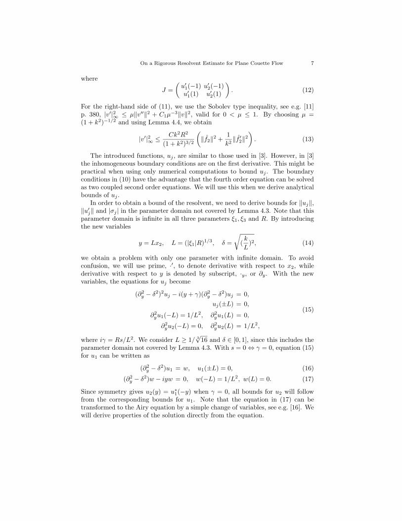
On a Rigorous Resolvent Estimate for Plane Couette Flow 7
where
J =
(
u′1(−1) u′
2(−1)u′
1(1) u′2(1)
)
. (12)
For the right-hand side of (11), we use the Sobolev type inequality, see e.g. [11]p. 380, |v′|2∞ ≤ µ‖v′′‖2 + C1µ
−3‖v‖2, valid for 0 < µ ≤ 1. By choosing µ =(1 + k2)−1/2 and using Lemma 4.4, we obtain
|v′|2∞ ≤ Ck2R2
(1 + k2)3/2
(
‖f2‖2 +1
k2‖f ′
2‖2
)
. (13)
The introduced functions, uj , are similar to those used in [3]. However, in [3]the inhomogeneous boundary conditions are on the first derivative. This might bepractical when using only numerical computations to bound uj . The boundaryconditions in (10) have the advantage that the fourth order equation can be solvedas two coupled second order equations. We will use this when we derive analyticalbounds of uj .
In order to obtain a bound of the resolvent, we need to derive bounds for ‖uj‖,‖u′
j‖ and |σj | in the parameter domain not covered by Lemma 4.3. Note that thisparameter domain is infinite in all three parameters ξ1, ξ3 and R. By introducingthe new variables
y = Lx2, L = (|ξ1|R)1/3, δ =
√
(k
L)2, (14)
we obtain a problem with only one parameter with infinite domain. To avoidconfusion, we will use prime, ·′, to denote derivative with respect to x2, whilederivative with respect to y is denoted by subscript, ·y, or ∂y. With the newvariables, the equations for uj become
(∂2y − δ2)2uj − i(y + γ)(∂2
y − δ2)uj = 0,
uj(±L) = 0,(15)
∂2yu1(−L) = 1/L2, ∂2
yu1(L) = 0,
∂2yu2(−L) = 0, ∂2
yu2(L) = 1/L2,
where iγ = Rs/L2. We consider L ≥ 1/ 3√
16 and δ ∈ [0, 1], since this includes theparameter domain not covered by Lemma 4.3. With s = 0 ⇔ γ = 0, equation (15)for u1 can be written as
(∂2y − δ2)u1 = w, u1(±L) = 0, (16)
(∂2y − δ2)w − iyw = 0, w(−L) = 1/L2, w(L) = 0. (17)
Since symmetry gives u2(y) = u∗1(−y) when γ = 0, all bounds for u2 will follow
from the corresponding bounds for u1. Note that the equation in (17) can betransformed to the Airy equation by a simple change of variables, see e.g. [16]. Wewill derive properties of the solution directly from the equation.

8 P.-O. Asen and G. Kreiss JMFM
4.3. New analytical bounds
In this section, we derive new analytical bounds which give a sharp bound of theresolvent in all but a compact subset of the parameter domain. The results aresummarized in the following lemma.
Lemma 4.5. There is a constant C, independent of ξ1, ξ3 and R, such that if
both (|ξ1|R)2/3 ≥ ξ21 + ξ2
3 and |ξ1|R ≥ 403 hold, then for s = 0
‖u′2‖2 + ‖u2‖2 ≤ Ck2R2
(1 + k2)3/2
(
‖f2‖2 +1
k2‖f ′
2‖2
)
.
As was the case for Lemma 4.3, Lemma 4.5 gives the sharp bound of theresolvent, (7), by using Lemma 4.2 and (6). Note that with the variables (14),Lemma 4.3 and Lemma 4.5 cover all but the compact set L ∈ [1/ 3
√16, 40], δ ∈ [0, 1].
We will prove Lemma 4.5 by proving that for the parameter values covered andwith J given by (12), the solutions of (10) with s = 0 satisfy
‖J−1‖2∞(‖uj‖2 + ‖u′
j‖2) ≤ C, j = 1, 2, (18)
where C is independent of ξ1, ξ3 and R and ‖J−1‖∞ is the max-norm of thematrix J−1. Indeed, if (18) holds, then Lemma 4.5 follows by using Lemma 4.4,(11) and (13).
In order to prove (18), we consider (17) and (16). We will derive analyticalbounds which, after transforming back to the original variables, give (18). Theanalytical bounds will be obtained by first finding an approximate solution, wapp,of (17), then solving (16) with wapp on the right-hand side, and finally boundingthe errors made by the approximations. This will only be possible when L ≥ 40.
An approximate solution of (17) can be obtained by writing the equation as(
wy
w
)
y
=
(
0 δ2 + iy1 0
) (
wy
w
)
. (19)
When |y| is large, the eigenvalues of this matrix are well separated and the systemcan be diagonalized. Let us for a moment consider y ∈ [−L,−l0] where L > l0 > 0.Introduce new variables
(
wy
w
)
=
(
λ −λ1 1
)(
z1
z2
)
, (20)
where λ =√
δ2 + iy. From (19) and (20), the system for z = (z1, z2)T becomes
zy =
(
λ 00 −λ
)
z + ε
(
−b bb −b
)
z, (21)
where
ε = λ−20 , b = i
(
λ0
2λ
)2
, λ0 =√
δ2 − il0. (22)
In order to diagonalize (21), we use a special case of Lemma 2.6 in [9].
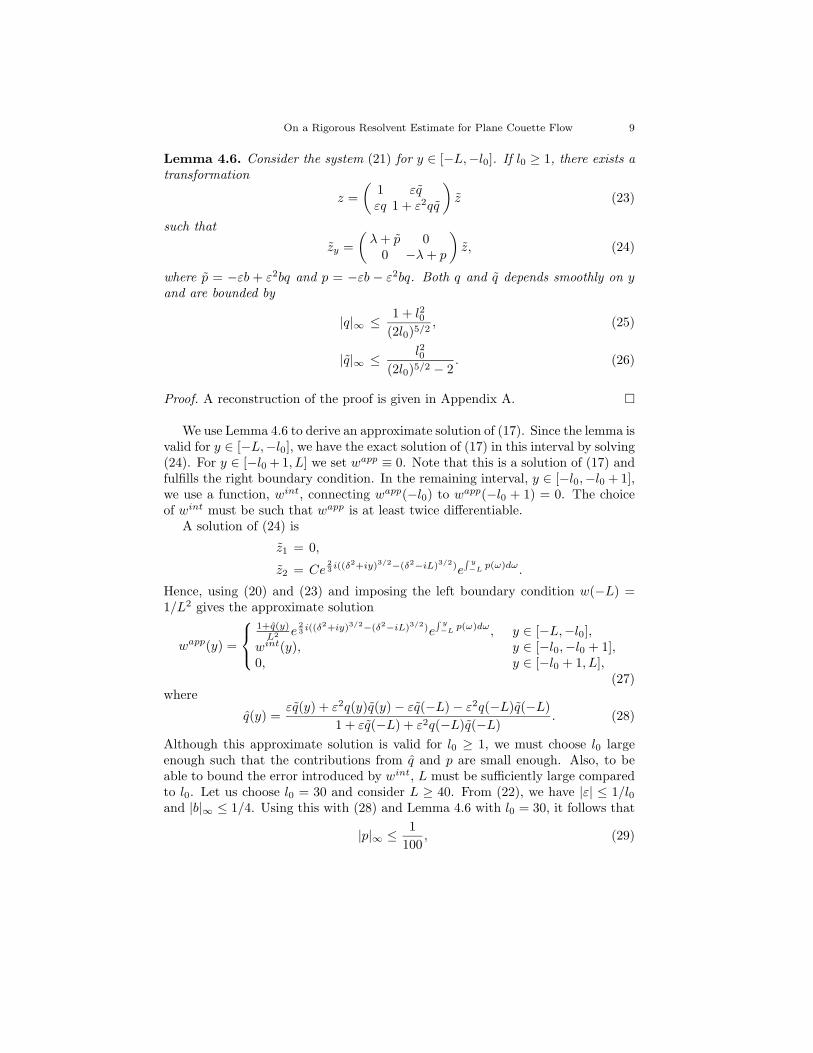
On a Rigorous Resolvent Estimate for Plane Couette Flow 9
Lemma 4.6. Consider the system (21) for y ∈ [−L,−l0]. If l0 ≥ 1, there exists a
transformation
z =
(
1 εqεq 1 + ε2qq
)
z (23)
such that
zy =
(
λ + p 00 −λ + p
)
z, (24)
where p = −εb + ε2bq and p = −εb − ε2bq. Both q and q depends smoothly on yand are bounded by
|q|∞ ≤ 1 + l20(2l0)5/2
, (25)
|q|∞ ≤ l20(2l0)5/2 − 2
. (26)
Proof. A reconstruction of the proof is given in Appendix A. ¤
We use Lemma 4.6 to derive an approximate solution of (17). Since the lemma isvalid for y ∈ [−L,−l0], we have the exact solution of (17) in this interval by solving(24). For y ∈ [−l0 + 1, L] we set wapp ≡ 0. Note that this is a solution of (17) andfulfills the right boundary condition. In the remaining interval, y ∈ [−l0,−l0 + 1],we use a function, wint, connecting wapp(−l0) to wapp(−l0 + 1) = 0. The choiceof wint must be such that wapp is at least twice differentiable.
A solution of (24) is
z1 = 0,
z2 = Ce2
3i((δ2+iy)3/2−(δ2−iL)3/2)e
∫ y−L
p(ω)dω.
Hence, using (20) and (23) and imposing the left boundary condition w(−L) =1/L2 gives the approximate solution
wapp(y) =
1+q(y)L2 e
2
3i((δ2+iy)3/2−(δ2−iL)3/2)e
∫ y−L
p(ω)dω, y ∈ [−L,−l0],wint(y), y ∈ [−l0,−l0 + 1],0, y ∈ [−l0 + 1, L],
(27)where
q(y) =εq(y) + ε2q(y)q(y) − εq(−L) − ε2q(−L)q(−L)
1 + εq(−L) + ε2q(−L)q(−L). (28)
Although this approximate solution is valid for l0 ≥ 1, we must choose l0 largeenough such that the contributions from q and p are small enough. Also, to beable to bound the error introduced by wint, L must be sufficiently large comparedto l0. Let us choose l0 = 30 and consider L ≥ 40. From (22), we have |ε| ≤ 1/l0and |b|∞ ≤ 1/4. Using this with (28) and Lemma 4.6 with l0 = 30, it follows that
|p|∞ ≤ 1
100, (29)

10 P.-O. Asen and G. Kreiss JMFM
|q|∞ ≤ 1
400. (30)
The rapid decay of wapp away from y = −L makes the choice of wint lessimportant. Therefore, the following derivation will be brief. The simplest choice isto take a fifth degree polynomial, thus ensuring continuity up to second derivative.We use three polynomials pn(y), n ∈ 0, 1, 2, satisfying ∂n
y pn(−l0) = 1 andotherwise homogeneous conditions up to second derivative at both ends. It iseasily verified that the polynomials are given by
p1(y) = 1 − 10(y + l0)3 + 15(y + l0)
4 − 6(y + l0)5,
p2(y) = (y + l0) − 6(y + l0)3 + 8(y + l0)
4 − 3(y + l0)5, (31)
p3(y) =1
2
(
(y + l0)2 − 3(y + l0)
3 + 3(y + l0)4 − (y + l0)
5)
.
Using these polynomials, wint can be written as
wint(y) =
2∑
n=0
∂ny wapp(−l0)pn(y), y ∈ [−l0,−l0 + 1]. (32)
From (27), we have
∂ywapp(−l0) =
(
qy(−l0)
1 + q(−l0)+ p(−l0) − λ0
)
wapp(−l0). (33)
Since l0 = 30 and δ ∈ [0, 1], we have δ2 ≤ l0/30 which gives |λ0| ≤√
l0(901/900)1/4.By differentiating (28) with respect to y and using Q = Q = 0 with Q and Q givenby (43) and (44), we obtain an expression for qy(−l0) in terms of q, q, ε, λ0, band p. Using Lemma 4.6 and (22), the parentheses on the right-hand side of (33)is easily bounded by 2
√l0 (it is actually bounded by 1.006
√l0, but the constant
is of minor importance due to the exponential decay of wapp(y)). Proceeding inthe same way, differentiating (27), replacing derivatives of q using (28), (43) and(44), differentiating p and λ and finally using the known bounds of all quantities,we obtain a bound of |∂2
ywapp(−l0)|. Summarizing, we have the following bounds
|∂ywapp(−l0)| ≤ 2√
l0|wapp(−l0)|,(34)
|∂2ywapp(−l0)| ≤ 2l0|wapp(−l0)|.
Now, using (30), (32) and (34) and integrating |pn(y)|, |pn(y)|2, |∂2ypn(y)|2, with
pn(y), n ∈ 0, 1, 2, given by (31), gives∫ −l0+1
−l0
|wint(y)|dy ≤ 3
L2|e 2
3i((δ2−il0)
3/2−(δ2−iL)3/2)e∫ −l0−L p(ω)dω|, (35)
∫ −l0+1
−l0
|wint(y)|2dy ≤ 7
L4|e 2
3i((δ2−il0)
3/2−(δ2−iL)3/2)e∫ −l0−L p(ω)dω|2, (36)
∫ −l0+1
−l0
|∂2ywint(y)|2dy ≤ 3000
L4|e 2
3i((δ2−il0)
3/2−(δ2−iL)3/2)e∫ −l0−L p(ω)dω|2. (37)

On a Rigorous Resolvent Estimate for Plane Couette Flow 11
In (36) we used the inequality |p0(y) + p1(y) + p2(y)|2 ≤ 4|p0(y)2| + 2|p1(y)|2 +4|p2(y)|2. This was also used for (37) with ∂2
ypn instead of pn.This completes the derivation of an approximate solution of (17). Since (16)
is a constant coefficient problem, there is a well known solution formula. Solving(16) using the approximate solution wapp gives the following lemma.
Lemma 4.7. If L ≥ 40, l0 = 30 and δ ∈ [0, 1], the solution of
(∂2y − δ2)uapp
1 = wapp, y ∈ [−L,L], (38)
with wapp given by (27) and the boundary conditions uapp1 (±L) = 0 satisfies
‖∂yuapp1 ‖2 + ‖uapp
1 ‖2 ≤ C
L5,
|∂yuapp1 (−L)| ≥ 0.6
L5/2,
|∂yuapp1 (L)| ≤ 1.4
L4,
where C is independent of L and δ, and ‖ · ‖ is the L2- norm over y ∈ [−L,L].
Proof. The proof is given in Appendix B. ¤
In order to bound the errors made by using the approximate solution, wapp, weintroduce a new function. Let u1 = uapp
1 + ucorr1 . From (16), (17) and (38), ucorr
1
must satisfy
(∂2y − δ2)2ucorr
1 − iy(∂2y − δ2)ucorr
1 = −((∂2y − δ2)wapp − iywapp) ≡ F (y),
(39)ucorr
1 (±L) = ∂2yucorr
1 (±L) = 0.
Integration by parts yields the following lemma.
Lemma 4.8. The solution ucorr1 of (39) satisfies
‖ucorr1 ‖2 ≤ 4096L8‖F‖2,
‖∂yucorr1 ‖2 ≤ 512L6‖F‖2,
‖∂2yucorr
1 ‖2 ≤ 64L4‖F‖2,
where ‖ · ‖ is the L2-norm over y ∈ [−L,L].
Proof. The proof is given in Appendix C. ¤
In order to estimate the contribution from ucorr1 , we need to bound ‖F‖. Re-
member that the construction of wapp was done such that wapp solves (17) wheny /∈ [−l0,−l0 + 1]. Hence, the only contribution to F is from wint and we obtainthe following lemma.

12 P.-O. Asen and G. Kreiss JMFM
Lemma 4.9. Consider wapp given by (27) and F (y) given by (39). If L ≥ 40,l0 = 30 and δ ∈ [0, 1], then F (y) satisfies
‖F‖2 ≤ 25000
L4e0.94(l
3/2
0−L3/2),
where ‖ · ‖ is the L2-norm over y ∈ [−L,L].
Proof. The proof is given in Appendix D. ¤
By Lemma 4.9, all bounds in Lemma 4.8 are exponentially small. Evaluatingnumerically with l0 = 30 and L ≥ 40 gives
L8‖∂2yucorr
1 ‖2 + L8‖∂yucorr1 ‖2 + L5‖ucorr
1 ‖2 ≤ 10−12,(40)
|∂yucorr1 (±L)| ≤ 10−5
L4,
where the last result follows from the Sobolev type inequality, see e.g. [11] pp. 378–379,
|∂yucorr1 |2∞ ≤ µ‖∂2
yucorr1 ‖2 +
(
1
µ+
1
2L
)
‖∂yucorr1 ‖2, µ > 0.
Using these results, we are finally able to prove Lemma 4.5.
Proof of Lemma 4.5. With the variables (14), the parameter domain covered byLemma 4.5 is covered by L ≥ 40 and δ ∈ [0, 1]. Since u1 = uapp
1 + ucorr1 , using
Lemma 4.7, (40) and transforming from y to x2 gives
(|ξ1|R)4/3‖u′1‖2 + (|ξ1|R)2‖u1‖2 ≤ C,
|u′1(−1)| ≥ 0.5
(|ξ1|R)1/2, (41)
|u′1(1)| ≤ 1.5
(|ξ1|R),
where ‖ · ‖ is the L2-norm over x2 ∈ [−1, 1]. Here we have used, from (14), that(|ξ1|R)1/3‖u1‖2
x2= ‖u1‖2
y and (|ξ1|R)−1/3‖u′1‖2
x2= ‖∂yu1‖2
y, where subscriptsdenotes the domain over which the L2-norm is evaluated. The last two bounds of(41) give, using (12) and the symmetry u2(x2) = u∗
1(−x2), the bound
‖J−1‖2∞ ≤
∣
∣
∣
∣
|u′1(−1)| + |u′
1(1)||u′
1(−1)|2 − |u′1(1)|2
∣
∣
∣
∣
2
≤ C(|ξ1|R). (42)
The bound (18) follows from (41) and (42). As previously mentioned, Lemma 4.5follows from (18) by using Lemma 4.2 and (6). ¤
This implies that Theorem 4.1 is proved in the parameter domain covered byLemma 4.3 and Lemma 4.5.

On a Rigorous Resolvent Estimate for Plane Couette Flow 13
4.4. Numerical computations
It remains to prove Theorem 4.1 in the parameter domain |ξ1|R ∈ [1/16, 403] and(|ξ1|R)2/3 ≥ ξ2
1 +ξ23 . Hence, we want to show that (18) holds also in this parameter
domain. Using the variables (14), it is enough to consider L ∈ [1/ 3√
16, 40] andδ ∈ [0, 1], which is a bounded parameter domain. Here we rely on numericalcomputations. We solve (16) and (17) using second order finite differences, andthen compute the quantities on the left-hand side of (18). Note that we only wishto bound the left-hand side of (18) by any constant. Since (16) and (17) are linearordinary differential equations with δ only appearing in front of lower order terms,we would not expect the solution or its derivatives to become infinite on a domainwith length bounded from below and from above. A potential problem of fulfilling(18) is that J might become singular. However, since the parameter domain issmall, the solution can easily be sufficiently resolved. We computed solutionsto (16) and (17) for the parameter values δ ∈ [0, 1] with step size dδ = 0.005,L ∈ [0.3, 10] with step size dL = 0.1, L ∈ [11, 15] with step size dL = 1, andL ∈ [20, 40] with step size dL = 5. After transforming from y to x2, we computedthe quantities on the left-hand side of (18) and the results are shown in Fig. 1. Thefigures do not contain all the parameter values considered. We used the spatialdiscretization h = 0.005 of y ∈ [−L,L] in all computations. Clearly, (18) is fulfilledalso for L ∈ [1/ 3
√16, 40] and δ ∈ [0, 1] and Theorem 4.1 is proved. We note that
in order for this part of the proof to be rigorous, validated methods using intervalarithmetic should be used in the numerical computations.
0
10
20
30
40 0
0.2
0.4
0.6
0.8
1
10−4
10−3
10−2
10−1
100
L
05
1015
2025
3035
40
0
0.2
0.4
0.6
0.8
1
100
101
102
103
L
Fig. 1. Numerical computations in the parameter domain L ∈ [1/ 3√
16, 40], δ ∈ [0, 1]. The leftfigure shows ‖u1‖ + ‖u′
1‖ and the right figure shows ‖J−1‖∞. Here ‖ · ‖ denotes the L2-norm
over x2 ∈ [−1, 1].
δ δ

14 P.-O. Asen and G. Kreiss JMFM
Remark. We found that already at L ≥ 3, ‖J−1‖∞ behaves like L3/2, as predictedby (42). Also, ‖u1‖ shows good agreement with the, from (41), asymptotic L−3
for L ≥ 10. However, the predicted behavior of L−2 for ‖u′1‖ is not sharp. Instead,
we found that ‖u′1‖ is proportional to L−9/4.
In order to ensure that the solutions were sufficiently resolved, we used severaldifferent discretizations of y ∈ [−L,L]. Let uh denote the solution on a meshwith step size h and rh denote the restriction to a mesh with step size h. Weestimated the error in the solutions by eh = uh − rhuh/2 and similarly for theerror in the derivative, ∂yeh. For J−1, the error, eJ
h , was estimated in the sameway, though without use of any restriction. Figure 2 shows the estimated errorsas function of the step size, h, for L = 40 and δ = 0. Similar plots were obtainedfor many different values of L and δ. Figure 2 indicates that the solution issufficiently resolved when h = 0.005 and, as expected, that the method is secondorder accurate.
10−3
10−2
10−1
100
10−12
10−10
10−8
10−6
10−4
10−2
100
102
104
h
Fig. 2. Estimated error as function of step size, h. The solid line is ‖eh‖h, the dashed line is‖∂yeh‖h and the dash-dotted line is ‖eJ
h‖∞. Here, ‖ · ‖h denotes the discrete L2-norm overy ∈ [−L, L].
A simple analysis shows that accurate solutions to (16) and (17) are difficultto obtain numerically when L is large. Consider the case δ = 0. Then, (16) isjust the Poisson equation, which is easily solved if w is sufficiently resolved. Forlarge L, we have by (27) that L2|∂yw(−L)| ∼ L1/2. Since L2w(−L) = 1, we needa spatial step size h ∼ L−1/2 to resolve w near the left boundary. Using a uniformmesh to discretize y ∈ [−L,L], the computational complexity, N , will be at least

On a Rigorous Resolvent Estimate for Plane Couette Flow 15
N ∼ L3/2. Although this can be reduced by using adaptive methods, the problemis increasingly ill-conditioned with growing L. However, in the parameter domainL ∈ [1/ 3
√16, 40], δ ∈ [0, 1], the solution is easily resolved using standard numerical
techniques.
5. Discussion
We have shown that the L2-norm of the resolvent for plane Couette flow is pro-portional to R2 at s = 0. This is known to be a sharp bound in three spacedimensions, see e.g. [10]. The two dimensional result R ∼ R, which is also sharp,follows from considering the case of no variation in the span wise direction, see theremark after Lemma 4.3. The proof is rigorous outside a compact subset of theparameter domain. This compact set can be reduced to a finite set of parametervalues, [2]. Using validated numerical methods in this finite set would result ina rigorous proof of the resolvent bound in the entire parameter domain. This issomething we hope to address in the near future.
In order to obtain a bound of the resolvent in the entire unstable half plane, itis enough to consider s with Re s = 0. This is due to the maximum principle andanalytical bounds in parts of the unstable half plane, see e.g. [8]. All results priorto Lemma 4.5 are valid for all s with Re s ≥ 0. For imaginary s, we can derive thebound (18) for uapp
j by using the transformation y = y + γ, γ = R Im s/L2. Theonly result that does not hold for Im s 6= 0 is (40), since the exponential term inLemma 4.9 will contain (L−γ)3/2, while we still will have high powers of L in thebounds in Lemma 4.8. Thus, we need to use a different strategy when boundingthe errors introduced by using the approximate solution.
Appendix A. Reconstruction of the Proof of Lemma 4.6
Introducing (23) into (21) gives
zy =
(
λ − εb + ε2bq + ε2qQ ε(ε2q2Q − Q)−εQ −λ − εb − ε2bq − ε2qQ
)
z,
where
Q = qy + 2λq + ε2bq2 − b, (43)
Q = qy − 2(λ + ε2bq)q − b. (44)
Solving Q = 0 and Q = 0 will give the desired result. Consider the linear equation
qly = a(y)ql + f(y), y ∈ [−L,−l0],
ql(−L) = 0,
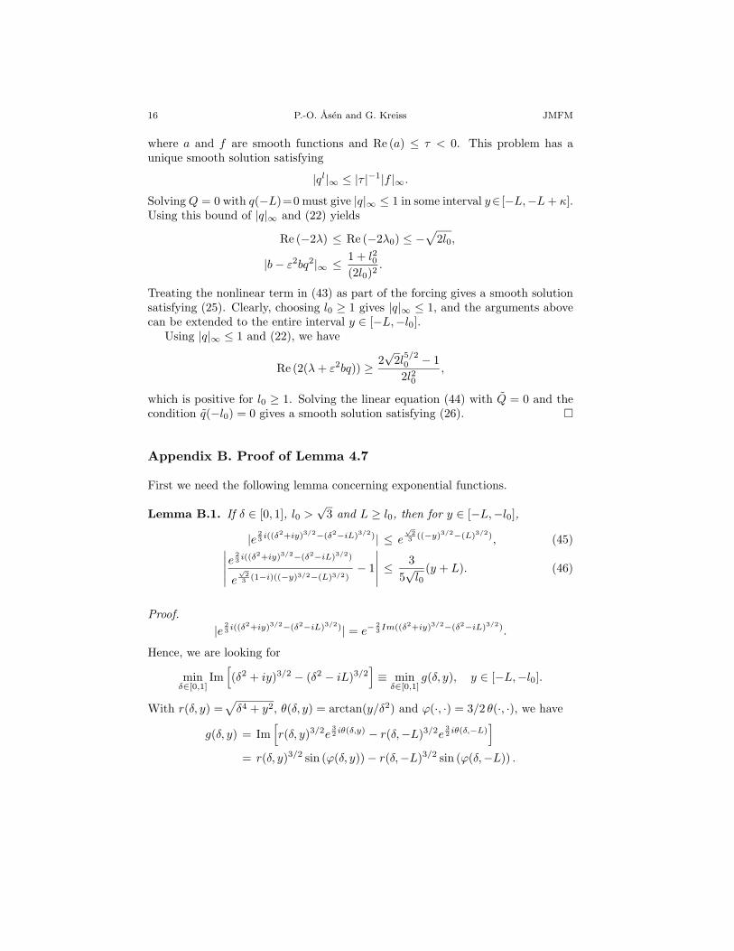
16 P.-O. Asen and G. Kreiss JMFM
where a and f are smooth functions and Re (a) ≤ τ < 0. This problem has aunique smooth solution satisfying
|ql|∞ ≤ |τ |−1|f |∞.
Solving Q = 0 with q(−L)=0 must give |q|∞ ≤ 1 in some interval y∈ [−L,−L + κ].Using this bound of |q|∞ and (22) yields
Re (−2λ) ≤ Re (−2λ0) ≤ −√
2l0,
|b − ε2bq2|∞ ≤ 1 + l20(2l0)2
.
Treating the nonlinear term in (43) as part of the forcing gives a smooth solutionsatisfying (25). Clearly, choosing l0 ≥ 1 gives |q|∞ ≤ 1, and the arguments abovecan be extended to the entire interval y ∈ [−L,−l0].
Using |q|∞ ≤ 1 and (22), we have
Re (2(λ + ε2bq)) ≥ 2√
2l5/20 − 1
2l20,
which is positive for l0 ≥ 1. Solving the linear equation (44) with Q = 0 and thecondition q(−l0) = 0 gives a smooth solution satisfying (26). ¤
Appendix B. Proof of Lemma 4.7
First we need the following lemma concerning exponential functions.
Lemma B.1. If δ ∈ [0, 1], l0 >√
3 and L ≥ l0, then for y ∈ [−L,−l0],
|e 2
3i((δ2+iy)3/2−(δ2−iL)3/2)| ≤ e
√2
3((−y)3/2−(L)3/2), (45)
∣
∣
∣
∣
∣
e2
3i((δ2+iy)3/2−(δ2−iL)3/2)
e√
2
3(1−i)((−y)3/2−(L)3/2)
− 1
∣
∣
∣
∣
∣
≤ 3
5√
l0(y + L). (46)
Proof.
|e 2
3i((δ2+iy)3/2−(δ2−iL)3/2)| = e−
2
3Im((δ2+iy)3/2−(δ2−iL)3/2).
Hence, we are looking for
minδ∈[0,1]
Im[
(δ2 + iy)3/2 − (δ2 − iL)3/2]
≡ minδ∈[0,1]
g(δ, y), y ∈ [−L,−l0].
With r(δ, y) =√
δ4 + y2, θ(δ, y) = arctan(y/δ2) and ϕ(·, ·) = 3/2 θ(·, ·), we have
g(δ, y) = Im[
r(δ, y)3/2e3
2iθ(δ,y) − r(δ,−L)3/2e
3
2iθ(δ,−L)
]
= r(δ, y)3/2 sin (ϕ(δ, y)) − r(δ,−L)3/2 sin (ϕ(δ,−L)) .

On a Rigorous Resolvent Estimate for Plane Couette Flow 17
Differentiating with respect to δ gives
∂g
∂δ= 3δ(h(δ, y) − h(δ,−L)),
h(δ, y) =− cos (ϕ(δ, y)) y + sin (ϕ(δ, y)) δ2
(δ4 + y2)1/4.
When l0 > tan(π/3) =√
3 and δ ∈ [0, 1], we have θ(δ, y) ∈ [−π/2,−π/3) ∀y ∈[−L,−l0], i.e. ϕ(δ, y) ∈ [−3π/4,−π/2). This gives h(δ, y) ≤ 0. Also, since
∂h
∂y= δ
3
2
δ4 cos(ϕ(δ, y)) + 2yδ2 sin(ϕ(δ, y)) − y2 cos(ϕ(δ, y))
(δ4 + y2)5/4,
which is positive for y < −√
3, we have that h(δ,−L) ≤ h(δ, y), giving ∂g/∂δ ≥ 0.Hence, g(δ, y) is minimized with respect to δ at δ = 0 ∀y ∈ [−L,−
√3), and (45)
follows.Taylor expansion of the exponent around δ = 0 gives
e2
3i((δ2+iy)3/2−(δ2−iL)3/2) = e
√2
3(1−i)((−y)3/2−L3/2)R(δ, y). (47)
From (45), it follows that |R(δ, y)| ≤ 1. Also, since R(δ,−L) − 1 = 0, we have|R(δ, y) − 1| ≤ |∂R/∂y|∞(y + L). Differentiating (47) with respect to y yields
∂R
∂y=
(
−√
δ2 + iy − 1√2(−1 + i)
√−y
)
R(δ, y).
Taylor expansion gives
√
δ2 + iy|δ=0 =1√2(1 − i)
√−y +i
2√
2(1 − i)
1√−yδ2 − 5δ4
128(ξ(y)2 + iy)7/2,
where ξ(y) ∈ [0, δ]. Using this, we obtain∣
∣
∣
∣
∂R
∂y
∣
∣
∣
∣
≤ 1
2√−y
+5
128√−y
∣
∣
∣
∣
δ4√−y
(ξ(y)2 + iy)7/2
∣
∣
∣
∣
<3
5√−y
,
i.e. |∂R/∂y|∞ < 3/(5√
l0) and (46) follows. ¤
We also need some general results concerning integrals.
Lemma B.2. If l0 = 30, L ≥ 40, y ∈ [−L,−l0], |β| ≥√
2/23 and arg β = −π/4or arg β = 0, then
I(y, β) ≡∫ −l0
y
eβ((−σ)3/2−L3/2)dσ = f(−y, β) − f(l0, β),
f(−y, β) =2eβ((−y)3/2−L3/2)
3β√−y
(
1 +1
3β(−y)3/2+ ε2(−β(−y)3/2)
)
,
where ε2(z) is bounded by
|ε2(z)| ≤ 1
|z|2 . (48)
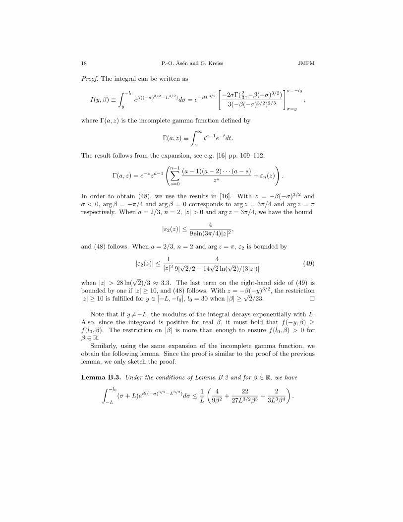
18 P.-O. Asen and G. Kreiss JMFM
Proof. The integral can be written as
I(y, β) ≡∫ −l0
y
eβ((−σ)3/2−L3/2)dσ = e−βL3/2 −2σΓ( 23 ,−β(−σ)3/2)
3(−β(−σ)3/2)2/3
]σ=−l0
σ=y
,
where Γ(a, z) is the incomplete gamma function defined by
Γ(a, z) ≡∫ ∞
z
ta−1e−tdt.
The result follows from the expansion, see e.g. [16] pp. 109–112,
Γ(a, z) = e−zza−1
(
n−1∑
s=0
(a − 1)(a − 2) · · · (a − s)
zs+ εn(z) .
In order to obtain (48), we use the results in [16]. With z = −β(−σ)3/2 andσ < 0, arg β = −π/4 and arg β = 0 corresponds to arg z = 3π/4 and arg z = πrespectively. When a = 2/3, n = 2, |z| > 0 and arg z = 3π/4, we have the bound
|ε2(z)| ≤ 4
9 sin(3π/4)|z|2 ,
and (48) follows. When a = 2/3, n = 2 and arg z = π, ε2 is bounded by
|ε2(z)| ≤ 1
|z|24
9[√
2/2 − 14√
2 ln(√
2)/(3|z|)](49)
when |z| > 28 ln(√
2)/3 ≈ 3.3. The last term on the right-hand side of (49) isbounded by one if |z| ≥ 10, and (48) follows. With z = −β(−y)3/2, the restriction|z| ≥ 10 is fulfilled for y ∈ [−L,−l0], l0 = 30 when |β| ≥
√2/23. ¤
Note that if y 6=−L, the modulus of the integral decays exponentially with L.Also, since the integrand is positive for real β, it must hold that f(−y, β) ≥f(l0, β). The restriction on |β| is more than enough to ensure f(l0, β) > 0 forβ ∈ R.
Similarly, using the same expansion of the incomplete gamma function, weobtain the following lemma. Since the proof is similar to the proof of the previouslemma, we only sketch the proof.
Lemma B.3. Under the conditions of Lemma B.2 and for β ∈ R, we have
∫ −l0
−L
(σ + L)eβ((−σ)3/2−L3/2)dσ ≤ 1
L
(
4
9β2+
22
27L3/2β3+
2
3L3β4
)
.
On a Rigorous Resolvent Estimate for Plane Couette Flow 19
Proof. The integral can be written as
∫ −l0
−L
(σ + L)eβ((−σ)3/2−L3/2)dσ = e−βL3/2 2√−σeβ(−σ)3/2
3β
+2√−σΓ( 1
3 − β(−σ)3/2)
9β(−β(−σ)3/2)1/3− 2σLΓ( 2
3 ,−β(−σ)3/2)
3(−β(−σ)3/2)2/3
]σ=−l0
σ=−L
.
Now, the same expansion of the incomplete gamma function is used as in the previ-ous lemma. The first term in the brackets above indicates that the integral shouldbe proportional to
√L/β. However, this term will be canceled when expanding
Γ( 23 ,−β(−σ)3/2). Noting that the terms containing l0 can be omitted due to their
sign, the result follows. ¤
Finally, we need the following result for products of exponential functions.
Lemma B.4. Given γ > 0, β > 0, l0 > 0 and CL ≥ l0, if β∗ satisfies
β∗ ≤ β − γ(CL − l0)
C3/2L − l
3/20
,
then for all L ≥ CL
eγ(y+L)+β((−y)3/2−L3/2) ≤ eβ∗((−y)3/2−L3/2), ∀y ∈ [−L,−l0]. (50)
Note that if CL is sufficiently large, β∗ can be chosen to be positive.
Proof. Obviously, it is enough to consider y∈(−L,−l0]. Then (50) is equivalent to
β∗ ≤ γ(y + L)
(−y)3/2 − L3/2+ β, ∀y ∈ (−L,−l0].
Note that the first term on the right-hand side is always negative. Differentiatingwith respect to y gives
∂
∂y
(
γ(y + L)
(−y)3/2 − L3/2
)
= −γ2L3/2 + (−y)3/2 − 3
√−yL
2((−y)3/2 − L3/2)2≡ −γ
f
g.
Since f(−L) = 0 and ∂f/∂y = 3(y + L)/(2√−y) > 0 for y ∈ (−L,−l0], we have
f, g > 0, i.e. the hardest constraint on β∗ is at y = −l0. Clearly, if β∗ is chosenfor L = L∗, the inequality also holds ∀L ≥ L∗ and the result follows. ¤
Now we have the lemmas needed for bounding the various norms. When weuse β and γ, they denote constants in an exponential term on the same form asthe left-hand side of (50). Note that β must not always be real, e.g. when usingLemma B.2. If not stated, we assume that l0 = 30, L ≥ 40 and δ ∈ [0, 1].

20 P.-O. Asen and G. Kreiss JMFM
The solution of (38) can be written as
uapp1 (y) = uh(y) + up1
(y) + up2(y),
where
uh(y) =sinh(δ(y − L))
sinh (2δL)
∫ −l0+1
−L
1
δsinh(δ(σ + L))wapp(σ)dσ,
up1(y) = −1
δsinh(δ(y + L))
∫ −l0+1
y
cosh(δ(σ + L))wapp(σ)dσ, (51)
up2(y) =
1
δcosh(δ(y + L))
∫ −l0+1
y
sinh(δ(σ + L))wapp(σ)dσ.
We start with proving the bounds of |∂yuapp1 (±L)|. From this, most of the results
for the norms will follow. The derivative at y = −L can be written as
∂yuapp1 (−L) =
∫ −l0+1
−L
sinh(δ(σ − L))
sinh(2δL)wapp(σ)dσ. (52)
When σ ∈ [−L,−l0], we rewrite wapp given by (27) as
wapp = wapp + wapp(we − 1), (53)
where
wapp(σ) =1 + q(σ)
L2e
2
3i((δ2+iσ)3/2−(δ2−iL3/2)),
we(σ) = e∫ σ−L
p(ω)dω.
Using (45) we have
|wapp(σ)| ≤ 1 + Cq
L2e
√2
3((−σ)3/2−L3/2),
where, from (30), Cq = 1/400. From (52) and (53) we obtain
|∂yuapp1 (−L)| ≥
∣
∣
∣
∣
∣
∫ −l0
−L
wapp(σ)dσ
∣
∣
∣
∣
∣
−∫ −l0
−L
(
sinh(δ(σ − L))
sinh(2δL)+ 1
)
|wapp(σ)|dσ
(54)
−∫ −l0
−L
|wapp(σ)||we(σ) − 1|dσ −∫ −l0+1
−l0
|wint(σ)|dσ ≡ I1 − I2 − I3 − Iint,
where we have used | sinh(δ(σ − L))/ sinh(2δL)| ≤ 1 in I3 and Iint. Consider firstI2. Let
v(δ, σ) =
(
sinh(δ(σ − L))
sinh(2δL)+ 1
)
.
Then v(δ,−L) = 0 and∣
∣
∣
∣
∂v
∂σ
∣
∣
∣
∣
=
∣
∣
∣
∣
δ cosh(δ(σ − L))
sinh(2δL)
∣
∣
∣
∣
≤∣
∣
∣
∣
δ cosh(2δL)
sinh(2δL)
∣
∣
∣
∣
.

On a Rigorous Resolvent Estimate for Plane Couette Flow 21
By considering the cases δL ≤ 1 and δL > 1, it is easily shown that |∂σv| ≤ 1.05,i.e.
|v(δ, σ)| < 1.05(σ + L).
With L ≥ 40 and β =√
2/3, the parentheses on the right-hand side of the inequal-ity in Lemma B.3 is bounded by 2.04, giving
I2 ≤ 1.05(1 + Cq)2.04
L3≤ 2.15
L3. (55)
In order to bound I3, we wish to bound |we−1| using, from (29), |p|∞ ≤ 1/100.Note that we(−L)− 1 = 0. Obviously, given two smooth, real functions f, g, suchthat f(−L) = g(−L) = 0 and |∂σf(σ)| ≤ ∂σg(σ) > 0 for σ ∈ [−L,−l0], it followsthat |f(σ)| ≤ g(σ) on the same interval. Also, for a complex function we have| ∂σ|f(σ)| | ≤ |∂σf(σ)|, which can be shown using polar coordinates. Thus, wehave
|∂σ|e∫ σ−L
p(ω)dω − 1|| ≤ |∂σ(e∫ σ−L
p(ω)dω − 1)| = |p(σ)e∫ σ−L
p(ω)dω|≤ |p|∞e|p|∞(σ+L) ≤ 2|p|∞ cosh(|p|∞(σ + L)).
Using |p|∞ ≤ 1/100 < 1, i.e. cosh(|p|∞(σ + L)) ≤ cosh(σ + L), it follows that
|we(σ) − 1| ≤ 2|p|∞ sinh(σ + L). (56)
For σ ∈ [−L,−L + α], we have sinh(σ + L) ≤ sinh(α)(σ + L)/α. Using this andLemma B.3 with β =
√2/3 gives
∣
∣
∣
∣
∣
∫ −L+α
−L
sinh(σ + L)|wapp(σ)|dσ
∣
∣
∣
∣
∣
≤ (1 + Cq)C1
L3,
(57)
C1 =sinh(α)
α
(
2 +11√2L3/2
+27
2L3
)
.
For the rest of the interval, we have sinh(σ+L) ≤ eσ+L/2. When using Lemma B.4with β =
√2/3, γ = 1, l0 = 30 and L ≥ 40, it is sufficient to choose β∗ =
√2/4.
Using this with Lemma B.2 gives∣
∣
∣
∣
∣
∫ −l0
−L+α
sinh(σ + L)|wapp(σ)|dσ
∣
∣
∣
∣
∣
≤ 1 + Cq
2L2|f(L − α,
√2/4) − f(l0,
√2/4)|.
(58)Since f(l0,
√2/4) > 0, this term can be ignored. Thus, from (57) and (58) we have
∣
∣
∣
∣
∣
∫ −l0
−L
sinh(σ + L)|wapp(σ)|dσ
∣
∣
∣
∣
∣
≤ 1 + Cq
L3
(
C1 +L
2f(L − α,
√2/4)
)
,
f(L − α,√
2/4) ≤ 4√
2e√
2
4((L−α)3/2−L3/2)
3√
(L − α)
(
1 +2√
2
3(L − α)3/2+
8
(L − α)3
)
,
where C1 is given by (57). It is clear that C1 is decreasing with growing L andincreasing with growing α. Also, for sufficiently large L and α, Lf(L − α,
√2/4)

22 P.-O. Asen and G. Kreiss JMFM
is decreasing with both growing α and growing L, since the decreasing exponen-tial term will eventually dominate. Simple numerical experiments show that forα ≥ 0.5, Lf(L − α,
√2/4) is decreasing with L for L ≥ 40. Taking α = 1 and
evaluating the constants numerically at L = 40 gives∣
∣
∣
∣
∣
∫ −l0
−L
sinh(σ + L)|wapp(σ)|dσ
∣
∣
∣
∣
∣
≤ 2.611 + Cq
L3≤ 2.62
L3. (59)
Using this and (56) with the definition (54) of I3 gives
I3 ≤ 2|p|∞2.62
L3≤ 0.053
L3. (60)
Note that if β ≥ 0.18, an estimate similar to (59) can be derived, although witha different constant on the right-hand side. Indeed, β ≥ 0.18 is enough to ensureβ∗ ≥
√2/23 when using Lemma B.4 with γ = 1. Hence, Lemma B.2 may be used,
and we obtain a bound similar to (58). Choosing α > 0, the right-hand side of (58)is exponentially small, although possibly with a large constant. Also, β ≥ 0.18 isenough to derive an estimate similar to (57), again possibly with a large constanton the right-hand side. Hence, (59) is valid for all β ≥ 0.18 with a different valueof the constant. We will use this later when bounding the norms.
In order to bound I1 from below, we rewrite I1 as
I1 ≥∣
∣
∣
∣
∣
∫ −l0
−L
wapp(σ)dσ
∣
∣
∣
∣
∣
−∫ −l0
−L
|wapp(σ)|∣
∣
∣
∣
wapp(σ)
wapp(σ)− 1
∣
∣
∣
∣
dσ ≡ II1 − III
1 ,
where
wapp(σ) =1 + q(σ)
L2e
√2
3(1−i)((−σ)3/2−L3/2).
From (46) and Lemma B.3 with β =√
2/3, L ≥ 40 and l0 = 30, we have
III1 ≤ 3
5√
l0
∫ −l0
−L
(σ + L)|wapp(σ)|dσ ≤ 2.04(1 + Cq)3
5√
l0L3≤ 0.23
L3. (61)
For II1 , we have
II1 ≥ 1
L2
∣
∣
∣
∣
∣
∫ −l0
−L
e√
2
3(1−i)((−σ)3/2−L3/2)dσ
∣
∣
∣
∣
∣
− Cq
L2
∫ −l0
−L
e√
2
3((−σ)3/2−L3/2)dσ.
Using Lemma B.2 with β = (1 − i)√
2/3 and β =√
2/3, we obtain
II1 ≥ 1
L5/2
(
∣
∣
∣
∣
1 +1 + i
2√
2L3/2
∣
∣
∣
∣
−∣
∣
∣
∣
3
2L3
∣
∣
∣
∣
−√
L√l0
e√
2
3(l
3/2
0−L3/2)
×∣
∣
∣
∣
∣
1 +1 + i
2√
2l3/20
+3
2l30
∣
∣
∣
∣
∣
− Cq
√2
∣
∣
∣
∣
1 +1√
2L3/2+
9
2L3
∣
∣
∣
∣
)
.

On a Rigorous Resolvent Estimate for Plane Couette Flow 23
Evaluating the parentheses for L ≥ 40, l0 = 30 and Cq = 1/400 gives
II1 ≥ 0.99
L5/2. (62)
For Iint, using (35) with (45) and then Lemma B.4 with β =√
2/3 and γ = |p|∞ =1/100, making it sufficient to choose β∗ = 0.47, gives
Iint ≤3
L2e0.47(l
3/2
0−L3/2) ≤ 1
L13, (63)
where the last inequality follows from numerical evaluation with l0 = 30 andL ≥ 40. From (54), (55), (60), (61), (62) and (63), we thus have
|∂yuapp1 (−L)| ≥ 1
L5/2(0.99 − 0.23 + 2.15 + 0.053√
L− 1
L21/2) ≥ 0.6
L5/2,
which proves the third bound of Lemma 4.7.At the right boundary, using δ/ sinh(2δL) ≤ 1/(2L), (59), (56) and the expres-
sion (53) for wapp, we obtain
|∂yuapp1 (L)| =
∣
∣
∣
∣
∣
δ
sinh(2δL)
∫ −l0+1
−L
1
δsinh(δ(σ + L))wapp(σ)dσ
∣
∣
∣
∣
∣
(64)
≤ 1
2L
(
2.62
L3+ 2|p|∞
∫ −l0
−L
sinh2(σ + L)|wapp(σ)|dσ +eL−l0+1
2Iint
)
,
where Iint is bounded by (63). Using Lemma B.4 with β = 0.47 and γ = 1 givesβ∗ = 0.35, which bounds the last term on the right-hand side of (64) by
eL−l0+1
2Iint ≤
3e
2L2e0.35(l
3/2
0−L3/2) ≤ 1
L10, (65)
where the last inequality is obtained by numerical evaluation. For the second termon the right-hand side of (64), proceeding as when deriving (59) gives
∫ −l0
−L
sinh2(σ + L)|wapp(σ)|dσ ≤ 1 + Cq
L3(sinh(α)C1 + |f(L − α,
√2/6)|)
(66)
≤ 5.79
L3,
where C1 is given by (57) and f(·, ·) is defined by Lemma B.2. The last inequalityin (66) follows from choosing α = 1.1, which is obtained by numerical experiments.Using (64), (65) and (66) yields
|∂yuapp1 (L)| ≤ 1
2L4
(
2.62 +5.79
50+
1
L7
)
≤ 1.4
L4,
which proves the fourth bound of Lemma 4.7.Since we are not interested in values of constants when bounding the norms,
we will give these proves in less detail. The constant C will be used to denote

24 P.-O. Asen and G. Kreiss JMFM
any constant independent of L and δ. The contribution from integrating overy ∈ [−l0,−l0 + 1], i.e. integrating over wint, will always be exponentially small.Therefore, we will only consider the contribution from wapp when y ∈ [−L,−l0].Also, instead of dividing wapp into wapp and we, we will use wapp directly.
Using (45) and Lemma B.4 with β =√
2/3 and γ = |p|∞ = 1/100, making itsufficient to chose β∗ = 0.47, we have
|wapp(y)| ≤ 1 + Cq
L2e0.47((−y)3/2−L3/2).
From (51) and assuming wint ≡ 0, we obtain
‖uh‖2 ≤∫ L
−L
∣
∣
∣
∣
sinh(δ(y − L))
sinh (2δL)
∣
∣
∣
∣
2∣
∣
∣
∣
∣
∫ −l0
−L
1
δsinh(δ(σ + L))|wapp(σ)|dσ
∣
∣
∣
∣
∣
2
dy.
As previously mentioned, (59) is valid also for β = 0.47, although with a slightlylarger constant. Also, we have
∣
∣
∣
∣
sinh(δ(y − L))
sinh (2δL)
∣
∣
∣
∣
2
≤∣
∣
∣
∣
y − L
2L
∣
∣
∣
∣
2
,
since for a fixed y ∈ (−L,L), the denominator grows faster than the numeratorwith δ. Using this and (59) gives
‖uh‖2 ≤ C
L6
∫ L
−L
∣
∣
∣
∣
y − L
2L
∣
∣
∣
∣
2
dy ≤ C
L5. (67)
Since up1= 0 for y ∈ [−l0, L] if we assume wint ≡ 0, we have
‖up1‖2 ≤
∫ −l0
−L
∣
∣
∣
∣
1
δsinh(δ(y + L))
∣
∣
∣
∣
2∣
∣
∣
∣
∣
∫ −l0
y
cosh(δ(σ + L))|wapp(σ)|dσ
∣
∣
∣
∣
∣
2
dy.
Using Lemma B.4 with β = 0.47 and γ = 1 gives β∗ =√
2/4. It follows fromLemma B.2 that
∣
∣
∣
∣
∣
∫ −l0
y
cosh(δ(σ + L))|wapp(σ)|dσ
∣
∣
∣
∣
∣
2
≤ C
L4e
√2
2((−y)3/2−L3/2). (68)
Since the exponential term decays faster than |wapp|, we may use the result from(66) which gives
‖up1‖2 ≤ C
L5. (69)
For up2we have
‖up2‖ ≤
∫ −l0
−L
| cosh(δ(y + L))|2∣
∣
∣
∣
∣
∫ −l0
y
1
δsinh(δ(σ + L))|wapp(σ)|dσ
∣
∣
∣
∣
∣
2
dy.

On a Rigorous Resolvent Estimate for Plane Couette Flow 25
Again, we consider two intervals. For the first interval, we have from (59)
∫ −L+α
−L
| cosh(δ(y + L))|2∣
∣
∣
∣
∣
∫ −l0
−L
1
δsinh(δ(σ + L))|wapp(σ)|dσ
∣
∣
∣
∣
∣
2
dy ≤ C
L6,
where C only depends on the choice of α. Using (68), since sinh(δ(σ + L))/δ <cosh(δ(σ + L)), bounding | cosh(δ(σ + L))|2 with an exponential function andusing Lemma B.2, the contribution from integrating over y ∈ [−L + α,−l0] isexponentially small. Hence, we have
‖up2‖2 ≤ C
L6. (70)
Using (67), (69) and (70) gives
‖u1‖2 ≤ C
L5,
which proves the first bound of Lemma 4.7.It remains to prove the bound of ‖∂yu1‖. Using (51), we can write the derivative
as∂yuapp
1 (y) = ∂yuh(y) + ∂yup1(y) + ∂yup2
(y),
where
∂yuh(y) = δcosh(δ(y − L))
sinh (2δL)
∫ −l0+1
−L
1
δsinh(δ(σ + L))wapp(σ)dσ,
∂yup1(y) = − cosh(δ(y + L))
∫ −l0+1
y
cosh(δ(σ + L))wapp(σ)dσ, (71)
∂yup2(y) = sinh(δ(y + L))
∫ −l0+1
y
sinh(δ(σ + L))wapp(σ)dσ.
As when bounding ‖u1‖, we only consider the contribution from wapp when y ∈[−L,−l0], since all contributions from integrating over y ∈ [−l0,−l0 + 1] is expo-nentially small. From (71) we have
‖∂yuh‖2 ≤∫ L
−L
∣
∣
∣
∣
δcosh(δ(y − L))
sinh (2δL)
∣
∣
∣
∣
2∣
∣
∣
∣
∣
∫ −l0
−L
1
δsinh(δ(σ + L))|wapp(σ)|dσ
∣
∣
∣
∣
∣
2
dy.
As was motivated previously, (59) also holds for wapp with a different constant.Hence, the integral over σ is bounded by C/L3. The integral over y can easily bebounded by one, giving
‖∂yuh‖2 ≤ C
L6. (72)
For ∂yup1, we have by (71)
‖∂yup1‖2 ≤
∫ −l0
−L
|cosh(δ(y + L))|2∣
∣
∣
∣
∣
∫ −l0
y
cosh(δ(σ + L))|wapp(σ)|dσ
∣
∣
∣
∣
∣
2
dy.

26 P.-O. Asen and G. Kreiss JMFM
When using Lemma B.4 with β = 0.47 and γ = 1, it is enough to choose β∗ = 0.35.Using this in the last integral above and using Lemma B.2, we obtain
∣
∣
∣
∣
∣
∫ −l0
−L
cosh(δ(σ + L))|wapp(σ)|dσ
∣
∣
∣
∣
∣
2
≤∣
∣
∣
∣
C
L2√
L
∣
∣
∣
∣
2
.
We use this when y ∈ [−L,−L+α]. From (68), Lemma B.4 and Lemma B.2, it fol-lows that the contribution from integrating over y ∈ [−L+α,−l0] is exponentiallysmall. Hence, we have
‖∂yup1‖2 ≤ C
L5. (73)
Finally, (71) gives
‖∂yup2‖2 ≤
∫ −l0
−L
|sinh(δ(y + L))|2∣
∣
∣
∣
∣
∫ −l0
y
sinh(δ(σ + L))|wapp(σ)|dσ
∣
∣
∣
∣
∣
2
dy.
Since sinh(δ(y + L)) < cosh(δ(y + L)), (73) also hold for ∂up2. Hence, using (72)
and (73), we have
‖∂yu1‖2 ≤ C
L5,
which proves the second bound of Lemma 4.7. ¤
Appendix C. Proof of Lemma 4.8
The proof is based on integration by parts, the Poincare inequality
‖h‖2 ≤ 4L2‖h′‖2,
valid for continuous differentiable functions h(x) defined on x ∈ [−L,L], such thath(±L) = 0, and the relation
ab ≤ 1
2µa2 +
µ
2b2, µ > 0, (74)
where a, b, µ ∈ R.We introduce the notation (∂2
y − δ2) ≡ ∆. Taking the inner product of (39)
with ∆ucorr1 , using integration by parts and taking absolute value of the real part
yields‖∂y∆ucorr
1 ‖2 + δ2‖∆ucorr1 ‖2 ≤ ‖∆ucorr
1 ‖‖F‖.Using (74) and the Poincare inequality for ∆ucorr
1 , we obtain
1
2‖∂y∆ucorr
1 ‖2 +
(
1
16L2+ δ2
)
‖∆ucorr1 ‖2 ≤ 4L2‖F‖2. (75)
Using integration by parts we have
‖∂yucorr1 ‖2 + δ2‖ucorr
1 ‖2 = |(ucorr1 , ∆ucorr
1 )| ≤ ‖ucorr1 ‖‖∆ucorr
1 ‖.
On a Rigorous Resolvent Estimate for Plane Couette Flow 27
Again, using (74) and the Poincare inequality for ucorr1 , we obtain the inequality
(75) with ‖∂yuapp1 ‖2 and ‖uapp
1 ‖2 on the left-hand side and ‖∆ucorr1 ‖2 on the right-
hand side. Combining the two inequalities gives the first two bounds of the lemma.The last bound follows from (75) and the relation
‖∆ucorr1 ‖2 = ‖∂2
yucorr1 ‖2 + 2δ2‖∂yucorr
1 ‖2 + δ4‖ucorr1 ‖2. ¤
Appendix D. Proof of Lemma 4.9
Since F (y) = 0 when y /∈ [−l0,−l0 + 1], we only need to consider the contributionfrom wint. The triangle inequality and the relation (a + b)2 ≤ 2a2 + 2b2 yield
‖F‖2 ≤ 4
∫ −l0+1
−l0
|∂2ywint(y)|2dy + (4δ4 + 2l20)
∫ −l0+1
−l0
|wint(y)|2dy.
Using (36), (37), δ ≤ 1 and l0 = 30, we have
‖F‖2 ≤ 25000
L4
∣
∣
∣e
2
3i((δ2−il0)
3/2−(δ2−iL)3/2)+|p|∞(y+L)∣
∣
∣
2
.
The lemma follow from using (45) and Lemma B.4 with γ = 2|p|∞ = 1/50,β = 2
√2/3, l0 = 30 and L ≥ 40, making it sufficient to choose β∗ = 0.94. ¤
References
[1] P.-O. Asen and G. Kreiss, A rigorous resolvent estimate for plane Couette flow, TechnicalReport TRITA-NA-0330, KTH, Stockholm, 2003.
[2] P.-O. Asen, A proof of a resolvent estimate for plane Couette flow by new analytical
and numerical techniques, Licentiate thesis, TRITA-NA-0427, KTH, Stockholm, 2004,http://www.nada.kth.se/∼aasen/Lic.pdf.
[3] P. Braz e Silva, Resolvent estimates for 2-dimensional perturbations of plane Couetteflow, Elec. J. Diff. Eq. 2002 (2002), 1–15.
[4] P. Braz e Silva, Resolvent estimates for plane Couette flow, SIAM J. Appl. Math. 65(2005), 667–683.
[5] S. J. Chapman, Subcritical transition in channel flows, J. Fluid Mech. 451 (2002), 35–97.[6] J. Denzler, A study of the spectral theory of the Orr–Sommerfeld equation for plane
Couette flow, Habilitationsschrift, TU Munchen, 1999.[7] P. G. Drazin and W. H. Reid, Hydrodynamic Stability, Cambridge University Press,
London, 1981.[8] N. Dunford and J. Schwartz, Linear operators, part I, Interscience Publ., New York,
1958.[9] G. Kreiss, H.-O. Kreiss and N. A. Petersson, On the convergence to steady state of
solutions of nonlinear hyperbolic-parabolic systems, SIAM J. Numer. Anal. 31 (1994),1577–1604.
[10] G. Kreiss, A. Lundbladh and D. S. Henningson, Bounds for threshold amplitudes insubcritical shear flows, J. Fluid Mech. 270 (1994), 175–198.
[11] H.-O. Kreiss and J. Lorenz, Initial-Boundary Value Problems and the Navier–Stokes
Equations, Pure Appl. Math. 136, Academic Press, Boston, 1989.[12] M. Liefvendahl, Stability results for viscous shock waves and plane Couette flow, PhD
thesis, KTH, Stockholm, 2001.

28 P.-O. Asen and G. Kreiss JMFM
[13] M. Liefvendahl and G. Kreiss, Analytical and numerical investigation of the resolventfor plane Couette flow, SIAM J. Appl. Math. 63 (2003), 801–817.
[14] M. Liefvendahl and G. Kreiss, Bounds for the threshold amplitude for plane Couetteflow, J. Nonlinear Math. Phys. 9 (2002), 311–324.
[15] A. Lundbladh, D. S. Henningson and S. C. Reddy, Threshold amplitudes for transitionin channel flows, in: M. Y. Hussaini, T. B. Gatski, and T. L. Jackson (eds.), Transition,
Turbulence, and Combustion, Vol. I, 309–318, Kluwer, Dordrecht, Holland, 1994.[16] F. W. J. Olver, Asymptotics and Special Functions, Academic Press, New York, 1974.[17] W. M. Orr, The stability or instability of the steady motions of a perfect liquid and of a
viscous liquid, Proc. of the Royal Irish Academy A27 (1907–1909), 9–138.[18] V. A. Romanov, Stability of plane-parallel Couette flow, Funct. Anal. Appl. 7 (1973),
137–146.[19] P. J. Schmid and D. S. Henningson, Stability and Transition in Shear Flows, Appl. Math.
Sci. 142, Springer, New York, 2001.[20] L. N. Trefethen, A. E. Trefethen, S. C. Reddy and T. A. Driscoll, Hydrodynamic
stability without eigenvalues, Science 261 (1993), 578–584.[21] V. I. Yudovich, The Linearization Method in Hydrodynamical Stability Theory, Trans.
Math. Monogr. 74, American Mathematical Society, Providence, RI, 1989.
Per-Olov Asen and Gunilla KreissDepartment of Numerical Analysis and Computer ScienceKTHStockholm S-100 44Swedene-mail: [email protected]
(accepted: April 20, 2005)


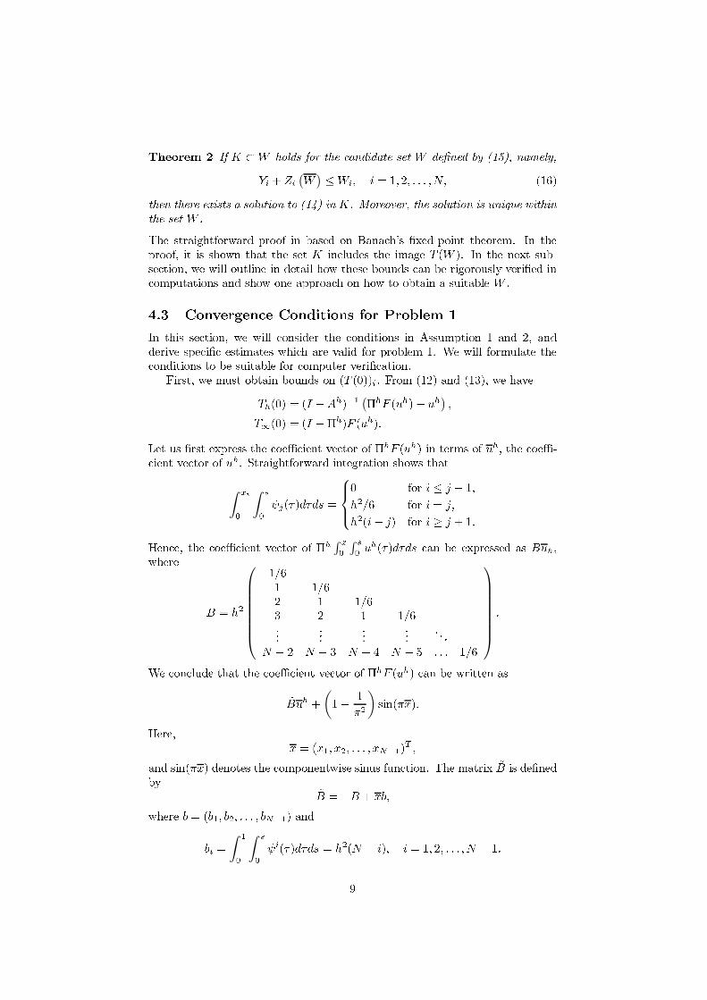

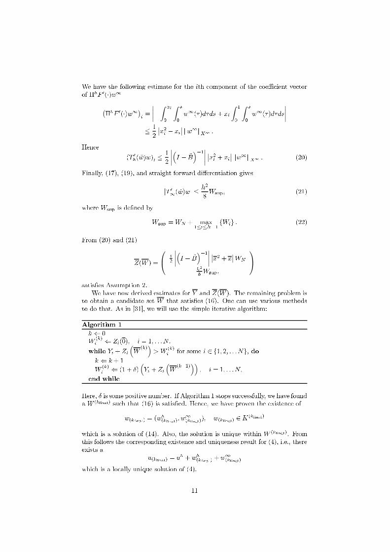


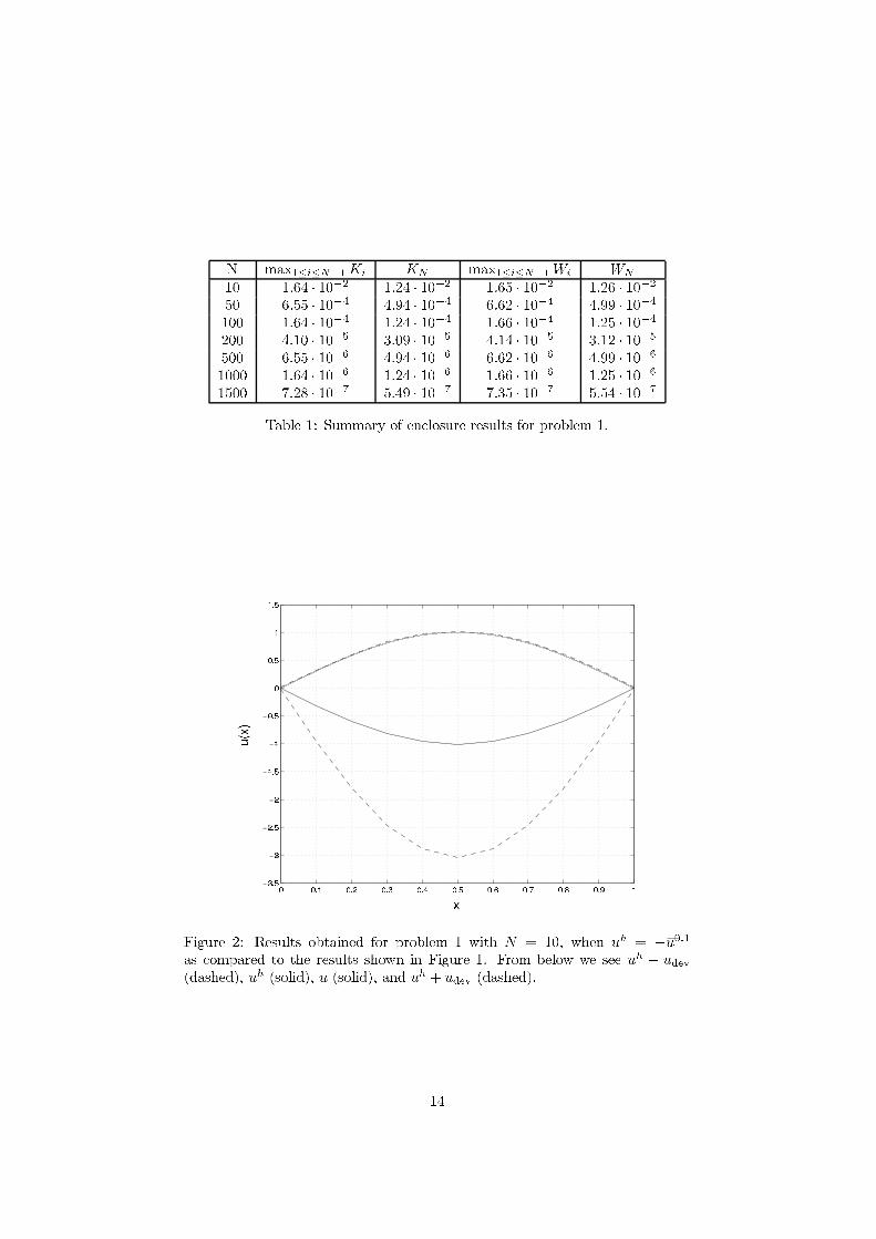


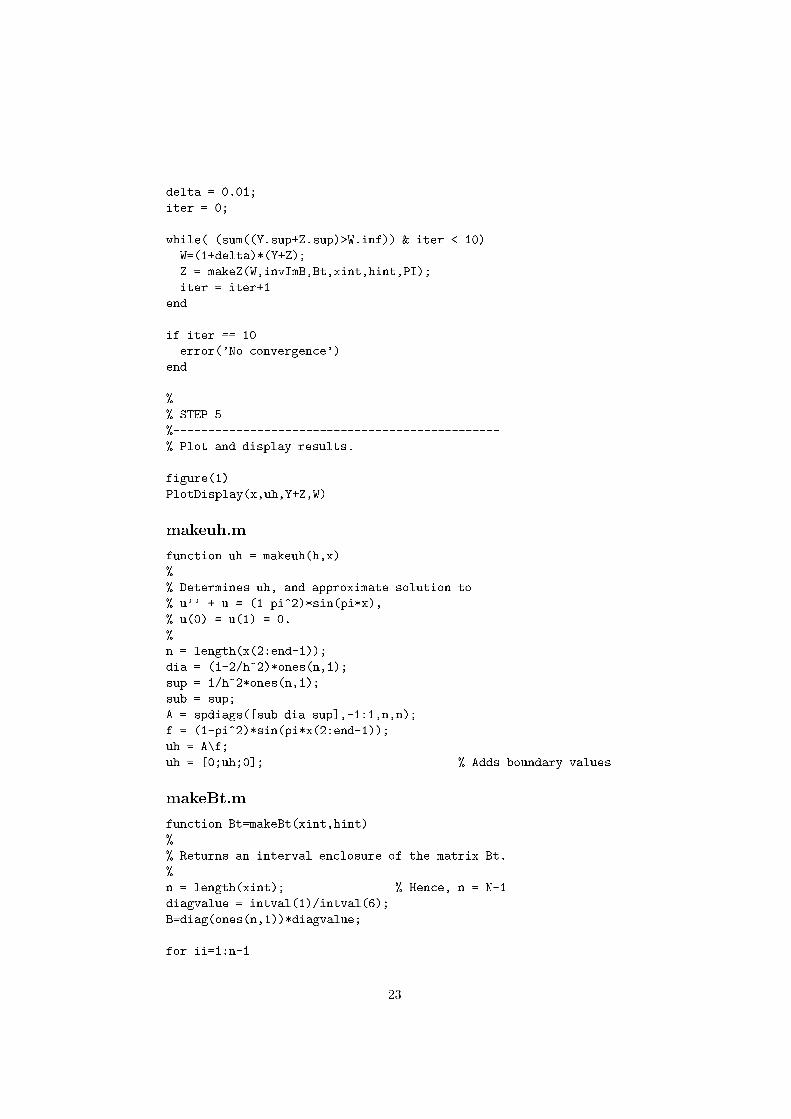


J. Fluid Mech. (2006), vol. 568, pp. 451471. c© 2006 Cambridge University Press
doi:10.1017/S0022112006002618 Printed in the United Kingdom
451
Resolvent bounds for pipe Poiseuille flow
By PER-OLOV AS EN AND GUNILLA KREISS
Department of Numerical Analysis and Computer Science, Royal Institute of Technology (KTH),S-100 44, Stockholm, Sweden
(Received 18 October 2005 and in revised form 5 June 2006)
We derive an analytical bound on the resolvent of pipe Poiseuille ow in large parts ofthe unstable half-plane. We also consider the linearized equations, Fourier transformedin axial and azimuthal directions. For certain combinations of the wavenumbers andthe Reynolds number, we derive an analytical bound on the resolvent of the Fouriertransformed problem. In particular, this bound is valid for the perturbation whichnumerical computations indicate to be the perturbation that gives the largest transientgrowth. Our bound has the same dependence on the Reynolds number as given bythe computations.
1. Introduction
Since the pioneer work on pipe ow by Reynolds in the late nineteenth century,hydrodynamical stability theory has experienced great advances. However, some of themost fundamental questions remain unanswered, such as the mechanisms responsiblefor transition to turbulence. Even in the few simple cases of shear ows wherethe analytical solutions of the NavierStokes equations are available, much is stillunknown. It has been shown that plane Couette ow is linearly stable at all Reynoldsnumbers (Romanov 1973) and that plane Poiseuille ow becomes linearly unstable atR ≈ 5772 (Orszag 1971). For pipe Poiseuille ow, laminar ow has been observed atR ≈ 105 in highly controlled experiments (Pfenninger 1961) indicating that the owis linearly stable. Also, numerous numerical computations have been done (see e.g.Lessen, Sadler & Liu 1968; Salwen, Cotton & Grosch 1980; Schmid & Henningson1994; Trefethen, Trefethen & Schmid 1999) without nding any unstable eigenvaluesof the NavierStokes equations linearized at the stationary parabolic velocity proleof pipe Poiseuille ow. However, a formal proof of linear stability exists only foraxisymmetric disturbances (Herron 1991). Hence, despite the long history of theproblem, the question of linear stability of pipe Poiseuille ow remains an openproblem.
Even more complicated and unresolved is the question of conditional nonlinearstability of pipe Poiseuille ow. Despite the believed linear stability at all Reynoldsnumbers, experiments have shown that nite-amplitude perturbations may lead toturbulence at Reynolds numbers larger than the critical Reynolds number Rc ≈ 2000(see Draad, Kuiken & Nieuwstadt 1998, and references therein). There is a thresholdfor the amplitude of the perturbation, below which the ow is stable to allperturbations. This threshold is assumed to behave as R−β , with β 1, as R → ∞(Trefethen et al. 1993). Determining the correct value of β has proved to be a challenge.Experiments and computations have indicated values in the range 1 β 3/2 (seee.g. Hof, Juel & Mullin 2003; Meseguer 2003; Shan, Zhang & Nieuwstadt 1998).By careful asymptotic analysis, Chapman (2002) argues that β = 1 and β = 3/2 for
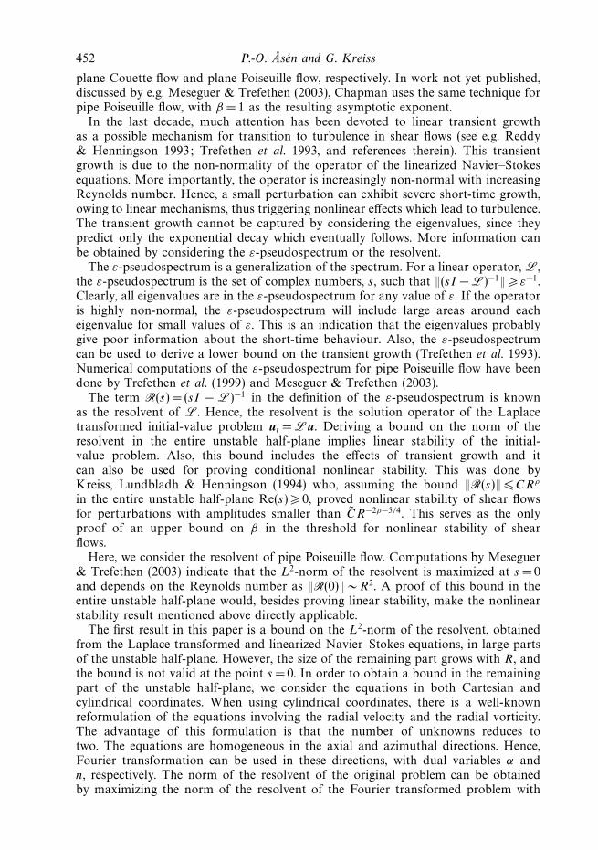
452 P.-O. Asen and G. Kreiss
plane Couette ow and plane Poiseuille ow, respectively. In work not yet published,discussed by e.g. Meseguer & Trefethen (2003), Chapman uses the same technique forpipe Poiseuille ow, with β = 1 as the resulting asymptotic exponent.
In the last decade, much attention has been devoted to linear transient growthas a possible mechanism for transition to turbulence in shear ows (see e.g. Reddy& Henningson 1993; Trefethen et al. 1993, and references therein). This transientgrowth is due to the non-normality of the operator of the linearized NavierStokesequations. More importantly, the operator is increasingly non-normal with increasingReynolds number. Hence, a small perturbation can exhibit severe short-time growth,owing to linear mechanisms, thus triggering nonlinear effects which lead to turbulence.The transient growth cannot be captured by considering the eigenvalues, since theypredict only the exponential decay which eventually follows. More information canbe obtained by considering the ε-pseudospectrum or the resolvent.
The ε-pseudospectrum is a generalization of the spectrum. For a linear operator, L,the ε-pseudospectrum is the set of complex numbers, s, such that ‖(sI − L)−1‖ ε−1.Clearly, all eigenvalues are in the ε-pseudospectrum for any value of ε. If the operatoris highly non-normal, the ε-pseudospectrum will include large areas around eacheigenvalue for small values of ε. This is an indication that the eigenvalues probablygive poor information about the short-time behaviour. Also, the ε-pseudospectrumcan be used to derive a lower bound on the transient growth (Trefethen et al. 1993).Numerical computations of the ε-pseudospectrum for pipe Poiseuille ow have beendone by Trefethen et al. (1999) and Meseguer & Trefethen (2003).
The term R(s) = (sI − L)−1 in the denition of the ε-pseudospectrum is knownas the resolvent of L. Hence, the resolvent is the solution operator of the Laplacetransformed initial-value problem ut = Lu. Deriving a bound on the norm of theresolvent in the entire unstable half-plane implies linear stability of the initial-value problem. Also, this bound includes the effects of transient growth and itcan also be used for proving conditional nonlinear stability. This was done byKreiss, Lundbladh & Henningson (1994) who, assuming the bound ‖R(s)‖ CRρ
in the entire unstable half-plane Re(s) 0, proved nonlinear stability of shear owsfor perturbations with amplitudes smaller than CR−2ρ−5/4. This serves as the onlyproof of an upper bound on β in the threshold for nonlinear stability of shearows.
Here, we consider the resolvent of pipe Poiseuille ow. Computations by Meseguer& Trefethen (2003) indicate that the L2-norm of the resolvent is maximized at s = 0and depends on the Reynolds number as ‖R(0)‖ ∼ R2. A proof of this bound in theentire unstable half-plane would, besides proving linear stability, make the nonlinearstability result mentioned above directly applicable.
The rst result in this paper is a bound on the L2-norm of the resolvent, obtainedfrom the Laplace transformed and linearized NavierStokes equations, in large partsof the unstable half-plane. However, the size of the remaining part grows with R, andthe bound is not valid at the point s =0. In order to obtain a bound in the remainingpart of the unstable half-plane, we consider the equations in both Cartesian andcylindrical coordinates. When using cylindrical coordinates, there is a well-knownreformulation of the equations involving the radial velocity and the radial vorticity.The advantage of this formulation is that the number of unknowns reduces totwo. The equations are homogeneous in the axial and azimuthal directions. Hence,Fourier transformation can be used in these directions, with dual variables α andn, respectively. The norm of the resolvent of the original problem can be obtainedby maximizing the norm of the resolvent of the Fourier transformed problem with
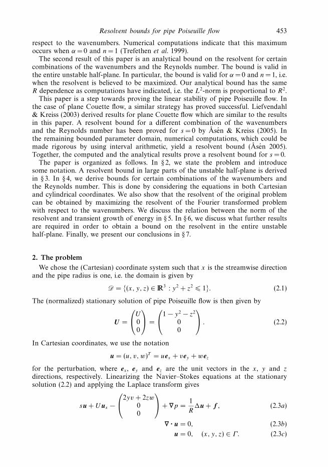
Resolvent bounds for pipe Poiseuille flow 453
respect to the wavenumbers. Numerical computations indicate that this maximumoccurs when α =0 and n= 1 (Trefethen et al. 1999).
The second result of this paper is an analytical bound on the resolvent for certaincombinations of the wavenumbers and the Reynolds number. The bound is valid inthe entire unstable half-plane. In particular, the bound is valid for α = 0 and n = 1, i.e.when the resolvent is believed to be maximized. Our analytical bound has the sameR dependence as computations have indicated, i.e. the L2-norm is proportional to R2.
This paper is a step towards proving the linear stability of pipe Poiseuille ow. Inthe case of plane Couette ow, a similar strategy has proved successful. Liefvendahl& Kreiss (2003) derived results for plane Couette ow which are similar to the resultsin this paper. A resolvent bound for a different combination of the wavenumbersand the Reynolds number has been proved for s = 0 by Asen & Kreiss (2005). Inthe remaining bounded parameter domain, numerical computations, which could bemade rigorous by using interval arithmetic, yield a resolvent bound (Asen 2005).Together, the computed and the analytical results prove a resolvent bound for s = 0.
The paper is organized as follows. In § 2, we state the problem and introducesome notation. A resolvent bound in large parts of the unstable half-plane is derivedin § 3. In § 4, we derive bounds for certain combinations of the wavenumbers andthe Reynolds number. This is done by considering the equations in both Cartesianand cylindrical coordinates. We also show that the resolvent of the original problemcan be obtained by maximizing the resolvent of the Fourier transformed problemwith respect to the wavenumbers. We discuss the relation between the norm of theresolvent and transient growth of energy in § 5. In § 6, we discuss what further resultsare required in order to obtain a bound on the resolvent in the entire unstablehalf-plane. Finally, we present our conclusions in § 7.
2. The problem
We chose the (Cartesian) coordinate system such that x is the streamwise directionand the pipe radius is one, i.e. the domain is given by
D = (x, y, z) ∈ 3 : y2 + z2
1. (2.1)
The (normalized) stationary solution of pipe Poiseuille ow is then given by
U =
U
00
=
1 − y2 − z2
00
. (2.2)
In Cartesian coordinates, we use the notation
u = (u, v, w)T = uex + vey + wez
for the perturbation, where ex , ey and ez are the unit vectors in the x, y and z
directions, respectively. Linearizing the NavierStokes equations at the stationarysolution (2.2) and applying the Laplace transform gives
su + Uux −
2yv + 2zw
00
+ ∇p =1
Ru + f , (2.3a)
∇ · u = 0, (2.3b)
u = 0, (x, y, z) ∈ Γ. (2.3c)

454 P.-O. Asen and G. Kreiss
Here, R = Uca/ν is the Reynolds number, where Uc is the centreline velocity, a thepipe radius and ν the kinematic viscosity, and Γ = (x, y, z) ∈ 3 : y2 + z2 = 1 is theboundary of D.
The resolvent, R(s), is the solution operator of (2.3ac) for a given forcing f , i.e.R(s) : f → u. We are interested in bounding the L2-norm of the resolvent in theunstable half-plane, Re(s) 0. In particular, we are interested in how the norm of theresolvent depends on the Reynolds number.
We assume that u ∈ L2 is a smooth solution, i.e. u → 0 as |x| → ∞, so that boundaryterms vanish when using integration by parts. Without any restriction, we assume∇ · f = 0 and f ∈ C∞
0 . A non-solenoidal forcing can be divided into a solenoidal partand a part affecting only the pressure (Yudovich 1989). Results for less regular forcingfollow from closure arguments. Also, since we are interested in the linear stability forlarge Reynolds numbers, we consider only R 1.
We will derive bounds on the resolvent in large parts of the unstable half-planeusing the formulation (2.3ac) and integration by parts. However, in other parts ofthe unstable half-plane, this is not possible, at least not in a straightforward way. Inthose parts, we will derive bounds for some combinations of wavenumbers and theReynolds number. The geometry of the domain suggests that cylindrical coordinatesmight be useful, and we will return to this later in the paper.
We use 〈u, v〉 and ‖u‖ = 〈u, u〉1/2 to denote the L2-inner product and L2-norm,respectively. In Cartesian coordinates, the L2-inner product is dened as
〈u, v〉 =
∫
Du · v dx.
As mentioned above, we also use cylindrical coordinates. To avoid confusion, weintroduce the corresponding equations and notation later.
3. A resolvent bound in parts of the unstable half-plane
In order to obtain a bound on the resolvent in large parts of the unstable half-plane,we consider the linearized NavierStokes equations in Cartesian coordinates, (2.3ac).First, we dene the following parts of the complex plane (see gure 1).
Σ =
s ∈ : Re(s) − 7 +1
2R|Im(s)| 0
, (3.1a)
Σ− = s /∈ Σ : Re(s) 0. (3.1b)
We can derive a bound on the resolvent using only integration by parts. The resultis summarized in the following theorem.
Theorem 3.1. If s ∈ Σ , where Σ is defined by (3.1a), then the resolvent is boundedby
‖R(s)‖ CR,
where C is a constant independent of R. Also, for s ∈ Σ we have ‖R(s)‖ → 0 as |s| → ∞.
Proof. Scalar multiply (2.3a) with u. For the term involving the pressure, we haveby using integration by parts, (2.3b) and (2.3c) so that
〈u, ∇p〉 = −〈∇ · u, p〉 = 0.
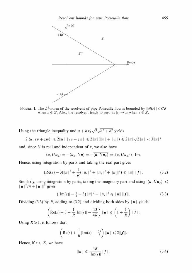
Resolvent bounds for pipe Poiseuille flow 455
Im (s)
Re (s)
Σ
Σ–
14R
–14R
Figure 1. The L2-norm of the resolvent of pipe Poiseuille ow is bounded by ‖R(s)‖ CRwhen s ∈ Σ . Also, the resolvent tends to zero as |s| → ∞ when s ∈ Σ .
Using the triangle inequality and a + b √
2√
a2 + b2 yields
2|〈u, yv + zw〉| 2‖u‖ ‖yv + zw‖ 2‖u‖(‖v‖ + ‖w‖) 2‖u‖√
2‖u‖ < 3‖u‖2
and, since U is real and independent of x, we also have
〈u, Uux〉 = −〈ux, Uu〉 = −〈u, Uux〉 ⇒ 〈u, Uux〉 ∈ Im.
Hence, using integration by parts and taking the real part gives
(Re(s) − 3)‖u‖2 +1
R(‖ux‖2 + ‖uy‖2 + ‖uz‖2) ‖u‖ ‖ f ‖. (3.2)
Similarly, using integration by parts, taking the imaginary part and using |〈u, Uux〉|
‖u‖2/4 + ‖ux‖2 gives(
|Im(s)| − 14
− 3)
‖u‖2 − ‖ux‖2 ‖u‖ ‖ f ‖. (3.3)
Dividing (3.3) by R, adding to (3.2) and dividing both sides by ‖u‖ yields(
Re(s) − 3 +1
R|Im(s)| − 13
4R
)
‖u‖
(
1 +1
R
)
‖ f ‖.
Using R 1, it follows that(
Re(s) +1
R|Im(s)| − 25
4
)
‖u‖ 2‖ f ‖.
Hence, if s ∈ Σ , we have
‖u‖ 4R
|Im(s)| ‖ f ‖. (3.4)

456 P.-O. Asen and G. Kreiss
We also have from (3.2) that
‖u‖ 1
Re(s) − 3‖ f ‖. (3.5)
Using either (3.4) or (3.5), depending on s, the result follows.
Remark. As seen from (3.5), it is enough that Re(s) > 3 (actually Re(s) > 2√
2)for the resolvent to be bounded. Hence, we could make the part of the unstable half-plane where theorem 3.1 does not hold, i.e. Σ− dened by (3.1b), somewhat smallerif desired. However, since Σ− grows as R increases, this is of minor interest. Also, theestimate (3.5) gives an R-independent bound on the resolvent when Re(s) > 3.
In order to prove linear stability and also nonlinear stability for sufficiently smallperturbations, we wish to bound the resolvent in the entire unstable half-plane. Therest of the paper is concerned with how a bound on the resolvent could also bederived in the part of the unstable half-plane not covered by theorem 3.1.
4. Resolvent bounds for certain wavenumbers
Here, we consider the Fourier transformed linearized NavierStokes equations. Wederive resolvent bounds for certain combinations of wavenumbers in relation to theReynolds number.
First, we bound the resolvent when the wavenumber in the axial direction, α, issufficiently large compared to the Reynolds number. For this, we use the linearizedNavierStokes equations in Cartesian coordinates and Fourier transformed in theaxial direction.
Next, we derive a resolvent bound when the product of the axial wavenumber, α,and the Reynolds number, R, is sufficiently small. In this case, we use the linearizedNavierStokes equations in cylindrical coordinates.
Finally, we bound the resolvent when the azimuthal wavenumber, n, is sufficientlylarge compared to the product of the axial wavenumber, α, and the Reynolds number.In this case, we use a well-known formulation involving the radial velocity and theradial vorticity.
At the end of this section, we discuss the relation between the norm of theresolvent to the original problem, (2.3ac), and the norm of the resolvent to theFourier transformed problems.
4.1. Cartesian coordinates
Since the coefficients in (2.3ac) are independent of x, we may apply the Fouriertransform, yielding
s u + iαU u −
2yv + 2zw
00
+
iαp
py
pz
=1
Ru + f , (4.1a)
iαu + vy + wz = 0, (4.1b)
u = 0, (y, z) ∈ Γ. (4.1c)
Here, =(∂2y + ∂2
z − α2) and the domain is D = (y, z) ∈ 2 : y2 + z2 1 with
boundary Γ = (y, z) ∈ 2 : y2 + z2 = 1.We dene, in analogy with the original problem, R(s, α) to be the solution operator
of (4.1ac) where α ∈ is to be considered as another parameter, i.e. R(s, α) : f → u.Note that ‖ · ‖ now denotes the L2-norm over the two-dimensional unit disk.

Resolvent bounds for pipe Poiseuille flow 457
Using integration by parts, we obtain the following lemma.
Lemma 4.1. For all α and R such that
α2 4R,
the bound
‖R(s, α)‖ 1 (4.2)
holds in the entire unstable half-plane Re(s) 0. Also, ‖R(s, α)‖ → 0 as |α| → ∞.
Proof. As in the proof of theorem 3.1, scalar multiplying (4.1a) with u, usingintegration by parts, (4.1b), (4.1c) and taking the real part gives
(Re(s) − 3)R‖u‖2 + ‖uy‖2 + ‖uz‖2 + α2‖u‖2 R‖u‖ ‖ f ‖
R
2‖u‖2 +
R
2‖ f ‖2.
Rearranging the terms and using Re(s) 0 yields
‖u‖2
(
α2 − 7R
2
)−1R
2‖ f ‖2 (4.3)
and the lemma easily follows.
4.2. Cylindrical coordinates
Here, we derive bounds when the product of the wavenumber in the axial direction,α, and the Reynolds number, R, is sufficiently small and when the wavenumber inthe azimuthal direction, n, is sufficiently large.
We use the notation
u = (u, v, w) = uex + ver + weθ
for the perturbation, where ex , er and eθ are the unit vectors in the x, r and θ
directions, respectively. The stationary solution is now given by
U =
U
00
=
1 − r2
00
.
In cylindrical coordinates, the coefficients in the linearized and Laplace transformedNavierStokes equations depend only on r . Hence, we may apply the Fouriertransform in the x and θ directions, with dual variables α and n, respectively.The resulting equations are
su + iαUu − 2rv + iαp = R−1u + f x, (4.4a)
sv + iαUv + p′ = R−1(v − r−2v − 2inr−2w) + f r , (4.4b)
sw + iαUw + r−1inp = R−1(w + 2inr−2v − r−2w) + f θ , (4.4c)
iαu + r−1(rv)′ + inr−1w = 0, (4.4d)
u = 0, r = 1, (4.4e)
where the prime denotes differentiation with respect to r . Here, the forcing isf = (f x, f r , f θ ), the domain is D = r ∈ : r ∈ [0, 1] and the Laplacian is given by
=1
r
∂
∂r
(
r∂
∂r
)
− α2 − n2
r2.

458 P.-O. Asen and G. Kreiss
We dene R(s, α, n) to be the solution operator of (4.4ae) with α and n asparameters, i.e. R(s, α, n) : f → u. Clearly, u is periodic in the azimuthal direction.Hence, n only takes integer values, i.e. n ∈ , and, as before, α ∈.
The only remaining space dimension is r , and since we use cylindrical coordinates,the scalar product is given by
u, v= ∫ 1
0
u · vr dr. (4.5)
In this section,denotes the norm induced by (4.5), i.e. over the one-dimensionaldomain r ∈ [0, 1]. Using Parsevals formula, this norm can be related to the L2-normover the unit disk and to the L2-norm over the entire three-dimensional domain (2.1).This is discussed in4.3.
We rst consider axisymmetric perturbations, i.e. n = 0, in which case we derive thefollowing lemma.
Lemma 4.2. When n = 0 andαR 1/16, the boundR(s, α, 0) CR
holds in the entire unstable half-plane, Re(s) 0. Here, C is a constant independent ofα and R.
Proof. First, with the scalar product (4.5) we have by using (4.4d), (4.4e) and n = 0that
u, iαp+v, p′=−iαu + r−1(rv)′, p= 0,
iα(u, Uu+v, Uv+w, Uw) ∈ Im.
Note that the boundary term from the integration by parts vanishes by using (4.4e)at r = 1 and by using that v, p are bounded at r =0, i.e. vprr=0 = 0. In the rest ofthis proof, we use (4.4e) and the fact that u and u′ are bounded at r = 0 in order toremove boundary terms appearing when using integration by parts.
Now, scalar multiplying (4.4a) with u, (4.4b) with v and (4.4c) with w, usingintegration by parts, taking the real part and adding the resulting equations yields
(Re(Rs) + α2)u2 +u′2 +r−1v2 +r−1w2 Ruf x+ Rvf r+ Rwf θ+2R
u, rv
14u2 + 2R2f2 +2R
u, rv. (4.6)
For the last term on the right-hand side, we required the inequalityru∞ 2u+u′, (4.7)
where∞ denotes the L∞−norm. In order to prove (4.7), note that since u iscontinuous, there exist rm and rM such thatrmu(rm)= min
r∈[0,1]ru(r)ruu, rM u(rM )= max
r∈[0,1]ru(r)=ru∞.
Now, (4.7) follows fromrM u(rM )2−rmu(rm)2 =
∫ rM
rm
(r2u2)′ dr =
∫ rM
rm
2ru2 + 2r2uu′ dr
2u2 + 2uu′ 3u2 +u′2and (4u2 +u′2)1/2 2u+u′.

Resolvent bounds for pipe Poiseuille flow 459
With n = 0 we have, from (4.4d), (rv)′ = − iαur or rv = − iα∫ r
0us ds. Using this
and (4.7) yields2Ru, rv= 2R
∣
∣
∣
∣
∫ 1
0
u
(
iα
∫ r
0
us ds
)
r dr
∣
∣
∣
∣
2αRru∞
∫ 1
0
ur2 dr
2αR(2u+u′) (∫ 1
0
u2r dr
)1/2 (∫ 1
0
r3 dr
)1/2
= 2αR(2u+u′)u1
2αR(
3u2 + 14u′2). (4.8)
We also need the Poincare type inequalityu2 14u′2. (4.9)
Consider one component of u, e.g. u. Using u= −∫ 1
ru′ds yieldsu2 =
∫ 1
0
[∫ 1
r
u′ ds
]2
r dr
∫ 1
0
[
(∫ 1
r
u′2s ds
)1/2 (∫ 1
r
s−1 ds
)1/2]2
r dr
u′2 ∫ 1
0
ln(r)r dr = 1
4u′2.
Doing the same for v and w gives (4.9).From (4.6), (4.8) and (4.9) we have, using Re(Rs) 0,
(
α2 + 34
− 3αR)u2 +
(
34
− 14
αR)u′2 2R2f2.
The conditionαR 1/16 is more than enough to ensure that the term in parentheses
on the left-hand side is positive, and the lemma follows.
In order to obtain a resolvent bound when the azimuthal wavenumber, n, issufficiently large, we consider a well-known reformulation of the problem. Thisformulation is obtained by eliminating the pressure and formulating equations for theradial velocity, v, and the radial vorticity, η (Burridge & Drazin 1969). The resultingequations are
1
RT2Φ − (iαU + s)TΦ + k2iαr
(
U ′
k2r
)′Φ − 2αn
RTΩ = −Tξ, (4.10a)
1
RSΩ − (iαU + s)Ω +
2αn
Rk4r4TΦ +
inU ′
k2r3Φ = −χ. (4.10b)
Here, the prime denotes differentiation with respect to r , k2 =α2 + n2/r2 and
Φ = −irv, Ω =αrw − nu
k2r2=
−η
ik2r,
ξ = −irf r , χ =αrf θ − nf x
k2r2,
T = k2r∂
∂r
(
1
k2r
∂
∂r
)
− k2, S =1
k2r3
∂
∂r
(
k2r3 ∂
∂r
)
− k2. (4.11a,b)

460 P.-O. Asen and G. Kreiss
The corresponding boundary conditions are given by (see e.g. Schmid & Henningson2001),
r = 1: Φ = Φ ′ = Ω = 0,
r = 0, n = 0: Φ = Φ ′ = 0,
r = 0,n= 1: Φ = Ω = 0, Φ ′ nite,r = 0,n 2: Φ = Φ ′ = Ω = 0.
(4.12)
The two variables Φ and Ω completely describe the system. The original variablescan be recovered from
u = − α
k2rΦ ′ − nΩ, v =
iΦ
r, w = − n
k2r2Φ ′ + αrΩ.
Hence, the L2-norm can be computed as u 2 = r−1Φ 2 + k−1r−1Φ ′ 2 + krΩ 2, (4.13)
and similarly,
f 2 can be computed as
f 2 = r−1ξ 2 + k−1r−1ξ ′ 2 + krχ 2.
Using (4.10a, b), we obtain the following lemma.
Lemma 4.3. For all α, n and R such that
n2 16αR,
the bound R(s, α, n)
CR2
holds in the entire unstable half-plane, Re(s) 0. Here, C is a constant independent ofα, n and R. Also, for any fixed α and R,
R(s, α, n) →0 asn→∞.
Proof. The rather lengthy proof is given in the Appendix.
4.3. The relation between the original problem and the Fourier transformed problems
Here, we discuss how the bounds on R(s, α)
and R(s, α, n)
can be used to derivea bound on R
(s) . The arguments closely follow those used by Liefvendahl & Kreiss
(2003). We start by proving the following theorem.
Theorem 4.2. For all α, n and R such that at least one of the inequalitiesαR 116
, α3 4αR, n2 16αR (4.14ac)
hold, there is a constant C, independent of α, n, R and Re(s) 0, such that R(s, α, n)
CR2. (4.15)
Also, R(s, α, n) →0 asα+n→∞.
Proof. Lemma 4.3 gives (4.15) when (4.14c) holds. Also, using lemma 4.3 whenn = 0 and lemma 4.2 when n = 0 yields (4.15) when (4.14a) holds. Proving thatlemma 4.1 is also valid for R(s, α, n) for any value of n will give (4.15) when (4.14b)holds, and will thus be the equivalent of proving the theorem.
When we derived lemma 4.1, we used the linearized NavierStokes equations inCartesian coordinates, Fourier transformed in the axial direction. Clearly, the L2-
norm over the unit disk of u and f is the same when using cylindrical coordinates as
when using Cartesian coordinates. Hence, we may assume that R(s, α) in lemma 4.1is the solution operator of the once Fourier transformed problem given in cylindricalcoordinates.
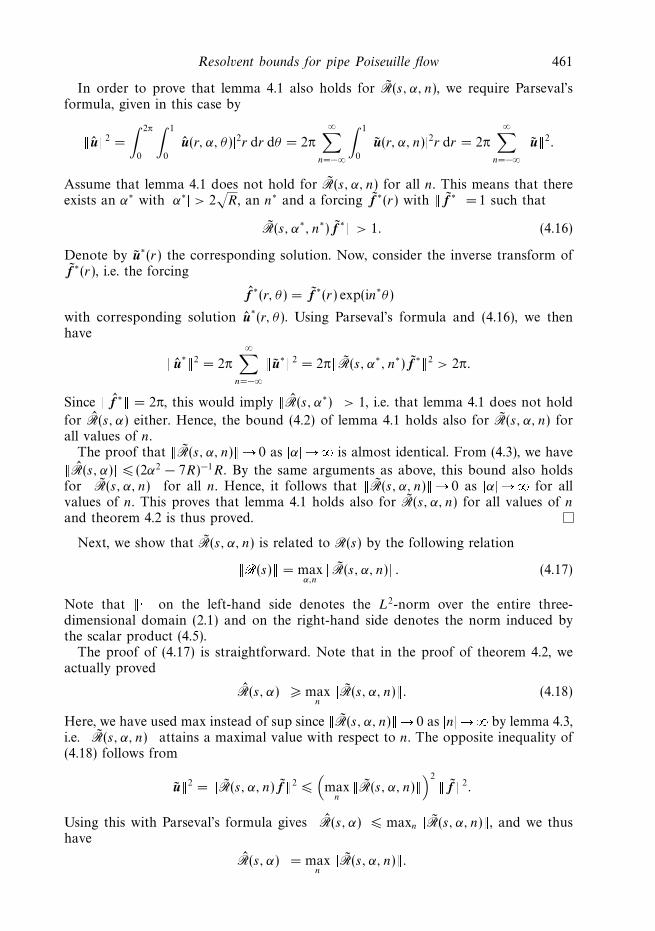
Resolvent bounds for pipe Poiseuille flow 461
In order to prove that lemma 4.1 also holds for R(s, α, n), we require Parsevalsformula, given in this case by
u2 =
∫ 2π
0
∫ 1
0
u(r, α, θ)2r dr dθ = 2π
∞∑
n=−∞
∫ 1
0
u(r, α, n)2r dr = 2π
∞∑
n=−∞
u2.
Assume that lemma 4.1 does not hold for R(s, α, n) for all n. This means that thereexists an α∗ withα∗> 2
√R, an n∗ and a forcing f ∗(r) with
f ∗= 1 such thatR(s, α∗, n∗) f ∗> 1. (4.16)
Denote by u∗(r) the corresponding solution. Now, consider the inverse transform off ∗(r), i.e. the forcing
f ∗(r, θ) = f ∗(r) exp(in∗θ)
with corresponding solution u∗(r, θ). Using Parsevals formula and (4.16), we then
have u
∗2 = 2π
∞∑
n=−∞
u∗2 = 2π
R(s, α∗, n∗) f ∗2 > 2π.
Since
f ∗= 2π, this would implyR(s, α∗)
> 1, i.e. that lemma 4.1 does not hold
for R(s, α) either. Hence, the bound (4.2) of lemma 4.1 holds also for R(s, α, n) forall values of n.
The proof thatR(s, α, n)→0 asα→∞is almost identical. From (4.3), we haveR(s, α)
(2α2 − 7R)−1R. By the same arguments as above, this bound also holds
forR(s, α, n)
for all n. Hence, it follows thatR(s, α, n)→0 asα→∞for all
values of n. This proves that lemma 4.1 holds also for R(s, α, n) for all values of n
and theorem 4.2 is thus proved.
Next, we show that R(s, α, n) is related to R(s) by the following relationR(s)= max
α,n
R(s, α, n). (4.17)
Note thaton the left-hand side denotes the L2-norm over the entire three-
dimensional domain (2.1) and on the right-hand side denotes the norm induced bythe scalar product (4.5).
The proof of (4.17) is straightforward. Note that in the proof of theorem 4.2, weactually proved R(s, α)
max
n
R(s, α, n). (4.18)
Here, we have used max instead of sup sinceR(s, α, n)→0 asn→∞by lemma 4.3,
i.e.R(s, α, n)
attains a maximal value with respect to n. The opposite inequality of(4.18) follows from
u2 =R(s, α, n) f2
(
maxn
R(s, α, n))2
f2.
Using this with Parsevals formula givesR(s, α)
maxn
R(s, α, n), and we thus
have R(s, α)= max
n
R(s, α, n).
462 P.-O. Asen and G. Kreiss
In order to prove (4.17), we must now prove
‖R(s)‖ = maxα
‖R(s, α)‖. (4.19)
For this, we require ‖R(s, α)‖ → 0 as |α| → ∞, in order to ensure that ‖R(s, α)‖ attainsa maximal value with respect to α; but this follows from lemma 4.1. Now, the rest ofthe proof is similar to the proof above, although some care must be taken becauseα ∈ , i.e. α does not only take integer values as n does. The proof of (4.19) wasdone by Liefvendahl & Kreiss (2003) and (4.17) follows.
5. Relation between the resolvent and transient growth
For pipe Poiseuille ow, numerical computations concerning the energy of an initialperturbation as a function of time have been done by e.g. Schmid & Henningson(1994) and Meseguer & Trefethen (2003). The results show that a substantial initialgrowth of energy is possible despite the stable eigenvalues. In this section, we relatethe norm of the resolvent to this transient growth of energy.
Consider the initial-value problem
ut = Lu, (5.1a)
u(0) = u0, (5.1b)
where L is a linear operator independent of time. If we denote the solution operatorof (5.1ab) by etL, we have
u(t) = etLu0. (5.2)
Since ‖u(t)‖ ‖etL‖ ‖u0‖, we may use ‖etL‖ as a measure of the largest possiblegrowth (in the norm used) as a function of time. In hydrodynamic stability, theL2-norm is typically used, since the square of the L2-norm can be interpreted as anenergy.
Assume that the spectrum of L is in the left half-plane, i.e. limt → ∞ ‖u(t)‖ = 0.Clearly, this implies limt → ∞ ‖etL‖ = 0. Now, if L is a normal operator, we have‖etL‖ 1, ∀t 0. This means that no growth of the norm of the solution is possiblefor any initial data, u0. However, if L is non-normal, the norm of the solution canexperience an initial growth, i.e. ‖etL‖ > 1 for some times t > 0, before eventuallydecaying.
In order to derive a relation between the resolvent and the solution operator, etL,we apply the Laplace transform to (5.1a). The solution can then be written as
u(s) = (sI − L)−1u0 ≡ R(s)u0, (5.3)
where I is the identity operator and R(s) = (sI − L)−1 is the resolvent of L.Applying the Laplace transform to (5.2) and comparing with (5.3), we nd from
the denition of the Laplace transform that
R(s) =
∫ ∞
0
e−stetL dt. (5.4)
If ‖etL‖ is large, one also expects the norm of the resolvent to be large. Note thatthe resolvent integrates the effects of transient growth over time. Thus, the norm ofthe resolvent can be signicantly larger than ‖etL‖.
The effects of transient growth can be illustrated by a simple example taken fromSchmid & Henningson (1994), and we refer to this paper for further details. Consider

Resolvent bounds for pipe Poiseuille flow 463
the 2 × 2 model problem (5.1) for u = (u, v)T and L given by
L =
(
−1/R 01 −2/R
)
. (5.5)
Clearly, the eigenvalues of L are in the left-hand half-plane for all R > 0. Thesolution operator of this model problem is
etL =
(
e−t/R 0−
(
e−2t/R − e−t/R)
R e−2t/R
)
.
From this, we see that supt0etL∼R and that the maximum is attained at a timet ∼ R. Hence, we expect the norm of the resolvent to be proportional to R2.
The resolvent of (5.5) is given by
R(s) = (sI − L)−1 =
R
sR + 10
R2
(sR + 1)(sR + 2)
R
sR + 2
. (5.6)
It follows thatR(0)∼R2, which is what we expected frometL.For pipe Poiseuille ow, numerical computations by Schmid & Henningson (1994)
indicate that a perturbation with α =0 and n =1 gives the largest transient growth.For this perturbation, the numerical results of both Schmid & Henningson (1994)and Meseguer & Trefethen (2003) are
supt>0etLL2 ∼ R,
with the maximum occurring at a time t ∼ R. We may thus expect the L2-norm ofthe resolvent (at least at s = 0) to be proportional to R2, which is conrmed by theextensive numerical computations of Meseguer & Trefethen (2003). Thus, it is likelythat for this perturbation, i.e. for α = 0 and n= 1, our resolvent bound in theorem 4.2is sharp.
For further results relating the transient growth to the ε-pseudospectrum and theresolvent, see Reddy, Schmid & Henningson (1993) and Trefethen et al. (1993).
6. Discussion
In4, we derived bounds on the resolvent for certain combinations of thewavenumbers and the Reynolds number. We also showed how these results canbe used to give a bound on the resolvent of the original problem by using (4.17).Here, we discuss what further results are required to obtain a rigorous bound on theresolvent in the entire unstable half-plane.
By theorem 3.1, we already have a bound on the resolvent when s ∈ Σ . In theremaining part of the unstable half-plane, Σ− dened by (3.1b), we would like to use(4.17) to obtain a bound.
The resolvent of the Fourier transformed problem depends on four parameters, α,n, R and s. For convenience, we choose instead the parameters α, n, αR and sR. Wewould thus like to boundR(s, α, n)in the parameter domain
Υ =α, αR ∈ , n ∈ , sR ∈ .The bound should be valid at least for all s ∈ Σ−, i.e. we may assume Re(s) 7,s CR etc. if needed.

464 P.-O. Asen and G. Kreiss
Deriving an analytical bound on the resolvent in the entire parameter domain, Υ ,would probably be extremely complicated. Instead, assume that for s ∈ Σ−, we couldprove that there is some large constant C such thatR(s, α, n)is bounded when
sR+αR C2. (6.1)
Using theorem 4.2, it would be sufficient if the proof were valid forα3 4αR.
Since, by theorem 4.2, we already have a bound whenαR n2/16, this would
imply a bound also whenn 4C for all values of α, αR and sR. Also, since we
assume R 1, (6.1) holds whenα C2. Hence, in order to cover the entire parameter
domain, Υ , it would be sufficient to obtain bounds in the parameter domain
Υ − = α∈[0, C2],αR∈
[1/16, C2],n∈
[0, 4C] ∩ ,sR∈
[0, C2]".This is a bounded parameter domain which opens for the possibility of using rigorousnumerical computations to cover it. These computations would have to be combinedwith analytical results, since Υ − still contains an innite number of parameter values.
The analytical results should be such that if a numerical bound on the resolventis valid at a point (α∗, αR∗, n∗, sR∗) ∈ Υ −, a bound follows in some neighbourhoodof this point. That is, given the numerical bound, an analytical bound follows forall combinations of α, αR, n and sR such that g(α, αR, n, sR) ε, where g is acontinuous function with g(α∗, αR∗, n∗, sR∗) = 0. The value of ε could depend on thepoint chosen, but should be explicitly computable. Also, note that all computationswould have to be done with rigorous numerical methods using interval arithmetic.
For plane Couette ow, a resolvent bound has been derived under a conditionsimilar to (6.1) at the point s = 0 (Asen & Kreiss 2005). The remaining parameterdomain is bounded. Analytical results of the type described above were derived byAsen (2005), making it possible to prove a rigorous bound on the resolvent at thepoint s = 0 in the unstable half-plane.
Remark. Numerical computations by Schmid & Henningson (1994) indicate thatwhen n = 0, the transient growth decreases with increasing αR. Also, computationsby Meseguer & Trefethen (2003) suggest that the resolvent is maximized at s =0.This indicates that a resolvent bound could be derived analytically when (6.1) holds,if C is chosen large enough.
Remark 2. The results derived in this paper can easily be improved; Σ− can bemade smaller and theorem 4.2 can cover a larger parameter domain. In order to keepthe technicalities at a minimum, we have not aimed at making the results as sharp aspossible. However, if the desired analytical results discussed in this section are derivedand rigorous numerical computations are to be used in a bounded parameter domain,making the results as sharp as possible could be important in order to reduce theamount of computation required.
7. Conclusions
In this paper, we derive bounds on the resolvent of pipe Poiseuille ow. In alarge part of the unstable half-plane, a bound is obtained by using integration byparts, see theorem 3.1. However, the size of the remaining part increases with incre-asing Reynolds number. Also, the theorem does not cover the point s =0, which iswhere numerical computations indicate that the resolvent is maximized (Meseguer &Trefethen 2003).

Resolvent bounds for pipe Poiseuille flow 465
In order to obtain a bound on the resolvent in the remaining part of the unstablehalf-plane, we consider the linearized NavierStokes equations, Fourier transformedin the axial and azimuthal directions. We show, as was done by Liefvendahl &Kreiss (2003), that the norm of the resolvent of the original problem is obtainedby maximizing the norm of the resolvent of the Fourier transformed problem withrespect to the two wavenumbers, α and n.
We derive bounds on the norm of the resolvent for different combinations ofthe axial wavenumber, α, the azimuthal wavenumber, n, and the Reynolds number,R. The results are presented in theorem 4.2. In particular, the theorem is valid forperturbations with α = 0 and n = 1, which from numerical computations is believedto yield the largest transient growth (Schmid & Henningson 1994) and the largestresolvent (Trefethen et al. 1999). Also, our resolvent bound, ‖R(s, α, n)‖ CR2, hasthe same dependence on the Reynolds number as the results from the numericalcomputations.
The conditions (4.14ac) of theorem 4.2 include perturbations of different physicalproperties. For instance, structures with weak streamwise dependency are covered by(4.14a) or (4.14c). The velocity eld of the perturbation that gives the largest transientgrowth, determined by Schmid & Henningson (1994), is of this type. It consists oftwo counter-rotating vortices near the centre of the pipe. Further, (4.14b) is valid forperturbations with large axial wavenumber compared to the Reynolds number, i.e.for perturbations which are severely affected by viscosity.
The remaining parameter domain for α, n, R and s is still unbounded. We brieydiscuss what further results are required in order to obtain a bounded parameterdomain. Under the conditions for deriving such a result, we also discuss how rigorousnumerical computations could be used to obtain a bound on the resolvent in theremaining bounded parameter domain. This would result in a bound on the resolventin the entire unstable half-plane, which would also serve as the rst proof of linearstability of pipe Poiseuille ow.
Part of this work was done while visiting Professor Peter Schmid at the Universityof Washington, Seattle, USA, and we are thankful for his help and comments on thesubject. The work was supported by Swedish Research Council grant 2003-5443.
Appendix. Proof of lemma 4.3
We will use (4.10a,b) and integration by parts to prove lemma 4.3. More precisely,we will show that there is a constant C independent of α, n and R, such that
‖r−1Φ‖2 + ‖k−1r−1Φ ′‖2 + ‖krΩ‖2
CR4
n2(‖r−1ξ‖2 + ‖k−1r−1ξ ′‖2 + ‖krχ‖2) (A 1)
holds when n2 16|αR|. Here, ‖ · ‖ is the norm induced by the scalar product(4.5). The bound ‖R(s, α, n)‖ CR2 then follows from (4.13). Also, this proves that‖R(s, α, n)‖ → 0 as |n| → ∞ and the lemma is proved.
When n = 0, the lemma is valid only for α = 0. In this case, lemma 4.2 gives thedesired resolvent bound. Thus, we assume |n| 1 in the remainder of the proof.
We use a prime to denote differentiation with respect to r . Although we use onlyintegration by parts, the r appearing in the scalar product (4.5) makes the proofsomewhat technical. Also, since r appears in the denominator at several places in theequations, the boundary terms appearing from using integration by parts must behandled with care.

466 P.-O. Asen and G. Kreiss
First, we multiply (4.10a) with k−2r−2R, scalar multiply with Φ and take the realpart. Note that
⟨
Φ,k2iαrR
k2r2
(
U ′
k2r
)′Φ
⟩
∈ Im
and, using integration by parts and the boundary conditions (4.12),
Re
(
−⟨
Φ,sR
k2r2TΦ
⟩)
= Re(sR)(#r−1Φ#2 +#k−1r−1Φ ′#2).Since Re(Rs) 0, we thus have
Re
(⟨
Φ,1
k2r2T2Φ
⟩)
∣
∣
∣
∣
Re
(⟨
Φ,iαUR
k2r2TΦ
⟩)∣
∣
∣
∣
+
∣
∣
∣
∣
Re
(⟨
Φ,2αn
k2r2TΩ
⟩)∣
∣
∣
∣
+
∣
∣
∣
∣
Re
(⟨
Φ,R
k2r2Tξ
⟩)∣
∣
∣
∣
. (A 2)
Using integration by parts, we will derive a lower bound on the term on the left-handside of (A 2) and upper bounds on the terms on the right-hand side of (A 2). Usingthe denition of T (4.11a), we have
⟨
Φ,1
k2r2T2Φ
⟩
=
∫ 1
0
Φ
(
1
k2r(TΦ)′
)′dr −
⟨
Φ,1
r2TΦ
⟩
. (A 3)
The integral is rewritten, using integration by parts, as
∫ 1
0
Φ
(
1
k2r(TΦ)′
)′dr =
[
Φ1
k2r(TΦ)′
]r=1
r=0
−∫ 1
0
Φ′ 1
k2r(TΦ)′ dr
=
[
Φ1
k2r(TΦ)′ − Φ
′ 1
k2rTΦ
]r=1
r=0
+
∫ 1
0
(
Φ′′ 1
k2r+ Φ
′(
1
k2r
)′)
TΦ dr. (A 4)
From the denition of T, (4.11a), we have
1
krTΦ =
1
krΦ ′′ + k
(
1
k2r
)′Φ ′ − k
rΦ.
Using this, the integral on the right-hand side of (A 4) can be written as
∫ 1
0
(
Φ′′ 1
k2r+ Φ
′(
1
k2r
)′)
TΦ dr =
∫ 1
0
(
1
krTΦ +
k
rΦ
)
1
krTΦr dr
=#k−1r−1TΦ#2 +
⟨
Φ,1
r2TΦ
⟩
. (A 5)
It follows from (A 3), (A 4) and (A 5) that
⟨
Φ,1
k2r2T2Φ
⟩
=#k−1r−1TΦ#2 +
[
Φ1
k2r(TΦ)′ − Φ
′ 1
k2rTΦ
]r=1
r=0
. (A 6)
We have kept the boundary terms which appear from using integration by parts,since it is not obvious that they are zero or even that they are bounded. We will nowshow that the boundary terms are zero.
Resolvent bounds for pipe Poiseuille flow 467
Expanding the boundary terms in (A 6) gives
Φ1
k2r(TΦ)′ − Φ
′ 1
k2rTΦ =
2n2ΦΦ
k2r4− ΦΦ ′
r+
4n4ΦΦ ′
k6r7− 6n2ΦΦ ′
k4r5+
ΦΦ ′
k2r3
+2n2ΦΦ ′′
k4r4− ΦΦ ′′
k2r2+
ΦΦ ′′′
k2r+
Φ′Φ
r− 2n2Φ
′Φ ′
k4r4+
Φ′Φ ′
k2r2− Φ
′Φ ′′
k2r.
At r = 1 we have the boundary condition, (4.12), Φ = Φ ′ = 0 and all terms above arethus zero at r = 1. At r =0, we have for$n$=1 that Φ = 0 and Φ ′ < ∞ and for$n$ 2that Φ = Φ ′ = 0. Also, since n%= 0, k−ar−b$r=0 is bounded if a = b and zero if a > b.Hence, the remaining terms as r → 0 are
Φ1
k2r(TΦ)′ − Φ
′ 1
k2rTΦ
∣
∣
∣
∣
r→0
=2n2ΦΦ
k2r4− ΦΦ ′
r+
4n4ΦΦ ′
k6r7− 6n2ΦΦ ′
k4r5+
ΦΦ ′
k2r3
+Φ
′Φ
r− 2n2Φ
′Φ ′
k4r4+
Φ′Φ ′
k2r2
∣
∣
∣
∣
∣
r→0
. (A 7)
At r = 0 we have byl'Hospital'srule and the boundary conditions that
Φ′Φ
r− ΦΦ ′
r
∣
∣
∣
∣
∣
r→0
=Φ
′′Φ + Φ
′Φ ′ − Φ
′Φ ′ − ΦΦ ′′
1
∣
∣
∣
∣
∣
r→0
= 0. (A 8)
Again, usingl'Hospital'srule, k′ = − n2k−1r−3 and kara$r=0 = na , we have (below, weassume r → 0 in all expressions)
2n2ΦΦ
k2r4= 2n2 Φ
′Φ + ΦΦ ′
4k2r3 − 2n2r= 2n2 Φ
′′Φ + 2Φ
′Φ ′ + ΦΦ ′′
4(3k2r2 − 2n2) − 2n2= 2Φ
′Φ ′
∣
∣
∣
r=0, (A 9a)
4n4ΦΦ ′
k6r7= 4n4 Φ
′Φ ′ + ΦΦ ′′
7k6r6 − 6n2k4r4= 4
Φ′Φ ′
n2
∣
∣
∣
∣
∣
r=0
, (A 9b)
−6n2ΦΦ ′
k4r5= −6n2 Φ
′Φ ′ + ΦΦ ′′
5k4r4 − 4n2k2r2= −6
Φ′Φ ′
n2
∣
∣
∣
∣
∣
r=0
, (A 9c)
ΦΦ ′
k2r3=
Φ′Φ ′ + ΦΦ ′′
3k2r2 − 2n2=
Φ′Φ ′
n2
∣
∣
∣
∣
∣
r=0
, (A 9d)
−2n2Φ′Φ ′
k4r4= −2
Φ′Φ ′
n2
∣
∣
∣
∣
∣
r=0
, (A 9e)
Φ′Φ ′
r2k2=
Φ′Φ ′
n2
∣
∣
∣
∣
∣
r=0
. (A 9f)
Hence, from (A 7), (A 8) and (A 9a/f), it follows that
Φ1
k2r(TΦ)′ − Φ
′ 1
k2rTΦ
∣
∣
∣
∣
r→0
= 2
(
1 − 1
n2
)
Φ′Φ ′$r=0 = 0,
where in the last step we use 1 − n−2 =0 if$n$=1 and Φ ′$r =0 = 0 if$n$ 2. We havethus shown that the boundary terms in (A 6) are zero, and it follows that
Φ,1
k2r2T2Φ =1k−1r−1TΦ12. (A 10)

468 P.-O. Asen and G. Kreiss
We will now use integration by parts to derive an expression involving the desiredterms ‖r−1Φ‖ and ‖k−1r−1Φ ′‖ which appear on the left-hand side of (A 1). First, notethat since maxr∈[0,1] n
2/k2 1, we have
n2‖k−2r−1TΦ‖2 ‖k−1r−1TΦ‖2. (A 11)
From the de3nition of T (4.11a), we have
‖k−2r−1TΦ‖2 =
∫ 1
0
((
1
k2rΦ
′)′
−1
rΦ
)((
1
k2rΦ ′
)′
−1
rΦ
)
r dr
= ‖r−1Φ‖2 + ‖(k−2r−1Φ ′)′‖2
−
∫ 1
0
Φ
(
1
k2rΦ ′
)′
dr −
∫ 1
0
Φ
(
1
k2rΦ
′)′
dr. (A 12)
Using integration by parts and the boundary conditions gives
−
∫ 1
0
Φ
(
1
k2rΦ ′
)′
dr = −
[
Φ1
k2rΦ ′
]r=1
r=0
+
∫ 1
0
Φ′ 1
k2r2Φ ′r dr = ‖k−1r−1Φ ′‖2. (A 13)
Thus, using (A 10), (A 11), (A 12) and (A 13), we have the following lower bound onthe term on the left-hand side of (A 2).
Re
⟨
Φ,1
k2r2T2Φ
⟩
n2(
‖r−1Φ‖2 + 2‖k−1r−1Φ ′‖2 + ‖(k−2r−1Φ ′)′‖2)
. (A 14)
For the3rstterm on the right-hand side of (A 2), integration by parts yields
⟨
Φ,iαU
k2r2TΦ
⟩
=
∫ 1
0
Φiα(1 − r2)
(
1
r
(
1
k2rΦ ′
)′
−1
r2Φ
)
r dr
= iα(‖Φ‖2 − ‖r−1Φ‖2) +
[
Φiα(1 − r2)1
k2rΦ ′
]r=1
r=0
− iα
∫ 1
0
(
Φ′(1 − r2) − Φ2r
) 1
k2rΦ ′ dr
= iα(‖Φ‖2 − ‖r−1Φ‖2 + ‖k−1Φ ′‖2 − ‖k−1r−1Φ ′‖2)
+ 2iα
∫ 1
0
Φ
r
Φ ′
kr
r
kr dr.
Since maxr∈[0,1] r/k 1/|n|, this gives∣
∣
∣
∣
Re
(⟨
Φ,iαUR
k2r2TΦ
⟩)∣
∣
∣
∣
2|αR|
|n|‖r−1Φ‖ ‖k−1r−1Φ ′‖. (A 15)
Similarly, using integration by parts, the following results for the other terms in(A 2) are easily obtained
∣
∣
∣
∣
Re
⟨
Φ,2αn
k2r2TΩ
⟩∣
∣
∣
∣
2|α|
|n|(‖r−1Φ‖ ‖k2rΩ‖ + ‖k−1r−1Φ ′‖ ‖krΩ ′‖), (A 16a)
∣
∣
∣
∣
Re
⟨
Φ,R
k2r2Tξ
⟩∣
∣
∣
∣
R(‖r−1Φ‖ ‖r−1ξ‖ + ‖k−1r−1Φ ′‖ ‖k−1r−1ξ ′‖). (A 16b)
Resolvent bounds for pipe Poiseuille flow 469
Hence, using (A 14), (A 15) and (A 16a,b) in (A 2) yields
n2(‖r−1Φ‖2 + 2‖k−1r−1Φ ′‖2) 2|αR|
|n|‖r−1Φ‖ ‖k−1r−1Φ ′‖
+2|α|
|n|(‖r−1Φ‖ ‖k2rΩ‖ + ‖k−1r−1Φ ′‖ ‖krΩ ′‖)
+ R(‖r−1Φ‖ ‖r−1ξ‖ + ‖k−1r−1Φ ′‖ ‖k−1r−1ξ ′‖).
Using ab a2/(2ε) + εb2/2, valid for ε > 0, on the right-hand side gives
n2(‖r−1Φ‖2 + 2‖k−1r−1Φ ′‖2) 2|αR|
|n|3n2
(
14‖r−1Φ‖2 + ‖k−1r−1Φ ′‖2
)
+n2
4‖r−1Φ‖2
+4α2
n4‖k2rΩ‖2 +
n2
2‖k−1r−1Φ ′‖2 +
2α2
n4‖krΩ ′‖2
+n2
8(‖r−1Φ‖2 + ‖k−1r−1Φ ′‖2)
+2R2
n2(‖r−1ξ‖2 + ‖k−1r−1ξ ′‖2).
The condition n2 16|αR| (and |n| 1) is more than enough to ensure that
n2(‖r−1Φ‖2 + 2‖k−1r−1Φ ′‖2) 8α2
n4‖k2rΩ‖2 +
4α2
n4‖krΩ ′‖2
+4R2
n2(‖r−1ξ‖2 + ‖k−1r−1ξ ′‖2). (A 17)
We will now derive a similar result for Ω by using (4.10b). We multiply (4.10b) by(−k2r2R), scalar multiply by Ω and take the real part. Since
〈Ω, iαURk2r2Ω〉 ∈ Im,
Re(〈Ω, sRk2r2Ω〉) = Re(sR)‖krΩ‖2,
and Re(Rs) 0, this yields
−Re
(⟨
Ω, k2r2SΩ
⟩)
∣
∣
∣
∣
Re
(⟨
Ω,2αn
k2r2TΦ
⟩)∣
∣
∣
∣
+
∣
∣
∣
∣
Re
(⟨
Ω,RinU ′
rΦ
⟩)∣
∣
∣
∣
+∣
∣Re(〈Ω, k2r2Rχ〉)∣
∣ . (A 18)
For the term on the left-hand side of (A 18), using integration by parts and thede<nition of S (4.11b) yields
−〈Ω, k2r2SΩ〉 = −
∫ 1
0
Ω
(
1
r(k2r3Ω ′)′ − k4r2Ω
)
r dr = ‖k2rΩ‖2
−[
Ωk2r3Ω ′]r=1
r=0+
∫ 1
0
Ω′k2r2Ω ′r dr = ‖k2rΩ‖2 + ‖krΩ ′‖2. (A 19)
The terms on the right-hand side of (A 18) are easily bounded from above by∣
∣
∣
∣
Re
(⟨
Ω,2αn
k2r2TΦ
⟩)∣
∣
∣
∣
2|α|
|n|(‖krΩ ′‖ ‖k−1r−1Φ ′‖ + ‖k2rΩ‖ ‖r−1Φ‖), (A 20a)
∣
∣
∣
∣
Re
(⟨
Ω,RinU ′
rΦ
⟩)∣
∣
∣
∣
2R‖krΩ‖ ‖r−1Φ‖, (A 20b)
470 P.-O. Asen and G. Kreiss∣
∣
∣
∣
Re
(⟨
Ω, k2r2Rχ
⟩)∣
∣
∣
∣
R‖krΩ‖ ‖krχ‖. (A 20c)
Using (A 19) and (A 20aBc) in (A 18) thus gives
‖k2rΩ‖2 + ‖krΩ ′‖2
2|α|
|n|(‖krΩ ′‖ ‖k−1r−1Φ ′‖ + ‖k2rΩ‖ ‖r−1Φ‖)
+ 2R‖krΩ‖ ‖r−1Φ‖ + R‖krΩ‖ ‖krχ‖.
As before, using ab a2/(2ε) + εb2/2 on the right-hand side gives
‖k2rΩ‖2 + ‖krΩ ′‖2
14‖krΩ ′‖2 +
4α2
n2‖k−1r−1Φ ′‖2 + 1
8‖k2rΩ‖2 +
8α2
n2‖r−1Φ‖2
+ 12‖krΩ‖2 + 2R2‖r−1Φ‖2 + 1
8‖krΩ‖2 + 2R2‖krχ‖2.
Collecting terms and using ‖krΩ‖ n2‖krΩ‖ ‖k2rΩ‖ yields
‖k2rΩ‖2 + 3‖krΩ ′‖2
16α2
n2
(
‖k−1r−1Φ ′‖2 + 2‖r−1Φ‖2)
+ 8R2‖r−1Φ‖2 + 8R2‖krχ‖2. (A 21)
From (A 17), we have
8R2‖r−1Φ‖2
64α2R2
n6‖k2rΩ‖2 +
32α2R2
n6‖krΩ ′‖2
+32R4
n4(‖r−1ξ‖2 + ‖k−1r−1ξ ′‖2). (A 22)
Using (A 22) on the right-hand side of (A 21) and adding the result to (A 17) givesafter rearranging the terms
n2
(
1 −32α2
n4
)
‖r−1Φ‖2 + n2
(
2 −16α2
n4
)
‖k−1r−1Φ ′‖2
+
(
1 −8α2
n4−
64α2R2
n6
)
‖k2rΩ‖2 +
(
3 −4α2
n4−
32α2R2
n6
)
‖krΩ ′‖2
C(R4(‖r−1ξ‖2 + ‖k−1r−1ξ ′‖2) + R2‖krχ‖2).
The condition n2 16|αR| (and R 1, i.e. n2 16|α|) is enough to ensure that theterm in parentheses on the left-hand side is positive. Using also n2‖krΩ‖2 ‖k2rΩ‖2,(A 1) follows and the lemma is proved.
REFERENCES
Asen, P.-O. 2005 A proof of a resolvent estimate for plane CouetteDow by new analytical andnumerical techniques. Licentiate thesis, www.nada.kth.se/∼aasen/Lic.pdf.
Asen, P.-O. & Kreiss, G. 2005 On a rigorous resolvent estimate for plane CouetteDow. J. Math.Fluid Mech. Accepted.
Burridge, D. M. & Drazin, P. G. 1969 Comments on Stability of pipe Poiseuille flowF. Phys.
Fluids 12,264J265.Chapman, S. J. 2002 Subcritical transition in channelDows. J. Fluid Mech. 451,35J97.Draad, A. A., Kuiken, G. D. C. & Nieuwstadt, F. T. M. 1998LaminarJturbulent transition in
pipeDow for Newtonian and non-NewtonianDuids.J. Fluid Mech. 377,267J312.Herron, I. H. 1991 Observations on the role of vorticity in the stability theory of wall boundedDows. Stud. Appl. Maths 85,269J286.
Resolvent bounds for pipe Poiseuille flow 471
Hof, B., Juel, A. & Mullin, T. 2003 Scaling of the turbulence transition threshold in a pipe. Phys.Rev. Lett. 91 (24), 244502.
Kreiss, G., Lundbladh, A. & Henningson, D. S. 1994 Bounds for threshold amplitudes insubcritical shear\ows. J. Fluid Mech. 270,175a198.
Lessen, M., Sadler, S. G. & Liu, T.-Y. 1968 Stability of pipe Poiseuille\ow. Phys. Fluids 11,1404a1409.Liefvendahl, M. & Kreiss, G. 2003 Analytical and numerical investigation of the resolvent for
plane Couette\ow. SIAM J. Appl. Maths 63,801a817.
Meseguer, A. 2003 Streak breakdown instability in pipe Poiseuille\ow. Phys. Fluids 15,1203a1213.Meseguer, A. & Trefethen, L. N. 2003 Linearized pipe\ow to Reynolds number 107. J. Comput.
Phys. 186,178a197.Orszag, S. A. 1971 Accurate solutions of theOrraSommerfeldstability equation. J. Fluid Mech. 50,689a703.Pfenninger, W. 1961 Boundary layer suction experiments with laminar\ow at high Reynolds
numbers in the inlet length of a tube by various suction methods. In Boundary Layer andFlow Control (ed. G. V. Lachmann), vol. 2, pp.
961a980.Pergamon.Reddy, S. C. & Henningson, D. S. 1993 Energy growth in viscous channel\ows. J. Fluid Mech.
252,209a238.
Reddy, S. C., Schmid, P. J. & Henningson, D. S. 1993 Pseudospectra of the OrraSommerfeldoperator. SIAM J. Appl. Maths 53,15a47.
Romanov, V. A. 1973 Stability of plane-parallel Couette\ow. Funct. Anal. Applic. 7,137a146.Salwen, H., Cotton, F. W. & Grosch, C. E. 1980 Linear stability of Poiseuille\ow in a circular
pipe. J. Fluid Mech. 98,273a284.
Schmid, P. J. & Henningson, D. S. 1994 Optimal energy density growth in HagenaPoiseuille\ow.J. Fluid Mech. 277,197a225.
Schmid, P. J. & Henningson, D. S. 2001 Stability and Transition in Shear Flows . Appl. Math. Sci.,vol. 142. Springer.
Shan, H., Zhang, Z. & Nieuwstadt, F. T. M. 1998 Direct numerical simulation of transition inpipe\ow under thein\uenceof wall disturbances. Intl J. Heat Fluid Flow 19,
320a325.Trefethen, A. E., Trefethen, L. N. & Schmid, P. J. 1999 Spectra and pseudospectra for pipe
Poiseuille\ow. Comput. Meth. Appl. Mech. Engng. 1926,413a420.
Trefethen, L. N., Trefethen, A. E., Reddy, S. C. & Driscoll, T. A. 1993 Hydrodynamic stabilitywithout eigenvalues. Science 261,
578a584.Yudovich, V. I. 1989 The Linearization Method in Hydrodynamical Stability Theory . Trans. Math.
Monogr., vol. 74. American Mathematical Society, Providence.
A Parallel Code for Direct Numerical
Simulations of Pipe Poiseuille Flow
Per-Olov Asen
KTH – School of Computer Science and Communication
SE-100 44 Stockholm
SWEDEN
March 30, 2007
Abstract
In this report we describe the process of parallelizing a serial code
for direct numerical simulations of pipe Poiseuille flow for a distributed
memory computer. The serial code, developed by Reuter and Rempfer,
uses compact finite differences of at least eighth order of accuracy in the
axial direction and Fourier and Chebyshev expansions in the azimuthal
and radial directions, respectively. While these methods are attractive
from a numerical point of view, they give a global data dependency which
makes the parallelization procedure complex. In the resulting parallel
code, the partitioning of the domain changes between partitioning in the
axial direction and partitioning in the azimuthal direction as needed. We
present results showing good speedup of the parallel code.
1 Introduction
The stability of pipe Poiseuille flow was first studied experimentally by OsborneReynolds in the late 19th century. Since then, numerous experimental and someanalytical results have given further insight on the stability properties of pipeflow.
In the last decades, computers have become powerful enough to simulateflows in simple geometries using direct numerical simulations (DNS). DNS meansthat the full non-linear Navier–Stokes equations are solved numerically such thatall length-scales are resolved. This requires numerical methods of high order ofaccuracy as well as vast amounts of computer resources. DNS has in some casesproven to be an excellent supplement to experiments. For example, both forplane Couette flow and plane Poiseuille flow, DNS has been used to determinebounds on the stability threshold and also to investigate different transitionscenarios, see e.g. [6, 9, 19].
So far, only a handful of codes for DNS of pipe Poiseuille flow have beendeveloped. This is mainly due to the additional complexity of solving the equa-tions in cylindrical coordinates, as opposed to channel flow, where Cartesiancoordinates are used. Some of the existing codes are based on methods of loworder of accuracy in one or more spatial directions, e.g. [2, 15, 25, 26]. Also,most codes with high order of accuracy are, to the authors knowledge, written
1
for serial computers, e.g. [8, 12, 17], although parallel, high order codes ex-ist, e.g. [10] (which is based on the serial code presented in [22]). A typicalapplication where serial codes of high order of accuracy can be used is whento consider an initially disturbed state consisting of relatively large structures,e.g. stream-wise independent structures which are optimally chosen to triggerinstability, as in [11]. The evolution of the initial disturbance is simulated forsufficiently long time such that it can be decided if turbulence is triggered or not.Such simulations are of great practical and theoretical interest and may eveninspire new experimental approaches. However, they are not easily comparedwith experiments which are usually initialized with disturbances of relativelylarge amplitude applied in small holes in the pipe wall. Such large and spa-tially localized disturbances adds additional requirements on the resolution ofa simulation mimicking the experiments. This makes the use of a serial codeinsufficient.
In this report, we present the process of parallelizing a serial DNS codefor pipe Poiseuille flow for a distributed memory computer. The serial codewas developed by Reuter and Rempfer, [20], and is based on compact finitedifferences of at least eighth order of accuracy in the axial direction and Fourierand Chebyshev expansions in the azimuthal and radial directions, respectively.The reason for parallelizing the code is to be able to perform highly resolvedcomputations in order to investigate the stability properties of pipe flow.
Despite the long history of research in pipe flow, not even the question oflinear stability has been fully resolved. Only partial analytical proofs have beenderived, stating that pipe Poiseuille flow is linearly stable to axisymmetric dis-turbances, [3], as well as for certain non-axisymmetric disturbances, [27]. Also,numerous numerical computations have been done for the linearized equationswithout finding any unstable eigenvalues, see e.g. [7, 13, 21].
The question of non-linear stability of pipe Poiseuille flow is even morecomplicated. It has been suggested that pipe flow is stable to disturbances withamplitudes smaller than some threshold value, which scales with the Reynoldsnumber as R−β for some β ≥ 1, [23]. Determining the correct value of β hasproven to be a difficult task. Experimental results presented in [4, 14] bothindicate β = 1. In [4], the flow was disturbed by injection of fluid through sixequally spaced small holes around the pipe while in [14], injection through asingle hole was used. However, it was also noted in [14] that if suction througha single hole was used, the required amplitude for triggering turbulence wastypically two orders of magnitude larger than in the case of injection. Clearly,the stability of pipe flow is highly dependent on the disturbance used.
We aim to use the parallel code to determine the value of β for pipe flow. Es-pecially, we wish to investigate how efficient different combinations of injectionand suction are at triggering turbulence.
The report is organized as follows: In section 2, we present the mathematicalformulation of the problem. Section 3 briefly describes the serial code, developedby Reuter and Rempfer, [20]. This section is a brief summary of [20] and we usethe same notation as in [20]. In section 4, we discuss parallelization in generaland how this code was parallelized. Efficiency and speedup results for two testproblems are presented in section 5 and in section 6 we present our conclusions.
2
2 Mathematical formulation
We consider the flow of an incompressible fluid in an infinite circular pipe wherethe flow is driven by a constant pressure gradient in the axial direction. Thegoverning equations are the Navier-Stokes equations. Let the vector U denotethe velocity field in the pipe and let the scalar valued function P denote thepressure relative to a reference pressure. Then, the equations describing theevolution of U and P are
∂U
∂t+ U · ∇U =
4
Rez −∇P +
1
R∆U , (1)
∇ · U = 0, (2)
where ez is the unit vector in the axial direction. On the boundary, we enforceno-slip conditions, i.e. U = 0 on the pipe wall.
Equations (1) and (2) have been non-dimensionalized using the Reynoldsnumber, R, which in this case is defined as
R =2Uza
ν, (3)
where Uz is the mean velocity in the axial direction, a is the pipe radius andν is the kinematic viscosity of the fluid. Note that the quantities on the righthand side of (3) are dimensional quantities while U and P in (1) and (2) arenon-dimensional.
If equations (1) and (2) are written in cylindrical coordinates, a stationarysolution, (V , Ps), is given by
V (r) = (Vr, Vφ, Vz) = Vrer + Vφeφ + Vzez = (1 − r2)ez,
Ps(z) = −4
Rz + P0,
where P0 is a constant and er, eφ and ez are the unit-vectors in the radial,azimuthal and axial directions, respectively.
Let v(t, r, φ, z) = (vr, vφ, vz) and p(t, r, φ, z) denote the perturbation of thestationary solution. By inserting U = V + v and P = Ps + p into (1) and(2), corresponding equations for the perturbations are obtained. However, incylindrical coordinates, the Laplacian is not diagonal, i.e. er · ∆v and eφ · ∆v
both involve vr and vφ. Using the well-known reformulation, see e.g. [16],
u± = vr ± ivφ,
the Laplacian is diagonalized. The resulting two equations for u± are
∂u±
∂t+ vr
∂u±
∂r+
vφ
r
(
∂u±
∂φ± iu±
)
+ (Vz + vz)∂u±
∂z= −
∂p
∂r∓
i
r
∂p
∂φ
+1
R
[
1
r
∂
∂r
(
r∂u±
∂r
)
+1
r2
(
∂2u±
∂φ2± 2i
∂u±
∂φ− u±
)
+∂2u±
∂z2
]
.
(4)
The axial velocity, vz, can be obtained from (2), which in cylindrical coordinatesis given by
1
r
∂rvr
∂r+
1
r
∂vφ
∂φ+
∂vz
∂z= 0. (5)
3

An equation for the pressure is obtained by applying the divergence operatorto (1) and using (2) to simplify the obtained equation. The resulting Poissonequation is
1
r
∂
∂r
(
r∂p
∂r
)
−1
r2
∂2p
∂φ2+
∂2p
∂z2= −
1
r
∂rζr
∂r−
1
r
∂ζφ
∂φ−
∂ζz
∂z, (6)
where
ζr = vr∂vr
∂r+
vφ
r
(
∂vr
∂φ− vφ
)
+ (Vz + vz)∂vr
∂z,
ζφ = vr∂vφ
∂r+
vφ
r
(
∂vφ
∂φ+ vr
)
+ (Vz + vz)∂vφ
∂z,
ζz = vr∂ (Vz + vz)
∂r+
vφ
r
∂vz
∂φ+ (Vz + vz)
∂vz
∂z.
The no-slip conditions on the pipe wall implies v(t, 1, φ, z) = 0.
3 The serial code
The serial code was developed by Jorg Reuter and Dietmar Rempfer. Thissection outlines the code and we refer to [20] for further details. In order toavoid confusion, we use the same notation as in [20] .
Equations (4–6) are solved numerically in the domain shown in Figure 1. Adisturbance is introduced by applying non-homogeneous boundary conditionsin one or more disturbance slots as shown in the figure.
Inflow Outflow
Disturbance slot Damping zone
Figure 1: Computational domain.
The serial code has been verified by Reuter and Rempfer, [20], by comparingwith results from linear theory as well as experimental data.
3.1 Spatial discretization
Let w ∈ vr, vφ, vz , p denote any of the components of the solution. In theazimuthal direction, the solution is 2π-periodic. Hence, it can be approximated
4

by a finite Fourier series as
w(t, r, φ, z) =
N∑
n=−N
wn(t, r, z)einφ. (7)
The requirement that the sums must be real implies vn = v†−n, where † denotes
complex conjugate. Therefore, only the coefficients with n ≥ 0 are solved for.Inserting (7) in (4–6) yields
∂u±,n
∂t+ ζ±,n = −
∂pn
∂r±
npn
r+
1
R
[
1
r
∂
∂r
(
r∂u±,n
∂r
)
−(1 ± n)2u±,n
r2+
∂2u±,n
∂z2
]
,
(8)
1
r
∂
∂r
(
r∂pn
∂r
)
−n2pn
r2+
∂2pn
∂z2= −
1
r
∂rζr,n
∂r−
inζφ,n
r−
∂ζz,n
∂z, (9)
1
r
∂rvr,n
∂r+
invφ,n
r+
∂vz,n
∂z= 0, (10)
where the non-linear terms are given by ζ±,n = ζr,n ± iζφ,n and
ζr,n =∑
n′+ n′′
= n
|n′|, |n′′| ≤ N
(
vr,n′
∂vr,n′′
∂r+ vφ,n′
in′′vr,n′′ − vφ,n′′
r+ v+
z,n′
∂vr,n′′
∂z
)
,
ζφ,n =∑
n′+ n′′
= n
|n′|, |n′′| ≤ N
(
vr,n′
∂vφ,n′′
∂r+ vφ,n′
vr,n′′ + in′′vφ,n′′
r+ v+
z,n′
∂vφ,n′′
∂z
)
,
ζz,n =∑
n′+ n′′
= n
|n′|, |n′′| ≤ N
(
vr,n′
∂v+
z,n′′
∂r+ vφ,n′
in′′vz,n′′
r+ v+
z,n′
∂vz,n′′
∂z
)
.
(11)
Here,
v+z,n =
Vz + vz,0 if n = 0,vz,n if n 6= 0.
In the radial direction, the solution is expanded in a Chebyshev series as
wn(t, r, z) =
K∑
k=0
ckw∗n,k(t, z)Tk(r), ck =
1
2if k = 0,
1 if k > 0.(12)
The Chebyshev polynomials are defined as Tk(x) = cos(k arccos(x)) for −1 ≤x ≤ 1. They are especially suitable to resolve boundary layers near walls, sincethe spacing of collocation points is O(1/K2) near x = ±1. However, the solutionis only defined for 0 ≤ r ≤ 1. This problem can be handled in two ways, seee.g. [16]. The Chebyshev polynomials can be rescaled to the domain 0 ≤ x ≤ 1.This approach has the disadvantage of introducing O(1/K2) spacing also atr = 0. The second approach is to consider the even or odd continuation of thesolution to the entire domain −1 ≤ r ≤ 1. Since the Chebyshev polynomials,Tk, are even/odd functions for k even/odd, the series (12) can be restricted toeven or odd indices as
wn(t, r, z) =L∑
l=0
c2l+σwn,l(t, z)T2l+σ(r), σ ∈ 0, 1.
5
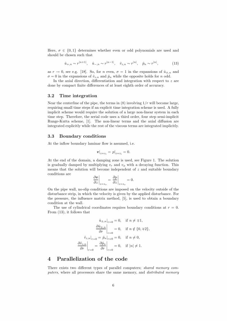
Here, σ ∈ 0, 1 determines whether even or odd polynomials are used andshould be chosen such that
u+,n ∼ r|n+1|, u−,n ∼ r|n−1|, vz,n ∼ r|n|, pn ∼ r|n|, (13)
as r → 0, see e.g. [18]. So, for n even, σ = 1 in the expansions of u±,n andσ = 0 in the expansions of vz,n and pn while the opposite holds for n odd.
In the axial direction, differentiation and integration with respect to z aredone by compact finite differences of at least eighth order of accuracy.
3.2 Time integration
Near the centerline of the pipe, the terms in (8) involving 1/r will become large,requiring small time steps if an explicit time integration scheme is used. A fullyimplicit scheme would require the solution of a large non-linear system in eachtime step. Therefore, the serial code uses a third order, four step semi-implicitRunge-Kutta scheme, [1]. The non-linear terms and the axial diffusion areintegrated explicitly while the rest of the viscous terms are integrated implicitly.
3.3 Boundary conditions
At the inflow boundary laminar flow is assumed, i.e.
v|z=zi= p|z=zi
= 0.
At the end of the domain, a damping zone is used, see Figure 1. The solutionis gradually damped by multiplying vr and vφ with a decaying function. Thismeans that the solution will become independent of z and suitable boundaryconditions are
∂v
∂z
∣
∣
∣
∣
z=zo
=∂p
∂z
∣
∣
∣
∣
z=zo
= 0.
On the pipe wall, no-slip conditions are imposed on the velocity outside of thedisturbance strip, in which the velocity is given by the applied disturbance. Forthe pressure, the influence matrix method, [5], is used to obtain a boundarycondition at the wall.
The use of cylindrical coordinates requires boundary conditions at r = 0.From (13), it follows that
u±,n|r=0= 0, if n 6= ∓1,
∂u±,n
∂r
∣
∣
∣
∣
r=0
= 0, if n /∈ 0,∓2,
vz,n|r=0= pn|r=0
= 0, if n 6= 0,
∂vz,n
∂r
∣
∣
∣
∣
r=0
=∂pn
∂r
∣
∣
∣
∣
r=0
= 0, if |n| 6= 1.
4 Parallelization of the code
There exists two different types of parallel computers; shared memory com-
puters, where all processors share the same memory, and distributed memory
6

computers, where the processors have their own memory which is not accessibleto other processors. Parallelizing a serial code is usually more straight forwardfor shared memory computers. In this case, the process of parallelizing typicallyamounts to inserting instructions, using e.g. OpenMP, at the places in the serialcode where tasks can be run in parallel. No sending of data between the pro-cessors is necessary, since they all have access to the same memory. However,shared memory computers in general have poor scalability; adding additionalprocessors slows down memory access time for all processors. Therefore, sharedmemory systems are usually not larger than 10−100 processors, although largersystems exist. Distributed memory computers do not suffer from this problem,since each processor has its own memory bus. However, when data in one pro-cessor is needed in another processor, the data must explicitly be sent, using e.g.MPI instructions, through the high-speed network connecting the processors.This adds a level of complexity to the parallelization.
The superior scalability of distributed memory computers makes them at-tractive despite the increase in parallelization complexity. Indeed, most existingparallel systems are of distributed type. At the Royal Institute of Technology,there is a distributed memory computer with approximately 600 processors openfor general use. We therefore chose to parallelize the code for distributed mem-ory computers.
4.1 Parallelization for a distributed memory computer
When parallelizing a serial code for a distributed memory computer, the workand data must be divided among the processors. The complexity of this varydrastically depending on the problem at hand; it varies from embarrassingly
parallel problems, which are such that they can easily be divided into many smallindependent problems, to inherently serial problems, for which parallelizationis virtually futile.
As an example of a problem which can easily be divided into smaller problemsthat are almost independent, consider differentiation of a function. Assume wewant to compute the derivative of f(x) on a uniform grid, xi, i = 0..N + 1,using central finite differences. We then want to evaluate
f ′(xi) ≈ (f(xi+1) − f(xi−1))/(2∆x), i = 1..N,
where ∆x is the distance between two grid points. For simplicity, let N be evenand let two processors be used for the differentiation. Partition the grid intotwo parts of equal size, i.e. processor one has the grid xi, i = 0..N/2 andprocessor two has the grid xi, i = N/2 + 1..N + 1. Now, both processors canindependently of each other compute the derivative in all their points exceptat the points closest to where the grid is divided, see Figure 2. In order tocompute f ′(xN/2), processor one needs the value of f(xN/2+1) which is locatedin processor two. Similarly, processor two needs the value of f(xN/2) fromprocessor one in order to compute f ′(xN/2+1). By explicitly using sending andreceiving routines, these values are sent between the processors and the finalderivatives are computed. The extension to more than two processors is straightforward. As long as the grid is large enough, such that each processor containsa fair amount of grid points, the time it takes to send data between processorswill be negligible compared to the time spent on computations.
7

Processor 1 Processor 2
xi xj
f ′(xi) f ′(xj)
xN2
xN2
+1
f ′(xN2
) f ′(xN2
+1)
Figure 2: Computing f ′(x) on two processors. The values of f(x) at xN2
and
xN2
+1 are sent between the processors.
4.2 Parallelization of the pipe Poiseuille code
In the serial code described in the previous section, there is no obvious way todivide the work among processors. For example, differentiation with respect tor is done by recursion relations for the Chebyshev coefficients. If fl, l = 0..L arethe Chebyshev coefficients of the function f(r), then the coefficients of g(r) =∂f/∂r are given by
gl−1 − gl+1 = 2lfl, l ≥ 1, (14)
with gL = 0 and gL−1 = 2LfL. Parallelizing (14) for two processors is easy, sincethe even and odd coefficients of g(r) are independent of each other. However,using more than two processors severely increases the parallelization complex-ity. Computing (14) amounts to solving a banded linear system. The straightforward approach of backward and forward substitution is inherently serial. Al-though there are (direct) methods for solving banded systems in parallel, [24],they generally show poor performance. The same problem is present in theaxial direction. Integration and differentiation with respect to z is done bycompact finite differences which also requires solving banded linear systems. Inthe azimuthal direction, the convolution sums (11) are not easily computed inparallel.
In order to overcome these problems, we chose to divide the domain in boththe axial and the azimuthal directions. Note that if the non-linear terms, ζ·,·,in (8) and (9) were somehow known, the problem of solving (8–10) is embar-rassingly parallel. All wave numbers, n, would then be independent of eachother and we could distribute an equal amount of wave numbers on each pro-cessor. Clearly, the non-linear terms are not known but must be computed from(11). As mentioned above, this is not a trivial task if different wave numbersare located on different processors. However, if the domain is divided only inthe axial direction, evaluating (11) is straight forward with the exception of theterms with derivatives with respect to z.
Our partitioning strategy thus involves dividing the domain in two directionsbut not in both directions simultaneously. The partitioning of data changesbetween being divided in the azimuthal direction and the axial direction asneeded. In practice, we do this by storing duplicate solutions. One solution ispartitioned in the axial direction so that each processor gets approximately thesame number of grid points. The other solution is partitioned in the azimuthaldirection such that each processor gets the same number of wave numbers. When
8
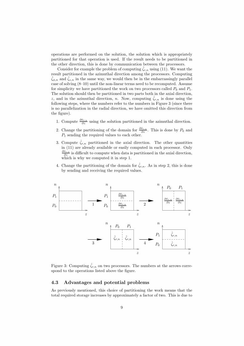
operations are performed on the solution, the solution which is appropriatelypartitioned for that operation is used. If the result needs to be partitioned inthe other direction, this is done by communication between the processors.
Consider for example the problem of computing ζr,n using (11). We want theresult partitioned in the azimuthal direction among the processors. Computingζφ,n and ζz,n in the same way, we would then be in the embarrassingly parallelcase of solving (8–10) until the non-linear terms need to be recomputed. Assumefor simplicity we have partitioned the work on two processors called P0 and P1.The solution should then be partitioned in two parts both in the axial direction,z, and in the azimuthal direction, n. Now, computing ζr,n is done using thefollowing steps, where the numbers refer to the numbers in Figure 3 (since thereis no parallelization in the radial direction, we have omitted this direction fromthe figure).
1. Compute∂vr,n
∂z using the solution partitioned in the azimuthal direction.
2. Change the partitioning of the domain for∂vr,n
∂z . This is done by P0 andP1 sending the required values to each other.
3. Compute ζr,n partitioned in the axial direction. The other quantitiesin (11) are already available or easily computed in each processor. Only∂vr,n
∂z is difficult to compute when data is partitioned in the axial direction,which is why we computed it in step 1.
4. Change the partitioning of the domain for ζr,n. As in step 2, this is doneby sending and receiving the required values.
P0
P0
P0
P0P0
P1
P1
P1
P1P1
n
n
n
nn
z
z
z
zz
1 ∂vr,n
∂z
∂vr,n
∂z ∂vr,n
∂z∂vr,n
∂z2
3 4 ζr,n
ζr,nζr,nζr,n
Figure 3: Computing ζr,n on two processors. The numbers at the arrows corre-spond to the operations listed above the figure.
4.3 Advantages and potential problems
As previously mentioned, this choice of partitioning the work means that thetotal required storage increases by approximately a factor of two. This is due to
9

the duplicate storing of the solution. This is a minor problem since typically, aserial code is not parallelized for using two processors only. A potentially moresevere problem is the large amounts of communication needed. Advancing thesolution one time step requires sending the entire solution (or therefrom derivedquantities) between the processors several times. This could be devastating tothe performance of the parallel code. As we will see in the next section, ourtests show that the time spent on communication is still small compared tothe computational time. This is due to the fast communication network on thecomputer used.
Also, performance is not the only issue when deciding on how to divide thework among processors. If we instead had chosen to partition the data onlyin the axial direction, the required communication would have reduced signif-icantly. However, we would then have been forced to solve the banded linearsystems from the compact finite differences in parallel. As mentioned above,direct parallel solvers for banded systems are typically inefficient. Instead, iter-ative solvers are usually preferred in parallel. Although this could have resultedin an efficient code as well, the amount of changes to the serial code would havebeen significantly larger.
5 Performance of the parallel code
In order to investigate the efficiency of the parallel code, we solved two problemsusing different number of processors. For both problems, we computed thespeedup, SP , and efficiency, EP , defined as
SP =TS
TP,
EP =SP
P,
where TS is the execution time for the serial code and TP is the execution timefor the parallel code using P processors. Ideally, the speedup should be linear,i.e. SP = P , which gives the optimal efficiency EP = 1.
Even if linear speedup is achieved for small P , it will eventually deteriorateas P increases. Obviously, this occurs when P is larger than the total amountof work available, leading to the fact that some processors remain idle duringthe entire execution. In reality, linear speedup typically deteriorates long be-fore this point since the communication time and increased overhead becomesincreasingly significant with increasing number of processors.
It is even possible to achieve better than linear speedup, so called super linearspeedup. This is due to memory effects. A computer has a hierarchical structureof different memory types. The fastest and smallest (∼ 1 MB) memory is thecache memory (actually, there are two or even three different cache memorieson a computer). Obviously, a typical application on a computer is too largeto be stored in the cache memory alone. Instead, most parts are stored in theRAM memory, which is larger (∼ 1 GB) but also several times slower than thecache memory. When an application is too large for the RAM memory, diskstorage is used. Disk storage is large (∼ 100 GB or more) but also orders ofmagnitude slower than the RAM memory. Super linear speedup can easily beachieved when a problem is so large that disk storage must be used in the serial
10

case. By dividing the problem on several processors, each processor can use onlythe RAM memory for its local part of the problem. The orders of magnitudein reduced memory access time easily makes up for the extra work required forsolving the problem in parallel. Even when disk storage is not required, theincrease in total cache memory when using several processors can give superlinear speedup. We will see an example of this in the second test problem inthe next section.
For both problems, we used the Dell Xeon cluster Lenngren at the Center forParallel Computers at the Royal Institute of Technology, Stockholm, Sweden.Lenngren consists of 442 nodes (although approximately 300 nodes are open forgeneral use), each having two 3.4 GHz ”Nocona” Xeon processors and 8 GB ofmain memory. MPI communication uses an Infiniband network from Mellanoxwith a bi-directional peak bandwidth of 2 GB/s.
Since the computer has two processors per node, they will share the com-munication and memory bandwidth when both are used. Hence, using onlyone processor per node gives faster communication and memory access. Wesolved the problems using one as well as both processors on each node. Thedifference in speedup between the two cases illustrate the importance of fastcommunication and memory access.
5.1 The first test problem
First, we consider a relatively small problem with 150 points in the axial direc-tion, 40 Fourier modes in the azimuthal direction and 20 Chebyshev polynomialsin the radial direction, giving a total of 1.2·105 degrees of freedom. The speedupand efficiency for this problem are shown in Figures 4 and 5.
0 2 4 6 8 10 12 14 16 18 200
2
4
6
8
10
12
14
16
18
20
P
SP
Figure 4: Speedup, SP , for the first test problem. The (*) are the results usingone processor per node and the () are the results using two processors pernode. The dashed line corresponds to linear speedup.
When using only one processor per node, an efficiency above 0.75 is achievedup to 10 processors. The large difference in speedup when one or both processorson the nodes are used clearly shows the need of fast communication and memoryaccess. When 20 processors are used, the speedup is rather poor. This is notsurprising, since the problem is quite small.
11

0 2 4 6 8 10 12 14 16 18 20
0.4
0.5
0.6
0.7
0.8
0.9
1
P
EP
Figure 5: Efficiency, EP , for the first test problem. The (*) are the resultsusing one processor per node and the () are the results using two processorsper node.
5.2 The second test problem
In the second test, we use 600 , 150 and 150 degrees of freedom in the axial, az-imuthal and radial directions, respectively, giving a total of 1.35 ·107 unknowns.The problem size is chosen such that the serial code uses most of the availableRAM memory. Therefore, the problem can not be solved in parallel on a singlenode using two processors, since the parallel code requires approximately twiceas much memory. The measured speedup and efficiency are shown in Figures 6and 7.
0 5 10 15 20 250
5
10
15
20
25
P
SP
Figure 6: Speedup, SP , for the second test problem. The (*) are the resultsusing one processor per node and the () are the results using two processorsper node. The dashed line corresponds to linear speedup.
We observe good speedup up to 15 processors; when using one processor pernode, the speedup is even super linear. This is due to memory effects discussedpreviously in this section. As in the first test problem, the speedup changessignificantly when one or both processors per node are used.
12
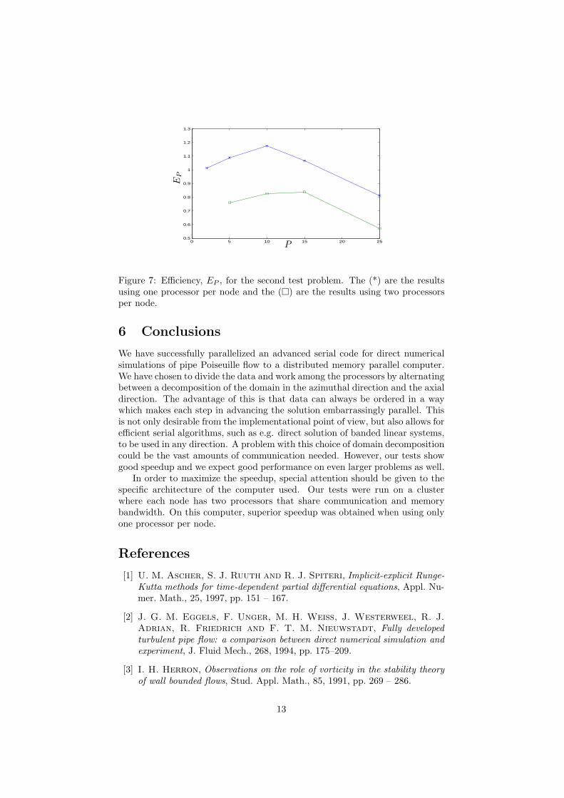
0 5 10 15 20 250.5
0.6
0.7
0.8
0.9
1
1.1
1.2
1.3
P
EP
Figure 7: Efficiency, EP , for the second test problem. The (*) are the resultsusing one processor per node and the () are the results using two processorsper node.
6 Conclusions
We have successfully parallelized an advanced serial code for direct numericalsimulations of pipe Poiseuille flow to a distributed memory parallel computer.We have chosen to divide the data and work among the processors by alternatingbetween a decomposition of the domain in the azimuthal direction and the axialdirection. The advantage of this is that data can always be ordered in a waywhich makes each step in advancing the solution embarrassingly parallel. Thisis not only desirable from the implementational point of view, but also allows forefficient serial algorithms, such as e.g. direct solution of banded linear systems,to be used in any direction. A problem with this choice of domain decompositioncould be the vast amounts of communication needed. However, our tests showgood speedup and we expect good performance on even larger problems as well.
In order to maximize the speedup, special attention should be given to thespecific architecture of the computer used. Our tests were run on a clusterwhere each node has two processors that share communication and memorybandwidth. On this computer, superior speedup was obtained when using onlyone processor per node.
References
[1] U. M. Ascher, S. J. Ruuth and R. J. Spiteri, Implicit-explicit Runge-
Kutta methods for time-dependent partial differential equations, Appl. Nu-mer. Math., 25, 1997, pp. 151 – 167.
[2] J. G. M. Eggels, F. Unger, M. H. Weiss, J. Westerweel, R. J.
Adrian, R. Friedrich and F. T. M. Nieuwstadt, Fully developed
turbulent pipe flow: a comparison between direct numerical simulation and
experiment, J. Fluid Mech., 268, 1994, pp. 175–209.
[3] I. H. Herron, Observations on the role of vorticity in the stability theory
of wall bounded flows, Stud. Appl. Math., 85, 1991, pp. 269 – 286.
13
[4] B. Hof, A. Juel and T. Mullin, Scaling of the turbulence transition
threshold in a pipe, Phys. Rev. Lett., 91(24), 2003, 244502.
[5] L. Kleiser and U. Schumann, Treatment of incompressibility and bound-
ary conditions in 3-D numerical simulations of plane channel flows, Proc.third GAMM.-conference on numerical methods in fluid mechanics, 1980,pp. 165–173.
[6] G. Kreiss, A. Lundbladh and D. S. Henningson, Bounds for threshold
amplitudes in subcritical shear flows, J. Fluid Mech., 270, 1994, pp. 175–198.
[7] M. Lessen, S. G. Sadler and T.-Y. Liu, Stability of pipe Poiseuille
flow, Phys. Fluids, 11, 1968, pp. 1404–1409.
[8] P. Loulou, R. D. Moser, N. N. Mansour and B. J. Cantwell,Direct numerical simulation of incompressible pipe flow using a b-spline
spectral method, Technical Memorandum TM-110436, NASA, 1997.
[9] A. Lundbladh, D. S. Henningson and S. C. Reddy, Threshold am-
plitudes for transition in channel flows, Transition ,Turbulence, and Com-bustion, M. Y. Hussaini, T. B. Gatski, and T. L. Jackson, eds., Vol. I,Kluwer, Dordrecht, Holland, 1994, pp. 309–318.
[10] B. Ma, C. W. H. Van Doorne, Z. Zhang and F. T. M. Nieuw-
stadt, On the spatial evolution of a wall-imposed periodic disturbance in
pipe Poiseuille flow at Re = 3000. Part 1. Subcritical disturbance, J. FluidMech., 398, 1999, pp. 181 – 224.
[11] F. Mellibovsky and A. Meseguer, The role of streamwise perturbations
in pipe flow transition, Phys. Fluids, 18, 2006, 074104.
[12] A. Meseguer and F. Mellibovsky, On a solenoidal Fourier-Chebyshev
spectral method for stability analysis of the Hagen-Poiseuille flow, Appl.Numer. Math. (2006), doi:10.1016/j.apnum.2006.09.002.
[13] A. Meseguer and L. N. Trefethen, Linearized pipe flow to Reynolds
number 107, J. Comput. Phys., 186, 2003, pp. 178–197.
[14] T. Mullin and J. Peixinho, Transition to turbulence in pipe flow, J.Low Temp. Phys., 145, 2006, pp. 75–87.
[15] N. V. Nikitin, Statistical characteristics of wall turbulence, Fluid Dyn.,31, 1996, pp. 361–370.
[16] S. A. Orszag and A. T. Patera, Secondary instability off wall-bounded
shear flows, J. Fluid Mech., 128, 1983, pp. 347–385.
[17] P. L. O’Sullivan and K. S. Breuer, Transient growth in circular pipe
flow. I. Linear disturbances, Phys. Fluids, 6, 1994, pp. 3643–3651.
[18] V. G. Priymak and T. Miyazaki, Accurate Navier-Stokes investigation
of transitional and turbulent flows in a circular pipe, J. Comput. Phys.,142, 1998, pp. 370–411.
14

[19] S. C. Reddy, P. J. Schmid, J. S. Bagget and D. S. Henningson,On stability of streamwise streaks and transition thresholds in plane channel
flows, J. Fluid Mech., 365, 1998, pp. 269 – 303.
[20] J. Reuter and D. Rempfer, Analysis of pipe flow transition. Part I.
Direct numerical simulation, Theoret. Comput. Fluid Dynamics, 17, 2004,pp. 273 – 292.
[21] P. J. Schmid and D. S. Henningson, Optimal energy density growth in
Hagen-Poiseuille flow, J. Fluid Mech., 277, 1994, pp. 197–225.
[22] H. Shan, B. Ma, Z. Zhang and F. T. M. Nieuwstadt, Direct numer-
ical simulation of a puff and a slug in transitional cylindrical pipe flow, J.Fluid Mech., 387, 1999, pp. 39–60.
[23] L. N. Trefethen, A. E. Trefethen, S. C. Reddy and T. A.
Driscoll, Hydrodynamic stability without eigenvalues, Science, 261, 1993,pp. 578 – 584.
[24] E. F. Van de Velde, Concurrent scientific computing, Springer, 1994.
[25] R. Verzicco and P. Orlandi, A finite-difference scheme for three-
dimensional incompressible flows in cylindrical coordinates, J. Comput.Phys., 123, 1996, pp. 402–414.
[26] O. Y. Zikanov, On the instability of pipe Poiseuille flow, Phys. Fluids, 8,1996, pp. 2923–2932.
[27] P.-O. Asen and G. Kreiss, Resolvent bounds for pipe Poiseuille flow, J.Fluid Mech., 568, 2006, pp. 451 – 471.
15

Theoretical and Computational Fluid Dynamics manuscript No.(will be inserted by the editor)
Per-Olov Asen · Gunilla Kreiss · Dietmar Rempfer
Direct numerical simulations of localized disturbances inpipe Poiseuille flow
Received: date / Accepted: date
Abstract We consider pipe Poiseuille flow subjected to a disturbance which is highly localized in space.Experiments by Mullin and Peixinho have shown this disturbance to be efficient in triggering turbulence,yielding a threshold dependence on the required amplitude as R−1.5 on the Reynolds number,R. The experi-ments also indicate an initial formation of hairpin vortices, with each hairpin having a length of approximatelyone pipe radius, independent of the Reynolds number in the range ofR = 2000 to 3000. We perform directnumerical simulations forR = 5000. The results show a packet of hairpin vortices traveling downstream, eachhaving a length of approximately one pipe radius. The perturbation remains highly localized in space whilebeing advected downstream for approximately 10 pipe diameters. Beyond that distance from the disturbanceorigin the flow becomes severely disordered.
Keywords direct numerical simulations, pipe Poiseuille flow, hydrodynamical stability, incompressibleNavier–Stokes equations
PACS 47.11.-j· 47.20.Ft· 47.27.ek
1 Introduction
Hydrodynamical stability concerns the stability of various flows when subjected to disturbances. A givenstationary flow is called stable if the perturbation generated by a disturbance eventually vanishes, i. e. if theflow returns to the stationary state. If the flow is not stable to a disturbance, it may eventually develop into aturbulent state. Despite a long history of research in the area, the onset of turbulence is not well understood.Controlling the presence of turbulence would be of significant importance in many real-world applications. Abetter understanding of the onset of turbulence is crucial for achieving this.
Pipe Poiseuille flow was first studied experimentally by Osborne Reynolds at the end of the 19th century.He found that the sensitivity to disturbances could be characterized by one non-dimensional number, theReynolds number,R. For Reynolds numbers smaller than about 2000, the flow was observed to be stable to alldisturbances. He also found that laminar flow could be maintained at higher Reynolds numbers by avoidingdisturbing the flow; increasing Reynolds number required increasing care in avoiding disturbances. In theexperiments, laminar flow was observed up to Reynolds numbers around 12000. The findings of Reynolds
P.-O.AsenLinne Flow Centre, CSC, KTH, Lindstedtsv. 3, SE-100 44 Stockholm, Sweden.Tel.: +46-8-790 69 27Fax: +46-8-790 64 57E-mail: [email protected]
G. KreissDepartment of Information Technology, Uppsala University, Box 120, S-751 04 Uppsala, Sweden.
D. RempferIllinois Institute of Technology, 243c Engineering1, 3110South State Street, Chicago, IL 60616, USA.

2 Per-OlovAsen et al.
have since then been verified in numerous experiments. A critical Reynolds number, below which the flow isstable to all disturbances, aroundRc ≈ 1800 has been found [24] and in highly controlled experiments laminarflow has been maintained up toR = 105 [25].
From a mathematical point of view, the most straightforwardway to investigate the stability propertiesof a stationary flow is to consider the linearized Navier–Stokes equations. If the linear operator associatedwith these equations has, at some Reynolds number, an eigenvalue with positive real part, then the flow islinearly unstable. This would imply that there exist infinitesimal disturbances that will make the flow unstable.However, numerous numerical computations have been done without finding any unstable eigenvalues for pipePoiseuille flow, see e. g. [13,19,29]. Also, rigorous results have been proven that show that pipe Poiseuilleflow is linearly stable, at any Reynolds number, to axisymmetric disturbances [8] as well as to certain non-axisymmetric disturbances [3]. Despite the believed linear stability of pipe Poiseuille flow, disturbances mayexhibit severe initial growth due to linear effects. This iscommonly referred to astransient growth, and is dueto the non-normality of the operator of the linearized Navier–Stokes equations [31].
To understand transition to turbulence, nonlinear effectsmust also be taken into account; assuming theflow is linearly stable, it is clear that nonlinear effects are necessary at some point in the transition to turbu-lence. The question ofnonlinear stability of pipe Poiseuille flow has long been a main point ofinterest. Ithas been suggested that linearly stable shear flows are stable to all disturbances with amplitudes smaller thansome threshold value, which scales with the Reynolds numberasR−β for someβ ≥ 1 [31]. Determining thecorrect value ofβ for pipe Poiseuille flow has proven to be a difficult task. Which mechanisms are dominantin the evolution of a perturbation is also far from understood. Further knowledge in this would not only assistin determiningβ , but also provide insight in the process of transition from laminar flow to turbulence.
In the last decades, computers have become powerful enough to simulate flows in simple geometriesusing direct numerical simulations (DNS). DNS means that the full nonlinear Navier–Stokes equations aresolved numerically such that all length-scales are resolved. This requires numerical methods of high orderof accuracy as well as vast amounts of computer resources. The precise control of the disturbance and thepossibility to analyze the evolution of the resulting perturbation in detail makes DNS an excellent tool ininvestigating transition to turbulence. For example, bothfor plane Couette flow and plane Poiseuille flow,DNS has been used to determine upper bounds onβ and also to investigate different transition scenarios,see e. g. [12,15,27]. Also, a critical Reynolds number around Rc ≈ 1800 in pipe flow has been verified usingDNS [34].
For pipe Poiseuille flow, experiments in e. g. [9,20] indicate β ≈ 1. In [9], the flow was disturbed byinjection of fluid through six equally spaced small holes around the pipe while in [20], injection through asingle hole was used. In more recent (not yet published) experiments, Mullin and Peixinho disturbed the flowby a combination of injection and suction through two holes located close to each other. The experimentsshowed that the required amplitude for triggering turbulence using this disturbance is an order of magnitudesmaller than when disturbing with injection in a single hole. Moreover, the experiments showed that thelocation of the holes relative to each other have significanteffect; when the holes are either aligned with orperpendicular to the pipe axis, the resulting threshold exponent isβ ≈ 1.3, while locating the holes such thatthey form a 45-degree angle with the pipe axis results inβ ≈ 1.5. Clearly, the stability of pipe flow is highlydependent on the disturbance used.
So far, only a handful of codes for DNS of pipe Poiseuille flow have been developed. This is mainlydue to the additional complexity of solving the equations incylindrical coordinates, as opposed to channelflow, where Cartesian coordinates are used. Some of the existing codes are based on methods of low order ofaccuracy in one or more spatial directions, e. g. [6,21,33,35]. Also, most codes with high order of accuracyare, to the authors knowledge, written for serial computers, e. g. [14,18,23], although parallel, high ordercodes exist (see [16], which is based on the serial code presented in [30]).
Simulations have previously been used in order to determinea value ofβ for pipe Poiseuille flow; ex-tensive computations in [17] suggestβ = 1.5. However, the disturbance considered in [17] correspondsto aninitial condition of streamwise independent structures which are chosen to optimally trigger instability. Ex-perimental investigation of such structures is difficult, since disturbances in experiments are typically appliedusing relatively high velocity injection or suction in small holes in the pipe wall. Such large and spatially lo-calized disturbances add additional requirements on the resolution of a simulation mimicking the experiments.This makes the use of a serial code insufficient.
In this paper, we demonstrate the possibility of using direct numerical simulations for disturbances withhigh spatial locality, making comparisons with experiments possible as well as providing detailed insight intothe early development of the perturbations. In particular,we present results from a simulation atR = 5000
Direct numerical simulations of localized disturbances inpipe Poiseuille flow 3
where the perturbation is triggered by a disturbance similar to the most efficient disturbance used in theexperiments of Mullin and Peixinho, i. e. when the holes makea 45-degree angle with the pipe axis. Thesimulation was done using a parallelized version of a serialcode developed by Reuter and Rempfer [28],based on compact finite differences of at least eighth order of accuracy in the axial direction and Fourier andChebyshev expansions in the azimuthal and radial directions, respectively.
The paper is organized as follows: In section 2, we present the mathematical formulation of the problem.Section 3 summarizes the numerical methods in the serial code developed by Reuter and Rempfer [28], andalso the parallelization of the code [2]. In section 4, we describe the experiments by Mullin and Peixinho andhow the experiments are modeled in the simulations. The results of the simulations are presented in section 5,followed by our conclusions in section 6.
2 Mathematical background
We consider the flow of an incompressible fluid in an infinite circular pipe where the flow is driven by aconstant pressure gradient in the axial direction. The governing equations are the Navier-Stokes equations.Let the vectorU denote the velocity field in the pipe and let the scalar valuedfunctionP denote the pressurerelative to a reference pressure. Then, the equations describing the evolution ofU andP are
∂U
∂ t+U · ∇ U =
4R
ez − ∇ P+1R
∆U , (1)
∇ ·U = 0, (2)
whereez is the unit vector in the axial direction. On the boundary, weenforce no-slip conditions, i. e.U = 0on the pipe wall.
Equations (1) and (2) have been non-dimensionalized using the Reynolds number,R, which in this case isdefined as
R =2Uza
ν, (3)
whereUz is the mean velocity in the axial direction,a is the pipe radius andν is the kinematic viscosity ofthe fluid. Note that the quantities on the right hand side of (3) are dimensional quantities whileU andP in (1)and (2) are non-dimensional.
If equations (1) and (2) are written in cylindrical coordinates, a stationary solution,(V ,Ps), in the domainΩ = (r,φ,z)|0≤ r ≤ 1,0≤ φ ≤ 2π,z ∈ R is given by
V (r) = (Vr,Vφ,Vz) = Vrer +Vφeφ +Vzez = (1− r2)ez,
Ps(z) = −4R
z+P0,
whereP0 is a constant ander, eφ andez are the unit-vectors in the radial, azimuthal and axial directions,respectively.
Let v(t,r,φ,z) = (vr,vφ,vz) and p(t,r,φ,z) denote the perturbation of the stationary solution. By substi-tutingU = V +v andP = Ps + p into (1) and (2), corresponding equations for the perturbation are obtained.However, in cylindrical coordinates, the Laplacian is not diagonal, i. e.er ·∆v andeφ ·∆v both involvevr andvφ. Using a well-known reformulation, see e. g. [22],
u± = vr ± ivφ,
the Laplacian is diagonalized. The resulting two equationsfor u± are
∂u±∂ t
+ vr∂u±∂ r
+vφ
r
(
∂u±∂φ
± iu±
)
+(Vz + vz)∂u±∂ z
= −∂ p∂ r
∓ir
∂ p∂φ
+1R
[
1r
∂∂ r
(
r∂u±∂ r
)
+1r2
(
∂ 2u±∂φ2 ±2i
∂u±∂φ
−u±
)
+∂ 2u±∂ z2
]
.
(4)
The axial velocity,vz, can be obtained from (2), which in cylindrical coordinatesis given by
1r
∂ rvr
∂ r+
1r
∂vφ
∂φ+
∂vz
∂ z= 0. (5)

4 Per-OlovAsen et al.
An equation for the pressure is obtained by applying the divergence operator to (1) and using (2) to simplifythe obtained equation. The resulting Poisson equation is
1r
∂∂ r
(
r∂ p∂ r
)
−1r2
∂ 2p∂φ2 +
∂ 2p∂ z2 = −
1r
∂ rζr
∂ r−
1r
∂ζφ
∂φ−
∂ζz
∂ z, (6)
where
ζr = vr∂vr
∂ r+
vφ
r
(
∂vr
∂φ− vφ
)
+(Vz + vz)∂vr
∂ z,
ζφ = vr∂vφ
∂ r+
vφ
r
(
∂vφ
∂φ+ vr
)
+(Vz + vz)∂vφ
∂ z,
ζz = vr∂ (Vz + vz)
∂ r+
vφ
r∂vz
∂φ+(Vz + vz)
∂vz
∂ z.
The no-slip conditions on the pipe wall impliesv(t,1,φ,z) = 0.
3 Numerical methods
The code used in this paper is based on a serial code developedby Reuter and Rempfer which we paral-lelized for a distributed memory computer. For details of the serial code, we refer to [28], and in [2], detailsconcerning the parallelization can be found. This section is a brief summary of these two papers.
Equations (4–6) are solved in the domainD = (r,φ,z)|0 ≤ r ≤ 1,0 ≤ φ ≤ 2π,zi ≤ z ≤ zo for givenzi andzo, see Figure 1. A disturbance is introduced by applying non-homogeneous boundary conditions inone or more disturbance slots as shown in the figure. The serial code was verified by Reuter and Rempfer by
Inflow Outflow
Disturbance slot Damping zone
Fig. 1 Computational domain.
comparing with results from linear theory as well as experimental data.
3.1 Discretization
Let w ∈ vr,vφ,vz, p denote any of the components of the solution. In the azimuthal direction, the solution isapproximated by a finite Fourier series as
w(t,r,φ,z) =N
∑n=−N
wn(t,r,z)einφ. (7)
Since the sums must be real, they can be restricted ton ≥ 0.

Direct numerical simulations of localized disturbances inpipe Poiseuille flow 5
Inserting (7) in (4–6) yields
∂ u±,n
∂ t+ ζ±,n = −
∂ pn
∂ r±
npn
r+
1R
[
1r
∂∂ r
(
r∂ u±,n
∂ r
)
−(1±n)2u±,n
r2 +∂ 2u±,n
∂ z2
]
, (8)
1r
∂∂ r
(
r∂ pn
∂ r
)
−n2 pn
r2 +∂ 2pn
∂ z2 = −1r
∂ rζr,n
∂ r−
inζφ,n
r−
∂ ζz,n
∂ z, (9)
1r
∂ rvr,n
∂ r+
invφ,n
r+
∂ vz,n
∂ z= 0, (10)
for n = 0,1, ...N, where the nonlinear terms are given byζ±,n = ζr,n ± iζφ,n and
ζr,n = ∑n′ +n′′ = n|n′|, |n′′ | ≤ N
(
vr,n′∂ vr,n′′
∂ r+ vφ,n′
in′′vr,n′′ − vφ,n′′
r+ v+
z,n′∂ vr,n′′
∂ z
)
,
ζφ,n = ∑n′ +n′′ = n|n′|, |n′′ | ≤ N
(
vr,n′∂ vφ,n′′
∂ r+ vφ,n′
vr,n′′ + in′′vφ,n′′
r+ v+
z,n′∂ vφ,n′′
∂ z
)
,
ζz,n = ∑n′ +n′′ = n|n′|, |n′′ | ≤ N
(
vr,n′∂ v+
z,n′′
∂ r+ vφ,n′
in′′vz,n′′
r+ v+
z,n′∂ vz,n′′
∂ z
)
.
(11)
Here,
v+z,n =
Vz + vz,0 if n = 0,vz,n if n 6= 0.
Note that the nonlinear terms (11) result in interactions between different Fourier modes, e. g. modesn′ = 1andn′′ = 2 act as a forcing for then′+n′′ = 3 mode. This interaction is disregarded for modes withn′+n′′ > N.Therefore, the number of Fourier coefficients used in the computations must be sufficiently large, such thatthis truncation of nonlinear interaction has negligible effect on the final result.
In the radial direction, the solution is expanded in a finite Chebyshev series. The Chebyshev polynomials,Tk(x) = cos(k arccos(x)) for −1≤ x ≤ 1, are even/odd functions fork even/odd. The parity relation observedin e. g. [22] is used in order to avoid clustering of points near the center of the pipe. This means that eachcomponent of the solution is expanded in even or odd Chebyshev polynomials as
wn(t,r,z) =L
∑l=0
c2l+σ wn,l(t,z)T2l+σ(r), c2l+σ =
12 if 2l +σ = 0,1 if 2l +σ > 0.
Here,σ ∈ 0,1 determines whether even or odd polynomials are used and should be chosen such that
u+,n ∼ r|n+1|, u−,n ∼ r|n−1|, vz,n ∼ r|n|, pn ∼ r|n|, (12)
asr → 0, see e. g. [26]. So, forn even, odd polynomials,σ = 1, are used in the expansions of ˆu±,n and evenpolynomials,σ = 0, are used in the expansions of ˆvz,n and pn. For oddn the situation is reversed.
In the axial direction, differentiation and integration with respect toz are done by compact finite differ-ences. An advantage of compact finite differences is that high order of accuracy can be obtained using narrowstencils. This simplifies the treatment of points near the boundary, where non-symmetric stencils must beused. All formulas used in the code are of eighth order of accuracy or higher.
3.2 Time integration
Near the centerline of the pipe, the terms in (8) involving 1/r will become large, thus requiring a small timestep if an explicit integration scheme is used. A fully implicit scheme would require the solution of a largenonlinear system in each time step. The serial code uses a third order, four step semi-implicit Runge-Kutta

6 Per-OlovAsen et al.
scheme [1]. The nonlinear terms and the axial diffusion are integrated explicitly while the rest of the viscousterms are integrated implicitly.
Note that since the axial diffusion is integrated explicitly, the CFL condition gives a necessary boundon R−1∆ t/∆ z2 for stability. Similarly, for the advective term,vr∆ t/∆ r must be bounded, where∆ r is thedistance between collocation points in the radial direction. As mentioned above, expanding in even or oddChebyshev polynomials avoids the undesired clustering of points near the center of the pipe. However, theclustering is still present, and desired in order to resolvethe boundary layers, near the wall of the pipe where∆ r = O(1/L2). If no-slip conditions are enforced on the pipe wall, and theflow is driven by e. g. a volumeforcing or a given initial state, this is a minor problem sincevr is small near the wall. However, driving the flowwith locally large inhomogeneous boundary conditions forvr, the admissible time step is severely restricted.This has been observed in our computations.
3.3 Boundary conditions
At the inflow boundary, laminar flow is assumed, i. e.
v|z=zi= p|z=zi
= 0.
At the end of the domain, a damping zone is used, see Figure 1. The solution is gradually damped by multiply-ing vr andvφ with a decaying function. Hence, the solution becomes independent ofz and suitable boundaryconditions are
∂v
∂ z
∣
∣
∣
∣
z=zo
=∂ p∂ z
∣
∣
∣
∣
z=zo
= 0.
On the pipe wall, no-slip conditions are imposed on the velocity outside of the disturbance strip, in whichinhomogeneous boundary conditions are used to model an applied disturbance. For the pressure, the influencematrix method [11], is used to obtain a boundary condition atthe wall.
The use of cylindrical coordinates requires boundary conditions atr = 0. From (12), it follows that
u±,n|r=0 = 0, if n 6= ∓1,
∂ u±,n
∂ r
∣
∣
∣
∣
r=0= 0, if n /∈ 0,∓2,
vz,n|r=0 = pn|r=0 = 0, if n 6= 0,
∂ vz,n
∂ r
∣
∣
∣
∣
r=0=
∂ pn
∂ r
∣
∣
∣
∣
r=0= 0, if |n| 6= 1.
3.4 Parallelization
The numerical methods used in the serial code are of high order of accuracy. However, they yield a globaldata dependency, i. e. the solution can not easily be dividedinto parts which are almost independent whenintegrating one time step. For example, differentiation with respect tor is done by recursion relations for theChebyshev coefficients. Iffl, l = 0..L are the Chebyshev coefficients of the functionf (r), then the coefficientsof g(r) = ∂ f /∂ r are given by
gl−1− gl+1 = 2l fl, l ≥ 1, (13)
with gL = 0 and ˜gL−1 = 2L fL. Parallelizing (13) for two processors is easy, since the even and odd coefficientsof g(r) are independent of each other. However, when using more thantwo processors the parallelizationcomplexity is severely increased. Computing (13) amounts to solving a banded linear system. Although thereare (direct) methods for solving banded systems in parallel[32], they generally show poor performance. Thesame problem is present in the axial direction. Integrationand differentiation with respect toz is done bycompact finite differences which also requires solving banded linear systems. In the azimuthal direction, theconvolution sums (11) are not easily computed in parallel.
In order to overcome these problems, we partition the domainin two directions but not in both directionssimultaneously. The partitioning of data switches betweena division of in the azimuthal direction and a divi-sion of the axial direction as needed. In practice, we make this possible by storing duplicate solutions. One

Direct numerical simulations of localized disturbances inpipe Poiseuille flow 7
solution is partitioned in the axial direction so that each processor gets approximately the same number ofgrid points. The other solution is partitioned in the azimuthal direction such that each processor gets the samenumber of wave numbers. When operations are performed on thesolution, the solution which is appropri-ately partitioned for that operation is used. For example, when differentiating with respect toz, the solutionpartitioned in the azimuthal direction is used. If the result needs to be partitioned in the other direction, this isdone by communication between the processors.
This partitioning strategy requires large amounts of communication. However, our tests have shown goodspeedup [2].
4 Background and modeling
As mentioned in the introduction, we are interested in doingnumerical simulations in order to obtain fur-ther understanding of experimental results. In this section, we describe the experimental setup and also themathematical model of the experiments.
4.1 Experimental setup
Experiments using either injection and/or suction to disturb the flow have previously yielded a threshold forstability which scales asR−1 with the Reynolds number [5,9,20]. However, as noted in [20], the requiredamplitude for triggering turbulence can vary significantlydepending on the disturbance used; when usingsuction in a single hole, the required amplitude for triggering turbulence was typically two orders of magnitudelarger than in the case of injection in a single hole. Clearly, the stability of pipe flow is highly dependent onthe disturbance used.
In more recent experiments, Mullin and Peixinho disturbed the flow by applying injection and suctionthrough two small holes located close to each other. The experiments showed that the location of the holesrelative to each other have significant importance on how efficient the disturbance is at triggering turbulence.So far, the most efficient way to trigger turbulence has been when the holes are located such that a linethrough the center of both holes makes a 45-degree angle withthe pipe centerline, see Figure 2; both possibledisturbances, i. e. injection applied in the hole further upstream or the hole further downstream with suctionapplied in the other hole, are equally efficient. The disturbance is applied in holes with diameterd = 0.05D,whereD is the diameter of the pipe. The amplitude of the disturbanceis defined as the injected volume flux,Φin j, normalized with the pipe flux,Φpipe, i.e. the amplitude isΦin j/Φpipe. With this definition of amplitude,note that although small amplitudes may be required for triggering turbulence, the maximal velocity mightstill be large since the disturbance holes are small.
These experiments yield a threshold which scales asR−1.5 with the Reynolds number. Why this distur-bance is so efficient in triggering turbulence is not known. Flow visualizations in the experiments indicate theformation of so-called “hairpin vortices” which are known to play a central role in the transition to turbulencein boundary layers [4]. Numerical simulations can give further insight in this matter.
d
D
45
Flow direction
Fig. 2 Location of the disturbance holes in the experiments by Mullin and Peixinho.

8 Per-OlovAsen et al.
4.2 Mathematical model
We consider a disturbance applied through holes that are lined up to form a 45-degree angle with the pipeaxis and with injection applied in the hole further upstream, i. e. injection and suction is applied in the leftand right hole in Figure 2, respectively. The disturbance ishighly localized in space, both in the axial andazimuthal directions. We model the injection and suction bysetting non-homogeneous boundary conditionsas
vr(φ,z)|r=1 = Ae((φ−φ0)/ε)2f (z), (14)
for each disturbance slot. The locality of each disturbanceslot in the axial direction is modeled by the functionf (z). In order to avoid numerical difficulties,f (z) must be sufficiently smooth. The function we used is
f [x(z)] =
(1− x2)6, |x| ≤ 1,0, |x| ≥ 1,
x =z− zs
δ.
Here,zs is the position of the center andδ is the effective width of the slot.The parametersA, φ0 andε are chosen in each disturbance slot to model the maximal velocity and az-
imuthal shape of the applied injection or suction. Since thediameter of the pipe in the computations isD = 2,εshould be chosen such that the effective width in the azimuthal direction of (14) is approximately 0.05D = 0.1.This is achieved withε ≈ 0.03. However, since Fourier expansion is used in the azimuthal direction, theboundary condition (14) must be applied on the Fourier coefficients, i. e. (14) must be expanded in a finiteFourier series. In order to obtain a good approximation of (14) with ε = 0.03 as a finite Fourier series, about100 Fourier coefficients are needed. As previously mentioned, the number of Fourier coefficients used in thecomputations must be sufficiently large, such that the truncation of the nonlinear interactions between highwave numbers has negligible effect. Hence, applying inhomogeneous boundary conditions on 100 coefficientswould require numerical computations using even more (say≈ 200) coefficients. Modeling such a small holewould also require high resolution in the other two spatial directions. In the axial direction,∆ z must be smallin order to resolvef (z). A disturbance with a given volume flux requires a high maximal velocity in a smallhole, which in turn requires high resolution in the radial direction. Making things even worse, the time stepmust be small due to the high spatial resolution and the high maximal velocity near the wall.
We therefore model the experimental disturbance withε = 0.1, which gives holes of a diameter of approx-imately 0.3, i. e. three times larger than the holes in the experiments.The locations in the azimuthal directionof the inhomogeneous boundary conditions areφ0 = π andφ0 = π+0.6 for the injection and suction, respec-tively and the maximal velocity of both isA = 0.5. We represent the inhomogeneous boundary conditionsusing 40 Fourier coefficients, which results in the functions seen in Figure 3. Note that although we use 40Fourier coefficients, the resulting functions are still somewhat oscillatory.
(a) (b)
0 1 2 3 4 5 6
−0.5
−0.4
−0.3
−0.2
−0.1
0
0.1
φ
v r| r
=1
0 1 2 3 4 5 6−0.1
0
0.1
0.2
0.3
0.4
0.5
φ
v r| r
=1
Fig. 3 Resulting boundary conditions for (a) injection atz = −0.3 and (b) suction atz = 0.3 using 40 Fourier coefficients.
Corresponding to a diameter of 0.3, we chooseδ = 0.3 and the centers of the injection and suction atzs = −0.3 andzs = 0.3, respectively. This results in the functionsf (z) shown in Figure 4.

Direct numerical simulations of localized disturbances inpipe Poiseuille flow 9
−0.6 −0.4 −0.2 0 0.2 0.4 0.60
0.1
0.2
0.3
0.4
0.5
0.6
0.7
0.8
0.9
1
z
f(z)
Fig. 4 The functionf (z) in the boundary condition (14). Solid is for the injection and dashed is for the suction.
5 Numerical results
In this section, we present results from a simulation using the inhomogeneous boundary conditions describedabove. The inhomogeneous boundary conditions were appliedat timet = 0 and “kept on” during the entiresimulation until the end time,t ≈ 75.4. In order to avoid large gradients in the initial stage, a gradual increasefrom no-slip conditions was used in the time spant ∈ [0,0.25]. In this simulation, the Reynolds number wasR = 5000 and the length of the pipe was 60= 30D.
Since the inhomogeneous boundary conditions are very localized is space, a high resolution is necessary.We used a grid withN = 100 Fourier modes,L = 200 Chebyshev polynomials and 1500 grid points (∆ z =0.04) in the axial direction. The time integration was done using the time step∆ t ≈ 0.0031, requiring a totalof 24000 time steps to reach the end time.
The simulation was run on the Dell Xeon cluster “Lenngren” atthe Center for Parallel Computers atthe Royal Institute of Technology, Stockholm, Sweden, consisting of 442 nodes, each having two 3.4 GHz”Nocona” Xeon processors and 8 GB of main memory. MPI communication uses an Infiniband network fromMellanox with a bi-directional peak bandwidth of 2 GB/s. We used 50 processors for our computation whichrequired a total of approximately 10300 CPU-hours or 1.17 CPU-years.
We study and present results at two different stages; the initial stage and the late stage. The initial stagedescribes the evolution for short times, when the perturbation velocity is still somewhat ordered and localizedin the radial direction, while the late stage concerns the transition to a more global and disordered perturbationvelocity field.
The main question addressed in this paper is the one of why theapplied injection and suction is so efficientin triggering turbulence. The initial stage is the most interesting from this point of view, since it is directlyconnected to the way the perturbation is generated. The later stage has little or no relation to the origin of theperturbation and should be analyzed using averaged quantities which is the subject of upcoming work. Still,we present some results here, mainly to demonstrate the capabilities of the parallel code but also to makeplausible that the computations are sufficiently resolved to simulate turbulent flow.
5.1 Initial stage
Immediately downstream of the disturbance slots, a pair of counter-rotating vortices are excited close to thewall, see Figure 5. The axial velocity of the laminar flow is higher close to the center of the pipe than near thewall. The vortices force high speed fluid towards the wall andlow speed fluid towards the center, generatingthe high- and low-speed streaks seen in Figure 5.
The structure of the vortices can be visualized by a method proposed in [10]. In short, the method is basedon studying iso-surfaces of the second eigenvalue,λ2, of S2 + Ω2, whereS andΩ are the symmetric andantisymmetric parts of the gradient of the velocity,∇ v.
In Figure 6, iso-surfaces ofλ2 = −0.5 are shown at two different times. Also shown are the high-speedstreaks located close to the pipe wall and the low-speed streaks located closer to the center of the pipe. As

10 Per-OlovAsen et al.
(a) (b)
Fig. 5: Perturbation velocity field at (a)z = 1 and (b)z = 5 whent ≈ 12.6. Red corresponds tovz = 0.3 andblue representsvz = −0.5. The spacing between the contour lines is 0.1 and the zero contour is dashed. Thearrows show the perturbation velocity in the plane.
seen in the figure, the perturbation evolves in the form of hairpin vortices. The hairpins appear in a ratherstructured fashion, with both individual length and distance between two hairpins of approximately one piperadius. This is in good agreement with the experiments of Mullin and Peixinho, where hairpins of length onepipe radius, independent of the Reynolds number over the range 2000 to 3000, were found.
The high- and low-speed streaks created by the hairpin vortices results in localized layers of high shear.The development of these high-shear layers are shown in Figure 7. The hairpins are created close to the wall,and as they are advected downstream, they move closer to the center of the pipe.
5.1.1 Numerical resolution
In order to investigate if the resolution of the simulation was sufficient, the solution was compared to a solutionobtained from a simulation in a shorter pipe using the higherresolution ofN = 150 Fourier modes,L = 300Chebyshev polynomials and∆ z = 0.02. Also, the time step was reduced by a factor of two to∆ t ≈ 0.0016.
In Figure 8, the streaks andλ2 structures obtained using the high resolution are shown at timet ≈ 12.6. Thefigure shows good agreement with Figure 6 (b). Although thereare some differences in the details betweenthe two figures, the main structures are very similar.
We believe that the main reason for the differences between Figures 6 (b) and 8 is the increased resolu-tion in the axial direction. The volume flux in each disturbance slot corresponds to the integral of the non-homogeneous boundary condition, (14). Using more Fourier modes does not affect the volume flux since, withthe exception of mode zero, Fourier modes have zero mean. However, increasing the resolution in the axialdirection gives a slightly different volume flux. Even a small difference in the volume flux of the injection orsuction will have a noticeable impact on the disturbance evolution. Therefore, exact agreement is not to beexpected and we feel confident that the computation is sufficiently resolved.
5.2 Late stages
When the flow has been advected downstream over a sufficient distance, the perturbation’s spatial localityin the radial direction is replaced by a more global appearance. This first occurs whent ≈ 40 atz ≈ 20 andbecomes more prominent as time increases. In Figure 9 (a), the rather dramatic change of the locality of theperturbation can be seen att ≈ 75.4. A low speed streak is starting to appear atz ≈ 17, and atz ≈ 26, thestreak occupies large areas in the center of the pipe.

Direct numerical simulations of localized disturbances inpipe Poiseuille flow 11
(a)
(b)
Fig. 6: Streaks and vortices when (a)t ≈ 9.4 and (b)t ≈ 12.6. In both figures, gray representsλ2 = −0.5, redare high-speed streaks,vz = 0.15, and blue are low-speed streaks,vz = −0.15.
This is also visible in Figure 10. Atz = 17, the perturbation is still mainly localized close to where theinjection and suction was applied. Traveling further downstream, the perturbation gradually fills the entirecross section of the pipe. In Figure 11, iso-surfaces of highand low speed streaks show this transition fromthe highly localized streaks to a more globally disordered state.
Figures 9 (b) and 12 show the perturbation further downstream. At this point, little or no informationabout the origin of the perturbation remains. Typical characteristics of turbulent pipe flow, i. e. high speedstreaks at the walls and low speed streaks at the center, can clearly be seen, and we believe the resolution inthe computation is sufficient also for fully developed turbulent pipe flow.

12 Per-OlovAsen et al.
0 1 2 3 4 5 6 71
0.5
0
z
r
(a)
0 1 2 3 4 5 6 71
0.5
0
z
r
(b)
0 1 2 3 4 5 6 71
0.5
0
z
r
(c)
0 1 2 3 4 5 6 71
0.5
0
z
r
(d)
0 1 2 3 4 5 6 71
0.5
0
z
r
(e)
Fig. 7: Instantaneous contours of∂ (Vz +vz)/∂ r in the planeφ = π, i. e. in the plane where injection is appliedat z = −0.3, at times (a)t ≈ 6.3, (b)t ≈ 9.4, (c)t ≈ 12.6, (d)t ≈ 15.7, (e)t ≈ 18.8. In all figures, the contoursrange from−6 (black) to−1 (white) with steps of 2.
6 Conclusions
In this paper, we demonstrate the possibilities of using direct numerical simulations for perturbations gener-ated by locally large inhomogeneous boundary conditions which are highly spatially localized. In particular,we consider the simulation of a disturbance which in experiments by Mullin and Peixinho has shown to beefficient in triggering turbulence, yielding a threshold dependence of the required amplitude asR−1.5 on theReynolds number,R. The disturbance is a combination of injection and suction through two small holes placedsuch that they form a 45-degree angle with the center line of the pipe, see Figure 2.

Direct numerical simulations of localized disturbances inpipe Poiseuille flow 13
Fig. 8: The same plot as in Figure 6 (b) using a grid withN = 150,L = 300 and∆ z = 0.02.
(a)
(b)
Fig. 9: Axial perturbation velocity,vz, in the plane where injection is applied whent ≈ 75.4. In both figures,red and blue correspond to velocitiesvz = 0.55 andvz = −0.67, respectively.

14 Per-OlovAsen et al.
(a) (b)
(c) (d)
Fig. 10: Perturbation velocity field at (a)z = 17, (b)z = 20, (c)z = 23 and (d)z = 26 whent ≈ 75.4. Colorsrepresent axial velocity ranging fromvz = 0.6 (red) tovz =−0.6 (blue). The spacing between contour lines is0.1 and the zero contour is dashed.
We present numerical results forR = 5000. The results show an initial formation of hairpin vortices. Thevortices are ordered in a structured way, each having an approximate length of one pipe radius. This is in goodagreement with the experiments of Mullin and Peixinho. The formation of a local perturbation in the form ofhairpins and streaks is subsequently followed by transition to a globally disordered state after approximately10 pipe diameters. We have performed simulations using different resolutions, thus indicating that the initialformation of hairpins is correct. After breakdown, the large structures of the flow show good agreement withwell-known characteristics of turbulent pipe flow. We therefore believe that the resolution used is sufficientalso for fully developed turbulence at this Reynolds number.
A transition scenario via formation of hairpin vortices is well established in boundary layers, see e. g. thereview article [4]. Also in pipe flow, both experimental [7] and numerical [28] results have verified such ascenario. However, previous numerical results have been for perturbations generated by disturbances whichare not so localized in the azimuthal direction. Our resultsconfirm the experimental results by Mullin andPeixinho, i. e. that hairpin vortices play a central role in transition to turbulence for the specific disturbanceused in these experiments.

Direct numerical simulations of localized disturbances inpipe Poiseuille flow 15
Fig. 11: Streaks att ≈ 75.4. Red are high-speed streaks,vz = 0.15, and blue are low-speed streaks,vz =−0.15.
(a) (b)
Fig. 12: Perturbation velocity field at (a)z = 40 and (b)z = 45 whent ≈ 75.4. The color coding and contourlines are the same as is Figure 10.
Acknowledgements The authors are grateful for obtaining experimental results from Professor T. Mullin and Dr. J. Peixinhoprior to publication. We also thank Professor D. S. Henningson, Dr. L. Brandt and Dr. P. Schlatter for suggestions and fruitfuldiscussions concerning the simulations.
References
1. Ascher, U.M., Ruuth, S.J., Spiteri, R.J.: Implicit-explicit Runge-Kutta methods for time-dependent partial differential equa-tions. Appl. Numer. Math.25, 151 – 167 (1997)
2. Asen, P.O.: A parallel code for direct numerical simulations of pipe Poiseuille flow. Tech. Rep. TRITA-CSC-A 2007:2, CSC(2007)
3. Asen, P.O., Kreiss, G.: Resolvent bounds for pipe Poiseuille flow. J. Fluid Mech.568, 451 – 471 (2006)4. Bowles, R.I.: Transition to turbulent flow in aerodynamics. Phil. Trans. R. Soc. Lond. A358, 245–260 (2000)5. Draad, A.A., Kuiken, G.D.C., Nieuwstadt, F.T.M.: Laminar-turbulent transition in pipe flow for Newtonian and non-
Newtonian fluids. J. Fluid Mech.377, 267–312 (1998)

16 Per-OlovAsen et al.
6. Eggels, J.G.M., Unger, F., Weiss, M.H., Westerweel, J., Adrian, R.J., Friedrich, R., Nieuwstadt, F.T.M.: Fully developedturbulent pipe flow: a comparison between direct numerical simulation and experiment. J. Fluid Mech.268, 175–209(1994)
7. Han, G., Tumin, A., Wygnanski, I.: Laminar-turbulend transition in Poiseuille pipe flow subjected to periodic perturbationemanating from the wall. Part 2. Late stage of transition. J.Fluid Mech., pp. 1–27 (2000)
8. Herron, I.H.: Observations on the role of vorticity in thestability theory of wall bounded flows. Stud. Appl. Math.85, 269– 286 (1991)
9. Hof, B., Juel, A., Mullin, T.: Scaling of the turbulence transition threshold in a pipe. Phys. Rev. Lett.91, 244502 (2003)10. Jeong, J., Hussain, F.: On the identification of a vortex.J. Fluid Mech.285, 69–94 (1994)11. Kleiser, L., Schumann, U.: Treatment of incompressibility and boundary conditions in 3-d numerical simulations ofplane
channel flows. In: Proc. third GAMM.-conference on numerical methods in fluid mechanics, pp. 165–173 (1980)12. Kreiss, G., Lundbladh, A., Henningson, D.S.: Bounds forthreshold amplitudes in subcritical shear flows. J. Fluid Mech.
270, 175–198 (1994)13. Lessen, M., Sadler, S.G., Liu, T.Y.: Stability of pipe Poiseuille flow. Phys. Fluids11, 1404–1409 (1968)14. Loulou, P., Moser, R.D., Mansour, N.N., Cantwell, B.J.:Direct numerical simulation of incompressible pipe flow using a
b-spline spectral method. TM 110436, NASA (1997)15. Lundbladh, A., Henningson, D.S., Reddy, S.C.: Threshold amplitudes for transition in channel flows. In: M.Y. Hussaini,
T.B. Gatski, T.L. Jackson (eds.) Transition, Turbulence and Combustion, vol. 1, pp. 309–318. Kluwer, Dordrecht, Holland(1994)
16. Ma, B., Doorne, C.W.H.V., Zhang, Z., Nieuwstadt, F.T.M.: On the spatial evolution of a wall-imposed periodic disturbancein pipe Poiseuille flow atRe = 3000. Part 1. Subcritical disturbance. J. Fluid Mech.398, 181 – 224 (1999)
17. Mellibovsky, F., Meseguer, A.: The role of streamwise perturbations in pipe flow transition. Phys. Fluids18, 074104 (2006)18. Meseguer, A., Mellibovsky, F.: On a solenoidal Fourier-Chebyshev spectral method for stability analysis of the Hagen-
Poiseuille flow. Appl. Numer. Math. (2006). DOI:10.1016/j.apnum.2006.09.00219. Meseguer, A., Trefethen, L.N.: Linearized pipe flow to Reynolds number 107. J. Comput. Phys.186, 178–197 (2003)20. Mullin, T., Peixinho, J.: Transition to turbulence in pipe flow. J. Low Temp. Phys.145, 75–87 (2006)21. Nikitin, N.V.: Statistical characteristics of wall turbulence. Fluid Dyn.31, 361–370 (1996)22. Orszag, S.A., Patera, A.T.: Secondary instability off wall-bounded shear flows. J. Fluid Mech.128, 347–385 (1983)23. O’Sullivan, P.L., Breuer, K.S.: Transient growth in circular pipe flow. I. Linear disturbances. Phys. Fluids6, 3643–3651
(1994)24. Peixinho, J., Mullin, T.: Decay of turbulence in pipe flow. Phys. Rev. Lett.96, 094501 (2006)25. Pfenninger, W.: Boundary layer suction experiments with laminar flow at high Reynolds numbers in the inlet length of a
tube by various suction methods. In: G.V. Lachmann (ed.) Boundary layer and flow control, vol. 2, pp. 961–980. Pergamon(1961)
26. Priymak, V.G., Miyazaki, T.: Accurate Navier-Stokes investigation of transitional and turbulent flows in a circular pipe. J.Comput. Phys.142, 370–411 (1998)
27. Reddy, S.C., Schmid, P.J., Baggett, J.S., Henningson, D.S.: On stability of streamwise streaks and transition thresholds inplane channel flows. J. Fluid Mech.365, 269–303 (1998)
28. Reuter, J., Rempfer, D.: Analysis of pipe flow transition. Part I. Direct numerical simulation. Theoret. Comput. FluidDynamics17, 273 – 292 (2004)
29. Schmid, P.J., Henningson, D.S.: Optimal energy densitygrowth in Hagen-Poiseuille flow. J. Fluid Mech.277, 197–225(1994)
30. Shan, H., Ma, B., Zhang, Z., Nieuwstadt, F.T.M.: Direct numerical simulation of a puff and a slug in transitional cylindricalpipe flow. J. Fluid Mech.387, 39 – 60 (1999)
31. Trefethen, L.N., Trefethen, A.E., Reddy, S.C., Driscoll, T.A.: Hydrodynamic stability without eigenvalues. Science261,578–584 (1993)
32. de Velde, E.F.V.: Concurrent scientific computing. Springer-Verlag (1994)33. Verzicco, R., Orlandi, P.: A finite-difference scheme for three-dimensional incompressible flows in cylindrical coordinates.
J. Comput. Phys.123, 402–414 (1996)34. Willis, A.P., Kerswell, R.R.: Critical behavior in the relaminarization of localized turbulence in pipe flow. Phys.Rev. Lett.
98, 014501 (2007)35. Zikanov, O.Y.: On the instability of pipe Poiseuille flow. Phys. Fluids8, 2923–2932 (1996)


![1984 [H.kuhlmann] Model for Taylor-Couette Flow](https://img.dokumen.tips/doc/110x75/577c79b61a28abe05493c68e/1984-hkuhlmann-model-for-taylor-couette-flow.jpg)


