Stability of Phase Information�

David J� Fleet

Department of Computing and Information Science�

Queen�s University�

Kingston� Canada K�L �N�

Allan D� Jepson

Department of Computer Science�

University of Toronto�

Toronto� Canada M�S �A�

Abstract

This paper concerns the robustness of local phase information for measuring image velocity and binoc�

ular disparity� It addresses the dependence of phase behaviour on the initial �lters as well as the image

variations that exist between di�erent views of a �d scene� We are particularly interested in the stabil�

ity of phase with respect to geometric deformations� and its linearity as a function of spatial position�

These properties are important to the use of phase information� and are shown to depend on the form

of the �lters as well as their frequency bandwidths� Phase instabilities are also discussed using the

model of phase singularities described by Jepson and Fleet ���� In addition to phase�based methods�

these results are directly relevant to di�erential optical ow methods and zero�crossing tracking�

� Introduction

An important class of image matching techniques has emerged based on phase information� that is�

the phase behaviour in band�pass �ltered versions of di�erent views of a ��d scene ��� �� �� � �� �

�� �� �� ��� ��� ��� �� � These include phase�di�erence and phase�correlation techniques for discrete

two�view matching� and the use of the phase gradient for the measurement of image orientation and

optical �ow�

Numerous desirable properties of these techniques have been reported� For two�view matching� the

disparity estimates are obtained with sub�pixel accuracy� without requiring explicit sub�pixel signal

reconstruction or sub�pixel feature detection and localization� Matching can exploit all phase values

�not just zeros�� and therefore extensive use is made of the available signal so that a dense set of

estimates is often extracted� Furthermore� because phase is amplitude invariant� the measurements

are robust with respect to smooth shading and lighting variations� With temporal sequences of images�

the phase di�erence can be replaced by a temporal phase derivative� thereby producing more accurate

�Published in IEEE Trans� PAMI� ������� �������� ����

measurements� These computations are straightforward and local in space�time� yielding e�cient

implementations on both serial and parallel machines� There is the additional advantage in space�time

that di�erent �lters can be used initially to decompose the local image structure according to velocity

and scale� Then� the phase behaviour in each velocity�tuned channel can be used independently to

make multiple measurements of speed and orientation within a single image neighbourhood� This

is useful in the case of a single� densely textured surface where there exist several oriented image

structures with di�erent contrasts� or multiple velocities due to transparency� specular re�ection�

shadows� or occlusion ��� �� � � In a recent comparison of several di�erent optical �ow techniques�

phase�based approaches often produced the most accurate results � �

But despite these advantages� we lack a satisfying understanding of phase�based techniques and the

reasons for their success� The usual justi�cation for phase�based approaches consists of the Fourier

shift theorem� an assumption that the phase output of band�pass �lters is linear as a function of

spatial position� and a model of image translation between di�erent views� But because of the local

spatiotemporal support of the �lters used in practice� the Fourier shift theorem does not strictly apply�

For example� when viewed through a window� a signal and a translated version of it � W �x�s�x� and

W �x�s�x� d�� are not simply phase�shifted versions of one another with identical amplitude spectra�

For similar reasons� phase is not a linear function of spatial position �and time� for almost all inputs�

even in the case of pure translation� The quasi�linearity of phase often reported in the literature

depends on the form of the input and the �lters used� and has not been addressed in detail� Also

unaddressed is the extent to which these techniques produce accurate measurements when there are

deviations from image translation� Fleet et al� ��� � suggested that phase has the important property

of being stable with respect to small geometric deformations of the input that occur with perspective

projections of ��d scenes� They showed that amplitude is sensitive to geometric deformation� but they

provided no concrete justi�cation for the stability of phase�

This paper addresses several issues concerning phase�based matching� the behaviour of phase in�

formation� and its dependence on the band�pass �lters� It presents justi�cation for the claims of phase

stability with respect to geometric deformations� and of phase linearity� By the stability of some image

property� we mean that a small deformation of the input signal causes a similar deformation in the

image property� so that the behaviour of that property re�ects the structure of the input that we wish

to measure� Here� we concentrate on small a�ne deformations like those that occur between left and

right stereo views of a slanted surface� For example� scale variations between left and right binocular

views of a smooth surface are often as large as ��� ��� � Although phase deformations do not exactly

match input deformations� they are usually close enough to provide reasonable measurements for many

vision applications�

We address these issues in the restricted case of �d signals� where the relevant deformations are

translations and dilations� Using a scale�space framework� we simulate changes in the scale of the

input by changing the tuning of a band�pass �lter� In this context our concerns include the extent to

which phase is stable under small scale perturbations of the input� and the extent to which phase is

generally linear through space� These properties are shown to depend on the form of the �lters used

�

and their frequency bandwidths� Situations in which phase is clearly unstable and leads to inaccurate

matching are also discussed� as are methods for their detection� Although we deal here with one

dimension� the stability analysis extends to a�ne deformations in multiple dimensions�

We begin in Section � with a brief review of phase�based matching methods and several comments

on the dependence of phase on the initial �lters� Section � outlines the scale�space framework used in

the theoretical development that follows in Sections � and � and Section � discusses phase instabilities

in the neighbourhoods of phase singularities� Although the majority of the theoretical results assume

white noise as input� Section � brie�y discusses the expected di�erences that arise with natural images�

Finally� Sections � and � draw conclusions and outline some topics that require further research�

� Phase Information from Band�Pass Filters

Phase� as a function of space and�or time� is de�ned here as the complex argument of a complex�valued

band�pass signal� The band�pass signal is typically generated by a linear �lter with a complex�valued

impulse response �or kernel�� the real and imaginery components of which are usually even and odd

symmetric� Gabor functions �sinusoidally�modulated Gaussian windows �� � are perhaps the most

commonly used �lter ��� �� � �� ��� ��� �� � Other choices of �lter include� sinusoidally�modulated

square�wave �constant� windows ��� � �lters with nonlinear phase that cycles between �� and �

only once within the support width of the kernel ��� ��� �� � quadrature�pair steerable pyramids

constructed with symmetric kernels and approximations to their Hilbert tranforms ��� �� � log�normal

�lters �� � � and derivative of Gaussian �lters� and real and imaginary parts of which are the �rst

and second directional derivatives of a Gaussian envelope �� � Phase can also be de�ned from a single

real�valued band�pass signal by creating a complex signal� the real and imaginary parts of which are

the original band�pass signal and its Hilbert transform� In all these cases� the expected behaviour of

phase depends on the �lter�

Given the initial �lters� phase�based optical �ow techniques de�ne image velocity in terms of the

instantaneous velocity of level �constant� phase contours �given by the spatiotemporal phase gradient��

Phase�based matching methods� based on two images� de�ne disparity as the shift necessary to align

the phase values of band�pass �ltered versions of the two signals ��� ��� �� � In this case� a disparity

predictor can be constructed using phase di�erences between the two views� For example� let Rl�x�

and Rr�x� denote the output of band�pass �lters applied to left and right binocular signals �along

epipolar lines�� Their respective phase components are then written as �l�x� � arg�Rl�x� and �r�x� �

arg�Rr�x� � and binocular disparity is measured �predicted� as

d�x� ���l�x�� �r�x� ��

k�x���

where �� �� denotes the principal part of �� that is� �� �� � ���� � � and k�x� denotes some measure

of the underlying frequency of the signal in the neighbourhood of x� The frequency k�x� may be

approximated by the frequency to which the �lter is tuned� or measured using the average phase

�

derivative �i�e�� ���l�x� � ��r�x����� from the left and right �lter outputs ��� � � The phase derivative

is often referred to as the instantaneous frequency of a band�pass signal ��� �� � Note that linear phase�

and therefore constant instantaneous frequency� implies a sinusoidal signal�

One reason for the success of the predictor in �� is the fact that phase is often nearly linear over

relatively large spatial extents� with instantaneous frequencies close to the �lter tuning� In other words�

the �lter output is nearly sinusoidal� so that phase and instantaneous frequency at a single location

provide a good model for the local phase structure of the �lter response� in terms of a complex signal

winding sinusoidally �with some amplitude variation� about the origin of the complex plane� When the

left and right signals are shifted versions of one another� and phase is precisely linear over a distance

larger than the shift� then the predictor produces an exact measurement� That is� displacements of a

linear function f�x� are given by di�erences in function value divided by the derivative of the function�

d � �f�x�� f�x� d� �f ��x��

In more general cases the predictor produces estimates of disparity� and may be used iteratively

to converge to accurate matches of the two local phase signals �� � The size of the neighbourhood

within which phase is monotonic �and therefore unique� determines the range of disparities that may

be handled correctly by the predictor� and therefore its domain of convergence� Of course� for a

sinusoidal signal the predictor can handle disparities up to half the wavelength of the signal� Because

the domain of convergence depends on the wavelength of the band�pass signal� and hence on the

scale of the �lter� small kernels tuned to high frequencies have small domains of convergence� This

necessitates some form of control strategy� such as coarse�to��ne propagation of disparity estimates�

A detailed analysis of the domain of convergence� and control strategies are beyond the scope of this

paper�

Within the domain of convergence� the accuracy of the predictor� and hence the speed with which it

converges� depends on the linearity of phase� As discussed in �� � predictor errors are a function of the

magnitude of disparity and higher�order derivatives of phase� The accuracy of the �nal measurement�

to which the predictor has converged� will also depend critically on phase stability �discussed below

in detail��

Phase linearity and monotonicity are functions of both the input signal and the form of the �lters�

With respect to the �lters� it is generally accepted that the measurement of binocular disparity and

optical �ow should require only local support� so that the �lters should be local in space�time as well as

band�pass� For example� although �lter kernels of the form exp�ik�x �i�e� Fourier transforms� produce

signals with linear phase� they are not local� It is also important to consider the correlation between

real and imaginary components of the kernel� as well as di�erences in their amplitude spectra� To the

extent that they are correlated the phase signal will be nonlinear because the �lter response will form

an elliptical path� elongated along orientations of ���� in the complex plane� If they have di�erent

amplitude spectra� then the real and imaginary parts will typically contain di�erent amounts of power�

causing elliptical paths in the complex plane elongated along the real or imaginary axes� Finally� it

is natural to ensure that the �lters have no dc sensitivity� for this will often mean that the complex

�lter response will not wind about the origin� thereby also introducing nonlinearities� and smaller

�

domains of convergence ���� � � Fortunately� we can deal with these general concerns relatively easily

by employing complex�valued �lters with local support in space�time� the imaginary parts of which

are Hilbert transforms of the real parts �i�e� quadrature�pair �lters�� The real and imaginary parts

are then uncorrelated with similar amplitude spectra and no dc sensitivity�

Gabors functions have Gaussian amplitude spectra with in�nite extent in the frequency domain�

and therefore some amount of dc sensitivity� Because of the substantial power in natural signals at

low frequencies this dc sensitivity often introduces a positive bias in the real part of the response�

This problem can be avoided for the most part with the use of small bandwidths �usually less than

one octave�� for which the real and imaginary parts of Gabor functions are close approximations to

quadrature pairs� It is also possible to modify the real �symmetric� part of the Gabor kernel by

subtracting its dc sensitivity from it �e�g�� �� �� Log�normal kernels have Gaussian amplitude spectra

in log�frequency space� and are therefore quadrature�pair �lters� Modulated square�wave �lters ���

and derivative�based real and imaginary parts may have problems because their real and imaginary

parts do not have the same amplitude spectra� In both cases� the odd�symmetric components of the

kernels are more sensitive to low frequencies than the even�symmetric component� This introduces a

bias towards phase values of �����

� Scale�Space Framework

To address questions of phase stability and phase linearity� we restrict our attention to band�pass

�lters with complex�valued kernels K�x� ��� the real and imaginary parts of which form quadrature

pairs �i�e� they are Hilbert transforms of one another ��� �� Let � � � denote a scale parameter that

determines the frequency pass�band to which the �lter is tuned� Also� let the kernels be normalized

such that

k K�x� �� k � � ���

where k K�x� �� k� � �K�x� ��� K�x� ��� � which is de�ned by

�f�x�� g�x�� �

Z �

��f�x�� g�x� dx � ���

where f� denotes the complex conjugate of f � For convenience� we also assume translational invariance

and self�similarity across scale �i�e�� wavelets ��� �� so that K�x� �� satis�es

K�x� �� �p�K�x��� � � ���

Wavelets are convenient since� because of their self�similarity� their octave bandwidth remains constant�

independent of the scale to which they are tuned� Our results also extend to �lters other than wavelets

such as windowed Fourier transforms for which the spatial extent of the e�ective kernels is independent

of ��

The convolution of K�x� �� with an input signal I�x� is typically written as

S�x� �� � K�x� �� � I�x� � ��

Because K�x� �� is complex�valued� the response S�x� �� � Re�S�x� �� � i Im�S�x� �� is also

complex�valued� and can be expressed using amplitude and phase as in S�x� �� � ��x� �� ei ��x� ���

where

��x� �� � jS�x� ��j �qRe�S�x� �� � � Im�S�x� �� � � ��a�

��x� �� � arg�S�x� �� � Im�logS�x� �� � ���� � � ��b�

The �rst main concern of this paper is the expected stability of phase under small scale pertur�

bations of the input� If phase is not stable under scale variations between di�erent views� then the

phase�based measurements of velocity or binocular disparity will not be reliable� To examine this� we

simulate changes in the scale of the input by changing the scale tuning of the �lter� if one signal is a

translation and dilation of another� as in

I��a�x�� � I��x� � ���

where a�x� � a��a�x � then� because of the �lters� self�similarity� the responses S��x� ��� and S��x� ���

will satisfy

pa� S��a�x�� ��� � S��x� ��� � �� � �� � a� � ���

That is� if �lters tuned to �� and �� were applied to I��x� and I��x�� then the structure extracted

from each view would be similar �up to a scalar multiple� and the �lter outputs would be related by

precisely the same deformation a�x�� Of course� in practice we apply the same �lters to I��x� and

I��x� because the scale factor a� that relates the two views is unknown� For phase�matching to yield

accurate estimates of a�x�� the phase of the �lter output should be insensitive to small scale variations

of the input�

The second concern of this paper is the extent to which phase is linear with respect to spatial

position� Linearity a�ects the ease with which the phase signal can be di�erentiated in order to estimate

the instantaneous frequency of the �lter response� Linearity also a�ects the speed and accuracy of

disparity measurement based on phase�di�erence disparity predictors� as well as the typical extent of

the domain of convergence� if the phase signal is exactly linear� then the disparity can be computed

in just one step� without requiring iterative re�nement ��� �� ��� �� � and the domain of convergence

is ��� In practice� because of deviations from linearity and monotonicity� the reliable domain of

convergence is usually less than ���

�

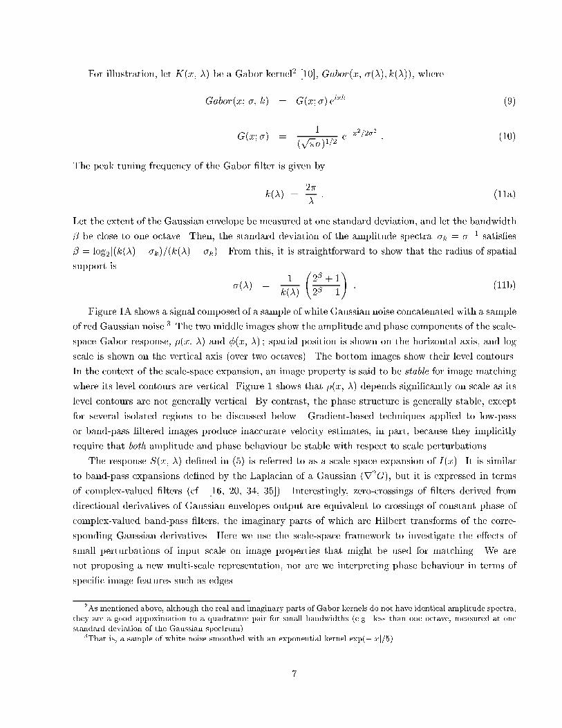
For illustration� let K�x� �� be a Gabor kernel� �� � Gabor�x� ���� k����� where

Gabor�x� � k� � G�x�� eixk ���

G�x�� �

�p�����

e�x����� � ���

The peak tuning frequency of the Gabor �lter is given by

k��� ���

�� �a�

Let the extent of the Gaussian envelope be measured at one standard deviation� and let the bandwidth

be close to one octave� Then� the standard deviation of the amplitude spectra k � �� satis�es

� log���k��� � k���k��� � k� � From this� it is straightforward to show that the radius of spatial

support is

��� �

k���

��� �

�� �

�� �b�

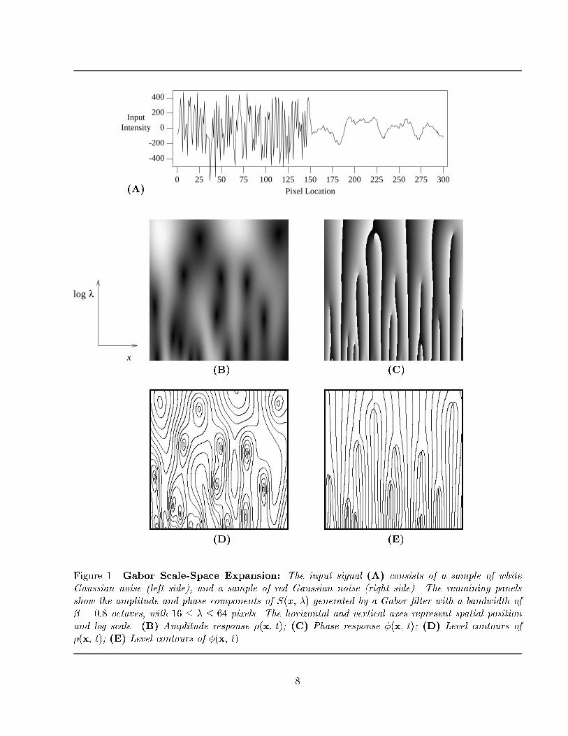
Figure A shows a signal composed of a sample of white Gaussian noise concatenated with a sample

of red Gaussian noise�� The two middle images show the amplitude and phase components of the scale�

space Gabor response� ��x� �� and ��x� �� � spatial position is shown on the horizontal axis� and log

scale is shown on the vertical axis �over two octaves�� The bottom images show their level contours�

In the context of the scale�space expansion� an image property is said to be stable for image matching

where its level contours are vertical� Figure shows that ��x� �� depends signi�cantly on scale as its

level contours are not generally vertical� By contrast� the phase structure is generally stable� except

for several isolated regions to be discussed below� Gradient�based techniques applied to low�pass

or band�pass �ltered images produce inaccurate velocity estimates� in part� because they implicitly

require that both amplitude and phase behaviour be stable with respect to scale perturbations�

The response S�x� �� de�ned in �� is referred to as a scale�space expansion of I�x�� It is similar

to band�pass expansions de�ned by the Laplacian of a Gaussian �r�G�� but it is expressed in terms

of complex�valued �lters �cf� ��� ��� ��� � �� Interestingly� zero�crossings of �lters derived from

directional derivatives of Gaussian envelopes output are equivalent to crossings of constant phase of

complex�valued band�pass �lters� the imaginary parts of which are Hilbert transforms of the corre�

sponding Gaussian derivatives� Here we use the scale�space framework to investigate the e�ects of

small perturbations of input scale on image properties that might be used for matching� We are

not proposing a new multi�scale representation� nor are we interpreting phase behaviour in terms of

speci�c image features such as edges�

�As mentioned above� although the real and imaginary parts of Gabor kernels do not have identical amplitude spectra�they are a good appoximation to a quadrature pair for small bandwidths �e�g� less than one octave� measured at onestandard deviation of the Gaussian spectrum��

�That is� a sample of white noise smoothed with an exponential kernel exp��jxj����

�

�A�0 25 50 75 100 125 150 175 200 225 250 275 300

-400

-200

0

200

400

Pixel Location

InputIntensity

x

λlog

�B� �C�

�D� �E�

Figure � Gabor Scale�Space Expansion� The input signal �A� consists of a sample of whiteGaussian noise �left side�� and a sample of red Gaussian noise �right side�� The remaining panelsshow the amplitude and phase components of S�x� �� generated by a Gabor �lter with a bandwidth of � ��� octaves� with � � � � �� pixels� The horizontal and vertical axes represent spatial positionand log scale� �B� Amplitude response ��x� t� �C� Phase response ��x� t� �D� Level contours of��x� t� �E� Level contours of ��x� t��

�

� Kernel Decomposition

The stability and linearity of phase can be examined in terms of the di�erences in phase between

an arbitrary scale�space location and other points in its neighbourhood� Towards this end� let Sj �S�xj � �j� denote the �lter response at scale�space position pj � �xj � �j�� and for convenience� let Sj

be expressed using inner products instead of convolution�

Sj � �K�j �x�� I�x�� � ���

where Kj�x� � K�xj � x� �j�� Phase di�erences in the neighbourhood of an arbitrary point p� � as a

function of relative scale�space position of neighbouring points p� � with p� � p� � ��x� ��� � can

be written as

���p�� p�� � arg�S� � arg�S� � ���

Phase is perfectly stable when �� is constant with respect to changes in scale ��� and it is linear

with respect to spatial position when �� is a linear function of �x�

To model the behaviour of S�x� �� and �� in the neighbourhood of p� we write the scale�space

response at p� in terms of S� and a residual term R�p�� p�� that goes to zero as k p��p� k� �� that

is�

S� � z�p�� p��S� � R�p�� p�� � ���

Equation ��� is easily derived if the e�ective kernel at p�� that is K��x�� is written as the sum of two

orthogonal terms� one which is a scalar multiple of K��x�� and the other orthogonal to K��x��

K��x� � z�p�� p��K��x� � H�x� p�� p�� � ��

where the complex scalar z�p�� p�� is given by

z�p� p�� � �K��x�� K��x�� � ���

and the residual kernel H�x� p�� p�� is given by

H�x� p�� p�� � K��x� � z�p�� p��K��x� � ���

Equation ��� follows from �� with R�p�� p�� � �H��x� p�� p��� I�x�� � The scalar z re�ects the

cross�correlation of the kernels K��x� and K��x�� The behaviour of R�p�� p�� is related to the signal

structure to which K��x� responds but K��x� does not�

For notational convenience below� let z� � z�p�� p��� H��x� � H�x� p�� p��� and R� � R�p�� p���

Remember that z�� H�� and R� are functions of scale�space position p� in relation to p��

�

Re

Im

R

S

z S

S1

1

1 0

0

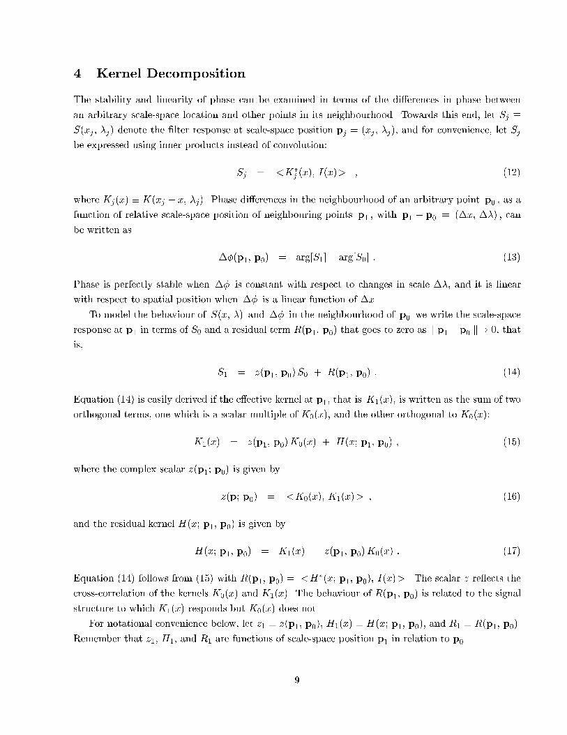
Figure �� Sources of Phase Variation� This shows the formation of S� in terms of S�� the complexscalar z� � z�p� p��� and the additive residual R� � R�p�� p���

Equation ���� depicted in Figure �� shows that the phase of S� can di�er from the phase of S�

because of the additive phase shift due to z�� and the phase shift caused by the additive residual term

R�� Phase will be stable under small scale perturbations whenever both the phase variation due to z�

as a function of scale and jR�j�jz�S�j are reasonably small� If jR�j�jz�S�j is large then phase remains

stable only when R� is in phase with S� � that is� if arg�R� � arg�S� � Otherwise� phase may vary

wildly as a function of either spatial position or small scale perturbations�

� Phase Stability Given White Gaussian Noise

To characterize the stability of phase behaviour through scale�space we �rst examine the response of

K�x� �� and its phase behaviour to stationary� white Gaussian noise� Using the kernel decomposition

��� we derive approximations to the mean phase di�erence E��� � and the variation about the mean

E� j��� E��� j � where E�� denotes mathematical expectation� The mean provides a prediction for

the phase behaviour� and the expected variation about the mean amounts to our con�dence in the

prediction� These approximations can be shown to depend only on the cross�correlation z� ���� and

are outlined below� they are derived in further detail in Appendix A�

Given white Gaussian noise� the two signals R� and z�S� are independent �because the kernels

H��x� and z�K��x� are orthogonal�� and the phase of S� is uniformly distributed over ���� � � If we

also assume that arg�R� and arg�z�S� are uncorrelated and that arg�R� � arg�z�S� is uniform� then

the residual signal R� does not a�ect the mean phase di�erence� Therefore we approximate the mean

E��� by

��z�� � arg�z� � ���

where z� is a function of scale�space position� Then� from ��� and ���� the component of �� about

�

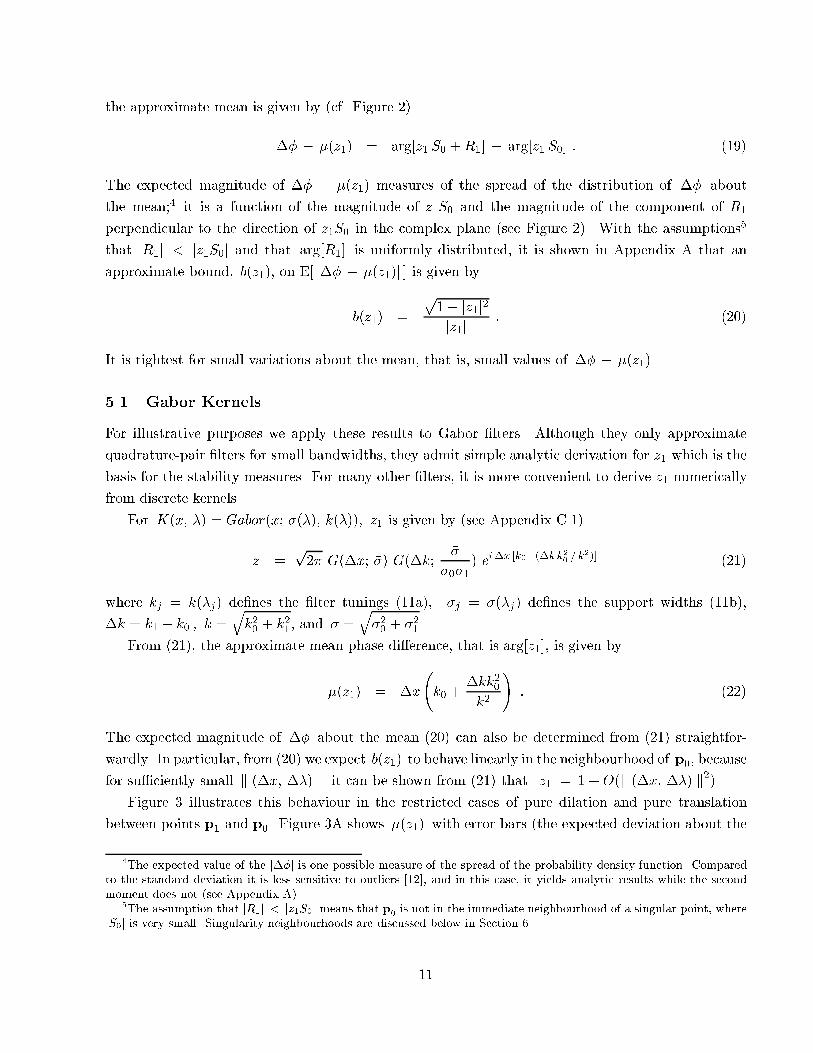
the approximate mean is given by �cf� Figure ��

�� � ��z�� � arg�z� S� �R� � arg�z� S� � ���

The expected magnitude of �� � ��z�� measures of the spread of the distribution of �� about

the mean�� it is a function of the magnitude of z�S� and the magnitude of the component of R�

perpendicular to the direction of z�S� in the complex plane �see Figure ��� With the assumptions�

that jR�j � jz�S�j and that arg�R� is uniformly distributed� it is shown in Appendix A that an

approximate bound� b�z��� on E� j�� � ��z��j is given by

b�z�� �

p� jz�j�jz�j � ����

It is tightest for small variations about the mean� that is� small values of �� � ��z�� �

��� Gabor Kernels

For illustrative purposes we apply these results to Gabor �lters� Although they only approximate

quadrature�pair �lters for small bandwidths� they admit simple analytic derivation for z� which is the

basis for the stability measures� For many other �lters� it is more convenient to derive z� numerically

from discrete kernels�

For K�x� �� � Gabor�x� ���� k����� z� is given by �see Appendix C��

z� �p�� G��x� �� G��k�

�

��� ei�x k���k k�

�� �k��� ���

where kj � k��j� de�nes the �lter tunings �a�� j � ��j� de�nes the support widths �b��

�k � k� � k� � �k �qk�� � k��� and � �

q�� � �� �

From ���� the approximate mean phase di�erence� that is arg�z� � is given by

��z�� � �x

�k� �

�kk���k�

�� ����

The expected magnitude of �� about the mean ���� can also be determined from ��� straightfor�

wardly� In particular� from ���� we expect b�z�� to behave linearly in the neighbourhood of p�� because

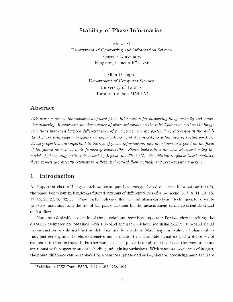
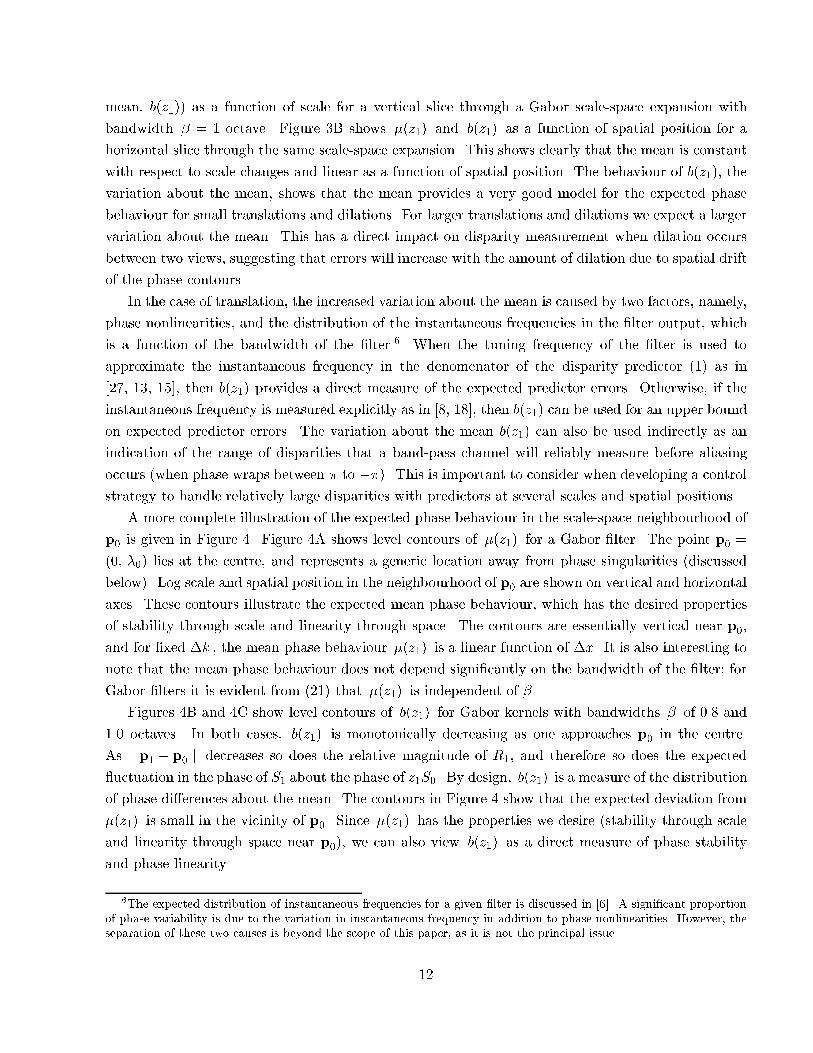
for su�ciently small k ��x� ��� k it can be shown from ��� that jz�j � �O�k ��x� ��� k���Figure � illustrates this behaviour in the restricted cases of pure dilation and pure translation

between points p� and p�� Figure �A shows ��z�� with error bars �the expected deviation about the

�The expected value of the j �j is one possible measure of the spread of the probability density function� Comparedto the standard deviation it is less sensitive to outliers ����� and in this case� it yields analytic results while the secondmoment does not �see Appendix A��

�The assumption that jR�j � jz�S�j means that p�is not in the immediate neighbourhood of a singular point� where

jS�j is very small� Singularity neighbourhoods are discussed below in Section �

mean� b�z��� as a function of scale for a vertical slice through a Gabor scale�space expansion with

bandwidth � octave� Figure �B shows ��z�� and b�z�� as a function of spatial position for a

horizontal slice through the same scale�space expansion� This shows clearly that the mean is constant

with respect to scale changes and linear as a function of spatial position� The behaviour of b�z��� the

variation about the mean� shows that the mean provides a very good model for the expected phase

behaviour for small translations and dilations� For larger translations and dilations we expect a larger

variation about the mean� This has a direct impact on disparity measurement when dilation occurs

between two views� suggesting that errors will increase with the amount of dilation due to spatial drift

of the phase contours�

In the case of translation� the increased variation about the mean is caused by two factors� namely�

phase nonlinearities� and the distribution of the instantaneous frequencies in the �lter output� which

is a function of the bandwidth of the �lter� When the tuning frequency of the �lter is used to

approximate the instantaneous frequency in the denomenator of the disparity predictor �� as in

���� �� � then b�z�� provides a direct measure of the expected predictor errors� Otherwise� if the

instantaneous frequency is measured explicitly as in ��� � � then b�z�� can be used for an upper bound

on expected predictor errors� The variation about the mean b�z�� can also be used indirectly as an

indication of the range of disparities that a band�pass channel will reliably measure before aliasing

occurs �when phase wraps between � to ���� This is important to consider when developing a control

strategy to handle relatively large disparities with predictors at several scales and spatial positions�

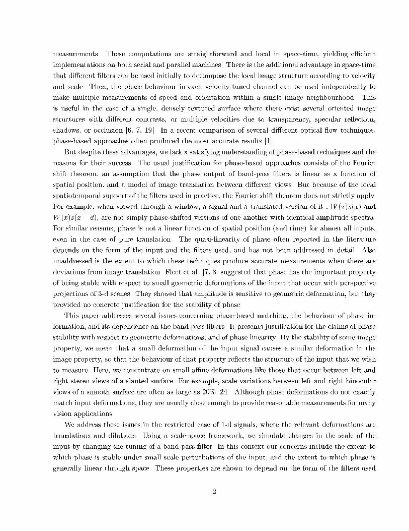
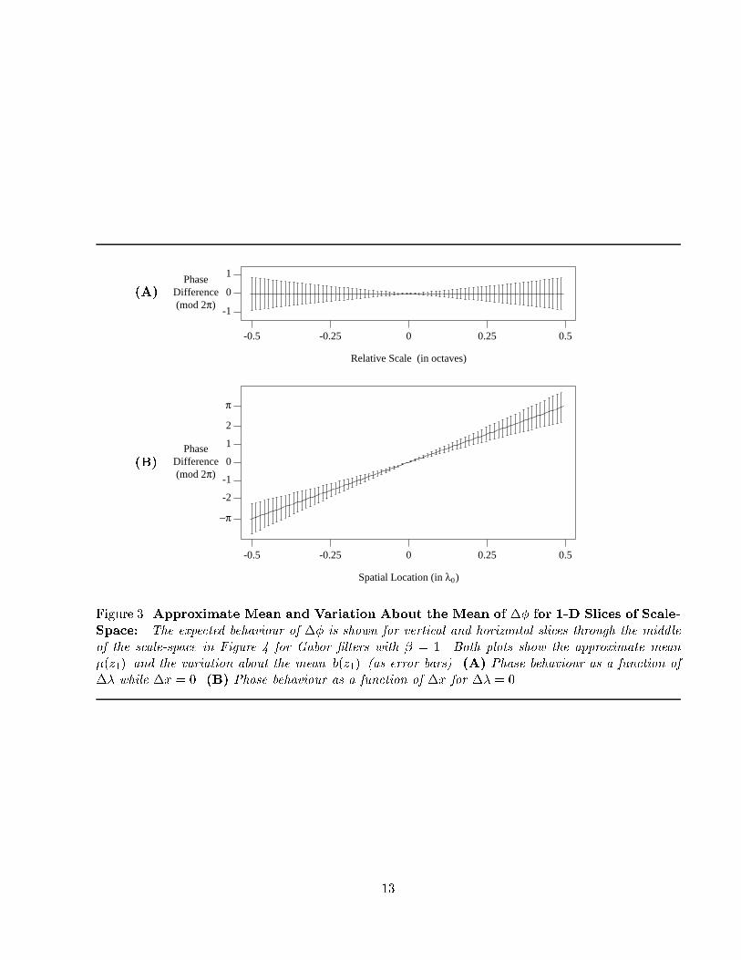
A more complete illustration of the expected phase behaviour in the scale�space neighbourhood of

p� is given in Figure �� Figure �A shows level contours of ��z�� for a Gabor �lter� The point p� �

��� ��� lies at the centre� and represents a generic location away from phase singularities �discussed

below�� Log scale and spatial position in the neighbourhood of p� are shown on vertical and horizontal

axes� These contours illustrate the expected mean phase behaviour� which has the desired properties

of stability through scale and linearity through space� The contours are essentially vertical near p��

and for �xed �k � the mean phase behaviour ��z�� is a linear function of �x� It is also interesting to

note that the mean phase behaviour does not depend signi�cantly on the bandwidth of the �lter� for

Gabor �lters it is evident from ��� that ��z�� is independent of �

Figures �B and �C show level contours of b�z�� for Gabor kernels with bandwidths of ��� and

�� octaves� In both cases� b�z�� is monotonically decreasing as one approaches p� in the centre�

As k p� � p� k decreases so does the relative magnitude of R�� and therefore so does the expected

�uctuation in the phase of S� about the phase of z�S�� By design� b�z�� is a measure of the distribution

of phase di�erences about the mean� The contours in Figure � show that the expected deviation from

��z�� is small in the vicinity of p�� Since ��z�� has the properties we desire �stability through scale

and linearity through space near p��� we can also view b�z�� as a direct measure of phase stability

and phase linearity�

�The expected distribution of instantaneous frequencies for a given �lter is discussed in ��� A signi�cant proportionof phase variability is due to the variation in instantaneous frequency in addition to phase nonlinearities� However� theseparation of these two causes is beyond the scope of this paper� as it is not the principal issue�

�

�A�

�B�

Relative Scale (in octaves)

PhaseDifference(mod 2π)

-0.5 -0.25 0 0.25 0.5

-1

0

1

Spatial Location (in λ0)

PhaseDifference(mod 2π)

-0.5 -0.25 0 0.25 0.5

−π

-2

-1

0

1

2

π

Figure �� Approximate Mean and Variation About the Mean of �� for ��D Slices of Scale�

Space� The expected behaviour of �� is shown for vertical and horizontal slices through the middleof the scale�space in Figure � for Gabor �lters with � � Both plots show the approximate mean��z�� and the variation about the mean b�z�� �as error bars�� �A� Phase behaviour as a function of�� while �x � �� �B� Phase behaviour as a function of �x for �� � ��

�

x

λlog

�A� �B� �C�

Figure �� Phase Stability with Gabor Kernels� Scale�space phase behaviour near p� � ��� ��� isshown with log scale on the vertical axis over two octaves with �� � ������ ����� and spatial positionon the horizontal axis� x� � ����� ���� The point p� is in the centres of the �gures� �A� Levelcontours ��z�� � n��� � for n � ��� ��� � �� as a function of scale�space position� These contours areindependent of the bandwidth� �B� and �C� Level contours of b�z�� are shown for � ��� and ���Each case shows the contours b�z�� � ���n where n � � ���� the innermost contours correspond tob�z�� � ��� �

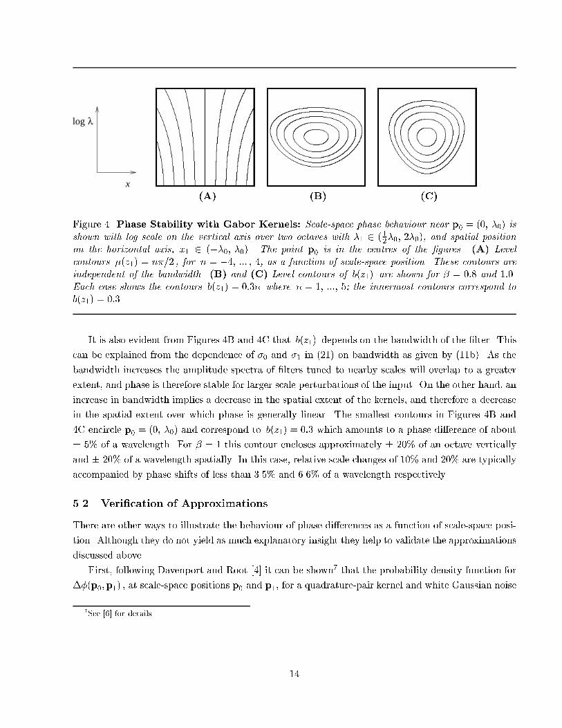
It is also evident from Figures �B and �C that b�z�� depends on the bandwidth of the �lter� This

can be explained from the dependence of � and � in ��� on bandwidth as given by �b�� As the

bandwidth increases the amplitude spectra of �lters tuned to nearby scales will overlap to a greater

extent� and phase is therefore stable for larger scale perturbations of the input� On the other hand� an

increase in bandwidth implies a decrease in the spatial extent of the kernels� and therefore a decrease

in the spatial extent over which phase is generally linear� The smallest contours in Figures �B and

�C encircle p� � ��� ��� and correspond to b�z�� � ��� which amounts to a phase di�erence of about

� � of a wavelength� For � this contour encloses approximately � ��� of an octave vertically

and � ��� of a wavelength spatially� In this case� relative scale changes of �� and ��� are typically

accompanied by phase shifts of less than ��� and ���� of a wavelength respectively�

��� Veri�cation of Approximations

There are other ways to illustrate the behaviour of phase di�erences as a function of scale�space posi�

tion� Although they do not yield as much explanatory insight they help to validate the approximations

discussed above�

First� following Davenport and Root �� it can be shown� that the probability density function for

���p��p�� � at scale�space positions p� and p�� for a quadrature�pair kernel and white Gaussian noise

�See �� for details�

�

x

λlog

�A� �B� �C�

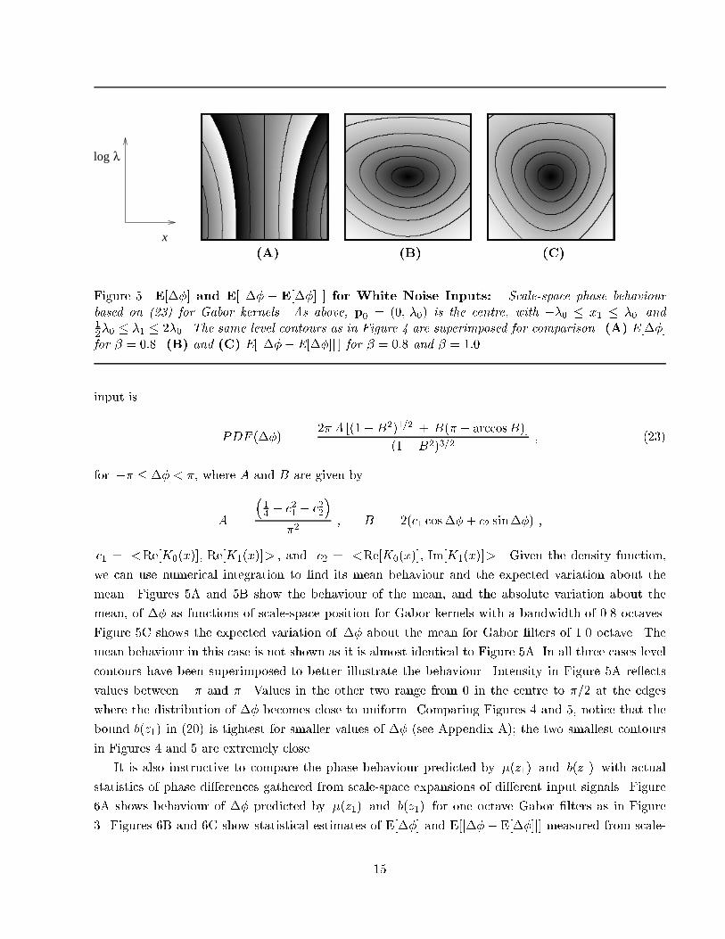
Figure � E��� and E� j�� � E��� j for White Noise Inputs� Scale�space phase behaviourbased on ���� for Gabor kernels� As above� p� � ��� ��� is the centre� with ��� � x� � �� and���� � �� � ���� The same level contours as in Figure � are superimposed for comparison� �A� E��� for � ���� �B� and �C� E� j��� E��� j for � ��� and � ���

input is

PDF ���� ��� A ���B����� � B�� � arccosB�

��B������ ����

for �� � �� � �� where A and B are given by

A �

��� � c�� � c��

���

� B � ��c� cos��� c� sin��� �

c� � �Re�K��x� � Re�K��x� � � and c� � �Re�K��x� � Im�K��x� � � Given the density function�

we can use numerical integration to �nd its mean behaviour and the expected variation about the

mean� Figures A and B show the behaviour of the mean� and the absolute variation about the

mean� of �� as functions of scale�space position for Gabor kernels with a bandwidth of ��� octaves�

Figure C shows the expected variation of �� about the mean for Gabor �lters of �� octave� The

mean behaviour in this case is not shown as it is almost identical to Figure A� In all three cases level

contours have been superimposed to better illustrate the behaviour� Intensity in Figure A re�ects

values between �� and �� Values in the other two range from � in the centre to ��� at the edges

where the distribution of �� becomes close to uniform� Comparing Figures � and � notice that the

bound b�z�� in ���� is tightest for smaller values of �� �see Appendix A�� the two smallest contours

in Figures � and are extremely close�

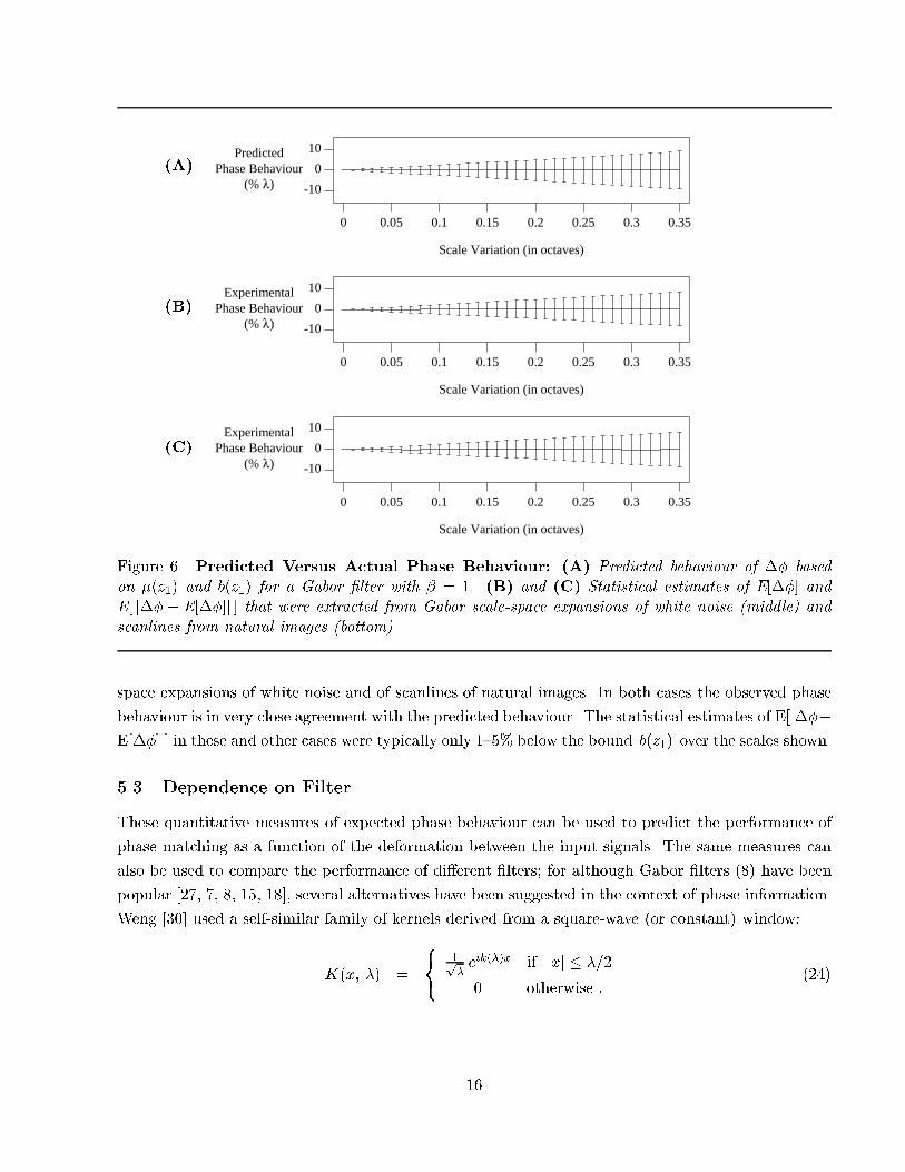
It is also instructive to compare the phase behaviour predicted by ��z�� and b�z�� with actual

statistics of phase di�erences gathered from scale�space expansions of di�erent input signals� Figure

�A shows behaviour of �� predicted by ��z�� and b�z�� for one octave Gabor �lters as in Figure

�� Figures �B and �C show statistical estimates of E��� and E�j��� E��� j measured from scale�

�A�

�B�

�C�

Scale Variation (in octaves)

PredictedPhase Behaviour

(% λ)

0 0.05 0.1 0.15 0.2 0.25 0.3 0.35

-10

0

10

Scale Variation (in octaves)

ExperimentalPhase Behaviour

(% λ)

0 0.05 0.1 0.15 0.2 0.25 0.3 0.35

-10

0

10

Scale Variation (in octaves)

ExperimentalPhase Behaviour

(% λ)

0 0.05 0.1 0.15 0.2 0.25 0.3 0.35

-10

0

10

Figure �� Predicted Versus Actual Phase Behaviour� �A� Predicted behaviour of �� basedon ��z�� and b�z�� for a Gabor �lter with � � �B� and �C� Statistical estimates of E��� andE� j�� � E��� j that were extracted from Gabor scale�space expansions of white noise �middle� andscanlines from natural images �bottom��

space expansions of white noise and of scanlines of natural images� In both cases the observed phase

behaviour is in very close agreement with the predicted behaviour� The statistical estimates of E�j���E��� j in these and other cases were typically only �� below the bound b�z�� over the scales shown�

��� Dependence on Filter

These quantitative measures of expected phase behaviour can be used to predict the performance of

phase matching as a function of the deformation between the input signals� The same measures can

also be used to compare the performance of di�erent �lters� for although Gabor �lters ��� have been

popular ���� �� �� � � � several alternatives have been suggested in the context of phase information�

Weng ��� used a self�similar family of kernels derived from a square�wave �or constant� window�

K�x� �� �

���

�p�eik���x if jxj � ���

� otherwise �����

�

x

λlog

�A� �B� �C�

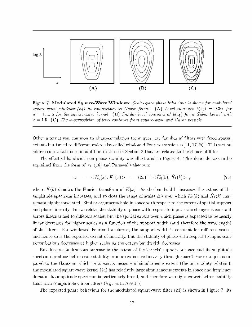
Figure �� Modulated Square�Wave Windows� Scale�space phase behaviour is shown for modulatedsquare�wave windows ���� in comparison to Gabor �lters� �A� Level contours b�z�� � ���n forn � ���� for the square�wave kernel� �B� Similar level contours of b�z�� for a Gabor kernel with � �� �C� The superposition of level contours from square�wave and Gabor kernels�

Other alternatives� common to phase�correlation techniques� are families of �lters with �xed spatial

extents but tuned to di�erent scales� also called windowed Fourier transforms �� �� �� � This section

addresses several issues in addition to those in Section � that are related to the choice of �lter�

The e�ect of bandwidth on phase stability was illustrated in Figure �� This dependence can be

explained from the form of z� ��� and Parseval�s theorem�

z� � �K��x�� K��x�� � ������ � �K��k�� �K��k�� � ���

where �K�k� denotes the Fourier transform of K�x�� As the bandwidth increases the extent of the

amplitude spectrum increases� and so does the range of scales �� over which �K��k� and �K��k� may

remain highly correlated� Similar arguments hold in space with respect to the extent of spatial support

and phase linearity� For wavelets� the stability of phase with respect to input scale changes is constant

across �lters tuned to di�erent scales� but the spatial extent over which phase is expected to be nearly

linear decreases for higher scales as a function of the support width �and therefore the wavelength�

of the �lters� For windowed Fourier transforms� the support width is constant for di�erent scales�

and hence so is the expected extent of linearity� but the stability of phase with respect to input scale

perturbations decreases at higher scales as the octave bandwidth decreases�

But does a simultaneous increase in the extent of the kernels� support in space and its amplitude

spectrum produce better scale stability or more extensive linearity through space For example� com�

pared to the Gaussian which minimizes a measure of simultaneous extent �the uncertainty relation��

the modulated square�wave kernel ���� has relatively large simultaneous extents in space and frequency

domain� Its amplitude spectrum is particularly broad� and therefore we might expect better stability

than with comparable Gabor �lters �e�g�� with � ���

The expected phase behaviour for the modulated square�wave �lter ���� is shown in Figure �� Its

�

mean phase behaviour� given by arg�z� � is very much like that exhibited by Gabor �lters in Figure �A

and is not shown� Figure �A shows the scale�space behaviour of b�z�� for the modulated square�wave

kernel ����� for which z� is given by �see Appendix C���

z� � i ei�xk��ei�k a� � ei�k a�

���k

p�����

�� � ����

where �� and �k are de�ned above�� and

a� �����

�max

��� ���

���x

�� a� �

���

�min

���

��

���x

��

For comparison� Figure �B shows level contours of b�z�� for a Gabor kernel with a bandwidth of

� �� and Figure �C shows the superposition of the level contours from Figures �A and �B� These

�gures show that the distribution of �� about the mean for the modulated suare�wave kernel is two

to three times larger near p�� which suggests poorer stability and poorer linearity� Note that the

innermost contour of the Gabor �lter clearly encloses the innermost contour of the square�wave �lter�

This Gabor �lter handles scale perturbations of �� with an expected phase drift of up to � ���� of

a wavelength� while a perturbation of �� for the modulated square�wave kernels gives b�z�� � ���� �

which amounts to a phase di�erence of about �����

The poorer phase stability exhibited by the modulated square�wave kernel implies a wider distri�

bution of measurement errors� Because of the phase drift due to scale changes� even with perfect phase

matching� the measurements of velocity and disparity will not re�ect the projected motion �eld and

the projected disparity �eld as reliably� The poorer phase linearity a�ects the accuracy and speed of

the disparity predictor� requiring more iterations to match the phase values between views� Moreover�

we �nd that the larger variance also causes a reduction in the range of disparities that can be measured

reliably from the predictor� The poorer linearity exhibited in Figure � also contradicts a claim in ���

that modulated square�wave �lters produce more nearly linear phase behaviour�

Wider amplitude spectra do not necessarily ensure greater phase stability� Phase stability is the

result of correlation between kernels at di�erent scales� The shapes of both the amplitude and phase

spectra will therefore play signi�cant roles� The square�wave amplitude spectra is wide� but with

considerable ringing so that jz�j falls o� quickly with small scale changes�

Another issue concerning the choice of �lter is the ease with which phase behaviour can be ac�

curately extracted from a subsampled encoding of the �lter output� It is natural that the outputs

of di�erent band�pass �lters be quantized and subsampled to avoid an explosion in the number of

bits needed to represent �ltered versions of the input� However� because of the aliasing inherent in

subsampled encodings� care must be taken in subsequent numerical interpolation�di�erentiation� For

example� we found that� because of the broad amplitude spectrum of the modulated square�wave and

its sensitivity to low frequencies� sampling rates had to be at least twice as high as those with Gabors

�with comparable bandwidths� � �� to obtain reasonable numerical di�erentiation� If these issues

�As k� �� this expression for z� converges to exp�i xk�� ��� x�����

�

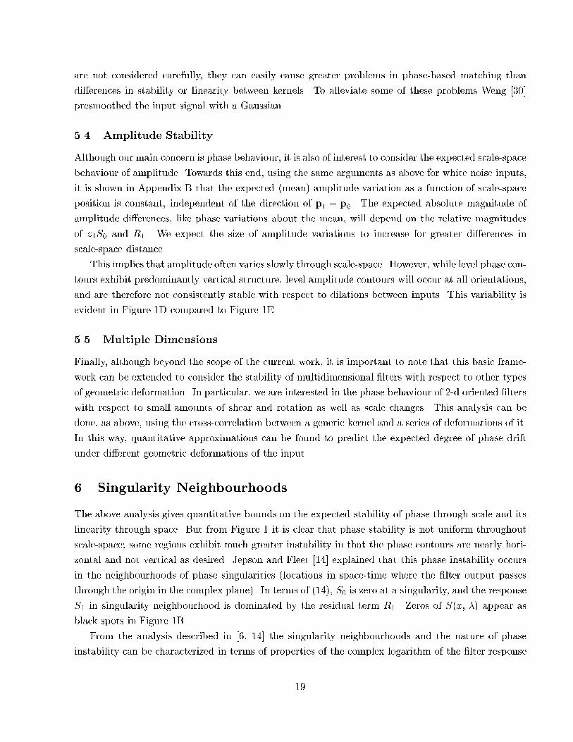
are not considered carefully� they can easily cause greater problems in phase�based matching than

di�erences in stability or linearity between kernels� To alleviate some of these problems Weng ���

presmoothed the input signal with a Gaussian�

��� Amplitude Stability

Although our main concern is phase behaviour� it is also of interest to consider the expected scale�space

behaviour of amplitude� Towards this end� using the same arguments as above for white noise inputs�

it is shown in Appendix B that the expected �mean� amplitude variation as a function of scale�space

position is constant� independent of the direction of p� � p�� The expected absolute magnitude of

amplitude di�erences� like phase variations about the mean� will depend on the relative magnitudes

of z�S� and R�� We expect the size of amplitude variations to increase for greater di�erences in

scale�space distance�

This implies that amplitude often varies slowly through scale�space� However� while level phase con�

tours exhibit predominantly vertical structure� level amplitude contours will occur at all orientations�

and are therefore not consistently stable with respect to dilations between inputs� This variability is

evident in Figure D compared to Figure E�

��� Multiple Dimensions

Finally� although beyond the scope of the current work� it is important to note that this basic frame�

work can be extended to consider the stability of multidimensional �lters with respect to other types

of geometric deformation� In particular� we are interested in the phase behaviour of ��d oriented �lters

with respect to small amounts of shear and rotation as well as scale changes� This analysis can be

done� as above� using the cross�correlation between a generic kernel and a series of deformations of it�

In this way� quantitative approximations can be found to predict the expected degree of phase drift

under di�erent geometric deformations of the input�

� Singularity Neighbourhoods

The above analysis gives quantitative bounds on the expected stability of phase through scale and its

linearity through space� But from Figure it is clear that phase stability is not uniform throughout

scale�space� some regions exhibit much greater instability in that the phase contours are nearly hori�

zontal and not vertical as desired� Jepson and Fleet �� explained that this phase instability occurs

in the neighbourhoods of phase singularities �locations in space�time where the �lter output passes

through the origin in the complex plane�� In terms of ���� S� is zero at a singularity� and the response

S� in singularity neighbourhood is dominated by the residual term R�� Zeros of S�x� �� appear as

black spots in Figure B�

From the analysis described in ��� � the singularity neighbourhoods and the nature of phase

instability can be characterized in terms of properties of the complex logarithm of the �lter response

�

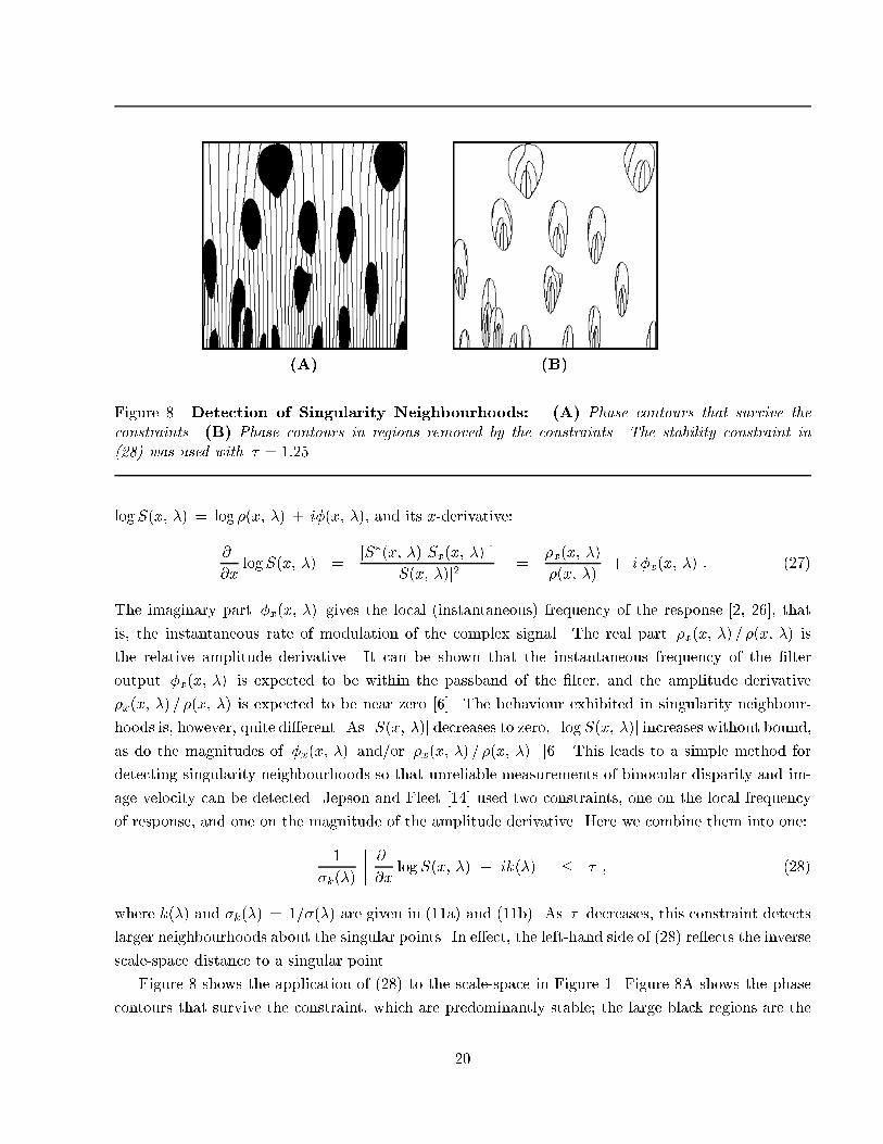
�A� �B�

Figure �� Detection of Singularity Neighbourhoods� �A� Phase contours that survive theconstraints� �B� Phase contours in regions removed by the constraints� The stability constraint in���� was used with � � �� �

log S�x� �� � log ��x� �� � i��x� ��� and its x�derivative�

xlogS�x� �� �

�S��x� �� Sx�x� ��

jS�x� ��j� ��x�x� ��

��x� ��� i �x�x� �� � ����

The imaginary part �x�x� �� gives the local �instantaneous� frequency of the response ��� �� � that

is� the instantaneous rate of modulation of the complex signal� The real part �x�x� �� � ��x� �� is

the relative amplitude derivative� It can be shown that the instantaneous frequency of the �lter

output �x�x� �� is expected to be within the passband of the �lter� and the amplitude derivative

�x�x� �� � ��x� �� is expected to be near zero �� � The behaviour exhibited in singularity neighbour�

hoods is� however� quite di�erent� As jS�x� ��j decreases to zero� j log S�x� ��j increases without bound�

as do the magnitudes of �x�x� �� and�or �x�x� �� � ��x� �� �� � This leads to a simple method for

detecting singularity neighbourhoods so that unreliable measurements of binocular disparity and im�

age velocity can be detected� Jepson and Fleet �� used two constraints� one on the local frequency

of response� and one on the magnitude of the amplitude derivative� Here we combine them into one�

k���

x log S�x� �� � ik���

� � � ����

where k��� and k��� � ���� are given in �a� and �b�� As � decreases� this constraint detects

larger neighbourhoods about the singular points� In e�ect� the left�hand side of ���� re�ects the inverse

scale�space distance to a singular point�

Figure � shows the application of ���� to the scale�space in Figure � Figure �A shows the phase

contours that survive the constraint� which are predominantly stable� the large black regions are the

��

singularity neighbourhoods detected by ����� Figure �B shows those removed by the constraint� which

amounts to about ��� of the entire scale�space area� With respect to the quantitative approximations

to phase behaviour presented in Section �� we reported that statistics of mean phase di�erences and

the absolute variation about the mean agreed closely with the bounds� When the phase behaviour in

singularity neighbourhoods is ignored� so that the statistics are gathered only from outside of such

singularity neighbourhoods� we �nd that the magnitude of the variation of �� about the mean is

generally less than half of that predicted by the bound in ����� This detection of unstable regions

is essential to the reliable performance of phase�based matching techniques� and it can be used to

improve the performance of zero�crossing and phase�correlation techniques �� �� �� ��� �� �

� Natural Images

Unlike white noise� the Fourier harmonics of natural images are often correlated across scales� and

their amplitude spectra typically decay something like �k � � Both of these facts a�ect our re�

sults concerning phase stability� the accuracy of phase matching� and instability due to singularity

neighbourhoods�

First� because of amplitude spectra decay with spatial frequency� the �lter responses will be biased

to lower frequencies �as compared to white noise�� As a result� care is required to ensure that the

�lter outputs do not contain too much power at low frequencies� Otherwise� there may be a� more

distortion due to aliasing in a subsampled representation of the response� and b� larger singularity

neighbourhoods� and hence a sparser set of reliable measurements� These problems are evident when

comparing the modulated square�wave �lters with Gabor �lters �or similar bandwidths� because the

former have greater sensitivity to low frequencies� Second� without the assumption of white noise we

should expect z� S� and R� in ��� to be correlated� This will lead to improved phase stability when

R� and S� remain in phase� and poorer stability when they become systematically out of phase�

Although we lack a su�cient model of natural images� in terms of local structure� to provide a

detailed treatment of phase stability on general images� several observations are readily available� For

example� with many textured image regions the phase structure appears much like that in Figure

� We �nd that the noise�based analysis provides a good model of the expected phase behaviour for

complex structures that regularly occur in natural images�

Moreover� it appears that phase is even more stable in the neighbourhoods of salient image features�

such as those that occur in man�made environments� To see this� note that the output of a �lter in a

small region can be viewed as a weighted sum of harmonics� In the vicinity of localized image features

such as edges� bars and ramps� we expect greater phase stability because the phases of the input

harmonics �unlike the white noise� are already coincident� This is clear from their Fourier transforms�

Therefore changing scales slightly� or adding new harmonics at the high or low ends of the passband

will not change the phase of the output signi�cantly�

It is also worth noting that this phase coincidence at the feature locations coincides with local

maxima of the amplitude response ��� � When di�erent harmonics are in phase their amplitudes

�

combine additively� When out of phase they cancel� Therefore it can be argued that neighbourhoods

of local amplitude maxima correspond to regions in which phase is maximally stable �as long as

the signal�to�noise�ratio is su�ciently high�� This is independent of the absolute phase at which the

di�erent harmonics coincide�� and is signi�cant for stable phase�based matching�

As one moves away from salient features� such as edges� the di�erent harmonics may become

increasingly out of phase� the responses from di�erent features may interfere� and the amplitude of

response decreases� This yields two main types of instability� �� where interference from nearby

features causes the total response to disappear at isolated points� and �� where large regions have

very small amplitude and are dominated by noise� The �rst case amounts to a phase singularity and

is detectable using the stability constraint ����� In the second case� the phase behaviour in di�erent

views may be dominated by uncorrelated noise� but will not necessarily violate the stability constraint�

For these situations a signal�to�noise constraint is necessary�

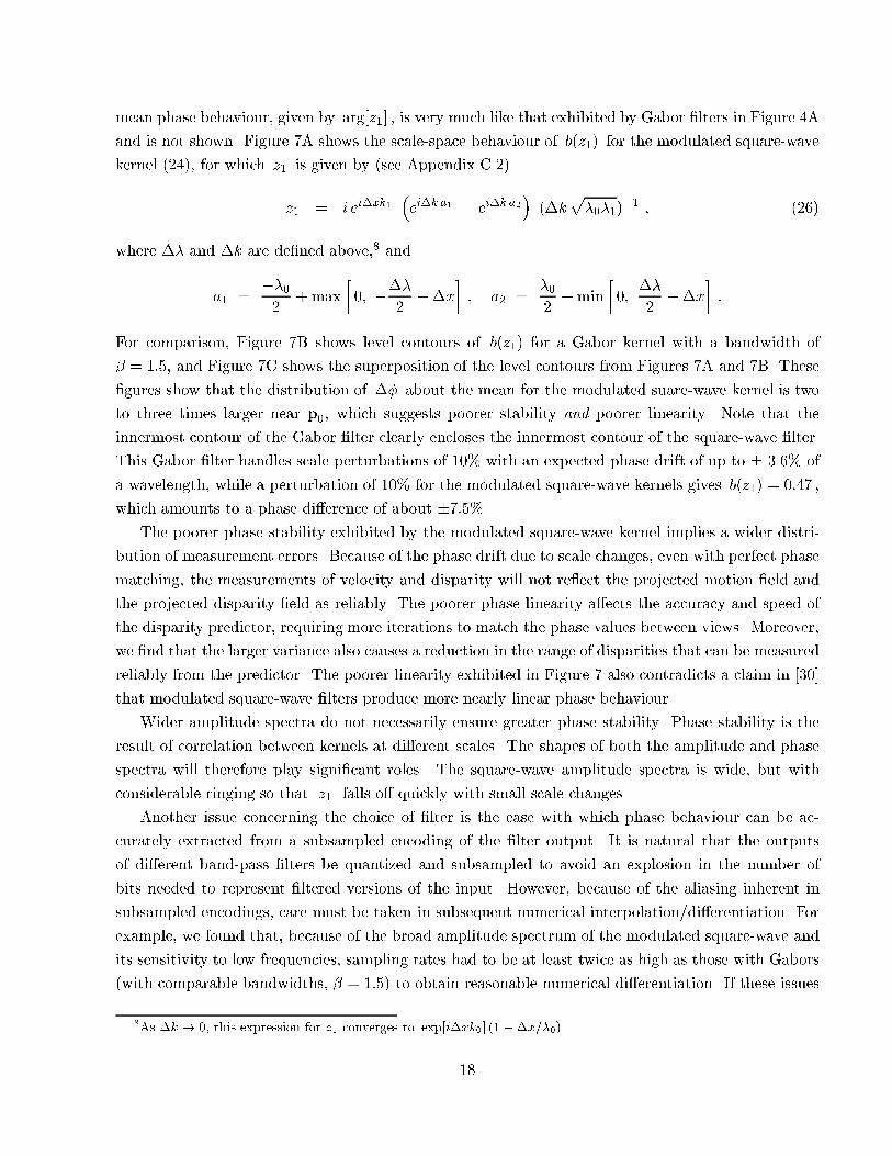
To illustrate these points� Figure � shows the Gabor scale�space expansion of a signal containing

several step edges �Figure �A�� There are two bright bars� �� and � pixels wide� � pixels apart�

The scale�space plots were generated by Gabor �lters with � � spanning � octaves � � � � � ����

Figures �A and �B show the amplitude response and its level contours superimposed on the input

signal �replicated through scale� to show the relationship between amplitude variation and the edges�

Figures �C and �D show the scale�space phase response and its level contours� and Figures �E and

�F show the contours that remain after the detection of singularity neighbourhoods using ���� with

� � ��� and the phase contours in the neighbourhoods detected by ����� As expected� phase is stable

near the edge locations where the local Fourier harmonics are in phase� and arg�R� � arg�S� over

a wide range of scales� The similarity of the interference patterns between the di�erent edges to the

singularity neighbourhoods shown in Figures and � is clear� and these regions are detected using the

stability constraint� Also detected are the regions relatively far from the edges where the amplitude

and phase responses of the �lter both go to zero�

However� as explained above� regions in which the �lter response decreases close to zero are also

very sensitive to noise� These regions can become di�cult to match since uncorrelated noise between

two views can dominate the response� To illustrate this� we generated a di�erent version of the scale�

space in which uncorrelated noise was added to the input independently before computing each scale

�to simulate uncorrelated noise added to di�erent views�� The response to the independent noise

patterns satis�ed the stability constraint much of the time� but the phase structure was unstable

�uncorrelated� between scales� Figure �H shows the regions detected by the stability constraint in this

case� As discussed� the regions of low amplitude in the original are now dominated by the response to

the noise and are no longer detected by ����� Another constraint on the signal�to�noise ratio of the

�lter output appears necessary� For example� Figure �I shows the regions in which the amplitude of

the �lter output is � or less of the maximum amplitude at that scale� This constraint in conjunction

Morrone and Burr ���� argue that psychophysical salience �of spatial features� correlates well with phase coincidenceonly for certain absolute values of phase� namely� integer multiples of ���� which are perceived as edges and bars ofdi�erent polarities�

��

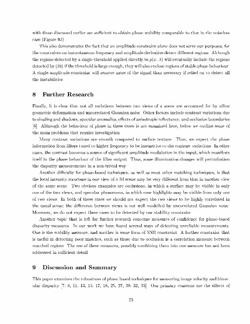
with those discussed earlier are su�cient to obtain phase stability comparable to that in the noiseless

case �Figure �J��

This also demonstrates the fact that an amplitude constraint alone does not serve our purposes� for

the constraints on instantaneous frequency and amplitude derivative detect di�erent regions� Although

the regions detected by a single threshold applied directly to ��x� �� will eventually include the regions

detected by ���� if the threshold is large enough� they will also enclose regions of stable phase behaviour�

A single amplitude constraint will remove more of the signal than necessary if relied on to detect all

the instabilities�

� Further Research

Finally� it is clear that not all variations between two views of a scene are accounted for by a�ne

geometric deformation and uncorrelated Gaussian noise� Other factors include contrast variations due

to shading and shadows� specular anomalies� e�ects of anisotropic re�ectance� and occlusion boundaries

�� � Although the behaviour of phase in these cases is not examined here� below we outline some of

the main problems that require investigation�

Many contrast variations are smooth compared to surface texture� Thus� we expect the phase

information from �lters tuned to higher frequency to be insensitive to the contrast variations� In other

cases� the contrast becomes a source of signi�cant amplitude modulation in the input� which manifests

itself in the phase behaviour of the �lter output� Thus� some illumination changes will perturbation

the disparity measurements in a non�trivial way�

Another di�culty for phase�based techniques� as well as most other matching techniques� is that

the local intensity structure in one view of a �d scene may be very di�erent from that in another view

of the same scene� Two obvious examples are occlusions� in which a surface may be visible in only

one of the two views� and specular phenomena� in which case highlights may be visible from only one

of two views� In both of these cases we should not expect the two views to be highly correlated in

the usual sense� the di�erence between views is not well modelled by uncorrelated Gaussian noise�

Moreover� we do not expect these cases to be detected by our stability constraint�

Another topic that is left for further research concerns measures of con�dence for phase�based

disparity measures� In our work we have found several ways of detecting unreliable measurements�

One is the stability measure� and another is some form of SNR constraint� A further constraint that

is useful in detecting poor matches� such as those due to occlusion is a correlation measure between

matched regions� The use of these measures� possibly combining them into one measure has not been

addressed in su�cient detail�

Discussion and Summary

This paper examines the robustness of phase�based techniques for measuring image velocity and binoc�

ular disparity ��� �� � �� � �� �� �� ��� ��� ��� �� � Our primary concerns are the e�ects of

��

�A� 0 25 50 75 100 125 150 175 200

0

100

200

Pixel Location

InputIntensity

�B� �C� �D�

�E� �F� �G�

�H� �I� �J�

Figure �� Gabor Scale�Space Expansion With Step�Edge Input� The input signal �A� consistsof two bars� Vertical and horizontal axes of the Gabor scale�space represent log scale and spatialposition� Level contour have been superimposed on the input to show the relative location of the edges��B� and �C� ��x� �� and its level contours �D� and �E� ��x� �� and its level contours �F� and �G�Level phase contours that survive the stability constraint ����� and those detected by it �H� Regionsof the �noisy�scale�space� that were detected by ���� �I� Regions detected by a simple amplitudeconstraint �J� The level phase contours that survive the union of constraints in �H� and �I����

the �lters and the stability of phase with respect to typical image deformations that occur between

di�erent views of ��d scenes� Using a scale�space framework it was shown that phase is generally

stable with respect to small scale perturbations of the input� and quasi�linear as a function of spatial

position� Quantitative measures of the expected phase stability and phase linearity were derived for

this purpose� From this it was shown that both phase stability and linearity depend on the form of

the �lters and their frequency bandwidths� For a given �lter type� as the bandwidth increases� the

extent of the phase stability increases� while the spatial extent over which phase is expected to be

linear decreases� In the context of disparity measurement� the bandwidth of the �lters should therefore

depend� in part� on the expected magnitude of deformation between left and right views� since the

potential accuracy of phase�based matching depends directly on phase stability�

One of the main causes of instability is the occurrence of phase singularities� the neighbourhoods of

which exhibit phase behaviour that is extremely sensitive to input scale perturbations� small changes

in spatial position� and small amounts of noise� Phase behaviour in these neighbourhoods is a source of

signi�cant measurement error for phase�di�erence and phase�gradient techniques� as well as gradient�

based techniques� zero�crossing techniques� and phase�correlation techniques� Fortunately� singularity

neighbourhoods can be detected automatically using a simple constraint ���� on the �lter output�

This stability constraint is an essential component of phase�based methods� A second constraint is

also needed to ensure a reasonable signal�to�noise ratio�

This basic approach can also be used to examine the stability of multi�dimensional �lters to other

types of geometric deformation� such as the stability of ��d oriented �lters with respect to local a�ne

deformation �rotation� shear� and dilation�� As explained here� we may consider the behaviour of

phase information using the cross�correlation of deformed �lter kernels z� as a function of rotation

and shear in addition to the case of dilation on which we concentrated in this paper� In this way�

quantitative approximations can be found to predict the expected degree of phase drift under di�erent

geometric deformations of the input�

Acknowledgements

We are grateful to Michael Langer for useful comments on earlier drafts of this work� This research

has been supported in part by the Natural Sciences and Engineering Research Council of Canada� and

the Ontario Government under the ITRC centres�

References

� Barron� J�L�� Fleet� D�J�� Beauchemin� S�� and Burkitt� T� ����� Performance of optical �ow

techniques� Proc� IEEE CVPR� Champaign� pp� ������� �also see Technical Report RPL�TR�

���� Department of Computing Science� Queen�s University�

�� Boashash� B� ����� Estimating and interpreting the instantaneous frequency of a signal� Proc�

IEEE ��� pp� �����

�

�� Burt� P�J�� Bergen� J�R�� Hinhorani� R�� Kolczynski� R�� Lee� W�A�� Leung� A�� Lubin� J�� and

Shvaytser� H� ����� Object tracking with a moving camera� Proc� IEEE Workshop on Visual

Motion� Irvine� pp� ����

�� Davenport� W�B� and Root� W� ���� Introduction to the Theory of Random Signals and Noise�

McGraw�Hill� New York

� Field� D�J� ����� Relations between the statistics of natural images and the response properties

of cortical cells� J� Opt� Soc� Am� A �� pp� ���������

�� Fleet� D�J� ����� Measurement of Image Velocity� Kluwer Academic Publishers� Norwell MA

�� Fleet� D�J� and Jepson� A�D� ����� Computation of component image velocity from local phase

information� Int� J� Computer Vision � pp� �����

�� Fleet� D�J�� Jepson� A�D� and Jenkin� M� ���� Phase�based disparity measurement� CVGIP�

Image Understanding �� pp� �����

�� Freeman� W�T� and Adelson� E�H� ���� The design and use of steerable �lters� IEEE Trans�

PAMI �� pp� ������

�� Gabor� D� ����� Theory of communication� J� IEE ��� pp� ������

� Girod� B� and Kuo� D� ����� Direct estimation of displacement histograms� Proc� OSA Topcial

Meeting on Image Understanding and Machine Vision� pp� ������ Cape Cod

�� Huber� P�J� ���� Robust Statistics� John Wiley ! Sons� New York

�� Jenkin� M�� and Jepson� A�D� ����� The measurement of binocular disparity� in Computational

Proceses in Human Vision� �ed�� Z� Pylyshyn� Ablex Press� New Jersey

�� Jepson� A�D� and Fleet� D�J� ���� Phase singularities in scale�space� Image and Vision Com�

puting �� pp� �������

� Jepson� A�D� and Jenkin� M� ����� Fast computation of disparity from phase di�erences� Proc�

IEEE CVPR� San Diego� pp� �������

�� Koenderink� J�J� ����� The structure of images� Biological Cybernetics �� pp� �������

�� Kuglin� C� and Hines� D� ���� The phase correlation image alignment method� Proc� IEEE Int�

Conf� Cybern� Society� pp� ����

�� Langley� K�� Atherton� T�J�� Wilson� R�G�� and Larcombe� M�H�E� ����� Vertical and horizontal

disparities from phase� Proc� �st ECCV� Antibes� Springer�Verlag� pp� ����

�� Langley� K�� Fleet� D�J�� and Atherton� T� ����� Multiple motion from instantaneous frequency�

Proc� IEEE CVPR� Champaign� pp� �������

��

��� Mallat� S�G� ����� Multifrequency channel decomposition of images and wavelet models� IEEE

Trans� ASSP ��� pp� ������

�� Marr� D� and Poggio� T� ����� A computational theory of human stereo vision� Proc� R� Soc�

Lond� B���� pp� ������

��� Mayhew� J� and Frisby� J� ���� Computational studies toward a theory of human stereopsis�

Arti�cial Intelligence �� pp ������

��� Morrone� M�C� and Burr� D�C� ����� Feature detection in human vision� a phase�dependent

energy model� Proc� R� Soc� Lond� B ��� pp� �����

��� Ogle� K�N� ���� Research in Binocular Vision� W�B� Saunders Co�� Philadelphia

�� Olson� T� and Potter� R� ����� Real�time vergence control� Proc� IEEE CVPR� San Diego� pp�

�������

��� Papoulis� A� ���� Probability� Random Variables� and Stochastic Processes� McGraw�Hill� New

York

��� Sanger� T� ����� Stereo disparity computation using Gabor �lters� Biological Cybernetics �� pp�

�����

��� Simoncelli� E�P�� Freeman� W�T�� Adelson� E�H� and Heeger� D�J� ����� Shiftable multiscale

transforms� IEEE Trans� Info� Theory ��� pp� ������

��� Waxman� A�M�� Wu� J�� and Bergholm� F� ����� Convected activation pro�les� Receptive �elds

for real�time measurement of short�range visual motion� Proc� IEEE CVPR� Ann Arbor� pp�

������

��� Weng� J� ����� A theory of image matching� Proc� �rd ICCV� Osaka� pp� �������

�� Westelius� C�J ����� Preattentive gaze control for robot vision� Thesis� LIU�TEK�LIC�������

Dept� of Electrical Engineering� Linkoping University� Sweden

��� Wiklund� J�� Westelius� C�J� and Knuttson� H� ����� Hierarchical phase�based disparity estima�

tion� Technical Report� LiTH�ISY�I����� Dept� of Electrical Engineering� Linkoping University�

Sweden

��� Wilson� R� and Knuttson� H� ����� A multiresolution stereopsis algorithm based on the Gabor

representation� Proc� IEE Intern� Conf� Im� Proc� and Applic�� Warwick� U�K�� pp� ����

��� Witkin� A�P� ����� Scale�space �ltering� Proc� �th IJCAI� Karlsruhe� pp� ������

�� Yuille� A�L� and Poggio� T�A� ����� Scaling theorems for zero�crossings� IEEE Trans� PAMI ��

pp� ��

��

A Approximations to Expected Phase Behaviour

This appendix provides greater detail about the approximations used in Sections � and to illus�

trate and predict scale�space phase behaviour� In particular� it derives approximations to E��� and

E� j�� � E��� j where� as de�ned in Section �� ���p�� p�� is the phase di�erence between two

points in scale�space� We are interested in the behaviour of ���p�� p�� as a function of points p�

in the neighbourhood of an arbitrary point p� �away from the immediate neighbourhoods of singular

points��

Following the notation in Section �� let Kj�x� and Sj be the e�ective kernel and its response

at scale�space location pj� We assume that Kj�x� is a quadrature�pair kernel� Then� using the

decompositions in ��� and �� we can write the response at S� as

S� � z� S� � R� � ����

where z��p�� p�� � �K��x�� K��x�� and R� is the response to the residual kernel H��x� de�ned by

���� If we suppose a random process for the input� then� ���� speci�es how the random variable S�

is derived from the known quantity z�� and the random variables S� and R�� In this way we can also

relate the phase of S� to the phase of S��

For mean�zero Gaussian white�noise input� the response S� is mean�zero Gaussian with variance

�� � k K� k� � ��� and assuming that K� is a quadrature �lter the real and imaginary parts of S�

have a joint Gaussian density� with zero mean and a isotropic covariance � � �� �Papoulis� �� �

The phase of S� is uniformly distributed over ���� � and independent of the amplitude� Based on

similar arguments� z� S� is also mean�zero Gaussian� but its variance is jz�j�� and that of its real and

imaginary parts is jz�j��� and isotropic� In polar coordinates� �� � jz� S�j has a Rayleigh density

with mean E��� �p� jz�j��� and second moment E���� � jz�j�� where E�� denotes mathematical

expectation� Its phase angle �� � arg�z� S� is independent of �� and has a uniform density function

�Papoulis� �� �

The real and imaginary parts of the residual process R� are Gaussian� But their density is not

isotropic with uniform phase because the real and imaginary parts of the kernel H��x� are not orthog�

onal� To see this� note that

�Re�H��x� � Im�H��x� � � � Im��K�� �x� � z�K��x�� � ����

which is generally non�zero� ���� follows from the fact that �Re�z�K� � Im�z�K� � and �Re�K� � Im�K� �

are both �� As an approximation we assume that H��x� is a quadrature �lter so that its output is

mean�zero with variance �� � k H��x� k�� In other words� we assume that �� � jR�j has a Rayleigh

density with mean E��� �p� k H��x� k��� and second moment E���� � k H��x� k�� Its phase angle

�� � arg�R� is independent of �� and has a uniform density function over ���� � � These expressions

��Given stationary white noise the spectral density of the output equals the power spectrum of the �lter�

��

can be simpli�ed further because k H��x� k can be shown to reduce top� jz�j� � This is easily

derived from H��x� � K��x� � z�K��x� as follows�

k H��x� k� � �K��x�� z�K��x�� K��x�� z�K��x��

� k K��x� k� � k z�K��x� k� � ��z�K��x�� K��x�� � �K��x�� z�K��x�� �

� � jz�j� � ��z�K��x�� K��x�� � �z�K��x�� K��x����

� � jz�j� � �Re�z�� �K��x�� K��x��

� � jz�j� � ���

Finally� because the kernels z�K��x� and H��x� are orthogonal �by construction� the two signals

z� S� and R� are uncorrelated� and because the input is Gaussian they are statistically independent�

With the assumption that R� is isotropic in its real and imaginary parts� it has no in�uence on the

mean phase di�erence �� � arg�S� � arg�S� � Thus� we approximate E��� by ��z�� � arg�z� � By

the same argument� the variation of �� about the mean is determined by the phase di�erence between

z� S� and S� � z� S� �R�� that is

��� ��z�� � �arg�S� � arg�S� � � arg�z�

� arg�z� S� �R� � arg�z� S� � ����

When jR�j � jz� S�j �i�e� with p� not in the immediate neighbourhood of a phase singularity�� the

magnitude of ��� ��z�� is given by the magnitude of the arctangent of the component of R� that

is perpendicular to the complex direction of z�S�� divided by the magnitude of z�S� �cf� Figure ���

that is�

j��� ��z��j �arctan

d���

� � jd�j��

� ����

where �� � jz� S�j� and

d� �Im��z� S��

�R�

jz� S�j � Im�e�i�� R� � �� Im�ei������� � ����

where �� � arg�z� S� and R� � �� ei�� � Viewed as vectors in the complex plane� d� is the length of

the projection of R� onto the unit vector normal to z�S�� Finally� we can now formulate a bound on

E� j��� ��z��j as follows

E� j��� ��z��j � E

� jd�j��

�� E����� E��� E� j sin��� � ���j � ���

This follows from the independence of the four random quantities ��� ��� ��� and ��� From above�

we know that E��� �p� k H��x� k�� ��

p��� jz�j����� Moreover� given the Rayleigh densities

of �� and ��� and the uniform densities of �� and �� � it can be shown that E����� �p� � jz�j and

��

E� j sin��� � ���j � ��� � Therefore� the bound reduces to

E� j��� ��z��j �p � jz�j�jz�j � ����

It is tightest for small values of ��� ��z�� because of the bound used in �����

B Approximations to Expected Amplitude Behaviour

Using the same arguments as Appendix A� it can be shown that the expected �mean� amplitude

variation as a function of scale�space position is constant� independent of the direction of p� �p�� To

see this� we �rst rewrite ���� in terms of the amplitude and phase components of z�S� and R�

S� � jz�j��ei�� � ��ei�� � ����

where �� � arg�z�S� � �� � jS�j� �� � arg�R� � and �� � jR�j� With straightforward algebraic

manipulation� the squared magnitude of S� can be written as

jS�j� � jz�j� ��� � ��� � �jz�j ���� cos��� � ��� � ����

As above� ���� expresses the magnitude of S� as a function of known quantities and random

variables� Its expected value is

E� jS�j� � jz�j�E� ��� � E� ��� � �jz�jE� ���� cos��� � ��� � ����

Using the same facts and assumptions as in Appendix A �i�e�� the assumptions of white Gaussian

input� the independence of variables ��� ��� ��� and ��� and the uniformity of �� � ��� equation ����

becomes

E� jS�j� � jz�j� � � jz�j� � �jz�j�E� �� �� E �cos��� � ��� � ����

From the uniformity of �� � �� the last term becomes zero� and the mean there reduces to

E� jS�j� � � ���

This shows that the scale�space dependence expressed in ���� and ���� does not a�ect the expected

magnitude of S��

These results� of course� depend on the input distribution� With the same �lters and input signals

with greater power at low frequencies� we might expect a bias toward horizontal contours of constant

amplitude� In the vicinity of localized image structure �e�g�� such as edges� we expected a bias toward

vertical amplitude contours �e�g� see Section ���

��

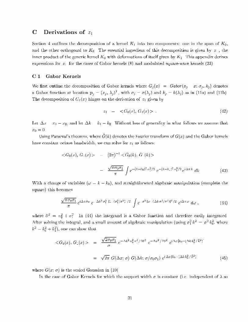
C Derivations of z�

Section � outlines the decomposition of a kernel K� into two components� one in the span of K��

and the other orthogonal to K�� The essential ingredient of this decomposition is given by z� � the

inner product of the generic kernel K� with deformations of itself given by K�� This appendix derives

expressions for z� for the cases of Gabor kernels ��� and modulated square�wave kernels �����

C�� Gabor Kernels

We �rst outline the decomposition of Gabor kernels where Gj�x� � Gabor�xj � x� j� kj� denotes

a Gabor function at location pj � �xj � �j�T � with j � ��j� and kj � k��j� as in �a� and �b��

The decomposition of G��x� hinges on the derivation of z� given by

z� � �G��x�� G��x�� � ����

Let �x � x� � x�� and let �k � k� � k�� Without loss of generality in what follows we assume that

x� � ��

Using Parseval�s theorem� where �G�k� denotes the Fourier transform of G�x� and the Gabor kernels

have constant octave bandwidth� we can solve for z� as follows�

�G��x�� G��x�� � ������� �G��k�� �G��k��

�

p����

Ze��k�k��

� ����� e��k�k��

� ����� ei�x k dk ����

With a change of variables �� � k � k��� and straightforward algebraic manipulation �complete the

square� this becomes

p����

ei�x k� e��k� ��������

������� ��

Ze���� ����k ��

�������� �� ei�x� d� � ����

where �� � �� � �� � In ���� the integrand is a Gabor function and therefore easily integrated�

After solving the integral� and a small amount of algebraic manipulation �using ���k� � �� k�� � where

�k� � k�� � k���� one can show that

�G��x�� G��x�� �

p����

e��k� ������� ���� e��x� � ���� ei�x k���k k�

�� �k���

�p�� G��x� �� G��k� ����� e

i�x k���k k��� �k��� ���

where G�x� � is the scaled Gaussian in ����

In the case of Gabor Kernels for which the support width is constant �i�e� independent of � so

�

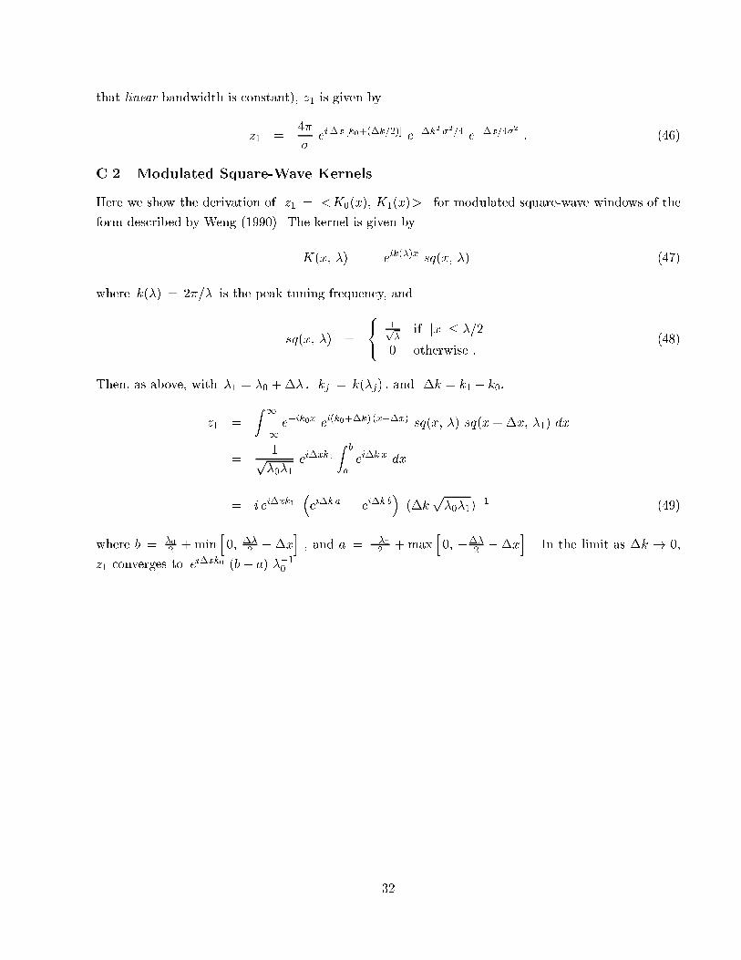
that linear bandwidth is constant�� z� is given by

z� ���

ei�x k���k���� e��k� ���� e��x���� � ����

C�� Modulated Square�Wave Kernels

Here we show the derivation of z� � �K��x�� K��x�� for modulated square�wave windows of the

form described by Weng ������ The kernel is given by

K�x� �� � eik���x sq�x� �� ����

where k��� � ���� is the peak tuning frequency� and

sq�x� �� �

���

�p�

if jxj � ���

� otherwise �����

Then� as above� with �� � �� ��� � kj � k��j� � and �k � k� � k��

z� �

Z �

��e�ik�x ei�k��k� �x�x� sq�x� �� sq�x��x� ��� dx

�p����

ei�xk�

Z b

aei�k x dx

� i ei�xk��ei�k a � ei�k b

���k

p�����

�� ����

where b � ��� � min

h�� ��

� ��xi� and a � ���

� � maxh�� ���

� ��xi� In the limit as �k � ��

z� converges to ei�xk� �b� a� ���� �

��