ST2008S Lecture-03-Quick Review of Probability

Quick Review of Probability

Berlin ChenDepartment of Computer Science & Information Engineering

National Taiwan Normal University

References:1. W. Navidi. Statistics for Engineering and Scientists. Chapter 2 & Teaching Material2. D. P. Bertsekas, J. N. Tsitsiklis. Introduction to Probability.

Statistics-Berlin Chen 2

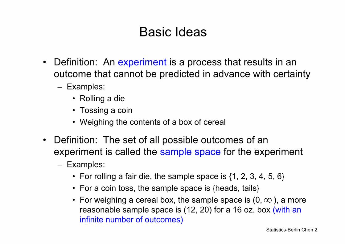
Basic Ideas

• Definition: An experiment is a process that results in an outcome that cannot be predicted in advance with certainty– Examples:

• Rolling a die• Tossing a coin• Weighing the contents of a box of cereal

• Definition: The set of all possible outcomes of an experiment is called the sample space for the experiment– Examples:

• For rolling a fair die, the sample space is {1, 2, 3, 4, 5, 6}• For a coin toss, the sample space is {heads, tails}• For weighing a cereal box, the sample space is (0, ), a more

reasonable sample space is (12, 20) for a 16 oz. box (with an infinite number of outcomes)

∞


More Terminology

Definition: A subset of a sample space is called an event– The empty set Ø is an event– The entire sample space is also an event

• A given event is said to have occurred if the outcome of the experiment is one of the outcomes in the event. For example, if a die comes up 2, the events {2, 4, 6} and {1, 2, 3} have both occurred, along with every other event that contains the outcome “2”


Combining Events

• The union of two events A and B, denoted A ∪ B, is the set of outcomes that belong either to A, to B, or to both

– In words, A ∪ B means “A or B”. So the event “A or B” occurs whenever either A or B (or both) occurs

• Example: Let A = {1, 2, 3} and B = {2, 3, 4} Then A ∪ B = {1, 2, 3, 4}


Intersections

• The intersection of two events A and B, denoted by A ∩ B, is the set of outcomes that belong to A and to B

– In words, A ∩ B means “A and B”. Thus the event “A and B”occurs whenever both A and B occur

• Example: Let A = {1, 2, 3} and B = {2, 3, 4}Then A ∩ B = {2, 3}


Complements

• The complement of an event A, denoted Ac, is the set of outcomes that do not belong to A

– In words, Ac means “not A”. Thus the event “not A” occurs whenever A does not occur

• Example: Consider rolling a fair sided die. Let A be the event: “rolling a six” = {6}. Then Ac = “not rolling a six” = {1, 2, 3, 4, 5}


Mutually Exclusive Events

• Definition: The events A and B are said to be mutually exclusive if they have no outcomes in common

– More generally, a collection of events is said to be mutually exclusive if no two of them have any outcomes in common

• Sometimes mutually exclusive events are referred to as disjoint events

1 2, ,..., nA A A


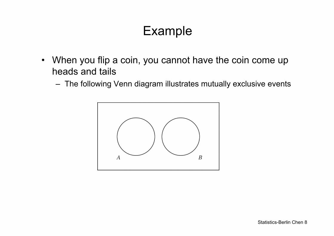
Example

• When you flip a coin, you cannot have the coin come up heads and tails – The following Venn diagram illustrates mutually exclusive events


Probabilities

• Definition: Each event in the sample space has a probability of occurring. Intuitively, the probability is a quantitative measure of how likely the event is to occur

• Given any experiment and any event A:– The expression P(A) denotes the probability that the event A

occurs– P(A) is the proportion of times that the event A would occur in

the long run, if the experiment were to be repeated over and over again


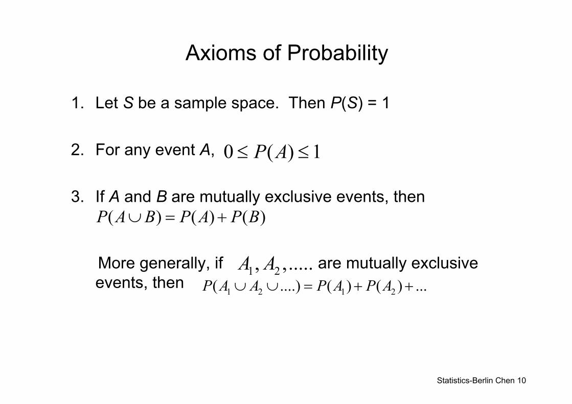
Axioms of Probability

1. Let S be a sample space. Then P(S) = 1

2. For any event A,

3. If A and B are mutually exclusive events, then

More generally, if are mutually exclusive events, then

0 ( ) 1P A≤ ≤

( ) ( ) ( )P A B P A P B∪ = +

1 2, ,.....A A1 2 1 2( ....) ( ) ( ) ...P A A P A P A∪ ∪ = + +


A Few Useful Things

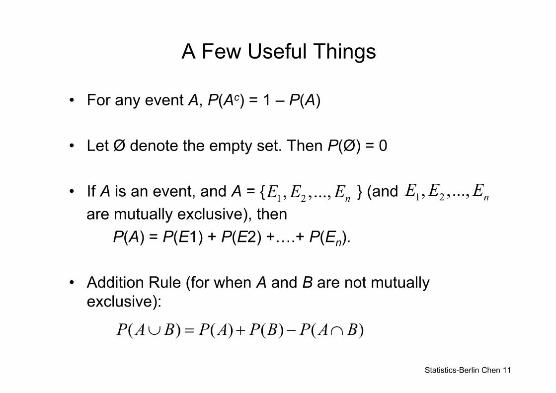
• For any event A, P(Ac) = 1 – P(A)

• Let Ø denote the empty set. Then P(Ø) = 0

• If A is an event, and A = { } (and are mutually exclusive), then

P(A) = P(E1) + P(E2) +….+ P(En).

• Addition Rule (for when A and B are not mutually exclusive):

1 2, ,..., nE E E 1 2, ,..., nE E E

( ) ( ) ( ) ( )P A B P A P B P A B∪ = + − ∩


Conditional Probability and Independence

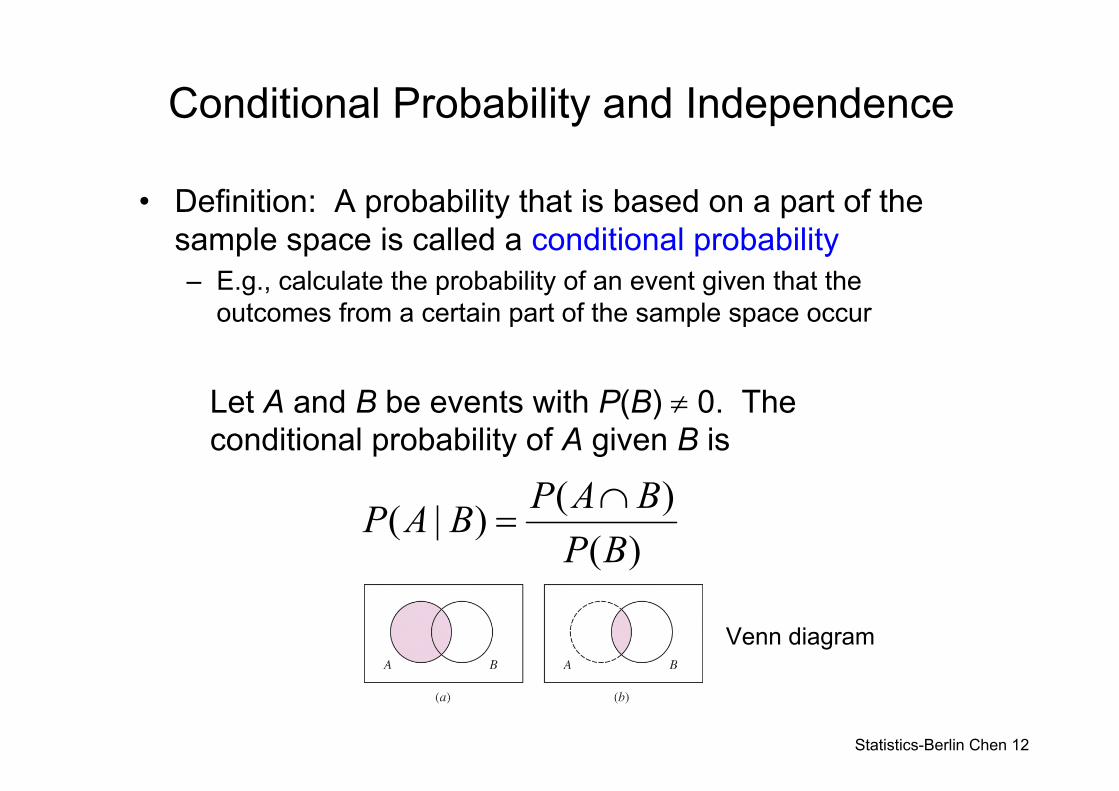
• Definition: A probability that is based on a part of the sample space is called a conditional probability– E.g., calculate the probability of an event given that the

outcomes from a certain part of the sample space occur

Let A and B be events with P(B) ≠ 0. The conditional probability of A given B is

( )( | )( )

P A BP A BP B∩

=

Venn diagram


More Definitions

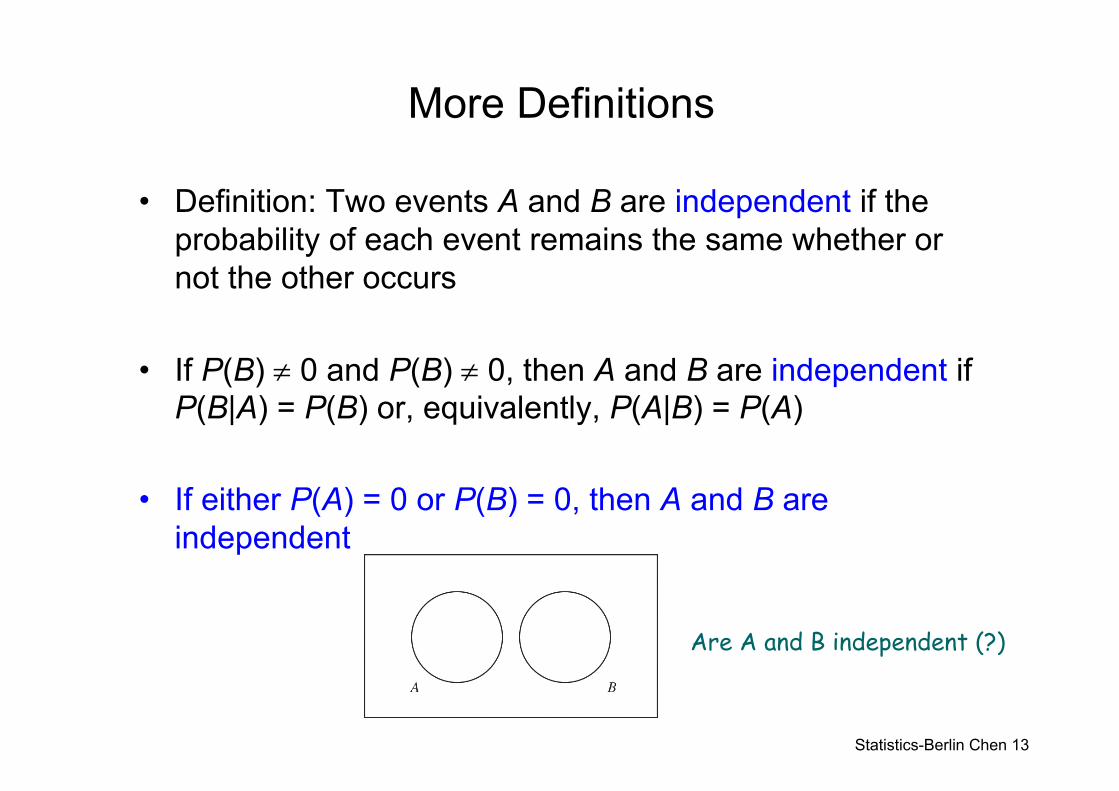
• Definition: Two events A and B are independent if the probability of each event remains the same whether or not the other occurs

• If P(B) ≠ 0 and P(B) ≠ 0, then A and B are independent if P(B|A) = P(B) or, equivalently, P(A|B) = P(A)

• If either P(A) = 0 or P(B) = 0, then A and B are independent

Are A and B independent (?)


The Multiplication (Chain) Rule

• If A and B are two events and P(B) ≠ 0, then P(A ∩ B) = P(B)P(A|B)

• If A and B are two events and P(A) ≠ 0, then P(A ∩ B) = P(A)P(B|A)

• If P(A) ≠ 0, and P(B) ≠ 0, then both of the above hold

• If A and B are two independent events, then P(A ∩ B) = P(A)P(B)

• This result can be extended to more than two events


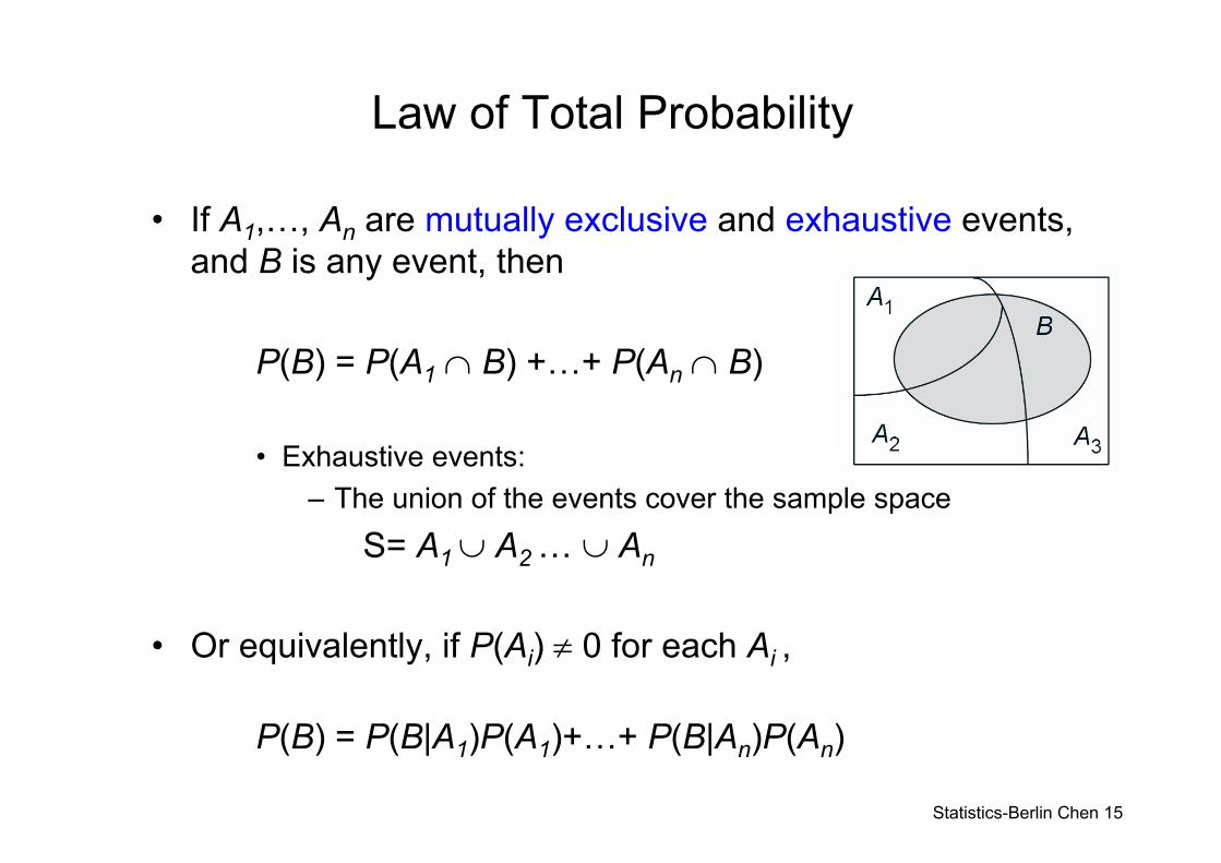
Law of Total Probability

• If A1,…, An are mutually exclusive and exhaustive events, and B is any event, then

P(B) = P(A1 ∩ B) +…+ P(An ∩ B)

• Exhaustive events:– The union of the events cover the sample space

S= A1 ∪ A2 … ∪ An

• Or equivalently, if P(Ai) ≠ 0 for each Ai ,

P(B) = P(B|A1)P(A1)+…+ P(B|An)P(An)


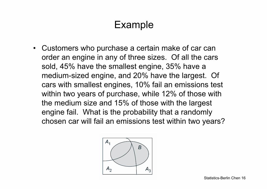
Example

• Customers who purchase a certain make of car can order an engine in any of three sizes. Of all the cars sold, 45% have the smallest engine, 35% have a medium-sized engine, and 20% have the largest. Of cars with smallest engines, 10% fail an emissions test within two years of purchase, while 12% of those with the medium size and 15% of those with the largest engine fail. What is the probability that a randomly chosen car will fail an emissions test within two years?


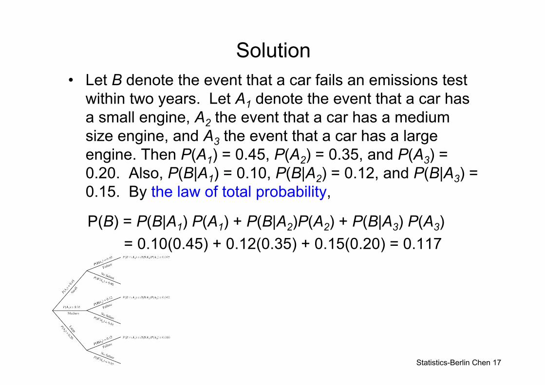
Solution• Let B denote the event that a car fails an emissions test

within two years. Let A1 denote the event that a car has a small engine, A2 the event that a car has a medium size engine, and A3 the event that a car has a large engine. Then P(A1) = 0.45, P(A2) = 0.35, and P(A3) = 0.20. Also, P(B|A1) = 0.10, P(B|A2) = 0.12, and P(B|A3) = 0.15. By the law of total probability,

P(B) = P(B|A1) P(A1) + P(B|A2)P(A2) + P(B|A3) P(A3) = 0.10(0.45) + 0.12(0.35) + 0.15(0.20) = 0.117


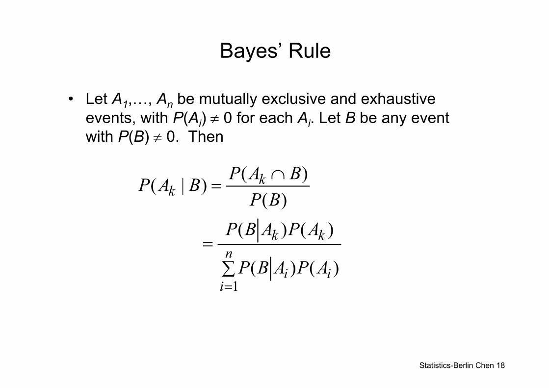
Bayes’ Rule

• Let A1,…, An be mutually exclusive and exhaustive events, with P(Ai) ≠ 0 for each Ai. Let B be any event with P(B) ≠ 0. Then

∑=

∩=

=

n

iii

kk

kk

APABP

APABPBPBAPBAP

1)()(

)()(

)()()|(


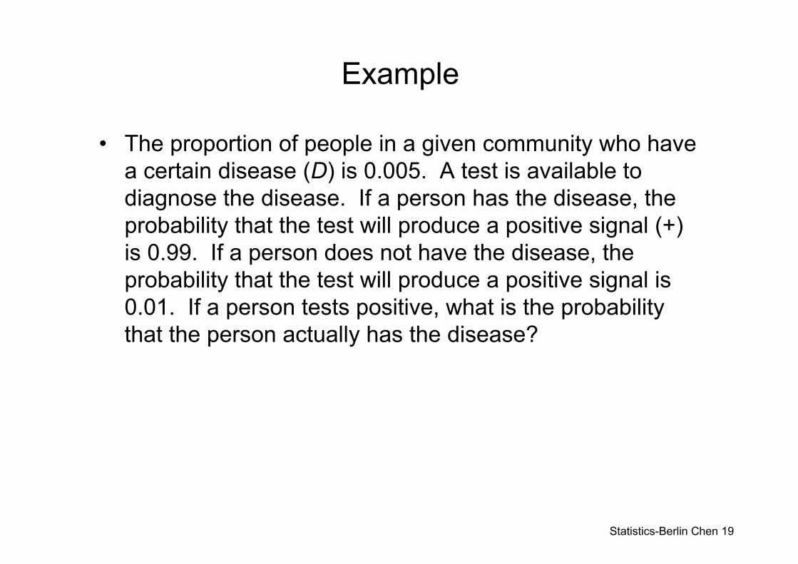
Example

• The proportion of people in a given community who have a certain disease (D) is 0.005. A test is available to diagnose the disease. If a person has the disease, the probability that the test will produce a positive signal (+) is 0.99. If a person does not have the disease, the probability that the test will produce a positive signal is 0.01. If a person tests positive, what is the probability that the person actually has the disease?


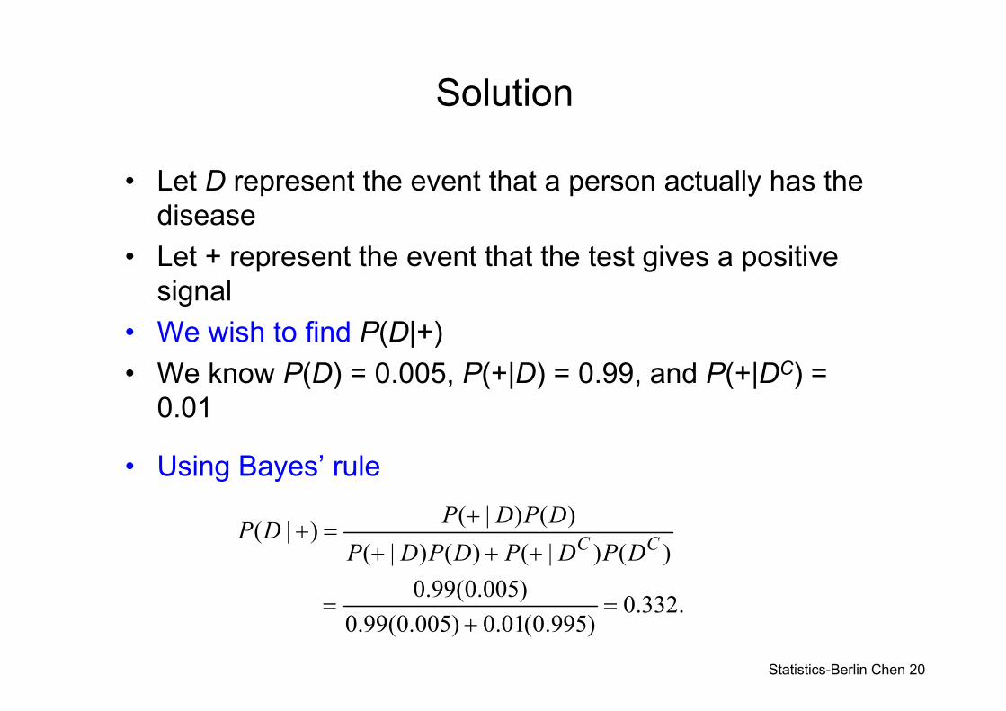
Solution

• Let D represent the event that a person actually has the disease

• Let + represent the event that the test gives a positive signal

• We wish to find P(D|+)• We know P(D) = 0.005, P(+|D) = 0.99, and P(+|DC) =

0.01

• Using Bayes’ rule

.332.0)995.0(01.0)005.0(99.0

)005.0(99.0

)()|()()|()()|()|(

=+

=

+++

+=+ CC DPDPDPDP

DPDPDP


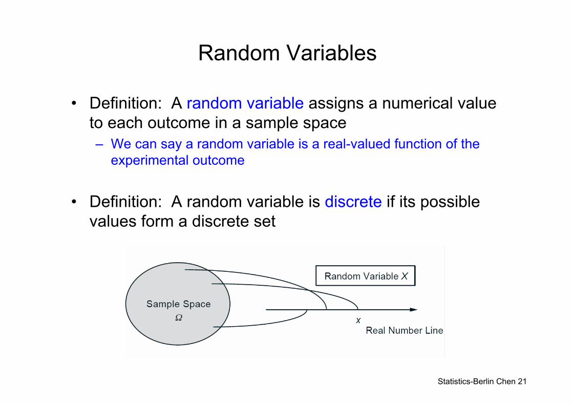
Random Variables

• Definition: A random variable assigns a numerical value to each outcome in a sample space– We can say a random variable is a real-valued function of the

experimental outcome

• Definition: A random variable is discrete if its possible values form a discrete set


Example

• The number of flaws in a 1-inch length of copper wire manufactured by a certain process varies from wire to wire. Overall, 48% of the wires produced have no flaws, 39% have one flaw, 12% have two flaws, and 1% have three flaws. Let X be the number of flaws in a randomly selected piece of wire

• Then,– P(X = 0) = 0.48, P(X = 1) = 0.39, P(X = 2) = 0.12,

and P(X = 3) = 0.01– The list of possible values 0, 1, 2, and 3, along with the

probabilities of each, provide a complete description of the population from which X was drawn


Probability Mass Function

• The description of the possible values of X and the probabilities of each has a name: – The probability mass function

• Definition: The probability mass function (denoted as pmf) of a discrete random variable X is the function p(x) = P(X = x). The probability mass function is sometimes called the probability distribution


Cumulative Distribution Function

• The probability mass function specifies the probability that a random variable is equal to a given value

• A function called the cumulative distribution function(cdf) specifies the probability that a random variable is less than or equal to a given value

• The cumulative distribution function of the random variable X is the function F(x) = P(X ≤ x)


Example

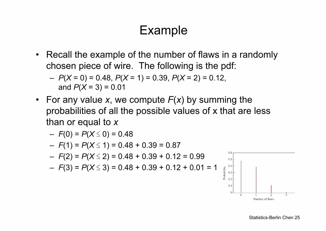
• Recall the example of the number of flaws in a randomly chosen piece of wire. The following is the pdf:– P(X = 0) = 0.48, P(X = 1) = 0.39, P(X = 2) = 0.12,

and P(X = 3) = 0.01

• For any value x, we compute F(x) by summing the probabilities of all the possible values of x that are less than or equal to x– F(0) = P(X ≤ 0) = 0.48– F(1) = P(X ≤ 1) = 0.48 + 0.39 = 0.87– F(2) = P(X ≤ 2) = 0.48 + 0.39 + 0.12 = 0.99– F(3) = P(X ≤ 3) = 0.48 + 0.39 + 0.12 + 0.01 = 1


More on Discrete Random Variables

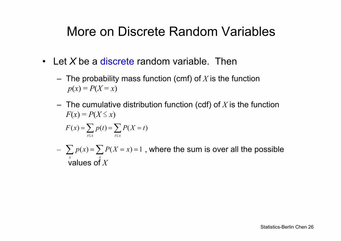
• Let X be a discrete random variable. Then

– The probability mass function (cmf) of X is the functionp(x) = P(X = x)

– The cumulative distribution function (cdf) of X is the function F(x) = P(X ≤ x)

– , where the sum is over all the possiblevalues of X

( ) ( ) ( )t x t x

F x p t P X t≤ ≤

= = =∑ ∑

( ) ( ) 1x xp x P X x= = =∑ ∑


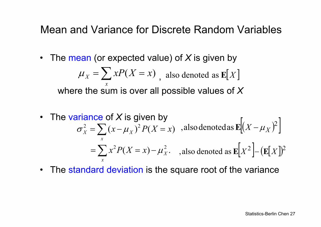
Mean and Variance for Discrete Random Variables

• The mean (or expected value) of X is given by

,where the sum is over all possible values of X

• The variance of X is given by

• The standard deviation is the square root of the variance

( )XxxP X xμ = =∑

2 2

2 2

( ) ( )

( ) .

X Xx

Xx

x P X x

x P X x

σ μ

μ

= − =

= = −

∑

∑

[ ]XE as denoted also

( )[ ]2 as denoted also, XX μ−E

[ ] [ ]( )22 as denoted also, XX EE −


The Probability Histogram

• When the possible values of a discrete random variable are evenly spaced, the probability mass function can be represented by a histogram, with rectangles centered at the possible values of the random variable

• The area of the rectangle centered at a value x is equal to P(X = x)

• Such a histogram is called a probability histogram, because the areas represent probabilities


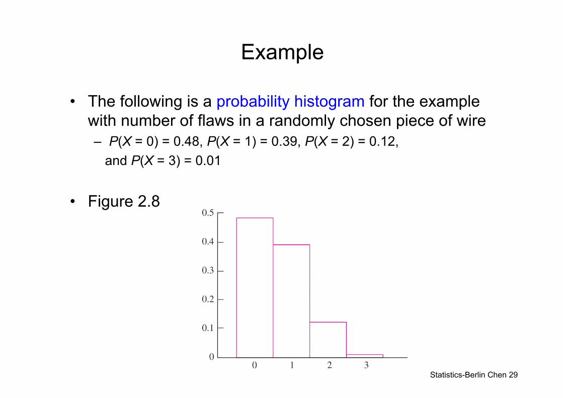
Example

• The following is a probability histogram for the example with number of flaws in a randomly chosen piece of wire– P(X = 0) = 0.48, P(X = 1) = 0.39, P(X = 2) = 0.12,

and P(X = 3) = 0.01

• Figure 2.8


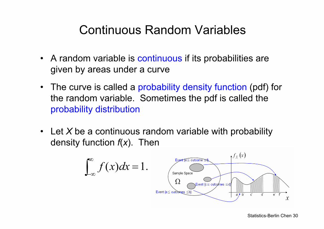
Continuous Random Variables

• A random variable is continuous if its probabilities are given by areas under a curve

• The curve is called a probability density function (pdf) for the random variable. Sometimes the pdf is called the probability distribution

• Let X be a continuous random variable with probability density function f(x). Then

( ) 1.f x dx∞

−∞=∫


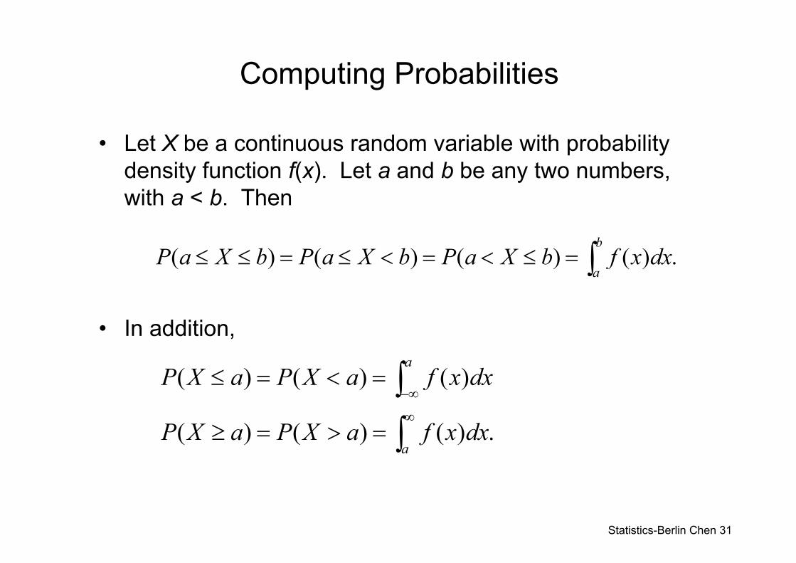
Computing Probabilities

• Let X be a continuous random variable with probability density function f(x). Let a and b be any two numbers, with a < b. Then

• In addition,

( ) ( ) ( ) ( ) .b

aP a X b P a X b P a X b f x dx≤ ≤ = ≤ < = < ≤ = ∫

( ) ( ) ( )

( ) ( ) ( ) .

a

a

P X a P X a f x dx

P X a P X a f x dx

−∞

∞

≤ = < =

≥ = > =

∫∫


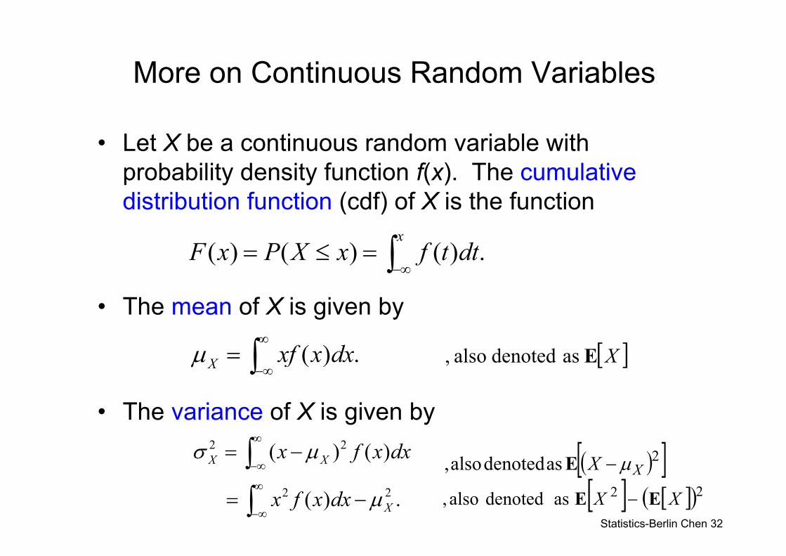
More on Continuous Random Variables

• Let X be a continuous random variable with probability density function f(x). The cumulative distribution function (cdf) of X is the function

• The mean of X is given by

• The variance of X is given by

( ) ( ) ( ) .x

F x P X x f t dt−∞

= ≤ = ∫

( ) .X xf x dxμ∞

−∞= ∫

2 2

2 2

( ) ( )

( ) .

X X

X

x f x dx

x f x dx

σ μ

μ

∞

−∞

∞

−∞

= −

= −

∫∫

[ ]XE as denoted also ,

( )[ ]2 as denoted also, XX μ−E

[ ] [ ]( )22 as denoted also, XX EE −


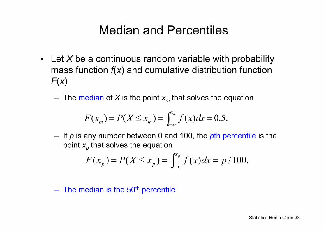
Median and Percentiles

• Let X be a continuous random variable with probability mass function f(x) and cumulative distribution function F(x)

– The median of X is the point xm that solves the equation

– If p is any number between 0 and 100, the pth percentile is the point xp that solves the equation

– The median is the 50th percentile

( ) ( ) ( ) 0.5.mx

m mF x P X x f x dx−∞

= ≤ = =∫

( ) ( ) ( ) /100.px

p pF x P X x f x dx p−∞

= ≤ = =∫


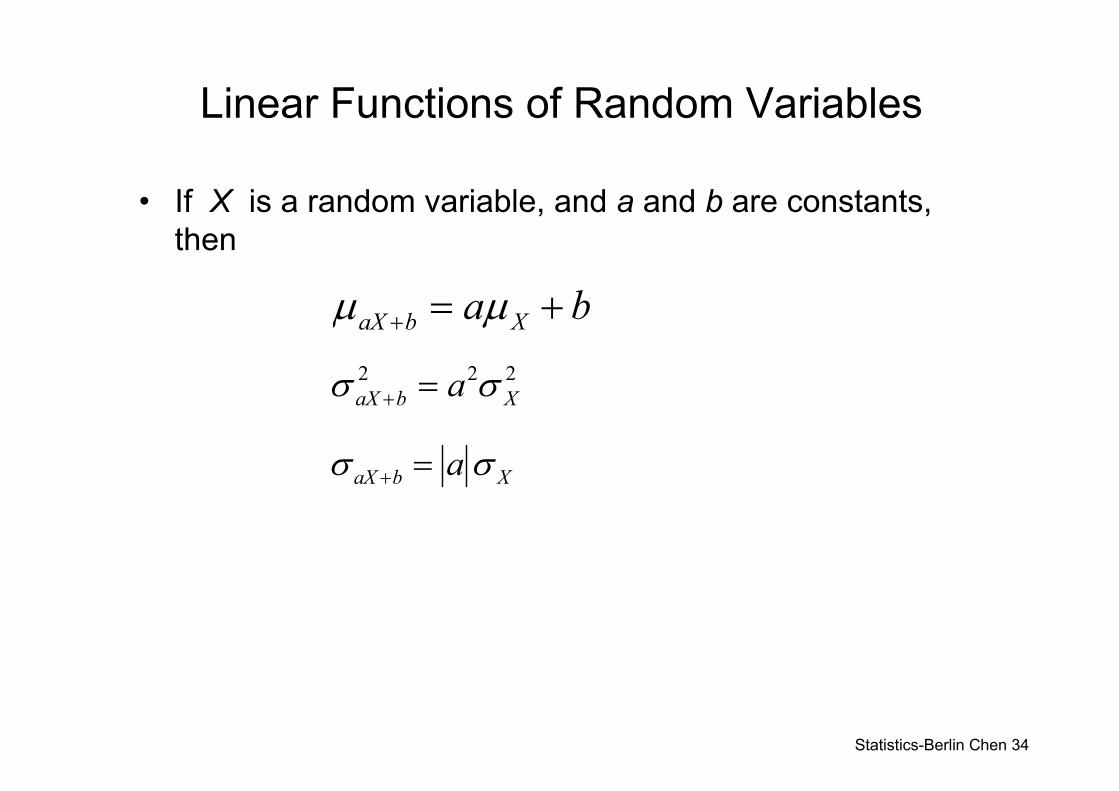
Linear Functions of Random Variables

• If X is a random variable, and a and b are constants, then

aX b Xa bμ μ+ = +2 2 2aX b Xaσ σ+ =

aX b Xaσ σ+ =


More Linear Functions

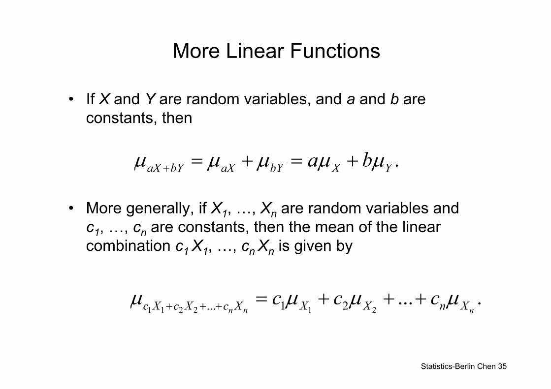
• If X and Y are random variables, and a and b are constants, then

• More generally, if X1, …, Xn are random variables and c1, …, cn are constants, then the mean of the linear combination c1 X1, …, cn Xn is given by

.aX bY aX bY X Ya bμ μ μ μ μ+ = + = +

1 1 2 2 1 2... 1 2 ... .n n nc X c X c X X X n Xc c cμ μ μ μ+ + + = + + +


Two Independent Random Variables

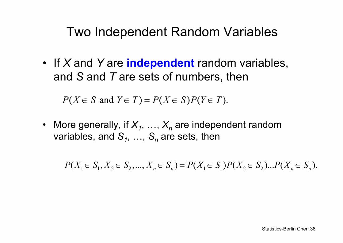
• If X and Y are independent random variables, and S and T are sets of numbers, then

• More generally, if X1, …, Xn are independent random variables, and S1, …, Sn are sets, then

( and ) ( ) ( ).P X S Y T P X S P Y T∈ ∈ = ∈ ∈

1 1 2 2 1 1 2 2( , ,..., ) ( ) ( )... ( ).n n n nP X S X S X S P X S P X S P X S∈ ∈ ∈ = ∈ ∈ ∈


Variance Properties

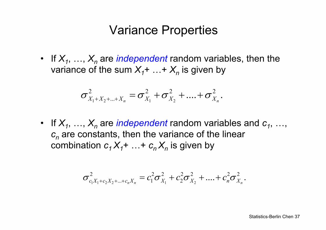
• If X1, …, Xn are independent random variables, then the variance of the sum X1+ …+ Xn is given by

• If X1, …, Xn are independent random variables and c1, …, cn are constants, then the variance of the linear combination c1 X1+ …+ cn Xn is given by

1 2 1 2

2 2 2 2... .... .

n nX X X X X Xσ σ σ σ+ + + = + + +

1 1 2 2 1 2

2 2 2 2 2 2 2... 1 2 .... .

n n nc X c X c X X X n Xc c cσ σ σ σ+ + + = + + +


More Variance Properties

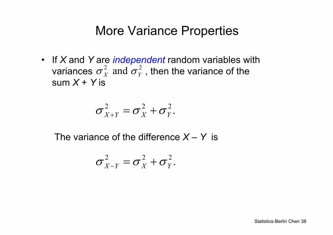
• If X and Y are independent random variables with variances , then the variance of the sum X + Y is

The variance of the difference X – Y is

2 2and X Yσ σ

2 2 2.X Y X Yσ σ σ+ = +

2 2 2.X Y X Yσ σ σ− = +


Independence and Simple Random Samples

• Definition: If X1, …, Xn is a simple random sample, then X1, …, Xn may be treated as independent random variables, all from the same population

– Phrased another way, X1, …, Xn are independent, and identically distributed (i.i.d.)


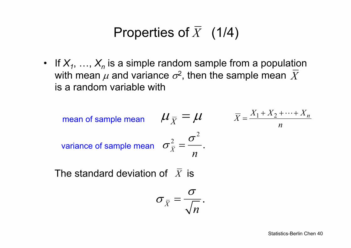
Properties of (1/4)

• If X1, …, Xn is a simple random sample from a population with mean μ and variance σ2, then the sample mean is a random variable with

The standard deviation of is

X

X

Xμ μ=2

2 .X nσσ =

X

.X nσσ =

mean of sample mean

variance of sample mean

nXXXX n+++

=L21


Properties of (2/4) X

39....354037sample mean

)2.40(2 == xX38.5....423841 sample mean

40.2....423837.5 sample mean

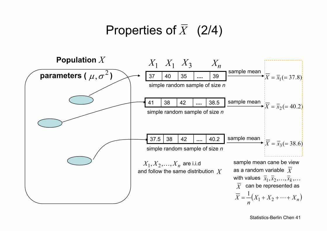
Population

parameters ( ) 2 ,σμ

X1X 1X 3X nX

simple random sample of size n

sample mean cane be view as a random variable with values

can be represented as

XKK ,,,, 21 kxxx

X

( )nXXXn

X +++= L211

nXXX ,,, 21 K are i.i.dand follow the same distribution X



)8.37(1 == xX

)6.38(3 == xX


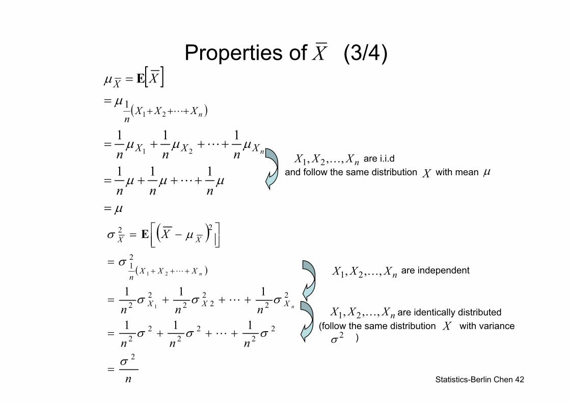
Properties of (3/4) X[ ]

( )

μ

μμμ

μμμ

μμ

=

+++=

+++=

=

=

+++

nnn

nnn

X

n

n

XXX

XXXn

X

111

11121

211

L

L

L

E

nXXX ,,, 21 K are i.i.dand follow the same distribution with mean

X

μ

( )

( )

n

nnn

nnn

X

n

n

XXX

XXXn

XX

2

22

22

22

22

222

22

21

22

111

1111

21

σ

σσσ

σσσ

σ

μσ

=

+++=

+++=

=

⎥⎦⎤

⎢⎣⎡ −=

+++

L

L

L

E

nXXX ,,, 21 K

are identically distributed(follow the same distribution with variance

)

nXXX ,,, 21 K

2σ

X

are independent


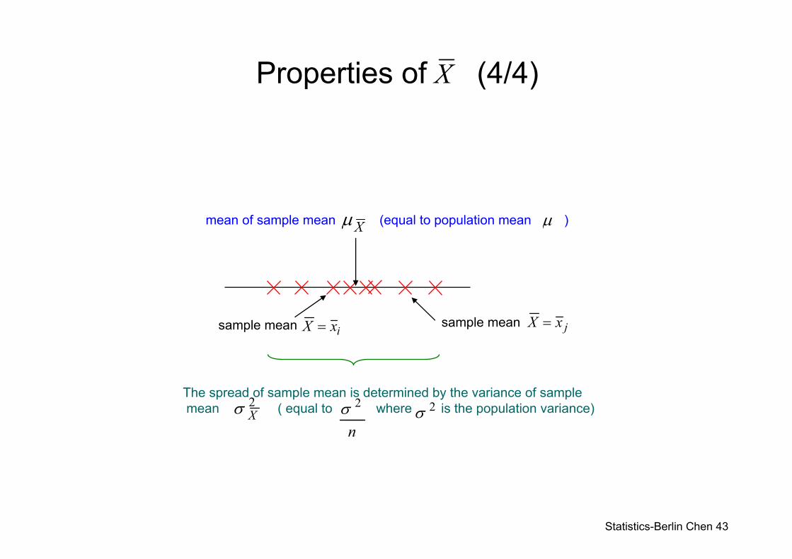
Properties of (4/4)

sample mean sample mean ixX =

mean of sample mean (equal to population mean )Xμ μ

X

The spread of sample mean is determined by the variance of sample mean ( equal to where is the population variance)2

Xσn

2σ 2σ

jxX =


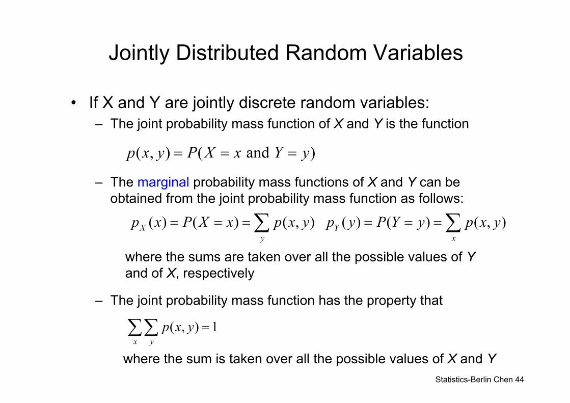
Jointly Distributed Random Variables

• If X and Y are jointly discrete random variables:– The joint probability mass function of X and Y is the function

– The marginal probability mass functions of X and Y can be obtained from the joint probability mass function as follows:

where the sums are taken over all the possible values of Yand of X, respectively

– The joint probability mass function has the property that

where the sum is taken over all the possible values of X and Y

( , ) ( and )p x y P X x Y y= = =

( ) ( ) ( , ) ( ) ( ) ( , ) X Yy x

p x P X x p x y p y P Y y p x y= = = = = =∑ ∑

( , ) 1x y

p x y =∑∑


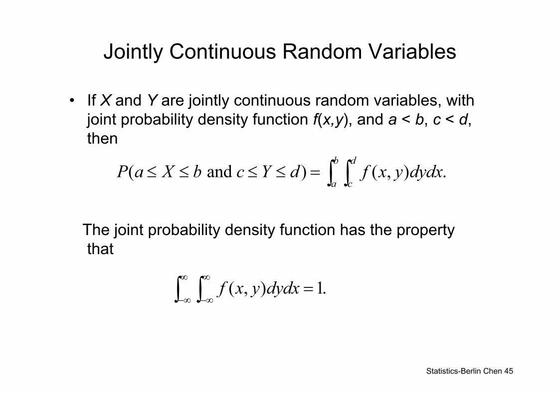
Jointly Continuous Random Variables

• If X and Y are jointly continuous random variables, with joint probability density function f(x,y), and a < b, c < d, then

The joint probability density function has the property that

( and ) ( , ) .b d

a cP a X b c Y d f x y dydx≤ ≤ ≤ ≤ = ∫ ∫

( , ) 1.f x y dydx∞ ∞

−∞ −∞=∫ ∫


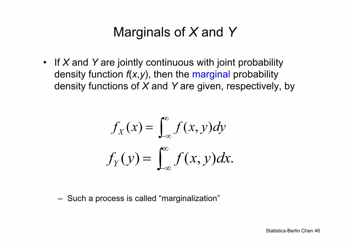
Marginals of X and Y

• If X and Y are jointly continuous with joint probability density function f(x,y), then the marginal probability density functions of X and Y are given, respectively, by

– Such a process is called “marginalization”

( ) ( , )Xf x f x y dy∞

−∞= ∫

( ) ( , ) .Yf y f x y dx∞

−∞= ∫


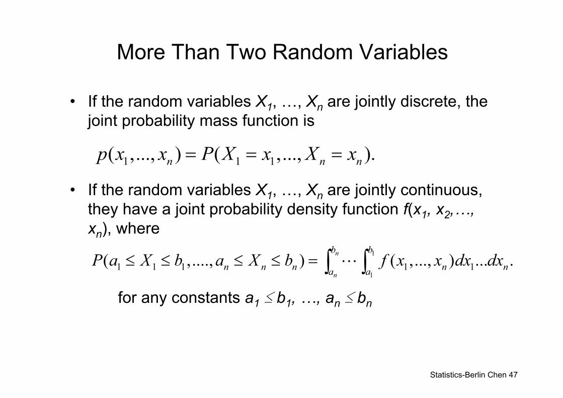
More Than Two Random Variables

• If the random variables X1, …, Xn are jointly discrete, the joint probability mass function is

• If the random variables X1, …, Xn are jointly continuous, they have a joint probability density function f(x1, x2,…, xn), where

for any constants a1 ≤ b1, …, an ≤ bn

1 1 1( ,..., ) ( ,..., ).n n np x x P X x X x= = =

1

11 1 1 1 1( ,...., ) ( ,..., ) ... .n

n

b b

n n n n na aP a X b a X b f x x dx dx≤ ≤ ≤ ≤ = ∫ ∫L


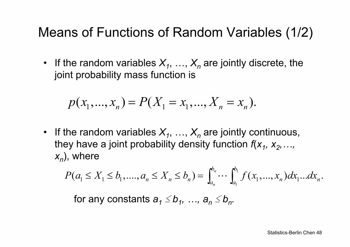
Means of Functions of Random Variables (1/2)

• If the random variables X1, …, Xn are jointly discrete, the joint probability mass function is

• If the random variables X1, …, Xn are jointly continuous, they have a joint probability density function f(x1, x2,…, xn), where

for any constants a1 ≤ b1, …, an ≤ bn.

1 1 1( ,..., ) ( ,..., ).n n np x x P X x X x= = =

1

11 1 1 1 1( ,...., ) ( ,..., ) ... .n

n

b b

n n n n na aP a X b a X b f x x dx dx≤ ≤ ≤ ≤ = ∫ ∫L


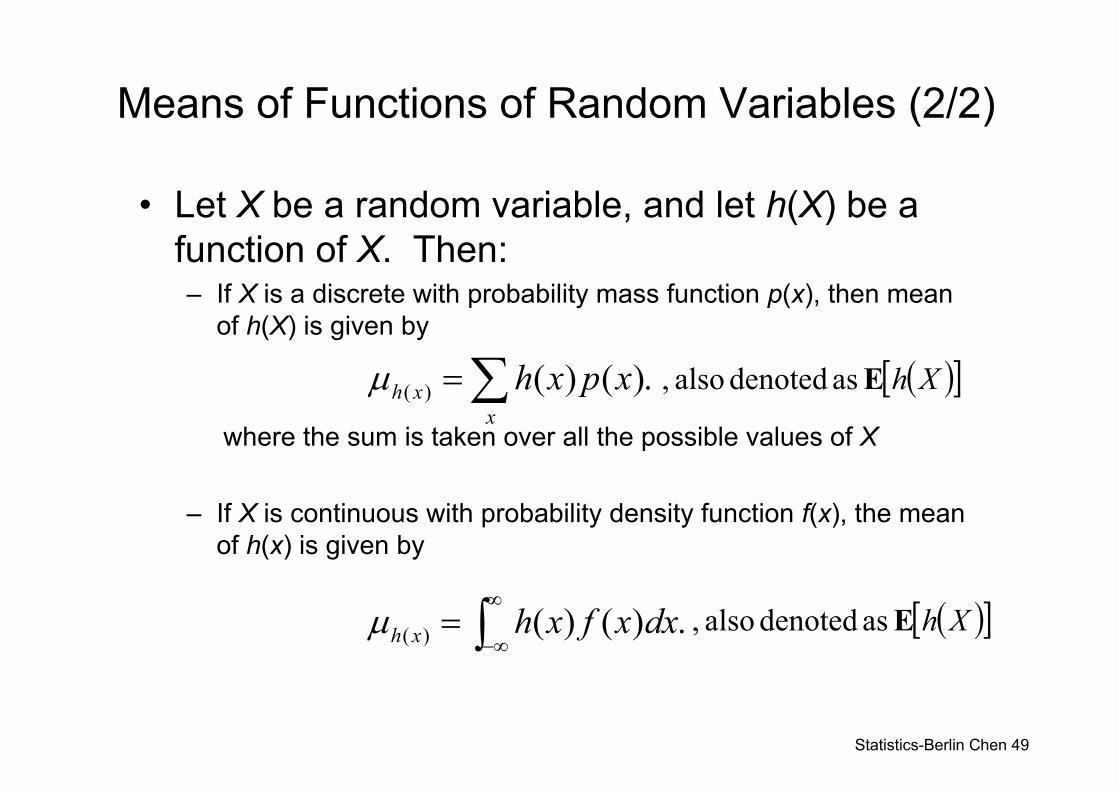
Means of Functions of Random Variables (2/2)

• Let X be a random variable, and let h(X) be a function of X. Then:– If X is a discrete with probability mass function p(x), then mean

of h(X) is given by

where the sum is taken over all the possible values of X

– If X is continuous with probability density function f(x), the mean of h(x) is given by

( ) ( ) ( ).h xxh x p xμ =∑

( ) ( ) ( ) .h x h x f x dxμ∞

−∞= ∫

( )[ ]XhE as denoted also ,

( )[ ]XhE as denoted also ,


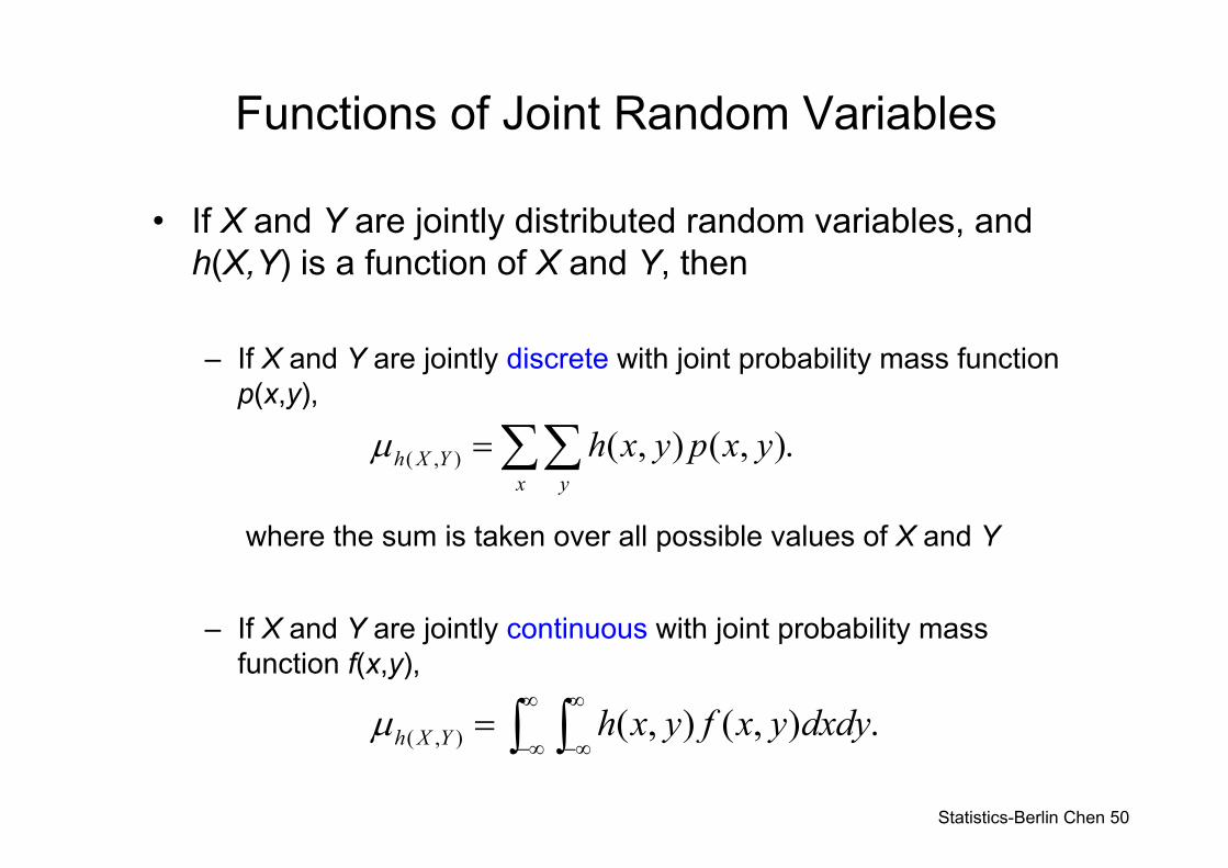
Functions of Joint Random Variables

• If X and Y are jointly distributed random variables, and h(X,Y) is a function of X and Y, then

– If X and Y are jointly discrete with joint probability mass function p(x,y),

where the sum is taken over all possible values of X and Y

– If X and Y are jointly continuous with joint probability mass function f(x,y),

( , ) ( , ) ( , ).h X Yx y

h x y p x yμ =∑∑

( , ) ( , ) ( , ) .h X Y h x y f x y dxdyμ∞ ∞

−∞ −∞= ∫ ∫


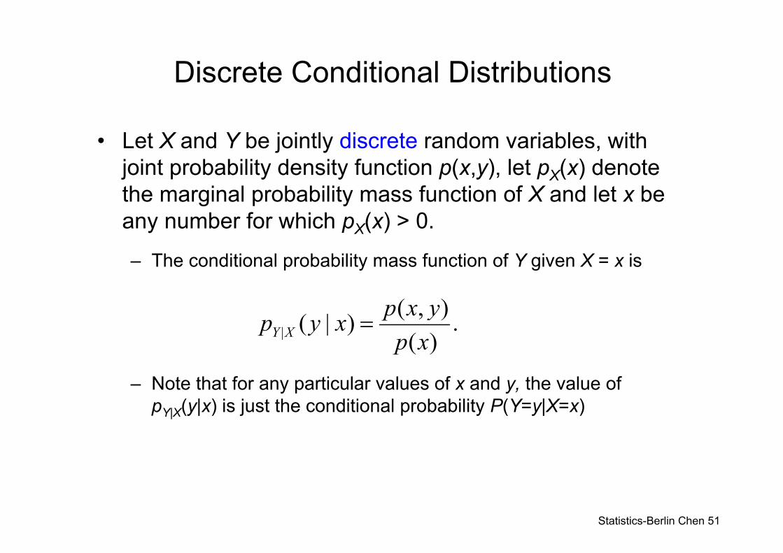
Discrete Conditional Distributions

• Let X and Y be jointly discrete random variables, with joint probability density function p(x,y), let pX(x) denote the marginal probability mass function of X and let x be any number for which pX(x) > 0.

– The conditional probability mass function of Y given X = x is

– Note that for any particular values of x and y, the value of pY|X(y|x) is just the conditional probability P(Y=y|X=x)

|( , )( | ) .( )Y X

p x yp y xp x

=


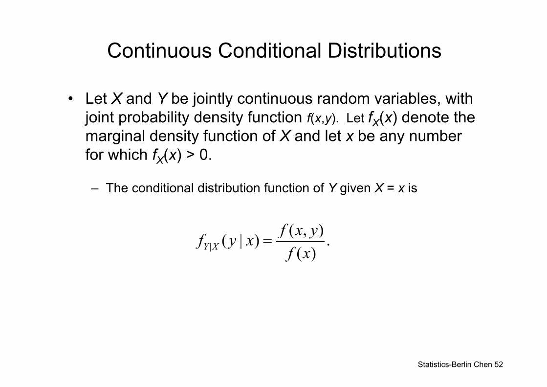
Continuous Conditional Distributions

• Let X and Y be jointly continuous random variables, with joint probability density function f(x,y). Let fX(x) denote the marginal density function of X and let x be any number for which fX(x) > 0.

– The conditional distribution function of Y given X = x is

|( , )( | ) .( )Y X

f x yf y xf x

=


Conditional Expectation

• Expectation is another term for mean

• A conditional expectation is an expectation, or mean, calculated using the conditional probability mass function or conditional probability density function

• The conditional expectation of Y given X = x is denoted by E(Y|X = x) or μY|X


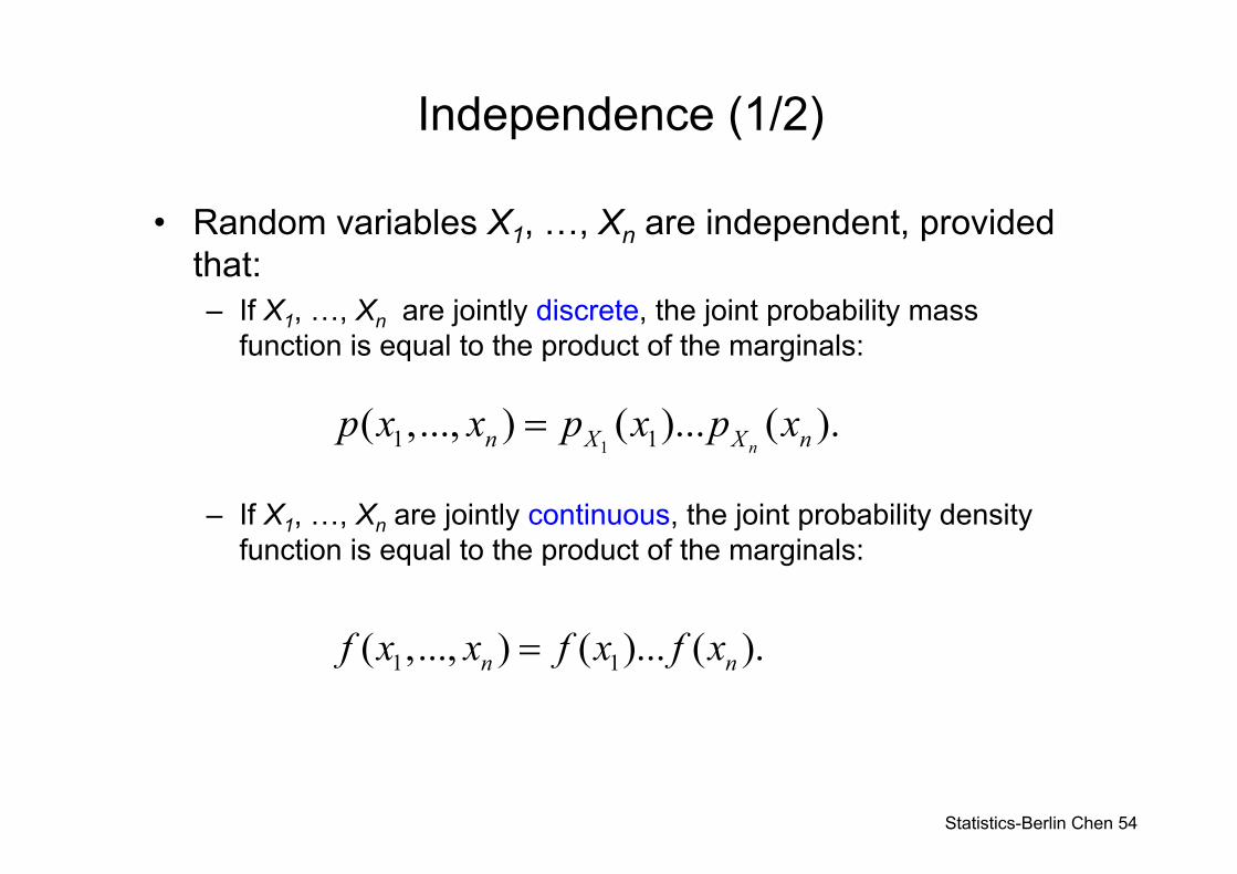
Independence (1/2)

• Random variables X1, …, Xn are independent, provided that: – If X1, …, Xn are jointly discrete, the joint probability mass

function is equal to the product of the marginals:

– If X1, …, Xn are jointly continuous, the joint probability density function is equal to the product of the marginals:

11 1( ,..., ) ( )... ( ).nn X X np x x p x p x=

1 1( ,..., ) ( )... ( ).n nf x x f x f x=


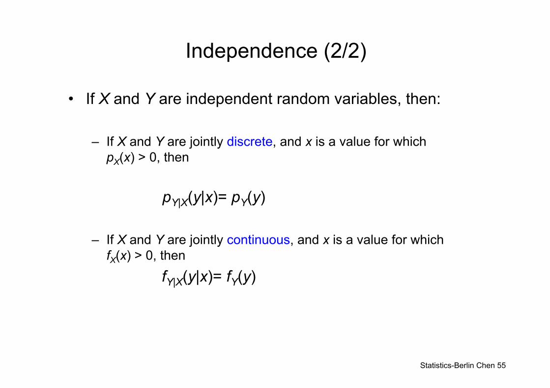
Independence (2/2)

• If X and Y are independent random variables, then:

– If X and Y are jointly discrete, and x is a value for which pX(x) > 0, then

pY|X(y|x)= pY(y)

– If X and Y are jointly continuous, and x is a value for which fX(x) > 0, then

fY|X(y|x)= fY(y)


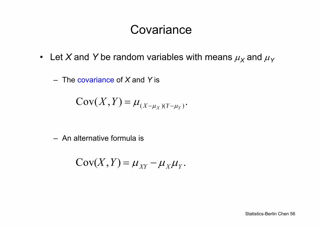
Covariance

• Let X and Y be random variables with means μX and μY

– The covariance of X and Y is

– An alternative formula is

( )( )Cov( , ) .X YX YX Y μ μμ − −=

Cov( , ) .XY X YX Y μ μ μ= −


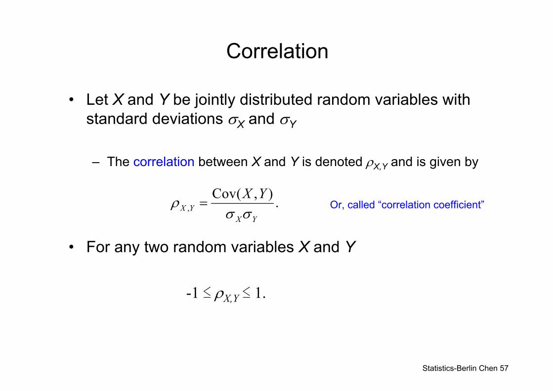
Correlation

• Let X and Y be jointly distributed random variables with standard deviations σX and σY

– The correlation between X and Y is denoted ρX,Y and is given by

• For any two random variables X and Y

-1 ≤ ρX,Y ≤ 1.

,Cov( , ) .X Y

X Y

X Yρσ σ

= Or, called “correlation coefficient”


Covariance, Correlation, and Independence

• If Cov(X,Y) = ρX,Y = 0, then X and Y are said to be uncorrelated

• If X and Y are independent, then X and Y are uncorrelated

• It is mathematically possible for X and Y to be uncorrelated without being independent. This rarely occurs in practice


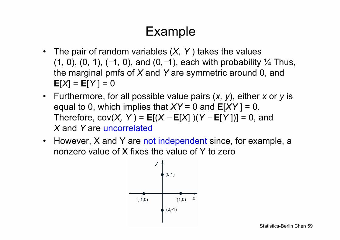
Example• The pair of random variables (X, Y ) takes the values

(1, 0), (0, 1), (−1, 0), and (0,−1), each with probability ¼ Thus, the marginal pmfs of X and Y are symmetric around 0, and E[X] = E[Y ] = 0

• Furthermore, for all possible value pairs (x, y), either x or y is equal to 0, which implies that XY = 0 and E[XY ] = 0. Therefore, cov(X, Y ) = E[(X − E[X] )(Y − E[Y ])] = 0, and X and Y are uncorrelated

• However, X and Y are not independent since, for example, a nonzero value of X fixes the value of Y to zero


Variance of a Linear Combination of Random Variables (1/2)

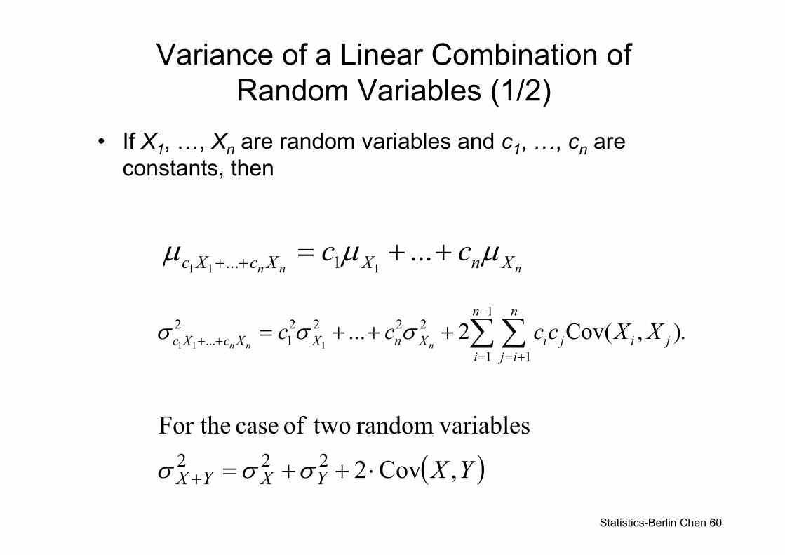
• If X1, …, Xn are random variables and c1, …, cn are constants, then

1 1 1... 1 ...n n nc X c X X n Xc cμ μ μ+ + = + +

1 1 1

12 2 2 2 2

... 11 1

... 2 Cov( , ).n n n

n n

c X c X X n X i j i ji j i

c c c c X Xσ σ σ−

+ += = +

= + + + ∑ ∑

( )YXYXYX ,Cov2

variablesrandom twoof case For the222 ⋅++=+ σσσ


Variance of a Linear Combination of Random Variables (2/2)

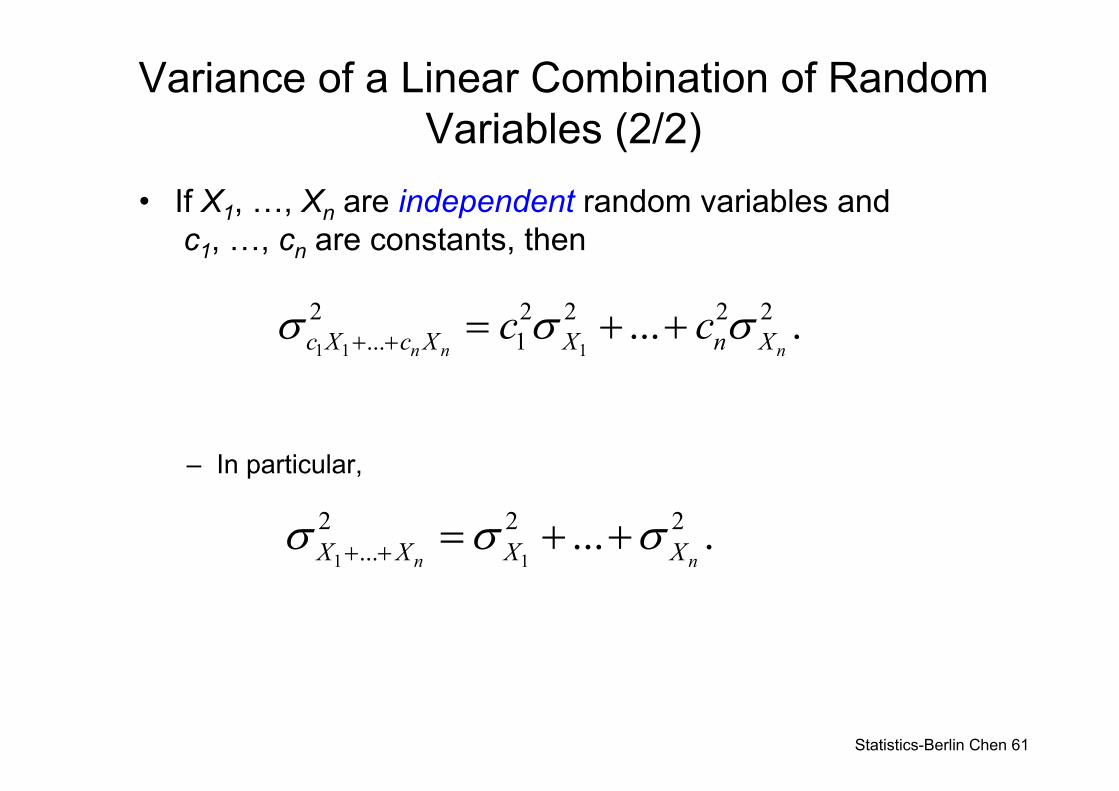
• If X1, …, Xn are independent random variables andc1, …, cn are constants, then

– In particular,

1 1 1

2 2 2 2 2... 1 ... .

n n nc X c X X n Xc cσ σ σ+ + = + +

1 1

2 2 2... ... .

n nX X X Xσ σ σ+ + = + +


Summary (1/2)

• Probability and rules

• Counting techniques

• Conditional probability

• Independence

• Random variables: discrete and continuous

• Probability mass functions


Summary (2/2)

• Probability density functions

• Cumulative distribution functions

• Means and variances for random variables

• Linear functions of random variables

• Mean and variance of a sample mean

• Jointly distributed random variables

Documents

ST2008S Lecture-03-Quick Review of Probability