Lecture 6

Probability

Example: When you toss a coin, there are only two possible outcomes, heads and tails.

Figure below shows the results of tossing a coin 5000 times twice.

For each number of tosses from 1 to 5000, we have plotted the proportion of those tosses

that gave a head.

What if we toss a coin three times?

Trial A (solid line) begins tail, head, tail, tail. Trial B starts with five straight heads, so

the proportion of heads is 1 until the sixth toss.

Caution: Probability describes only what happens in the long run

(so probability of a head is 0.5).

Randomness

Definition: We call a phenomenon random if individual outcomes are uncertain but there

is nonetheless a regular distribution of outcomes in a large number of repetitions.

The probability of any outcome of a random phenomenon is the proportion of times the

outcome would occur in a very long series of repetitions.

History of many tosses of a coin:

The French naturalist Count Buffon (1707-1788) tossed a coin

4,040 times.

Result:

2,048 heads, or proportion 2,048/4,040 = 0.5069 for heads.

Around 1900, the English statistician Karl Pearson

heroically tossed a coin 24,000 times.

Result:

12,012 heads, a proportion of 0.5005.

While imprisoned by the Germans during World War II, the South African

statistician John Kerrich tossed a coin 10,000 times.

Result:

5,067 heads, proportion of heads = 0.5067.

Probability Models

A description of a random phenomenon in the language of mathematics is called a

probability model.

For example, to build a probability model for a coin tossing example we have to

List all possible outcomes

Assign probabilities to those outcomes

Definition: The sample space S of a random phenomenon is the set of all possible

outcomes.

Examples:

(1) Toss a coin (we call a coin fair if the probability of heads is 0.5)

(2) Roll two dice

(3) Random digits

(4) Toss a coin 4 times

Notation: | | number of elements in S.

Definition: An event is an outcome or a set of outcomes of a random phenomenon. That

is, an event is a subset of the sample space.

Probability Rules:

1. , for any event A.

2. If S is the sample space in a probability model, then .

3. Two events A and B are disjoint if they have no outcomes in common and so can

never occur together. If A and B are disjoint,

This is the addition rule for disjoint events.

4. The compliment of any event A is the event that A does not occur, written as or

. The complement rule states that

Example: Roll a die.

A = {number on the upper face is odd}

B = {number on the upper face is even)

Venn Diagrams

Example:

One study classified these types of accidents by the day of the week when they occurred.

For this example, we use the values from this study as our probability model. Here are the

probabilities:

Day Sun Mon Tue Wed Thu Fri Sat

Probability 0.03 0.19 0.18 0.23 0.19 0.16 0.02

Some countries are considering laws

that will ban the use of cell phones

while driving because they believe that

the ban will reduce phone-related car

accidents.

Day Sun Mon Tue Wed Thu Fri Sat

Probability 0.03 0.19 0.18 0.23 0.19 0.16 0.02

How to assign probabilities?

Finite Sample Space:

Assign a probability to each individual outcome. These probabilities must be

numbers between 0 and 1 and must have sum 1.

The probability of any event is the sum of probabilities of the outcomes making up

the event.

Example: We toss two dice.

Example (Benford's Law): Faked numbers in tax returns, payment records, invoices,

expense account claims, and many other settings often display patterns that aren't present

in legitimate records. It is a striking fact that the first digits of numbers in legitimate

records often follow a distribution known as Benford's law. Here is it:

First digit 1 2 3 4 5 6 7 8 9

Probability 0.301 0.176 0.125 0.097 0.079 0.067 0.058 0.051 0.046

Equally Likely Outcomes

Example: Roll a die.

If a random phenomenon has k possible outcomes, all equally likely, then each individual

outcome has probability .

The probability of any event A is

| |

| |

| |

Independence

Example: Toss a coin twice.

A = {first toss is a head}

B = {second toss is a head}

The Multiplication Rule for Independent Events: Two events A and B are

independent if knowing that one occurs does not change the probability that the other

occurs. If A and B are independent,

Definition: The intersection of any collection of events is the event that all of the events

occur.

Example: Coins do not have memory.

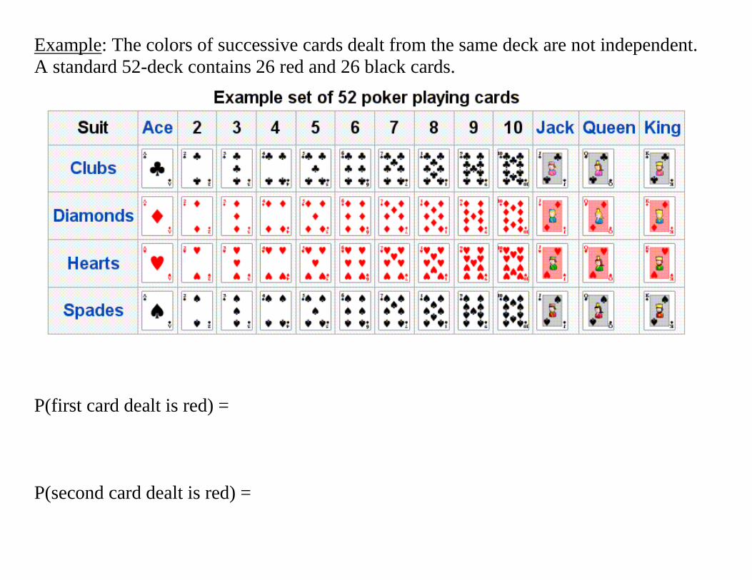
Example: The colors of successive cards dealt from the same deck are not independent.

A standard 52-deck contains 26 red and 26 black cards.

P(first card dealt is red) =

P(second card dealt is red) =

Example:

IQ Test

If you take an IQ test or other test twice in succession,

the two test scores are not independent.

The learning that occurs on the first attempt influences

your second attempt. If you learn a lot, then your second

test score might be a lot higher than your first test score.

This phenomenon is called a carry-over effect.

General Probability Rules

So far we learned five rules:

1. for any event A.

2. .

3. Addition rule: If A and B are disjoint, then

4. Compliment rule: for any event

5. Multiplication rule: If A and B are independent, then

Definition: The union of any collections of events is the event that at least one of the

collections occurs.

Addition Rule for Disjoint Events: If events A, B, and C are disjoint in the sense that no

two have any outcomes in common, then

This rule extends to any number of disjoint events.

General Addition Rule for Unions of Two Events: For any two events A and B,

Example: Deborah and Matthew are awaiting word on whether they have been made

partners of their law firm.

Deborah guesses that her probability of making partner is 0.7,

and that Matthew's is 0.5.

She also guesses that the probability

that both she and Matthew are made

partners is 0.3.

Conditional Probability

Example: There are 52 cards in the deck. Four cards are dealt, but we didn't look at them.

P(next card is ace) =

Suppose there is one ace among first four cards, then

P(next card is ace, given one of four is ace) =

P(B|A) = P(B given A) gives the probability of one event under the condition that another

event has occurred. Such probabilities are called conditional probabilities.

Example: Students of the University of Toronto received 10,000 grades last semester.

Table below breaks down these grades by which school of the university taught the

course. The schools are Liberal Arts, Engineering and Physical Sciences, and Health and

Human Services.

A B Below B Total

Liberal Arts 2,142 1,890 2,268 6,300

Engineering and Physical Sciences 368 432 800 1,600

Health and Human Services 882 630 588 2,100

Total 3,392 2,952 3,656 10,000

Consider the two events:

A = the grades comes from an engineering and physical sciences course

B = the grade is below B

A B Below B Total

Liberal Arts 2,142 1,890 2,268 6,300

Engineering and Physical Sciences 368 432 800 1,600

Health and Human Services 882 630 588 2,100

Total 3,392 2,952 3,656 10,000

Multiplication Rule: The probability that both of two events A and B happen together

can be found by

|

Example: You are at the poker table.

You want to draw two diamonds in a row.

You can see 11 cards on the table. Of these, 4 are diamonds.

Definition: When P(A) > 0, the conditional probability of B given A is

|

Note: Be sure to keep in mind the distinct roles in | of the event B whose

probability we are computing and the event A that represents the information we are

given.

Example: What is the conditional probability that a grade at the UofT is an A, given that

it comes from a liberal arts course?

A B Below B Total

Liberal Arts 2,142 1,890 2,268 6,300

Engineering and Physical Sciences 368 432 800 1,600

Health and Human Services 882 630 588 2,100

Total 3,392 2,952 3,656 10,000

Tree Diagrams

Tree diagrams are a way to draw out different possible outcomes.

A tree diagram helps us figure out the sample space for an event.

We can use a tree diagram any time we have a situation where there is more than one

possible outcome.

Example: Show the sample space for tossing one coin and rolling one die.

Example: A family has three children. How many outcomes in the sample space that

indicates the sex of the children?

Example: There are two identical bottles. One bottle contains 2 green balls and 1 red

ball. The other contains 2 red balls. A bottle is selected at random and a single ball is

drawn. What is the probability that the ball is red?

Example: Online chat rooms are dominated by the young. Teens are the biggest users. If

we look only at adult Internet users (aged 18 and over), 47% of the 18 to 29 age group

chat, as do 21% of the 30 to 49 age group and just 7% of those 50 and over. To learn

what percent of all Internet users participate in chat, we also need the age breakdown of

users. Here is it: 29% of adult Internet users are 18 to 29 years old (event ), another

47% are 30 to 49 (event ), and the remaining 24% are 50 and over (event ).

What is the probability that a randomly chosen user of the Internet participates in chat

rooms (event C)?

Bayes's Rule: Suppose that are disjoint events whose probabilities are not 0

and add to exactly 1. That is, any outcome is in exactly one of these events. Then if C is

any other event whose probability is not 0 or 1,

| |

| |

Example: What % of adult chat room participants are aged 18 to 29?

Definition: Two events A and B that both have positive probability are independent if

| .