ASSESSORS’ HANDBOOK SECTION 566

ASSESSMENT OF PETROLEUM PROPERTIES

AUGUST 1996

REPRINTED JANUARY 2015

CALIFORNIA STATE BOARD OF EQUALIZATION

SEN. GEORGE RUNNER (RET.), LANCASTER FIRST DISTRICT FIONA MA, CPA, SAN FRANCISCO SECOND DISTRICT JEROME E. HORTON, LOS ANGELES COUNTY THIRD DISTRICT DIANE L. HARKEY, ORANGE COUNTY FOURTH DISTRICT BETTY T. YEE, SACRAMENTO STATE CONTROLLER

CYNTHIA BRIDGES, EXECUTIVE DIRECTOR

AH 566 i August 1996

PREFACE

This edition of Assessors’ Handbook Section 566, Assessment of Petroleum Properties, is a complete rewrite of the original manual written in 1966 and revised in February 1972. The original manual was written under the direction of the Assessors’ Petroleum Standards Advisory Committee by four authors including one from the Board’s Assessment Standards Division (ASD). This manual is fully the product of ASD authors writing at the direction of the Board.

The goal of this handbook is to give an appraiser an understanding of the components and complexities of petroleum property appraisals. For purposes of accuracy, the appraiser should consult with qualified experts regarding any aspects of reserve estimates and petroleum engineering.

Before writing the manual, meetings chaired by Board of Equalization Member Dean Andal (Second District) were first held with industry representatives and then with assessors of petroleum-producing counties. Conflicts were identified and most were resolved. Those issues that were not resolved by meeting with industry and assessors were voted on by the Members of the Board of Equalization after hearing testimony from the interested parties and Board staff. The results of the voting are reflected as Board positions on issues in this manual.

The valuation and assessment of oil and gas properties for property tax purposes, especially under the mandates of Article XIII A of the California Constitution (Proposition 13), represents a complex and sometimes controversial challenge to county assessors. There is an ongoing need to enhance uniformity in the assessment of these valuable properties wherever they are located in the state. To that end, we submit this edition of Assessors’ Handbook Section 566, which the Board adopted on August 22, 1996.

J. E. Speed, Deputy Director Property Taxes Department State Board of Equalization

August 1996

AH 566 ii August 1996

CONTENTS

CHAPTER 1 : GEOLOGY FUNDAMENTALS .................................................. 1–1 GEOLOGY OF OIL & GAS ................................................................................................................... 1–1

Origin of Hydrocarbons ................................................................................................................ 1–1 Rock Properties ............................................................................................................................. 1–1

Porosity ..................................................................................................................................... 1–3 Permeability .............................................................................................................................. 1–3

Reservoir Fluids ............................................................................................................................ 1–5 Reservoir Water ........................................................................................................................ 1–6 Petroleum .................................................................................................................................. 1–6 Natural Gas ............................................................................................................................... 1–7

Geologic Structures ....................................................................................................................... 1–7 Hydrocarbon Traps ..................................................................................................................... 1–10

Structural Traps ...................................................................................................................... 1–11 Stratigraphic Traps ................................................................................................................. 1–11 Combination Traps ................................................................................................................. 1–11

Reservoir Drive Mechanisms ...................................................................................................... 1–11 GEOLOGIC TIME ............................................................................................................................... 1–13

CHAPTER 2 : THE PETROLEUM INDUSTRY ................................................. 2–1 IN THE UNITED STATES ...................................................................................................................... 2–1 IN CALIFORNIA ................................................................................................................................... 2–1 ECONOMICS OF THE INDUSTRY .......................................................................................................... 2–1

Worldwide Supply and Demand ................................................................................................... 2–1 Market Demand and Supply ......................................................................................................... 2–2 Working, Net Revenue, and Royalty Interests .............................................................................. 2–3

Worldwide Market .................................................................................................................... 2–4 U. S. Supply and Demand ......................................................................................................... 2–4 California Market ..................................................................................................................... 2–5

Pricing structure ............................................................................................................................ 2–5 Refinery Postings ...................................................................................................................... 2–5 Futures Contracts and Their Use .............................................................................................. 2–6

CHAPTER 3 : PRODUCTION METHODS ......................................................... 3–1 PRIMARY RECOVERY ......................................................................................................................... 3–1 CONVENTIONAL AND ENHANCED RECOVERY TECHNIQUES ............................................................. 3–2

WaterFlooding .............................................................................................................................. 3–3 Gas Injection ................................................................................................................................. 3–4 Thermal ......................................................................................................................................... 3–4

AH 566 iii August 1996

Polymer Flooding .......................................................................................................................... 3–5 Surfactant Flooding ....................................................................................................................... 3–5 Microemulsion and Micellar Flooding .......................................................................................... 3–5 Carbon Dioxide Flooding .............................................................................................................. 3–5 High Pressure Gas Drive ............................................................................................................... 3–5 Enriched Gas Drive ....................................................................................................................... 3–6 Nitrogen, Inert, and Flue-Gas Injection ......................................................................................... 3–6

CHAPTER 4 : ESTIMATION OF RESERVES AND FUTURE PERFORMANCE ..................................................................................................... 4–1 IMPORTANCE OF RESERVE ESTIMATES .............................................................................................. 4–1 DEFINITION OF RESERVES .................................................................................................................. 4–1

Proved Reserves ............................................................................................................................ 4–1 METHODS ........................................................................................................................................... 4–3

Analogy ......................................................................................................................................... 4–3 Volumetric ..................................................................................................................................... 4–4 Performance Analysis .................................................................................................................... 4–7

Material Balance ....................................................................................................................... 4–7 Performance or Decline Curves ................................................................................................ 4–8

Types of Curves .................................................................................................................... 4–8 Most Common Usage ........................................................................................................... 4–9 Economic Limit .................................................................................................................... 4–9 Hyperbolic .......................................................................................................................... 4–11 Exponential ......................................................................................................................... 4–13 Harmonic ............................................................................................................................ 4–15

Reservoir Simulation ............................................................................................................... 4–16 FUTURE PERFORMANCE ................................................................................................................... 4–16

Forecasting Production ................................................................................................................ 4–16

CHAPTER 5 : GENERAL APPRAISAL METHODS AND ASSESSMENT UNDER PROPOSITION 13 .................................................................................... 5–1 INTRODUCTION ................................................................................................................................... 5–1

“Value” for Purposes of Property Taxation .................................................................................. 5–1 The Appraisal Process ................................................................................................................... 5–2

Definition .................................................................................................................................. 5–2 Steps in the Appraisal Process .................................................................................................. 5–2

Define the Problem ............................................................................................................... 5–2 Conduct a Preliminary Survey .............................................................................................. 5–2 Collect Data .......................................................................................................................... 5–3 Process the Data into Indicators of Value ............................................................................ 5–3

AH 566 iv August 1996

Reconcile the Indicators ....................................................................................................... 5–3 Draw a Value Conclusion .................................................................................................... 5–3

THE THREE APPROACHES TO VALUE ................................................................................................ 5–3 The Comparative Sales Approach ................................................................................................ 5–4

Property Tax Rule 4 .................................................................................................................. 5–4 Market Units of Comparison .................................................................................................... 5–4 Sale of Subject Property ........................................................................................................... 5–5 Income Multipliers ................................................................................................................... 5–5

The Cost Approach ....................................................................................................................... 5–6 Replacement or Reproduction Cost .......................................................................................... 5–6 Historical Cost .......................................................................................................................... 5–7

The Income Approach ................................................................................................................... 5–7 What is the “Income Approach?” ............................................................................................. 5–7 What are the Basic Assumptions of the Income Approach? .................................................... 5–8

Value is a Function of Income ............................................................................................. 5–8 Value Depends upon the Quality and Quantity of the Income Stream ................................ 5–8 Future Income is Less Valuable Than Present Income ........................................................ 5–9

Applying the Income Approach for Property Tax Purposes .................................................... 5–9 Rule 8 ................................................................................................................................... 5–9 Discounted Cash Flow Analysis ........................................................................................ 5–11

Definition ....................................................................................................................... 5–11 Methodology .................................................................................................................. 5–11

CHAPTER 6 : PROPERTY TAX VALUATION ................................................. 6–1 PROPOSITION 13 ................................................................................................................................. 6–1 REVENUE AND TAXATION CODE SECTION 51 ................................................................................... 6–2 PROPERTY TAX RULES APPLICABLE TO PETROLEUM PROPERTIES .................................................. 6–2

Rule 2 ............................................................................................................................................ 6–2 Rule 4 ............................................................................................................................................ 6–2 Rule 8 ............................................................................................................................................ 6–2 Rule 21, Possessory Interest Definitions ...................................................................................... 6–3 Rule 22, Continuity of Possessory Interests ................................................................................. 6–3 Rule 23, Written Agreements As to the Term of Possessory Interests ......................................... 6–3 Rule 24, Possessory Interest Rights to be Valued ........................................................................ 6–3 Rule 27, Valuation of Possessory Interests for the Production of Hydrocarbons. ....................... 6–4 Rule 28, Examples of Taxable Possessory Interests ..................................................................... 6–4 Rule 121, Land .............................................................................................................................. 6–4 Rule 122.5, Fixtures ...................................................................................................................... 6–4 Rule 124, Examples [of Land] ...................................................................................................... 6–4 Rule 468 ........................................................................................................................................ 6–4

AH 566 v August 1996

SECTIONS 75 – 75.40 – SUPPLEMENTAL ASSESSMENT ....................................................................... 6–5 New Discoveries ............................................................................................................................ 6–6 New Construction .......................................................................................................................... 6–6

Additions ................................................................................................................................... 6–6 Replacements ............................................................................................................................ 6–6

Removal of Property ...................................................................................................................... 6–8 SECTION 607.5 – ASSESSABLE MINING RIGHTS OR MINERAL RIGHTS .............................................. 6–8

CHAPTER 7 : APPRAISAL OF WELLS, INSTALLATIONS, AND EQUIPMENT ............................................................................................................ 7–1 WELLS ................................................................................................................................................ 7–1 PRODUCTION EQUIPMENT .................................................................................................................. 7–1 SURFACE FACILITIES .......................................................................................................................... 7–1 APPRAISAL OF OIL FIELD PRODUCING EQUIPMENT ........................................................................... 7–2

Functional Obsolescence ............................................................................................................... 7–3 IDLE EQUIPMENT ................................................................................................................................ 7–4 APPRAISAL EXAMPLE ......................................................................................................................... 7–5

CHAPTER 8 : PETROLEUM PROPERTY APPRAISAL METHODS ............ 8–1 FORECASTING OIL PRODUCTION ........................................................................................................ 8–1 FORECASTING GAS PRODUCTION – SPECIAL ISSUES .......................................................................... 8–1

An Unconnected Gas Well ............................................................................................................ 8–1 CASH FLOW ANALYSIS ....................................................................................................................... 8–2 COMPONENTS OF A CASH FLOW......................................................................................................... 8–2

Revenues ........................................................................................................................................ 8–2 Product Prices ........................................................................................................................... 8–2 Revenue Summary .................................................................................................................... 8–2

Expenses ........................................................................................................................................ 8–3 Fixed and Variable Operating Expenses ................................................................................... 8–4 Abandonment Expenses ............................................................................................................ 8–5

State Regulations .................................................................................................................. 8–5 Accounting For Abandonment Expenses ............................................................................. 8–6

Environmental Expenses ........................................................................................................... 8–6 Benchmarking ........................................................................................................................... 8–6 Royalty Deductions ................................................................................................................... 8–6 Expense Summary ..................................................................................................................... 8–7

Value Determination ..................................................................................................................... 8–7 Discount Rates .......................................................................................................................... 8–7 Risk ........................................................................................................................................... 8–8

AH 566 vi August 1996

Income Multipliers ................................................................................................................. 8–11 Measures of Success ............................................................................................................... 8–11

TAXABLE VALUE ............................................................................................................................. 8–12 Current Market Value ................................................................................................................. 8–12 Factored Base Year Value .......................................................................................................... 8–12

APPENDIX A: GLOSSARY OF TERMS.............................................................................................. 1 APPENDIX B: SUMMARY OF RELATED COURT CASES ............................................................ 1 APPENDIX C: DERIVATION AND ESTIMATION OF DISCOUNT RATES USED IN

DISCOUNTED CASH FLOW ANALYSIS........................................................................................... 1 Introduction ....................................................................................................................................... 1 Present Value and Discounted Cash Flow Analysis ......................................................................... 1

The Concept of Present Value ...................................................................................................... 1 Discounted Cash Flow Analysis ................................................................................................... 1 Terminology ................................................................................................................................. 3

Deriving Discount Rates from Sales Data ........................................................................................ 4 Introduction .................................................................................................................................. 4 Sales Data ..................................................................................................................................... 4 Anticipated Income and Expenses and Cash Flow Projections .................................................... 4 Treatment of Inflation in Cash Flows ........................................................................................... 5 Computation of the IRR or Discount Rate ................................................................................... 6

Checking the Validity of Discount Rates Using Market Surveys ..................................................... 6 Deriving Discount Rates Using the Band of Investment or Weighted Average Cost of Capital ..... 7

Band of Investment or Weighted Average Cost of Capital Defined ............................................ 7 Estimating Capital Structure Weights ...................................................................................... 8 Estimating the Cost of Debt ..................................................................................................... 8 CAPM Overview ...................................................................................................................... 8 A Few of the Difficulties in Applying CAPM ....................................................................... 10

Conclusion and Summary ............................................................................................................... 10 Market-Derived Discount Rates ................................................................................................. 10 Market Surveys ........................................................................................................................... 11 Band of Investment or Weighted Average Cost of Capital ........................................................ 11

APPENDIX D INFLATION TRENDS .................................................................................................. 1 APPENDIX E – OIL PRICE ................................................................................................................... 1

WTI 1946–1995 ................................................................................................................................ 1 Recent WTI and Kern River Crude Prices 1980–1995 ..................................................................... 2

APPENDIX F: PETROLEUM ENGINEERING AND PRODUCTION SYMBOLS, ABBREVIATIONS AND DEFINITIONS ............................................................................................. 1 APPENDIX G: PRESENT WORTH FACTORS – MID–YEAR ........................................................... 1 APPENDIX H: FORMS & WORKSHEETS ......................................................................................... 1

AH 566 vii August 1996

APPENDIX I: SELECTED STATUTES AND PROPERTY TAX RULES ........................................... 1 Revenue and Taxation Code .............................................................................................................. 1 Property Tax Rules .......................................................................................................................... 21

BIBLIOGRAPHY ................................................................................................................................. 1

AH 566 1–1 August 1996

Chapter 1 : GEOLOGY FUNDAMENTALS

GEOLOGY OF OIL & GAS

ORIGIN OF HYDROCARBONS Under generally accepted geologic theory, oil and gas are believed to have originated from organic matter deposited in sedimentary rocks. Pressure, temperature, and bacterial action over long periods of time reduce the organic material into carbon and hydrogen molecular combinations called hydrocarbons. The organic material from which the oil is derived probably consisted of single-celled plants, blue-green algae, and single-celled animals which lived in aquatic environments 540 million years ago.

The rapid burial of these organisms within sediments preserved them for later biological, chemical, and physical changes into a material called kerogen.1 Kerogen is a product of early bacterial alteration that is dark-colored and insoluble. During this transformation stage, mostly methane gas is generated. Continuing sedimentation after burial of these organisms increases the depth of burial, and with increasing depth there is an increase in temperature.

Temperature change with depth is known as the geothermal gradient. The U.S. Geological Survey publishes geothermal gradient maps for the United States. Globally, the average increase in temperature with depth ranges from about 0.57 degrees F to about 1.7 degrees F for each 100 feet. California’s gradients tend to be more toward the higher end of the range because of their location along a major plate boundary and its status of being geologically active as a result of the forces of plate tectonics. However, even in California the gradients vary considerably from one area to another. The best way to determine the gradient in any particular area is to consult the U.S. Geological Survey gradient map for California.

The production of multiple petroleum compounds is a direct consequence of the thermal degradation and cracking process. Cracking is the breaking up of the hydrocarbon molecules into lighter molecules. The process generally occurs at depths of 2,500 to 16,000 feet and at temperatures of 150 to 300 degrees F. Temperatures reached by potential petroleum source rocks can be determined by the degree of darkening of fossil pollen grains and the color changes in a type of extinct marine invertebrate fossil.

ROCK PROPERTIES Petroleum and natural gas do not exist in underground lakes, rivers, or caverns, but within the void space of certain kinds of rocks. For commercial deposits of these substances to accumulate there must be:

1 Words and phrases shown in bold italic (e.g. kerogen) are defined in Appendix A, Glossary of Terms.

AH 566 1–2 August 1996

• A source rock in which the hydrocarbons were formed

• A reservoir rock containing porosity and permeability (discussed below) where the hydrocarbons may migrate and accumulate

• A trap which will restrict further movement of the hydrocarbons so they may accumulate in commercial quantities

The accumulation of oil and gas in nature and the migration of these substances into a trap rock almost exclusively occurs in a single rock type known as sedimentary rock. Rocks are generally classified according to their origin. They fall into three simple classifications: Igneous, Sedimentary, and Metamorphic.

Accumulations of petroleum occur in metamorphic and igneous rocks usually because of porosity resulting from fracturing; however, such reservoirs are relatively rare. A complete discussion of igneous and metamorphic rocks can be found in Assessors’ Handbook Section 560, Assessment of Mining Properties.

Sedimentary rocks are all of secondary origin, deriving from the disintegration of older rocks through the action of weathering. A sedimentary rock could consist of the remnants and redeposition of a weathered igneous, metamorphic, or sedimentary rock.

Sedimentary rocks are characterized by a parallel or bedded structure, similar to a stack of books. The layers may vary in thickness, and the individual grains of the materials making up the rock may show considerable variation in composition and size. When particles of sand varying in size from 0.02 to 2.0 mm become consolidated, sandstone results. (There are 25.4 mm to an inch.)

Sedimentary rocks form widely extended deposits which are generally without great vertical dimensions, especially when compared with some of the massive igneous formations. Such deposits can be many thousands of feet thick. Sedimentary rocks are classified in the field based on origin as to:

• Mechanical sediments such as shale, sandstone, and conglomerate.

• Chemical sediments such as gypsum, salt, and limestone.

• Organic sediments such as coal or limestone.

• Evaporite sediments such as salt and anhydrite.

Mechanically deposited sediments are those that are transported from one place to another by water, wind, or glaciers. Chemically deposited sediments are those that are precipitated from solution when certain chemical solutions come in contact with each other. Organic sediments, of course, are the remains of once living organisms. Limestone can be of a chemical or organic origin.

AH 566 1–3 August 1996

Sedimentary rocks carry petroleum and natural gas because petroleum was formed in the layers. They are typically porous, allowing the tiny pore spaces between the grains to store the oil, gas, and water. Because these pores can be interconnected, liquids can move through the rock. The interconnection of the pores is called permeability. The ability of sedimentary rocks to be porous and permeable make them incredibly valuable to man. Porosities in reservoir rocks may range from about 5 percent to 30 percent or more. The lower porosities are more apt to occur in carbonate reservoirs, which are nearly non-existent in California but are common in other parts of the country.

Porosity Porosity is the void space in a rock formation. This can be filled with gas, water, or oil. To help visualize porosity think of a glass filled to the top with marbles. Though the glass is full it is still capable of holding fluid. The spaces between the marbles can be filled with water. The volume of water compared to the total volume of the glass is the porosity. It is generally expressed as a percentage of the total volume. A rock with a porosity of 20 percent is 80 percent dense rock material and 20 percent void space. Porosity is typically designated by the Greek symbol “phi” (φ).

Porosity is of two types: primary porosity, which is a result of depositional factors; and secondary porosity, which is a result of post-depositional or induced factors occurring as a result of deformation.

Permeability Permeability is the measure of a rock’s resistance to the flow of fluids through it. A high permeability formation is very conducive to flow. A low permeable formation is described as being tight. Permeability is mostly dependent on the size and shape of the pores and by the size, shape, and packing of the grains making up the rock. To visualize how packing can affect both porosity and permeability, imagine eight marbles of equal size packed into a square box equal to the diameters of two marbles. This kind of packing arrangement yields a porosity of 47.6 percent and is called cubic packing. Now take the marbles out of the box, place four marbles back in the bottom of the box, and lay a marble on top and in the center of the four marbles. This kind of packing yields a porosity of 25.96 percent and is called rhombohedral packing. If these same marbles were not perfectly round, but angular, you can visualize the effect it could have on available pore space.

While shale was earlier identified as a sedimentary rock and may contain very high porosities, it lacks permeability. Although rare, some shales do contain petroleum in the form of bitumen, a solid form of petroleum. There are extensive deposits of bitumen-containing shale deposits (oil shale) in some of the western states such as Colorado and Wyoming. For these types of deposits the mineral is mined and processed to extract the petroleum. Similar projects have been conducted in California. The Antelope Shale pilot project in the McKittrick field recovered 21,400 barrels of oil in the four years it was in operation.

AH 566 1–4 August 1996

In order for the individual grains of a sedimentary rock to be held together, they are "cemented" by nature with various cementing minerals that vary from one sedimentary rock to another. Typically, the cementing material is silica or calcium carbonate, but it may also be iron oxides, barite, anhydrite, zeolites, and clay minerals. The cement holds the grains in place, but there is still pore space available and permeability. However, the amount of cementing material can have an adverse affect on porosity.

To visualize a sedimentary rock as a fluid reservoir, imagine a bucket filled with sand. Then slowly add water. You could probably add about a half a bucketful of water or more depending on the size and shape of the sand grains. The size and shape of the grains is very important. More angular grains tend to increase the porosity. Increases in the distribution of various particle sizes, i.e., poor sorting of the grain sizes, decreases porosity.

Petroleum engineers and geologists speak in terms of total porosity and effective porosity. Because some of the cementing material may seal off some of the pores, they may not contribute to fluid recovery. The porosity that does contribute to fluid recovery, therefore, is known as effective porosity. It is the effective porosity that contains the mobile fluids.

Carbonate rocks, such as limestones and dolomites, have complex pore systems since they are of chiefly chemical origin. Many limestones and dolomites have porosity because they are oolitic, that is, they are composed of minute spherical particles. Limestone and dolomitic petroleum reservoirs typically have lower porosities and permeabilities than sandstone reservoirs.

Petroleum geologists frequently speak of “dirty” sands. This is a reference to sand containing silt or clay materials which reduce the porosity.

Porosities of reservoir rocks may be determined by core sampling and laboratory analysis or by well logging where an electronic or electrical tool is lowered into the well before it is cased with well casing. After casing, a “neutron log” can be used.

Organic sediments consist of the skeletal remains of once living organisms. Examples of these are fossiliferous limestone and diatomaceous earth. Diatomaceous earth consists of the microscopic remains of fossil diatoms, a microscopic plant which has an outer skeleton of hydrated silica and which inhabits both fresh and salt water.

Evaporite deposits, such as salt beds or potash beds, are usually contained in ancient lakebeds where water has evaporated leaving behind chemicals that were contained in solution.

AH 566 1–5 August 1996

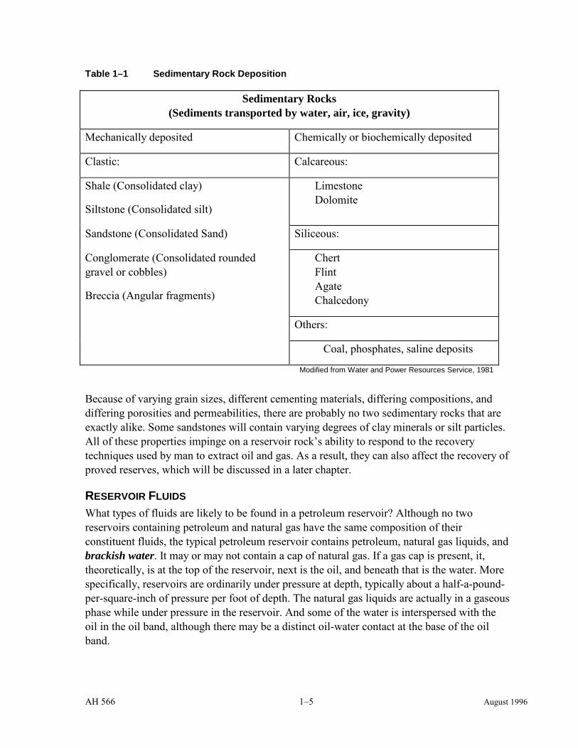
Table 1–1 Sedimentary Rock Deposition

Sedimentary Rocks (Sediments transported by water, air, ice, gravity)

Mechanically deposited Chemically or biochemically deposited

Clastic: Calcareous:

Shale (Consolidated clay)

Siltstone (Consolidated silt)

Limestone Dolomite

Sandstone (Consolidated Sand) Siliceous:

Conglomerate (Consolidated rounded gravel or cobbles)

Breccia (Angular fragments)

Chert Flint Agate Chalcedony

Others:

Coal, phosphates, saline deposits

Modified from Water and Power Resources Service, 1981

Because of varying grain sizes, different cementing materials, differing compositions, and differing porosities and permeabilities, there are probably no two sedimentary rocks that are exactly alike. Some sandstones will contain varying degrees of clay minerals or silt particles. All of these properties impinge on a reservoir rock’s ability to respond to the recovery techniques used by man to extract oil and gas. As a result, they can also affect the recovery of proved reserves, which will be discussed in a later chapter.

RESERVOIR FLUIDS What types of fluids are likely to be found in a petroleum reservoir? Although no two reservoirs containing petroleum and natural gas have the same composition of their constituent fluids, the typical petroleum reservoir contains petroleum, natural gas liquids, and brackish water. It may or may not contain a cap of natural gas. If a gas cap is present, it, theoretically, is at the top of the reservoir, next is the oil, and beneath that is the water. More specifically, reservoirs are ordinarily under pressure at depth, typically about a half-a-pound-per-square-inch of pressure per foot of depth. The natural gas liquids are actually in a gaseous phase while under pressure in the reservoir. And some of the water is interspersed with the oil in the oil band, although there may be a distinct oil-water contact at the base of the oil band.

AH 566 1–6 August 1996

Reservoir Water Petroleum engineers believe that most trap rocks first contained water before the oil migrated into them. As such, the grains making up the rock are water wet or are surrounded by a film of water. This water in the pore spaces is known as connate water because it was deposited along with the sediments. Typically, such deposition occurred in a marine environment, which accounts for the fact that the water is brackish. Generally speaking, salinities increase with depth. Interstitial water is merely a generic term denoting the water in the pore space of a rock and does not imply whether the water was there initially or whether it migrated. In some instances, reservoir water salinity may approximate that of today’s oceans, (about 35 parts-per-thousand of dissolved solids) and/or may contain other contaminates, requiring special handling for its disposal.

Petroleum Petroleum is composed primarily of hydrocarbons (hydrogen and carbon atoms). Nearly all crude oil ranges from 82 to 87 percent carbon by weight and 12 to 15 percent hydrogen. Most crude oils contain trace quantities of oxygen, nitrogen, salt, and heavy metals (vanadium and nickel are the most common), as well as sulfur compounds. Sulfur content generally increases with decreasing API gravity. Crude oils contain several thousand different organic compounds of hydrocarbons.

Crude oils can be classed into three types: paraffin, naphthene (asphaltic), and aromatic. Paraffin based crudes contain a high amount of wax (paraffin), and naphthene based crudes contain a large amount of naphthenes. It is the naphthene based crudes that are predominant in California and are also a superior source of motor fuel. Paraffin based crudes are more predominant in the eastern part of the United States and Texas. Aromatic crudes account for only a small percentage of produced crudes; and, their chief constituent is benzene.

The makeup of the crude is one factor affecting its recoverability. The petroleum’s density as measured in the laboratory is known as the API gravity (American Petroleum Institute standard). The lower the API gravity, the more viscous the crude oil. California crudes generally range in API gravity from about 8 to 35, with 8 being the most viscous. These lower API gravity oils are commonly found in the southern San Joaquin Valley. API gravities less than 10 are actually heavier than water. The equation below shows the formula for calculating the API gravity of oil.

API°= −141 5 131 5.

. ..

s g Equation 1–1

Where:

s.g. = Specific Gravity at 60 degrees F

Crude oil API gravity directly affects the value of the produced crude oil. Major crude oil buyers post their price offerings for purchase of a barrel of crude oil based on its API gravity.

AH 566 1–7 August 1996

These buyers also specify maximum water content and contaminant allowances such as sand. In the United States, a barrel consists of 42 gallons. A barrel of API 30º gravity oil weighs about 306 pounds. In many countries, crude oil is measured in metric tons equal to about 7.2 U.S. barrels.

Natural Gas Natural gas often coexists in crude oil reservoirs and frequently provides the pressure to drive the crude oil to the surface through wells. This gas is often called “associated gas” because it is found in the presence of crude oil and it frequently contains some light liquids when brought to the surface. Natural gases often consist of methane, ethane, and propane that may exist in the gaseous phase in the reservoir. Pentane and other heavier compounds may be present along with large quantities of hydrogen sulfide and/or other organic sulfur compounds. Many natural gas liquids (NGL) may be extracted from the produced associated gas on or near the lease before the products are sold to the refinery. NGLs represent an additional revenue stream for the property.

Large quantities of natural gas are also produced from reservoirs that do not contain crude oil. This gas is usually referred to as “non-associated gas.” Non-associated gas fields are common in the Sacramento Valley of Northern California. This gas may contain little, if any, wet fractions.

Natural gas is sold based on its heating value measured in BTUs (British Thermal Units). Prior to 1956, it was defined as the amount of heat required to raise the temperature of one pound of water 1º F. It was changed because it was dependent on the initial temperature of the water. Now it is defined as approximately equal to 1,055 joules or 252 gram calories. The greater the methane content of the gas, the higher the BTU value.

Natural gases frequently contain other constituents such as nitrogen and carbon dioxide, both of which are noncombustible. Other contaminants may also be present. The noncombustible gases, if present in significant amounts, must be removed, thereby raising the heating value and market value of the gas.

With production, dry gas reservoirs will decline in pressure. This drop may be so great as to necessitate the compression of the gas in order for it to be able to enter the collection pipeline. Various stages of compression may be necessary. Compression is a cost to the operator or producer of the gas. Some of the produced gas may be used as fuel for the compressors.

GEOLOGIC STRUCTURES The existence of a geologic structure is necessary for the accumulation of petroleum. The study of geologic structures is a complex subject which is discussed only briefly here.

AH 566 1–8 August 1996

Diastrophism is the term applied to all movements of the solid parts of the earth with respect to each other. These movements are generally slow and evolve over periods of thousands or millions of years. The diastrophic processes may be classified as shown in Table 2.

Table 1–2 Diastrophic Processes

Uplift — elevation of portions of the earth's crust

Subsidence — depression of portions of the earth's crust

Plate tectonics — crustal plates that move with respect to each other, both sideways and by slipping underneath each other.

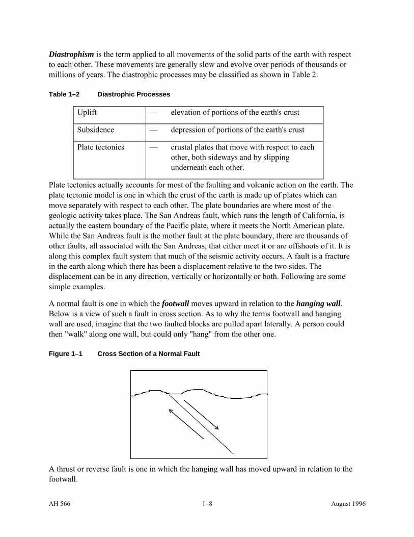
Plate tectonics actually accounts for most of the faulting and volcanic action on the earth. The plate tectonic model is one in which the crust of the earth is made up of plates which can move separately with respect to each other. The plate boundaries are where most of the geologic activity takes place. The San Andreas fault, which runs the length of California, is actually the eastern boundary of the Pacific plate, where it meets the North American plate. While the San Andreas fault is the mother fault at the plate boundary, there are thousands of other faults, all associated with the San Andreas, that either meet it or are offshoots of it. It is along this complex fault system that much of the seismic activity occurs. A fault is a fracture in the earth along which there has been a displacement relative to the two sides. The displacement can be in any direction, vertically or horizontally or both. Following are some simple examples.

A normal fault is one in which the footwall moves upward in relation to the hanging wall. Below is a view of such a fault in cross section. As to why the terms footwall and hanging wall are used, imagine that the two faulted blocks are pulled apart laterally. A person could then "walk" along one wall, but could only "hang" from the other one.

Figure 1–1 Cross Section of a Normal Fault

A thrust or reverse fault is one in which the hanging wall has moved upward in relation to the footwall.

AH 566 1–9 August 1996

Figure 1–2 Cross Section of the Earth Showing a Thrust Fault

A lateral fault is one in which the movement has occurred laterally to one side with respect to the other. Below is an overhead view of a lateral fault similar to the San Andreas fault where the two sides move in opposite directions.

Figure 1–3 Overhead View of a Lateral Fault

Because most fault movement occurs slowly and is quickly overtaken by erosion, the effect of the movement is usually hidden to the casual observer. Nevertheless, the fault is still there, and it could be quite active. Faults are important economically since they are sometimes filled with minerals derived from underlying magmas and may act as traps for petroleum and natural gas.

Fissures are small fractures in rock caused by rupturing that sometimes occurs during folding from lateral compressional forces, or from pressures exerted below the rock from upwelling magmas. Folding of rocks is another very common phenomena. There are folds called anticlines and synclines. These patterns of folds in nature are constantly repeated, but they are not perfectly symmetrical and may even be faulted.

AH 566 1–10 August 1996

Figure 1–4 Beds of Sandstone into an Anticline Beneath the Earth's Erosional Surface

The layers of sedimentary rock are separated by what geologists call bedding planes. These are the division planes that separate the individual layers. Bedding planes are found only in sedimentary rock types and represent changes in deposition over time.

HYDROCARBON TRAPS Exploration for hydrocarbons occurs in the sedimentary basins of the world. A sedimentary basin is a depressed, sediment filled area, frequently great in areal size, where the depth of sediments can range to 20,000 feet or more. It is in these types of settings where nearly all of the world’s oil has been found. Worldwide, about 600 sedimentary basins are known to exist, and about 160 of these have been productive. In another 240, no significant commercial discoveries have been made, and the remainder are located in environments too difficult to explore, such as polar regions and submerged continental margins. In California there are 10 productive basins (see Table 3).

Table 1–3 Productive California Basins

Cuyama Eel River

Half Moon Los Angeles

Sacramento Salinas

San Joaquin Santa Maria

Sonoma Ventura

In order for petroleum to accumulate, some type of trapping mechanism must exist. There are three classifications of traps: structural, stratigraphic, and combination.

AH 566 1–11 August 1996

Structural Traps Structural traps are traps resulting from earth movement. They consist principally of two types: anticlinal and fault.

Anticlinal traps result from tectonic forces that reshape the earth’s crust. As noted earlier in this chapter, an anticline is an upward fold. Hydrocarbons become trapped in the apex of the fold. Traps can only occur in the presence of a trapping medium, such as a seal by a denser, impermeable cap rock such as shale. About 80 percent of the world’s petroleum has been found in this type of trap.

Fault traps occur as a result of rock fracture where a displacement of strata forms a barrier to the upward migration of hydrocarbons. In such situations an impermeable bed is brought into contact with a bed containing hydrocarbons. Active seismic activity can adversely affect the traps that are formed, as well as production operations.

Stratigraphic Traps Stratigraphic traps are associated with sediment deposition or erosion. These traps are confined on one or more sides by low or impermeable zones. Stratigraphic traps are also commonly affected by structure (see combination trap below). Changes in depositional features, such as the pinchout of a sand along the edges of a marine basin environment or changes in depositional materials, may lead to rapid porosity and permeability pinchouts that result in a trap. Stratigraphic traps are as varied as nature itself.

Combination Traps A combination trap is merely one that has elements of both a structural trap and a stratigraphic trap, such as the pinchout of a reservoir sand on the limb of an anticline.

Examples of various types of traps can be found in California Oil and Gas Fields, Maps and Data Sheets, a publication of the California Division of Oil and Gas.

RESERVOIR DRIVE MECHANISMS Upon the initial discovery and production of petroleum reservoirs, there is usually sufficient formation pressure to force the crude oil into the well, and sometimes this pressure is great enough to force the crude to the surface. If it reaches the surface, the pressure is sufficient to overcome the weight of the fluid column in the well bore. The more gas contained in the fluid column, the less formation pressure necessary to reach the surface. Where the oil is able to reach the surface on its own, without the necessity for pumping, the well is said to “flow.”

There are basically two kinds of pressure existing in a porous rock at depth: hydrostatic and internal. Hydrostatic pressure exists in the rock because of its burial under rock overburden. Internal pressure exists because of the pressure wielded by the fluids and gases in the void spaces of the rock.

AH 566 1–12 August 1996

The recovery of oil is a process of displacement because oil does not have an intrinsic ability to discharge itself from the reservoir. A displacing agent must be present. Usually the displacing agents are gas or water, or both, which may be naturally available in the reservoir. Gravity is also a significant agent of mobility in some reservoirs. The type of drive mechanism is important. To a great extent, the amount of oil that may be ultimately recovered depends on the efficiency of the dominant drive mechanism.

Internal pressure is related to one or more of the following pressure mechanisms (primary recovery) that may be naturally present in the reservoir:

• Dissolved-gas drive

• Gas-cap drive

• Water drive

• Gravity drainage

Other forces may also affect oil production, such as the elastic expansion or compaction of the reservoir. Nowhere is this more in evidence than in the Wilmington field in the Los Angeles basin where a considerable amount of subsidence has occurred as a result of oil withdrawals from the field over decades of time. It occurs with greater frequency in areas where the rock formations are poorly consolidated.

In the dissolved-gas drive mechanism, gas is liberated from solution in the oil as the pressure in the reservoir is reduced as a result of production. Oil recovery by dissolved-gas drive is an inefficient production mechanism. As the gas is dissipated from solution, depletion occurs throughout the reservoir.

In the gas-cap drive mechanism, the displacing agent is gas from the free gas cap that overlies the oil zone. As oil is produced, the gas cap expands and forces the oil to the well bore which is an area of reduced pressure. This drive mechanism is generally less efficient than water drive but more efficient than solution-gas drive.

Where water drive is the operative mechanism, water encroaches into the oil bearing zone from a neighboring or nearby aquifer. As a result of oil production, pressure is reduced, especially in the vicinity of the well bore, and the water flows toward the area of reduced pressure, sweeping the oil along with it.

In the above described mechanisms, gravity may also exert an effect. In fact, whenever there is a vertical component to fluid movement, gravity may be at work in influencing fluid motion. Sometimes gravity is the dominant mechanism, particularly in a closed reservoir uninfluenced by neighboring aquifers. Gravity drainage is generally the most efficient drive mechanism.

There are many factors that influence the recovery of oil, as noted. The following is a list of those factors which should be considered in evaluating a petroleum property:

AH 566 1–13 August 1996

Table 1–4 Factors Influencing Oil Recovery

• Porosity, permeability, and both interstitial water and connate water saturation.

• The geologic structure along with the continuity of the producing formation and its degree of uniformity.

• Properties of the formation oil, such as the viscosity, amount of gas in solution, and shrinkage.

• The degree to which the operator performs proper controls, to the extent that they may be effective, in the rate of production of gas, oil, and water, including control of expulsive forces.

• Well conditions and maintenance.

• Location of the well(s) with respect to the geology of the reservoir.

GEOLOGIC TIME

As previously noted with regard to geologic time, all the geologic processes have been at work throughout geologic history. Whether fault movement, uplift, subsidence, folding, or sedimentary deposition, it occurs slowly and imperceptibly. Plate movement varies from only about one-half inch per year to five inches per year, at the most. A motion of just two inches a year adds up to 30 miles in only one million years. Some plates have been in motion for 100 million years for a total movement of 3,000 miles over that period of time.

Figure 1–5 is a geologic time chart showing geologic eras and periods that correlate with producing formations throughout the world. Only the Cretaceous period of the Mesozoic Era, and the Paleocene, Eocene, Oligocene, Miocene, Pliocene, and Pleistocene are, or have been, significantly represented in California oil fields.

AH 566 1–14 August 1996

Figure 1–5 Geologic Time Chart

Era

Period

Epoch

Age (in Millions of Years)

Cenozoic Quaternary Tertiary

Pliocene Miocene Oligocene Eocene Paleocene

Recent 1.6

66.4

Mesozoic Cretaceous Jurassic Triassic

66.4

245

Paleozoic Permian Carboniferous Devonian Silurian Ordovician Cambrian

245

540

Pre-Cambrian Late Pre-Cambrian Early Pre-Cambrian

540 3960

AH 566 2–1 August 1996

Chapter 2 : THE PETROLEUM INDUSTRY

IN THE UNITED STATES

Writings of early American explorers contain numerous references to petroleum seeps and springs. During the late 1700s and early 1800s, numerous accounts of Indians using petroleum products for medicinal purposes mirrored their use in Europe and by the new settlers. Pharmaceutical demand, however, was the only principal use. Oils for lighting and other lubricants were primarily provided by whale oils. Most petroleum-based medicines were sold in half pint bottles; therefore a barrel of production from a spring or a trench went a long way.

The first successful oil well was drilled by Colonel E. L. Drake near Titusville, Pennsylvania in 1859. The entrepreneur behind the first commercial oil well was George Bissell. Bissell knew that petroleum was flammable and believed that it had use as an illuminate. This belief helped establish the petroleum industry. Natural gas was already being used for street lights in some areas. Early studies indicated to Bissell and his investors that “rock oil” could be distilled into kerosene. There were already refineries that were manufacturing kerosene from asphalt and coal. The success of the Drake well sparked the beginning of the boom and bust cycles that are part of the industry today.

IN CALIFORNIA

In 1854 gas produced from a water well was being used to light the courthouse building in Stockton, California. Exploration for petroleum began in the 1860s with limited success. In 1910 California was the leading producer in the country and the world, producing that year over 73 million barrels of oil.

ECONOMICS OF THE INDUSTRY

Many factors influence production practices in an oil or gas field. Demand, price, availability, competition, remaining economic life, production methods, and production rate must all be considered. While these factors can change on a daily basis, petroleum properties are assessed each year on the lien date, on the date of a “change in ownership,” or on the date of completion of new construction. Changes in value occurring after the lien date due to economic factors are not recognized unless there is an intervening change in ownership.

WORLDWIDE SUPPLY AND DEMAND Control of petroleum resources has led to the economic rise and fall of many nations. The Japanese attack on Pearl Harbor was part of its larger plan to control the petroleum resources of Indonesia. In the 1930s, Japan imported 80 percent of its petroleum from the United States. The Japanese drive into Southeast Asia in 1940 was an effort to secure its supply in

AH 566 2–2 August 1996

the event of a U.S. embargo, which did occur in the summer of 1941. The Japanese attack on Pearl Harbor was meant to protect the flank of Japan’s invasion into Southeast Asia.

Adolf Hitler’s goals in the invasion of the Soviet Union were the farmlands of the Ukraine and the oil fields of the Caucasus. With these two areas under German control, Hitler felt that he would have the resources to make the Third Reich impregnable. Hitler also sought to remove the Soviets as a threat to Rumania’s oil fields, a German ally.

Today petroleum and its control continues to influence the position of countries in worldwide politics. In 1973, Arab nations embargoed petroleum exports to the United States in response to its support of Israel after the Yom Kippur War. This caused supply disruptions and led to lines at gas stations as drivers kept their tanks “topped off” to avoid paying higher prices later in the week. The Iranian revolution in 1979 again raised the specter of fuel shortages and the return of gas lines. Oil price peaked near $40 per barrel in 1981 and steadily began to decline as the economics of production changed with changes in supply. At the end of 1985 many OPEC (Organization of Petroleum Exporting Countries) countries were exceeding their quotas. Saudi Arabia had been considered as the swing producer of the group; however, in order to prop up prices, Saudi production had declined to historic lows and revenues fell below the needs of the country. The ruling Saudi family decided that Saudi Arabia was no longer going to sacrifice so that other OPEC members could build market share by exceeding their quotas. The Saudis opened the valves and started a price war that plunged the price from $28 per barrel to $10 per barrel.

The politics of oil has dominated the 1980s and early 1990s. Sadam Hussein’s invasion of Kuwait was, in part, his response to overproduction by Kuwait and other members of OPEC that had caused the price of oil to remain below the official OPEC marker price. Hussein annexed all of Kuwait, claiming that it was a historic province of Iraq that had been illegally taken away by Western imperialists.

Hussein, however, drastically underestimated the perceived threat this action created for the international community. Many questioned whether or not Hussein would be satisfied with Kuwait or if his next target was Saudi Arabia. Opposition was quickly organized by the United Nations. The uncertainty following the invasion caused oil prices to quickly climb above $35 per barrel. Prices retreated after a short time, however, when it was realized that even with an embargo against Iraqi and Kuwaiti production, other producers were able to satisfy world demand.

MARKET DEMAND AND SUPPLY The petroleum market represents a balance between supply and demand that is not easily controlled by any one party or cartel. As a commodity, California oil and gas prices are subject to and affected by fluctuations in national, regional, and worldwide supply and demand, resulting in continuous adjustments in price. Deregulation in and of itself will not cause prices to go up or down. Commodities allowed to trade on an open market are subject to forces of supply and demand.

AH 566 2–3 August 1996

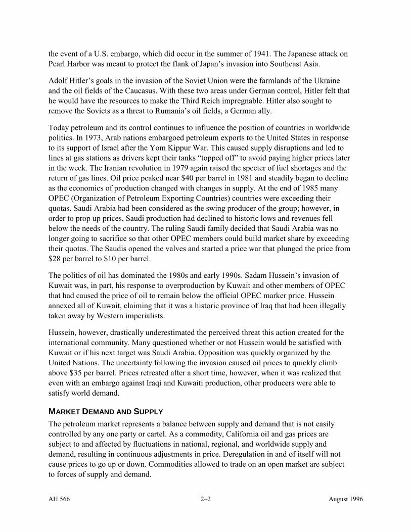
Figure 2–1 History of Price Change for West Texas Intermediate Crude Oil

1/1/46 1/1/50 1/1/54 1/1/58 1/1/62 1/1/66 1/1/70 1/1/74 1/1/78 1/1/82 1/1/86 1/1/90 1/1/94-0.4

-0.2

0

0.2

0.4

0.6

0.8

1

1.2

1.4

Per

cent

Rea

l Pric

e C

hang

eReal Change in WTI Oil Price 1946–1994

WORKING, NET REVENUE, AND ROYALTY INTERESTS Mineral interests represent a unique right to land. Ownership or control of a mineral right gives the exclusive right to extract from the land its mineral content. The owner of the mineral rights on a property may or may not be the owner of the surface rights. Mineral interests can be bought and sold separately from the surface rights. They can be further divided by depth, type of mineral, or partial ownership. Many mineral right owners do not have the financial and technical resources or the desire to properly develop their mineral interests and therefore lease to someone who does.

Ownership of the mineral rights grants the holder reasonable access to the land to allow development of the minerals. The mineral interest holder is liable for any damage to the surface caused by the exploration, development, and production operations on the property. The lessor usually will retain a royalty interest as compensation for the use of the mineral rights. The lessee has a leasehold interest in the property, often called a “working interest.” The working interest holds the exclusive rights — pays essentially all of the costs — to explore, develop, and produce the property. The proceeds the working interest receives from the sale of any production is called the “net revenue interest.” The net revenue interest receives profits less any royalties paid. The royalty owner receives a percentage of the

AH 566 2–4 August 1996

production either in kind (actual production) or from the gross proceeds, free and clear of any operating costs. The royalty owner may incur some administrative costs, in proportion to their percentage of the enhanced recovery costs for fuel and property taxes.

Since at the time an initial lease is signed there is usually little information about the productive capacity of the property, the mineral owner also may receive a one time bonus payment and an annual rent until the property has been drilled or the lease quitclaimed. For property tax purposes, the present value of the bonus and rental payments generally represent the current value of the property, although the lease could be terminated before production occurs. The lessees value resides in his exclusive rights to explore for and produce any oil and/or gas he may find. Typical primary terms for leases are five or ten years. Many leases also contain a clause that encourages the company to begin drilling as soon as possible. Generally the rental rates will increase as the term of the lease advances. Once production has been established the lease will remain in effect until production ceases. Most leases have a clause that if production ceases on a lease, the operator has 60 days to begin reworking the well or start drilling a new one.

Worldwide Market Present worldwide estimates are that there is enough oil to meet current demands for the next 45 years. New discoveries of gas continue to be developed; and, the current political climate is that the fuel of choice for much of our national energy needs is natural gas.

While the United States was a dominating factor in worldwide oil production early in the century, the country is now a net importer of crude oil and oil products. The leading producer group has become the Organization of Petroleum Exporting Countries (OPEC). Members of OPEC have agreed, in theory, to restrict production from their fields in order to support prices and maintain market share. In actual practice, each country does what is best for its own interests. Supplies from non-OPEC countries have been increasing through the later half of the 1980s and early 1990s.

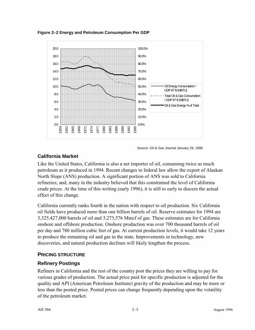
U. S. Supply and Demand The United States is the largest consumer of energy in the world and a net importer of oil. While U.S. consumption has increased over the last several years, so has efficiency. Since 1972, total oil and gas energy consumption per Gross Domestic Product (in 1987 dollars) has decreased from 17.9 to 10.2 Thousand BTU/dollars. Oil and gas make up a smaller share of the total energy used in the United States each year. See Figure 2–2.

AH 566 2–5 August 1996

Figure 2–2 Energy and Petroleum Consumption Per GDP

0.0

2.0

4.0

6.0

8.0

10.0

12.0

14.0

16.0

18.0

20.0

1959

1962

1965

1968

1971

1974

1977

1980

1983

1986

1989

1992

1995

0.0%

10.0%

20.0%

30.0%

40.0%

50.0%

60.0%

70.0%

80.0%

90.0%

100.0%

Oil Energy Consumption /GDP 87 $ (MBTU)Total Oil & Gas Consumption/ GDP 87 $ (MBTU)Oil & Gas Energy % of Total

Source: Oil & Gas Journal January 29, 1996

California Market Like the United States, California is also a net importer of oil, consuming twice as much petroleum as it produced in 1994. Recent changes to federal law allow the export of Alaskan North Slope (ANS) production. A significant portion of ANS was sold to California refineries; and, many in the industry believed that this constrained the level of California crude prices. At the time of this writing (early 1996), it is still to early to discern the actual effect of this change.

California currently ranks fourth in the nation with respect to oil production. Six California oil fields have produced more than one billion barrels of oil. Reserve estimates for 1994 are 3,325,427,000 barrels of oil and 3,273,576 Mmcf of gas. These estimates are for California onshore and offshore production. Onshore production was over 700 thousand barrels of oil per day and 780 million cubic feet of gas. At current production levels, it would take 12 years to produce the remaining oil and gas in the state. Improvements in technology, new discoveries, and natural production declines will likely lengthen the process.

PRICING STRUCTURE Refinery Postings

Refiners in California and the rest of the country post the prices they are willing to pay for various grades of production. The actual price paid for specific production is adjusted for the quality and API (American Petroleum Institute) gravity of the production and may be more or less than the posted price. Posted prices can change frequently depending upon the volatility of the petroleum market.

AH 566 2–6 August 1996

The amount a refinery is willing to pay for a grade of crude is based on the composition of that crude oil. Assays of crudes are made to determine the product yield from the refining processes available. Various components may be added to the crude oil to make it more favorable for processing. The refiner’s margin is the difference between what the finished products are sold for versus the costs of the inputs.

Gas purchases are generally made under contracts that can run anywhere from one year to over twenty years; however, long term contracts are no longer common. Natural gas is typically purchased by a regional utility company which then distributes it to its customers. More recently, some producers have been marketing their gas production directly to large industrial end-users.

Gas is priced on its heating value, typically measured in British Thermal Units (BTUs). A heating value of 1000 BTUs is generally specified, and adjustments made to the price to reflect differences from this standard. Water vapor, oxygen, carbon dioxide, and hydrogen sulfide can affect the heating value. These gases also present handling difficulties that may reduce the value paid for the gas production.

Natural gas liquids, i.e., propane, butane, ethane, etc., are hydrocarbons entrained in the gas stream. These are typically removed from the gas by cooling it. When evaluating the price paid for gas, it is important to note if the price is for wet or dry gas. Wet gas has not had the gas liquids removed, and to do so will require additional processing costs.

Recent deregulation in natural gas as a commodity traded on the open market is expected to increase the volatility in pricing.

Futures Contracts and Their Use In the past decade futures contracts have been receiving more attention in the oil industry. Many companies are using the futures markets to reduce some of the risk associated with price volatility. Companies will sell their future production at a guaranteed price. They lock in a future revenue stream which allows predictable revenues. This process is called “hedging.” The downside to this procedure is that if prices increase higher than the company expected, it will not get the additional revenues. In the appraisal of petroleum properties, the appraiser should use market price expectations, not contract or “hedged” prices.

AH 566 3–1 August 1996

Chapter 3 : PRODUCTION METHODS

PRIMARY RECOVERY

There is considerable debate about the recovery efficiencies of the various reservoir drive mechanisms, partly because the exact nature of the effects of the other drive mechanisms, either singly or in combination, is unknown. The efficiencies discussed here, therefore, are only rough approximations. Typically, less than one-third of the original oil in place can be produced through primary production, i.e., most of the original oil in place in the reservoir is left behind in the reservoir. In some cases, primary production is not possible at all. This is especially true of low viscosity crude oils at shallow depth, some of which have the viscosity of cold molasses.

Table 3–1 Primary Drive Mechanisms

Dissolved-gas drive 5 to 30 % of the original oil in place

Gas-cap drive 20 to 40 % of the original oil in place

Water drive 35 to 75 % of the original oil in place

Gravity drainage up to 80 % of the original oil in place

Generally speaking, primary recovery is not efficient. California oil production is dominated by low gravity, high viscosity crude, generally referred to as heavy oil. This oil can be difficult to produce and requires production methods that reduce the viscosity. Methods that have been used with success include injection of hot water and steam into the producing formations, injections of chemicals, and setting fire to the oil in the formation to provide a heat source. Other experiments have involved the use of microwave generators placed near the production formations to heat the water in place the same way that microwave ovens heat food.

Since less than one-third of the crude oil in the reservoir can be recovered by primary means, some other method must be found to stimulate the reservoir into yielding more of the oil in place. Because reservoirs are not homogeneous and no two reservoirs are exactly alike, what may work in one reservoir may not work in another.

AH 566 3–2 August 1996

CONVENTIONAL AND ENHANCED RECOVERY TECHNIQUES

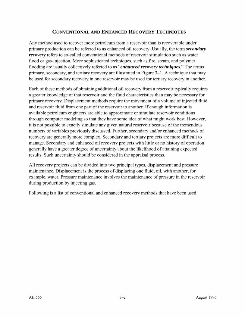
Any method used to recover more petroleum from a reservoir than is recoverable under primary production can be referred to as enhanced oil recovery. Usually, the term secondary recovery refers to so-called conventional methods of reservoir stimulation such as water flood or gas-injection. More sophisticated techniques, such as fire, steam, and polymer flooding are usually collectively referred to as “enhanced recovery techniques.” The terms primary, secondary, and tertiary recovery are illustrated in Figure 3–1. A technique that may be used for secondary recovery in one reservoir may be used for tertiary recovery in another.

Each of these methods of obtaining additional oil recovery from a reservoir typically requires a greater knowledge of that reservoir and the fluid characteristics than may be necessary for primary recovery. Displacement methods require the movement of a volume of injected fluid and reservoir fluid from one part of the reservoir to another. If enough information is available petroleum engineers are able to approximate or simulate reservoir conditions through computer modeling so that they have some idea of what might work best. However, it is not possible to exactly simulate any given natural reservoir because of the tremendous numbers of variables previously discussed. Further, secondary and/or enhanced methods of recovery are generally more complex. Secondary and tertiary projects are more difficult to manage. Secondary and enhanced oil recovery projects with little or no history of operation generally have a greater degree of uncertainty about the likelihood of attaining expected results. Such uncertainty should be considered in the appraisal process.

All recovery projects can be divided into two principal types, displacement and pressure maintenance. Displacement is the process of displacing one fluid, oil, with another, for example, water. Pressure maintenance involves the maintenance of pressure in the reservoir during production by injecting gas.

Following is a list of conventional and enhanced recovery methods that have been used.

AH 566 3–3 August 1996

Table 3–2 Recovery Methods

Conventional Recovery Methods Enhanced Recovery Methods

Water flooding Thermal (forward, reverse, and wet combustion fire flood, steam flood, and cyclic steam flood)

Gas injection Polymer flooding

Surfactant flooding

Microemulsion and micellar flooding

Carbon dioxide displacement

High pressure gas drive

Enriched-gas drive

Nitrogen, inert, and flue-gas injection

Economics always plays a prime role in the use of any recovery mechanism. Enhanced recovery techniques employed in California include waterflooding, steam drive, cyclic steam, and hot water drive. Engineers must take into consideration the economic availability of materials available to them to begin a recovery project after primary production. Even water may not be economically available.

WATERFLOODING Waterflooding is the oldest recovery method used, after primary recovery, and was discovered by accident when it was noted that there was increased oil production following an accidental flooding through abandoned wells in the Pithole City, Pennsylvania area in the late 1870’s. Today it is considered a reliable and economic approach to increase the percentage of recovery. Nearly every major field nearing depletion that does not have a natural water drive either has or is being considered for waterflooding.

Waterflooding is a conventional method in which water is injected into the reservoir and forces the movement of crude oil to nearby wells. It may be done on the periphery of the field or in an alternating injector and producer well configuration using converted oil wells or wells drilled for flood purposes. Premature breakthrough of a water front can result in a reduction of recoverable reserves. This is also a problem in any other type of flood displacement process. Careful management of the flood is needed to reduce the possibility of early breakthrough.

AH 566 3–4 August 1996

GAS INJECTION Gas injection is another conventional method of increasing oil recovery beyond primary production methods. It is used to maintain reservoir pressure at some level or to supplement natural reservoir pressures by the reinjection of produced gases, and it can result in improved hydrocarbon recoveries. Although not applicable in every field, it is important in fields containing volatile high-shrinkage crude oils or in gas-cap reservoirs with large quantities of retrograde condensate gas (gas that reverts to a liquid due to a reduction in reservoir pressure). It may also be used to prevent the oil from migrating into the gas cap in reservoirs where there is natural water drive or water injection down dip, as on the limb of a syncline. Oil gravity is important in fields employing gas injection, and recoveries increase as the viscosity of the oil approaches the viscosity of the displacing gas.

THERMAL There are basically two general types of thermal recovery, steam flood (continuous and cyclic) and fire flood (sometimes called in-situ combustion, both forward and reverse), both of which are enhanced recovery methods found in the southern San Joaquin Valley.

In steam flooding, which often follows cyclic steaming, steam is continuously injected into one well or a group of wells, while oil is produced from a different well or group of wells, similar to a conventional water-flood operation. In some case, cyclic steaming can be used in conjunction with a steam flood.

In cyclic steam flooding (also known as steam soak, intermittent steam injection, steam stimulation, and huff ‘n puff), steam is injected for a period of time such as a few days or weeks. The injecting well is then shut down for a period of time, and then reactivated as a producer. The amount of time used in the cycle is reservoir dependent. Cyclic steaming requires that there be sufficient remaining reservoir energy to cause oil to be produced.

Another thermal recovery method, under certain circumstances, is hot waterflooding. Instead of injecting steam, water below the boiling temperature is injected in much the same way as a regular waterflood. The heat is transferred to the oil and reduces the viscosity, allowing it to flow to production wells. Hot water is typically injected into a formation after the zone has already been steam flooded, but this is not a requirement.

Fire flooding is a recovery method where air is injected into the oil reservoir and the crude oil is ignited. The burning front advances by the continued injection of air. The heat generated reduces the viscosity of the oil, allowing it to flow more easily ahead of the burn front. Table 3–3 shows the three variations.

AH 566 3–5 August 1996

Table 3–3 Fire Flood Methods

Forward combustion Air is injected into a single well and the front moves away from the well into surrounding production wells.

Reverse combustion A burning front is begun at what will eventually be the producing well by the injection of air into it. The air flow is then moved to the adjacent wells and remains there. This process is especially suitable for very viscous oils that would not move through the cold zone in forward combustion.

Wet combustion A modified form of forward combustion with the additional factor of injecting cold water in order to help recover some of the heat between the air injection well and the burning front.

POLYMER FLOODING Polymer flooding is an enhanced recovery process that uses polysaccharides or polyacrylamides, which are large organic molecules. These molecular chains plug the more permeable channels in a formation. As water is injected into the formation, it is forced into the less permeable channels and displaces the oil there.

SURFACTANT FLOODING Petroleum sulfonates are used to reduce the interfacial tension between the oil and rock, thereby easing the flow of oil through the rock pores.

MICROEMULSION AND MICELLAR FLOODING Micellar flooding may recover all crude that it comes in contact with because the addition of a certain kind of surfactant creates a micro-emulsion of very small particle size. The tiny oil particles become entrapped in the center of the “micells” allowing easier movement through the reservoir.

CARBON DIOXIDE FLOODING Carbon dioxide will dissolve in oil creating miscibility, a single phase state under pressure, thus enhancing recovery. Alternatively, it can be dissolved in water and injected as carbonated water. The gas itself can also be injected alone, as a slug, to force the movement of oil. Basically, these three methods of carbon dioxide flooding depend on the type of crude, reservoir conditions, and economics.

HIGH PRESSURE GAS DRIVE Gas is injected at a pressure great enough to cause miscibility with the light fractions of oil. The enrichment of the gas with the light oil fractions causes its miscibility with the oil in the reservoir, thus enhancing production.

AH 566 3–6 August 1996

ENRICHED GAS DRIVE Prior to injection of the gas, it is enriched with light fractions. Upon injection, the light fractions in the gas condense and mix with the oil, thereby reducing its viscosity and becoming miscible with the oil.

NITROGEN, INERT, AND FLUE-GAS INJECTION This mechanism simply uses the injection of these gases for either the miscible or immiscible displacement of the oil.

AH 566 3–7 August 1996

Figure 3–1 Summary Of Recovery Methods and Their Relationship to Field Development

Natural Flow Artificial Lift

Pump Gas Lift Other

Secondary recovery

Waterflood

Tertiary recovery

PressureMaintenance

Water Dry HydrocarbonGas Injection

Thermal

CombustionSteam Soak/Cyclic/

Huff and PuffSteam drive/floodHot Water DriveElectromagnetic

Gasmiscible/

immiscible

HydrocarbonCO2

NitrogenFlue Gas

Chemical

AlkalinePolymer

Micellar/polymerFoam

Other

Microbial

EOR Recovery Mechanisms

Primary Recovery

Redrawn from OGJ April 20,1992, p. 5

En hanc ed oil rec overy

Con ven tion al Oil Rec overy

AH 566 4–1 August 1996

Chapter 4 : ESTIMATION OF RESERVES AND FUTURE PERFORMANCE

IMPORTANCE OF RESERVE ESTIMATES

The major asset of a petroleum property is its reserves. “Proved reserves,” as defined in Rule 468 (b), have a present economic value that is assessable for property tax purposes. Accurate predictions of reserves and future production schedules are the most important part of a petroleum appraisal and may be difficult to accomplish. Reserves are only estimated volumes of what recovery could be if the assumptions made are accurate and factual. The point at which recovery can be determined with absolute certainty is after the well has been abandoned.

Estimates of reserves are dependent on a number of factors, the most important of which are recovery method and economics. Reserve estimates are dynamic, changing often throughout the life of the field. The first question any appraiser should ask when looking at a reserves estimate is what technical and economic assumptions are associated with the forecast. Without knowing the economic assumptions, the reserve estimate is nearly useless. Estimates of recoverable petroleum that do not consider the economics of production are best described as technical reserves. Although it is generally accepted that all of the oil and gas existing but not yet recovered is in place, no one can accurately estimate the extent of such deposits. (See Lynch v. State Bd. of Equalization, (1983) 164 Cal.App.3d 94.) Even though under current or expected development of the property, technical reserves could be produced, whether or not they will be produced depends entirely upon future economic conditions.

DEFINITION OF RESERVES

PROVED RESERVES There is only one definition of proved reserves, however, that is authoritative for property tax appraisal purposes in California. That definition is found in Rule 468(b), which describes “proved reserves” as:

“…those reserves which geological and engineering information indicate with reasonable certainty to be recoverable in the future, taking into account reasonably projected physical and economic operating conditions. Present and projected economic conditions shall be determined by reference to all economic factors considered by knowledgeable and informed persons engaged in the operation and buying or selling of such properties, e.g., capitalization rates, product prices and operation expenses.”

In this definition, future expectations about prices and expenses are specifically considered, because in determining market value, operators, sellers, and purchasers will carefully

AH 566 4–2 August 1996

consider the variation of product prices from their current levels in order to determine the effect on the profitability of the property. The significant difference between the Rule definition of proved reserves and the SPE or SPEE definition is that Rule 468(b) allows inclusion of reserves derived from future expectations for product prices and operating costs. Rule 468 authorizes subtraction from taxable value for deletions in proved reserves and increases in the taxable value of the petroleum property where there are additions to proved reserves. A history and analysis of this definition of proved reserves is further explained in Lynch v. State Bd. of Equalization, p.105.

There are numerous other definitions for “proved reserves.” The Securities Exchange Commission has a definition designed for investors making annual economic comparisons among companies. The Society of Petroleum Engineers (SPE) defines “proved reserves” as volumes that “…can be estimated with reasonable certainty to be recovered under current economic conditions.” “Reasonable certainty” in this context means that a reservoir is proved if the area is delineated by drilling, defined by fluid contacts, and the undrilled areas can be reasonably judged to be commercially productive on the basis of available geologic and engineering data. Proved reserves must have facilities to process and transport those reserves to market that are operational at the time of the estimate, or there is a commitment or reasonable expectation to install such facilities in the future.1 In the case of enhanced recovery methods, reserves can be considered proved upon completion of a successful pilot study, or a favorable response from an enhanced recovery program in the specific reservoir or one in the immediate area with similar rock and fluid properties.

The Society of Petroleum Evaluation Engineers (SPEE) maintains, as does the SPE, that “proved reserves” do not include reserves that are the result of projected increases in prices. This element also requires that proved undeveloped reserves be restricted to immediate offset locations in geologic formations that have demonstrated economic productivity, and that the offset locations conform to existing well spacing regulations. In the SPEE definition, reserves attributed to enhanced recovery are restricted to successful pilot testing or favorable production response in the specific reservoir or within the immediate area with similar rock and fluid properties.

Within the SPE/SPEE classification of proved reserves there are three subclasses. They are Proved Developed Reserves, Proved Developed Nonproducing Reserves, and Proved Undeveloped Reserves. These are all taxable under Rule 468.

Proved developed reserves refer to estimates of reserves that can be recovered from existing completion intervals and production facilities. Developed reserves may require additional expenditures such as the installation of artificial lift or gas compression. The implication is that the equipment and operating practices are well known and the equipment needed is commercially available, i.e., does not require significant new design and fabrication efforts.

1 Monograph I, The Society of Petroleum Evaluation Engineers, Guidelines for the Application of the Definition For Oil and Gas Reserves, December 1988, p. 3

AH 566 4–3 August 1996

Proved developed nonproducing reserves are reserves estimates where the production is shutin. This would include behind-pipe reserves for wells with multiple pay zones or well shutin pending some other action such as completion of a pipeline of production facility, repair of a mechanical problem, or waiting on a stimulation treatment.

The classification of proved undeveloped reserves is assigned to estimates of reserves for undrilled, offset locations or deeper productive zones in an existing well. These reserves are considered proved if geological, geophysical, and engineering information support the interpretation that the location will be productive. Only reserves as defined by Rule 468(b) are subject to assessment.

METHODS

There are five general methods of predicting future recovery from a reservoir. Each depends upon different types of information and varies in its accuracy based on the input data and the age of the field development. The methods are:

• Analogy

• Volumetric

• Material Balance

• Decline Curves

• Reservoir Simulation.

Each method requires different data, and the various results should be compared in order to test assumptions about the reservoir. It is possible to reconcile the differences between various reserve estimates in the same way different appraisal methods are reconciled to arrive at fair market value. Figure 4–1, at the end of this discussion, shows the relationship between the different methods, the relative range, and the relative risk of the estimates. This figure assumes the continuation of a single recovery method. The introduction of a new recovery method will often necessitate the reversion back to a higher relative risk.

ANALOGY Reserve estimation by analogy attempts to compare one property or well with another to gain an insight into its potential. Estimates by analogy are typically made when little information is known about the reservoir and production capabilities. Comparisons are made with properties that have similar geological characteristics and reservoir conditions. These can either be offset wells, offset properties, or information from the same zone in other fields.

The difficulty of reserve estimation by analogy is determining that two reservoirs are comparable. Often barrels per acre–foot, or barrels per acre, are used as units of comparison. This assumes that the other reservoir properties between the subject field and the analogous field are similar. Reservoir development and positioning are critical factors in determining

AH 566 4–4 August 1996

the comparability of properties. Since oil and gas are lighter than water, properties positioned higher on the geologic structure will have better production characteristics. Reserve estimation by analogy is viewed as the least accurate of the methods presented.

Analogy can be used as a reserve estimation technique during all phases of a properties status from predrilling through development. The accuracy of analogy methods is highly dependent on the data used.

“The analogy method should be applied as a check for reasonableness even when other methods have been utilized for estimating reserves. It is recognized that analogies will be imperfect, and the reserve estimator may adjust historical performance data using theoretical methods.”2

VOLUMETRIC Volumetric reserve estimates can be made early in the life of a project or well. The volumetric method estimates the available pore space in the reservoir, the portion containing hydrocarbons, and how much of the resource can be removed. At a minimum, estimates are required about the aerial extent (A), height (h), porosity (φ), and water saturation (Sw). Much of this information is available from well logs, core analysis, or other geological information. The accuracy of the reserve estimate is related to the accuracy of the input data. This method is often used to determine whether additional funds will be spent to complete the well.

The formation oil factor (Boi) and the formation gas factor (Bgi) are used to convert the estimates at the temperature and pressure below the surface into surface and sales volumes. The values for Boi and Bgi are determined by laboratory analysis or from correlation tables.

For Oil Reserves = 7758 1Ah SB

RFw

oi

φ ( )− Equation 4–1

For Gas Reserves = 43560 1Ah SB

RFw

gi

φ ( )− Equation 4–2

Volumetric reserves can be estimated for either a single well or the entire field. The constants in the equations represent the number of barrels in one acre-foot and the number of cubic feet per acre-foot respectively.

The reserve estimate generated by volumetric methods is the original oil or gas in place. A recovery factor (RF) is needed to arrive at proved reserves. The recovery factor is a function of several separate efficiencies affected by the geology of the reservoir, rock and fluid characteristics, and the well density. Recovery factors can range anywhere from 5 percent to

2 Ibid., p.11

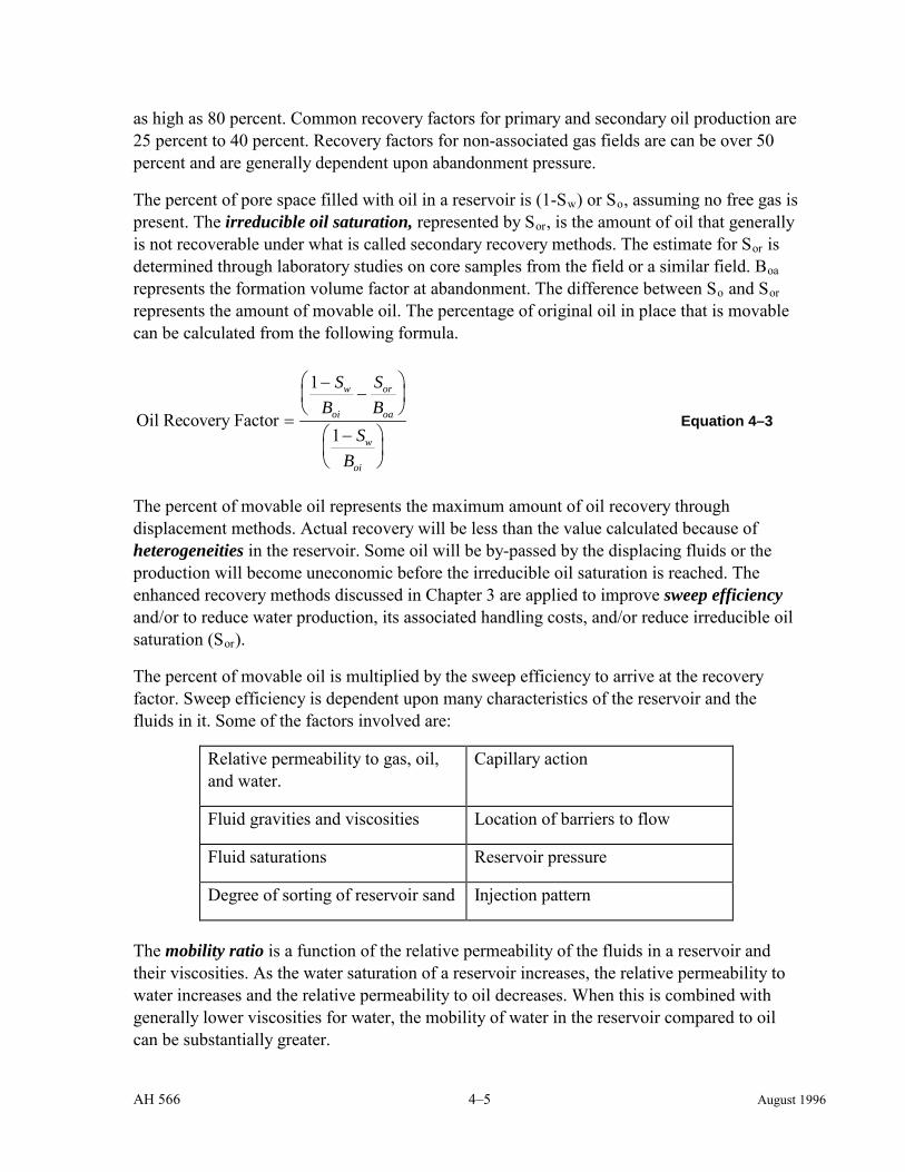
AH 566 4–5 August 1996

as high as 80 percent. Common recovery factors for primary and secondary oil production are 25 percent to 40 percent. Recovery factors for non-associated gas fields are can be over 50 percent and are generally dependent upon abandonment pressure.

The percent of pore space filled with oil in a reservoir is (1-Sw) or So, assuming no free gas is present. The irreducible oil saturation, represented by Sor, is the amount of oil that generally is not recoverable under what is called secondary recovery methods. The estimate for Sor is determined through laboratory studies on core samples from the field or a similar field. Boa represents the formation volume factor at abandonment. The difference between So and Sor represents the amount of movable oil. The percentage of original oil in place that is movable can be calculated from the following formula.

Oil Recovery Factor =

−−

−

1

1

SB

SB

SB

w

oi

or

oa

w

oi

Equation 4–3

The percent of movable oil represents the maximum amount of oil recovery through displacement methods. Actual recovery will be less than the value calculated because of heterogeneities in the reservoir. Some oil will be by-passed by the displacing fluids or the production will become uneconomic before the irreducible oil saturation is reached. The enhanced recovery methods discussed in Chapter 3 are applied to improve sweep efficiency and/or to reduce water production, its associated handling costs, and/or reduce irreducible oil saturation (Sor).

The percent of movable oil is multiplied by the sweep efficiency to arrive at the recovery factor. Sweep efficiency is dependent upon many characteristics of the reservoir and the fluids in it. Some of the factors involved are:

Relative permeability to gas, oil, and water.

Capillary action

Fluid gravities and viscosities Location of barriers to flow

Fluid saturations Reservoir pressure

Degree of sorting of reservoir sand Injection pattern

The mobility ratio is a function of the relative permeability of the fluids in a reservoir and their viscosities. As the water saturation of a reservoir increases, the relative permeability to water increases and the relative permeability to oil decreases. When this is combined with generally lower viscosities for water, the mobility of water in the reservoir compared to oil can be substantially greater.

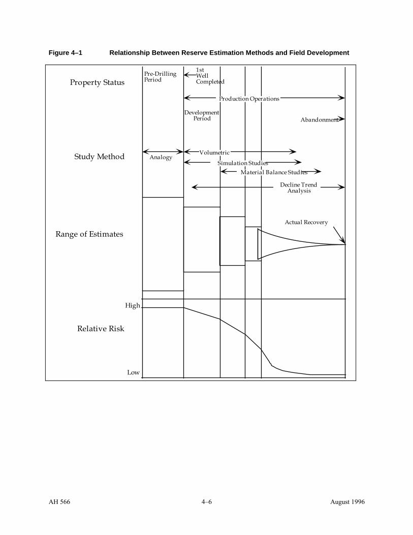
AH 566 4–6 August 1996

Figure 4–1 Relationship Between Reserve Estimation Methods and Field Development

Property Status

Study Method

Range of Estimates

Relative Risk

High

Low

Pre-DrillingPeriod

1stWellCompleted

Production Operations

DevelopmentPeriod Abandonment

AnalogyVolumetric

Simulation StudiesMaterial Balance Studies

Actual Recovery

Decline TrendAnalysis

AH 566 4–7 August 1996

Example 4–1 Volumetric Estimation of Oil Reserves

Given:

A = 640 acres Sw = 35%

φ = 13% Boi = 1.1 Reservoir barrels/Stock Tank barrel

h = 15 ft Sor = 0.2

Reserves

Bbls

=− − −

−

=

7758 640 15 13 1 3511

1 2 351 35

3 812

( )( )(. )( . ).

. ..

,960,

Example 4–2 Volumetric Estimation of Gas Reserves

Given:

A = 1920 acres Sw = 20%

φ = 25% Bgi = 1.04 cubic feet/standard cubic feet

h = 35 ft Sga = 20%

Reserves

MMCF

=− − −

−

=

43560 1920 35 25 1 2104

1 2 21 2

422

( )( )(. )( . ).

. ..

PERFORMANCE ANALYSIS Several methods of predicting reserves rely on measuring the past performance and extrapolating this into the future. Performance analysis methods of reserve estimation include: material balance calculations, decline or performance curve analysis, and reservoir simulation models.

Material Balance The material balance approach to estimate reserves is based on the principle of the conservation of mass. The mass or volume produced is equal to the mass or volume originally in place less the mass or volume currently in place. The complexity of most material balance equations makes them of limited use without training in reservoir engineering.

AH 566 4–8 August 1996

Material balance equations are applied to the reservoir as if it were a “tank.” Inflows and outflows are measured against successive declines in pressure. Graphical material balance methods are widely used for dry gas reservoirs. One basic assumption is that there is no water influx into the reservoir. Input requirements are limited to reservoir pressure, gas gravity, and production. A plot of pressure divided by the real gas deviation factor (Z) versus the cumulative production is made, the trend extrapolated, and recoverable reserves read at the abandonment pressure.

Performance or Decline Curves Decline curves represent one of the most useful tools for the petroleum property appraiser when dealing with properties, where sufficient data are available to allow a reasonable extrapolation for obtaining an estimate of future production. They require no assumptions about reservoir parameters and are based entirely on the past performance of the specific property. The difficulty with decline curves is that they are deceptively simple. Proper analysis of decline curves involves more than drawing a line through points on a graph. Variations on the production plot need to be highlighted and, if possible, explained. If problems develop in the reservoir, the result will be indicated on the production curve. Evaluation of the reservoir will determine whether the problem can be corrected or a new trend has been established.

Types of Curves The inherent assumption in decline curve analysis is that the factors that affected the production in the past will continue to do so in the future. There are six common types of production curves, as follows:

• Production Rate versus Time

• Production Rate versus Cumulative Production

• Percentage Water Cut in Production versus Cumulative Production

• Water Level versus Cumulative Production

• Cumulative Gas Produced versus Cumulative Oil

• Pressure versus Cumulative Production

Depending on the production history available for the property and its current operating conditions, different curves will prove more useful than others in predicting future performance. The common feature and assumption of all decline curves is that once a trend has been established, it should continue, although more production does not ensure that the estimator will predict the remaining reserves with improved accuracy.

Fields with an active water drive will find utility using the Water Level versus Cumulative Production curve. A line is drawn on a graph representing the top of the producing formation and as the water level increases, displacing petroleum, the cumulative production is plotted.

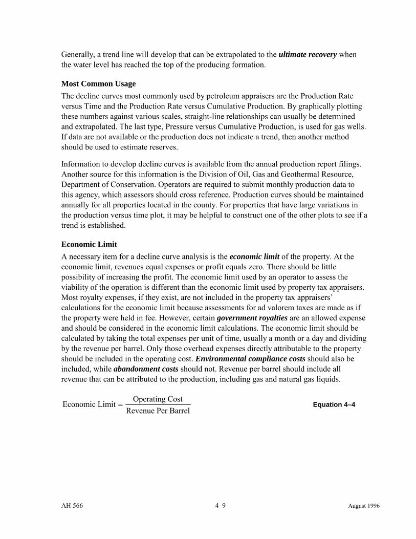
AH 566 4–9 August 1996

Generally, a trend line will develop that can be extrapolated to the ultimate recovery when the water level has reached the top of the producing formation.

Most Common Usage The decline curves most commonly used by petroleum appraisers are the Production Rate versus Time and the Production Rate versus Cumulative Production. By graphically plotting these numbers against various scales, straight-line relationships can usually be determined and extrapolated. The last type, Pressure versus Cumulative Production, is used for gas wells. If data are not available or the production does not indicate a trend, then another method should be used to estimate reserves.

Information to develop decline curves is available from the annual production report filings. Another source for this information is the Division of Oil, Gas and Geothermal Resource, Department of Conservation. Operators are required to submit monthly production data to this agency, which assessors should cross reference. Production curves should be maintained annually for all properties located in the county. For properties that have large variations in the production versus time plot, it may be helpful to construct one of the other plots to see if a trend is established.

Economic Limit A necessary item for a decline curve analysis is the economic limit of the property. At the economic limit, revenues equal expenses or profit equals zero. There should be little possibility of increasing the profit. The economic limit used by an operator to assess the viability of the operation is different than the economic limit used by property tax appraisers. Most royalty expenses, if they exist, are not included in the property tax appraisers’ calculations for the economic limit because assessments for ad valorem taxes are made as if the property were held in fee. However, certain government royalties are an allowed expense and should be considered in the economic limit calculations. The economic limit should be calculated by taking the total expenses per unit of time, usually a month or a day and dividing by the revenue per barrel. Only those overhead expenses directly attributable to the property should be included in the operating cost. Environmental compliance costs should also be included, while abandonment costs should not. Revenue per barrel should include all revenue that can be attributed to the production, including gas and natural gas liquids.

Economic Limit Operating CostRevenue Per Barrel

= Equation 4–4

AH 566 4–10 August 1996

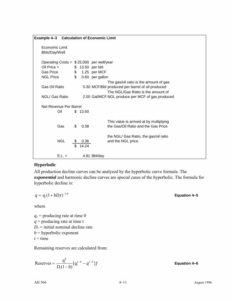
AH 566 4–11 August 1996

Hyperbolic All production decline curves can be analyzed by the hyperbolic curve formula. The exponential and harmonic decline curves are special cases of the hyperbolic. The formula for hyperbolic decline is:

q q bD ti ib= + −( ) /1 1 Equation 4–5

where

qi = producing rate at time 0 q = producing rate at time t Di = initial nominal decline rate b = hyperbolic exponent t = time

Remaining reserves are calculated from:

Reserves =−

−− −qD b

q q fib

ii

b b

( )[ ]

11 1 Equation 4–6

Example 4–3 Calculation of Economic Limit

Economic LimitBbls/Day/Well

Operating Costs = 25,000$ per well/yearOil Price = 13.50$ per bblGas Price 1.25$ per MCFNGL Price 0.60$ per gallon

Gas Oil Ratio 0.30 MCF/BblThe gas/oil ratio is the amount of gas produced per barrel of oil produced

NGL/ Gas Ratio 2.00 Gal/MCFThe NGL/Gas Ratio is the amount of NGL produce per MCF of gas produced

Net Revenue Per BarrelOil 13.50$

Gas 0.38$ This value is arrived at by multiplying the Gas/Oil Ratio and the Gas Price

NGL 0.36$

y y g the NGL/ Gas Ratio, the gas/oil ratio and the NGL price.

14.24$

E.L. = 4.81 Bbl/day

AH 566 4–12 August 1996

where qi = producing rate at time 0 q = producing rate at time t, the economic limit Di = the initial decline rate b = hyperbolic constant f = time adjustment factor

The time adjustment factor is used to cancel out the time units in the equation and its value is dependent upon the time units for q and D. If q is in barrels per day and D is the rate per year, then f is equal to 365.

Hyperbolic decline of a production stream may become more apparent later in the life of a property. The production decline will begin to flatten out, effectively extending the life of the property.

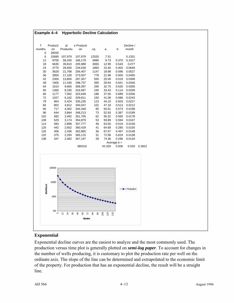
AH 566 4–13 August 1996

Exponential Exponential decline curves are the easiest to analyze and the most commonly used. The production versus time plot is generally plotted on semi-log paper. To account for changes in the number of wells producing, it is customary to plot the production rate per well on the ordinate axis. The slope of the line can be determined and extrapolated to the economic limit of the property. For production that has an exponential decline, the result will be a straight line.

Example 4–4 Hyperbolic Decline Calculation

T months

Production

al Productio

e Production ∆q a b

Decline / month

0 282006 15680 107,979 107,979 12520 7.51 0.1331

12 9700 58,200 166,179 5980 9.73 0.370 0.102718 6635 39,810 205,989 3065 12.99 0.543 0.07724 4775 28,650 234,639 1860 15.40 0.402 0.064930 3628 21,768 256,407 1147 18.98 0.596 0.052736 2850 17,100 273,507 778 21.98 0.500 0.045542 2300 13,800 287,307 550 25.09 0.519 0.039948 1905 11,430 298,737 395 28.94 0.641 0.034654 1610 9,660 308,397 295 32.75 0.635 0.030560 1365 8,190 316,587 245 33.43 0.114 0.029966 1177 7,062 323,649 188 37.56 0.689 0.026672 1027 6,162 329,811 150 41.08 0.586 0.024378 904 5,424 335,235 123 44.10 0.503 0.022784 802 4,812 340,047 102 47.18 0.513 0.021290 717 4,302 344,349 85 50.61 0.573 0.019896 644 3,864 348,213 73 52.93 0.387 0.0189

102 582 3,492 351,705 62 56.32 0.565 0.0178108 529 3,174 354,879 53 59.89 0.594 0.0167114 483 2,898 357,777 46 63.00 0.519 0.0159120 442 2,652 360,429 41 64.68 0.280 0.0155126 406 2,436 362,865 36 67.67 0.497 0.0148132 375 2,250 365,115 31 72.58 0.819 0.0138138 347 2,082 367,197 28 74.36 0.296 0.0134

Average b = 380316 42.329 0.506 0.033 0.3922

100

1000

10000

100000

0 12 24 36 48 60 72 84 96 108

120

132

Months

Bbl

/Mon

th

Production

AH 566 4–14 August 1996

As mentioned above, the exponential decline formulas are a special case of the hyperbolic decline. A hyperbolic exponent of zero indicates exponential decline. The equation for a straight line on semi-log paper is:

q q eiDt= − Equation 4–7

where q = producing rate at time t qi = producing rate at time 0 D = nominal exponential decline rate per unit of time t= time e = base of natural logarithms

Reserves are calculated from

Reserves = −q qD

fi Equation 4–8

The following example illustrates the procedure.

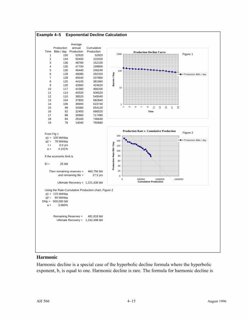
AH 566 4–15 August 1996

Harmonic Harmonic decline is a special case of the hyperbolic decline formula where the hyperbolic exponent, b, is equal to one. Harmonic decline is rare. The formula for harmonic decline is

Example 4–5 Exponential Decline Calculation

TimeProduction Bbls / day

Average annual

ProductionCumulative Production

Production Bbls

/ day1 150 52920 52920 1502 144 50400 103320 1443 136 48780 152100 1364 135 47700 199800 1355 130 46440 246240 1306 128 46080 292320 1287 128 45540 337860 1288 125 44100 381960 1259 120 42660 424620 120

10 117 41580 466200 11711 114 40320 506520 11412 110 38520 545040 11013 104 37800 582840 10414 106 36900 619740 10615 99 34380 654120 9916 92 32400 686520 9217 88 30960 717480 8818 84 29160 746640 8419 78 14040 760680 78

From Fig 1q1 = 100 bbl/dayq2 = 78 bbl/day

t = 6.0 yrsa = 4.141%

If the economic limit is

El = 25 bbl

Then remaining reserves = 460,756 bbland remaining life = 27.5 yrs

Ultimate Recovery = 1,221,436 bbl

Using the Rate-Cumulative Production chart, Figure 2q1 = 115 bbl/dayq2 = 60 bbl/day

DNp = 500,000 bbla = 3.960%

Remaining Reserves = 481,818 bblUltimate Recovery = 1,242,498 bbl

Production Decline Curve

1

10

100

1000

1 3 5 7 9 11 13 15 17 19

TimeB

arre

ls /

Day Production Bbls / day

Figure 1

Production Rate v. Cumulative Production

0

20

40

60

80

100

120

140

160

0 500000 1000000 1500000Cumulative Production

Prod

uctio

n R

ate

Bbl

/ D

ay

Production Bbls / day

Figure 2

AH 566 4–16 August 1996

q qD ti

i

=+1

Equation 4–9

and for reserves

Reserves = qD

qq

fi

i

iln Equation 4–10

Since fluctuations in the production rate may make it difficult to interpret the data when plotted on a monthly basis, it is sometimes helpful to average production over 3–month, 6–month, or 1–year periods.

Reservoir Simulation Reservoir simulation uses computer models to predict reserves and production schedules. Simulations typically require a great deal of information and are not typically done in a property tax appraisal. A reservoir simulation breaks down the reservoir into many small interconnected blocks. The model projects fluid flow across the boundaries of the blocks. For each block in the simulation, values for porosity, permeability, pressure, fluid saturation, and other information must be determined. The accuracy of the model is measured by making a history match against past production. Once the history match is made, the predictive phase of the simulation can start.

While reservoir simulations can appear very impressive, they should be viewed with caution. The output of the simulation is only as reliable as the data inputs. It is very easy to manipulate the data to arrive at a desired result. If a simulation is presented for inclusion in an appraisal, the appraiser should examine why the simulation was constructed and whether the assumptions in the simulation are appropriate. In subsequent years, the output of the simulation should be tracked against the actual production, and any deviations should be satisfactorily explained.

FUTURE PERFORMANCE

Future performance for any well or field can only be estimated. Reliability of these predictions will be subject to the accuracy of the data used and assumptions made. Future performance predictions are generally made from data used in either the material balance equations or from production decline curve data. The discussion contained herein is restricted to performance predictions based on decline curve analysis.

FORECASTING PRODUCTION A realistic approach when forecasting production properly accounts for downtime associated with equipment failure and maintenance. Since no equipment can operate continuously, reasonable periods of downtime should be forecast to allow for maintenance and repair.

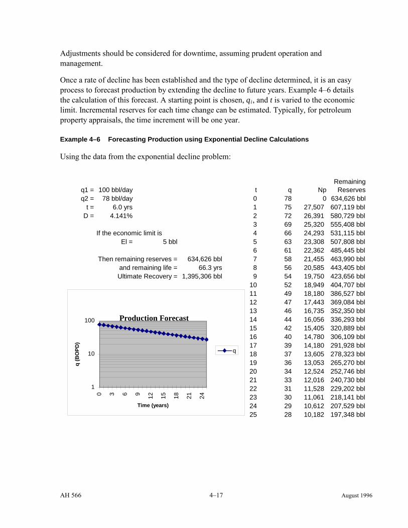
AH 566 4–17 August 1996

Adjustments should be considered for downtime, assuming prudent operation and management.

Once a rate of decline has been established and the type of decline determined, it is an easy process to forecast production by extending the decline to future years. Example 4–6 details the calculation of this forecast. A starting point is chosen, qi, and t is varied to the economic limit. Incremental reserves for each time change can be estimated. Typically, for petroleum property appraisals, the time increment will be one year.

Example 4–6 Forecasting Production using Exponential Decline Calculations

Using the data from the exponential decline problem:

q1 = 100 bbl/day t q NpRemaining Reserves

q2 = 78 bbl/day 0 78 0 634,626 bblt = 6.0 yrs 1 75 27,507 607,119 bbl

D = 4.141% 2 72 26,391 580,729 bbl3 69 25,320 555,408 bbl

If the economic limit is 4 66 24,293 531,115 bblEl = 5 bbl 5 63 23,308 507,808 bbl

6 61 22,362 485,445 bblThen remaining reserves = 634,626 bbl 7 58 21,455 463,990 bbl

and remaining life = 66.3 yrs 8 56 20,585 443,405 bblUltimate Recovery = 1,395,306 bbl 9 54 19,750 423,656 bbl

10 52 18,949 404,707 bbl11 49 18,180 386,527 bbl12 47 17,443 369,084 bbl13 46 16,735 352,350 bbl14 44 16,056 336,293 bbl15 42 15,405 320,889 bbl16 40 14,780 306,109 bbl17 39 14,180 291,928 bbl18 37 13,605 278,323 bbl19 36 13,053 265,270 bbl20 34 12,524 252,746 bbl21 33 12,016 240,730 bbl22 31 11,528 229,202 bbl23 30 11,061 218,141 bbl24 29 10,612 207,529 bbl25 28 10,182 197,348 bbl

Production Forecast

1

10

100

0 3 6 9 12 15 18 21 24

Time (years)

q (B

OPD

)

q

AH 566 5–1 August 1996

Chapter 5 : GENERAL APPRAISAL METHODS AND ASSESSMENT UNDER PROPOSITION 13

INTRODUCTION

While petroleum-producing properties differ in important ways from other real property, they nonetheless lend themselves to appraisal through the traditionally recognized cost, income, and market approaches to value. The purpose of this chapter is to review briefly the essentials of these traditional methods of determining market value and the impact of Proposition 13 on petroleum-producing properties.

“VALUE” FOR PURPOSES OF PROPERTY TAXATION For purposes of property taxation, “value” is determined by Sections 110 and 110.1 of the Revenue and Taxation Code1 and Rule 2.

Section 110 defines value as follows:

“Except as is otherwise provided in Section 110.1, ‘full cash value’ or ‘fair market value’ means the amount of cash or its equivalent which property would bring if exposed for sale in the open market under conditions in which neither buyer nor seller could take advantage of the exigencies of the other and both with knowledge of all the uses and purposes to which the property is adapted and for which it is capable of being used and of the enforceable restrictions upon those uses and purposes.”

Section 110.1 defines value as follows:

“(a) For purposes of subdivision (a) of Section 2 of Article XIII A of the California Constitution, ‘full cash value’ of real property, including possessory interests of real property, means the fair market value as determined pursuant to Section 110 for either:

(1) The 1975 lien date; or,

(2) For property which is purchased, is newly constructed or changes ownership after the 1975 lien date:

(A) The date on which a purchase or change in ownership occurs; or

(B) The date on which new construction is completed, and if uncompleted, on the lien date.

1 All statutory references are to the Revenue and Taxation Code unless otherwise indicated.

AH 566 5–2 August 1996

(b) The value determined under subdivision (a) shall be known as the base year value for the property.”

Subsections (c) through (e) clarify the concept of “base year.” Subsection (f) limits the annual increase in the full cash value to 2 percent.

The Board has interpreted Section 110 in Property Tax Rule 2 which describes value in subdivision (a) as follows:

“In addition to the meaning ascribed to them in the Revenue and Taxation Code, the words ‘full value,’ ‘full cash value,’ ‘cash value,’ ‘actual value,’ and ‘fair market value’ mean the price at which a property, if exposed for sale in the open market with a reasonable time for the seller to find a purchaser, would transfer for cash or its equivalent under prevailing market conditions between parties who have knowledge of the uses to which the property may be put, both seeking to maximize their gains and neither being in a position to take advantage of the exigencies of the other.

“When applied to real property, the words ‘full value’, ‘full cash value’, ‘cash value’, ‘actual value’ and ‘fair market value’ mean the prices at which the unencumbered or unrestricted fee simple interest in the real property (subject to any legally enforceable government restrictions) would transfer for cash or its equivalent under the conditions set forth in the preceding sentence.”

THE APPRAISAL PROCESS Definition An appraisal is an opinion of value. In order to accurately and systematically arrive at such an opinion, a logical method of collecting, analyzing, and processing data must be developed in order to make a sound judgment of the value of a specific property.

Steps in the Appraisal Process

Define the Problem It is necessary to establish the kind of value that is being sought (e.g. market value), the appraisal unit, the rights being appraised (fee simple absolute, except for taxable possessory interests), and the date of the appraisal (the date of change in ownership or new construction if after March 1, 1975, or the lien date for appraisals where “Proposition 8” applies).

Conduct a Preliminary Survey The location of the subject property should be surveyed to determine the patterns of actual property use and its highest and best use.

AH 566 5–3 August 1996

Collect Data Any appraisal method requires the collection and verification of data by appraisers. This data should include documentary transfer tax, change in ownership statements, construction contracts, lease data, and other kinds of information about the subject property.

Process the Data into Indicators of Value The appraiser must estimate the present worth of anticipated future net benefits through one or more of the three major methods of processing data into value indicators: the sales comparison, capitalized income, and cost approaches to value.

Data should be independently processed for each approach to value. No method of appraisal should be forced to agree with any other method. An important consideration is that each approach be objectively developed.

Reconcile the Indicators Reconciliation is not the arithmetic averaging of the various value indicators. It is the process of critically evaluating how well each indicator reflects the factors influencing the value of the subject property. The appraiser will weigh most heavily that indicator which best measures the type of benefits the subject property yields.

Draw a Value Conclusion This is the final step in the appraisal process, in which the appraiser presents a reasoned opinion supported by factual data that can be evaluated by an observer.

THE THREE APPROACHES TO VALUE

Property Tax Rule 3 prescribes the application of one or more of the following approaches to value in order to arrive at the “full cash value” mentioned in Rule 2: comparative sales approach, stock and debt approach, replacement/reproduction cost approach, historical cost approach, or income approach.

The first two are actually both sales comparison. In the stock and debt approach, the present value of all stock is added to the present value of all liabilities. The sale of shares of stock represents the sale of fractional interests in the property. If there were always an abundance of similar properties on the market, the sales comparison approach is always preferred. In the comparative sales approach, similar property sales are required.

The replacement, reproduction, and historical cost approaches are all variants of the cost approach. The income approach is the most used methodology in petroleum property appraisals.

AH 566 5–4 August 1996

THE COMPARATIVE SALES APPROACH Property Tax Rule 4 The comparative sales approach is any approach that relies on direct evidence of the market’s opinion of value of a property, preferably in the form of confirmed sales of similar properties.

In contrast to the cost and income approaches, the comparative sales approach offers direct rather than indirect evidence of market value. It is the preferred method when there are sufficient sales available to invite comparison with the subject property and to adjust the selling prices of the sold properties to make them truly comparable.

Property Tax Rule 4 prescribes the manner in which property tax appraisers must apply the comparative sales approach. Several conditions must be met:

(a) non-cash consideration (e.g., personal property) included in the transaction must be converted to its cash equivalent;

(b) seller-paid loan points charged by a lender must be deducted from the nominal sale price;

(c) assumed loans, promissory notes, or other “paper” consideration must be converted to its cash equivalent;

(d) the positive or negative value of a lease encumbering the property at the time of sale must be added to or subtracted from the selling price;

(e) the sale prices of comparable properties must be adjusted for any change in the price level of this type of property between the time the sale price was negotiated and the date of valuation of subject property; and

(f) make appropriate allowances for differences between the comparable properties at the time of sale and the subject property on the valuation date, as to physical attributes, location, enforceable restrictions upon use, and anticipated income and amenities.

Market Units of Comparison It is often helpful to the appraiser to express the adjusted selling prices of comparable sales in terms of a unit selling price that can readily be applied to subject property. For instance, bare land sales can be expressed in terms of selling price per square foot, front foot, or buildable site; single-family residential sales lend themselves to selling price per square foot of main living area; commercial property sales are commonly expressed as selling price per square foot of net rentable area or lineal foot of frontage; and sales of income-producing multiple-residential properties are commonly reduced to rent multipliers or selling price per bedroom. One typical denominator applied to oil wells is selling price per barrel of oil equivalent reserves.

AH 566 5–5 August 1996

The appraiser must judiciously select and adjust the comparable sales prices before converting them into convenient units of comparison.

Sale of Subject Property When valuing property as the result of a change in ownership, Section 110 (b) and Rule 2 (b) provide a rebuttable presumption that the amount of monetary consideration or its equivalent paid for real property sold is its “full cash value.” If the assessor chooses to rebut the presumption, he/she must do so by a “preponderance of the evidence” establishing that the consideration paid is not market value. This rebuttable presumption does not apply to transfers of taxable possessory interests, changes in control of legal entities through stock acquisition, or transfers of partnership interests, or any unreported transfers for which no change in ownership statement was timely filed. Rule 2 also requires that for transfers of more than one parcel, the purchase price must be allocated among the sold parcels in proportion to the relative fair market value of each.

Income Multipliers Income-producing properties may be compared on the basis of multiples of their gross or net incomes. Income multipliers, whether calculated at the level of gross or net operating income, are properly considered part of the market data approach (although Rule 8(h) states that income may be capitalized by using gross income, rent, or production multipliers). Income multipliers are factors rather than rates. The basic formula for a gross income multiplier (GIM) is:

GIM VI

= Equation 5–1

where V = cash equivalent selling price of a comparable property I = anticipated maximum earning capacity of sold property (Note: this may differ

from its actual income).

When appraising smaller residential properties, appraisers commonly speak of gross rent multipliers. The term, gross income multiplier, is more useful for larger apartment projects and commercial properties, since these types of properties frequently return additional income attributable to sources other than basic building rent, e.g., parking, laundry, or storage area.

To apply this useful tool to a subject property, the appraiser determines the multipliers from sold properties that are similar to the subject, selects a multiplier, and applies it to the economic income of the subject property. For example, if an apartment house comparable to the subject property sold for $500,000 and its potential gross income was $80,000 at the time

AH 566 5–6 August 1996

of sale, the gross income multiplier would be $500,000 / $80,000, or 6.25. This factor could be applied to the potential gross income of the subject to produce an indicator of market value.

Income multipliers must be derived from sales of very similar properties. “Similar” means alike in terms of use, remaining economic life, physical condition, land to building value ratio, and other characteristics. If a net income multiplier is sought, the appraiser must be sure that similar properties are used and the ratio of gross to net income is the same for both comparable sales and subject property. That is, the operating expense ratio should be similar. The unit of comparison selected must be consistently applied to the subject property and all comparable sales properties in each analysis. For additional information on the use of multipliers, the appraiser is referred to Assessors’ Handbook Section 501A.

THE COST APPROACH Property Tax Rule 6 prescribes how both reproduction and replacement costs shall be estimated. Subdivision (a) specifies in part that the cost approach is preferred when neither reliable sales nor income data are available. The cost approach provides a useful tool in the valuation of petroleum property improvements and personalty. It is also well adapted to construction in progress and property that is properly located and does not suffer from unusual amounts of obsolescence of any kind.

Replacement or Reproduction Cost Reproduction cost is the outlay required as of a certain date to replace an existing structure with an exact replica. This variant of the cost approach is of limited usefulness because it is frequently not possible or desirable to replace an existing structure, due either to the lack of certain materials or trade skills, or because of the functional obsolescence of the older structure.

Replacement cost is the cost required, as of a certain date, to replace an existing structure with one possessing equivalent utility. This concept is widely accepted in appraisal practice. The appraiser must estimate not only replacement cost new, but also the accrued depreciation in the structure, which is the most difficult aspect of applying the replacement or reproduction cost approaches.

For property tax appraisal purposes, depreciation is defined as the loss in value from any cause, and it is the measure of the loss in value experienced by a property compared to a hypothetical and similar property that has suffered no depreciation. Depreciation, in the appraisal sense, is the difference between the present market value of improvements and their replacement cost new. To estimate depreciation, appraisers commonly refer to published “percent good tables,” which relate age to remaining value. Table depreciation includes normal amounts of physical deterioration and functional obsolescence. The depreciation allowance must be modified if the property exhibits above average or below average amounts of deterioration or functional obsolescence, or if it suffers from economic obsolescence.

AH 566 5–7 August 1996

Functional obsolescence is a loss in value of a structure or item of equipment due to a decline in capacity to perform the function for which it was intended. Functional obsolescence may be due to poor initial design, changing market tastes, or changes in construction techniques.

Economic obsolescence is a loss in value from adverse factors that have decreased the desirability of the property. These factors are environmental, and occur outside the property itself because of the immobility of the real property, as illustrated by the industrial encroachment on a residential neighborhood or the shifting of jobs away from a community. Unlike functional obsolescence, economic obsolescence affects both land and building values.

Historical Cost If a property generates income which is effectively regulated by law and the regulatory agency uses historical cost less depreciation as a rate base, the actual historical investment in the property less the amount of investment amortization allowed by the regulatory agency may be a valid indicator of value. This variant of the cost approach is frequently applied to investor-owned utilities assessed by the Board’s Valuation Division and to private water companies subject to regulation by the California Public Utilities Commission.2

The “historical cost approach” has a secondary meaning, i.e., using the actual costs of new construction as the best indicator of its market value. Such an approach is valid when reported costs are typical and provided in full detail, when a licensed contractor is involved, and when the appraiser has evidence that the local real estate market reflects full costs in the selling prices of similar properties. The historical cost approach has some limitations when appraising a complex aggregate of assets such as a petroleum property. An income approach is generally more appropriate.

THE INCOME APPROACH What is the “Income Approach?” The income approach to value is any method of converting an income stream into a value estimate. It may be simple (e.g., rent or income multipliers, direct capitalization), or refined (e.g., residual techniques, discounted cash flow analysis). All of these methods can be referred to as “capitalization techniques,” because they convert a future income stream into a capital sum (present worth).

The income approach to value is a sensitive appraisal tool that also requires careful application, because small variations in its several elements (rates, length of income stream, etc.) will be mathematically “levered” into wide ranges in capitalized earning ability, particularly with petroleum-producing properties.

2 “Depreciation” within the context of the historical cost approach denotes the accounting concept of writing off an expenditure over time rather than a loss in value in the strict appraisal sense.

AH 566 5–8 August 1996

What are the Basic Assumptions of the Income Approach? The validity of using the income approach depends upon whether the subject property meets the three following conditions: 1) value is a function of income, e.g., the property is purchased for the income it will produce; 2) value depends upon the quality and quantity of the income stream, e.g., the investor demands a return of and on his/her investment; and 3) future income is less valuable than present income, e.g., the value of the property is the sum of the present worth of its anticipated future net benefits. If any of these do not correspond to the reality of the property, the income approach to value should not be given great weight as an indicator of the property’s current market value.

Value is a Function of Income For the income approach to be appropriate, a property must be of a type that is commonly bought and sold on the basis of its income stream. The benefits that flow from the property must be expressed in terms of money.

The appraiser must, wherever possible, convert all amenities, i.e., non income-producing incidents of ownership, to an income equivalent. Failing this, the appraiser must also apply a capitalization rate derived from market data that is based solely on the money income derived from the property.

Care must also be taken to impute income only to the real property elements of a property being appraised. For instance, one would not value a commercial retail store building and land by considering the gross income from operating the retail store business itself. Business earnings must be segregated from property earnings.

Value Depends upon the Quality and Quantity of the Income Stream The prudent investor estimates the size, shape and duration, and the quality of a property’s income stream before purchasing it. Land (other than mineral rights) generates income forever in theory, but improvements gradually wear out and cease to generate economic amounts of income. It is essential to project both the length and the shape of the anticipated future income stream generated by an income-producing property.

The “quality” of an income stream refers to its certainty, i.e., how likely the investor is to receive it in the future. The greater the uncertainty of the income, the higher the rate at which the income stream should be discounted (mathematically converted into a lump sum).

Investors demand both a return of their investment and a return on it, as noted. These expectations are accounted for as “amortization” (or “recapture”) and “yield.” The cash portion of an income stream identified as “yield,” contains elements for time (waiting to receive the income), liquidity (converting real property to cash), management, and risk (the probability of receiving the income forecast).

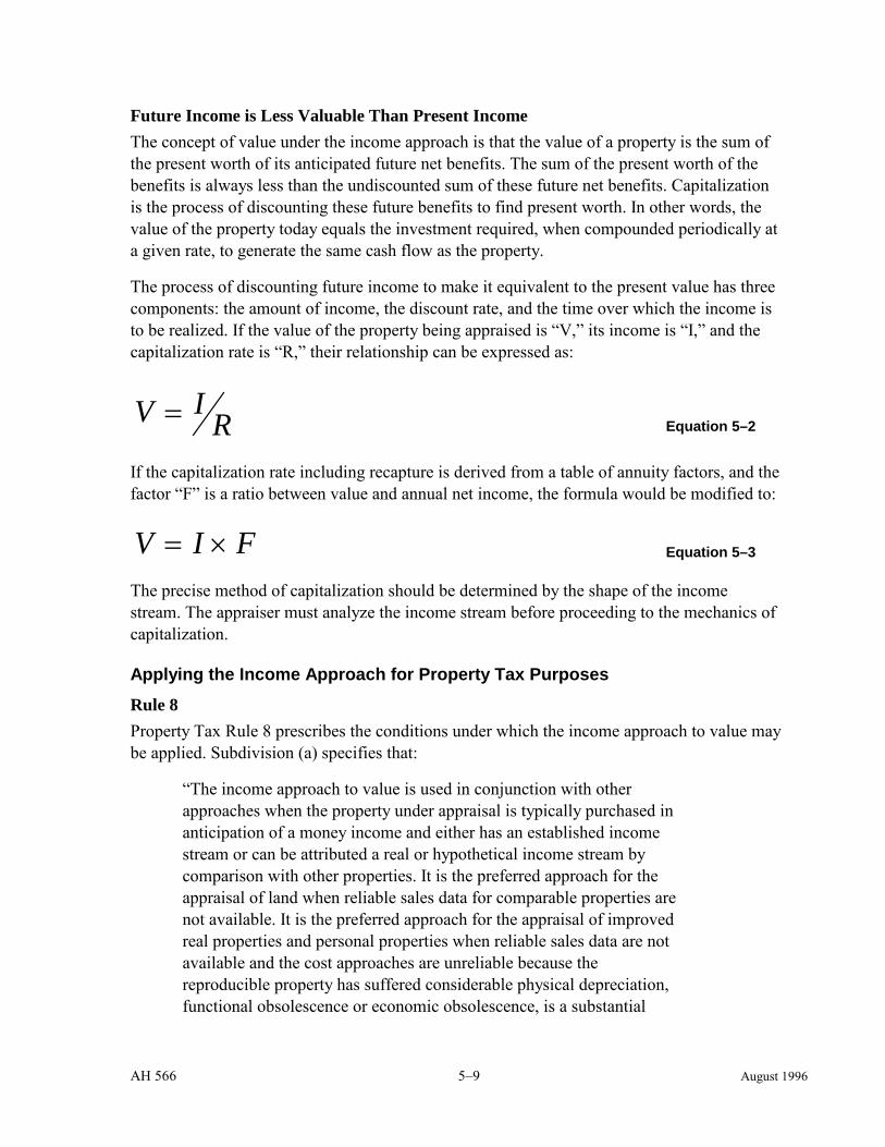
AH 566 5–9 August 1996

Future Income is Less Valuable Than Present Income The concept of value under the income approach is that the value of a property is the sum of the present worth of its anticipated future net benefits. The sum of the present worth of the benefits is always less than the undiscounted sum of these future net benefits. Capitalization is the process of discounting these future benefits to find present worth. In other words, the value of the property today equals the investment required, when compounded periodically at a given rate, to generate the same cash flow as the property.

The process of discounting future income to make it equivalent to the present value has three components: the amount of income, the discount rate, and the time over which the income is to be realized. If the value of the property being appraised is “V,” its income is “I,” and the capitalization rate is “R,” their relationship can be expressed as:

V IR= Equation 5–2

If the capitalization rate including recapture is derived from a table of annuity factors, and the factor “F” is a ratio between value and annual net income, the formula would be modified to:

V I F= × Equation 5–3

The precise method of capitalization should be determined by the shape of the income stream. The appraiser must analyze the income stream before proceeding to the mechanics of capitalization.

Applying the Income Approach for Property Tax Purposes

Rule 8 Property Tax Rule 8 prescribes the conditions under which the income approach to value may be applied. Subdivision (a) specifies that:

“The income approach to value is used in conjunction with other approaches when the property under appraisal is typically purchased in anticipation of a money income and either has an established income stream or can be attributed a real or hypothetical income stream by comparison with other properties. It is the preferred approach for the appraisal of land when reliable sales data for comparable properties are not available. It is the preferred approach for the appraisal of improved real properties and personal properties when reliable sales data are not available and the cost approaches are unreliable because the reproducible property has suffered considerable physical depreciation, functional obsolescence or economic obsolescence, is a substantial

AH 566 5–10 August 1996

over or underimprovement, is misplaced, or is subject to legal restrictions on income that are unrelated to cost.”

Subdivision (b) states that in using the income approach, “an appraiser values an income property by computing the present worth of a future income stream.” A complete description and practical application of such computation is set forth in the text.

Subdivision (c) establishes that the amount to be capitalized is the net return which a reasonably well informed owner and reasonably well informed buyers may anticipate on the valuation date that the taxable property existing on that date will yield, considering prudent management and subject to any legally enforceable restrictions as such persons may foresee as of that date. As stated therein:

“…Net return, in this context, is the difference between gross return and gross outgo. Gross return means any money or money’s worth which the property will yield over and above vacancy and collection losses, including ordinary income, return of capital, and the total proceeds from sales of all or part of the property. Gross outgo means any outlay of money or money’s worth, including current expenses and capital expenditures (or annual allowances therefor) required to develop and maintain the estimated income. Gross outgo does not include amortization, depreciation, or depletion charges, debt retirement, interest on funds invested in the property, or rents and royalties payable by the assessee for use of the property. Property taxes, corporation net income taxes, and corporation franchise taxes measured by net income are also excluded from gross outgo.”

Based upon the foregoing, while severance and other production taxes and/or permit fees are deductible, property taxes and income taxes are not legitimate deductions from gross income, nor are rents and royalties payable by the assessee for the use of the property.

Subdivision (d) states that in “valuing property encumbered by a lease, the net income to be capitalized is the amount the property would yield were it not so encumbered, whether this amount exceeds or falls short of the contract rent and whether the lessor or the lessee has agreed to pay the property tax.” Thus, the estimate of economic rent for income-producing property must be made without regard to actual lease arrangements that may exist, including rent levels and property tax considerations, since the objective is market value of the “unencumbered and unrestricted fee simple interest.”

Subdivision (e) recommends using income from property rental rather than business operation, since income derived from operation is more likely to be influenced by managerial skills and may arise in part from nontaxable property or other sources. If operating income must be considered, sufficient income must be excluded to provide a return on working capital and other nontaxable operating assets and to compensate unpaid or underpaid management.

AH 566 5–11 August 1996

Subdivision (f) requires the inclusion of a property tax component, equal to the estimated future tax rate for the area times the assessment ratio, in the capitalization rate for all property tax appraisals.

Subdivision (g) provides two means of developing a capitalization rate for property tax appraisals: (1) by comparing the net incomes that could reasonably have been anticipated from recently sold comparable properties with their sales prices, adjusted, if necessary, to cash equivalents (the market-derived rate); or (2) by deriving a weighted average of the capitalization rates for debt and for equity capital appropriate to the California money markets (the band-of-investment method) and adding increments for expenses that are excluded from outgo because they are based on the value that is being sought or the income that is being capitalized. In the former, the appraiser determines the ratio of net income to adjusted selling prices of comparable sales to develop a range of yield or overall rates, and subdivision (g)(1) states that this method is preferred when the required sales prices and incomes are available. In the latter, the appraiser derives a weighted average of current rates for debt and equity capital (subject to the inclusion of a property tax component).

Finally, subdivision (h), as previously discussed, provides that income may be capitalized by the use of gross income, gross rent, or gross production multipliers (derived by comparing sales prices of closely comparable properties with their gross income, gross rent, or gross production), and subdivision (i) excludes LCA (Land Conservation Act) properties and taxable possessory interests from certain provisions of Rule 8.

Discounted Cash Flow Analysis

Definition Discounted cash flow (DCF) analysis is a widely used “modern” form of capitalization that derives its validity from one of the most “old fashioned” principles of appraisal: the concept of present value. This concept asserts that present income is more desirable than future income, and that because investors prefer immediate cash returns over future flows, they discount future payments to their present worth.

DCF analysis is defined as the analysis of cash flow projections for each period of time that the property produces income in order to compute the present value of property assuming a certain rate of return or to compute the internal rate of return indicated by serial cash flows.

Although Rule 8 does not specifically mention DCF analysis, it is indirectly described and sanctioned in subdivision (b) by reference to an ideal income stream that is divided into annual segments, present worthed, and algebraically summed to determine the present worth of the total income stream.

Methodology To apply DCF analysis to an income-producing property, the appraiser must specify the quantity, variability, timing, and duration of the income stream as well as the amount and timing of the final cash flow (reversion), then discount each future payment to its present

AH 566 5–12 August 1996

value at a specified yield rate. In practice, most DCF analysis is done with financial tables (reversion and annuity factors) or with computer programs that incorporate these tables.

Since each year’s net income is viewed separately, the appraiser can tailor the projections of cash flow to recognize nonrecurring expenses, such as replacement of short-lived building components or clean-up of contaminated land in specific future years. This freedom from the constraints inherent in other forms of capitalization (e.g., level annuity) makes DCF analysis appropriate for irregular as well as regular patterns of income.

The mechanics of the discounting process in DCF analysis is a small part of the total process, especially with computer assistance. The appraiser must prepare detailed spreadsheets showing itemized cash flow projections, year by year or month by month, over the estimated life of the property. These flows are then discounted at some required rate of return to obtain total present value. The point is to account for the entire cash flow, in and out of the property, according to the timing of receipts and payments, so that the time value of money is properly recognized. When a desired rate of return is established, an investor can project the cash flows from a property, discount them to net present value, and therefore, determine how much to pay for the property in order to achieve the desired return.

Although DCF analysis is used frequently to solve for present value, given a rate of return, it can also be used to solve for an internal rate of return, given a purchase price, the amount of development capital, and the cash flow forecasts. When it is used for this purpose, DCF analysis is called IRR (internal rate of return) analysis.

For a more detailed explanation of the discounted cash flow process and related theory, see Appendix C.

AH 566 6–1 August 1996

Chapter 6 : PROPERTY TAX VALUATION

PROPOSITION 13

Proposition 13 (Article XIIIA California Constitution, Section 1) establishes that the maximum amount of any ad valorem tax shall not exceed one percent (1%) of the full cash value of the property. Under Article XIII A, Section 2, the full cash value means “the county assessor’s valuation of real property as shown on the 1975-76 tax bill under ‘full cash value’ or, thereafter, the appraised value of real property when newly constructed, or a change in ownership has occurred after the 1975 assessment.” As previously stated, the base year value can be adjusted for the effects of inflation up to a maximum of 2 percent per year based on the California Consumer Price Index. Table 6–1 lists the allowable inflation adjustment for each year since Proposition 13 was passed.

Table 6–1 Allowable Percentage Inflation Adjustment Based on the California Consumer Price Index

Year Allowable Adjustment 1979 2 1980 2 1981 2 1982 2 1983 1 1984 2 1985 2 1986 2 1987 2 1988 2 1989 2 1990 2 1991 2 1992 2 1993 2 1994 2 1995 1.19 1996 1.11

In judicial proceedings concerning the meaning and validity of Proposition 13 as it applies to the assessment of petroleum properties, the Court of Appeal held that although the acquisition value method of taxation is problematical, Rule 468 as adopted by the Board is an appropriate interpretation of Proposition 13 to oil and gas interests, since they have no real parallel to other types of real property. See Lynch v. State Board of Equalization, 64 Cal.App. 3d 94, 96 (1985), summarized in Appendix B.

AH 566 6–2 August 1996

REVENUE AND TAXATION CODE SECTION 51

Enacted for purposes of implementing Article XIII A, Section 2 (b) and Section 110.1, the provisions of Section 51 require that the lower of market value or the adjusted base year value be placed on the tax roll. This has an impact on petroleum property assessments, as they are reevaluated each year in order to reflect changes in development, economics, and technology.

PROPERTY TAX RULES APPLICABLE TO PETROLEUM PROPERTIES

RULE 2 Property Tax Rule 2, as discussed in Chapter 5, amplifies the definitive value concept in Section 110 and 110.1, that property is to be valued as if it were an unencumbered or unrestricted fee simple interest (subject to any legally enforceable government restrictions) “that would transfer for cash or its equivalent under prevailing market conditions between parties who have knowledge of the uses to which the property may be put, both seeking to maximize their gains and neither being in a position to take advantage of the exigencies of the other.”

RULE 4 Property Tax Rule 4 discusses the comparative sales approach to value whereby reliable market data in the form of sales prices from comparable properties are available. When such market data exists, this is the preferred method of valuing a property for ad valorem taxes. A recent sale of the subject property is the best indicator of value an appraiser will find. However, due to the low number of sales and the numerous variables for petroleum properties, very few petroleum property appraisals are made using the comparable sales approach.

RULE 8 Rule 8 discusses the income approach to value, which is the method used most often by petroleum property appraisers. The guidelines established in Rule 8 include examples of what is and is not to be included in the income stream and how the discount rate used should be derived. Lynch v. State Bd. of Equalization, p.109, recognized the application of Rule 8 in the valuation of oil and gas properties in stating,

“Rule 468 … retains a capitalization of income system of valuation based upon proved reserves. However, it modifies the prior practice in important aspects. Essentially the rule treats additions to proved reserves due to changed physical or economic conditions as additions to the real property interest. These reserves are valued as of the time they first become proved reserves, and are thereafter ‘frozen’ in value, subject only to the two percent inflationary increase permitted by

AH 566 6–3 August 1996

Article XIII A. In practice, at each annual reassessment the value of the oil and gas interest is reduced by depletions from the prior year’s production, adjusted for the 2 percent inflationary increase, and increased by the current value of new proved reserves. The additions to the proved reserves are thereafter ‘frozen’ in value pursuant to Article XIII A.”

RULE 21, POSSESSORY INTEREST DEFINITIONS Under Rule 21 a grant of a leasehold estate, an easement, a profit a prendre, or any other equitable interest of less than freehold, regardless of how it is identified in the document by which it was created, confers a right of possession that is independent, durable, and exclusive of rights held by others (as defined in Section 107) in nontaxable publicly owned property is a taxable possessory interest. The creation, assignment, or sublease of possessory interests are changes in ownership regardless of their term (Section 61(b)).

Such leasehold estates may be for a fixed term with an option of renewal, but they typically provide for a fixed term with a provision for continuance as long as the lessee is able to produce oil or gas in “paying quantities.” Since “paying quantities” generally means a profit, when the lessee can no longer produce hydrocarbons at a profit, the lease terminates and the rights revert to the public landowner. California courts have consistently held that the mineral rights of the lessee should be separately assessed to the lessee, since the lessee is the only “owner” of taxable real property and the lessor’s interest is tax exempt. Under Section 107, when the rights of the lessee are in nontaxable publicly owned land, they are to be placed on the secured rather than the unsecured roll.

RULE 22, CONTINUITY OF POSSESSORY INTERESTS Rule 22 provides that the continuity of, or exclusive use necessary to establish that a possessory interest exists, is satisfied when the possessor of the property uses it to substantially the same extent as would an owner engaged in the same activity. Standards for determining a possessory interest based on continuity are set forth in the rule.

RULE 23, WRITTEN AGREEMENTS AS TO THE TERM OF POSSESSORY INTERESTS Whenever a written agreement creating a possessory interest specifies a period of occupancy, the stated period shall be considered as the term of possession for valuation purposes under Rule 23. An option period shall be considered part of the stated term, if one may reasonably conclude it will be exercised. Subdivision (b) provides the assessor the latitude of presuming a term of possession that is reasonable subject to certain guidelines, when there is a conflict concerning the reasonably anticipated term or when there is no term stated.

RULE 24, POSSESSORY INTEREST RIGHTS TO BE VALUED Rule 24 states that the taxable value of a possessory interest is the sum of the value of all property rights in land and improvements held by the possessor, and that this value “is not

AH 566 6–4 August 1996

diminished by any obligation to pay rent or to retire debt secured by the possessory interest.” The rule also identifies examples of rights held by the public owner.

RULE 27, VALUATION OF POSSESSORY INTERESTS FOR THE PRODUCTION OF HYDROCARBONS. The taxable value of possessory interests for the production of gas, petroleum, and other hydrocarbons shall be determined by the application of the comparative sales or income approach as described in Rule 25 (a) or (b), except if the interest was created or last extended or renewed on or before July 26, 1963, and has been extended or renewed thereafter under authority which prohibits reduction of the rate of royalty to share in production because of an increase in the assessed value of such interests. Subdivision (a) sets forth valuation of such possessory interest under the comparative sales approach and subdivision (b) sets forth the income approach.

RULE 28, EXAMPLES OF TAXABLE POSSESSORY INTERESTS One of the commonly encountered taxable possessory interests is the “right to explore for, capture, and reduce to possession gas, petroleum, and other hydrocarbons in public lands.”

RULE 121, LAND The term “land” is defined in relevant part as “the possession of, claim to, ownership of, or right to possession of land; mines, quarries, and extracted mineral products…”

RULE 122.5, FIXTURES A fixture is defined as an item of tangible property, the nature of which was originally personalty, but which is classified as realty for property tax purposes because it is physically or constructively annexed to realty with the intent that it remain annexed indefinitely. Intent is the primary test of classification. Intent is measured with — not separately from — the method of attachment or annexation. Intent must be inferred from what is reasonably manifested by outward appearance.

RULE 124, EXAMPLES [OF LAND] The classification of items of property which constitute “land,” as distinguished from “improvements,” is set forth in the rule. Oil and water wells are listed under “LAND” in subdivision (a). Compressors, fences, and buildings are listed under “IMPROVEMENTS’ in subdivision (b).

RULE 468 Property Tax Rule 468, subdivision (a) specifically provides that the right to remove minerals from the earth is a taxable real property interest. Changes in the recoverable amounts of minerals will change the value of that interest. Proved reserves are defined and the steps to ensure that property values are estimated in accordance with Article XIII and Article XIII A

AH 566 6–5 August 1996

of the California Constitution are detailed. (Lynch V. State Board of Equalization, Appendix B.)

Pursuant to Rule 468, the base year value for proved reserves must be adjusted annually to account for production and other changes to proved reserve numbers, and new construction and equipment removal must be accounted for.

The valuation procedures set forth in Rule 468 are as follows. First, the total current market value of the property is estimated. Values for the wells, improvements, and surface equipment actively used in property operations are determined and subtracted from the total value (becoming an offset). The result is the current taxable value of the reserves.

The volume of any change in proved reserves is estimated by subtracting the prior year’s reserves, less last year’s production (depletion), from the current estimate of reserves for the property.

The value of produced reserves is determined by multiplying the volume of the prior year’s production by the weighted average value of reserves for all prior base years. The taxable value of the prior year’s reserves remaining is found by subtracting the value of the prior year’s production from the prior year’s taxable value of reserves. The value of the change in reserves from other than production is found by multiplying the change in volume by the current market value per unit of the total reserves.

The current base year value for the reserves is the sum of the value of the prior year’s reserves, less depletion, appropriately factored for inflation, added to the value of the changed reserves.

The base year value for land (other than mineral rights) and improvements is the value on lien date 1975, the date of new construction or the date of a change in ownership subsequent to 1975. The base year value is factored each year the same as other real property in the state; however, if in any year the value declines below the adjusted base year for the total property, then the lower value is placed on the roll for that year.

SECTIONS 75 – 75.40 – SUPPLEMENTAL ASSESSMENT

Commencing on or after July 1, 1983, whenever a change in ownership occurs or any new construction resulting from actual physical new construction on the site is completed, the assessor is required under Sections 75 – 75.40 to appraise the property changing ownership or the new construction at its full cash value (except as provided in Section 68(b)) on the date the change in ownership occurs or new construction is completed. Section 75.11 prescribes the dates and the differences in value to be placed on the supplemental tax roll. Only the difference in value beyond the lien date roll value is measured. When evaluating an event for supplemental assessment, two questions need to be addressed. First, has new construction or a change in ownership taken place? Second, what is the change in value attributable to the

AH 566 6–6 August 1996

assessable event? If the answer to the first question is negative, then there is no need to ask the second. In the case of new construction, only the value attributable to the new construction is to be enrolled as a supplemental assessment.

While drilling new wells, installing flow lines, and constructing surface production facilities will normally constitute “new construction” as that term is used by SBE Rules 463 and 463.5, such activity may not increase the value of the property for the purposes of levying a supplemental assessment. In other words, a supplemental assessment occasioned by such construction may be zero.

NEW DISCOVERIES Section 75.10(c) specifically states that new discoveries of previously unknown reserves of oil and gas are to be treated as “actual physical new construction” for the purposes of the supplemental roll. Reserves, however, are not to be treated as construction in progress. Once the reserves (or additions to reserves) have been discovered and “proved” per Rule 468(b), they must be quantified and appraised, and a base year established.

NEW CONSTRUCTION Property Tax Rules 463 and 463.5 govern how new construction is classified and enrolled. New construction associated with petroleum properties includes the drilling or deepening of wells, recompletions in new zones, the installation of flow lines, and construction of surface production facilities.

Additions Additions to the proved reserves and newly constructed improvements shall be valued as of the lien date of the year for which the roll is being prepared. The new reserves are valued by multiplying the new volume (determined by subtracting the prior year’s reserves, less depletions, from the estimated current total reserves) by the current market value per unit of the total reserves. (Rule 468(c)(4)(E).) The added reserves, once “proved,” are new property that did not exist before, and thus cannot be treated as construction in progress.

Replacements The substitution of an item which has become exhausted, worn out, or inadequate with one of fundamentally the same type or utility is a replacement. For property tax purposes, construction or reconstruction of an improvement or fixture performed for the purpose of normal maintenance and repair, (e.g. routine annual preparation of agricultural land, interior or exterior painting, roof covering replacement, the addition of aluminum siding to improvements, or the replacement of worn machine parts) constitutes replacement rather than “new construction.” (Rule 463(b)(4).) The effects of maintenance and repair may be reflected in the market value estimate of the property, but the property retains its original base year value without any addition for the costs of the maintenance and repair.

AH 566 6–7 August 1996

Replacements can be so extensive and extreme, however, as to make an improvement “like new.” Section 70(b) of the Revenue and Taxation Code provides that “new construction” includes: “Any rehabilitation, renovation, or modernization which converts an improvement or fixture to the substantial equivalent of a new improvement or fixture is a major rehabilitation of such improvement or fixture.” (Emphasis added.) Also see Rule 463. If the fixture or improvement is reconstructed to the substantial equivalent of new, the item is to be appraised at fair market value as of the date of completion (see Rule 463(b)). The original base year value of the item is removed and a new base year value is enrolled. The difference in value between the newly reconstructed item and the current value on the roll is enrolled as a supplemental assessment.

Timely replacement of property damaged by misfortune or calamity does not fall under the definition of assessable new construction (Section 70(c) and Rule 463(f)). However, if the replacement property is not substantially equivalent to the property before the damage, a portion of the replacement will be taxable. See Rule 463(f).

Property tax relief for damage from a misfortune or calamity is only available if the county, where the property is located, has adopted a disaster relief ordinance. Since a timely replacement of a property damaged by misfortune or calamity is not new construction, it is not subject to supplemental assessment. Such a reconstructed improvement or fixture retains the base year and base year value of the original. However, if the property receives immediate relief in assessed value as a result of the calamity, the replacement is enrolled and taxed upon completion. Although technically there is no supplemental assessment in such a case, supplemental assessment procedures are used for enrolling and taxing the completed replacement. See Section 170, Revenue and Taxation Code.

Appraisal judgment, based on consideration of the relevant facts, must be exercised to determine whether the construction or rebuilding of an improvement or fixture is (1) taxable as new construction, (2) partially assessable as new construction, or (3) non reappraisable as restoration or replacement. It is obvious from the foregoing that it is not always clear whether construction or rebuilding of an improvement or fixture is new construction, is partially assessable as new construction, or is not new construction.

In the case of petroleum properties, “replacement wells” can be particularly difficult to classify as assessable new construction versus calamity replacement.

A “replacement well” can refer to replacement of a well that failed due to an unexpected, calamitous event, or to replacement of a well that has suffered a decline in production due to things such as reduction in pressure available or a change in the relative permeability of the formation. Furthermore, in a calamity case, the operator may choose to sink the replacement well in a new location that will tap both the original area of the well that failed plus an adjoining area where a future well was anticipated prior to the calamity.

When the original well fails due to pressure decline, loss of permeability, or any reason other than calamity, any replacement well is “new construction” and is subject to supplemental

AH 566 6–8 August 1996

assessment upon completion. The base year value of the original well is removed from the assessment when the well has been officially abandoned. For property tax purposes, the replacement well is treated as an entirely new property and is not related to the original well.

In the case of a calamity, a replacement well drilled to recover the same petroleum as the original well would have recovered is not “new construction.” The replacement will carry the base year value of the original well. “To recover the same petroleum” means that the replacement well bottom is in approximately the same location as the original. Note that in some cases it is not feasible to drill the well at the same surface location.

If a well fails due to calamity and the operator drills a replacement that will both tap the area of the failed well and some additional area, the assessment should be prorated as provided by Rule 463(f).

REMOVAL OF PROPERTY Supplemental assessments can result in negative changes in value. This would be the case if property were “removed.” A well that is capped—permanently abandoned—is considered to be removed, resulting in a negative supplemental assessment.

Section 75.10(b) provides in relevant part:

“For purposes of this chapter, “actual physical new construction” includes the removal of a structure from land.

Property Tax Rule 463 requires that the new full cash value shall be computed as of the date of completion for only the newly constructed portion, and that the taxable value shall be determined by adding the full value of the new construction to the taxable value of the preexisting property, less an amount for the taxable value of property removed during construction.

SECTION 607.5 – ASSESSABLE MINING RIGHTS OR MINERAL RIGHTS

Whenever a separate assessment of rights and privileges pertaining to mines or minerals and land is made, the words “mining rights” or “mineral rights” on the roll shall include the right to enter in or upon the land for the exploration, development, and production of minerals, including oil, gas, and other hydrocarbons. See Section 607.5.

AH 566 7–1 August 1996

Chapter 7 : APPRAISAL OF WELLS, INSTALLATIONS, AND EQUIPMENT

Petroleum properties require wells and equipment in order to remove the petroleum from the earth and move that petroleum from its source to the sale point. Although petroleum properties are valued as a unit, wells, other improvements and equipment must be listed, appraised, and assessed separately from the mineral rights.

The purpose of this chapter is to provide guidelines on the appraisal and assessment of wells and fixed equipment associated with the production, storage, and initial transportation (pipelines and associated fixed equipment) of unrefined petroleum.

WELLS

The term “well” includes the shaft sunk into the earth and the permanent, non-recoverable casing. Wells are assessed (classified) as land.1 Unlike most other types of land, however, wells are subject to appraisal depreciation to the extent that (1) their values are related to the value of the mineral rights and/or (2) they suffer physical damage, destruction, and/or economic obsolescence.

PRODUCTION EQUIPMENT

The term “production equipment” includes removable equipment used between the bottom of the well and the header, such as tubing, well heads, artificial lifts, flow lines, and the various components of these items. Production equipment items are classified as fixtures, since they are physically annexed to real property with the intent to remain so indefinitely.2 These items can be removed for repair and replacement. At the end of the life of the well, some of the items may have a value to the extent they can be removed and reused at another site. Other items may have no net value or may have a negative value (when required to be removed and the cost of removal exceeds the net salvage value).

SURFACE FACILITIES

The term “surface facilities” includes all that equipment from the header to the tanks, such as separators, dehydration systems, storage systems, and the various components of such items. Surface facilities also include structures, such as field offices, control rooms, etc. and equipment, such as filters, pumps, flow lines, and tanks.

1 Rule 124, California Code of Regulations, Title 18. 2 See Rule 122.5, California Code of Regulations, Title 18.

AH 566 7–2 August 1996

Surface facilities provide the chemical and physical means of separating the production fluids. Fluids produced from an oil well are a combination of oil, gas, water, and solids, and they must be separated and measured before the oil and gas can be sold. (Separation is also important for safe handling and storage prior to sale.)

The petroleum mixture will dictate the design of the production facilities. Fields that produce a high water content may require vessels called “free water knockouts.” For fields with oil and water emulsions, a heater treater may be required. Heater treaters use the application of heat and chemicals to break down the oil and water emulsion.

Surface facilities are physically annexed to real property and are classified as fixtures. Compared to production equipment, surface facilities may have a positive residual or salvage value at the end of the life of the well or field. However, some or all of the equipment may have no value or negative value depending on the costs of removal, transportation, and reinstallation at another site, as well as the suitability of the old equipment as compared to new equipment or other available alternatives.

APPRAISAL OF OIL FIELD PRODUCING EQUIPMENT

The appraisal of oil field producing equipment and non-producing equipment is initiated by the operator reporting the equipment, and verified by the appraiser making a detailed field check. A field check is preferable when the lease is first put into production, enabling the appraiser to determine whether specialized valuations are needed. In subsequent years, the operator reports changes that have occurred to the equipment, and supplemental field checks by the appraiser are conducted as conditions warrant. All equipment in use on the lease should be itemized. If known, it is important to record the age of the equipment, as it may be of use in determining value.

Common practice for the appraisal of the well and production equipment is to tie the value directly to its estimated utility to extract petroleum. A remaining reserve factor is determined by taking the estimate of proved reserves and dividing by the total ultimate recovery. Then multiply this factor by the cost of a new well with the current equipment. As reserves are produced, the value of the equipment will decline in direct proportion.

The most practical way to appraise the surface facilities is to use the original cost and original year of acquisition as a starting point. The original cost is multiplied by an index factor found in Assessors’ Handbook Section 581. The result is reproduction cost new (RCN). A percent good factor is then applied to the RCN to arrive at an estimate of fair market value.

Within certain limits, the equipment being used on a well should last as long as the well is capable of producing. The estimated life of a well may be 20 years or longer. Normally, equipment used on the well is given an average life of 20 years. When determining the remaining economic life of a piece of equipment, the appraiser’s judgment should be used.

AH 566 7–3 August 1996

A guide in making an appraisal on machinery and equipment is that replacement cost new–including the full current costs of engineering, the equipment, applicable sales taxes, freight-in, overhead, interest during construction, and installation–is generally considered as the upper limit of value. In some cases, the use of indexing will result in a reproduction cost estimate that, even after allowing for depreciation (the percent good calculation), exceeds current replacement cost new. When this occurs, or in situations where original costs and years of acquisition are unknown, it is necessary to use other methods to derive a reasonable estimate of value.

The equipment should be described in sufficient detail for accurate identification—manufacturer, model, size, length, or other description—before the valuation process can proceed. Oil field supply companies are excellent sources of information on recent cost data. Supply companies sell most of the equipment required to produce oil. Because each supply company has franchises from particular manufacturers, it may be necessary to contact several. If the supply companies do not stock a particular item, the distributors or operators may be contacted for cost data.

A reasonable rate of depreciation must be applied to the original cost to allow for physical wear and obsolescence. When the original cost or present value is difficult to establish because of the age of the equipment, appraisal information can usually be found by contacting another assessor in an oil producing county. The value of older equipment can also be determined by observing sales and/or by making a survey of the second hand market.

Prior to Proposition 13, accuracy in determining equipment values was not necessary because the total property value was not affected, only the allocation. Today, accurate determinations of value are more critical, because the value allocated to the mineral rights can have a long lasting effect on the base year for those reserves.

Variations can be made on the depreciated cost of equipment (or fair market value based on a market survey) as a means of making an appraisal. Some examples are: tanks at a per barrel rate; engines at a value per cubic inch of displacement; pumping units at a value per 1000 pounds of beam capacity; pumps at a value for each inch of the diameter of the discharge port; or gas traps at a value per cubic foot. Full reliance on appraisals based on such ratios is not advised, since the equipment is valued for its utility without consideration for its age or condition, and therefore lacks accuracy. However, an appraisal of this type may be practical when used in conjunction with a total property appraisal.

FUNCTIONAL OBSOLESCENCE Decreases in productivity as a field ages can result in functional obsolescence on portions of the equipment that were in full use when the facility was first put on-line. Failure to recognize the functional obsolescence of the surface facilities can lead to an improper allocation of the value and result in improper assessments. Functional obsolescence could be subcategorized as superadequacy.

AH 566 7–4 August 1996

It is tempting but incorrect to think of superadequacy as any capacity in excess of that which will be needed in the foreseeable future. Since petroleum properties are expected to decline in production over their economic lives, some excess capacity is normal as the properties age. In the case of production equipment, the effect of normal excess capacity is captured because the equipment value is tied to the remaining reserves, as described above. In the case of surface facilities equipment, the percent good tables published in Assessors’ Handbook Section 581 include an allowance for normal functional obsolescence.

Although there is no precise definition for superadequacy for surface production facilities, an allowance for superadequacy should be considered when the current and projected use of the equipment is significantly below design capacity. Superadequacy only exists if the excess capacity will not be used in the future. If there are further development plans for the property that will increase production, the amount of the superadequacy is only the amount of the excess capacity above the expected peak production levels. Appraisal judgment must be exercised.

Determining the value of the superadequacy for a field installation is sometimes impractical. It would require reengineering the facilities layout, determining the proper size of the equipment and whether satisfactory substitutions could be made, and analyzing the economic feasibility of correcting the superadequacy.

Instead, the following procedure is recommended, assuming information is available on the cost to correct the superadequacy and the correction is economically feasible. (1) Determine the reproduction cost of the current installation. (2) Calculate the depreciation charge. (3) Determine the cost to remove the excess capacity and install the properly-sized equipment. (4) Subtract the depreciation charge and the cost to cure the superadequacy. The remaining value represents the loss in value from depreciation and functional obsolescence.

It should be pointed out that since petroleum properties are valued as a whole, the primary reason for making an adjustment for superadequacy or other forms of obsolescence is for purposes of allocation. Where superadequacy exists, subtracting the normal fair market value of the equipment may leave little or no value for the petroleum reserves. Since the reserves must have some value if the well is producing or is expected to produce, it is necessary to recognize equipment obsolescence so the total value can be allocated reasonably.

IDLE EQUIPMENT

The equipment discussed to this point has been regarded as making a direct contribution to production. An appraisal of the idle equipment on the property is also required, since many properties retain such equipment for numerous reasons.

The term “idle equipment” includes two distinct categories: (1) equipment that does not contribute directly to the anticipated cash flow of a property but may be needed if certain

AH 566 7–5 August 1996

conditions occur in the future; and (2) equipment that has no use on the property today or in the foreseeable future.

Since idle equipment does not contribute directly to the anticipated cash flow of a property, it is not included in the value determined by the cash flow analysis. The equipment has some value—replacement parts or scrap—however, in the event of a sale of the property.

The value of idle equipment that may be used in the foreseeable future is typically between salvage value and the value of similar equipment in use. In such cases, the value should be the normal value less some allowance for deferral and/or risk. Since the equipment has no current income-producing ability and only a possibility of a future role in production on the property, its value must be less than it would be if the equipment were part of the current cash flow. Professional appraisal judgment must be used in applying specific methods for appraising such equipment.

Idle equipment that will not be used for the property—known as “Idle Equipment Waiting on Abandonment”—is usually valued closer to salvage value. In the appraisal of such idle equipment, since it is presumed that it will never be used on the property, installation costs should not be included in the value. In addition, the appraiser needs to allow for items such as the condition of the equipment, repairs made and/or needed, age of the equipment, and the total life expectancy of the equipment.

When cost or life data is incomplete or not available, reference to schedules of assessed values and market values prepared by the assessors of other oil producing counties is advisable in making a determination of market value. Additionally, sales studies and a survey of the second hand market would be appropriate.

APPRAISAL EXAMPLE

The following is an example of an appraisal of equipment on a small oil field production facility. The appraisal is for the March 1, 1995 lien date, on a facility consisting of three wells, pumping units for two of the wells, a separator, a dehydrator system, a free water knockout, and four storage tanks. The free water knockout and one of the tanks were added in 1992 to handle increased water production. Only two tanks are needed for the current level of production of the field, but as more water is produced the third tank will be needed.

The fourth tank is not expected to be needed and is idle waiting on abandonment. The cost to remove it is estimated at $1,250. The cost to drill and complete a flowing well is $120,000. Pumping units are $32,000 per unit. Remaining reserves are 72 percent of the ultimate recovery. The property was put into production in 1987. The list below details the cost of the surface facility.

AH 566 7–6 August 1996

Description Year Acq Cost

Separator 1987 15,000

Free Water Knockout 1992 12,000

Dehydrator 1987 1,000

Tank 1987 7,000

Tank 1987 7,000

Tank 1992 7,700

Tank 1992 7,700

Miscellaneous Pipes and Fittings 1987 2,000

Miscellaneous Pipes and Fittings 1992 500

The numbers are not representative of what the actual items cost but are used only for the purposes of this illustration. Likewise, the equipment listed should not be interpreted as the required installation but as an example of the types of equipment that could be found on a property.

For this appraisal, the appraiser used the Industrial Group 3 index from the 1995 edition of Assessors’ Handbook Section 581. The percent good figures are based on a 20-year life and came from Table 5 therein.

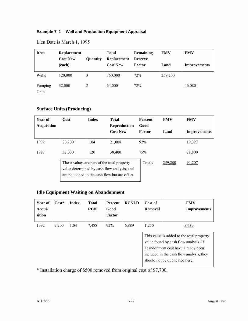
AH 566 7–7 August 1996

Example 7–1 Well and Production Equipment Appraisal

Lien Date is March 1, 1995

Item Replacement Cost New (each)

Quantity

Total Replacement Cost New

Remaining Reserve Factor

FMV Land

FMV Improvements

Wells 120,000 3 360,000 72% 259,200

Pumping Units

32,000 2 64,000 72% 46,080

Surface Units (Producing)

Year of Acquisition

Cost Index Total Reproduction Cost New

Percent Good Factor

FMV Land

FMV Improvements

1992 20,200 1.04 21,008 92% 19,327

1987 32,000 1.20 38,400 75% 28,800

These values are part of the total property value determined by cash flow analysis, and are not added to the cash flow but are offset.

Totals 259,200 94,207

Idle Equipment Waiting on Abandonment

Year of Acqui-sition

Cost*

Index Total RCN

Percent Good Factor

RCNLD Cost of Removal

FMV Improvements

1992 7,200 1.04 7,488 92% 6,889 1,250 5,639

This value is added to the total property value found by cash flow analysis. If abandonment cost have already been included in the cash flow analysis, they should not be duplicated here.

* Installation charge of $500 removed from original cost of $7,700.

AH 566 8–1 August 1996

Chapter 8 : PETROLEUM PROPERTY APPRAISAL METHODS

The reserves estimate and the forecast of how those reserves will be produced is the most important part of any petroleum property appraisal. Once a forecast of production is available, the appraiser can develop a cash flow model of the property. For most petroleum properties, the income approach to value should be used, and employing an appropriately supported discounted cash flow analysis will produce a good approximation of fair market value.

FORECASTING OIL PRODUCTION

As discussed in Chapter 2, for properties that have sufficient production to establish a decline trend, production can be forecast by extrapolating the trend. For those properties where a decline has not been established, another forecasting method must be used. Consultations with a petroleum engineer or petroleum geologist or a forecast obtained from the property operator may be a practical necessity.

For those properties where a decline in production is well established, the appraiser can use the formulas shown in Chapter 3 to extrapolate future production. Most of the petroleum properties in California will fall into this category.

FORECASTING GAS PRODUCTION – SPECIAL ISSUES

When dealing with gas properties, some special considerations are necessary for accurate appraisals.

AN UNCONNECTED GAS WELL Frequently, when a new gas well is drilled, the discovery is insufficient by itself to justify the expenses of a gas sales pipeline. The well is shut-in, closed at the well head, pending further field development. The question often raised is what is the assessable value of the well? What value should be enrolled?

Since there is no mechanism to bring the gas to market, proved reserves do not yet exist for the well. The value of the improvements, the well, and any site improvements, are assessable at their value. However, no assessment for proved reserves can be made until there is a reasonable expectation to connect the well to a pipeline. Once an expectation exists, the value of reserves should take into account the delay in connecting the well to the pipeline. The reserves should be classified as proved developed nonproducing.

AH 566 8–2 August 1996

CASH FLOW ANALYSIS

The following section covers most of the required information for a discounted cash flow analysis and the methods used to arrive at a value conclusion.

COMPONENTS OF A CASH FLOW

Developing a cash flow model for a property analysis is easier when it is broken into component parts. For any income stream there will be revenues, expenses, and a value determination.

REVENUES For traditional petroleum properties, there are typically three revenue streams to be addressed in the cash flow. These are oil sales, gas sales, and natural gas liquid sales. Additional revenue streams may exist, e.g., electricity and steam sales. Once the production forecast has been established, it is simply a matter of multiplying the forecast by the product price forecast and summing the revenue streams to arrive at total revenue.

Product Prices Oil is generally priced based on gravity and location.1 The refinery posting takes into account the various components of the crude oil and how processing this oil will affect the plant output. Attempting to forecast prices into the future is a formidable task. Considerable effort by the petroleum industry is put into developing price forecasts.

The price of all commodities like petroleum is related to supply and demand. Typically, if supply goes up and demand remains the same, prices drop until they reach an equilibrium level. The same occurs as supply goes down. Prices will increase until the demand levels off.

The oil price shocks of the seventies and eighties confirmed the commodity price structure of petroleum. As prices increased, consumers began to conserve. This, coupled with the increased exploration by producers, brought a glut to the market. In order to sell their production, companies and countries began accepting lower prices, rather than holding the production in inventory.

As long as a sufficient surplus in production exists, producers will not have any control over the price they receive. This situation is not unique to the recent past. The cycle of boom and bust has been reoccurring since the early days of the industry in Pennsylvania.

Revenue Summary Revenues are calculated by multiplying the net production times the product price for each year. On some properties, operators will use part of the production stream as fuel for the

1 Posted prices were discussed in Chapter 2.

AH 566 8–3 August 1996

operations. It is customary to deduct the oil or gas used for the operations from the production values, prior to determining revenues. Production rates for components of the production stream may be scheduled or may be based on ratios. The gas/oil ratio is the rate of gas production related to the rate of oil produced from a property. The NGL/gas ratio is the amount of natural gas liquids extracted per MCF of gas production. The property operator can supply these ratios, or they can be determined from the annual production statement.

Once the revenue components are calculated they can be summed to provide an estimate of total annual revenue for the property. Page 4 of Example 8–2 at the end of this chapter shows the revenue page of an appraisal spreadsheet.

EXPENSES All expenses that are related to and necessary for the operation of the property should be included in the cash flow analysis. There are five general classifications of expenses that concern the petroleum property appraiser. They are capital expenses, operating expenses, periodically reoccurring expenses, overhead expenses, and other non-reoccurring expenses. Expense data is reported by the operators in their annual property statements filed with county assessors. Expenses associated with other revenue sources should be included.

Capital expenditures are investments in equipment and improvements that will generate income for more than one period. Examples of capital expenses are tubing, wellheads, tanks, flow lines, separators, buildings and recompletion costs.

Expenses that will only benefit one period, the one in which they are paid, are called operating expenses. Examples of operating expenses are direct labor for lease operations, maintenance expenses, water handling costs, and workover.

Periodic reoccurring costs are those costs that will occur at regular intervals but not on an annual basis. An example of these types of costs are those associated with cyclic steaming or routine maintenance of larger equipment.

While all costs associated with the property should be included, they do not have to occur on the property. Overhead charges are included for certain expenses allocated from the division or corporate headquarters. Overhead includes salaries for management, engineering, and accounting that are necessary for the operation of the property. For the property tax appraiser, overhead costs are among the most difficult expenses to identify. The appraiser needs to be certain that only those costs directly attributable to the property are included. Also, certain costs, while legitimately attributable to the property, cannot be considered for property tax valuations. These include property taxes, amortization, depreciation, depletion charges, and rents and royalties for use of the property. (See Rule 8(c) and AH501A.)

Other non-reoccurring expenses include abandonment costs and environmental cleanup costs and will be discussed further below.

AH 566 8–4 August 1996

Fixed and Variable Operating Expenses Operating costs can be classified as either variable or fixed.

Variable costs change with respect to the level of fluid output or the number of wells. Generally, variable costs change in relationship to the activity level on the property (AH501A). Examples of variable costs are fluid treatment costs and some labor costs. As oil production decreases, some costs will decline. However, if there is increasing water production associated with the property, as oil production decreases, water disposal costs will increase. An analysis of variable costs should be made to determine the controlling variable.

Fixed costs are those expenses that do not change over short periods of time regardless of the changes in production.Such costs are typically fixed only for a certain range of production. When the production rate changes substantially, the fixed cost structure will also change. Fixed costs include salaries, rents, insurance, and leased equipment payments. These are costs typically paid even if there is no production.

Some costs will exhibit characteristics of both fixed and variable costs. For example, electrical expenses for oil companies typically have a fixed component for capacity availability and a variable component for actual electrical usage.

When trying to determine whether an expense is fixed or variable, the following questions should be asked: What would happen to this expense if production changed by one barrel per day? What would happen if the number of wells were changed by one? What would happen to this expense if the property did not exist? If the expense would not change with a change in the number of wells or a change in production, then it is likely to be a fixed expense.

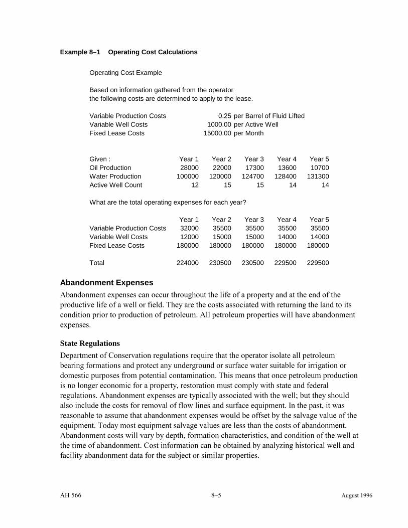
AH 566 8–5 August 1996

Example 8–1 Operating Cost Calculations

Operating Cost Example

Based on information gathered from the operator the following costs are determined to apply to the lease.

Variable Production Costs 0.25 per Barrel of Fluid LiftedVariable Well Costs 1000.00 per Active WellFixed Lease Costs 15000.00 per Month

Given : Year 1 Year 2 Year 3 Year 4 Year 5Oil Production 28000 22000 17300 13600 10700Water Production 100000 120000 124700 128400 131300Active Well Count 12 15 15 14 14

What are the total operating expenses for each year?

Year 1 Year 2 Year 3 Year 4 Year 5Variable Production Costs 32000 35500 35500 35500 35500Variable Well Costs 12000 15000 15000 14000 14000Fixed Lease Costs 180000 180000 180000 180000 180000

Total 224000 230500 230500 229500 229500

Abandonment Expenses Abandonment expenses can occur throughout the life of a property and at the end of the productive life of a well or field. They are the costs associated with returning the land to its condition prior to production of petroleum. All petroleum properties will have abandonment expenses.

State Regulations Department of Conservation regulations require that the operator isolate all petroleum bearing formations and protect any underground or surface water suitable for irrigation or domestic purposes from potential contamination. This means that once petroleum production is no longer economic for a property, restoration must comply with state and federal regulations. Abandonment expenses are typically associated with the well; but they should also include the costs for removal of flow lines and surface equipment. In the past, it was reasonable to assume that abandonment expenses would be offset by the salvage value of the equipment. Today most equipment salvage values are less than the costs of abandonment. Abandonment costs will vary by depth, formation characteristics, and condition of the well at the time of abandonment. Cost information can be obtained by analyzing historical well and facility abandonment data for the subject or similar properties.

AH 566 8–6 August 1996

Accounting For Abandonment Expenses It should not be assumed that funds will be available for abandonment costs from other sources. Abandonment costs are specific to each property and should be paid for out of each property’s cash flow. The allocation should be enough so that the full cost of abandonment is available when the property has reached its economic limit. The appraiser should not make the assumption that abandonment costs will occur after the economic limit has been reached.

Abandonment expenses may be accounted for by establishing a sinking fund account. The purpose of this account is to set aside funds each year. These funds grow to a predetermined amount by the time they are needed to pay for the cost of abandoning the property.

Environmental Expenses Related to abandonment expenses are other environmental clean up costs associated with a property. Only those environmental costs related to the mineral extraction operations of the property should be considered. These may include the costs to remove and replace contaminated soil, removal of leaking tanks, and monitoring of the environmental hazards. The effect of environmental cleanup costs resulting from other operations on or near the property should be accounted for in the surface value of the land. The typical requirement for environmental liability today is to restore the property to its original condition. Environmental costs should be treated the same as abandonment costs in the cash flow. The expenses should be estimated, adjusted for inflation, and a sinking fund allocation established. See also Firestone Tire & Rubber Co. v. County of Monterey, 223 Cal.App. 3d 382 (1990), Appendix B.

Benchmarking The practice of benchmarking has developed and increased for all types of industries over the last decade. The concept of benchmarking for business purposes is to identify an industry leader and compare its costs of operations to your own. When properly done it helps managers to identify areas of their operation that can be improved and highlight areas where no additional effort is needed.

In regard to petroleum property appraisals, benchmarking should be applied on a broader scale. Reasonable costs are calculated based on input from all operators in an area. Reasonable costs in a given area should include all classifications: operating, abandonment, and environmental. The comparisons should not be mixed and matched to develop the lowest or highest cost of operating a producing field. It is important to make certain that all allowable costs are included, since individual firms account for different expenses by differing methods. What one firm rolls into overhead may be categorized differently at another.

Royalty Deductions Property Tax Rules 4(b) and 8(d) state that all real property is to be appraised as though it were unencumbered by a lease, mortgage, or other private agreement. In Atlantic Oil Co. v.

AH 566 8–7 August 1996

County of Los Angeles, 69 Cal.App. 2d 585 (1968), the California Supreme Court held that the deduction of the present value of the right to future royalty payments was prohibited in the valuation of oil and gas leases under the income approach. Some government royalties are an allowable deduction from the cash flow when determining property values. Section 107.2 requires that the value of petroleum interests created prior to the decision in DeLuz Homes, Inc. v. County of San Diego (1955) 45 Cal.2d 546 shall exclude the value of any royalties or other rights to share production by tax exempt entities. Section 107.2 does not apply if the interest is extended or renewed unless the renewal was provided for in the lease and the lease does not allow a reduction in the royalty or production share due to an increase in the assessed valuation.

Expense Summary After all of the allowable expenses have been calculated, the annual net operating income can be determined. Assuming that the property is operated to provide income to the operator, the economic life of the property is the point where the net operating income becomes negative without any potential to return to positive. See Page 5 of Example 8–2.

VALUE DETERMINATION The final step in the cash flow analysis is the value determination. This is where the net operating income of the property is resolved into an expression of value.

Discount Rates In a cash flow analysis, the discount rate represents the required return investors need to accept a project. This is the combined rate that providers of capital, either debt or equity, require for putting their funds at risk, and the risk associated with the property.

The sum of the discounted cash flows typically represents the maximum value investors would pay for the projected income, given the risks associated with the income. At this maximum price the rate of return will equal the discount rate if the property performs and the cash flows occur as projected. When negotiating a purchase price, buyers will most likely seek a price below the present worth of their cash flow projections. The actual return experienced on the property may be greater than or less than the discount rate used to determine the purchase price. For information on the derivation of discount rates according to Rule 8, see Appendix C – Derivation and Estimation of Discount Rates Used in Discounted Cash Flow Analysis.

Discounting for petroleum properties is generally done using midyear factoring. The assumption is that the annual income will be received at the middle of the year. The formula

AH 566 8–8 August 1996

for midyear discounting is the same formula for end of year discounting with one small adjustment.2

Discount Factor =+ −

11 0 5( ) .i n Equation 8–1

where i = discount rate n = the number of years until payment received

Rule 8 requires that a before-tax discount rate be used. Taxes are excluded as a deductible item from the income stream because they are based on the income that is being capitalized. A component for property taxes must be added to the rate since these are also excluded as a deduction from the income stream.

Risk The concept of risk involves the following:

Table 8–1 Definitions relating to risk.

Term Definition

Outcome One of the possible events that can take place.

Probability The chance between 0% and 100% that a particular outcome will occur.

Certainty Only one possible outcome. 100% probability of occurrence.

Uncertainty Recognition that more than a single outcome is possible, with each outcome having a finite probability of occurrence.

Risk Possibility of incurring economic loss or reduced economic value.

Adapted from “Economics of Worldwide Petroleum Production” by Allen & Seba

The first three terms are commonplace, and the probability of those actions can easily be determined or estimated as with weather. By analyzing weather patterns and through satellite 2 There are several formulas for discounting income in a cash flow. Most spreadsheet programs use end of period discounting. Other methods are beginning of period and continuous. The type of discounting used is dictated by the practice of the industry and the actual timing of the cash flow.

AH 566 8–9 August 1996

imaging, meteorologists forecast outcomes in temperature, precipitation, and wind direction. The probability of the forecast actually occurring is based on the reliability of the input data and past history.

Uncertainty is not knowing the outcome of an event even though one may know the odds of a specific event occurring. Uncertainty can be further divided into objective uncertainty and subjective uncertainty. Objective uncertainty can be calculated before the event occurs with little disagreement about the probabilities. The outcome of a roll of a die has a specific probability of occurring that does not change and can be pre-calculated.

Subjective uncertainty represents most of the risk associated with petroleum properties. The level of this uncertainty is likely to change as additional information is gathered. Often the quantification of subjective uncertainty requires a degree of personal or appraisal judgment.

As defined in Assessors’ Handbook 501A, “risk” is the likelihood of not receiving the expected income. The less assurance there is of receipt of the income, the higher the rate at which the future expected income is discounted. Failure to achieve the anticipated income flow causes a loss in the value of the investment. Since not all investments are subject to the same degree of risk, not all investment income flows are discounted at the same rate. The following table lists several events associated with petroleum properties that create uncertainty or risk.

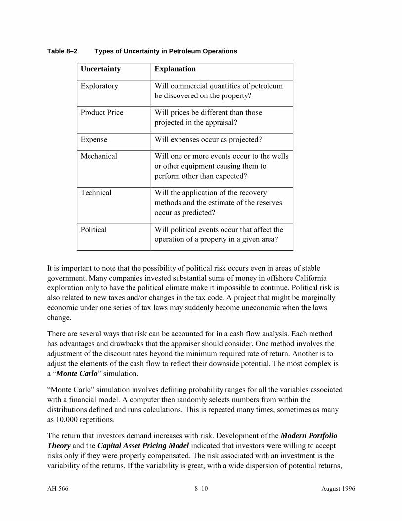
AH 566 8–10 August 1996

Table 8–2 Types of Uncertainty in Petroleum Operations

Uncertainty Explanation

Exploratory Will commercial quantities of petroleum be discovered on the property?

Product Price Will prices be different than those projected in the appraisal?

Expense Will expenses occur as projected?

Mechanical Will one or more events occur to the wells or other equipment causing them to perform other than expected?

Technical Will the application of the recovery methods and the estimate of the reserves occur as predicted?

Political Will political events occur that affect the operation of a property in a given area?

It is important to note that the possibility of political risk occurs even in areas of stable government. Many companies invested substantial sums of money in offshore California exploration only to have the political climate make it impossible to continue. Political risk is also related to new taxes and/or changes in the tax code. A project that might be marginally economic under one series of tax laws may suddenly become uneconomic when the laws change.

There are several ways that risk can be accounted for in a cash flow analysis. Each method has advantages and drawbacks that the appraiser should consider. One method involves the adjustment of the discount rates beyond the minimum required rate of return. Another is to adjust the elements of the cash flow to reflect their downside potential. The most complex is a “Monte Carlo” simulation.

“Monte Carlo” simulation involves defining probability ranges for all the variables associated with a financial model. A computer then randomly selects numbers from within the distributions defined and runs calculations. This is repeated many times, sometimes as many as 10,000 repetitions.

The return that investors demand increases with risk. Development of the Modern Portfolio Theory and the Capital Asset Pricing Model indicated that investors were willing to accept risks only if they were properly compensated. The risk associated with an investment is the variability of the returns. If the variability is great, with a wide dispersion of potential returns,

AH 566 8–11 August 1996

then the risk is assumed to be great. A narrow dispersion of potential returns lessens the variability and the risk is assumed to be lower.

The two methods available to investors to reduce risk are diversification and reduction of exposure. Diversification involves investing in many projects instead of putting all funds on one project. Reduced exposure involves taking a smaller participation in the project, i.e., a smaller working interest.

For further discussions of risk and uncertainty, see references listed in the bibliography.

Income Multipliers While income multipliers can be a very effective way of appraising some income properties as discussed in AH 501 and 501A, they have limited use for petroleum properties. A unit multiplier is developed from analysis of current sales and is adjusted in conformance with Rules 4 and 8. The analysis required to make sure the numbers being applied come from comparable properties is almost as complex as doing a straightforward cash flow analysis. Quoting from the ninth edition of The Appraisal of Real Estate, “…the unit of comparison selected must be consistently applied to the subject property and all comparable sales properties in each analysis.”3 This required level of consistency is difficult to achieve for petroleum properties because of the uniqueness of each property.

“Rules of Thumb” that many experts in the industry use for quick evaluations of properties are the result of numerous cash flow analyses. They are also used by industry management to determine whether to allocate additional resources for further study. The accuracy of these “Rules” is not sufficient for property tax appraisals.

Measures of Success After the discount rate has been selected and the adjustments for risk made, the appraiser discounts the net operating income of the property to reach a value conclusion.

Several methods are used by industry management to evaluate the fair market value using income information. The most common is to accept a project that provides a positive net present value at a specific discount rate. Other non-discounting methods are sometimes used, such as payout time, profit to investment ratio, and average annual rate of return. The criteria for payout time is the acceptance of projects that will return the original investment within a specific period of time. The profit to investment ratio measures the magnitude of the total profit over the life of the project against the investment required. These methods do not offer a means of valuing the property, but provide a check of the assumptions made to see that they are reasonable and yield results in an acceptable range.

3 The Appraisal of Real Estate, ninth edition, American Institute of Real Estate Appraisers, Chicago, IL., 1987, p.151

AH 566 8–12 August 1996

TAXABLE VALUE

As previously noted, for each year after initial enrollment, the taxable value is the lesser of the property’s current market value or its factored base year value.4 Since petroleum properties are analyzed each year to determine the proper taxable value, Rule 468 provides the framework for determining the factored base year value of proved reserves. Figure 8–1 (following) details the steps required by Rule 468 to arrive at a taxable value for a petroleum property. (This worksheet uses the information from the example at the end of the chapter.)

CURRENT MARKET VALUE The value determined by the cash flow analysis or other acceptable appraisal methods is an estimate of the current market value of the assessable property. This is the estimate of what 100 percent of the property would sell for in the open market on the lien date, meeting every condition of an arms length transaction. All of the risks associated with the property and a satisfactory return to the purchaser should be reflected in the current market value.

To determine the value of the mineral rights, the estimated value of the active improvements (wells and surface equipment) is offset from the total cash flow value. Changes to reserves are quantified based on forecast economics. The value of idle wells and idle surface equipment is added to the cash flow value to arrive at the total fair market value.

FACTORED BASE YEAR VALUE Proposition 13 affects petroleum and other mineral properties similar to the way it affects most real estate in that once a base year value has been established, that value remains in effect, unless certain events occur, such as a change in ownership or new construction. However, as previously discussed in regard to Rule 468 (Chapter 6), there are several factors unique to petroleum properties which require consideration in making the annual calculations for adjusted base year values.

First, since petroleum properties are a wasting asset, some of the reserves that were part of the initial base year value are removed from the ground each year and are no longer part of the mineral estate. The base year value of those reserves must be removed from the total.

Secondly, the quantity of reserves may increase or decrease from year to year depending on both economic conditions and on physical operating conditions. Reserves may increase as a result of increased product prices, reduced operating expenses, results of exploration, or other conditions. These new reserves are taxable and acquire a base year value as of the first lien date they are considered proved. Decreases in reserves as a result of economic conditions or

4 For purposes of this chapter, “factored base year value” includes the compounded base year value of real property as described by subdivision (a) of Section 51 of the Revenue and Taxation Code plus the fair market value of property that is not subject to base year value procedures, such as personal property and real property under construction.

AH 566 8–13 August 1996

engineering information are treated the same way as decreases due to depletion; they are no longer considered proved and their base year values must be removed.

Figure 8–1 demonstrates the steps that must be taken to determine the taxable value of an oil producing property, including a detailed explanation of steps required to calculate the adjusted base year value of the reserves, as demonstrated under “Base Year Value Adjustments.” Also, see Rule 468, subdivision (c)(4)(C) through (c)(4)(F).

The following paragraphs constitute an explanation of the terminology in Figure 8–1.

Prior Year’s Adjusted Base Year Value of Reserves. This is the amount of the adjusted base year value of the reserves on the previous lien date, but not necessarily the prior year’s roll value. If the fair market value on the previous lien date was lower than the adjusted base year value, the fair market value would have been enrolled as the taxable value.

Prior Year’s Adjusted Base Year Value of Removed Reserves. This is the volume of reserves removed for all reasons (depletion, economic conditions, and engineering information) multiplied by the weighted average adjusted base year value of the reserves as of the previous lien date. This number is subtracted from the previous year’s value to yield the Prior Year’s Adjusted Base Year Value of Remaining Reserves.

Quantity of New Reserves — Barrels. This represents the quantity of all new oil reserves. Rule 468 recognizes that during a year, an oil property could have both reserves removed because of depletion and new reserves added due to economic conditions and/or changed physical operating conditions. However, there would not be both removals and additions due to the same cause (such as changing economic conditions). There could be removals during one year, due to economic conditions (or engineering information), followed by additions the following year. The new reserves are multiplied by the Current Market Value of Reserves to arrive at the Value of New Reserves.

The Prior Year’s Adjusted Base Year Value of Remaining Reserves is adjusted by the California Consumer Price Index, not exceeding a 2 percent increase, to arrive at the Current Adjusted Base Year Value of Remaining Reserves. The value of the new reserves is added to arrive at the total Current Adjusted Base Year Value for Reserves.

The other calculations shown in Figure 8–1 follow either fair market value principles or adjusted base year value calculations for conventional properties. The enrolled value is the lesser of the current market value or the adjusted base year value.

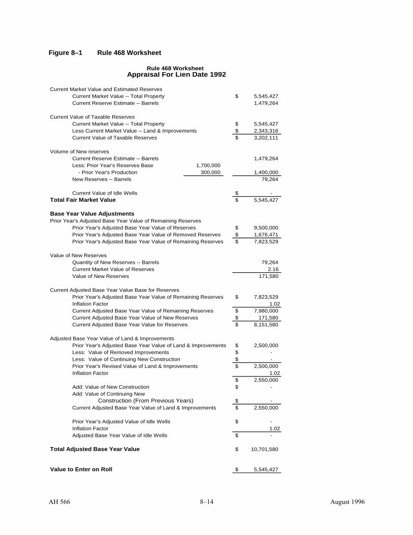
AH 566 8–14 August 1996

Figure 8–1 Rule 468 Worksheet

Rule 468 WorksheetAppraisal For Lien Date 1992

Current Market Value and Estimated ReservesCurrent Market Value -- Total Property 5,545,427$ Current Reserve Estimate -- Barrels 1,479,264

Current Value of Taxable ReservesCurrent Market Value -- Total Property 5,545,427$ Less Current Market Value -- Land & Improvements 2,343,316$ Current Value of Taxable Reserves 3,202,111$

Volume of New reservesCurrent Reserve Estimate -- Barrels 1,479,264 Less: Prior Year's Reserves Base 1,700,000 - Prior Year's Production 300,000 1,400,000 New Reserves -- Barrels 79,264

Current Value of Idle Wells -$ Total Fair Market Value 5,545,427$

Base Year Value AdjustmentsPrior Year's Adjusted Base Year Value of Remaining Reserves

Prior Year's Adjusted Base Year Value of Reserves 9,500,000$ Prior Year's Adjusted Base Year Value of Removed Reserves 1,676,471$ Prior Year's Adjusted Base Year Value of Remaining Reserves 7,823,529$

Value of New ReservesQuantity of New Reserves -- Barrels 79,264 Current Market Value of Reserves 2.16 Value of New Reserves 171,580

Current Adjusted Base Year Value Base for ReservesPrior Year's Adjusted Base Year Value of Remaining Reserves 7,823,529$ Inflation Factor 1.02Current Adjusted Base Year Value of Remaining Reserves 7,980,000$ Current Adjusted Base Year Value of New Reserves 171,580$ Current Adjusted Base Year Value for Reserves 8,151,580$

Adjusted Base Year Value of Land & ImprovementsPrior Year's Adjusted Base Year Value of Land & Improvements 2,500,000$ Less: Value of Removed Improvements -$ Less: Value of Continuing New Construction -$ Prior Year's Revised Value of Land & Improvements 2,500,000$ Inflation Factor 1.02

2,550,000$ Add: Value of New Construction -$ Add: Value of Continuing New

Construction (From Previous Years) -$ Current Adjusted Base Year Value of Land & Improvements 2,550,000$

Prior Year’s Adjusted Value of Idle Wells -$ Inflation Factor 1.02Adjusted Base Year Value of Idle Wells -$

Total Adjusted Base Year Value 10,701,580$

Value to Enter on Roll 5,545,427$

AH 566 8–15 August 1996

Example 8–2

Disclaimer: The following appraisal example is strictly illustrative and is not intended to represent SBE endorsed numbers for the appraisal of a petroleum property. As such, it has no relation to an actual property in California.

AH 566 8–16 August 1996

PROPERTY SUMMARY

Example 8-2

Evaluation Date: January Oil Price: $15.00 Inflation: 3.00% 1995 Gas Price: $2.00 Capitalization Rate: 20.00%

Operator: Board of Equalization NGL Price: $0.75 Exempt Royalty Interest: 0.00% Field: Headquarters Gas/Oil Ratio: 1.00 Non-Exempt Royalty: 12.50%

Lease: Assessment Standards Zone: Minerals

NGL/Gas Ratio: Recovery Method: Primary

1.00 Sinking Fund Rate: 8.0%

Fee Interest Economics Average First Year Production 891 EBPD Economic Life 7

First Year Lifting Costs $5.90 /Bbl Economic Reserves 1,479,264 BOE Total Future Investment $0M Payout @ 10% DR 2.9 years

Payout @ 20% DR 2.3 years

County Tax Rate 1.00% Prop. Taxes/Total 1st Yr Revenue 1.16%

Present Worth and $ / BOE Profile

Discount Rate Fee Interest Economics

PW $ $ / Bbl 10% 6,523,334 4.41 12% 6,301,216 4.26 14% 6,093,621 4.12 16% 5,899,220 3.99 18% 5,716,838 3.86 20% 5,545,427 3.75 22% 5,384,057 3.64 24% 5,231,894 3.54

Fee Interest Economics

7,000,000 6,000,000 5,000,000 4,000,000 3,000,000 2,000,000 1,000,000

0

10.00

8.00

6.00

4.00

2.00

0.00

Discount Rate

PW (M

$)

10%

12%

14%

16%

18%

20%

22%

24%

$ / B

bl

@ 10% @ 20% $/EBPD 7,319 6,222

$/EBR 4.41 3.75

AH 566 8-17 August 1996

Beginning Decline Production: 800.00 BPD

Economic Limit: Remaining Technical Reserves:

10 BPD 1,802,188 BBLS.

Forecasted Production

1000

100

10

1

Example 8-2

DECLINE CURVE ANALYSIS

Decline Rate: 16.00% Decline Start Year: 1995

Decline Start Month: 1

Oil Rate Year End

Decline Crv. Production

Scheduled Production Production

Cumulative Production Remaining Injectant

Year BPD Bbls./Yr Bbls./Yr Bbls./Yr Bbls. Bbls. BOPD Bbls/day 1995 682 270,577 0 270,577 270,577 1,531,611 741 0 1996 581 229,940 0 229,940 500,517 1,301,670 630 0 1997 495 195,942 0 195,942 696,460 1,105,728 537 0 1998 422 166,971 0 166,971 863,431 938,757 457 0 1999 359 142,283 0 142,283 1,005,714 796,474 390 0 2000 306 121,246 0 121,246 1,126,960 675,228 332 0 2001 261 103,319 0 103,319 1,230,279 571,909 283 0 2002 222 88,043 0 88,043 1,318,321 483,866 241 0 2003 190 75,025 0 75,025 1,393,346 408,841 206 0 2004 162 63,932 0 63,932 1,457,278 344,909 175 0 2005 138 54,479 0 54,479 1,511,757 290,430 149 0 2006 117 46,424 0 46,424 1,558,182 244,006 127 0 2007 100 39,560 0 39,560 1,597,742 204,446 108 0 2008 85 33,711 0 33,711 1,631,453 170,735 92 0 2009 73 28,727 0 28,727 1,660,179 142,008 79 0 2010 62 24,479 0 24,479 1,684,658 117,529 67 0 2011 53 20,860 0 20,860 1,705,518 96,670 57 0 2012 45 17,775 0 17,775 1,723,293 78,894 49 0 2013 38 15,147 0 15,147 1,738,441 63,747 41 0 2014 33 12,908 0 12,908 1,751,348 50,839 35 0 2015 28 10,999 0 10,999 1,762,347 39,840 30 0 2016 24 9,373 0 9,373 1,771,720 30,467 26 0 2017 20 7,987 0 7,987 1,779,707 22,480 22 0 2018 17 6,806 0 6,806 1,786,513 15,674 19 0 2019 15 5,800 0 5,800 1,792,313 9,874 16 0

BPD

1995

1996

1997

1998

1999

2000

2001

2002

2003

2004

2005

2006

2007

2008

2009

2010

2011

2012

2013

2014

2015

2016

2017

2018

2019

AH 566 8-18 August 1996

Example 8-2

This page intentionally left blank.

AH 566 8-19 August 1996

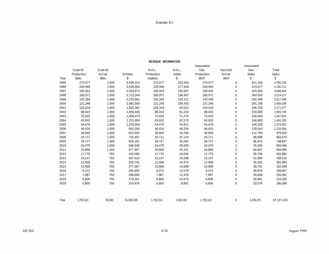
Example 8-2

REVENUE INFORMATION Associated Associated

Crude Oil Crude Oil N.G.L. N.G.L. Gas Gas Used Gas Total Production As Fuel Oil Sales Production Sales Production As Fuel Sales Sales

Year Bbls. Bbls. $ Gallons $ MCF MCF $ $ 1995 270,577 1,500 4,036,153 270,577 202,933 270,577 0 541,154 4,780,239 1996 229,940 1,500 3,529,405 229,940 177,629 229,940 0 473,677 4,180,711 1997 195,942 1,500 3,094,873 195,942 155,937 195,942 0 415,833 3,666,644 1998 166,971 1,500 2,712,346 166,971 136,847 166,971 0 364,924 3,214,117 1999 142,283 1,500 2,376,892 142,283 120,111 142,283 0 320,296 2,817,298 2000 121,246 1,500 2,082,580 121,246 105,433 121,246 0 281,156 2,469,169 2001 103,319 1,000 1,832,361 103,319 92,513 103,319 0 246,703 2,171,577 2002 88,043 1,000 1,605,935 88,043 81,219 88,043 0 216,585 1,903,739 2003 75,025 1,000 1,406,473 75,025 71,274 75,025 0 190,063 1,667,810 2004 63,932 1,000 1,231,894 63,932 62,573 63,932 0 166,863 1,461,330 2005 54,479 1,000 1,078,053 54,479 54,911 54,479 0 146,428 1,279,392 2006 46,424 1,000 943,309 46,424 48,204 46,424 0 128,543 1,120,056 2007 39,560 1,000 824,543 39,560 42,296 39,560 0 112,790 979,629 2008 33,711 1,000 720,457 33,711 37,124 33,711 0 98,998 856,579 2009 28,727 1,000 629,161 28,727 32,593 28,727 0 86,914 748,667 2010 24,479 1,000 548,629 24,479 28,600 24,479 0 76,266 653,494 2011 20,860 1,000 477,957 20,860 25,101 20,860 0 66,937 569,995 2012 17,775 750 422,090 17,775 22,034 17,775 0 58,758 502,882 2013 15,147 750 367,610 15,147 19,338 15,147 0 51,568 438,516 2014 12,908 750 319,746 12,908 16,974 12,908 0 45,263 381,983 2015 10,999 750 277,667 10,999 14,899 10,999 0 39,731 332,298 2016 9,373 750 240,650 9,373 13,079 9,373 0 34,878 288,607 2017 7,987 750 208,005 7,987 11,478 7,987 0 30,608 250,091 2018 6,806 750 179,261 6,806 10,073 6,806 0 26,861 216,195 2019 5,800 750 153,976 5,800 8,842 5,800 0 23,579 186,398

Total 1,792,313 26,000 31,300,025 1,792,313 1,592,016 1,792,313 0 4,245,375 37,137,415

AH 566 8-20 August 1996

Example 8-2

EXPENSE INFORMATION Normal Incremental

# Producing Operating Flood Fuel Gas Capital Other Total Royalty Net Income Wells Expense Expense Expense Expenditures Expenses Costs Payment BFIT

Year $ $ $ $ $ $ $ $ 1995 20 1,920,000 0 0 0 1,920,000 600,342 2,259,897 1996 20 1,977,600 0 0 0 1,977,600 525,486 1,677,625 1997 20 2,036,928 0 0 0 2,036,928 461,315 1,168,401 1998 20 2,098,036 0 0 0 2,098,036 404,838 711,243 1999 20 2,363,569 0 0 0 2,363,569 355,328 98,402 2000 20 2,434,476 0 0 0 2,434,476 311,907 (277,214) 2001 15 1,880,632 0 0 0 1,880,632 273,686 17,259 2002 15 1,937,051 0 0 0 1,937,051 240,274 (273,586) 2003 15 1,995,163 0 0 0 1,995,163 210,851 (538,204) 2004 15 2,055,018 0 0 0 2,055,018 185,113 (778,801) 2005 15 2,298,097 0 0 0 2,298,097 162,444 (1,181,149) 2006 15 2,367,040 0 0 0 2,367,040 142,603 (1,389,587) 2007 15 2,438,051 0 0 0 2,438,051 125,127 (1,583,548) 2008 15 2,511,193 0 0 0 2,511,193 109,825 (1,764,440) 2009 15 2,586,528 0 0 0 2,586,528 96,420 (1,934,281) 2010 15 2,664,124 0 0 0 2,664,124 84,608 (2,095,237) 2011 15 2,182,401 0 0 0 2,182,401 74,258 (1,686,663) 2012 11 2,089,199 0 0 0 2,089,199 65,184 (1,651,502) 2013 11 2,151,875 0 0 0 2,151,875 57,208 (1,770,567) 2014 11 2,216,432 0 0 0 2,216,432 50,213 (1,884,662) 2015 11 2,282,925 0 0 0 2,282,925 44,077 (1,994,704) 2016 11 2,351,412 0 0 0 2,351,412 38,692 (2,101,498) 2017 11 2,421,955 0 0 0 2,421,955 33,956 (2,205,820) 2018 11 2,494,613 0 0 0 2,494,613 29,799 (2,308,218) 2019 11 2,569,452 0 0 0 2,569,452 26,158 (2,409,212)

Total 56,323,770 0 0 0 0 56,323,770 4,709,713 (23,896,067)

AH 566 8-21 August 1996

Example 8-2

Year

FAIR MARKET VALUE INFORMATION Fee Interest

Net Oper. Economic Capitalized Income Production Sinking Fund NOI

$ Bbls. $ $ 1995 2,857,427 325,336 93,674 2,515,439 1996 2,200,214 276,476 93,674 1,580,503 1997 1,626,731 235,597 93,674 937,831 1998 1,113,008 200,763 93,674 494,454 1999 450,564 171,079 93,674 104,729 2000 31,432 145,784 93,674 (82,140) 2001 288,706 124,229 93,674 (5,389) 2002 (35,619) 0 0 0 2003 (329,728) 0 0 0 2004 (596,134) 0 0 0 2005 (1,021,225) 0 0 0 2006 (1,249,580) 0 0 0 2007 (1,461,095) 0 0 0 2008 (1,657,367) 0 0 0 2009 (1,840,698) 0 0 0 2010 (2,013,551) 0 0 0 2011 (1,615,414) 0 0 0 2012 (1,588,641) 0 0 0 2013 (1,715,753) 0 0 0 2014 (1,836,915) 0 0 0 2015 (1,953,166) 0 0 0 2016 (2,065,422) 0 0 0 2017 (2,174,558) 0 0 0 2018 (2,281,193) 0 0 0 2019 (2,385,913) 0 0 0

Total (19,253,890) 1,479,264 5,545,427

AH 566 8-22 August 1996

Example 8-2

PRODUCT PRICE AND COST INFORMATION

Before Inflation Annual Oper. Total Fluid Annual Oper. Other Annual

Oil Price Gas Price N.G.L. Price Costs Capacity Cost Oper. Costs Investment Flood Costs per Bbl. per MCF per Gallon per well Bbl / Year per Barrel Entire Prop. Entire Prop.

1995 15.00 2.00 0.75 24,000 360,000 4.00 0 0 $0 1996 15.45 2.06 0.77 24,000 360,000 4.00 0 0 $0 1997 15.92 2.12 0.80 24,000 360,000 4.00 0 0 $0 1998 16.39 2.19 0.82 24,000 360,000 4.00 0 0 $0 1999 16.88 2.25 0.84 24,000 360,000 4.50 0 0 $0 2000 17.39 2.32 0.87 24,000 360,000 4.50 0 0 $0 2001 17.91 2.39 0.90 24,000 270,000 4.50 0 0 $0 2002 18.45 2.46 0.92 24,000 270,000 4.50 0 0 $0 2003 19.00 2.53 0.95 24,000 270,000 4.50 0 0 $0 2004 19.58 2.61 0.98 24,000 270,000 4.50 0 0 $0 2005 20.16 2.69 1.01 24,000 270,000 5.00 0 0 $0 2006 20.77 2.77 1.04 24,000 270,000 5.00 0 0 $0 2007 21.38 2.85 1.07 24,000 270,000 5.00 0 0 $0 2008 22.03 2.94 1.10 24,000 270,000 5.00 0 0 $0 2009 22.69 3.03 1.13 24,000 270,000 5.00 0 0 $0 2010 23.37 3.12 1.17 24,000 270,000 5.00 0 0 $0 2011 24.07 3.21 1.20 24,000 200,000 5.00 0 0 $0 2012 24.79 3.31 1.24 24,000 200,000 5.00 0 0 $0 2013 25.53 3.40 1.28 24,000 200,000 5.00 0 0 $0 2014 26.30 3.51 1.32 24,000 200,000 5.00 0 0 $0 2015 27.09 3.61 1.35 24,000 200,000 5.00 0 0 $0 2016 27.91 3.72 1.40 24,000 200,000 5.00 0 0 $0 2017 28.74 3.83 1.44 24,000 200,000 5.00 0 0 $0 2018 29.60 3.95 1.48 24,000 200,000 5.00 0 0 $0 2019 30.49 4.07 1.52 24,000 200,000 5.00 0 0 $0

Estimated P&A Cost: Injectant Cost/Bbl:

35,000 0.00

AH 566 8-23 August 1996

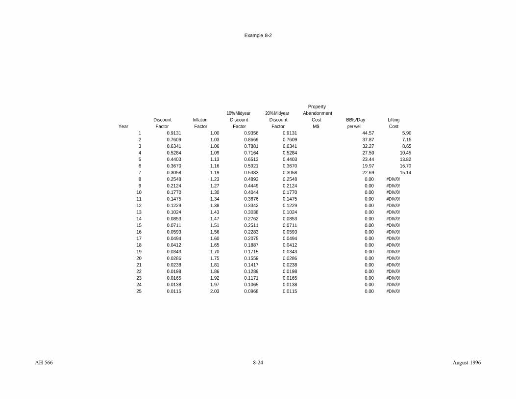
Example 8-2

Property 10% Midyear 20% Midyear Abandonment

Discount Inflation Discount Discount Cost BBls/Day Lifting Year Factor Factor Factor Factor M$ per well Cost

1 0.9131 1.00 0.9356 0.9131 44.57 5.90 2 0.7609 1.03 0.8669 0.7609 37.87 7.15 3 0.6341 1.06 0.7881 0.6341 32.27 8.65 4 0.5284 1.09 0.7164 0.5284 27.50 10.45 5 0.4403 1.13 0.6513 0.4403 23.44 13.82 6 0.3670 1.16 0.5921 0.3670 19.97 16.70 7 0.3058 1.19 0.5383 0.3058 22.69 15.14 8 0.2548 1.23 0.4893 0.2548 0.00 #DIV/0! 9 0.2124 1.27 0.4449 0.2124 0.00 #DIV/0!

10 0.1770 1.30 0.4044 0.1770 0.00 #DIV/0! 11 0.1475 1.34 0.3676 0.1475 0.00 #DIV/0! 12 0.1229 1.38 0.3342 0.1229 0.00 #DIV/0! 13 0.1024 1.43 0.3038 0.1024 0.00 #DIV/0! 14 0.0853 1.47 0.2762 0.0853 0.00 #DIV/0! 15 0.0711 1.51 0.2511 0.0711 0.00 #DIV/0! 16 0.0593 1.56 0.2283 0.0593 0.00 #DIV/0! 17 0.0494 1.60 0.2075 0.0494 0.00 #DIV/0! 18 0.0412 1.65 0.1887 0.0412 0.00 #DIV/0! 19 0.0343 1.70 0.1715 0.0343 0.00 #DIV/0! 20 0.0286 1.75 0.1559 0.0286 0.00 #DIV/0! 21 0.0238 1.81 0.1417 0.0238 0.00 #DIV/0! 22 0.0198 1.86 0.1289 0.0198 0.00 #DIV/0! 23 0.0165 1.92 0.1171 0.0165 0.00 #DIV/0! 24 0.0138 1.97 0.1065 0.0138 0.00 #DIV/0! 25 0.0115 2.03 0.0968 0.0115 0.00 #DIV/0!

AH 566 8-24 August 1996

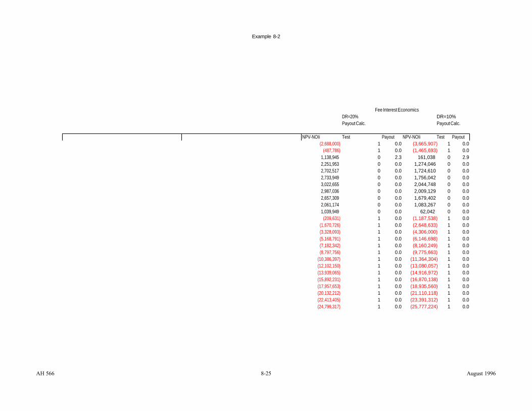
NPV-NOIi Test Payout NPV-NOIi Test Payout

Example 8-2

Fee Interest Economics DR=20% DR=10% Payout Calc. Payout Calc.

(2,688,000) 1 0.0 (3,665,907) 1 0.0 (487,786) 1 0.0 (1,465,693) 1 0.0

1,138,945 0 2.3 161,038 0 2.9 2,251,953 0 0.0 1,274,046 0 0.0 2,702,517 0 0.0 1,724,610 0 0.0 2,733,949 0 0.0 1,756,042 0 0.0 3,022,655 0 0.0 2,044,748 0 0.0 2,987,036 0 0.0 2,009,129 0 0.0 2,657,309 0 0.0 1,679,402 0 0.0 2,061,174 0 0.0 1,083,267 0 0.0 1,039,949 0 0.0 62,042 0 0.0 (209,631) 1 0.0 (1,187,538) 1 0.0

(1,670,726) 1 0.0 (2,648,633) 1 0.0 (3,328,093) 1 0.0 (4,306,000) 1 0.0 (5,168,791) 1 0.0 (6,146,698) 1 0.0 (7,182,342) 1 0.0 (8,160,249) 1 0.0 (8,797,756) 1 0.0 (9,775,663) 1 0.0

(10,386,397) 1 0.0 (11,364,304) 1 0.0 (12,102,150) 1 0.0 (13,080,057) 1 0.0 (13,939,065) 1 0.0 (14,916,972) 1 0.0 (15,892,231) 1 0.0 (16,870,138) 1 0.0 (17,957,653) 1 0.0 (18,935,560) 1 0.0 (20,132,212) 1 0.0 (21,110,118) 1 0.0 (22,413,405) 1 0.0 (23,391,312) 1 0.0 (24,799,317) 1 0.0 (25,777,224) 1 0.0

AH 566 8-25 August 1996

Mineral Rights Adjustments

Sample # Determination of Mineral Rights Value

Property Name Assessment Standards

Year 1995 Total Property Fair Market Value (from Income Approach) $ 5,545,427

# of Active wells 20 Cost of New Well $ 110,000 Remaining reserve Factor 0.16 Active well Value $ 343,316

Suface Facilities $ 2,000,000

Land & Improvement Value (included in income approach Standard $ 2,343,316

Mineral Rights Value $ 3,202,111

#of Idle Wells 0 Value of Idle Well 5000 Remaining Reserve Factor 0.16 Idle Well Value $0

Total Land & Improvement Value (for Tax Roll) Less: Surface Facilities

$ 2,343,316 $(2,000,000)

Land and Imp $ 343,300

AH 566 8-26 August 1996

A–1 August 1996

APPENDIX A: GLOSSARY OF TERMS

Term Definition abandonment costs Expenses related to restoring a property to its original

condition including plugging the well and protecting subsurface water formations.

anticlines A subsurface geological structure in the form of a sine curve or elongated dome, favorable to the accumulation of petroleum.

API gravity The weight per unit volume of crude oil or other liquid hydrocarbons as measured by a system recommended by the American Petroleum Institute. Related to specific gravity.

areal extent The horizontal projection of the reservoir formation, usually expressed in acres.

artificial lift A mechanical means of bringing petroleum to the surface when natural forces (pressure) are insufficient.

associated gas Gas that occurs with oil, either as free gas or in solution.

beam capacity The maximum torque rating for a beam-balanced pumping unit. The beam transfers power from the engine to the pump.

behind-pipe Refers to petroleum reservoirs penetrated by wells but never produced.

brackish water Salt water produced with petroleum.

Capital Asset Pricing Model

CAPM. A financial method of estimating the risk and return associate with a project by using corporations as proxies and using the stock market trades to estimate the required investor returns.

casing Metal pipe, generally cement, in a well to provide stability and integrity to the hole. Used to seal off fluids from the well bore. There may be several strings of casing in a well, one inside the other.

cement (1) Mineral material that fills the spaces between individual grains of sedimentary rock.

(2) Concrete used in a well to hold casing in place and to isolate formations.

completion interval The productive portion of a well, usually indicated by the depth to the perforations.

AH 566 A–2 August 1996

compression The application of pressure to gas to pump it from one location to another in a pipeline.

core analysis The taking of a sample of rock from below the earth’s surface and measuring its properties in a laboratory.

cracking A refining process of breaking down large, heavy molecular hydrocarbon chains into simpler and lighter molecules. Accomplished through the application of heat and pressure.

decline curves A means of reviewing a well or field’s performance or history. An analysis tool for identifying production problems and predicting future performance.

dehydrator system A tank or tower through which gas is run to remove entrained water.

diastrophism The process by which the earth’s surface is reshaped through rock movements and displacements.

economic limit The point at which a well or field no longer is profitable.

effective porosity The percent of the total volume of rock that consists of connecting pores.

enhanced recovery techniques

Methods of crude oil recovery after a well’s original rate of production has diminished.

Environmental compliance costs

Those environmental costs associated with continued operation of the property, i.e., air quality permit fees, wildlife habitat preservation, etc.

exponential A type of decline curve that fits a straight line to the production history on a semi-log plot. The simplest and most commonly used decline analysis.

fluid contacts The depth of the interface between gas and oil or oil and water in a reservoir.

footwall The side beneath an inclined fault.

formation gas factor The volume of gas in the reservoir versus the volume of gas at defined surface conditions. Usually expressed as reservoir cubic feet per standard cubic feet (cu ft/SCF).

formation oil factor The volume in barrels that one stock tank barrel occupies in the formation at reservoir temperature and with the solution gas which can be held in the oil at that pressure.

free water knockout A vessel which allows free (non-emulsified) water to separate from the production stream.

A–3 August 1996

government royalties Payments to the government for the right to extract petroleum from government-owned land. In some cases these are a deductible interest in the property.

hanging wall The wall of a fault located above the surface of a fault.

header The collection point for petroleum gathering lines.

heater treater A vessel that uses the application of heat and chemicals to break down an oil/water emulsion.

heavy oils Crude oil of 20º API gravity or less. Heavy crude is usually high viscosity that doesn’t flow freely at atmospheric temperatures. Light crude flows freely at atmospheric temperature (low viscosity) and has an API gravity in the high 30s and 40s.

height The reservoir formation thickness.

heterogeneities Differing characteristics of a formation.

igneous Rocks that have solidified from a molten state deep in the earth.

immiscible Incapable of mixing, will not dissolve.

interfacial tension The force per unit of length existing at the interface of two immiscible fluids.

irreducible oil saturation The amount of oil in a formation the can not be produced by mechanical means.

kerogen A bituminous material occurring in certain shales that yield a type of oil when heated.

metamorphic Rocks formed by the metamorphosis of other rocks through the application of heat, pressure, and chemical action.

midyear factoring A method of discounting cash flows that assumes the payment is made in the middle of the discounting period.

miscibility Mixable; fluids that are capable of dissolving in one another.

mobility ratio The relative ability of a formation to conduct one type of fluid over another.

Modern Portfolio Theory A financial theory that risk is reduced with proper diversification of assets.

Monte Carlo A method for calculating the probability distribution of possible outcomes, e.g., from a project.

AH 566 A–4 August 1996

net revenue interest A fractional share of a property that represents the income of a property after all costs including taxes, royalties, and other assessments have been paid.

neutron log A tool used by operators to determine the existence of fluid in a reservoir behind well casing.

non-associated gas Free gas; gas not in contact with crude oil in a reservoir.

offset locations A well site drilled on the next location from the original well. The distance between the wells depends upon the spacing regulations.

payout time Recovery from production of the costs of drilling, completing, and equipping a well.

permeability A measure of the resistance of rock to the flow of fluid through it.

petroleum sulfonates A surfactant used for chemical flooding of a reservoir.

pilot study The experimental testing of a recovery method on part of the reservoir.

pinchout The disappearance of a porous, permeable formation between two layers of impervious rock.

plate tectonics A geologic theory that the earth’s surface consists of plates whose constant motion explain continental drift and mountain building.

polyacrylamides A type of polymer injected into a reservoir to block the more permeable channels and direct the injection material into unswept areas of the reservoir

polysaccharides A type of polymer with different properties than a polyacrylamide that allows it use in different types of reservoirs.

porosity The volume of pore space of a rock expressed as a percent of total volume.

primary recovery Production from a reservoir by natural energy that results in flowing wells or wells on a pump with the oil flowing freely into the well bore.

production curves Plots of a well or field’s production versus some other measure such as time or pressure.

profit to investment ratio The total profit from a project divided by the total investment. Ratios greater than one indicate profitable investments.

quitclaimed Relinquishment of a interest in land.

A–5 August 1996

recovery factor The percentage of original oil in place that is extracted from the reservoir.

reserves An estimate of the volume of recoverable petroleum.

royalty interest An interest in minerals produced from a property free of any of the costs of that production; usually paid to the mineral owner in exchange for permission to extract minerals from the property.

secondary recovery The extraction of oil from a field beyond what is capable through the natural energy present in the reservoir, generally through the use of waterflooding, gas injection, or other injection methods.

sedimentary Rock formed by the laying down of material in layers compacted by succeeding deposits.

seeps An occurrence of petroleum on the surface of the earth that is the result of natural forces.

semi-log paper Graphing paper with a log scale on one axis.

separators A pressure vessel used for the purpose of separating well fluids into gaseous and liquid components.

slug A measured amount of fluid injected into a reservoir for enhanced recovery.

specific gravity The ratio between equal volumes of a liquid and water or a gas and air at a standard temperature and pressure where the weight of the water or air is given a value of one.

springs An occurrence of petroleum at the earth’s surface through natural forces.

stimulation Enhancing a wells productive capacity.

surfactant A surface active agent used for enhanced recovery of petroleum.

sweep efficiency The displacement efficiency of a flooding method.

synclines A bowl shaped geological structure usually not favorable to the accumulation of petroleum.

technical reserves Reserves that can be recovered by existing technical methods but that may not be economic. Technical reserves are a subset of the original oil in place of a field. Proved reserves are a subset of technical reserves.

thermal degradation The breaking down of a complex molecular structure through the application of heat.

AH 566 A–6 August 1996

trap rock A geological structure that retards the free migration of petroleum and concentrates it in a limited space.

ultimate recovery The total expected recovery from a field from discovery to abandonment.

viscosity One of the physical properties of a fluid regarding its ability to flow. Higher viscosities are more resistant to flow.

water saturation The amount of water in a formation expressed as a percent of total fluid.

well logs A recording of the properties of a formation measured by electrical, acoustic, and radioactive instruments.

working interest The operating interest of a petroleum property. This interest is subject to all of the costs of drilling, completion, and operation of the property.

workover Operations on a producing well to restore or increase production.

AH 566 B– 1 August 1996

APPENDIX B: SUMMARY OF RELATED COURT CASES

Atlantic Oil Co. v. County of Los Angeles, 69 C.2d 585 (1968), distinguished mines and minerals as real property, in contrast to royalties received through the lease of mineral property. The broad meaning of mines and minerals, “whether or not belonging to the owner of the land in Section 104(b), is the right to enter the land for the production of oil and gas:

The right to receive royalties is an interest in oil and gas when they are removed from the land and reduced to possession.

Callahan v. Martin, 3 Cal.2d 110, 128, (1935) The person who has the right to enter upon the land to drill for oil and gas and to retain as his property all substances brought to the surface, has an interest or estate in real property in the nature of a profit a prendre.

California Portland Cement Co. v. State Bd. of Equalization 67 Cal.2d 578 (1967). The capitalization of income approach is a generally accepted method of valuing mineral [oil and gas properties], and has been expressly approved by the California Supreme Court.

Carlson v. Assessment Appeals Bd. I, 167 Cal.App.3d 1004 (1985) In determining the fair market value of the property per Section 110, the assessor is required to consider under Section 402.1 only governmentally imposed land restrictions necessary to implement public policy, not restrictions for the benefit of private parties.

Chanslor-Western Oil & Dev. Co. v. Cook 101 Cal.App.3d 407 (1980) The assessor, in defending his assessment of a competitor’s property, could not introduce details of property acquisition transactions acquired from the assessee under Section 408.

Clayton v. County of Los Angeles, 26 Cal.App.3d 390 (1972) Fair market value properly reflects economic rent rather than mere contract rent.

Dennis v. County of Santa Clara, 215 Cal.App.3d 1019 (1989) Proper application of Rule 2(a) means that the real property being appraised must be appraised as though it were unencumbered or unrestricted by a lease, mortgage, or other private agreement, even though it may, in fact, be so encumbered. Firestone Tire & Rubber Co. v. County of Monterey (1990) 223 Cal.App.3d 382, did not apply Section 402.1 in finding that toxic waste cleanup costs must be considered in determining the value of the property. However, per Section 110, where the cost of pollution cleanup reduces the fair market value of property, it may form the basis for a reduction in that property’s assessed valuation.

Freeport-McMoran Resource Partners v. County of Lake, (1993) 12 Cal.App.4th 634. In calculating the income stream for certain geothermal power plants, the assessor properly capitalized the plants’ income from fixed priced commodity contracts (under which site-specific plants sold electricity to a power company at rates far above market price,. the “full value” of the plants included projected income at the (SO4) contract rate, rather than the

AH 566 B–2 August 1996

market rate, since a prospective buyer would be willing to pay more for the plants with the SO4 contracts.

Howard v. County of Amador, 220 Cal.App.3d 962 (1990), the surrender of certain mineral rights through the assignment of a mineral sublease was, in effect, “the conveyance of a mineral interest in land,” and a change of ownership (per Section 60) and reassessment of the mineral rights (fee) being transferred.

Lynch v. State Board of Equalization, 64 Cal.App.3d 94 (1985), the provisions of Proposition 13 (Article XIII A of the California Constitution) apply to oil and gas producing properties. Rejecting the pre-Proposition 13 method of annual reassessment of oil and gas interests, the court stated that when the voters enacted an acquisition system of taxation under Proposition 13, it became necessary to define more clearly the nature of the taxable interest in oil and gas property, and that Property Tax Rule 468 was the means of accomplishing this.

Main & Von Karman Associates v. County of Orange 23 Cal.App.4th 337 (1994) Holds that the appeals board improperly based its value determination under Rule 4 on “comparable sales data” that was not adjusted to reflect the differences between the subject property and the comparison properties as required.

Oryx Energy Company v. County of Kern, 17 Cal.App.4th 48 (1993) held that the assessor properly assessed a taxable possessory interest in federal land under certain pre-DeLuz oil and gas leases by including the government royalty interest in the valuation, in accordance with Section 107.2, on the ground that the leases had been extended under terms which did not prohibit a reduction in the royalty rate.

Phillips Petroleum Co. v. County of Lake, 15 Cal.App.4th 180 (1993), held that Rule 468(c)(6) approaches the taxation of oil and gas interests in terms of an “appraisal unit,” consisting of four components: (1) proved reserves; (2) wells, casings, and parts thereof; (3) land (other than mineral interests); and (4) improvements.

Roberts v. Gulf Oil Corporation (1983) 147 Cal.App.3d 770, 796 concluded that the county assessor has authority under Section 441 et seq. to require the disclosure of factual and interpretative information concerning oil and gas properties, providing that “the inquiry is within the authority of the agency, the demand is not too indefinite, and the information sought is reasonably relevant” to the discovery and valuation of taxable property. See also Union Pacific R.R. Co. v. SBE (1989) 49 Cal.3d 138, 146, 150, and Western Oil & Gas Assn. v. SBE (1987) 44 Cal.3d 208, 213-214.

Shafer v. State Board of Equalization, 174 Cal.App.3d 423. The supplemental assessment provisions of Section 75.18, implementing Article XIII A, Section 2(b), do not constitute an ad valorem tax increase.

Tenneco West, Inc. v. County of Kern, 194 Cal.App.3d 596 (1987) held that the subsurface use of property, whether the right to store property (gas) in or upon property, or the right to

AH 566 B– 3 August 1996

enter upon the property and to produce and remove oil and gas, constitutes a taxable real property interest.

AH 566 C–1 August 1996

APPENDIX C: DERIVATION AND ESTIMATION OF DISCOUNT RATES USED IN DISCOUNTED CASH

FLOW ANALYSIS

DISCLAIMER: This appendix represents an introduction to the topic of determining discount rates with the Capital Asset Pricing Model. This appendix does not discuss all of the complexities of the model and the precautions that should be taken regarding its application.

INTRODUCTION This appendix includes a very brief overview of discounted cash flow (DCF) analysis and discusses methods for deriving or estimating the discount rate to be used in the DCF format in the context of property tax valuation and assessment. Three methods of discount rate estimation are discussed: (1) rate derivation from market sales data; (2) surveys of market participants; and (3) use of the band of investment or weighted average cost of capital (WACC).

PRESENT VALUE AND DISCOUNTED CASH FLOW ANALYSIS The Concept of Present Value The concept of present value is one of the most important ideas in valuation. Because investors prefer immediate cash returns over future cash flows, they “discount” future flows, or reduce their value, when analyzing investments. Because of the pure time value of money, this is true even if no risk is involved. A rational investor would not pay $1000 today for the certain right to receive $1000 one year hence, because he or she could earn interest on $1000 in hand, and the total value would accumulate (at the risk-free rate of interest) to an amount greater than $1000 at the end of one year. Thus, to the rational investor, a certain payment of $1000 a year from today is worth something less than $1000 today, with the amount of the discount being determined by the risk-free rate of interest.

Theoretically, the risk-free rate consists of a component for the cost of borrowing money plus a component for anticipated future inflation. It is virtually impossible to identify those components separately, but fortunately there is no need to do so, since the risk-free rate can be established and is the least controversial component in discounted cash flow analysis.

Most investments also involve risk; the returns are variable, not certain. In addition to the pure time value of money (the risk-free rate, which includes an inflation component), the discount rate for risky investments includes a premium for risk.

Discounted Cash Flow Analysis Most investments produce a series of payments over future time periods; a typical pattern is periodic payments (monthly, quarterly, annually) and perhaps a reversionary payment at the end of the investment horizon or holding period. Discounted cash flow (DCF) analysis is a method by which investors explicitly value future cash flows—typically annual cash flows—

AH 566 C–2 August 1996

over an anticipated holding period. In the DCF analysis, anticipated annual cash flows are discounted—typically with the aid of financial tables (for example, Assessors’ Handbook Section 505) or computer software—to their present values. The present values are then summed to obtain an estimate of the market value of the property.

Risk is incorporated into DCF analysis through the discount rate, which includes components for the pure time value of money, inflation, and risk. The discount rate reflects the opportunity cost of the funds used in the investment, the return that could have been earned by investing the funds in an alternative investment opportunity of comparable risk. Accurate estimates of anticipated cash flows and the prudent selection of the discount rate are critical to DCF analysis, which is depicted in equation form below:

PVCF1 r

CF(1 r)

CF(1 r)

CF(1 r)

CF(1 r)

1 22

33

TT

tt

t 1

T

=+

++

++

+ ⋅ ⋅ ⋅ ++

=+=

∑ C– 1

where, PV = the present value, or estimated market value CFt = the cash flow at time t r = the discount rate, reflecting the time value of money, inflation, and risk

In a real estate appraisal context, discounted cash flow analysis is a form of yield capitalization and has been defined as:

“The procedure in which a discount rate is applied to a set of projected income streams and a reversion. The analyst specifies the quantity, variability, timing, and duration of the income streams as well as the quantity and timing of the reversion and discounts each to its present value at a specified yield rate. DCF analysis can be applied with any yield capitalization technique and may be performed on either a lease-by-lease or aggregate basis.” (Appraisal Institute, 1993, p. 102)

Although Property Tax Rule 8 does not specifically mention the DCF method of valuation, it is entirely consistent with it. Subdivision (b), states, in relevant part:

“Using the income approach, an appraiser values an income property by computing the present worth of a future income stream. This present worth depends upon the size, shape, and duration of the estimated stream and upon the capitalization rate at which future income is discounted to its present worth. Ideally, the income steam is divided into annual segments and the present worth of the total income stream is the algebraic sum (negative items subtracted from positive items) of the present worths of the several segments.”

AH 566 C–3 August 1996

Terminology The following concepts are used in this appendix and it is important to define them at the outset. Rates of return, in particular, have many pseudonyms.

Capitalization rate. “Any rate used to convert income into value.” (Appraisal Institute, 1993, p. 48)

Yield rate. “A rate of return on capital, usually expressed as compound annual percentage rate. A yield rate considers all expected property benefits, including the proceeds from sale at the termination of the investment. Yield rates include the interest rate, discount rate, internal rate of return (IRR), overall yield rate (Y O), and equity yield rate (Y E ).)” (Appraisal Institute, 1993, p. 398) A yield rate can apply to the total property—that is both debt and equity—or to only the equity portion.

Discount rate. “A yield rate used to convert future payments or receipts into present value.” (Appraisal Institute, 1993, p.102)

Internal rate of return (IRR). The discount or yield rate which equates the present value of anticipated cash inflows to the present value of cash outflows or costs. It is the rate at which the present value of an investment’s cash inflows equals the cost or price of the investment. The yield to maturity of a bond is an example of an internal rate of return; it is the rate which equates the present value of the future payments on the bond to the current price on the bond.

Cost of capital. The expected return that is foregone by the firm when investing in a project rather than in comparable financial securities in the capital markets. (Brealey and Myers, Fourth Edition, pg. G8). From the firm’s perspective, it is the discount rate used to reduce anticipated cash flows to an estimate of present value. From the investor’s perspective, it is the expected or required rate of return from a debt or equity investment in the firm. The cost of capital reflects a return on the total property; that is, both debt and equity. The band of investment or weighted average cost of capital technique explicitly weights the costs of debt and equity components to arrive an average cost of total capital for a project or investment.

Cost of equity capital. The required return on the company’s common stock in capital markets. It is also called the equityholder’s required rate of return, because it is what equityholders can expect to obtain in the capital markets. It is a cost from the firm’s perspective. (Ross & Westerfield, 1988, p. 830)

Cost of debt capital. The required return on the company’s long-term, permanent debt; the debt holder’s required rate of return. It is a cost from the firm’s perspective.

Required rate of return. The minimum expected rate of return on investment that an investor will accept in order to select an investment.

Expected rate of return. The average of possible returns from an investment weighted by their respective probabilities; the return expected by the investor.

AH 566 C–4 August 1996

Risk. Uncertainty about the outcome of future events. Uncertainty about the future profitability of investments or projects. In finance, risk is quantified using statistical measures of variation. (Brigham and Gapenski, 1988, p. 36)

DERIVING DISCOUNT RATES FROM SALES DATA Introduction The market derived method, the preferred method under Rule 8, is the most direct method of estimating a discount or yield rate, as it extracts it from an actual sales transaction. This method requires detailed information from the buyer. For large properties, particularly those involving investment fiduciaries (for example, pension funds, insurance companies), or purchases involving natural resource properties (for example, oil, gas, or mining), detailed pro-forma data reflecting buyer/investor expectations is often available. For smaller transactions, the information may be more difficult to obtain.

To extract a discount rate from a sale, the analyst must: (1) determine that the sales price indicates fair market value, obtain the cash equivalent sales price, and the size of the interest sold; (2) obtain the anticipated income and expenses (the anticipated cash flows) of the buyer; that is, the economic basis on which the buyer purchased the property; (3) convert the buyer’s anticipated income and expense data into a format consistent with Property Tax Rule 8, if necessary; and (4) compute the internal rate of return (IRR) or discount rate based on the sales price and the anticipated net operating income or cash flow.

Sales Data The sales from which discount rates are derived must meet the requirements of market value and cash equivalency as set forth in Property Tax Rule 2, “The Value Concept.” A determination should be made of whether the fee interest or a partial interest was sold.

Anticipated Income and Expenses and Cash Flow Projections The analyst must obtain detailed income and expense projections for the sale being analyzed. These projections must be the buyer’s expectations in order for the derived discount rate to have validity. In many cases, especially for large properties, the buyer’s economic evaluation or pro forma will be available. The level of income from which the discount rate is derived must be carefully defined. Although this appendix does not deal with the valuation phase, the importance of applying the derived rate to the correct level of income when valuing a property is crucial.

Property Tax Rule 8, subdivision (c) refers to the proper income to be capitalized and not the income from which a rate is to be derived. Nevertheless, the requirements of Rule 8(c) are informative and useful for purposes of deriving a capitalization rate. Rule 8(c) reads:

“The amount to be capitalized is the net return which a reasonably well informed owner and reasonably well informed buyers may anticipate on the valuation date…. Net return, in this context, is the difference

AH 566 C–5 August 1996

between gross return and gross outgo. Gross return means any money or money’s worth which the property will yield over and above vacancy and collection losses, including ordinary income, return of capital, and the total proceeds from sales of all or part of the property. Gross outgo means any outlay of money or money’s worth, including current expenses and capital expenditures (or annual allowances therefor) required to develop and maintain the estimated income. Gross outgo does not include amortization, depreciation, or depletion charges, debt retirement, interest on funds invested in the property, or rents and royalties payable by the assessee for use of the property. Property taxes, corporation net income taxes, and corporation franchise taxes measured by net income are also excluded from gross outgo.”

When deriving a rate for assessment purposes, the income is identical to that described above, with the exception of the treatment of anticipated property taxes, which are deducted from income when deriving a discount rate but remain in the income stream when capitalizing an income stream into an estimate of value. The income from which the discount rate is derived is the anticipated net income before investment recapture (NIBR), also known as the anticipated net operating income (NOI). It is the anticipated net operating cash flow that remains after all anticipated cash operating expenses, including anticipated property taxes, are deducted from anticipated cash revenue. Financing costs, accounting depreciation charges, and federal and state income taxes are not deducted from the income steam. There may also be a reversionary cash flow at the end of the holding period, which is a cash flow from the sale of the property or asset, less disposition costs at the end of the investment horizon. The income data provided by the buyer may have to be “reconstructed” to the above format, and for specialized property types this framework may not coincide with industry convention. In general, to derive a discount rate, the income data supplied by the buyer should be converted to an annual anticipated net operating income on a cash flow basis, including anticipated property taxes as an expense, but excluding any financing expenses, accounting depreciation charges, and, of course, federal and state income taxes.

Treatment of Inflation in Cash Flows Most forecasts of anticipated income and expenses in DCF analysis build inflation estimates into each element in the income or cash flow statement; the forecasts reflect the impact of anticipated inflation. In economic terms, the forecasts are made on a “nominal” basis. For example, if revenues are expected to increase 5 percent a year over the holding period, reflecting inflation and supply and demand factors, the income estimates for each year in the DCF analysis reflect these anticipated changes.

The discount rates derived from such forecasts are also nominal ones; they contain an inflation component. Although it is possible to estimate both income and hence the discount rate net of inflation—on a real not nominal basis—it is not common practice and requires additional calculations.

AH 566 C–6 August 1996

In the petroleum industry, future anticipated changes in revenues and expenses are commonly referred to as “escalation.” In principal, there is or should be no difference between inflation and escalation, since each term represents the market’s perception of future changes in revenues and expenses. However, the word inflation implies that revenues and expenses are likely to change in accordance with cost-of-living indexes or similar indexes. The word escalation implies that a forecast of changes in revenues and expenses for a specific industry can be made, and those changes may be very different from the more general indexes.

For example, assume that the annual rate of inflation will be 3 percent per year for the foreseeable future. However, the oil industry believes that there will be an oversupply of oil for the next two years resulting in a 20 percent decrease in price, a return to the current price for the following three years, and a severe shortage of oil three-to-five years thereafter, resulting in a 30 percent increase over the current price. Given no other data, buyers (and sellers) would assume that prices for oil (and therefore revenues) will literally decrease for the next two years, will return to the current level for the following three-to-five years, and will increase sharply thereafter. Costs will increase by 3 percent annually.

It should be noted that an escalation rate for oil may be the same as the escalation rate for natural gas, but if that happens, it is only a coincidence. In addition, individual buyers often use different escalation rates, some lenders use different escalation rates than others, and industrywide escalation rates sometimes change dramatically over short periods of time. Understanding escalation is absolutely critical both for deriving capitalization rates and for estimating the future cash flows of a property being appraised.

Computation of the IRR or Discount Rate The final step is to calculate or compute the discount rate for the sale (with aid of a financial calculator or spreadsheet software). The rate derived is the total property yield rate, or IRR, the rate at which the present value of the forecast NIBR or NOI equals the sale price. It is a return on the total property, both debt and equity. The market-derived discount rate reflects the return expectations of market participants and can be used to discount income streams of comparable risk when valuing comparable properties.

CHECKING THE VALIDITY OF DISCOUNT RATES USING MARKET SURVEYS While the use of market surveys is not discussed in the California statutes or the Property Tax Rules, published and unpublished surveys of market participants and analysts can be used as sources of discount rate information. This approach might be called, “Ask someone who knows or should know.” Many studies and surveys are published across many property markets, which provide data regarding expected discount rates. They often present a range of rates. Sources include real estate investment fiduciaries, trade organizations, academic studies, and various industry groups. The appraiser should discover the sources of survey data relevant to the type of property he or she is valuing. The Society of Petroleum Evaluation Engineers publishes an annual survey with discount rates relating to petroleum properties.

AH 566 C–7 August 1996

When using this type of data, both the discount rate and the level of income on which it is based be clearly defined and understood by the analyst. It is common to see an internal rate of return or total property yield rate based upon the property’s NOI, as described the preceding section.

DERIVING DISCOUNT RATES USING THE BAND OF INVESTMENT OR WEIGHTED AVERAGE COST OF CAPITAL

Band of Investment or Weighted Average Cost of Capital Defined The band of investment has been described as “A technique in which the capitalization rates attributable to components of a capital investment are weighted and combined to derive a weighted-average rate attributable to the total investment.” (Appraisal Institute, 1993, p.27) In the band of investment technique, a weighted average is taken of the debt and equity components of capital in order to derive a capitalization rate which can be applied to the total property—both debt and equity.

Property Tax Rule 8 (g) (2) refers to the band of investment, stating that a capitalization rate—that is, any rate used to convert income into value— may be estimated:

“By deriving a weighted average of the capitalization rates for debt and for equity capital appropriate to the California money markets (the band of investment method) and adding increments for expenses that are excluded from outgo because they are based on the value that is being sought or the income that is being capitalized. The appraiser shall weight the rates for debt and equity capital by the respective amounts of such capital he deems most likely to be employed by prospective purchasers.”

The band of investment method is analogous to the WACC technique. In the appraisal literature, the band of investment technique is used to derive an overall capitalization rate to be used with the direct capitalization method of valuation. However, it may be used to derive a yield rate to be used with the yield capitalization method of valuation. The WACC approach also derives a yield or discount rate which can be used in the DCF analysis.

The WACC technique is typically used by publicly-traded corporations to estimate the average cost of capital for the firm’s proposed projects or investments. The WACC is the discount rate which a firm uses to value the cash flows of proposed projects or investments of average risk to the firm. This method uses financial data from the capital markets to estimate a discount rate that can be used in DCF analysis.

The WACC can be thought of as what the firm expects to pay out to debtholders and equityholders for every dollar of capital that it receives from them, or, conversely, what equity and debt investors require from the firm in order to fund or invest in it. The cost of capital is the average cost of the various types of capital the firm uses to fund its assets, with

AH 566 C–8 August 1996

the average weighted by the current market values of the existing permanent financing components— most often long-term debt, preferred stock, and common stock.

The WACC is an opportunity cost. When evaluating projects or proposed investments, a firm asks the question: “Does this project or investment provide a rate of return at least equal to what could be obtained in the capital markets?” The firm’s WACC is the minimum rate of return that the firm must earn on an investment of average risk, an investment with risk comparable to the firm’s existing line of business.

Estimating Capital Structure Weights The cost of capital is a weighted average based on the proportions of total capital—the funds required for the investment—financed by the debt and equity components. The weights should be based on current market values, not book values. The market value of equity is typically quite different from the book or accounting value, and the same is generally true, for debt. In addition, only the permanent components of the financing mix—those used to finance long-term projects or investments—are included in the calculation of the average cost of capital. Typically, these are limited to long-term debt and equity.

Estimating the Cost of Debt The current cost of debt for the project is estimated by using the current yield-to-maturity of long-term debt for the prospective purchasers; the objective is to estimate the current rate at which the prospective purchasers could borrow. This information can be obtained from various financial publications.

CAPM Overview The CAPM is a financial/economic model which is used to estimate an equity rate of return on a given security or portfolio of securities. The CAPM postulates an explicit relationship between the risk of a security (as measured by its “systematic” risk, discussed below) and its expected return. The model concentrates on the estimate of security returns. To estimate the cost of equity using the CAPM, the analyst first estimates the risk of the asset or project being valued using the beta measurement (also discussed below), then converts this risk to the required return or cost of equity using the model. The CAPM estimates an after-tax cost of equity. Since we are estimating a before-tax WACC, we must convert the estimated cost of equity from the CAPM to a before-tax basis.

Portfolio theory is a major component of modern financial theories in general and of the CAPM in particular. Portfolio theory holds that risk can be reduced by combining individual risky assets (real or financial assets) into portfolios rather than holding them individually. (“Don’t put all your eggs in one basket.”) The same level of expected return can be obtained at lower risk by diversifying; in order to obtain the highest expected return for a given level of risk, rational investors should hold portfolios of assets and not individual assets in isolation.

AH 566 C–9 August 1996

The history of capital market returns indicates that risk has been rewarded. Assets of greater risk have produced higher average returns. For example, over the period 1926 to 1994, the average annual return (compound) on U.S. common stocks (large company) was 10.2 percent with a standard deviation of returns of 20.3 percent; for long-term U. S. government bonds the average annual return (compound) was 4.8 percent with a standard deviation of 8.8 percent. Stocks were riskier, on average, but also produced higher average returns (Ibbotson Associates, 1995, p., 33).

The CAPM estimates risk and return in a portfolio context. The model separates the total risk of an individual asset into two components: systematic (market) risk and unsystematic (unique) risk. Systematic risk is the tendency for returns on all assets to move up or down with shifts in the general economy. It is the risk that stems from general macroeconomic forces affecting all investments. Returns on almost all assets are positively correlated with general market movements, although the degree of correlation differs.

Unsystematic risk, by contrast, is the risk that affects a single asset or a small number of assets. A costly labor dispute is an example of unsystematic risk. It affects one company, or perhaps an industry group, but not the entire economy. Building on portfolio theory, the CAPM postulates that in a diversified portfolio, unsystematic risk is eliminated; the effects of unique events affecting individual stocks tend to cancel each other out when assets are held in a portfolio.

The systematic risk in a portfolio cannot be eliminated by diversification. Thus, in a portfolio context, the relevant risk is systematic risk, and expected returns should reflect only the systematic risk and not the total or stand-alone risk of an individual asset. Since rational investors will hold portfolios of assets and not individual assets, the relevant risk of an individual asset should be the risk it contributes to a diversified portfolio, not the asset’s individual or stand-alone risk.

The relevant risk is systematic risk. Furthermore, assets should be valued based upon their systematic risk and the asset’s risk premium—the additional return for making a risky investment rather than a safe or risk-free one. The pure-play approach assumes that the systematic risk for a particular line of business is constant for all firms that compete in that line of business. This means that the beta of the pure-play firm or an average beta of several pure-play firms can be used to estimate the systematic risk of the project under review.

The beta of a security or project is the measure of systematic risk of a security or project. Beta measures the sensitivity of returns to general market movements. A beta of 1.0 indicates a risk level as risky as the market as a whole; an investment with a beta of 1.0 is expected to provide returns to investors equal to those of the market as a whole. A beta of 2.0 indicates a risk level twice that of the market as a whole ; a security with a beta of 2.0 should, on average, rise twice as much as the general market during periods of rising stock prices, and it should fall approximately twice as much as the market in periods of declining stock prices. A beta of 0.5 indicates a risk level one-half that of the market as a whole; a stock with a beta 0.5

AH 566 C–10 August 1996

should rise one-half as much as the general market during rising prices and fall one-half as much during declining prices.

What is the meaning of the “market as a whole,” or the “general market” in the CAPM context? The CAPM conceptualizes the general market or the market as a whole as the “market portfolio.” The market portfolio is a theoretical portfolio of all possible investments, including securities, real estate, plant and equipment, and even investments in human capital. In theory, systematic risk should be measured against a market portfolio containing all possible investments, but such a portfolio does not exist. In practice, for the purpose of measurement, the market portfolio is proxied by a large, diversified stock index.

The CAPM specifies that the size of the expected risk premium is a linear function of the risk of the asset, as measured by its beta. The expected return on equity or cost of equity of a security or asset is the sum of the risk-free rate of return and the product of beta, the relative risk measure, and the market risk premium or compensation for bearing risk. This is represented by the following equation:

r r b (r r )i f i m f= + − C– 2

where, ri = the expected after-tax equity return on security i; the after-tax cost equity rf = the risk-free rate b i = beta, the volatility of security i relative to the market as a whole

(r r )m f− = the market premium, the expected return on the market portfolio above the risk-fee rate

A Few of the Difficulties in Applying CAPM The concept is based on an economic theory with little if any information on how to apply the concept to deriving an equity yield rate for specific real property. The problems include but are not limited to: estimating the risk of an asset using the beta measurement; converting the estimated cost of equity to a before-tax basis; the concept is based on the securities market; deriving an equity risk premium from securities data; and adjusting the derived equity rate to be property specific. In addition to the lack of information on how to apply the concept, the literature on the subject is controversial.

CONCLUSION AND SUMMARY Market-Derived Discount Rates As previously noted, discount rates properly derived from actual sales transactions provide the most direct and supportable market indication of expected discount rates for properties of comparable risk. The market-derived method, preferred under Rule 8, however, requires detailed data regarding the anticipated income and expenses—(cash flows)—of the buyer over the anticipated holding period, and the data must be consistently processed by analysts in order to preserve comparability.

AH 566 C–11 August 1996

Market Surveys A well-prepared and targeted market survey can be an authoritative source of discount rate information. In a good survey, the return measure is precisely defined for survey participants and is the one commonly used by market participants in their market evaluations. The best survey data is often collected by and from institutional investors and fiduciaries. Since these investors are almost exclusively interested in higher-tier properties, the survey method is most applicable to large, investment-grade properties (office buildings, hotels, shopping centers). Good survey data may not be available for property below this tier. Industry groups concerned with specialized property types (resource properties such as oil, gas, railroads, etc.,) may also be good sources of data regarding expected returns for such specialized properties. A strength of the survey approach is that survey data is truly expectational: it asks analysts and market participants what rate of return they expect, and is precisely the type of information that property analysts and appraisers are seeking. A weakness of the method is that it is obviously one step removed from actual market transactions and hence less authoritative than the market-derived method.

Band of Investment or Weighted Average Cost of Capital The band of investment technique is a weighted average of the debt and equity components of capital and is used to derive a capitalization rate. The technique is one of the methods discussed in Property Tax Rule 8.

The WACC technique to derive a capitalization rate is different in name only. Typically the Band of Investment technique is used to derive a direct capitalization rate whereas the WACC technique is used to derive a discount rate.

AH 566 C–12 August 1996

References

Appraisal Institute. The Appraisal of Real Estate (10th ed.). Chicago.

Appraisal Institute. (1993). The Dictionary of Real Estate Appraisal (3rd ed.). Chicago.

Brealey, R. & Myers, S. (1991). Principles of Corporate Finance (4th ed.). New York: McGraw-Hill Book Company.

Brigham, E. F. & Gapenski, L. C. (1993). Intermediate Financial Management (4th ed.). Fort Worth: Harcourt Brace College Publishers.

Ehrhardt, M. C. (1994). The Search for Value: Measuring the Company’s Cost of Capital. Boston: Harvard Business School Press.

Ibbotson Associates. (1995). Stocks, Bonds, Bills, and Inflation: 1995 Yearbook. Chicago.

Richard J. Miller & Associates. Analysis of Oil and Gas Property Transfer and Sales and Derivation of a Band of Investment: 1983 through 1995. (1996). Huntington Beach, CA.

Ross, S. A. & Westerfield, R. W. (1988). Corporate Finance. St. Louis: Times Mirror/Mosby College Publishing.

State of Texas Comptroller of Public Accounts, Property Tax Division. (1994) . Manual for Discounting Oil and Gas Income. Austin, Texas.

Standard & Poor’s Corporation. (Monthly) Standard & Poor’s Bond Guide. New York.

Standard & Poor’s Corporation. (Periodic). Standard & Poor’s Stock Reports New York.

Value Line Publishing,. (Periodic). The Value Line Investment Survey, Part 3 Ratings and Reports. New York.

APPENDIX D: INFLATION TRENDS

20

15

10

5

0

-5

-10

-15 1926 1931 1936 1941 1946 1951 1956 1961 1966 1971 1976 1981 1986 1991

B

B B

B

B B B

B B B B

B

B

B

B

B

B

B B

B

B

B B

B B B B B

B B B

B B B B B B

B B B

BB B B B

BB B B B

B B B

B

B B B B

B

B B

B

B B

Annual Rate of Inflation

B

B B B

B

Infla

tion

Rat

e

AH 566 August 1996 D–1

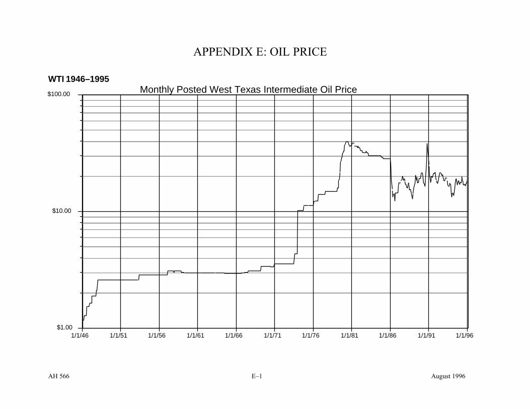
APPENDIX E: OIL PRICE

WTI 1946–1995 $100.00

$10.00

$1.00 1/1/46 1/1/51 1/1/56 1/1/61 1/1/66 1/1/71 1/1/76 1/1/81 1/1/86 1/1/91 1/1/96

Monthly Posted West Texas Intermediate Oil Price

AH 566 E–1 August 1996

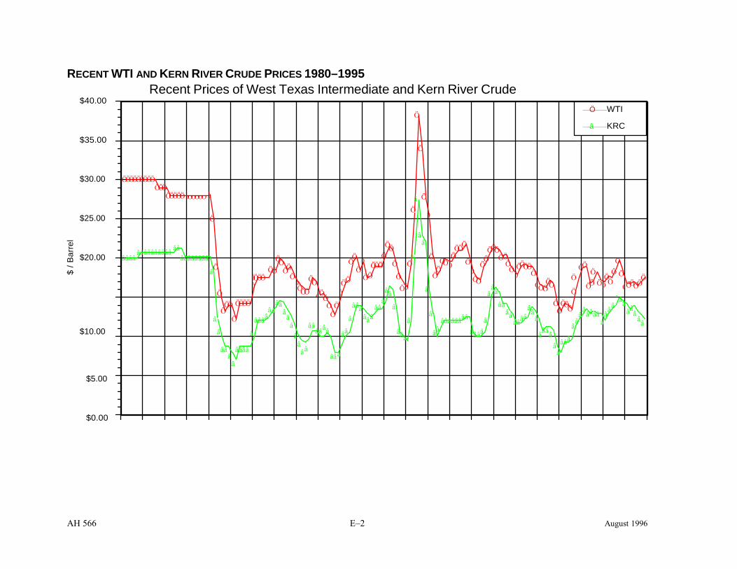
Ö Ö WTI

â KRC

Ö

Ö â Ö

Ö

Ö

ÖÖÖÖÖÖ

ââ

âÖ

Ö

Ö ÖÖÖÖ Ö

Ö ÖÖ ÖÖÖ Ö Ö

Ö Ö

ÖÖ

Ö

Ö ÖÖÖ ÖÖ

Ö

Ö

ââ Ö

Ö

Ö â

ÖÖ Ö

Ö Ö Ö Ö

Ö ÖÖ

â â

Ö Ö

â

ÖÖÖÖ Ö Ö

Ö

ÖÖ ÖÖ

Ö Ö

Ö

Ö Ö

ÖÖ Ö

Ö

Ö Ö Ö

Ö Ö Ö

â

â â âââ

Ö â

ÖÖ Ö

Ö

RECENT WTI AND KERN RIVER CRUDE PRICES 1980–1995 Recent Prices of West Texas Intermediate and Kern River Crude

$40.00

$35.00

$30.00

$25.00

ÖÖÖÖÖÖÖÖÖ ÖÖÖ

ÖÖÖÖÖ

Ö

$20.00 ââââ ââââââââ ââ

ââââââââ ÖÖ

â â ÖÖ ÖÖ

Ö Ö â Ö Ö ÖÖÖ

Ö ÖÖ

$10.00

ÖÖ ÖÖÖÖ Ö

â Ö

â â

â ââââ

Ö ÖÖ Ö

ââ â â

â â

â â

Ö Ö Ö

Ö ââ

ââââ

ââââ

ââ

â ââ

âââ

â

â âââ

â ââââââââ

ââ

â ââââ

ââ â

ââ â ââââ

â

ââââ

Ö ÖÖ Ö

â

âââââ ââ

â â

Ö

Ö

â ââ

âââ

$5.00

ââ ââââ â

â ââ

âââ

$0.00

$ / B

arre

l

â â

AH 566 E–22 August 1996

AH 566 F – 1 August 1996

APPENDIX F: PETROLEUM ENGINEERING AND PRODUCTION SYMBOLS, ABBREVIATIONS AND

DEFINITIONS

There is a large array of symbols and abbreviations in use in the petroleum industry. The symbols are used mainly in the field of reservoir engineering , and have been standardized by the Society of Petroleum Engineers. The abbreviations are use mainly by oil scouts and production personnel; They are commonly found in well scout reports and in well histories and production reports.

The symbols and abbreviation are variously used for gas only, for oil only, or for both oil and gas. They are consolidated here in this appendix for ready reference in reading the chapters on oil and gas reserve estimation.

Abbreviations 43.56 Thousands of square feet in one acre–foot

A area, usually in acres

A/ft acre–foot or acre–feet; an acre–foot is the bulk volume of one acre area with a thickness of one–foot

bn bean; a fixed or adjustable flow orifice; bean sizes are usually notes in diameters which are multiples of 1/64 of an inch

BHP Bottom–hole pressure, in psi

CP Casing pressure; this pressure may be read on a gauge attached to the casing head of the well

FP flow pressure or flowing pressure; This is the pressure in the tubing while the well is producing. It may be measured by gauges placed either at the surface or near the bottom of the well. The flowing pressure is a back pressure, which decreases with the use of large beans and higher flow rates.

MCF 100 cubic feet of gas , usually stated in terms of standard conditions of pressure and temperature (generally 14.73 psia and 60ºF). The MCF is the basic unit of volume for gas measurement.

pf, perfs perforations in the casing or liner of a well, for purposes of production or for testing for water shut–off. Perforated intervals are given in terms of the well depth at the top and bottom of the interval.

AH 566 F–2 August 1996

SI shut in; commonly a gas well is flow–tested in the process of completing it, and the well is then “shut in,” i.e., all flow valves are closed until such time as the well is hooked up to the sales line. Wells may also be shut in temporarily for repair purposes, at times when the demand for gas is low, or for pressure studies.

TP tubing pressure; pressure measured at the surface within the tubing, which is the pipe, usually 1 1/2 to 2 1/2 inches in internal diameter, within the casing through which the gas flows from the reservoirs and to the wellhead.

Symbols

B formation volume factor; the volume at reservoir conditions divided by the volume at standard conditions

Bg gas formation volume factor

Bo oil formation volume factor

D depth

ER reservoir recovery efficiency, or “recovery factor”; the percent of total oil or gas in place which may be economically recovered. The recovery factor may be affected by sand permeability, reservoir water drive, gas field line pressure, or other factors.

G total initial gas in place in reservoir

Gp cumulative gas produced

∆Gp gas produce during an interval

h thickness (in general or of a particular bed)

ln natural logarithm, base e

M molecular weight

n total moles

N initial oil in place in reservoir

Np Cumulative oil production

∆Np oil produced during an interval

p pressure (usually in pounds per square inch or psi

AH 566 F – 3 August 1996

pa atmospheric pressure

pcf casing pressure, flowing

pcs casing pressure, static

pi initial pressure

pR pressure at reservoir conditions; for practical purposes this is the pressure at the midpoint of the producing sand. If a pressure is not available, it may be approximated for a virgin reservoir by multiplying the depth in feet by 0.433 in areas where hydrostatic conditions prevail. This method is not usable in areas such as the Colusa Basin, where pressures exceed hydrostatic.

Psc pressure, standard conditions; usually 14.73 psia in California

pws static bottom hole pressure; this is equal to pR if the shut–in bottomhole pressure is given time to stabilize.

q production rate or flow rate

qg gas production rate

qo oil production rate

R producing gas/oil ratio

R universal gas constant (per mole)

Rp cumulative gas/oil ratio

Rs solution gas/oil ratio (gas solubility in oil)

Rsi initial solution gas/oil ratio

S saturation

Sw water saturation; even in commercial oil or gas sand part of the pore space is filled with water. Water saturation is expressed as a percent of the pore space itself. This reduces the pore space which is available for hydrocarbons; if, for example, a sand has 30% porosity and 40% of the pore space is saturated with water, this means that .40x.30 or 12% of the total volume of the sand is filled with water, leaving a porosity for hydrocarbons of 30-12, or 18%. Water saturation is expressed as a decimal fraction in the volumetric formula.

AH 566 F–4 August 1996

t time

T temperature; this may be expressed either in degrees Fahrenheit (°F) or in degrees Rankin absolute (°R); °R is equal to °F plus 460. Absolute temperature, i.e. degrees Rankin, must always be employed in gas calculations.

TR reservoir temperature. This may often be obtained from temperature surveys run in the well. If it is not available, an estimate may be made by adding to the mean surface temperature, one and one–half degrees for each 100 feet of depth. For example, the temperature at 5,000 feet may be estimated at 60 plus 75, or 135 °F (595 °R).

Tsc temperature at standard conditions. For gas evaluation this is 60 °F (520 °R).

z gas deviation factor (or compressibility factor); this must be calculated for each BHP or PR used. Calculations of the z–factor is discussed in chapter V. Use is sometimes made of Y, which is the reciprocal of z.

Greek Letters

γ gamma; specific gravity

∆ delta; difference

µ mu; viscosity

φ phi; porosity; porosity is expressed in the volumetric formula as a decimal fraction, i.e., 15% becomes 0.15.

AH 566 F – 5 August 1996

Bibliography Craft, B.C. and Hawkins, M.F., 1959, Applied Petroleum Reservoir Engineering: Prentice–Hall, Inc., Englewood Cliffs, N.J.

Mayer, E.H, 1964, “Committee Proposes Revised Symbol List to SPE Membership,” Journal of Petroleum Technology, Soc. of Petroleum Engineers, Dallas, Texas, June, pp. 649–656

APPENDIX G: PRESENT WORTH FACTORS- MID-YEAR

Year 8% 8.50% 9% 9.50% 10% 10.50% 1 0.96225 0.96003 0.95783 0.95564 0.95346 0.95130 2 0.89097 0.88482 0.87874 0.87273 0.86678 0.86091 3 0.82497 0.81550 0.80618 0.79701 0.78799 0.77910 4 0.76387 0.75162 0.73962 0.72786 0.71635 0.70507 5 0.70728 0.69273 0.67855 0.66472 0.65123 0.63807 6 0.65489 0.63846 0.62252 0.60705 0.59203 0.57744 7 0.60638 0.58845 0.57112 0.55438 0.53820 0.52257 8 0.56146 0.54235 0.52396 0.50628 0.48928 0.47291 9 0.51987 0.49986 0.48070 0.46236 0.44480 0.42798

10 0.48136 0.46070 0.44101 0.42225 0.40436 0.38731 11 0.44571 0.42461 0.40460 0.38561 0.36760 0.35051 12 0.41269 0.39134 0.37119 0.35216 0.33418 0.31720 13 0.38212 0.36069 0.34054 0.32161 0.30380 0.28706 14 0.35382 0.33243 0.31242 0.29370 0.27618 0.25978 15 0.32761 0.30639 0.28663 0.26822 0.25108 0.23510 16 0.30334 0.28238 0.26296 0.24495 0.22825 0.21276 17 0.28087 0.26026 0.24125 0.22370 0.20750 0.19254 18 0.26007 0.23987 0.22133 0.20429 0.18864 0.17424 19 0.24080 0.22108 0.20305 0.18657 0.17149 0.15769 20 0.22297 0.20376 0.18629 0.17038 0.15590 0.14270 21 0.20645 0.18780 0.17091 0.15560 0.14173 0.12914 22 0.19116 0.17309 0.15679 0.14210 0.12884 0.11687 23 0.17700 0.15953 0.14385 0.12977 0.11713 0.10577 24 0.16389 0.14703 0.13197 0.11851 0.10648 0.09572 25 0.15175 0.13551 0.12107 0.10823 0.09680 0.08662 26 0.14051 0.12489 0.11108 0.09884 0.08800 0.07839 27 0.13010 0.11511 0.10191 0.09027 0.08000 0.07094 28 0.12046 0.10609 0.09349 0.08244 0.07273 0.06420 29 0.11154 0.09778 0.08577 0.07528 0.06612 0.05810 30 0.10328 0.09012 0.07869 0.06875 0.06011 0.05258 31 0.09563 0.08306 0.07219 0.06279 0.05464 0.04758 32 0.08854 0.07655 0.06623 0.05734 0.04967 0.04306 33 0.08198 0.07056 0.06076 0.05237 0.04516 0.03897 34 0.07591 0.06503 0.05575 0.04782 0.04105 0.03527 35 0.07029 0.05993 0.05114 0.04367 0.03732 0.03192 36 0.06508 0.05524 0.04692 0.03988 0.03393 0.02888 37 0.06026 0.05091 0.04305 0.03642 0.03084 0.02614 38 0.05580 0.04692 0.03949 0.03326 0.02804 0.02365 39 0.05166 0.04325 0.03623 0.03038 0.02549 0.02141 40 0.04784 0.03986 0.03324 0.02774 0.02317 0.01937

AH 566 G-1 August 1996

Mid-Year Discount Factors

Year 11% 11.50% 12% 12.50% 13% 13.50% 1 0.94916 0.94703 0.94491 0.94281 0.94072 0.93865 2 0.85510 0.84935 0.84367 0.83805 0.83250 0.82700 3 0.77036 0.76175 0.75328 0.74494 0.73672 0.72864 4 0.69402 0.68318 0.67257 0.66216 0.65197 0.64197 5 0.62524 0.61272 0.60051 0.58859 0.57696 0.56561 6 0.56328 0.54953 0.53617 0.52319 0.51059 0.49834 7 0.50746 0.49285 0.47872 0.46506 0.45185 0.43906 8 0.45717 0.44202 0.42743 0.41339 0.39986 0.38684 9 0.41186 0.39643 0.38163 0.36745 0.35386 0.34083

10 0.37105 0.35554 0.34074 0.32663 0.31315 0.30029 11 0.33428 0.31887 0.30424 0.29033 0.27713 0.26457 12 0.30115 0.28598 0.27164 0.25808 0.24524 0.23310 13 0.27131 0.25649 0.24254 0.22940 0.21703 0.20538 14 0.24442 0.23003 0.21655 0.20391 0.19206 0.18095 15 0.22020 0.20631 0.19335 0.18125 0.16997 0.15943 16 0.19838 0.18503 0.17263 0.16111 0.15041 0.14046 17 0.17872 0.16595 0.15414 0.14321 0.13311 0.12376 18 0.16101 0.14883 0.13762 0.12730 0.11780 0.10904 19 0.14505 0.13348 0.12288 0.11316 0.10424 0.09607 20 0.13068 0.11971 0.10971 0.10058 0.09225 0.08464 21 0.11773 0.10737 0.09796 0.08941 0.08164 0.07457 22 0.10606 0.09629 0.08746 0.07947 0.07225 0.06570 23 0.09555 0.08636 0.07809 0.07064 0.06393 0.05789 24 0.08608 0.07745 0.06972 0.06279 0.05658 0.05100 25 0.07755 0.06946 0.06225 0.05582 0.05007 0.04494 26 0.06987 0.06230 0.05558 0.04961 0.04431 0.03959 27 0.06294 0.05587 0.04963 0.04410 0.03921 0.03488 28 0.05670 0.05011 0.04431 0.03920 0.03470 0.03073 29 0.05109 0.04494 0.03956 0.03485 0.03071 0.02708 30 0.04602 0.04031 0.03532 0.03097 0.02718 0.02386 31 0.04146 0.03615 0.03154 0.02753 0.02405 0.02102 32 0.03735 0.03242 0.02816 0.02447 0.02128 0.01852 33 0.03365 0.02908 0.02514 0.02175 0.01883 0.01632 34 0.03032 0.02608 0.02245 0.01934 0.01667 0.01438 35 0.02731 0.02339 0.02004 0.01719 0.01475 0.01267 36 0.02461 0.02098 0.01790 0.01528 0.01305 0.01116 37 0.02217 0.01881 0.01598 0.01358 0.01155 0.00983 38 0.01997 0.01687 0.01427 0.01207 0.01022 0.00866 39 0.01799 0.01513 0.01274 0.01073 0.00905 0.00763 40 0.01621 0.01357 0.01137 0.00954 0.00801 0.00672

AH 566 G-2 August 1996

Mid-Year Discount Factors

Year 14% 14.50% 15% 15.50% 16% 16.50% 1 0.93659 0.93454 0.93250 0.93048 0.92848 0.92648 2 0.82157 0.81619 0.81087 0.80561 0.80041 0.79526 3 0.72067 0.71283 0.70511 0.69750 0.69001 0.68263 4 0.63217 0.62256 0.61314 0.60390 0.59484 0.58595 5 0.55453 0.54372 0.53316 0.52285 0.51279 0.50296 6 0.48643 0.47486 0.46362 0.45269 0.44206 0.43173 7 0.42670 0.41473 0.40315 0.39194 0.38109 0.37058 8 0.37429 0.36221 0.35056 0.33934 0.32852 0.31809 9 0.32833 0.31634 0.30484 0.29380 0.28321 0.27304

10 0.28801 0.27628 0.26508 0.25437 0.24415 0.23437 11 0.25264 0.24129 0.23050 0.22024 0.21047 0.20118 12 0.22161 0.21074 0.20044 0.19068 0.18144 0.17268 13 0.19440 0.18405 0.17429 0.16509 0.15641 0.14823 14 0.17052 0.16074 0.15156 0.14294 0.13484 0.12723 15 0.14958 0.14038 0.13179 0.12375 0.11624 0.10921 16 0.13121 0.12261 0.11460 0.10715 0.10021 0.09375 17 0.11510 0.10708 0.09965 0.09277 0.08639 0.08047 18 0.10096 0.09352 0.08665 0.08032 0.07447 0.06907 19 0.08856 0.08168 0.07535 0.06954 0.06420 0.05929 20 0.07769 0.07133 0.06552 0.06021 0.05534 0.05089 21 0.06815 0.06230 0.05698 0.05213 0.04771 0.04368 22 0.05978 0.05441 0.04954 0.04513 0.04113 0.03750 23 0.05244 0.04752 0.04308 0.03908 0.03546 0.03219 24 0.04600 0.04150 0.03746 0.03383 0.03057 0.02763 25 0.04035 0.03625 0.03258 0.02929 0.02635 0.02371 26 0.03539 0.03166 0.02833 0.02536 0.02272 0.02036 27 0.03105 0.02765 0.02463 0.02196 0.01958 0.01747 28 0.02723 0.02415 0.02142 0.01901 0.01688 0.01500 29 0.02389 0.02109 0.01863 0.01646 0.01455 0.01287 30 0.02096 0.01842 0.01620 0.01425 0.01255 0.01105 31 0.01838 0.01609 0.01408 0.01234 0.01082 0.00949 32 0.01612 0.01405 0.01225 0.01068 0.00932 0.00814 33 0.01414 0.01227 0.01065 0.00925 0.00804 0.00699 34 0.01241 0.01072 0.00926 0.00801 0.00693 0.00600 35 0.01088 0.00936 0.00805 0.00693 0.00597 0.00515 36 0.00955 0.00817 0.00700 0.00600 0.00515 0.00442 37 0.00837 0.00714 0.00609 0.00520 0.00444 0.00379 38 0.00735 0.00623 0.00529 0.00450 0.00383 0.00326 39 0.00644 0.00544 0.00460 0.00390 0.00330 0.00280 40 0.00565 0.00476 0.00400 0.00337 0.00284 0.00240

AH 566 G-3 August 1996

Mid-Year Discount Factors

Year 17% 17.50% 18% 18.50% 19% 19.50% 1 0.92450 0.92253 0.92057 0.91863 0.91670 0.91478 2 0.79017 0.78513 0.78015 0.77522 0.77033 0.76551 3 0.67536 0.66820 0.66114 0.65419 0.64734 0.64059 4 0.57723 0.56868 0.56029 0.55206 0.54398 0.53606 5 0.49336 0.48398 0.47482 0.46587 0.45713 0.44858 6 0.42167 0.41190 0.40239 0.39314 0.38414 0.37538 7 0.36041 0.35055 0.34101 0.33177 0.32281 0.31413 8 0.30804 0.29834 0.28899 0.27997 0.27127 0.26287 9 0.26328 0.25391 0.24491 0.23626 0.22796 0.21997

10 0.22503 0.21609 0.20755 0.19938 0.19156 0.18408 11 0.19233 0.18391 0.17589 0.16825 0.16097 0.15404 12 0.16439 0.15652 0.14906 0.14198 0.13527 0.12890 13 0.14050 0.13321 0.12632 0.11982 0.11367 0.10787 14 0.12009 0.11337 0.10705 0.10111 0.09552 0.09027 15 0.10264 0.09648 0.09072 0.08533 0.08027 0.07554 16 0.08772 0.08211 0.07688 0.07201 0.06746 0.06321 17 0.07498 0.06988 0.06515 0.06076 0.05669 0.05290 18 0.06408 0.05948 0.05522 0.05128 0.04764 0.04427 19 0.05477 0.05062 0.04679 0.04327 0.04003 0.03704 20 0.04681 0.04308 0.03966 0.03652 0.03364 0.03100 21 0.04001 0.03666 0.03361 0.03082 0.02827 0.02594 22 0.03420 0.03120 0.02848 0.02600 0.02375 0.02171 23 0.02923 0.02656 0.02414 0.02195 0.01996 0.01816 24 0.02498 0.02260 0.02045 0.01852 0.01677 0.01520 25 0.02135 0.01923 0.01733 0.01563 0.01410 0.01272 26 0.01825 0.01637 0.01469 0.01319 0.01185 0.01064 27 0.01560 0.01393 0.01245 0.01113 0.00995 0.00891 28 0.01333 0.01186 0.01055 0.00939 0.00836 0.00745 29 0.01139 0.01009 0.00894 0.00793 0.00703 0.00624 30 0.00974 0.00859 0.00758 0.00669 0.00591 0.00522 31 0.00832 0.00731 0.00642 0.00564 0.00496 0.00437 32 0.00711 0.00622 0.00544 0.00476 0.00417 0.00366 33 0.00608 0.00529 0.00461 0.00402 0.00351 0.00306 34 0.00520 0.00451 0.00391 0.00339 0.00295 0.00256 35 0.00444 0.00383 0.00331 0.00286 0.00248 0.00214 36 0.00380 0.00326 0.00281 0.00242 0.00208 0.00179 37 0.00325 0.00278 0.00238 0.00204 0.00175 0.00150 38 0.00277 0.00236 0.00202 0.00172 0.00147 0.00126 39 0.00237 0.00201 0.00171 0.00145 0.00123 0.00105 40 0.00203 0.00171 0.00145 0.00122 0.00104 0.00088

AH 566 G-4 August 1996

Mid-Year Discount Factors

Year 20% 20.50% 21% 21.50% 22% 22.50% 1 0.91287 0.91098 0.90909 0.90722 0.90536 0.90351 2 0.76073 0.75600 0.75131 0.74668 0.74210 0.73756 3 0.63394 0.62738 0.62092 0.61455 0.60828 0.60209 4 0.52828 0.52065 0.51316 0.50580 0.49859 0.49150 5 0.44023 0.43207 0.42410 0.41630 0.40868 0.40122 6 0.36686 0.35857 0.35049 0.34263 0.33498 0.32753 7 0.30572 0.29757 0.28966 0.28200 0.27458 0.26737 8 0.25477 0.24694 0.23939 0.23210 0.22506 0.21826 9 0.21230 0.20493 0.19784 0.19103 0.18448 0.17817

10 0.17692 0.17007 0.16351 0.15723 0.15121 0.14545 11 0.14743 0.14114 0.13513 0.12940 0.12394 0.11873 12 0.12286 0.11712 0.11168 0.10651 0.10159 0.09692 13 0.10238 0.09720 0.09230 0.08766 0.08327 0.07912 14 0.08532 0.08066 0.07628 0.07215 0.06826 0.06459 15 0.07110 0.06694 0.06304 0.05938 0.05595 0.05273 16 0.05925 0.05555 0.05210 0.04887 0.04586 0.04304 17 0.04938 0.04610 0.04306 0.04022 0.03759 0.03514 18 0.04115 0.03826 0.03558 0.03311 0.03081 0.02868 19 0.03429 0.03175 0.02941 0.02725 0.02525 0.02341 20 0.02857 0.02635 0.02430 0.02243 0.02070 0.01911 21 0.02381 0.02187 0.02009 0.01846 0.01697 0.01560 22 0.01984 0.01815 0.01660 0.01519 0.01391 0.01274 23 0.01654 0.01506 0.01372 0.01250 0.01140 0.01040 24 0.01378 0.01250 0.01134 0.01029 0.00934 0.00849 25 0.01148 0.01037 0.00937 0.00847 0.00766 0.00693 26 0.00957 0.00861 0.00774 0.00697 0.00628 0.00566 27 0.00797 0.00714 0.00640 0.00574 0.00515 0.00462 28 0.00665 0.00593 0.00529 0.00472 0.00422 0.00377 29 0.00554 0.00492 0.00437 0.00389 0.00346 0.00308 30 0.00461 0.00408 0.00361 0.00320 0.00283 0.00251 31 0.00385 0.00339 0.00299 0.00263 0.00232 0.00205 32 0.00320 0.00281 0.00247 0.00217 0.00190 0.00167 33 0.00267 0.00233 0.00204 0.00178 0.00156 0.00137 34 0.00223 0.00194 0.00169 0.00147 0.00128 0.00112 35 0.00185 0.00161 0.00139 0.00121 0.00105 0.00091 36 0.00155 0.00133 0.00115 0.00099 0.00086 0.00074 37 0.00129 0.00111 0.00095 0.00082 0.00070 0.00061 38 0.00107 0.00092 0.00079 0.00067 0.00058 0.00050 39 0.00089 0.00076 0.00065 0.00055 0.00047 0.00040 40 0.00075 0.00063 0.00054 0.00046 0.00039 0.00033

AH 566 G-5 August 1996

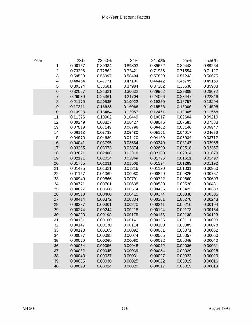
Mid-Year Discount Factors

Year 23% 23.50% 24% 24.50% 25% 25.50% 1 0.90167 0.89984 0.89803 0.89622 0.89443 0.89264 2 0.73306 0.72862 0.72421 0.71986 0.71554 0.71127 3 0.59599 0.58997 0.58404 0.57820 0.57243 0.56675 4 0.48454 0.47771 0.47100 0.46442 0.45795 0.45159 5 0.39394 0.38681 0.37984 0.37302 0.36636 0.35983 6 0.32027 0.31321 0.30632 0.29962 0.29309 0.28672 7 0.26039 0.25361 0.24704 0.24066 0.23447 0.22846 8 0.21170 0.20535 0.19922 0.19330 0.18757 0.18204 9 0.17211 0.16628 0.16066 0.15526 0.15006 0.14505

10 0.13993 0.13464 0.12957 0.12471 0.12005 0.11558 11 0.11376 0.10902 0.10449 0.10017 0.09604 0.09210 12 0.09249 0.08827 0.08427 0.08045 0.07683 0.07338 13 0.07519 0.07148 0.06796 0.06462 0.06146 0.05847 14 0.06113 0.05788 0.05480 0.05191 0.04917 0.04659 15 0.04970 0.04686 0.04420 0.04169 0.03934 0.03712 16 0.04041 0.03795 0.03564 0.03349 0.03147 0.02958 17 0.03285 0.03073 0.02874 0.02690 0.02518 0.02357 18 0.02671 0.02488 0.02318 0.02160 0.02014 0.01878 19 0.02171 0.02014 0.01869 0.01735 0.01611 0.01497 20 0.01765 0.01631 0.01508 0.01394 0.01289 0.01192 21 0.01435 0.01321 0.01216 0.01120 0.01031 0.00950 22 0.01167 0.01069 0.00980 0.00899 0.00825 0.00757 23 0.00949 0.00866 0.00791 0.00722 0.00660 0.00603 24 0.00771 0.00701 0.00638 0.00580 0.00528 0.00481 25 0.00627 0.00568 0.00514 0.00466 0.00422 0.00383 26 0.00510 0.00460 0.00415 0.00374 0.00338 0.00305 27 0.00414 0.00372 0.00334 0.00301 0.00270 0.00243 28 0.00337 0.00301 0.00270 0.00241 0.00216 0.00194 29 0.00274 0.00244 0.00218 0.00194 0.00173 0.00154 30 0.00223 0.00198 0.00175 0.00156 0.00138 0.00123 31 0.00181 0.00160 0.00141 0.00125 0.00111 0.00098 32 0.00147 0.00130 0.00114 0.00100 0.00089 0.00078 33 0.00120 0.00105 0.00092 0.00081 0.00071 0.00062 34 0.00097 0.00085 0.00074 0.00065 0.00057 0.00050 35 0.00079 0.00069 0.00060 0.00052 0.00045 0.00040 36 0.00064 0.00056 0.00048 0.00042 0.00036 0.00031 37 0.00052 0.00045 0.00039 0.00034 0.00029 0.00025 38 0.00043 0.00037 0.00031 0.00027 0.00023 0.00020 39 0.00035 0.00030 0.00025 0.00022 0.00019 0.00016 40 0.00028 0.00024 0.00020 0.00017 0.00015 0.00013

AH 566 G-6 August 1996

Mid-Year Discount Factors

Year 26% 26.50% 27% 27.50% 28% 28.50% 1 0.89087 0.88911 0.88736 0.88561 0.88388 0.88216 2 0.70704 0.70285 0.69871 0.69460 0.69053 0.68651 3 0.56114 0.55561 0.55016 0.54478 0.53948 0.53425 4 0.44535 0.43922 0.43320 0.42728 0.42147 0.41576 5 0.35345 0.34721 0.34110 0.33512 0.32927 0.32355 6 0.28052 0.27447 0.26858 0.26284 0.25724 0.25179 7 0.22263 0.21698 0.21148 0.20615 0.20097 0.19594 8 0.17669 0.17152 0.16652 0.16169 0.15701 0.15248 9 0.14023 0.13559 0.13112 0.12681 0.12266 0.11867

10 0.11130 0.10719 0.10324 0.09946 0.09583 0.09235 11 0.08833 0.08473 0.08129 0.07801 0.07487 0.07186 12 0.07010 0.06698 0.06401 0.06118 0.05849 0.05593 13 0.05564 0.05295 0.05040 0.04799 0.04570 0.04352 14 0.04416 0.04186 0.03969 0.03764 0.03570 0.03387 15 0.03505 0.03309 0.03125 0.02952 0.02789 0.02636 16 0.02781 0.02616 0.02461 0.02315 0.02179 0.02051 17 0.02207 0.02068 0.01937 0.01816 0.01702 0.01596 18 0.01752 0.01635 0.01526 0.01424 0.01330 0.01242 19 0.01390 0.01292 0.01201 0.01117 0.01039 0.00967 20 0.01104 0.01021 0.00946 0.00876 0.00812 0.00752 21 0.00876 0.00808 0.00745 0.00687 0.00634 0.00585 22 0.00695 0.00638 0.00586 0.00539 0.00495 0.00456 23 0.00552 0.00505 0.00462 0.00423 0.00387 0.00355 24 0.00438 0.00399 0.00364 0.00332 0.00302 0.00276 25 0.00347 0.00315 0.00286 0.00260 0.00236 0.00215 26 0.00276 0.00249 0.00225 0.00204 0.00185 0.00167 27 0.00219 0.00197 0.00178 0.00160 0.00144 0.00130 28 0.00174 0.00156 0.00140 0.00125 0.00113 0.00101 29 0.00138 0.00123 0.00110 0.00098 0.00088 0.00079 30 0.00109 0.00097 0.00087 0.00077 0.00069 0.00061 31 0.00087 0.00077 0.00068 0.00061 0.00054 0.00048 32 0.00069 0.00061 0.00054 0.00047 0.00042 0.00037 33 0.00055 0.00048 0.00042 0.00037 0.00033 0.00029 34 0.00043 0.00038 0.00033 0.00029 0.00026 0.00022 35 0.00034 0.00030 0.00026 0.00023 0.00020 0.00017 36 0.00027 0.00024 0.00021 0.00018 0.00016 0.00014 37 0.00022 0.00019 0.00016 0.00014 0.00012 0.00011 38 0.00017 0.00015 0.00013 0.00011 0.00010 0.00008 39 0.00014 0.00012 0.00010 0.00009 0.00007 0.00006 40 0.00011 0.00009 0.00008 0.00007 0.00006 0.00005

AH 566 G-7 August 1996

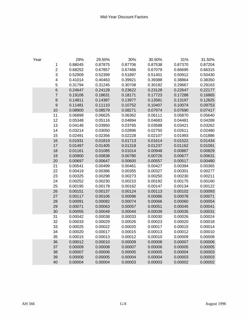
Mid-Year Discount Factors

Year 29% 29.50% 30% 30.50% 31% 31.50% 1 0.88045 0.87875 0.87706 0.87538 0.87370 0.87204 2 0.68252 0.67857 0.67466 0.67079 0.66695 0.66315 3 0.52909 0.52399 0.51897 0.51401 0.50912 0.50430 4 0.41014 0.40463 0.39921 0.39388 0.38864 0.38350 5 0.31794 0.31245 0.30708 0.30182 0.29667 0.29163 6 0.24647 0.24128 0.23622 0.23128 0.22647 0.22177 7 0.19106 0.18631 0.18171 0.17723 0.17288 0.16865 8 0.14811 0.14387 0.13977 0.13581 0.13197 0.12825 9 0.11481 0.11110 0.10752 0.10407 0.10074 0.09753

10 0.08900 0.08579 0.08271 0.07974 0.07690 0.07417 11 0.06899 0.06625 0.06362 0.06111 0.05870 0.05640 12 0.05348 0.05116 0.04894 0.04683 0.04481 0.04289 13 0.04146 0.03950 0.03765 0.03588 0.03421 0.03262 14 0.03214 0.03050 0.02896 0.02750 0.02611 0.02480 15 0.02491 0.02356 0.02228 0.02107 0.01993 0.01886 16 0.01931 0.01819 0.01713 0.01614 0.01522 0.01434 17 0.01497 0.01405 0.01318 0.01237 0.01162 0.01091 18 0.01161 0.01085 0.01014 0.00948 0.00887 0.00829 19 0.00900 0.00838 0.00780 0.00726 0.00677 0.00631 20 0.00697 0.00647 0.00600 0.00557 0.00517 0.00480 21 0.00541 0.00499 0.00461 0.00427 0.00394 0.00365 22 0.00419 0.00386 0.00355 0.00327 0.00301 0.00277 23 0.00325 0.00298 0.00273 0.00250 0.00230 0.00211 24 0.00252 0.00230 0.00210 0.00192 0.00175 0.00160 25 0.00195 0.00178 0.00162 0.00147 0.00134 0.00122 26 0.00151 0.00137 0.00124 0.00113 0.00102 0.00093 27 0.00117 0.00106 0.00096 0.00086 0.00078 0.00071 28 0.00091 0.00082 0.00074 0.00066 0.00060 0.00054 29 0.00071 0.00063 0.00057 0.00051 0.00045 0.00041 30 0.00055 0.00049 0.00044 0.00039 0.00035 0.00031 31 0.00042 0.00038 0.00033 0.00030 0.00026 0.00024 32 0.00033 0.00029 0.00026 0.00023 0.00020 0.00018 33 0.00025 0.00022 0.00020 0.00017 0.00015 0.00014 34 0.00020 0.00017 0.00015 0.00013 0.00012 0.00010 35 0.00015 0.00013 0.00012 0.00010 0.00009 0.00008 36 0.00012 0.00010 0.00009 0.00008 0.00007 0.00006 37 0.00009 0.00008 0.00007 0.00006 0.00005 0.00005 38 0.00007 0.00006 0.00005 0.00005 0.00004 0.00003 39 0.00006 0.00005 0.00004 0.00004 0.00003 0.00003 40 0.00004 0.00004 0.00003 0.00003 0.00002 0.00002

AH 566 G-8 August 1996

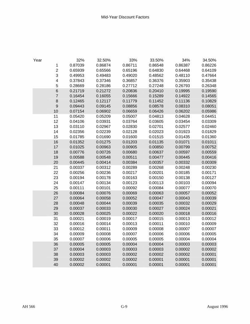
Mid-Year Discount Factors

Year 32% 32.50% 33% 33.50% 34% 34.50% 1 0.87039 0.86874 0.86711 0.86548 0.86387 0.86226 2 0.65939 0.65566 0.65196 0.64830 0.64468 0.64109 3 0.49953 0.49483 0.49020 0.48562 0.48110 0.47664 4 0.37843 0.37346 0.36857 0.36376 0.35903 0.35438 5 0.28669 0.28186 0.27712 0.27248 0.26793 0.26348 6 0.21719 0.21272 0.20836 0.20410 0.19995 0.19590 7 0.16454 0.16055 0.15666 0.15289 0.14922 0.14565 8 0.12465 0.12117 0.11779 0.11452 0.11136 0.10829 9 0.09443 0.09145 0.08856 0.08578 0.08310 0.08051

10 0.07154 0.06902 0.06659 0.06426 0.06202 0.05986 11 0.05420 0.05209 0.05007 0.04813 0.04628 0.04451 12 0.04106 0.03931 0.03764 0.03605 0.03454 0.03309 13 0.03110 0.02967 0.02830 0.02701 0.02577 0.02460 14 0.02356 0.02239 0.02128 0.02023 0.01923 0.01829 15 0.01785 0.01690 0.01600 0.01515 0.01435 0.01360 16 0.01352 0.01275 0.01203 0.01135 0.01071 0.01011 17 0.01025 0.00963 0.00905 0.00850 0.00799 0.00752 18 0.00776 0.00726 0.00680 0.00637 0.00597 0.00559 19 0.00588 0.00548 0.00511 0.00477 0.00445 0.00416 20 0.00445 0.00414 0.00384 0.00357 0.00332 0.00309 21 0.00337 0.00312 0.00289 0.00268 0.00248 0.00230 22 0.00256 0.00236 0.00217 0.00201 0.00185 0.00171 23 0.00194 0.00178 0.00163 0.00150 0.00138 0.00127 24 0.00147 0.00134 0.00123 0.00113 0.00103 0.00094 25 0.00111 0.00101 0.00092 0.00084 0.00077 0.00070 26 0.00084 0.00076 0.00069 0.00063 0.00057 0.00052 27 0.00064 0.00058 0.00052 0.00047 0.00043 0.00039 28 0.00048 0.00044 0.00039 0.00035 0.00032 0.00029 29 0.00037 0.00033 0.00030 0.00027 0.00024 0.00021 30 0.00028 0.00025 0.00022 0.00020 0.00018 0.00016 31 0.00021 0.00019 0.00017 0.00015 0.00013 0.00012 32 0.00016 0.00014 0.00013 0.00011 0.00010 0.00009 33 0.00012 0.00011 0.00009 0.00008 0.00007 0.00007 34 0.00009 0.00008 0.00007 0.00006 0.00006 0.00005 35 0.00007 0.00006 0.00005 0.00005 0.00004 0.00004 36 0.00005 0.00005 0.00004 0.00004 0.00003 0.00003 37 0.00004 0.00003 0.00003 0.00003 0.00002 0.00002 38 0.00003 0.00003 0.00002 0.00002 0.00002 0.00001 39 0.00002 0.00002 0.00002 0.00001 0.00001 0.00001 40 0.00002 0.00001 0.00001 0.00001 0.00001 0.00001

AH 566 G-9 August 1996

Mid-Year Discount Factors

Year 35% 35.50% 36% 36.50% 37% 37.50% 1 0.86066 0.85907 0.85749 0.85592 0.85436 0.85280 2 0.63753 0.63400 0.63051 0.62705 0.62362 0.62022 3 0.47224 0.46790 0.46361 0.45938 0.45520 0.45107 4 0.34981 0.34531 0.34089 0.33654 0.33226 0.32805 5 0.25912 0.25484 0.25065 0.24655 0.24253 0.23858 6 0.19194 0.18808 0.18430 0.18062 0.17703 0.17351 7 0.14218 0.13880 0.13552 0.13232 0.12922 0.12619 8 0.10532 0.10244 0.09965 0.09694 0.09432 0.09178 9 0.07801 0.07560 0.07327 0.07102 0.06885 0.06675

10 0.05779 0.05579 0.05387 0.05203 0.05025 0.04854 11 0.04281 0.04118 0.03961 0.03812 0.03668 0.03530 12 0.03171 0.03039 0.02913 0.02792 0.02677 0.02568 13 0.02349 0.02243 0.02142 0.02046 0.01954 0.01867 14 0.01740 0.01655 0.01575 0.01499 0.01427 0.01358 15 0.01289 0.01221 0.01158 0.01098 0.01041 0.00988 16 0.00955 0.00901 0.00851 0.00804 0.00760 0.00718 17 0.00707 0.00665 0.00626 0.00589 0.00555 0.00522 18 0.00524 0.00491 0.00460 0.00432 0.00405 0.00380 19 0.00388 0.00362 0.00338 0.00316 0.00296 0.00276 20 0.00287 0.00267 0.00249 0.00232 0.00216 0.00201 21 0.00213 0.00197 0.00183 0.00170 0.00157 0.00146 22 0.00158 0.00146 0.00135 0.00124 0.00115 0.00106 23 0.00117 0.00107 0.00099 0.00091 0.00084 0.00077 24 0.00087 0.00079 0.00073 0.00067 0.00061 0.00056 25 0.00064 0.00059 0.00053 0.00049 0.00045 0.00041 26 0.00047 0.00043 0.00039 0.00036 0.00033 0.00030 27 0.00035 0.00032 0.00029 0.00026 0.00024 0.00022 28 0.00026 0.00024 0.00021 0.00019 0.00017 0.00016 29 0.00019 0.00017 0.00016 0.00014 0.00013 0.00011 30 0.00014 0.00013 0.00011 0.00010 0.00009 0.00008 31 0.00011 0.00009 0.00008 0.00008 0.00007 0.00006 32 0.00008 0.00007 0.00006 0.00006 0.00005 0.00004 33 0.00006 0.00005 0.00005 0.00004 0.00004 0.00003 34 0.00004 0.00004 0.00003 0.00003 0.00003 0.00002 35 0.00003 0.00003 0.00002 0.00002 0.00002 0.00002 36 0.00002 0.00002 0.00002 0.00002 0.00001 0.00001 37 0.00002 0.00002 0.00001 0.00001 0.00001 0.00001 38 0.00001 0.00001 0.00001 0.00001 0.00001 0.00001 39 0.00001 0.00001 0.00001 0.00001 0.00001 0.00000 40 0.00001 0.00001 0.00001 0.00000 0.00000 0.00000

AH 566 G-10 August 1996

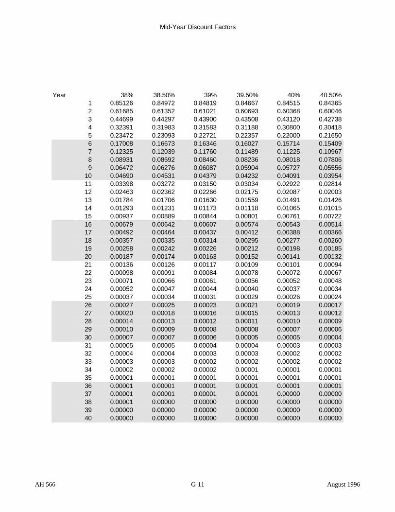
Mid-Year Discount Factors

Year 38% 38.50% 39% 39.50% 40% 40.50% 1 0.85126 0.84972 0.84819 0.84667 0.84515 0.84365 2 0.61685 0.61352 0.61021 0.60693 0.60368 0.60046 3 0.44699 0.44297 0.43900 0.43508 0.43120 0.42738 4 0.32391 0.31983 0.31583 0.31188 0.30800 0.30418 5 0.23472 0.23093 0.22721 0.22357 0.22000 0.21650 6 0.17008 0.16673 0.16346 0.16027 0.15714 0.15409 7 0.12325 0.12039 0.11760 0.11489 0.11225 0.10967 8 0.08931 0.08692 0.08460 0.08236 0.08018 0.07806 9 0.06472 0.06276 0.06087 0.05904 0.05727 0.05556

10 0.04690 0.04531 0.04379 0.04232 0.04091 0.03954 11 0.03398 0.03272 0.03150 0.03034 0.02922 0.02814 12 0.02463 0.02362 0.02266 0.02175 0.02087 0.02003 13 0.01784 0.01706 0.01630 0.01559 0.01491 0.01426 14 0.01293 0.01231 0.01173 0.01118 0.01065 0.01015 15 0.00937 0.00889 0.00844 0.00801 0.00761 0.00722 16 0.00679 0.00642 0.00607 0.00574 0.00543 0.00514 17 0.00492 0.00464 0.00437 0.00412 0.00388 0.00366 18 0.00357 0.00335 0.00314 0.00295 0.00277 0.00260 19 0.00258 0.00242 0.00226 0.00212 0.00198 0.00185 20 0.00187 0.00174 0.00163 0.00152 0.00141 0.00132 21 0.00136 0.00126 0.00117 0.00109 0.00101 0.00094 22 0.00098 0.00091 0.00084 0.00078 0.00072 0.00067 23 0.00071 0.00066 0.00061 0.00056 0.00052 0.00048 24 0.00052 0.00047 0.00044 0.00040 0.00037 0.00034 25 0.00037 0.00034 0.00031 0.00029 0.00026 0.00024 26 0.00027 0.00025 0.00023 0.00021 0.00019 0.00017 27 0.00020 0.00018 0.00016 0.00015 0.00013 0.00012 28 0.00014 0.00013 0.00012 0.00011 0.00010 0.00009 29 0.00010 0.00009 0.00008 0.00008 0.00007 0.00006 30 0.00007 0.00007 0.00006 0.00005 0.00005 0.00004 31 0.00005 0.00005 0.00004 0.00004 0.00003 0.00003 32 0.00004 0.00004 0.00003 0.00003 0.00002 0.00002 33 0.00003 0.00003 0.00002 0.00002 0.00002 0.00002 34 0.00002 0.00002 0.00002 0.00001 0.00001 0.00001 35 0.00001 0.00001 0.00001 0.00001 0.00001 0.00001 36 0.00001 0.00001 0.00001 0.00001 0.00001 0.00001 37 0.00001 0.00001 0.00001 0.00001 0.00000 0.00000 38 0.00001 0.00000 0.00000 0.00000 0.00000 0.00000 39 0.00000 0.00000 0.00000 0.00000 0.00000 0.00000 40 0.00000 0.00000 0.00000 0.00000 0.00000 0.00000

AH 566 G-11 August 1996

Mid-Year Discount Factors

Year 41% 41.50% 42% 42.50% 43% 43.50% 1 0.84215 0.84066 0.83918 0.83771 0.83624 0.83478 2 0.59727 0.59411 0.59097 0.58787 0.58478 0.58173 3 0.42360 0.41986 0.41618 0.41254 0.40894 0.40539 4 0.30042 0.29672 0.29308 0.28950 0.28597 0.28250 5 0.21307 0.20970 0.20640 0.20316 0.19998 0.19686 6 0.15111 0.14820 0.14535 0.14257 0.13985 0.13719 7 0.10717 0.10473 0.10236 0.10005 0.09779 0.09560 8 0.07601 0.07402 0.07208 0.07021 0.06839 0.06662 9 0.05391 0.05231 0.05076 0.04927 0.04782 0.04643

10 0.03823 0.03697 0.03575 0.03457 0.03344 0.03235 11 0.02711 0.02613 0.02518 0.02426 0.02339 0.02255 12 0.01923 0.01846 0.01773 0.01703 0.01635 0.01571 13 0.01364 0.01305 0.01249 0.01195 0.01144 0.01095 14 0.00967 0.00922 0.00879 0.00838 0.00800 0.00763 15 0.00686 0.00652 0.00619 0.00588 0.00559 0.00532 16 0.00487 0.00461 0.00436 0.00413 0.00391 0.00371 17 0.00345 0.00325 0.00307 0.00290 0.00273 0.00258 18 0.00245 0.00230 0.00216 0.00203 0.00191 0.00180 19 0.00174 0.00163 0.00152 0.00143 0.00134 0.00125 20 0.00123 0.00115 0.00107 0.00100 0.00094 0.00087 21 0.00087 0.00081 0.00076 0.00070 0.00065 0.00061 22 0.00062 0.00057 0.00053 0.00049 0.00046 0.00042 23 0.00044 0.00041 0.00037 0.00035 0.00032 0.00030 24 0.00031 0.00029 0.00026 0.00024 0.00022 0.00021 25 0.00022 0.00020 0.00019 0.00017 0.00016 0.00014 26 0.00016 0.00014 0.00013 0.00012 0.00011 0.00010 27 0.00011 0.00010 0.00009 0.00008 0.00008 0.00007 28 0.00008 0.00007 0.00006 0.00006 0.00005 0.00005 29 0.00006 0.00005 0.00005 0.00004 0.00004 0.00003 30 0.00004 0.00004 0.00003 0.00003 0.00003 0.00002 31 0.00003 0.00003 0.00002 0.00002 0.00002 0.00002 32 0.00002 0.00002 0.00002 0.00001 0.00001 0.00001 33 0.00001 0.00001 0.00001 0.00001 0.00001 0.00001 34 0.00001 0.00001 0.00001 0.00001 0.00001 0.00001 35 0.00001 0.00001 0.00001 0.00000 0.00000 0.00000 36 0.00001 0.00000 0.00000 0.00000 0.00000 0.00000 37 0.00000 0.00000 0.00000 0.00000 0.00000 0.00000 38 0.00000 0.00000 0.00000 0.00000 0.00000 0.00000 39 0.00000 0.00000 0.00000 0.00000 0.00000 0.00000 40 0.00000 0.00000 0.00000 0.00000 0.00000 0.00000

AH 566 G-12 August 1996

APPENDIX H: FORMS & WORKSHEETS

The SBE has approved four forms relating to petroleum properties, listed below. Copies of the forms are included in this appendix.

Form Number Title AH 566–D Oil and Dissolved Gas Production

Report AH 566–F Dry Gas Production, Equipment, New

Well, Redrill and Rework Report AH 566–J Oil, Gas, and Geothermal Personal

Property Statement AH 566–K Annual Oil and Gas Operating Expense

Data

The nature of the property will dictate which forms should be filed. Failure to file the proper form can result in a penalty of ten percent of the assessed value. See Sections 441 and 463 of the Revenue and Taxation Code.

Additional information may be required by the assessor to complete the appraisal. The request for this information must be made under a separate cover letter to avoid the confusion that failure to file the additional information could result in a penalty.

AH 566 H-1 August 1996

AH 566 H–2 August 1996

OFFICIAL REQUIREMENT This is a written request made pursuant to Sec. 441(d) of the Revenue and Taxation Code. This report must be completed in detail by the taxpayer and filed with the Assessor on or before April 1. Failure to file it on time will compel the Assessor’s office to estimate the value of your property from other information in its possession and add a penalty of 10% as required by Section 463 of the Code.

19

OIL AND DISSOLVED GAS PRODUCTION REPORT

This report is not a public document. The information contained herein will be held secret by the Assessor (Sec. 451, Rev. & Tax. Code); it can be disclosed only to the district attorney, grand jury, and other agencies specified in Sec. 408 of the Rev. & Tax. Code. Attached schedules are considered to be part of the report.

READ AND FOLLOW THE ACCOMPANYING INSTRUCTIONS CAREFULLY.

1. PERSON OR

CORPORATION NAME

DBA

MAILING ADDRESS

CITY AND STATE ZIP CODE

PHONE NUMBER

2. DESCRIPTION OF THE PROPERTY:

(a separate report must be filed for each property)

FIELD NAME

LEASE NAME AND POOL

LEASE NUMBER RECOVERY: ■ PRIMARY ■ OTHER (describe)

3. PARCEL NUMBER

TAX RATE AREA

4. ZONE

OR

WELL

NUMBER

PRODUCTION DATA INJECTION DATA

NO. PRODUCING OIL WATER GAS

NO. INJECTION WATER INJECTED WELLS DAYS WELLS DAYS

5. JANUARY

FEBRUARY

MARCH

APRIL

MAY

JUNE

JULY

AUGUST

SEPTEMBER

OCTOBER

NOVEMBER

DECEMBER

6. JUL – DEC TOTAL

7. YEAR’S TOTAL

(USE SEPARATE SHEETS FOR FOLLOWING AS NEEDED)

ASSESSOR’S USE ONLY

8. DEPTH TO ZONE BOTTOM 15. GAS USED ON LEASE, MCF/YR

9. ROYALTY RATE ■ P ■ G 16. GAS SALES, MCF/YR

10. OIL GRAVITY, API. DEC. 17. NGL SALES, GAL/YR

11. PRICE OF GAS PER MCF, DEC. 18. TRUCKING CHARGE PER BBL.

12. PRICE OF NGL SOLD PER GAL., DEC. 19. NAME OF CRUDE OIL BUYER

13. CRUDE OIL PRICE PER BBL., DEC. 20. SEVERANCE TAX PER BBL.

14. G. & G.L. INCOME, ANNUAL

ASSESSOR’S USE ONLY

H-3 BOE-566-DFRONT (3-97)

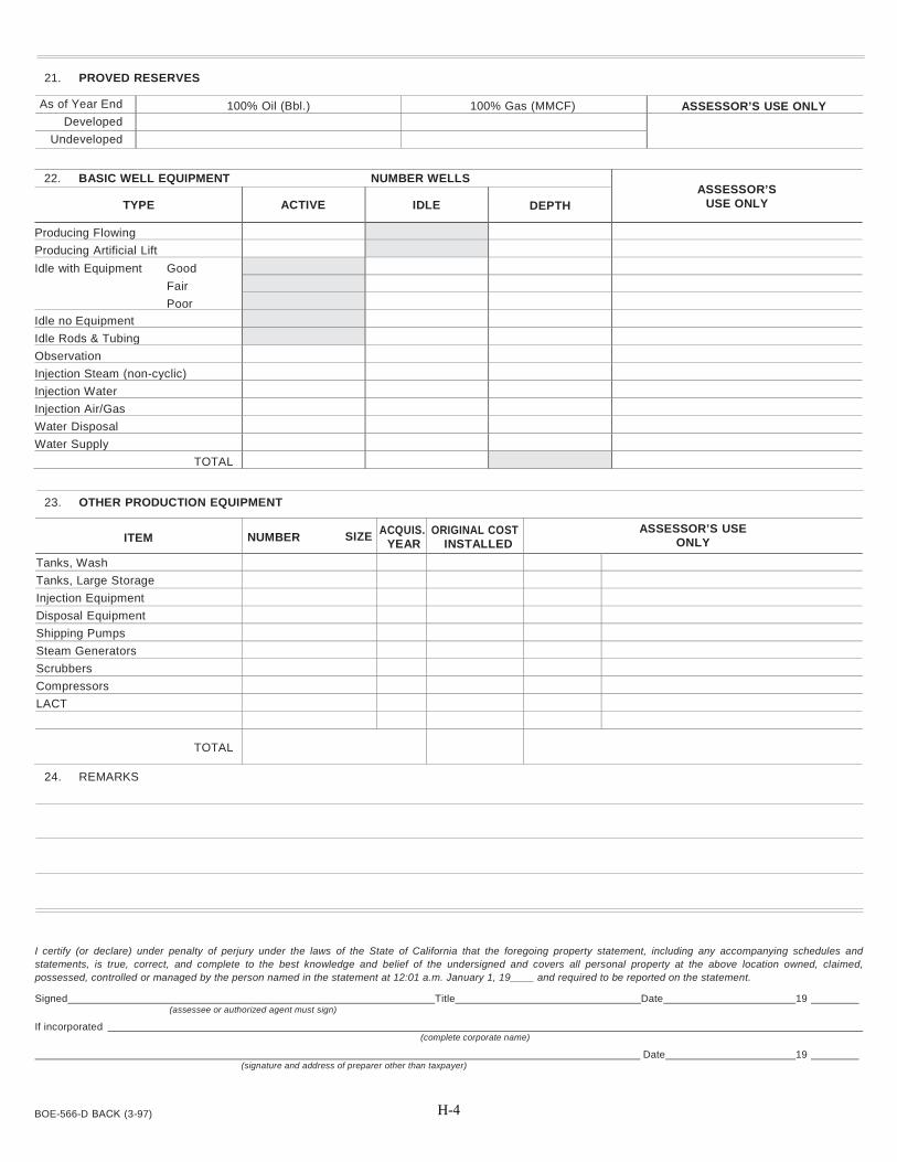
21. PROVED RESERVES

As of Year End 100% Oil (Bbl.) 100% Gas (MMCF) ASSESSOR’S USE ONLY Developed

Undeveloped

22. BASIC WELL EQUIPMENT NUMBER WELLS ASSESSOR’S

USE ONLY TYPE ACTIVE IDLE DEPTH

Producing Flowing Producing Artificial Lift Idle with Equipment Good

Fair Poor

Idle no Equipment Idle Rods & Tubing Observation Injection Steam (non-cyclic) Injection Water Injection Air/Gas Water Disposal Water Supply

TOTAL

23. OTHER PRODUCTION EQUIPMENT

ITEM NUMBER SIZE ACQUIS. YEAR

ORIGINAL COST INSTALLED

ASSESSOR’S USE ONLY

Tanks, Wash Tanks, Large Storage Injection Equipment Disposal Equipment Shipping Pumps Steam Generators Scrubbers Compressors LACT

TOTAL

24. REMARKS

I certify (or declare) under penalty of perjury under the laws of the State of California that the foregoing property statement, including any accompanying schedules and statements, is true, correct, and complete to the best knowledge and belief of the undersigned and covers all personal property at the above location owned, claimed, possessed, controlled or managed by the person named in the statement at 12:01 a.m. January 1, 19____ and required to be reported on the statement.

Signed Title Date 19 (assessee or authorized agent must sign)

If incorporated (complete corporate name)

Date 19 (signature and address of preparer other than taxpayer)

H-4 BOE-566-D BACK (3-97)

INSTRUCTIONS FOR COMPLETING OIL AND DISSOLVED GAS PRODUCTION REPORT

This report is not a public document. The information contained herein will be held secret by the Assessor (Section 451, Revenue and Taxation Code); it can be disclosed only to the district attorney, grand jury and other agencies specified in Section 408 of the Revenue and Taxation Code. Attached schedules are considered to be part of the report. The County Assessor’s failure to keep such records confidential could subject them to civil damages (Government Code Section 1504), and if such failure is determined to be willful, the Assessor may be subjected to other sanctions as provided by law (Government Code Sections 3060 – 3074). Agents of the county hired as consultants are employees of the county and are subject to the same provisions, sanctions and penalties upon failure to keep records confidential.

All personal property owned by the respondent and any property belonging to others on the lease as of January 1 must be reported to the Assessor on the OIL, GAS AND GEOTHERMAL PERSONAL PROPERTY STATEMENT, Form BOE-566-J.

Line numbers listed in these instructions refer to identical line numbers printed on the form. At top of form, fill in the year of lien date for which this report is made.

LINE 1. NAME, MAILING ADDRESS AND PHONE NUMBER

a. NAME OF OPERATOR (PERSON OR CORPORATION)If the name is preprinted, check the spelling and correct any error. In the case of an individual, enter the last name first, thenthe first name and initial. Partnerships should enter at least two names, showing the last name, first name and initial for eachpartner. Corporation names should be complete so they will not be confused with fictitious or DBA names.

b. DBA OR FICTITIOUS NAMEEnter the DBA (Doing Business As) name under which you are operating in this county below the name of the sole owner,partnership or corporation.

c. MAILING ADDRESSEnter the mailing address of the legal entity shown in line 1b above. This may be either a street address or a post office boxnumber. It may differ from the actual location of the property. Include the city, state and ZIP code.

d. PHONE NUMBEREnter the phone number where we may contact you or your authorized representative for information regarding the subjectproperty.

LINE 2. DESCRIPTION OF THE PROPERTY

Report each lease or parcel on a separate report form. Fill in oil field name, lease name and pool, and lease number. Conform to Division of Oil and Gas classification in regard to name of field, lease and pool. Check whether recovery is primary or other type. If other, describe method, for example, waterflood, steam injection (cyclic or flood), fire flood, etc.

LINE 3. PARCEL NUMBER

Fill in the parcel number and tax rate area number, if known.

LINE 4. Submit a separate form for each Department of Energy (DOE) “Formation,” for example, Division of Oil and Gas recognized pool, and label according to the Division of Oil and Gas nomenclature.

LINE 5. Indicate the calendar year for which production is being reported. Report oil (BBLS), water (BBLS) and gas (MCF) production and steam (BBLS) or water (BBLS) injection by months on a calendar year basis and the number or producing or injection wells and days. New wells and/or abandonments should be reported separately.

LINE 9. List the total royalty percent. For leasehold properties check appropriate Box P or G whether the lessor is a private party or a governmental agency and state the government royalty separately.

LINE 13. Report crude oil price per barrel at the end of December before any transportation charges.

LINE 14. Report calendar year’s gas and gas liquids income to the property for working and royalty interests combined (excluding plant’s share of gas and gas liquids).

LINE 15. Report gas (MCF) used as lease fuel.

LINE 16. Report volume of gas (MCF) credited to lease after plant processing. This volume should be the same as that upon which royalty payments are based.

H-5 BOE-566-D INSTRUCTIONS FRONT (3-97)

LINE 17. Report volume of NGL credited to lease after plant processing. This volume should be the same as that upon which royalty payments are based.

LINE 18. Indicate trucking charges per barrel if oil must be hauled.

LINE 21. Indicate your proved developed and undeveloped oil and gas reserves (as defined in S.B.E. Rule 468), as of the year end.

LINE 22. Report the number of wells by type, indicating the status and average depth. Idle with equipment (good, fair, poor), idle no equipment, and idle rods and tubing pertain to producing wells only. A well is considered active if used at least one day during December. Active producers and injectors should equal the number of wells reported for December in the production and injection data. An injector should be reported as a producer if the well was in production at any time during December.

LINE 23. Report additions to or retirements of improvements of your “Other Production Equipment.” The Assessor may, on written notice, request annual reporting of previously existing equipment.

LINE 24. Any other information bearing on the value of the property may be recorded under “Remarks.”

SIGNATURE

This report must be signed by the owner or partner of the business, a duly appointment fiduciary, or an agent. When signed by an agent other than a member of the bar, a certified public accountant, a public accountant, a duly appointed fiduciary or an authorized officer or employee of a corporate assessee or trust company, the assessee’s written authorization of the agent to sign the report on behalf of the assessee should be on file in the Assessor’s office. The entry on the line “Title” should clearly indicate whether or not written authorization is required to be filed with the Assessor.

In the case of a corporation, the report must be signed by an employee or agent whom the board of directors has designated in writing, by name or by title, to sign such report on behalf of the corporation, or by an officer of the corporation. The board of directors may appoint a person or persons to designate such employee or agent. The name of the corporation should be entered on the line provided.

SIGN THE PRODUCTION REPORT IN ACCORDANCE WITH THE REQUIREMENTS LISTED ABOVE. TITLE 18, SECTION 172 OF THE CALIFORNIA CODE OF REGULATIONS PROVIDES THAT REPORTS NOT PROPERLY SIGNED HAVE NOT BEEN PROPERLY SUBMITTED AND THE ASSESSEE MAY BE SUBJECT TO APPLICABLE PENALTIES.

H-6 BOE-566-D INSTRUCTIONS BACK (3-97)

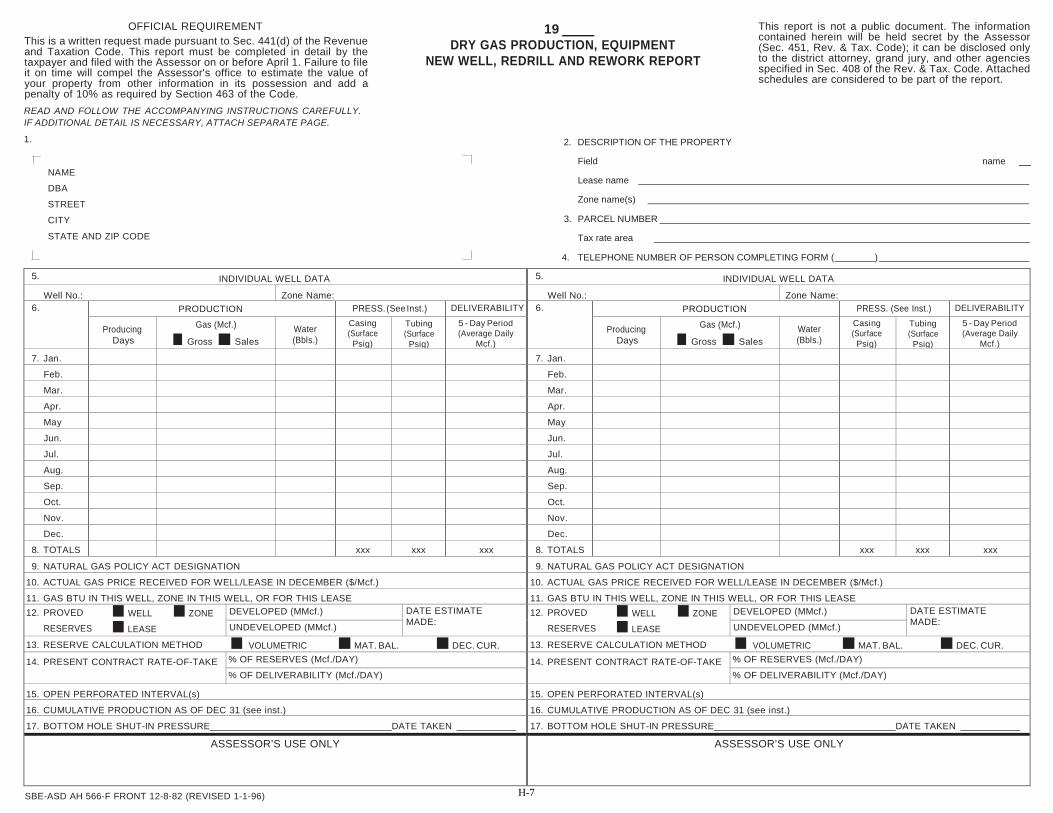
OFFICIAL REQUIREMENT This is a written request made pursuant to Sec. 441(d) of the Revenue and Taxation Code. This report must be completed in detail by the taxpayer and filed with the Assessor on or before April 1. Failure to file it on time will compel the Assessor's office to estimate the value of your property from other information in its possession and add a penalty of 10% as required by Section 463 of the Code. READ AND FOLLOW THE ACCOMPANYING INSTRUCTIONS CAREFULLY. IF ADDITIONAL DETAIL IS NECESSARY, ATTACH SEPARATE PAGE.

1.

19 DRY GAS PRODUCTION, EQUIPMENT

NEW WELL, REDRILL AND REWORK REPORT

2. DESCRIPTION OF THE PROPERTY

This report is not a public document. The information contained herein will be held secret by the Assessor (Sec. 451, Rev. & Tax. Code); it can be disclosed only to the district attorney, grand jury, and other agencies specified in Sec. 408 of the Rev. & Tax. Code. Attached schedules are considered to be part of the report.

NAME

DBA

STREET

CITY

STATE AND ZIP CODE

Field name

Lease name

Zone name(s)

3. PARCEL NUMBER

Tax rate area

4. TELEPHONE NUMBER OF PERSON COMPLETING FORM ( )

5. INDIVIDUAL WELL DATA 5. INDIVIDUAL WELL DATA

Well No.: Zone Name: Well No.: Zone Name: 6. PRODUCTION PRESS. (See Inst.) DELIVERABILITY 6. PRODUCTION PRESS. (See Inst.) DELIVERABILITY

Producing Days

Gas (Mcf.)

■ Gross ■ SalesWater (Bbls.)

Casing (Surface Psig)

Tubing (Surface Psig)

5 - Day Period (Average Daily

Mcf.) Producing

Days

Gas (Mcf.)

■ Gross ■ SalesWater (Bbls.)

Casing (Surface Psig)

Tubing (Surface Psig)

5 - Day Period (Average Daily

Mcf.)

7. Jan. 7. Jan.

Feb. Feb.

Mar. Mar.

Apr. Apr.

May May

Jun. Jun.

Jul. Jul.

Aug. Aug.

Sep. Sep.

Oct. Oct.

Nov. Nov.

Dec. Dec.

8. TOTALS xxx xxx xxx 8. TOTALS xxx xxx xxx

9. NATURAL GAS POLICY ACT DESIGNATION 9. NATURAL GAS POLICY ACT DESIGNATION

10. ACTUAL GAS PRICE RECEIVED FOR WELL/LEASE IN DECEMBER ($/Mcf.) 10. ACTUAL GAS PRICE RECEIVED FOR WELL/LEASE IN DECEMBER ($/Mcf.)

11. GAS BTU IN THIS WELL, ZONE IN THIS WELL, OR FOR THIS LEASE 11. GAS BTU IN THIS WELL, ZONE IN THIS WELL, OR FOR THIS LEASE12. PROVED ■ WELL ■ ZONE

RESERVES ■ LEASE

DEVELOPED (MMcf.) DATE ESTIMATE MADE:

12. PROVED ■ WELL ■ ZONERESERVES ■ LEASE

DEVELOPED (MMcf.) DATE ESTIMATE MADE: UNDEVELOPED (MMcf.) UNDEVELOPED (MMcf.)

13. RESERVE CALCULATION METHOD ■ VOLUMETRIC ■ MAT. BAL. ■ DEC. CUR. 13. RESERVE CALCULATION METHOD ■ VOLUMETRIC ■ MAT. BAL. ■ DEC. CUR.

14. PRESENT CONTRACT RATE-OF-TAKE % OF RESERVES (Mcf./DAY) 14. PRESENT CONTRACT RATE-OF-TAKE % OF RESERVES (Mcf./DAY)

% OF DELIVERABILITY (Mcf./DAY) % OF DELIVERABILITY (Mcf./DAY)

15. OPEN PERFORATED INTERVAL(s) 15. OPEN PERFORATED INTERVAL(s)

16. CUMULATIVE PRODUCTION AS OF DEC 31 (see inst.) 16. CUMULATIVE PRODUCTION AS OF DEC 31 (see inst.)

17. BOTTOM HOLE SHUT-IN PRESSURE DATE TAKEN 17. BOTTOM HOLE SHUT-IN PRESSURE DATE TAKEN

ASSESSOR’S USE ONLY ASSESSOR’S USE ONLY

SBE-ASD AH 566-F FRONT 12-8-82 (REVISED 1-1-96) H-7

18. LEASE SUMMARY

19. GAS USED ON LEASE (Mcf.) 20. LEASE CONDENSATE (Gals.) ($/Gal.)

21. UTILITY SALES LINE PRESSURE (Psig)

22. ROYALTY RATE ■ PRIVATE % ■ GOVERNMENT %

23. IF YOU CHECKED “GOVERNMENT” IN NO. 22, DOES THIS PROPERTY QUALITY FOR A PROPERTY TAX EXEMPTION UNDER R&T CODESECTION 107.2 OR 107.3? ■ YES ■ NO

24. WHO PURCHASES THE GAS PRODUCED ON THIS LEASE?

25. WHAT IS THE CONTRACT EXPIRATION DATE?

26. WHAT IS THE DATE ON WHICH PRICES BECOME RENEGOTIABLE?

27. BASIC WELL EQUIPMENT ASSESSOR’S USE ONLY

Number of Wells

Single Completions

PRODUCING WELLS Dual Completions

Triple CompletionsNON-PRODUCING With Equipment

WELLS No EquipmentDISPOSAL WELLS

TOTALS

28. OTHER PRODUCTION EQUIPMENT ASSESSOR’S USE ONLY

ITEMS Number Size/Description Acquis. Year Original Cost Installed

TANKS, WATER

TANKS, STORAGE

DEHYDRATORS

COMPRESSORS

GATHERING LINES

PIPELINES

DISPOSAL EQUIP.

HEATER

OTHER

TOTAL

29. NEW WELL, REDRILL, REWORK REPORT (see instructions regarding data required.)

WELL NAME AND NUMBER

ZONE NAME

PRODUCING INTERVAL (FEET)

POROSITY (0/ ) (%)

WATER SATURATION (Sw) (%)

COMPRESSIBILITY FACTOR (Z)

DRAINAGE AREA (A) (ACRES)

NET SAND (h) (FEET)

SPECIFIC GRAVITY

FORMATION TEMPERATURE (Tf) (oR)

BOT. HOLE BOT. HOLE BOT. HOLE BOT. HOLE INITIAL FORMATION PRESSURE (PSIG)

SURF. SURF. SURF. SURF. RECOVERY FACTOR (RF) (%)

RESERVOIR MECHANISM

30. REMARKS (Attach additional sheets if needed.)

I certify (or declare) under penalty of perjury under the laws of the State of California that the foregoing production report, including any accompanying schedules and reports, is true, correct, and complete to the best knowledge and belief of the undersigned and covers all production and all property of the kind required to be reported hereon at the above location owned, claimed, possessed, controlled or managed by the person named in the report at 12:01 a.m. January 1, 19 . If prepared by a person other than the taxpayer, his declaration is based on all information of which he has knowledge.

Signed Title ASSESSEE OR AUTHORIZED AGENT MUST SIGN

Date 19

If Incorporated COMPLETE CORPORATE NAME

Date SIGNATURE AND ADDRESS OF PREPARER OTHER THAN TAXPAYER

19

SBE-ASD AH 566-F BACK 12-8-82 (REVISED 1-1-96) H-8

INSTRUCTIONS FOR COMPLETING DRY GAS PRODUCTION, EQUIPMENT, NEW WELL, REDRILL, AND REWORK REPORT

This report is not a public document. The information contained herein will be held secret by the Assessor (Section 451, Revenue and Taxation Code); it can be disclosed only to the district attorney, grand jury, and other agencies specified in Section 408 of the Revenue and Taxation Code. Attached schedules are considered to be part of the report. The County Assessor’s failure to keep such records confidential could subject him to civil damages (Government Code Section 1504), and if such failure is determined to be willful, the Assessor may be subjected to other sanctions as provided by law (Gov- ernment Code Sections 3060-3074). Agents of the county hired as consultants are employees of the county and are sub- ject to the same provisions, sanctions and penalties upon failure to keep records confidential.

If this report is prepared as of a date prior to January 1, any change in real property between the date as of which the report is prepared and January 1, must be reported to the assessor on a supplemental report.

Report each lease or parcel on a separate report form. Two wells may be reported on one form provided the wells do not contain more than one zone. For example if wells A and B produce from single zones, well A would be reported on Lines 5 through 17 on the left side of the form, and well B would be reported on Lines 5 through 17 on the right side of the form. However, if well A produced from two separate and distinct zones, one zone would be reported on the left side of the form, and one zone would be reported on the right.

All personal property owned by the respondent and any property belonging to others on the lease as of January 1 must be reported to the assessor on Form AH 566-D, OIL, GAS, AND GEOTHERMAL PERSONAL PROPERTY STATEMENT. Operating expenses must be reported on Form AH 566-K, ANNUAL OIL AND GAS OPERATING EXPENSE DATA.

Line numbers listed in these instructions refer to identical line numbers printed on the form. At top of form, fill in the year of lien date for which this report is made.

LINE 1. NAME AND MAILING ADDRESS

a. NAME (OF OPERATOR). If the name is preprinted, check the spelling and correct any error. In the case ofan individual, enter the last name first, then the first name and initial. Partnerships should enter at leasttwo names, showing the last name, first name, and initial for each partner. Corporation names should becomplete so they will not be confused with fictitious or DBA names.

b. DBA (FICTITIOUS NAME). Enter the DBA (Doing Business As) name under which you are operating in thiscounty, if applicable, below the name of the sole owner, partnership, or corporation.

c. MAILING ADDRESS. Enter the mailing address of the legal entity shown in Line 1 above. This may be ei-ther a street address or a post office box number. It may differ from the actual location of the property. In-clude the city, state, and ZIP code.

LINE 2. DESCRIPTION OF THE PROPERTY. Report each lease or parcel on a separate report form. Fill in field, lease, and zone names, conforming to Division of Oil and Gas classifications.

LINE 3. PARCEL NUMBER. Enter the parcel number and tax rate area number, if known. If there has been a change in lease boundaries, describe the change on a separate sheet of paper and attach to this report.

LINE 4. TELEPHONE NUMBER. Enter the phone number of the person completing this form so that we may contact you if necessary.

LINE 5. Report individual well data by zone, using as many forms as necessary. Conform to Division of Oil and Gas well numbers and zone nomenclature. All data is for the last full calendar year.

LINES 6-8. Report only nonassociated (dry) gas on this form. Associated (wet) gas is reported on the Oil and Dissolved Gas Production Report.

a. Producing Days refer to the number of days the well produced during the month.

b. Gas (MCF) refers to gross production or production sales in thousand cubic feet produced during themonth. Check the block indicating whether you are reporting gross gas or gas sold. (Gross gas is total gasproduced.)

c. Report water produced (Bbls.).

d. Pressures, both casing and tubing, should be shown monthly for producing gas wells. If a well is not onproduction during the month, shut-in pressures should be shown. All pressures are surface gauge pres-sures.

e. Deliverability refers to tests taken on a well during any month of the year either by the producer himself orby the purchaser. Report the average deliverability over the test period. If test is not over a five dayperiod, explain under Line 30, Remarks. If the test is not for an individual well, but for a group of wells,also explain under Remarks. Report only the latest deliverability test taken for the calendar year.

SBE-ASD AH 566-F INSTRUCTIONS FRONT 12-8-82 (REVISED 1-1-96) H-9

LINE 9. Enter the applicable section of the Natural Gas Policy Act for the well, such as “102”.

LINE 10. Enter the last price received during December of the calendar year being reported for gas produced from this well or lease.

LINE 11. Enter the gas BTU for this well, or zone in this well, if reporting by zone.

LINE 12. Enter the proved reserves in millions of cubic feet for this well, zone, or lease (check proper box) as of December 31 of the calendar year reported. Enter according to the classifications of proved developed and proved undeveloped reserves. If the zone or lease boxes are checked, enter the wells included in the reserve estimate on Line 30, Remarks. Proved reserves are those reserves which geological and engineering informa- tion indicate with reasonable certainty to be recoverable in the future, taking into account reasonably projected physical and economic operating conditions. Present and projected economic conditions shall be determined by reference to all economic factors considered by knowledgeable and informed persons engaged in the operation and buying or selling of such properties, e.g., capitalization rates, product prices and operation expenses.

LINE 13. Check the proper box to show the method used to calculate reserves. If you used some other method to cal- culate reserves, please explain under Remarks, Line 30.

LINE 14. Enter in the respective space, the present contract rate-of-take in MCF/Day depending upon whether the rate is based on a percentage of reserves or deliverability. If the contract-rate-of-take is for a group of wells, so in- dicate under Remarks, Line 30.

LINE 15. Enter the currently open perforated intervals in this well.

LINE 16. Enter the cumulative production of gas for this well, for the zone shown, as of December 31 of the calendar year reported. If you do not have accurate cumulative production, so indicate, showing the beginning date of the cumulative production reported. If data is not available by well, report by zone or lease and so indicate under Remarks, Line 30.

LINE 17. Enter the last bottom hole shut-in pressure available for this zone in this well.

LINE 18. Lease Summary (heading). Do not report data on this line.

LINE 19. Report gas used on lease as fuel.

LINE 20. Report calendar year lease condensate production in gallons, and price per gallon in December.

LINE 21. Enter the pressure of the sales line into which you feed your produced gas.

LINE 22. Indicate the royalty rate percentages paid, both private and government.

LINE 23. If you checked “Government” on Line 22, indicate whether you claim an exemption from property taxes for government royalties under Secs. 107.2 or 107.3 of the Revenue and Taxation Code. Use the Remarks section, Line 30, for further clarification, if necessary.

LINE 24. Enter the name of the purchaser of all of the gas sold from this lease.

LINE 25. Enter the expiration date of your gas sales contract.

LINE 26. Enter the date on which prices become renegotiable.

LINE 27. Basic Well Equipment (heading). This section is for reporting numbers of wells by category in the reporting unit (i.e., lease or parcel).

LINE 28. Other Production Equipment (heading). Report all production equipment on the property. Enter categories of equipment or structures not listed under “other”. Use additional pages if necessary. Complete this section in full detail. For compressors show horsepower, design, and current stages.

LINE 29. This section is to be used to report data for new wells, redrilled wells or reworked wells that require a notifi- cation on a “Notice of Rework” to the California Division of Oil and Gas. Reworks of interest to the assessor are those which permanently alter the well or casing. Data furnished in this section should be the same as that used in making a company reserve estimate. Enclose copies of the following data for each new well, redrill or rework completed during the year being reported.

a. The well completion summary and any subsequent rework history showing the current physical condition ofthe well.

b. The P.G.&E. or company back-pressure test data form for the current producing zone(s) including ananalysis of the gas.

c. One 2" = 100' scale IES log and a copy of the sonic, density or any other evaluation log run.

d. For directionally drilled wells, a directional survey.

The taxpayer may optionally file any other additional information that is germane to the assessment function such as geo- logic structure maps, estimates of water influx and, for new wells, estimated date of pipeline connection.

SBE-ASD AH 566-F INSTRUCTIONS BACK 12-8-82 (REVISED 1-1-96) H-10

Year of

Acq.

Year of

Mfr.

Description and Lease or Identification

Number

Cost to Purchase

New

TOTAL FULL VALUE

OFFICIAL REQUIREMENT

A report on this form is required of you by Sec- tion 441 of the Revenue and Taxation Code. The statement must be completed according to the instructions and filed with the Assessor on or before April 1. Failure to file it on time will compel the Assessor's office to estimate the value of your property from other information in its possession and add a penalty of 10% as required by Section 463 of the Code.

19 OIL, GAS AND GEOTHERMAL

PERSONAL PROPERTY STATEMENT

This statement is not a public document. The information contained herein will be held secret by the Assessor (Sec. 451, Rev. & Tax. Code); it can be disclosed only to the district attorney, grand jury, and other agencies specified in Sec. 408 of the Rev. & Tax. Code. Attached sched- ules are considered to be part of the statement.

READ AND FOLLOW THE INSTRUCTIONS ON THE REVERSE SIDE

1.

NAME

DBA

STREET

CITY

STATE AND ZIP CODE

2. LOCATION OF THE PROPERTY:

(a separate report must be filed for each property)

FIELD NAME

LEASE NAME AND POOL

3. PARCEL NUMBER

TAX RATE AREA

4. PHONE NUMBER

PERSONAL PROPERTY ASSESSOR’S USE ONLY

FULL VALUE

5. Supplies (fuel) Type: Gravity: Barrels:

Items Acquis. Year

Original Cost

6. Office furniture

7. Warehouse stock (parts, tools, equipment, etc.)

8. Yard stock (rods, tubing, casing, etc.)

9. Other (chemicals, unlicensed vehicles, etc.)

10. DECLARATION OF PROPERTY BELONGING TO OTHERS — IF NONE WRITE "NONE"(SPECIFY TYPE BY CODE NUMBER)

Report conditional sales contracts in lines 6-9 as applicable 1. Leased Equipment 4. Vending Equipment ▼ 2. Leased-Purchase Option Equipment 5. Other businesses3. Capitalized Leased Equipment 6. Government-Owned Property

Tax Obligation: A. Lessor B. Lessee

Annual Rent

▼ Lessor's Name Mailing Address

Lessor's Name Mailing Address

11. Remarks

I certify (or declare) under penalty of perjury under the laws of the State of California that the foregoing property statement, including any accompanying schedules and statements, is true, correct, and complete to the best knowledge and belief of the undersigned and covers all personal property at the above location owned, claimed, possessed, controlled or managed by the person named in the statement at 12:01 a.m. January 1, 19____ and required to be reported on the statement.

Signed Title Date 19 (assessee or authorized agent must sign)

If incorporated (complete corporate name)

Date 19 (signature and address of preparer other than taxpayer)

BOE-566-J FRONT (3-97) H-11

INSTRUCTIONS FOR COMPLETING THE OIL, GAS AND GEOTHERMAL PERSONAL PROPERTY STATEMENT

Report all personal property owned by the respondent and any property belonging to others on the lease as of January 1.

Line numbers listed in these instructions refer to identical line numbers printed on the form.

LINE 1. NAME AND MAILING ADDRESS a. NAME OF OPERATOR (PERSON OR CORPORATION)

If the name is preprinted, check the spelling and correct any error. In the case of an individual, enter the last name first, then the firstname and initial. Partnerships should enter at least two names, showing the last name, first name and initial for each partner.Corporation names should be complete so they will not be confused with fictitious or DBA names.

b. DBA OR FICTITIOUS NAMEEnter the DBA (Doing Business As) name number which you are operating in this county below the name of the sole owner,partnership, or corporation.

c. MAILING ADDRESSEnter the mailing address of the legal entity shown in line 1a above. This may be either a street address or a post office box number.It may differ from the actual location of the property. Include the city, state and ZIP code.

LINE 2. LOCATION OF THE PROPERTY

Fill in the lease and field name. Conform to State Division of Oil and Gas classification in regard to names of fields and pools. For geothermal properties, ignore term "pool," and fill in "operating unit" if this term applies.

LINE 3. PARCEL NUMBER

Fill in the parcel number and tax rate area number, if known.

LINE 4. PHONE NUMBER Enter the phone number where we may contact you or your authorized representative for information regarding the subject property.

LINE 5. SUPPLIES (Used as fuel)

Enter the type of fuel, A.P.I. gravity and the number of barrels.

LINES 6 OFFICE EQUIPMENT, WAREHOUSE STOCK, YARD STOCK, OTHER thru 9. Enter the year acquired, if known, the cost, and a description sufficient to identify the property.

LINE 10. DECLARATION OF PROPERTY BELONGING TO OTHERS

If property belonging to others, or their business entities, is located on your premises, report the owner's name and mailing address. If it is leased equipment, read your agreement carefully and enter the type by Code and whether A. Lessor or B. Lessee has the tax obligation. For assessment purposes, the Assessor will consider, but is not bound to, the contractual agreement.

1. LEASED EQUIPMENT. Report the year of acquisition, the year of manufacture, description of the leased property, the leasecontract number or other identification number, the total installed cost to purchase (including sales tax), and the annual rent; do notinclude in lines 6-9. (See No. 3, below)

2. LEASE-PURCHASE OPTION EQUIPMENT. Report here all equipment acquired on lease-purchase option on which the finalpayment remains to be made. Enter the year of acquisition, the year of manufacture, description of the leased property, the leasecontract number or other identification number, the total installed cost to purchase (including sales tax), and the annual rent. If finalpayment has been made, report full cost in lines 6-9, as applicable. (See No. 3, below)

3. CAPITALIZED LEASE EQUIPMENT. Report here all leased equipment that has been capitalized at the present value of theminimum lease payments on which a final payment remains to be made. Enter the year of acquisition, the year of manufacture,description of the leased property, the lease contract number or other identification number, and the total installed cost to purchase(including sales tax). Do not include in lines 6-9 unless final payment has been made.

4. VENDING EQUIPMENT. Report the model and description of the equipment; do not include in lines 6-9.5. OTHER BUSINESSES. Report other businesses on your premises.

6. GOVERNMENT-OWNED PROPERTY. If you possess or use government-owned land, improvements, or fixed equipment, orgovernment-owned property is located on your premises, report the name and address of the agency which owns the property, anda description of the property.

SIGNATURE

This statement must be signed by the owner or partner of the business, a duly appointed fiduciary, or an agent. When signed by an agent other than a member of the bar, a certified public accountant, a public accountant, a duly appointed fiduciary or an authorized officer or employee of a corporate assessee or trust company, the assessee's written authorization of the agent to sign the statement on behalf of the assessee should be on file in the Assessor's office. The entry on the line "title" should clearly indicate whether or not written authorization is required to be filed with the Assessor. In the case of a corporation, the property statement must be signed by an employee or agent whom the board of directors has designated in writing, by name or by title, to sign such statements on behalf of the corporation, or by an officer of the corporation. The board of directors may appoint a person or persons to designate such employee or agent. The name of the corporation should be entered on the line provided.

BOE-566-J BACK (3-97) H-12

OFFICIAL REQUIREMENT

This is a written request made pursuant to Sec. 441(d) of the Revenue and Taxation Code. This report must be completed in detail by the tax- payer and filed with the Assessor’s office as requested on or before April 1. Failure to file it on time will compel the Assessor’s office to estimate the value of your property from other information in its possession and add a penalty of 10% as required by Section 463 of the Code.

READ THE ATTACHED INSTRUCTIONS

19 ANNUAL OIL AND GAS OPERATING EXPENSE

DATA

BEFORE COMPLETING THE FORM. This statement is not a public document. The information contained herein will be held secret by the Assessor (Sec. 451, Rev. & Tax. Code); it can be disclosed only to the district attorney, grand jury, and other agencies specified in Sec. 408 of the Rev. & Tax. Code. Attached sched- ules are considered to be part of the statement.

1. Name and Mailing Address (make necessary corrections)

PERSON OR CORPORATION NAME DBA MAILING ADDRESS CITY, STATE and ZIP CODE

PHONE NUMBER

2. DESCRIPTION OF THE PROPERTY:(a separate report must be filed for each property)Field nameLease name and poolRECOVERY: ■ PRIMARY ■ OTHER(DESCRIBE)

3. PARCEL NUMBERTax rate area

WELL DATA: ASSESSOR’S USE

ONLY 4. Number of Producing Wells X X X X 5. Average Tubing Depth, feet X X X X 6. Production X X X X X X X X

a. Crude oil (BBLS) X X X X b. Water (BBLS) X X X X c. Gas (MCF) X X X X

FIELD OPERATING EXPENSES: ASSESSOR’S USE

ONLY 7. Labor (including employee benefits) $ 8. Materials and Supplies (expensed items only)9. Well Maintenance (pulling, bailing, etc.)

10. Contract Work and Rentals11. Insurance12. Utilities13. Compression Services14. Transportation (except crude oil hauling)15. Dehydration and Waste Water Disposal16. Enhanced Recovery Costs X X X X

a. Fuel Type Barrels/MCF X X X X 1. Purchased $ X X X X 2. Lease Products X X X X

b. Water X X X X X X X X c. Chemicals X X X X X X X X X X X X d. Maintenance & Repairs X X X X X X X X X X X X

Total Enhanced Recovery Costs $ 17. Overhead (direct-field or district)18. Other (fully explain on attached sheet)19. TOTAL FIELD OPERATING EXPENSES $

H-13SBE-ASD AH 566-K FRONT 7-31-80 (REVISED 3-13-96)

CAPITAL EXPENDITURES: ASSESSOR’S USE ONLY

20. New Wells

Well Number Well Type Date Completed Depth Cost

$ X X X X X X X X X X X X

Total New Well Cost $

21. Remedial Well Work

Well Number Well Type Date Completed Depth Cost

$ X X X X X X X X X X X X

Total Remedial Well Work Cost $

22. Abandonments

Well Number Well Type Date Abandoned Depth Cost Salvage Value

$ $ X X X X X X X X X X X X

Total Abandonment Cost (net) $

23. Surface Investment

Type Cost $ X X X X

X X X X X X X X

Total Surface Investment $

24. Work In Progress

Actual/Estimate Cost Fixed Plant, Equipment, & Other $ Wells Non-Fixture & Fixture $

Total Improvement $ Moveable Equipment $

25. Other (fully explain on attached sheet) $

26. TOTAL CAPITAL EXPENDITURES $

27. REMARKS

I certify (or declare) under penalty of perjury under the laws of the State of California that the foregoing expense data statement, including any accompanying schedules and statements, is true, correct, and complete to the best knowledge and belief of the under- signed and covers all property and only those expenses of the kind to be reported hereon at the above location owned, claimed, possessed, controlled or managed by the person named in the report at 12:01 a.m. on January 1, 19 .

Signed Title Date 19 (assessee or authorized agent must sign)

If Incorporated (complete corporate name)

Date 19 (signature and address of preparer other than taxpaper)

SBE-ASD AH 5 566-K BACK 7-31-80 (REVISED 3-13-96)H-14

INSTRUCTIONS FOR COMPLETING THE OIL AND GAS OPERATING EXPENSE DATA REPORT

Line numbers listed in these instructions refer to identical line numbers printed on the form.

LINE 1. DATE, NAME, MAILING ADDRESS AND PHONE NUMBER a. At top of form: Fill in the year of the lien date for which this expense report is made.

b. NAME OF OPERATOR (PERSON OR CORPORATION)If the name is preprinted, check the spelling and correct any error. In the case of an individual,enter the last name first, then the first name and initial. Partnerships should enter at least twonames, showing the last name, first name, and initial for each partner. Corporation namesshould be complete so they will not be confused with fictitious or DBA names.

c. DBA OR FICTITIOUS NAMEEnter the DBA (Doing Business As) name under which you are operating in this countybelow the name of the sole owner, partnership, or corporation.

d. MAILING ADDRESSEnter the mailing address of the legal entity shown in line 1b above. This may be either astreet address or a post office box number. It may differ from the actual location of theproperty. Include the city, state, and ZIP code.

e. PHONE NUMBEREnter the phone number where we may contact you or your authorized representative forinformation regarding the subject property.

LINE 2. DESCRIPTION OF THE PROPERTY Report each property or parcel on a separate report form. Fill in field name, lease name and pool. Conform to Division of Oil and Gas classification in regard to name of field, pool, and zone. Check whether recovery is primary or other type. If other, describe method [for example, water- flood, steam injection (cyclic or flood), fire flood, etc.].

LINE 3. PARCEL NUMBER Fill in the parcel number and tax rate area number, if known.

LINE 4. Producing wells reported are those wells which actually contribute to normal lease production on a profitable basis.

LINE 6. Production is to be for the same period as used for the reporting of the expense data on this form.

LINES 7 Report direct field operating expenses only. Do not report capitalized items or royalty payments on thru 15. these lines.

LINE 16. Report costs related to enhanced recovery only on this line. Use line 12 for all utility costs not associated with enhanced recovery operations.

LINES 17 Report direct field operating expenses only. Do not report capitalized items or royalty payments on thru 19. these lines.

LINES 20 Report the well number, well type (for example, producing, pumping, injection steam, observation, and 21. water source), date completed, depth and total cost (tangible and intangible) for each well. Report

the summation of the costs for each line. Report on these lines all work that required a Division of Oil and Gas permit.

LINE 22. Report the well number, well type (for example, producing, pumping, injection steam, observation, water source), date abandoned, well depth, total cost, and salvage value for each well abandoned. For the Total Abandonment Cost (Net) entry, report the total cost less any salvage from the wells.

SBE-ASD AH 566-K INSTRUCTIONS FRONT 7-31-80 (REVISED 3-13-96) H-15

LINE 23. Report amounts capitalized for surface investment (for example, steam generators, buildings, product handling equipment, and vapor recovery systems).

LINE 24. Report expenditures for projects not yet completed for intended use differentiating moveable equip- ment, wells, and fixed plant and facilities. Indicate whether the amounts reported are actual or estimated.

LINE 25. Report all other investment expenditures not listed in lines 20 thru 24.

Crude Hauling. Report expenses on line 18 if oil “must” be hauled. Fully explain on attached sheet.

DO NOT INCLUDE DEPRECIATION, DEPLETION, AMORTIZATION, INTEREST, FEDERAL AND STATE INCOME TAXES, PROPERTY TAXES, ROYALTY PAYMENTS, AND GENERAL OFFICE OVERHEAD.

SIGNATURE

This report must be signed by the owner or partner of the business, a duly appointed fiduciary, or an agent. When signed by an agent other than a member of the bar, a certified public accountant, a public accountant, a duly appointed fiduciary or an authorized officer or employee of a corporate assessee or trust company, the assessee’s written authorization of the agent to sign the report on behalf of the assessee should be on file in the Assessor’s office. The entry on the line “title” should clearly indicate whether or not written authorization is required to be filed with the Assessor.

In the case of a corporation, the report must be signed by an employee or agent whom the board of directors has designated in writing, by name or by title, to sign such reports on behalf of the corporation, or by an officer of the corporation. The board of directors may appoint a person or persons to designate such employee or agent. The name of the corporation must be entered on the line provided.

SIGN THE PRODUCTION REPORT IN ACCORDANCE WITH THE REQUIREMENTS LISTED ABOVE. TITLE 18, SECTION 172 OF THE CALIFORNIA CODE OF REGULATIONS PROVIDES THAT REPORTS NOT PROPERLY SIGNED HAVE NOT BEEN PROPERLY SUBMITTED AND THE ASSESSEE MAY BE SUBJECT TO APPLICABLE PENALTIES.

H- 16 SBE-ASD AH 566-K INSTRUCTIONS BACK 7-31-80 (REVISED 3-13-96)

APPENDIX I: SELECTED STATUTES AND PROPERTY TAX RULES

REVENUE AND TAXATION CODE51. Adjustments to base year values. (a) For purposes of subdivision (b) of Section 2 ofArticle XIII A of the California Constitution, for each lien date after the lien date in which the base year value is determined pursuant to Section 110.1, the taxable value of real property shall, except as otherwise provided in subdivision (b) or (c), be the lesser of:

(1) Its base year value, compounded annually since the base year by an inflation factor, which shall be determined as follows:

(A) For any assessment year commencing prior to January 1, 1985, the inflation factor shall be the percentage change in the cost of living, as defined in Section 2212.

(B) For any assessment year commencing after January 1, 1985, the inflation factor shall be the percentage change from December of the prior fiscal year to December of the current fiscal year in the California Consumer Price Index for all items, as determined by the California Department of Industrial Relations. In no event shall the percentage increase for any assessment year determined pursuant to subparagraph (A) or (B) exceed 2 percent of the prior year's value.

(2) Its full cash value, as defined in Section 110, as of the lien date, taking into account reductions in value due to damage, destruction, depreciation, obsolescence, removal of property, or other factors causing a decline in value.

(b) If the real property was damaged or destroyed by disaster, misfortune, or calamity and the board of supervisors of the county in which the real property is located has not adopted an ordinance pursuant to Section 170, or any portion of the real property has been removed by voluntary action by the taxpayer, the taxable value of the property shall be the sum of the following:

(1) The lesser of its base year value of land determined under paragraph (1) of subdivision (a) or full cash value of land determined pursuant to paragraph (2) of subdivision (a).

(2) The lesser of its base year value of improvements determined pursuant to paragraph (1) of subdivision (a) or the full cash value of improvements determined pursuant to paragraph (2) of subdivision (a).

The sum determined under this subdivision shall then become the base year value of the real property until that property is restored, repaired, or reconstructed or other provisions of law require establishment of a new base year value.

(c) If the real property was damaged or destroyed by disaster, misfortune or calamity and the board of supervisors in the county in which the real property is located has adopted an ordinance pursuant to Section 170, the taxable value of the real property shall be its assessed value as computed pursuant to Section 170.

(d) For purposes of this section, "real property" means that appraisal unit that persons in the marketplace commonly buy and sell as a unit, or that is normally valued separately.

AH 566 I–1 August 1996

(e) Nothing in this section shall be construed to require the assessor to make an annual reappraisal of all assessable property. However, for each lien date after the first lien date for which the taxable value of property is reduced pursuant to paragraph (2) of subdivision (a), the value of that property shall be annually reappraised at its full cash value as defined in Section 110 until that value exceeds the value determined pursuant to paragraph (1) of subdivision (a). In no event shall the assessor condition the implementation of the preceding sentence in any year upon the filing of an assessment appeal.

61. "Change in ownership" includes. Except as otherwise provided in Section 62, change inownership, as defined in Section 60, includes, but is not limited to:

(a) The creation, renewal, sublease, assignment, or other transfer of the right to produce or extract oil, gas, or other minerals regardless of the period during which the right may be exercised. The balance of the property, other than the mineral rights, shall not be reappraised pursuant to this section.

(b) The creation, renewal, extension, sublease, or assignment of a taxable possessory interest in tax exempt real property for any term. For purposes of this subdivision, "renewal" and "extension" do not include the granting of an option to renew or extend an existing agreement pursuant to which the term of possession of the existing agreement would, upon exercise of the option, be lengthened, whether the option is granted in the original agreement or subsequent thereto.

(c) (1) The creation of a leasehold interest in taxable real property for a term of 35 years or more (including renewal options), the termination of a leasehold interest in taxable real property which had an original term of 35 years or more (including renewal options), and any transfer of a leasehold interest having a remaining term of 35 years or more (including renewal options); or (2) any transfer of a lessor's interest in taxable real property subject to a lease with a remaining term (including renewal options) of less than 35 years.

Only that portion of a property subject to that lease or transfer shall be considered to have undergone a change of ownership.

For the purpose of this subdivision, for 1979-80 and each year thereafter, it shall be conclusively presumed that all homes eligible for the homeowners' exemption, other than manufactured homes located on rented or leased land and subject to taxation pursuant to Part 13 (commencing with Section 5800), that are on leased land have a renewal option of at least 35 years on the lease of that land, whether or not in fact that renewal option exists in any contract or agreement.

(d) The creation, transfer, or termination of any joint tenancy interest, except as provided in subdivision (f) of Section 62, and in Section 63 and in Section 65.

(e) The creation, transfer, or termination of any tenancy-in-common interest, except as provided in subdivision (a) of Section 62 and in Section 63.

(f) Any vesting of the right to possession or enjoyment of a remainder or reversionary interest which occurs upon the termination of a life estate or other similar precedent property interest, except as provided in subdivision (d) of Section 62 and in Section 63.

AH 566 I–2 August 1996

(g) Any interests in real property which vest in persons other than the trustor (or, pursuant to Section 63, his or her spouse) when a revocable trust becomes irrevocable.

(h) The transfer of stock of a cooperative housing corporation, vested with legal title to real property that conveys to the transferee the exclusive right to occupancy and possession of that property, or a portion thereof. A "cooperative housing corporation" is a real estate development in which membership in the corporation, by stock ownership, is coupled with the exclusive right to possess a portion of the real property.

(i) The transfer of any interest in real property between a corporation, partnership, or other legal entity and a shareholder, partner, or any other person.

75. Legislative intent. It is the intent of the Legislature in enacting this chapter to fullyimplement Article XIII A of the California Constitution and to promote increased equity among taxpayers by enrolling and making adjustments of taxes resulting from changes in assessed value due to changes in ownership and completion of new construction at the time they occur. The Legislature finds and declares that under the law in effect prior to the enactment of this chapter, recognition of these increases is delayed from four to 16 months, which results in an unwarranted reduction of taxes for some taxpayers with a proportionate and inequitable shift of the tax burden to other taxpayers.

It is also the intent of the Legislature that the provisions of this chapter shall be limited to assessments on the supplemental roll which are authorized by the provisions of this chapter and none of its provisions shall be applied, construed, or used as a basis for interpreting legislative intent when determining the effect of any other provision of this division. The Legislature finds and declares that the supplemental assessment system created by this chapter involves practical tax administration considerations which require unique solutions. Except as expressly provided in Article 2.5 (commencing with Section 75.18), these solutions are not appropriate to the general assessment of property under the provisions of Chapter 3 (commencing with Section 401) of Part 2 and the adoption of the supplemental roll assessment system is not intended to affect the valuation or assessment provisions applicable to the regular assessment roll.

75.1. Application. Except where the context or the specific provisions of this chapter otherwise require, all of the following apply:

(a) The definitions in this article govern the construction of this chapter.

(b) The other provisions of this division apply to assessments made pursuant to this chapter.

(c) The taxes due pursuant to this chapter are in addition to any other taxes due under this division.

75.2. "Current roll." "Current roll" means the roll for the fiscal year during which the change in ownership occurs or the new construction is completed.

AH 566 I–3 August 1996

75.3. "The roll being prepared." "The roll being prepared" means the roll for the fiscal year following the fiscal year in which the change in ownership occurs or the new construction is completed.

75.4. "Current tax rate." "Current tax rate" means the tax rate applicable to the current roll, including any rate in excess of the limitation prescribed by subdivision (a) of Section 1 of Article XIII A of the California Constitution.

75.5. "Property." "Property" means and includes real property, other than fixtures which are normally valued as a separate appraisal unit from a structure, and manufactured homes subject to taxation under Part 13 (commencing with Section 5800).

75.6. "Fiscal year." "Fiscal year" means a fiscal year beginning July 1 and ending June 30.

75.7. "Supplemental roll." "Supplemental roll" means the roll prepared or amended in accordance with the provisions of this chapter and containing properties which have changed ownership or had new construction completed.

75.8. "New base year value." "New base year value" means the full cash value of property on the date it changes ownership or of new construction on the date it is completed.

75.9. "Taxable value." "Taxable value" means the base year full value adjusted for any given lien date as required by law or the full cash value for the same date, whichever is less. In the case of real property which, prior to the date of the change in ownership or completion of new construction, was assessed by the board pursuant to Section 19 of Article XIII of the California Constitution, "taxable value" means that portion of the state-assessed value determined by the board to be properly allocable to the property which is subject to the supplemental assessment.

75.10. New base year value. (a) Commencing with the 1983-84 assessment year and each assessment year thereafter, whenever a change in ownership occurs or new construction resulting from actual physical new construction on the site is completed, the assessor shall appraise the property changing ownership or the new construction at its full cash value (except as provided in Section 68 and subdivision (b) of this section) on the date the change in ownership occurs or the new construction is completed. The value so determined shall be the new base year value of the property or the new construction.

AH 566 I–4 August 1996

(b) For purposes of this chapter, "actual physical new construction" includes the removal of a structure from land. The new base year value of the remaining property (after the removal of the structure) shall be determined in the same manner as provided in subdivision (c) of Section 51.

(c) For purposes of this section, "actual physical new construction" includes the discovery of previously unknown reserves of oil or gas.

Text of section operative January 1, 1997.1

75.11. Supplemental assessments. (a) If the change in ownership occurs or the new construction is completed on or after January 1 but on or before May 31, then there shall be two supplemental assessments placed on the supplemental roll. The first supplemental assessment shall be the difference between the new base year value and the taxable value on the current roll. In the case of a change in ownership of the full interest in the real property, the second supplemental assessment shall be the difference between the new base year value and the taxable value to be enrolled on the roll being prepared. If the change in ownership is of only a partial interest in the real property, the second supplemental assessment shall be the difference between the sum of the new base year value of the portion transferred plus the taxable value on the roll being prepared of the remainder of the property and the taxable value on the roll being prepared of the whole property. For new construction, the second supplemental assessment shall be the value change due to the new construction.

(b) If the change in ownership occurs or the new construction is completed on or after June 1 but before the succeeding January 1, then the supplemental assessment placed on the supplemental roll shall be the difference between the new base year value and the taxable value on the current roll.

(c) If there are multiple changes in ownership or multiple completions of new construction, or both, with respect to the same real property during the same assessment year, then there shall be a net supplemental assessment placed on the supplemental roll, in addition to the assessment pursuant to subdivision (a) or (b). The net supplemental assessment shall be the most recent new base year value less the sum of (1) the previous entry or entries placed on the supplemental roll computed pursuant to subdivision (a) or (b), and (2) the corresponding taxable value on the current roll or the taxable value to be entered on the roll being prepared, or both, depending on the date or dates the change of ownership occurs or new construction is completed as specified in subdivisions (a) and (b).

(d) No supplemental assessment authorized by this section shall be valid, or have any force or effect, unless it is placed on the supplemental roll on or before the applicable date specified in paragraph (1) or (2), as follows:

1 A 1995 law (Section 21 of Stats.1995, Ch.499) provides that the change in the property tax lien date made by that act shall apply with respect to the January 1, 1997 lien date and each lien date thereafter. This note is applicable to Sections 75.12, 75.18, and 75.31 herein. See Revenue and Taxation Code Sections 75 et seq. for further changes and for provisions operative through December 31, 1996.

AH 566 I–5 August 1996

(1) The fourth July 1 following the July 1 of the assessment year in which either a statement reporting the change in ownership was filed pursuant to Section 480, 480.1, or 480.2, a preliminary change in ownership report was filed pursuant to Section 480.3, or the new construction was completed.

(2) The sixth July 1 following the July 1 of the assessment year in which either a statement reporting the change in ownership was filed pursuant to Section 480, 480.1, or 480.2, a preliminary change in ownership report was filed pursuant to Section 480.3, or the new construction was completed, if the penalty provided for in Section 504 is added to the assessment.

For the purposes of this subdivision, "assessment year" means the period beginning annually as of 12:01 a.m. on the first day of January and ending immediately prior to the succeeding first day of January. No limitations period specified in paragraph (1) or (2) shall commence unless the filing or transmittal specified in the relevant paragraph has been completed.

(e) If, before the expiration of the applicable period specified in subdivision (d) for making a supplemental assessment, the taxpayer and the assessor agree in writing to extend the period for making a supplemental assessment, correction, or claim for refund, a supplemental assessment may be made at any time prior to the expiration of that extended period. The extended period may be further extended by successive written agreements entered into prior to the expiration of the most recent extension.

Text of section operative January 1, 1997.

75.12. New construction; notice to assessor. (a) For the purposes of this chapter, new construction shall be deemed completed on the earliest of the following dates:

(1) The date upon which the new construction is available for use by the owner, unless the owner does not intend to occupy or use the property. The owner shall notify the assessor prior to, or within 30 days of, the date of commencement of construction that he or she does not intend to occupy or use the property. If the owner does not notify the assessor as provided in this subdivision, the date shall be conclusively presumed to be the date of completion.

(2) If the owner does not intend to occupy or use the property, the date the property is occupied or used with the owner's consent.

(3) If the property cannot be functionally used or occupied on the date it is available for use considering the type of property and any special facts and circumstances affecting use or occupancy, the date the property can be functionally used or occupied.

(b) For the purposes of this section:

(1) "Occupy or use" means the occupancy or use by the owner, including the rental or lease of the property, except as provided in paragraph (2).

AH 566 I–6 August 1996

(2) Property shall not be considered occupied or used by the owner or with the owner's consent if the occupancy or use is incidental to an offer for a change of ownership, including, but not limited to, use of the property as a model home.

(c) The board, after consultation with the California Assessors Association, shall adopt rules and regulations defining the date of completion of new construction in accordance with this section. The rules and regulations shall not define the date of completion in a manner that the date of completion of all new construction is postponed until the following lien date.

(d) Nothing in this section shall preclude the reassessment of that property on the assessment roll for January 1 following the date of completion.

(e) The owner of any property who notifies the assessor pursuant to subdivision (a) that he or she does not intend to occupy or use the property shall notify the assessor within 45 days of the earliest date that any of the following occur:

(1) The property changes ownership pursuant to an unrecorded contract of sale.

(2) The property is leased or rented.

(3) The property is occupied or used by the owner for any purpose other than provided in subdivision (b).

(4) The property is occupied or used with the owner's consent for any purpose other than provided in subdivision (b).

(f) The failure to provide the assessor the notice required by subdivision (e), whether requested or not, shall result in a penalty in the amount specified in Section 482.

75.13. Supplemental assessment not an escape assessment. Any supplemental assessment shall not be deemed to be an escaped assessment subject to Section 4837.5.

75.14. Supplemental assessment; limitation. A supplemental assessment pursuant to this chapter shall not be made for any property not subject to the assessment limitations of Article XIII A of the California Constitution. All property subject to the assessment limitations of Article XIII A of the California Constitution shall be subject to the provisions of this chapter, except as otherwise provided in this article.

Text of section operative January 1, 1997.

75.15. Taxable fixtures. (a) For fixtures, other than fixtures that are included in a change in ownership or that are included in a structure and are assessed at the completion of the new construction of a structure pursuant to Section 75.12, taxpayers shall report to the assessor once each year at the time the annual property statement is due, on the fixtures added to real property and fixtures removed from real property, the dates of those additions and removals, and the cost of each in the applicable period as follows:

(1) In 1997, the prior 10-month period from March 1 to January 1.

AH 566 I–7 August 1996

(2) In 1998 and each year thereafter, the prior 12-month period from January 1 to January 1.

This reporting requirement shall not apply to fixtures added or removed on or after the first day of the month following the effective date of the act adding this sentence to this subdivision. One supplemental tax bill shall be prepared for those fixtures based on the cost of the fixtures added and subtracted from real property, the date of each addition or subtraction, and the appropriate tax rate computed pursuant to Section 75.41.

The taxes due from the resulting tax bill shall be collected in the same manner and at the same times as other supplemental tax bills mailed on the same date.

(b) For the purposes of the supplemental roll, taxpayers shall report pursuant to this section only those fixtures which are taxable on the supplemental roll.

(c) This section shall become operative on March 1, 1987.

Text of section operative January 1, 1997.

75.18. Application of inflation rate. On and after July 1, 1997, if the actual date of the most recent change in ownership or completion of new construction entered on the supplemental roll occurs between January 1 and June 30, then the new base year value shall be adjusted on the January 1 following the change in ownership or completion of new construction by the inflation factor, which shall be determined as provided in subdivision (a) of Section 51.

Text of section operative January 1, 1997.

75.31. Notice to assessee. (a) Whenever the assessor has determined a new base year value as provided in Section 75.10, the assessor shall send a notice to the assessee showing the following:

(1) The new base year value of the property that has changed ownership, or the new base year value of the completed new construction that shall be added to the existing taxable value of the remainder of the property.

(2) The taxable value appearing on the current roll, and if the change in ownership or completion of new construction occurred between January 1 and May 31, the taxable value on the roll being prepared.

(3) The date of the change in ownership or completion of new construction.

(4) The amount of the supplemental assessments.

(5) The exempt amount, if any, on the current roll or the roll being prepared.

(6) The date the notice was mailed.

(7) A statement that the supplemental assessment was determined in accordance with Article XIII A of the California Constitution that generally requires reappraisal of property whenever a change in ownership occurs or property is newly constructed.

(8) Any other information which the board may prescribe.

AH 566 I–8 August 1996

(b) In addition to the information specified in subdivision (a), the notice shall inform the assessee of the procedure for filing a claim for exemption that is to be filed within 30 days of the date of the notice.

(c) The notice shall advise the assessee of the right to an informal review and the right to appeal the supplemental assessment, and, unless subject to subdivision (d), that the appeal must be filed within 60 days of the date of the notice. For the purposes of equalization proceedings, the supplemental assessment shall be considered an assessment made outside of the regular assessment period as provided in Section 1605.

(d) For counties in which the board of supervisors has adopted the provisions of subdivision (c) of Section 1605, the notice shall advise the assessee of the right to appeal the supplemental assessment, and that the appeal must be filed within 60 days of the date of the mailing of the tax bill. For the purposes of equalization proceedings, the supplemental assessment shall be considered an assessment made outside of the regular assessment period as provided in Section 1605.

(e) The notice shall advise the assessee of both of the following:

(1) The requirements, procedures, and deadlines with respect to an application for the reduction of a base year value pursuant to Section 80, or the reduction of an assessment pursuant to Section 1603.

(2) The criteria under Section 51 for the determination of taxable value, and the requirement of Section 1602 that the custodial officer of the local roll make the roll, or a copy thereof, available for inspection by all interested parties during regular office hours.

(f) The notice shall advise the assessee that if the supplemental assessment is a negative amount the auditor shall make a refund of a portion of taxes paid on assessments made on the current roll, or the roll being prepared, or both.

(g) The notice shall be furnished by the assessor to the assessee by regular United States mail directed to the assessee at the assessee's latest address known to the assessor.

75.32. Failure to receive notice. The failure of the assessee to receive a notice required by Section 75.31 shall not affect the validity of any assessment or the validity of any taxes levied pursuant to this chapter.

104. "Real estate," "real property." "Real estate" or "real property" includes:

(a) The possession of, claim to, ownership of, or right to the possession of land.

(b) All mines, minerals, and quarries in the land, all standing timber whether or not belonging to the owner of the land, and all rights and privileges appertaining thereto.

(c) Improvements.

AH 566 I–9 August 1996

107.2. Valuation of certain oil and gas interests. The full cash value of leasehold estates in exempt property for the production of gas, petroleum and other hydrocarbon substances from beneath the surface of the earth, and all other taxable rights to produce gas, petroleum and other hydrocarbon substances from exempt property (all of which rights are hereinafter in this section referred to as "such oil and gas interests"), is the value of such oil and gas interests exclusive of the value of any royalties or other rights to share in production from exempt property owned by any tax-exempt entity, whether receivable in money or property and whether measured by or based upon production or income or both.

This section applies to such oil and gas interests created prior to the date on which the decision in De Luz Homes, Inc. v County of San Diego (1955) 45 Cal.2d 546, became final. This section does not, however, apply to any of such oil and gas interests created prior to such date which have been after such date or are hereafter extended or renewed, unless such extension or renewal is pursuant to authority in a contract, lease, statute, regulation, city charter, ordinance, or other source, which authority permits no reduction of the rate of royalty or other right to share in production on grounds of an increase in the assessed valuation of such oil and gas interest. Moreover, this section does not apply to any of such oil and gas interests if the rate of royalties or other right to share in production has, prior to the effective date of this section, been reduced to adjust for the fact that certain assessors have valued such oil and gas interests without excluding the value of said royalties or other rights to share in production.

107.3. Valuation of certain oil and gas interests—extended. The full cash value of leasehold estates in exempt property for the production of gas, petroleum and other hydrocarbon substances from beneath the surface of the earth and all other taxable rights to produce gas, petroleum and other hydrocarbon substances from exempt property (all of which rights are hereinafter in this section referred to as "such oil and gas interests"), is the value of such oil and gas interests, exclusive of the value of any royalties or other rights to share in production from exempt property owned by any tax-exempt entity, whether receivable in money or property and whether measured by or based upon production or income or both.

This section applies to:

(a) Such oil and gas interests created prior to the date on which the decision in De Luz Homes, Inc. v. County of San Diego (1955) 45 Cal.2d 546, became final to which Section 107.2 of this code does not apply because said interests were extended or renewed on or before July 26, 1963.

(b) Such oil and gas interests created on or after the date on which said decision became final and on or before July 26, 1963.

This section does not, however, apply to any of such oil and gas interests extended or renewed after July 26, 1963, unless such extension or renewal is pursuant to authority in a contract, lease, statute, regulation, city charter, ordinance or other source which authority permits no reduction of the rate of royalty or other right to share in production upon the ground of an increase in the assessed valuation of such oil and gas interest. Moreover, this section does not apply to any of such oil and gas interests if the rate of royalties or other right

AH 566 I–10 August 1996

to share in production has, prior to the effective date of this section, been reduced to adjust for the fact that certain assessors have valued such oil and gas interests without excluding the value of said royalties or other rights to share in production.

110. "Full cash value." (a) Except as is otherwise provided in Section 110.1, "full cash value" or "fair market value" means the amount of cash or its equivalent that property would bring if exposed for sale in the open market under conditions in which neither buyer nor seller could take advantage of the exigencies of the other and both with knowledge of all of the uses and purposes to which the property is adapted and for which it is capable of being used and of the enforceable restrictions upon those uses and purposes.

(b) For purposes of determining the "full cash value" or "fair market value" of real property, other than possessory interests, being appraised upon a purchase, "full cash value" or "fair market value" shall be the purchase price paid in the transaction unless it is established by a preponderance of the evidence that the real property would not have transferred for that purchase price in an open market transaction. The purchase price shall, however, be rebuttably presumed to be the "full cash value" or "fair market value" if the terms of the transaction were negotiated at arms length between a knowledgeable transferor and transferee neither of which could take advantage of the exigencies of the other. "Purchase price," as used in this section, means the total consideration provided by the purchaser or on the purchaser's behalf, valued in money, whether paid in money or otherwise. If a single transaction results in a change in ownership of more than one parcel of real property, the purchase price shall be allocated among those parcels and other assets, if any, transferred based on the relative fair market value of each.

(c) For real property, other than possessory interests, the change of ownership statement required pursuant to Section 480, 480.1, or 480.2, or the preliminary change of ownership statement required pursuant to Section 480.4, shall give any information as the board shall prescribe relative to whether the terms of the transaction were negotiated at "arms length". In the event that the transaction includes property other than real property, the change in ownership statement shall give information as the board shall prescribe disclosing the portion of the purchase price which is allocable to all elements of the transaction. If the taxpayer fails to provide the prescribed information, the rebuttable presumption provided by subdivision (b) shall not apply.

(d) Except as provided in subdivision (e), for purposes of determining the "full cash value" or "fair market value" of any taxable property, all of the following shall apply:

(1) The value of intangible assets and rights relating to the going concern value of a business using taxable property shall not enhance or be reflected in the value of the taxable property.

(2) If the principal of unit valuation is used to value properties that are operated as a unit and the unit includes intangible assets and rights, then the fair market value of the taxable property contained within the unit shall be determined by removing from the value of the unit the fair market value of the intangible assets and rights contained within the unit.

AH 566 I–11 August 1996

(3) The exclusive nature of a concession, franchise, or similar agreement, whether de jure or de facto, is an intangible asset that shall not enhance the value of taxable property, including real property.

(e) Taxable property may be assessed and valued by assuming the presence of intangible assets or rights necessary to put the taxable property to beneficial or productive use.

(f) For purposes of determining the "full cash value" or "fair market value" of real property, intangible attributes of real property shall be reflected in the value of the real property. These intangible attributes of real property include zoning, location, and other such attributes that relate directly to the real property involved.

110.1. "Full cash value" under Article XIII A. (a) For purposes of subdivision (a) of Section 2 of Article XIII A of the California Constitution, "full cash value" of real property, including possessory interests in real property, means the fair market value as determined pursuant to Section 110 for either of the following:

(1) The 1975 lien date.

(2) For property which is purchased, is newly constructed, or changes ownership after the 1975 lien date, either of the following:

(A) The date on which a purchase or change in ownership occurs.

(B) The date on which new construction is completed, and if uncompleted, on the lien date.

(b) The value determined under subdivision (a) shall be known as the base year value for the property.

(c) Notwithstanding Section 405.5, for property which was not purchased or newly constructed or has not changed ownership after the 1975 lien date, if the value as shown on the 1975-76 roll is not its 1975 lien date base year value and if the value of that property had not been determined pursuant to a periodic reappraisal under Section 405.5 for the 1975-76 assessment roll, a new 1975 lien date base year value shall be determined at any time until June 30, 1980, and placed on the roll being prepared for the current year; provided, however, that for any county over four million in population the board of supervisors may adopt a resolution granting the assessor of that county until June 30, 1981, the authority to determine those values. Regardless of the foregoing restrictions, property that escaped taxation for 1975 and was not merely underassessed for that year, shall be added to the roll in any year in which the escape is discovered at its 1975 base year value indexed to reflect inflation as provided in subdivision (f). In determining the new base year value for that property, the assessor shall use only those factors and indicia of fair market value actually utilized in appraisals made pursuant to Section 405.5 for the 1975 lien date. The new base year values shall be consistent with the values established by reappraisal for the 1975 lien date of comparable properties which were reappraised pursuant to Section 405.5 for the fiscal year. In the event that determination is made, no escape assessment may be levied and the newly determined "full cash value" shall be placed on the roll for the current year only; provided, however, the preceding shall not

AH 566 I–12 August 1996

prohibit a determination which is made prior to June 30 of a fiscal year from being reflected on the assessment roll for the current fiscal year.

(d) If the value of any real property as shown on the 1975-76 roll was determined pursuant to a periodic appraisal under Section 405.5, that value shall be the 1975 lien date base year value of the property.

(e) As used in subdivisions (c) and (d), a parcel of property shall be presumed to have been appraised for the 1975-76 fiscal year if the assessor's determination of the value of the property for the 1975-76 fiscal year differed from the value used for purposes of computing the 1974-75 fiscal year tax liability for the property, but the assessor may rebut that presumption by evidence that, notwithstanding the difference in value, that parcel was not appraised pursuant to Section 405.5 for the 1975-76 fiscal year.

(f) For each lien date after the lien date in which the full cash value is determined pursuant to this section, the full cash value of real property, including possessory interests in real property, shall be adjusted by an inflation factor, which shall be determined as provided in subdivision (a) of Section 51.

170. Reassessment of property damaged by misfortune or calamity. (a) Notwithstanding any provision of law to the contrary, the board of supervisors may, by ordinance, provide that every assessee of any taxable property, or any person liable for the taxes thereon, whose property was damaged or destroyed without his or her fault, may apply for reassessment of that property as provided herein.

To be eligible for reassessment the damage or destruction to the property shall have been caused by any of the following:

(1) A major misfortune or calamity, in an area or region subsequently proclaimed by the Governor to be in a state of disaster, if that property was damaged or destroyed by the major misfortune or calamity that caused the Governor to proclaim the area or region to be in a state of disaster. As used in this paragraph "damage" includes a diminution in the value of property as a result of restricted access to the property where that restricted access was caused by the major misfortune or calamity.

(2) A misfortune or calamity.

(3) A misfortune or calamity that, with respect to a possessory interest in land owned by the state or federal government has caused the permit or other right to enter upon the land to be suspended or restricted. As used in this paragraph, "misfortune or calamity" includes a drought condition such as existed in this state in 1976 and 1977.

The application for reassessment may be filed within the time specified in the ordinance, or, if no time is specified, within 60 days of the misfortune or calamity, by delivering to the assessor a written application requesting reassessment showing the condition and value, if any, of the property immediately after the damage or destruction, and the dollar amount of the damage. The application shall be executed under penalty of perjury, or if executed outside the State of California, verified by affidavit.

AH 566 I–13 August 1996

An ordinance may be made applicable to a major misfortune or calamity specified in paragraph (1) or to any misfortune or calamity specified in paragraph (2), or to both, as the board of supervisors determines. An ordinance may not be made applicable to a misfortune or calamity specified in paragraph (3), unless an ordinance making paragraph (2) applicable is operative in the county. The ordinance may specify a period of time within which the ordinance shall be effective, and, if no period of time is specified, it shall remain in effect until repealed.

(b) Upon receiving a proper application, the assessor shall appraise the property and determine separately the full cash value of land, improvements and personalty immediately before and after the damage or destruction. If the sum of the full cash values of the land, improvements and personalty before the damage or destruction exceeds the sum of the values after the damage by five thousand dollars ($5,000) or more, the assessor shall also separately determine the percentage reductions in value of land, improvements and personalty due to the damage or destruction. The assessor shall reduce the values appearing on the assessment roll by the percentages of damage or destruction computed pursuant to this subdivision, and the taxes due on the property shall be adjusted as provided in subdivision (e). However, amount of the reduction shall not exceed the actual loss.

(c) The assessor shall notify the applicant in writing of the amount of the proposed reassessment. The notice shall state that the applicant may appeal the proposed reassessment to the local board of equalization within 14 days of the date of mailing the notice. If an appeal is requested within the 14-day period, the board shall hear and decide the matter as if the proposed reassessment had been entered on the roll as an assessment made outside the regular assessment period. The decision of the board regarding the damaged value of the property shall be final, provided that a decision of the local board of equalization regarding any reassessment made pursuant to this section shall create no presumption as regards the value of the affected property subsequent to the date of the damage.

Those reassessed values resulting from reductions in full cash value of amounts, as determined above, shall be forwarded to the auditor by the assessor or the clerk of the local equalization board, as the case may be. The auditor shall enter the reassessed values on the roll. After being entered on the roll, those reassessed values shall not be subject to review, except by a court of competent jurisdiction.

(d) If no application is made and the assessor determines that within the preceding six months a property has suffered damage caused by misfortune or calamity that may qualify the property owner for relief under an ordinance adopted under this section, the assessor shall provide the last known owner of the property with an application for reassessment. The property owner shall file the completed application within 30 days of notification by the assessor but in no case more than six months after the occurrence of said damage. Upon receipt of a properly completed, timely filed application, the property shall be reassessed in the same manner as required in subdivision (b).

(e) The tax rate fixed for property on the roll on which the property so reassessed appeared at the time of the misfortune or calamity, shall be applied to the amount of the reassessment as determined in accordance with this section and the assessee shall be liable for: (1) a prorated portion of the taxes that would have been due on the property for the current

AH 566 I–14 August 1996

fiscal year had the misfortune or calamity not occurred, to be determined on the basis of the number of months in the current fiscal year prior to the misfortune or calamity; plus, (2) a proration of the tax due on the property as reassessed in its damaged or destroyed condition, to be determined on the basis of the number of months in the fiscal year after the damage or destruction, including the month in which the damage was incurred. If the damage or destruction occurred after March 1 and before the beginning of the next fiscal year, the reassessment shall be utilized to determine the tax liability for the next fiscal year provided, however, that if the property is fully restored during the next fiscal year, taxes due for that year shall be prorated based on the number of months in the year before and after the completion of restoration.

(f) Any tax paid in excess of the total tax due shall be refunded to the taxpayer pursuant to Chapter 5 (commencing with Section 5096) of Part 9, as an erroneously collected tax or by order of the board of supervisors without the necessity of a claim being filed pursuant to Chapter 5.

(g) The assessed value of the property, in its damaged condition, as determined pursuant to subdivision (b) compounded annually by the inflation factor specified in subdivision (a) of Section 51, shall be the taxable value of the property until it is restored, repaired, reconstructed or other provisions of the law require the establishment of a new base year value.

If partial reconstruction, restoration, or repair has occurred on any subsequent lien date, the taxable value shall be increased by an amount determined by multiplying the difference between its factored base year value immediately before the calamity and its assessed value in its damaged condition by the percentage of the repair, reconstruction, or restoration completed on that lien date.

(h)(1) When the property is fully repaired, restored or reconstructed the assessor shall make an additional assessment or assessments in accordance with subparagraph (A) or (B) upon completion of the repair, restoration, or reconstruction:

(A) If the completion of the repair, restoration, or reconstruction occurs on or after March 1, but on or before May 31, then there shall be two additional assessments. The first additional assessment shall be the difference between the new taxable value as of the date of completion and the taxable value on the current roll. The second additional assessment shall be the difference between the new taxable value as of the date of completion and the taxable value to be enrolled on the roll being prepared.

(B) If the completion of the repair, restoration, or reconstruction occurs on or after June 1, but before the succeeding March 1, then the additional assessment shall be the difference between the new taxable value as of the date of completion and the taxable value on the current roll.

(2) On the lien date following completion of the repair, restoration, or reconstruction, the assessor shall enroll the new taxable value of the property as of that lien date.

(3) For purposes of this subdivision, "new taxable value" shall mean the lesser of the property's (A) full cash value, or (B) factored base year value or its factored base year value as adjusted pursuant to subdivision (c) of Section 70.

AH 566 I–15 August 1996

(i) The assessor may apply Chapter 3.5 (commencing with Section 75) of Part 0.5 in implementing this section, to the extent that chapter is consistent with this section.

(j) This section applies to all counties, whether operating under a charter or under the general laws of this state.

(k) Any ordinance in effect pursuant to Section 155.1, 155.13, or 155.14 shall remain in effect according to its terms as if that ordinance was adopted pursuant to this section, subject to the limitations of subdivision (b).

(l) In lieu of subdivision (d), if no application is made and the assessor determines that within the preceding six months a property has suffered damage caused by misfortune or calamity, that may qualify the property owner for relief under an ordinance adopted under this section, the assessor may, with the approval of the board of supervisors, reassess the property as provided in subdivision (b) and notify the last known owner of the property of the reassessment.

402.1. Land use restrictions. (a) In the assessment of land, the assessor shall consider the effect upon value of any enforceable restrictions to which the use of the land may be subjected. Those restrictions shall include, but are not limited, to all of the following:

(1) Zoning.

(2) Recorded contracts with governmental agencies other than those provided in Section 422.

(3) Permit authority of, and permits issued by, governmental agencies exercising land use powers concurrently with local governments, including the California Coastal Commission and regional coastal commissions, the San Francisco Bay Conservation and Development Commission, and the Tahoe Regional Planning Agency.

(4) Development controls of a local government in accordance with any local coastal program certified pursuant to Division 20 (commencing with Section 30000) of the Public Resources Code.

(5) Development controls of a local government in accordance with a local protection program, or any component thereof, certified pursuant to Division 19 (commencing with Section 29000) of the Public Resources Code.

(6) Environmental constraints applied to the use of land pursuant to provisions of statutes.

(7) Hazardous waste land use restriction pursuant to Section 25240 of the Health and Safety Code.

(8) A recorded conservation, trail, or scenic easement, as described in Section 815.1 of the Civil Code, that is granted in favor of a public agency, or in favor of a nonprofit corporation organized pursuant to Section 501(c)(3) of the Internal Revenue Code that has as its primary purpose the preservation, protection, or enhancement of land in its natural, scenic, historical, agricultural, forested, or open-space condition or use.1778.

AH 566 I–16 August 1996

(b) There is a rebuttable presumption that restrictions will not be removed or substantially modified in the predictable future and that they will substantially equate the value of the land to the value attributable to the legally permissible use or uses.

(c) Grounds for rebutting the presumption may include, but are not necessarily limited to, the past history of like use restrictions in the jurisdiction in question and the similarity of sales prices for restricted and unrestricted land. The possible expiration of a restriction at a time certain shall not be conclusive evidence of the future removal or modification of the restriction unless there is no opportunity or likelihood of the continuation or renewal of the restriction, or unless a necessary party to the restriction has indicated an intent to permit its expiration at that time.

(d) In assessing land with respect to which the presumption is unrebutted, the assessor shall not consider sales of otherwise comparable land not similarly restricted as to use as indicative of value of land under restriction, unless the restrictions have a demonstrably minimal effect upon value.

(e) In assessing land under an enforceable use restriction wherein the presumption of no predictable removal or substantial modification of the restriction has been rebutted, but where the restriction nevertheless retains some future life and has some effect on present value, the assessor may consider, in addition to all other legally permissible information, representative sales of comparable lands that are not under restriction but upon which natural limitations have substantially the same effect as restrictions.

(f) For the purposes of this section the following definitions apply:

(1) "Comparable lands" are lands that are similar to the land being valued in respect to legally permissible uses and physical attributes.

(2) "Representative sales information" is information from sales of a sufficient number of comparable lands to give an accurate indication of the full cash value of the land being valued.

(g) It is hereby declared that the purpose and intent of the Legislature in enacting this section is to provide for a method of determining whether a sufficient amount of representative sales information is available for land under use restriction in order to ensure the accurate assessment of that land. It is also hereby declared that the further purpose and intent of the Legislature in enacting this section and Section 1630 is to avoid an assessment policy which, in the absence of special circumstances, considers uses for land that legally are not available to the owner and not contemplated by government, and that these sections are necessary to implement the public policy of encouraging and maintaining effective land use planning. Nothing in this statute shall be construed as requiring the assessment of any land at a value less than as required by Section 401 or as prohibiting the use of representative comparable sales information on land under similar restrictions when this information is available.

441. Property statement; other information. Each person owning taxable personal property, other than a mobile home subject to Part 13 (commencing with Section 5800), having an aggregate cost of thirty thousand dollars ($30,000) or more for the initial

AH 566 I–17 August 1996

assessment year or an aggregate cost of one hundred thousand dollars ($100,000) or more for any subsequent assessment year shall file a signed property statement with the assessor. Every person owning personal property which does not require the filing of a property statement or real property shall upon request of the assessor file a signed property statement. Failure of the assessor to request or secure the property statement does not render any assessment invalid.

(a) The property statement shall be declared to be true under the penalty of perjury and filed with the assessor between the lien date and 5 p.m. on the last Friday in May, annually, or between the lien date and any earlier time as the assessor may appoint.

(b) If the assessor appoints a time other than the last Friday in May, it shall be no earlier than April 1. In this event the penalty provided by Section 463 shall apply if the property statement is not filed with the assessor by 5 p.m. on the last Friday in May or if all of the following apply:

(1) The property statement is not filed within the time appointed by the assessor.

(2) The assessor has given notice by certified or registered mail, or by first-class mail, properly addressed with postage prepaid, no earlier than 15 days after the time appointed by the assessor of nonreceipt of the property statement within the appointed time. If the notice is given by first-class mail, the assessor shall obtain a certificate of mailing issued by the United States Postal Service verifying the fact and date of mailing of the notice.

(3) The property statement has not been filed with the assessor within 15 days following the date of receipt of the notice, if the notice is given by certified or registered mail, or within 20 days following the date shown on the certificate of mailing, if the notice is given by first-class mail.

(c) The property statement may be filed with the assessor through the United States mail, properly addressed with postage prepaid. This subdivision shall be applicable to every taxing agency, including but not limited to, a chartered city and county, or chartered city.

(d) At any time, as required by the assessor for assessment purposes, every person shall make available for examination information or records regarding his or her property or any other personal property located on premises he or she owns or controls. In this connection details of property acquisition transactions, construction and development costs, rental income, and other data relevant to the determination of an estimate of value are to be considered as information essential to the proper discharge of the assessor's duties.

(e) In the case of a corporate owner of property, the property statement shall be signed either by an officer of the corporation or an employee or agent who has been designated in writing by the board of directors to sign the statements on behalf of the corporation.

(f) In the case of property owned by a bank or other financial institution and leased to an entity other than a bank or other financial institution, the property statement shall be submitted by the owner bank or other financial institution.

(g) The assessor may refuse to accept any property statement he or she determines to be in error.

(h) If a taxpayer fails to provide information to the assessor pursuant to subdivision (d) and introduces any requested materials or information at any assessment appeals board

AH 566 I–18 August 1996

hearing, the assessor may request and shall be granted a continuance for a reasonable period of time. The continuance shall extend the two-year period specified in subdivision (c) of Section 1604 for a period of time equal to the period of the continuance.

442. Contents of statement. The property statement shall show all taxable property owned, claimed, possessed, controlled, or managed by the person filing it and required to be reported thereon.

Every person owning, claiming, possessing, controlling or managing property shall furnish any required information or records to the assessor for examination at any time.

The requirements of this article shall be satisfied with respect to property belonging to others for which the declarer has contractual property tax obligations if the declarer includes that property in the property statement, submits the statement timely, and includes in the statement all information required in the statement pertaining to property belonging to others.

Property which is now or hereafter the subject of a contract designated as a lease wherein the property being leased qualifies for the property tax exemption provided for by subdivision (d) or (e) of Section 3 of Article XIII of the California Constitution, and the lessee has the option of acquiring the property leased at the end of the lease term for one dollar ($1), or any other nominal consideration, shall be regarded as owned by the lessee and shall not be required to be shown on any property statement of the lessor.

451. Information held secret. All information requested by the assessor or furnished in the property statement shall be held secret by the assessor. The statement is not a public document and is not open to inspection, except as provided in Section 408.

462. Refusal to give information. Every person is guilty of a misdemeanor who, after written request by the assessor, does any of the following:

(a) Refuses to make available to the assessor any information which is required by subdivision (d) of Section 441 of this code.

(b) Gives a false name.

(c) Willfully refuses to give his true name.

Upon conviction of any offense in this section, the defendant may be punished by imprisonment in the county jail for a period not exceeding six months or by a fine not exceeding one thousand dollars ($1,000), or by both.

If the defendant is a corporation, it may be punished by an additional fine of two hundred dollars ($200) for each day it refuses to comply with the provisions of this section, up to a maximum of twenty thousand dollars ($20,000).

AH 566 I–19 August 1996

463. Penalty for failure to file statement. If any person who is required by law or is requested by the assessor to make an annual property statement fails to file it with the assessor by 5 p.m. on the last Friday in May, or if, after written request by the assessor, any person fails to file an annual property statement within the time limit specified by Section 441 or make and subscribe the affidavit respecting his name and place of residence, a penalty of 10 percent of the assessed value of the unreported taxable tangible property of such person placed on the current roll shall be added to the assessment made on the current roll.

Notice of any penalty added to the secured roll pursuant to this section shall be mailed by the assessor to the assessee at his address as contained in the official records of the county assessor.

If the assessee establishes to the satisfaction of the county board of equalization or the assessment appeals board that the failure to file the property statement within the time required by Section 441 was due to reasonable cause and not due to willful neglect, it may order the penalty abated, provided the assessee has filed with the county board written application for abatement of the penalty within the time prescribed by law for the filing of applications for assessment reductions.

If the penalty is abated it shall be canceled or refunded in the same manner as an amount of tax erroneously charged or collected.

468. Failure to furnish information; assessor's remedy. In addition to any other remedies described in this article, if any person fails to furnish any information or records required by this article upon request by the assessor, the assessor may apply to the superior court of the county for an order requiring the person who failed to furnish such information or records to appear and answer concerning his property before such court at a time and place specified in the order. The court may so order in any county where the person may be found, but shall not require the person to appear before the court in any other county than that in which the subpoena is served.

470. Business records. (a) Upon request of an assessor, a person owning, claiming, possessing or controlling property subject to local assessment shall make available at his or her principal place of business, principal location or principal address in California or at a place mutually agreeable to the assessor and the person, a true copy of business records relevant to the amount, cost and value of all property that he or she owns, claims, possesses, or controls within the county.

(b) In the case of a taxpayer that has its principal place of business outside of California and has been requested to make business records available pursuant to subdivision (a), that taxpayer may, as an alternative to making the requested business records available pursuant to the terms of that subdivision, pay the county the amount of reasonable and ordinary expenses for food, lodging, transportation, and other related items incurred by the assessor's representative, in traveling to the place outside California where the requested business records are available for examination and performing his or her official duties with respect to the examination of those records.

AH 566 I–20 August 1996

501. Failure to furnish information. If after written request by the assessor, any person fails to comply with any provision of law for furnishing information required by Sections 441 and 470, the assessor, based upon information in his possession, shall estimate the value of the property and, based upon this estimate, promptly assess the property.

607.5. "Mining rights" or "mineral rights." In the event that a separate assessment of rights and privileges appertaining to mines or minerals and land is made, the descriptive words "mining rights" or "mineral rights" on the assessment roll shall include the right to enter in or upon the land for the exploration, development and production of minerals, including oil, gas, and other hydrocarbons.

PROPERTY TAX RULESRule 2. THE VALUE CONCEPT.

(a) In addition to the meaning ascribed to them in the Revenue and Taxation Code, the words "full value," "full cash value," "cash value," "actual value," and "fair market value" mean the price at which a property, if exposed for sale in the open market with a reasonable time for the seller to find a purchaser, would transfer for cash or its equivalent under prevailing market conditions between parties who have knowledge of the uses to which the property may be put, both seeking to maximize their gains and neither being in a position to take advantage of the exigencies of the other.

When applied to real property, the words "full value", "full cash value", "cash value", "actual value" and "fair market value" mean the prices at which the unencumbered or unrestricted fee simple interest in the real property (subject to any legally enforceable governmental restrictions) would transfer for cash or its equivalent under the conditions set forth in the preceding sentence.

(b) When valuing real property (as described in paragraph (a)) as the result of a change in ownership (as defined in Revenue and Taxation Code, Section 60, et seq.) for consideration, it shall be rebuttably presumed that the consideration valued in money, whether paid in money or otherwise, is the full cash value of the property. The presumption shall shift the burden of proving value by a preponderance of the evidence to the party seeking to overcome the presumption. The presumption may be rebutted by evidence that the full cash value of the property is significantly more or less than the total cash equivalent of the consideration paid for the property. A significant deviation means a deviation of more than 5% of the total consideration.

(c) The presumption provided in this section shall not apply to:

(1) The transfer of any taxable possessory interest.

(2) The transfer of real property when the consideration is in whole, or in part, in the form of ownership interests in a legal entity (e.g., shares of stock) or the change in ownership occurs as the result of the acquisition of ownership interests in a legal entity.

(3) The transfer of real property when the information prescribed in the change in ownership statement is not timely provided.

AH 566 I–21 August 1996

(d) If a single transaction results in a change in ownership of more than one parcel of real property, the purchase price shall be allocated among those parcels and other assets, if any, transferred based on the relative fair market value of each.

Rule 4. THE COMPARATIVE SALES APPROACH TO VALUE. When reliable market data are available with respect to a given real property, the preferred method of valuation is by reference to sales prices. In using sales prices of the appraisal subject or of comparable properties to value a property, the assessor shall:

(a) Convert a noncash sale price to its cash equivalent by estimating the value in cash of any tangible or intangible property other than cash which the seller accepted in full or partial payment for the subject property and adding it to the cash portion of the sale price and by deducting from the nominal sale price any amount which the seller paid in lieu of interest to a lender who supplied the grantee with part or all of the purchase money.

(b) When appraising an unencumbered-fee interest, (1) convert the sale price of a property encumbered with a debt to which the property remained subject to its unencumbered-fee price equivalent by adding to the sale price of the seller's equity the price for which it is estimated that such debt could have been sold under value-indicative conditions at the time the sale price was negotiated and (2) convert the sale price of a property encumbered with a lease to which the property remained subject to its unencumbered-fee price equivalent by deducting from the sale price of the seller's equity the amount by which it is estimated that the lease enhanced that price or adding to the price of the seller's equity the amount by which it is estimated that the lease depressed that price.

(c) Convert a sale to the valuation date of the subject property by adjusting it for any change in price level of this type of property that has occurred between the time the sale price was negotiated and the valuation date of the subject property.

(d) Make such allowances as he deems appropriate for differences between a comparable property at the time of sale and the subject property on the valuation date, in physical attributes of the properties, location of the properties, legally enforceable restrictions on the properties' use, and the income and amenities which the properties are expected to produce. When the appraisal subject is land and the comparable property is land of smaller dimensions, and it is assumed that the subject property would be divided into comparable smaller parcels by a purchaser, the assessor shall allow for the cost of subdivision, for the area required for streets and alleys, for selling expenses, for normal profit, and for interest charges during the period over which it is anticipated that the smaller properties will be marketed.

Rule 8. THE INCOME APPROACH TO VALUE.

(a) The income approach to value is used in conjunction with other approaches when the property under appraisal is typically purchased in anticipation of a money income and either has an established income stream or can be attributed a real or hypothetical income stream by comparison with other properties. It is the preferred approach for the appraisal of land when reliable sales data for comparable properties are not available. It is the preferred approach for the appraisal of

AH 566 I–22 August 1996

improved real properties and personal properties when reliable sales data are not available and the cost approaches are unreliable because the reproducible property has suffered considerable physical depreciation, functional obsolescence or economic obsolescence, is a substantial over- or underimprovement, is misplaced, or is subject to legal restrictions on income that are unrelated to cost.

(b) Using the income approach, an appraiser values an income property by computing the present worth of a future income stream. This present worth depends upon the size, shape, and duration of the estimated stream and upon the capitalization rate at which future income is discounted to its present worth. Ideally, the income stream is divided into annual segments and the present worth of the total income stream is the algebraic sum (negative items subtracted from positive items) of the present worths of the several segments. In practical application, the stream is usually either

(1) divided into longer segments, such as the estimated economic life of the improvements and all time thereafter or the estimated economic life of the improvements and the year in which the improvements are scrapped and the land is sold, or

(2) divided horizontally by projecting a perpetual income for land and an income for the economic life of the improvements, or

(3) projected as a level perpetual flow.

(c) The amount to be capitalized is the net return which a reasonably well informed owner and reasonably well informed buyers may anticipate on the valuation date that the taxable property existing on that date will yield under prudent management and subject to such legally enforceable restrictions as such persons may foresee as of that date. Net return, in this context, is the difference between gross return and gross outgo. Gross return means any money or money's worth which the property will yield over and above vacancy and collection losses, including ordinary income, return of capital, and the total proceeds from sales of all or part of the property. Gross outgo means any outlay of money or money's worth, including current expenses and capital expenditures (or annual allowances therefor) required to develop and maintain the estimated income. Gross outgo does not include amortization, depreciation, or depletion charges, debt retirement, interest on funds invested in the property, or rents and royalties payable by the assessee for use of the property. Property taxes, corporation net income taxes, and corporation franchise taxes measured by net income are also excluded from gross outgo.

(d) In valuing property encumbered by a lease, the net income to be capitalized is the amount the property would yield were it not so encumbered, whether this amount exceeds or falls short of the contract rent and whether the lessor or the lessee has agreed to pay the property tax.

(e) Recently derived income and recently negotiated rents or royalties (plus any taxes paid on the property by the lessee) of the subject property and comparable properties should be used in estimating the future income if, in the opinion of the appraiser, they are reasonably indicative of the income the property will produce in its highest and best use under prudent management. Income derived from rental of properties is preferred to income derived from their operation since income derived from operation is the more likely to be influenced by managerial skills and may arise in part from nontaxable property or other sources. When income from operating a property is used, sufficient income shall be excluded to provide a return on working capital and other nontaxable operating assets and to compensate unpaid or underpaid management.

AH 566 I–23 August 1996

(f) When the appraised value is to be used to arrive at an assessed value, the capitalization rate is to include a property tax component, where applicable, equal to the estimated future tax rate for the area times the assessment ratio.

(g) The capitalization rate may be developed by either of two means:

(1) By comparing the net incomes that could reasonably have been anticipated from recently sold comparable properties with their sales prices, adjusted, if necessary, to cash equivalents (the market-derived rate). This method of deriving a capitalization rate is preferred when the required sales prices and incomes are available. When the comparable properties have similar capital gains prospects, the derived rate already includes a capital gain (or loss) allowance and the income to be capitalized should not include such a gain (or loss) at the terminus of the income estimate.

(2) By deriving a weighted average of the capitalization rates for debt and for equity capital appropriate to the California money markets (the band-of-investment method) and adding increments for expenses that are excluded from outgo because they are based on the value that is being sought or the income that is being capitalized. The appraiser shall weight the rates for debt and equity capital by the respective amounts of such capital he deems most likely to be employed by prospective purchasers.

(h) Income may be capitalized by the use of gross income, gross rent, or gross production multipliers derived by comparing sales prices of closely comparable properties (adjusted, if necessary, to cash equivalents) with their gross incomes, gross rents, or gross production.

(i) The provisions of this rule are not applicable to lands defined as open-space lands by Chapter 1711, Statutes of 1967, nor are they applicable in all respects to possessory interests.

Rule 21. POSSESSORY INTEREST DEFINITIONS. The following definitions govern the construction of the words in the rules pertaining to possessory interests.

(a) "Possessory interest" means an interest in real property which exists as a result of possession, exclusive use, or a right to possession or exclusive use of land and/or improvements unaccompanied by the ownership of a fee simple or life estate in the property. Such an interest may exist as the result of:

(1) A grant of a leasehold estate, an easement, a profit a prendre, or any other legal or equitable interest of less than freehold, regardless of how the interest is identified in the document by which it was created, provided the grant confers a right of possession or exclusive use which is independent, durable, and exclusive of rights held by others in the property;

(2) Actual possession by one intending to use the property to the exclusion of any other interfering use, irrespective of any semblance of actual title or right.

(b) "Taxable possessory interest" means a possessory interest in nontaxable publicly owned real property, as such property is defined in section 104 of the Revenue and Taxation Code, and in taxable publicly owned real property subject to the provisions of sections 3(a), (b) and 11, Article XIII of the Constitution.

AH 566 I–24 August 1996

Excluded from the meaning of "taxable possessory interest" is any possessory interest in real property located within an area to which the United States has exclusive jurisdiction concerning taxation. Such areas are commonly referred to as federal enclaves.

(c) "Possession" means:

(1) Actual possession, constituting the occupation of land or improvements with the intent of excluding any occupation by others that interferes with the possessor's rights, or

(2) Constructive possession, which occurs when a person, although he is not in actual possession of land or improvements, has a right to possession and no person occupies the property in opposition to such right.

(d) "Possessor" means the party in possession or having exclusive use.

(e) "Exclusive use" means the enjoyment of a beneficial use of land or improvements, together with the ability to exclude from occupancy by means of legal process others who interfere with that enjoyment. Co-tenants may each make such use of land or improvements without impairing the other's right to use the property, as this constitutes but a single use jointly enjoyed. Exclusive use is not destroyed by one or more of the following:

(1) Multiple use by persons making different uses of the same property in such a manner that they do not prevent the enjoyment of co-existing rights held by others, as, for example, the development of mineral resources by one person and the enjoyment of recreational uses by others;

(2) Concurrent use when the extent of each party's use is limited by the other party's right to use the property at the same time, as, for example, when two or more parties each have the independent right to graze cattle on the same land;

(3) Alternating use when the duration of each party's use is limited, as, for example, the use of premises by a professional basketball team on certain days of each week and by a professional hockey team on certain other days;

(4) Persons lawfully passing over or taking things from the land;

(5) The existence of noninterfering easements, covenant rights, or servitudes in other persons or attached to other lands;

(6) Occasional trespassers.

(f) "Contract rent" means payments in money or in kind for the right to use real property as required by the terms of the possessory interest agreement. It includes royalty payments and other rights to share in production, the value that the public owner is expected to realize from improvements erected at the expense of the possessor which will remain when the possessory interest terminates, and any other form of compensation paid or payable for the right to occupy the property. It does not, however, include payments for services such as utilities and janitorial labor or for the use of property not subject to the possessory interest.

(g) "Economic rent" means the amount that would be paid in money or kind for the right to use real property if (1) the contract rent were currently negotiated under the conditions which exist in a free and competitive market and (2) the fee owner paid property taxes on the value of the fee.

AH 566 I–25 August 1996

(h) "Extended or renewed" means the lengthening of the term of possession of an agreement by mutual consent or by the exercise of an option by either party to the agreement.

(i) "Created" includes (1) the addition of land or improvements not previously subject to the agreement and (2) the addition of valuable permitted uses not previously permitted.

Rule 22. CONTINUITY OF POSSESSORY INTERESTS.

(a) The continuity of possession or exclusive use necessary to establish a possessory interest will vary according to the location and character of the property. The continuity of use necessary for finding a possessory interest to exist is satisfied when the possessor of the property uses it to substantially the same extent as would an owner engaged in the same activity.

(b) Standards for determining the existence of taxable possessory interests based on continuity are:

(1) Actual or constructive possession or exclusive use of property on the lien date for the current year.

(2) Recurrent possession or exclusive use, whether or not the period extends through the lien date, when there is a history on the lien date of recurring use by the present or former possessors making a similar use of the property.

(3) Infrequent actual possession or exclusive use on a recurrent basis when the continuation of the right to possession or exclusive use is conditioned on or evidenced by the possessor having made a contribution to the value of the property by way of investment on or near the property occupied.

Rule 23. WRITTEN AGREEMENTS AS TO TERM OF POSSESSORY INTERESTS.

(a) When a written instrument creating a possessory interest specifies a period of occupancy which is to exist, the stated period shall be taken as the term of possession for purposes of valuation except as provided in this section. An option period shall be considered part of the stated period if it is reasonable to conclude that the option will be exercised.

(b) Should a period thus determined be in conflict with the reasonably anticipated term of possession by the possessor and any successor to or assignee of the property interest, the reasonably anticipated term of possession, whether shorter or longer, shall be used instead of the stated period. In determining the reasonably anticipated term of possession, the assessor shall be guided by the intent of the public owner and the possessor, as indicated by such evidence as (1) sale prices of the subject or similar possessory interests, (2) the history of the property's use, (3) the policy of the public agency administering the lands, and (4) the actions of the possessor. No reduction or increase of the specified period shall be based on the life expectancy of the possessor if it is reasonably anticipated that possession will continue under his successors or assigns.

(c) When there is no stated term of possession, the term shall be determined in accordance with subsection (b).

AH 566 I–26 August 1996

Rule 24. POSSESSORY INTEREST RIGHTS TO BE VALUED. Except as otherwise provided in sections 26 and 27 of this title, the taxable value of a possessory interest is the sum of the value of all property rights in land and improvements held by the possessor. This value is not diminished by any obligation to pay rent or to retire debt secured by the possessory interest. Stated in other terms, the taxable value of a possessory interest is the value of the fee simple estate reduced by the value of any rights, except security interests, held by the public owner (other than the right to receive rent) or granted by the public owner to other persons. Examples of rights held by the public owner are:

(a) The right to take possession of the property upon termination of the possessory interest by reason of expiration of the term or the happening of a condition or breach of a limitation contained in the agreement granting possession.

(b) The right to put the property to a higher and better use or otherwise restrict the possessor's use of the property.

(c) The right to terminate possession on notice.

(d) The right to approve a sublessee or assignee.

(e) The right to approve a loan secured by the possessory interest.

Rule 27. VALUATION OF POSSESSORY INTERESTS FOR THE PRODUCTION OF HYDROCARBONS.

(a) The taxable value of all possessory interest for the production of gas, petroleum, and other hydrocarbon substances from beneath the surface of the earth shall be determined by application of the comparative sales or income approach in the manner prescribed in subsection (a) or (b) of section 25 except as provided in subsection (b) of this section.

(b) The taxable value of a possessory interest for the production of hydrocarbon substances from beneath the surface of the earth shall be determined by application of the comparative sales or income approach in the manner prescribed in subsection (a) or (b) of section 26 if:

(1) the interest was created or last extended or renewed on or before July 26, 1963, and the rate of royalties or other right to share in production was not reduced because of an increase in the assessed value of such interest or

(2) the interest was created on or before July 26, 1963, and has been extended or renewed thereafter pursuant to authority which prohibits reduction of the rate of royalty or other right to share in production because of an increase in the assessed value of such interest.

Rule 28. EXAMPLES OF TAXABLE POSSESSORY INTERESTS. The following are examples of commonly encountered taxable possessory interests:

(a) The right to explore for, capture, and reduce to possession gas, petroleum, and other hydrocarbons in public lands.

AH 566 I–27 August 1996

(b) The possession of an employee in housing owned by a public agency, irrespective of whether occupancy of the housing is a condition of employment except when the facility also serves as the employee's work area to which the employer has full access.

(c) The right to cut and remove standing timber on public lands.

(d) The right to graze livestock or raise forage on public lands.

(e) The possession of public property at harbors, factories, airports, golf courses, marinas, recreation areas, parks, and stadiums. Possessory interests may include land subject to the ultimate grant of a United States patent, commercial and industrial sites, and water rights.

Rule 121. LAND. Land consists of the possession of, claim to, ownership of, or right to possession of land; mines, quarries, and unextracted mineral products; unsevered vegetation of natural growth; standing timber, whether planted or of natural growth; and other perennial vegetation that is not an improvement (see section 122). Where there is a reshaping of land or an adding to land itself, that portion of the property relating to the reshaping or adding to the land is land. However, where a substantial amount of other materials, such as concrete, is added to an excavation, both the excavation and the added materials are improvements, except that whenever the addition of other materials is solely for the drainage of land to render it arable or for the drainage or reinforcement of land to render it amenable to being built upon, the land, together with the added materials, remains land. In the case of property owned by a county, municipal corporation, or a public district, however, fill that is added to taxable land is an improvement.

Rule 122.5. FIXTURES.

(a) DEFINITION. (1) A fixture is an item of tangible property, the nature of which was originally personalty, but

which is classified as realty for property tax purposes because it is physically or constructively annexed to realty with the intent that it remain annexed indefinitely.

(2) The manner of annexation, the adaptability of the item to the purpose for which the realty is used, and the intent with which the annexation is made are important elements in deciding whether an item has become a fixture or remains personal property. Proper classification, as a fixture or as personal property, results from a determination made by applying the criteria of this rule to the facts in each case.

(3) The phrase "annexed indefinitely" means the item is intended to remain annexed until worn out, until superseded by a more suitable replacement, or until the purpose to which the realty is devoted has been accomplished or materially altered.

(b) PHYSICAL ANNEXATION. (1) Property is physically annexed if it is attached to, imbedded in, or permanently resting upon

land or improvements in accordance with Section 660 of the Civil Code, or by other means that are normally used for permanent installation. If the property being classified cannot be removed

AH 566 I–28 August 1996

without substantially damaging it or the real property with which it is being used, it is to be considered physically annexed. If the property can be removed without material damage but is actually attached, it is to be classified as a fixture unless there is an intent, as manifested by outward appearance or historic usage, that the item is to be moved and used at other locations.

(2) Property may be considered physically annexed if the weight, the size, or both are such that relocation or removal of the property would be so difficult that the item appears to be intended to remain in place indefinitely.

(3) Property shall not be considered physically annexed to realty solely because of attachment to the realty by "quick disconnect" attachments, such as simple wiring and conduit connections.

(c) CONSTRUCTIVE ANNEXATION. (1) Property not physically annexed to realty (including fixtures) is constructively annexed if it

is a necessary, integral, or working part of the realty. Factors to be considered in determining whether the property is a necessary, integral, or working park of the realty are whether the nonattached item is designed and/or committed for use with specific realty, and/or whether the realty can perform its desired function without the nonattached item.

(2) Property connected to the realty by quick disconnect conduits which contain power or electronic cable, or allow for heating, cooling, or ventilation service to the connected property is constructively annexed only if it satisfies one of the factors in paragraph (c)(1).

(d) INTENT (1) Intent is the primary test of classification. Intent is measured with--not separately from--the

method of attachment or annexation. If the appearance of the item indicates that it is intended to remain annexed indefinitely, the item is a fixture for property tax purposes. Intent must be inferred from what is reasonably manifested by outward appearance. An oral or written agreement between parties, such as a contract between lessor and lessee, is not binding for purposes of determining intent.

(2) The phrase "reasonably manifested by outward appearance" means more than simple visual appearance. A reasonable knowledge of the relationship of the item being classified to the realty with which it is being used is required to determine whether physical or constructive annexation has occurred.

(3) Historic usage of a property may be considered in determining whether or not a property is intended to remain annexed indefinitely. "Historic usage" means the normal and continuing use of the property as an item that is annexed either indefinitely or only temporarily.

(e) EXAMPLES. The following examples are illustrative of the foregoing criteria. The classification in each example is based only on the limited description offered. Classification of an actual property must be based on all the relevant facts concerning that property.

(1) A stair and a walkway that are bolted to a large machine (the machine is a fixture) to facilitate operation and routine maintenance of the machine are fixtures because they are physically annexed by the bolts and they are necessary for the normal operation of the machine. A stair and a walkway that are bolted to a machine to facilitate a major overhaul of the machine and that will be removed and used elsewhere after the overhaul is completed are personal property because the physical attachments are clearly temporary.

AH 566 I–29 August 1996

(2) A printing press that weighs several tons, is held in place by gravity, and which because of its size cannot be removed from the building without substantial damage to the building is regarded as physically annexed and is a fixture. A free-standing safe, although of considerable weight, is personal property if it is movable without damage to itself or to the real property wherein it is located and the real property was not designed or constructed specifically to accommodate the safe.

(3) Headsets and special stools designed to be used with a telephone switchboard (the switchboard is a fixture) are not physically annexed, but they are constructively annexed because they are designed specifically for use with the switchboard, the switchboard cannot be used properly without them, and they are not usable or only marginally usable independently of the switchboard. Ordinary office chairs used with a switchboard remain personal property because their design makes them fully usable for other purposes.

(4) A special tool, die, mold, or test device is constructively annexed to a fixture if it is specifically designed for and is in use or has been used on or in conjunction with the particular fixture and the intended use of the fixture would be impaired without the item. A common hand tool or general-purpose test device is personal property even if in practice the item is used only on the fixture.

(5) A crane that operates on rails but is too large or too heavy for ordinary railroad tracks or cannot be operated off the property because the rails are not connected to railroad tracks is constructively annexed to the rails.

(6) A floating dry dock that is designed for use with adjacent shore facilities at a single location is a fixture even though the dry dock is occasionally moved to facilitate dredging under the dry dock. A floating dry dock that is used at several locations is personal property even though it is used primarily at one location in conjunction with special shore facilities.

(7) Computer hardware components are fixtures if extensive improvements, such as a building (or portion of a building), air conditioning, emergency power supply, and a fire suppression system are constructed specifically to accommodate the components, and the improvements are not useful or are only marginally useful other than as housing and support of the components. A computer is personal property if it can be moved without material damage or expense and it is not essential to the intended use of the real estate. A computer is constructively annexed to a fixture if it is dedicated to controlling or monitoring the fixture and is otherwise necessary for the intended use of the fixture.

(8) Machines that are not physically annexed to the realty and that do not operate interdependently with the realty are personal property even though special flooring, conduits, and/or overhead racks are installed to accommodate wiring from a power source to the machines, because special accommodations for wiring are normal features of an industrial building and the building is fully usable for its intended purpose (as an industrial building) without the particular machines.

AH 566 I–30 August 1996

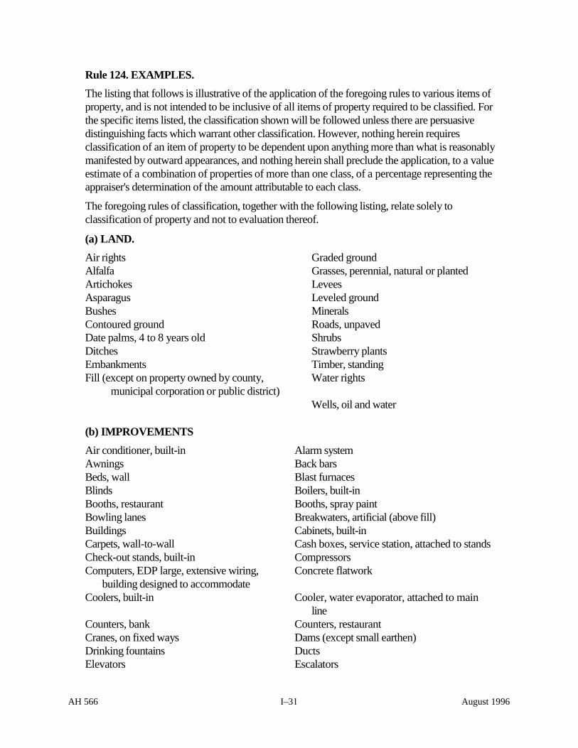
Rule 124. EXAMPLES. The listing that follows is illustrative of the application of the foregoing rules to various items of property, and is not intended to be inclusive of all items of property required to be classified. For the specific items listed, the classification shown will be followed unless there are persuasive distinguishing facts which warrant other classification. However, nothing herein requires classification of an item of property to be dependent upon anything more than what is reasonably manifested by outward appearances, and nothing herein shall preclude the application, to a value estimate of a combination of properties of more than one class, of a percentage representing the appraiser's determination of the amount attributable to each class.

The foregoing rules of classification, together with the following listing, relate solely to classification of property and not to evaluation thereof.

(a) LAND. Air rights Graded ground Alfalfa Grasses, perennial, natural or planted Artichokes Levees Asparagus Leveled ground Bushes Minerals Contoured ground Roads, unpaved Date palms, 4 to 8 years old Shrubs Ditches Strawberry plants Embankments Timber, standing Fill (except on property owned by county,

municipal corporation or public district) Water rights

Wells, oil and water

(b) IMPROVEMENTS Air conditioner, built-in Alarm system Awnings Back bars Beds, wall Blast furnaces Blinds Boilers, built-in Booths, restaurant Booths, spray paint Bowling lanes Breakwaters, artificial (above fill) Buildings Cabinets, built-in Carpets, wall-to-wall Cash boxes, service station, attached to stands Check-out stands, built-in Compressors Computers, EDP large, extensive wiring,

building designed to accommodate Concrete flatwork

Coolers, built-in Cooler, water evaporator, attached to main line

Counters, bank Counters, restaurant Cranes, on fixed ways Dams (except small earthen) Drinking fountains Ducts Elevators Escalators

AH 566 I–31 August 1996

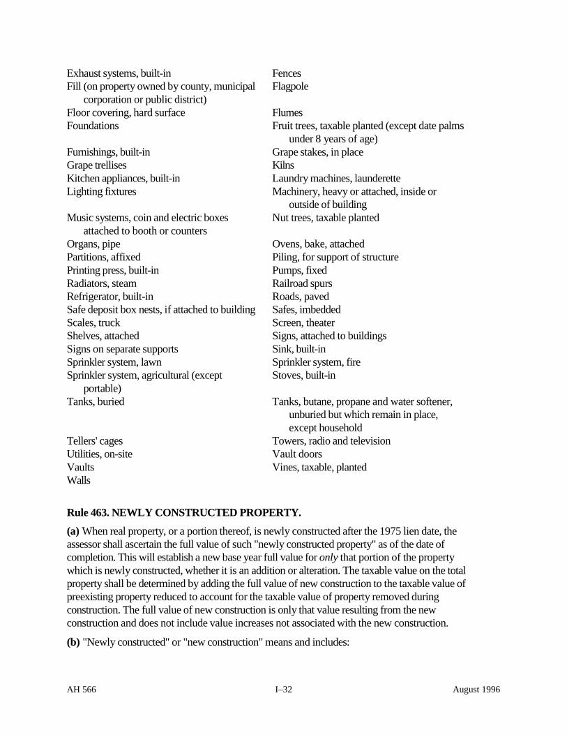
Exhaust systems, built-in Fences Fill (on property owned by county, municipal

corporation or public district) Flagpole

Floor covering, hard surface Flumes Foundations Fruit trees, taxable planted (except date palms

under 8 years of age) Furnishings, built-in Grape stakes, in place Grape trellises Kilns Kitchen appliances, built-in Laundry machines, launderette Lighting fixtures Machinery, heavy or attached, inside or

outside of building Music systems, coin and electric boxes

attached to booth or counters Nut trees, taxable planted

Organs, pipe Ovens, bake, attached Partitions, affixed Piling, for support of structure Printing press, built-in Pumps, fixed Radiators, steam Railroad spurs Refrigerator, built-in Roads, paved Safe deposit box nests, if attached to building Safes, imbedded Scales, truck Screen, theater Shelves, attached Signs, attached to buildings Signs on separate supports Sink, built-in Sprinkler system, lawn Sprinkler system, fire Sprinkler system, agricultural (except

portable) Stoves, built-in

Tanks, buried Tanks, butane, propane and water softener, unburied but which remain in place, except household

Tellers' cages Towers, radio and television Utilities, on-site Vault doors Vaults Vines, taxable, planted Walls

Rule 463. NEWLY CONSTRUCTED PROPERTY.

(a) When real property, or a portion thereof, is newly constructed after the 1975 lien date, the assessor shall ascertain the full value of such "newly constructed property" as of the date of completion. This will establish a new base year full value for only that portion of the property which is newly constructed, whether it is an addition or alteration. The taxable value on the total property shall be determined by adding the full value of new construction to the taxable value of preexisting property reduced to account for the taxable value of property removed during construction. The full value of new construction is only that value resulting from the new construction and does not include value increases not associated with the new construction.

(b) "Newly constructed" or "new construction" means and includes:

AH 566 I–32 August 1996

(1) Any substantial addition to land or improvements, including fixtures, such as adding land fill, retaining walls, curbs, gutters or sewers to land or constructing a new building or swimming pool or changing an existing improvement so as to add horizontally or vertically to its square footage or to incorporate an additional fixture, as that term is defined in this section.

(2) Any substantial physical alteration of land which constitutes a major rehabilitation of the land or results in a change in the way the property is used.

Examples of alterations to land to be considered new construction are:

Site development of rural land for the purpose of establishing a residential subdivision.

Altering rolling, dry grazing land to level irrigated crop land.

Preparing a vacant lot for use as a parking facility.

In any instance in which an alteration is substantial enough to require reappraisal, only the value of the alteration shall be added to the base year value of the pre-existing land or improvements. Increases in land value caused by appreciation or a zoning change rather than new construction shall not be enrolled, for example:

1. Land value 1975 = $10,000 2. Land value 1978 = $20,000 3. Value of alteration 1978 = $5,000 4. Value of structure

added 1978 = $75,000 1979 roll value (1+3+4) = $90,000 (must be adjusted to reflect appropriate

indexing) Alterations to land which do not constitute a major rehabilitation or which do not result in a change in the way the property is used shall not result in reappraisal.

(3) Any physical alteration of any improvement which converts the improvement or any portion thereof to the substantial equivalent of a new structure or portion thereof or changes the way in which the portion of the structure that had been altered is used, e.g., physical alterations to an old structure to make it the substantial equivalent of a new building without any change in the way it is used or alterations to a warehouse that makes it usable as a retail store or a restaurant. Only, the value, not necessarily the cost, of the alteration shall be added to the appropriately indexed base year value of the pre-existing structure.

(4) Excluded from alterations that qualify as "newly constructed" is construction or reconstruction performed for the purpose of normal maintenance and repair, e.g., routine annual preparation of agricultural land or interior or exterior painting, replacement of roof coverings or the addition of aluminum siding to improvements or the replacement of worn machine parts.

(5) Any substantial physical rehabilitation, renovation or modernization of any fixture which converts it to the substantial equivalent of a new fixture or any substitution of a new fixture.

Substantial equivalency shall be ascertained by comparing the productive capacity, normally expressed in units per hour, of the rehabilitated fixture to its original productive capacity.

AH 566 I–33 August 1996

(c) For purposes of this section, "fixture" is defined as an improvement whose use or purpose directly applies to or augments the process or function of a trade, industry, or profession.

(d) New construction in progress on the lien date shall be appraised at its full value on such date and each lien date thereafter until the date of completion, at which time the entire portion of property which is newly constructed shall be reappraised at its full value.

(e) For purposes of this section, the date of completion is the date the property or portion thereof is available for use. In determining whether the real property or a portion thereof is available for use, consideration shall be given to the date of the final inspection by the appropriate governmental official, or, in the absence of such inspection, the date the prime contractor fulfilled all of his contract obligations, or in the case of fixtures, the date of the completion of testing of machinery and equipment.

(f) Newly constructed property does not include real property which is timely reconstructed after a disaster where the full value of such real property, as reconstructed, is substantially equivalent to its full value prior to the disaster. If the values are not substantially equivalent, the assessor shall on lien date following restoration:

(1) Enroll the restored property at its former taxable value plus or minus the appropriate inflation adjustment, or

(2) Enroll the current market value of the restored property if the current market value is less than the value found in Item 1 above, or

(3) Enroll the value found in Item 1 above plus the market value of any newly constructed property if it is determined that new construction has occurred.

For purposes of this subsection only, newly constructed property does not include any land, improvement or fixture that is restored, reconstructed or repaired in a timely manner following a disaster and which is substantially equivalent in size, use and quality to that which existed prior to the disaster.

(g) For property under reconstruction or restoration as a result of disaster which changes ownership prior to the completion of reconstruction or restoration, the value of the land and existing improvements shall be determined as of the date of the change in ownership but the value of any reconstruction or restoration which occurs following the transfer shall be determined as of the date of completion in accordance with the provisions applicable to new construction but without regard to the "substantially equivalent" test normally applicable to property reconstructed following a disaster.

Rule 463.5. DATE OF COMPLETION OF NEW CONSTRUCTION -- SUPPLEMENTAL ASSESSMENTS

(a) APPLICATION. The provisions of this section are applicable only to supplemental assessments levied pursuant to Chapter 3.5 (commencing with Section 75) of Part 0.5 of Division 1 of the Revenue and Taxation Code.

(b) DATE OF COMPLETION OF NEW CONSTRUCTION. The date of completion of new construction resulting from actual physical new construction on the site shall be the earliest of

AH 566 I–34 August 1996

either the date upon which the new construction is available for use by the owner or, if all of the conditions of paragraph (b) (1) are satisfied, the date the property is occupied or used by the owner, or with the owner's consent, after the owner has provided a notice in accordance with paragraph (b) (1).

(1) The date of completion of new construction resulting from actual physical new construction shall not be the date upon which it is available for use if the owner does not intend to occupy or use the property and the owner notifies the assessor in writing prior to, or within 30 days after, the date of commencement of construction that he/she/it does not intend to occupy or use the identified property or a specified portion thereof.

(2) The date of completion of new construction resulting from actual physical new construction shall be conclusively presumed to be the date upon which the new construction is available for use by the owner if the assessor fails to receive notice as provided in paragraph (b) (1).

(c) DEFINITIONS. (1) "Property" means land, improvement(s) including fixtures, and mobilehome(s) subject to

taxation under Part 13 (commencing with Section 5800) of Division 1 of the Revenue and Taxation Code.

(2) "New Construction resulting from actual physical new construction" means "new construction" as defined in Section 463, subsections (b) and (f).

"New construction resulting from actual physical new construction" also includes: (A) the installation of a new fixture which is an addition or is a replacement of an existing fixture; (B) the rehabilitation, renovation or modernization of any fixture which converts it to the substantial equivalent of a new fixture; (C) the severance of improvements, including structures and fixtures, which is associated with new construction; (D) the severance on, or after, March 1, 1985, of fixtures which qualify for assessment pursuant to Sections 75.15 and 75.16 of the Revenue and Taxation Code, whether or not the severance is associated with other new construction; or (E) the severance on, or after, July 31, 1985, of structures, whether or not the severance is associated with other new construction.

"New construction resulting from actual physical new construction" does not include: (A) the severance prior to March 1, 1985, of improvements, including structures and fixtures, which is not associated with other new construction; (B) the severance on, or after, March 1, 1985 of any improvements, other than structures or fixtures, which is not associated with other new construction; (C) the severance prior to July 31, 1985, of structures which is not associated with other new construction; or (D) the discontinued use of improvements, including structures and fixtures, which are not physically severed from the property but which are made redundant by newly installed or erected structures, fixtures, or other improvements.

Examples:

(A) The installation of a multi-level printing press (a fixture) as an addition to existing facilities constitutes actual physical new construction.

(B) The installation of a printing press as the replacement of an existing press is also actual physical new construction.

AH 566 I–35 August 1996

(C) The complete renovation of an existing press to the substantial equivalent of a new press constitutes actual physical new construction.

(D) The severance of the old press (also a fixture) is actual physical new construction if it is associated with the installation of the new press or other new construction, or if it occurred on or after March 1, 1985.

(3) "Commencement of construction" means the performance of physical activities on the property which results in changes which are visible to any person inspecting the site and are recognizable as the initial steps for the preparation of land or the installation of improvements or fixtures. Such activities include clearing and grading land, layout of foundations, excavation of foundation footing, fencing the site, or installation of temporary structures. Such activities also include the severance of existing improvements or fixtures.

"Commencement of construction" does not include activities preparatory to actual construction such as obtaining architect services, preparing plans and specifications, obtaining building permits or zoning variances or filing subdivision maps or environmental impact reports.

"Commencement of construction" shall be determined solely on the basis of activities which occur and are apparent on the property undergoing new construction. Where several parcels are adjacent and will be used as a single unit by the builder for the construction project, the commencement of construction shall be determined on the basis of the activities which occur on any part of the several parcels comprising the unit. Where a property has been subdivided into separate lots, the commencement of construction shall be determined on the basis of the activities occurring on each separate lot. Where the property has been subdivided into separate lots and several or all of those lots will be used as a single unit by the builder for the construction project, the commencement of construction shall be determined on the basis of the activities which occur on any part of the several parcels comprising the unit.

(4) "Available for use" means that the property, or a portion thereof, has been inspected and approved for occupancy by the appropriate governmental official or, in the absence of such inspection and approval procedures, when the prime contractor has fulfilled all of the contractual obligations. When inspection and approval procedures are non-existent or exist but are not utilized and a prime contractor is not involved, the newly constructed property is available for use when outward appearances clearly indicate it is immediately usable for the purpose intended. Fixtures are available for use when all testing necessary for proper operation or safety is completed.

New construction is not available for use if, on the date it is otherwise available for use, it cannot be functionally used or occupied. In that case, the property is not available for use until the date that any legal or physical impediment to functional use or occupancy is removed.

If a structure is constructed with the expectation that the tenant(s) will have improvements added after a lease(s) is executed, "available for use" means that point in time when the structure is ready to receive tenant improvements, whether or not there are any tenants at that time and regardless of who is to construct the improvements. If a construction project is completed in stages with some portions available for occupancy prior to completion of the total project, any portion of the project ready to receive tenant improvements is available for use even though other portions of the project are not ready for such improvements. In the case of physical alterations to land, such as leveling, "available for use" means that point in time when the land is ready for use by the owner and no

AH 566 I–36 August 1996

further new construction is required for the new use. In the case of fixtures added as part of a larger new construction project, "available for use" means that point in time when the project, including the fixture, is ready for use.

(5) "Occupied or used" means the physical occupancy of the property by the owner or any physical use of the property by the owner, except where such occupancy or use is incidental to an offer for a change of ownership. "Occupied or used" also includes the rental or lease of the property or any occupancy or use of the property by third persons with the owner's consent. The occupancy or use of the property occurs on the earliest date when the property is physically occupied or used, or when the agreed upon term of occupancy commences. "Used" does not include the transfer of legal title to the property as security.

(6) "Functionally used or occupied" means that the property is or can be used or occupied for the purpose for which it was constructed. The purpose for which the property was constructed or improved shall be determined on the basis of the type of property and any special facts or circumstances which affect its use or occupancy. Property shall not be considered "functionally used or occupied" if any legal restriction or physical impediment beyond the owners' control prevents the use of the property for the purpose intended.

Examples:

(A) A building intended for use as a warehouse can be functionally used when physical construction is completed even though the property to be stored has not arrived at the site.

(B) Land improved by leveling and the installation of an irrigation system which converts it from grazing land to farm land can be functionally used when the improvement activity is completed even though the planting season will not commence for several months.

(C) An office or hotel building on which construction is completed cannot be functionally used if it is uninhabitable because of the lack of power, water or sewer service, or if a natural disaster, such as a flood or earth slide, prevents reasonable public access to the facility.

(7) "Owner's consent" means the express or implied agreement of an owner to allow the property, or a portion thereof, to be physically occupied or used by a third person. Where the use or occupancy is visible to, or ascertainable by, the assessor, it shall be rebuttably presumed that the property is occupied or used with the owner's consent. If the owner has received actual or constructive notice of the occupancy or use, failure of the owner to communicate an objection to the user or enforce his rights to remove the occupant within a reasonable time shall be evidence of consent.

(8) "Incidental to an offer for a change of ownership" means that an activity is usual or necessary to the holding of property for sale in the regular course of business. It includes any use or occupancy arising from the demonstration or display of the property for the purpose of selling that property or other property in the vicinity under the same ownership. It includes use of the property by the owner or by any person using the property with the owner's consent. Use of property as a model home, a sales office, or as a temporary storage facility for building materials or furnishings intended to be installed in other property to be held for sale, shall be considered to be incidental to an offer for a change in ownership. Temporary use of the property as lodging by a potential buyer for the purpose of sales promotion shall be considered incidental to an offer for a change of

AH 566 I–37 August 1996

ownership. The use of this property, however, by a potential buyer as a principal residence pending the arrangement or approval of the financing necessary to complete the purchase is not incidental to an offer for a change in ownership.

(9) "Structures" means all improvements subject to supplemental assessment other than living improvements (trees and vines) and fixtures which qualify for assessment pursuant to Sections 75.15 and 75.16 of the Revenue and Taxation Code.

Rule 468. OIL AND GAS PRODUCING PROPERTIES.

(a) The right to remove petroleum and natural gas from the earth is a taxable real property interest. Increases in recoverable amounts of such minerals caused by changed physical or economic conditions constitute additions to such a property interest. Reduction in recoverable amounts of minerals caused by production or changes in the expectation of future production capabilities constitute a reduction in the interest. Whether or not physical changes to the system employed in recovering such minerals qualify as new construction shall be determined by reference to Section 463(a).

(b) The market value of an oil and gas mineral property interest is determined by estimating the value of the volumes of proved reserves. Proved reserves are those reserves which geological and engineering information indicate with reasonable certainty to be recoverable in the future, taking into account reasonably projected physical and economic operating conditions. Present and projected economic conditions shall be determined by reference to all economic factors considered by knowledgeable and informed persons engaged in the operation and buying or selling of such properties, e.g., capitalization rates, product prices and operation expenses.

(c) The unique nature of oil and gas property interests requires the application of specialized appraisal techniques designed to satisfy the requirements of Article XIII, Section 1, and Article XIII A, Section 2, of the California Constitution. To this end, the valuation of such properties and other real property associated therewith shall be pursuant to the following principles and procedures:

(1) A base year value (market value) of the property shall be estimated as of lien date 1975 in accordance with Section 460.1 or as of the date a change in ownership occurs subsequent to lien date 1975. Newly constructed improvements and additions in reserves shall be valued as of the lien date of the year for which the roll is being prepared. Improvements removed from the site shall be deducted from taxable value. Base year values shall be determined using factual market data such as prices and expenses ordinarily considered by knowledgeable and informed persons engaged in the operation, buying and selling of oil, gas and other mineral-producing properties and the production therefrom. Once determined, a base year value may be increased no more than two percent per year.

(2) Base year reserve values must be adjusted annually for the value of depleted reserves caused by production or changes in the expectation of future production.

(3) Additions to reserves established in a given year by discovery, construction of improvements, or changes in economic conditions shall be quantified and appraised at market value.

AH 566 I–38 August 1996

(4) The current year's lien date taxable value of mineral reserves shall be calculated as follows:

(A) The total unit market value and the volume of reserves using current market data shall be estimated.

(B) The current value of taxable reserves is determined by segregating the value of wells, casings, and parts thereof, land (other than mineral rights) and improvements from the property unit value by an allocation based on the value of such properties.

(C) The volume of new reserves shall be determined by subtracting the prior year's reserves, less depletions, from the estimated current total reserves.

(D) The value of removed reserves shall be calculated by multiplying the volume of the reserves removed in the prior year by the weighted average value, for reserves only, per unit of minerals for all prior base years. The prior year's taxable value of the reserves remaining from prior years shall be found by subtracting the value of removed reserves from the prior year's taxable value.

(E) The new reserves are valued by multiplying the new volume by the current market value per unit of the total reserves.

(F) The current taxable value for reserves only is the sum of the value of the prior year's reserves, net of depletions as calculated in (D) above, factored by the appropriate percentage change in the Consumer Price Index (CPI) added to the value of the new reserves, as calculated in (E) above.

(5) Valuation of land (other than mineral reserves) and improvements.

(A) A base year value (market value) of land (including wells, casings and parts thereof) and improvements shall be estimated as of lien date 1975 in accordance with Section 460.1, the date of new construction after 1975, or the date a change of ownership occurs subsequent to lien date 1975.

(B) The value of land (wells, casings and parts thereof) and improvements shall remain at their factored base year value except as provided in (6) below.

(6) Value declines shall be recognized when the market value of the appraisal unit, i.e., land, improvements and reserves, is less than the current taxable value of the same unit.

AH 566 I–39 August 1996

BIBLIOGRAPHY

Allen, Fraser H. and Seba, Richard D., Economics of Worldwide Petroleum Production, Oil & Gas Consultants International, Inc., Tulsa, Oklahoma, 1993

Annual Report of the State Oil & Gas Supervisor, California Department of Conservation, Division of Oil, Gas, & Geothermal Resources

California Department of Conservation, Division of Oil and Gas (Personal communication with Sue Hodgeson)

Campbell, John M., Jr., Campbell, John M., Sr. and Campbell Robert A., Analysis and Management of Petroleum Investments: Risk Taxes and Time, CPS, Norman, Oklahoma, 1987

Encyclopedia Britannica, 1995, Compact Disc Version

Gray, Forest, Petroleum Production for the Non-Technical Person, Pennwell Publishing, Tulsa, Oklahoma, (1986)

Guidelines For Application of the Definitions for Oil and Gas Reserves, Society of Petroleum Evaluation Engineers, Dallas, Tx., (1988)

Petroleum Engineering Handbook, Howard B. Bradley (ed.), Society of Petroleum Engineers, Richardson, TX, 1987

Petroleum Engineering, 1976, Alfred Mayer-Gürr, Halsted Press

Petroleum Production Handbook, Society of Petroleum Engineers, 1962

Petroleum, Mineral Commodities of California, Bulletin 176, Division of Mines, Department of Natural Resources, 1957

Preliminary Report of Oil and Gas Production Statistics, Department of Conservation, Division of Oil, Gas, and Geothermal Resources

Primer of Oil and Gas Production, American Petroleum Institute, Dallas, Tx., (1976)

Thompson, Robert S. and Wright, John D., Oil Property Evaluation, Thompsom-Wright Associates, Golden, Colorado, 1985

Timmerman, E.H., Practical Reservoir Engineering, PennWell Publishing Company, Tulsa, Oklahoma, 1982

van Poollen, H.K. and Associates Inc., Fundamentals of Enhanced Oil Recovery, PennWell Publishing Company, Tulsa, Oklahoma, 1980

Willhite, G. Paul, Waterflooding, Society of Petroleum Engineers, Richardson, TX (1986)

Williamson, Harold F. and Daum, Arnold R., The American Petroleum Industry: The Age Of Illumination 1859-1899, Northwestern University Press, Evanston, 1959

AH 566 August 1996

World Oil, 1978, Selecting Enhanced Oil Recovery Processes, Aniekan Willie Iyoho

Yergin, Daniel, The Prize: The Epic Quest for Oil Money & Power, Simon & Schuster, New York, 1992

AH 566 August 1996