Embed Size (px)
Citation preview

SSD: Single Shot MultiBox Detector
Presented by Hongyan Wang and Nathan Watts
Wei Liu(1), Dragomir Anguelov(2), Dumitru Erhan(3), Christian Szegedy(3), Scott Reed(4), Cheng-Yang Fu(1), Alexander C. Berg(1)
UNC Chapel Hill(1), Zoox Inc.(2), Google Inc.(3), University of Michigan(4)
Original slides are from http://www.cs.unc.edu/~wliu/papers/ssd_eccv2016_slide.pdf
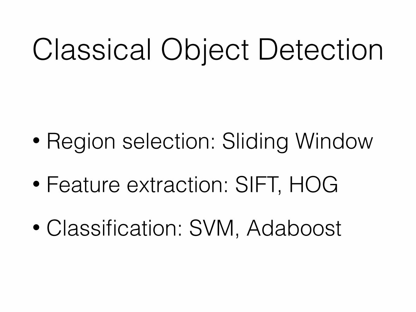
Classical Object Detection
• Region selection: Sliding Window
• Feature extraction: SIFT, HOG
• Classification: SVM, Adaboost
Original slides are from http://cs231n.stanford.edu/slides/winter1516_lecture8.pdf

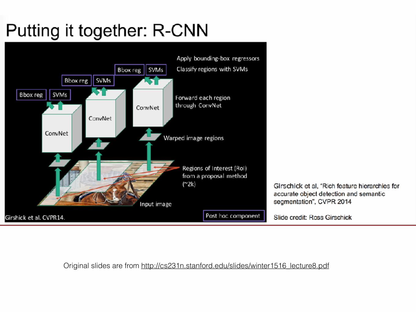
R-CNN problems• Slow at test time: need to run full forward pass of
CNN for each region proposal.
• Complex training pipeline
Original slides are from http://cs231n.stanford.edu/slides/winter1516_lecture8.pdf

Original slides are from http://cs231n.stanford.edu/slides/winter1516_lecture8.pdf

Fast R-CNN problem
• Region proposal is the bottleneck.
Original slides are from http://cs231n.stanford.edu/slides/winter1516_lecture8.pdf

Original slides are from http://cs231n.stanford.edu/slides/winter1516_lecture8.pdf

Original slides are from http://cs231n.stanford.edu/slides/winter1516_lecture8.pdf

Faster R-CNN problem
• Still slow for real-time detection.
Original slides are from http://cs231n.stanford.edu/slides/winter1516_lecture8.pdf

Original slides are from http://cs231n.stanford.edu/slides/winter1516_lecture8.pdf
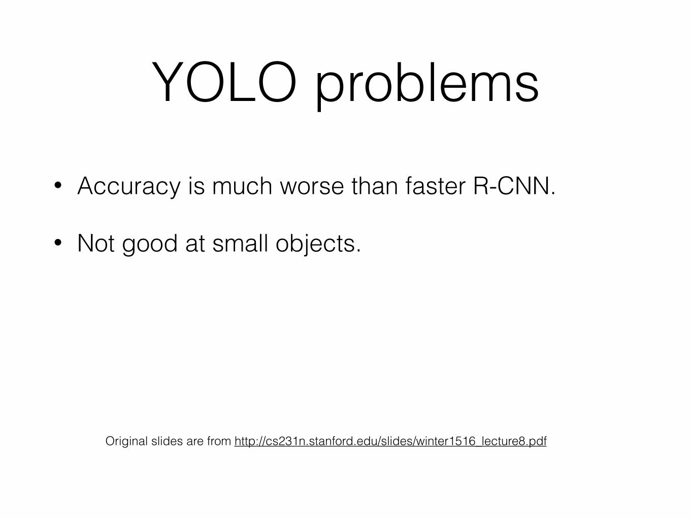
YOLO problems• Accuracy is much worse than faster R-CNN.
• Not good at small objects.
Original slides are from http://cs231n.stanford.edu/slides/winter1516_lecture8.pdf

Next ? SSD !

VGGNet Titan X Pascal
Original slides are from http://www.cs.unc.edu/~wliu/papers/ssd_eccv2016_slide.pdf

VGGNet Titan X Pascal
Original slides are from http://www.cs.unc.edu/~wliu/papers/ssd_eccv2016_slide.pdf

10 20 30 40 50Speed (fps)
70
80VO
C20
07 te
st m
AP
R-CNN, Girshick 201466% mAP / 0.02 fps
Fast R-CNN, Girshick 201570% mAP / 0.4 fps
Faster R-CNN, Ren 201573% mAP / 7 fps
YOLO, Redmon 201666% mAP / 21 fps
All with VGGNet pretrained on ImageNet, batch_size = 1 on Titan X
Original slides are from http://www.cs.unc.edu/~wliu/papers/ssd_eccv2016_slide.pdf

10 20 30 40 50Speed (fps)
70
80VO
C20
07 te
st m
AP
R-CNN, Girshick 201466% mAP / 0.02 fps
Fast R-CNN, Girshick 201570% mAP / 0.4 fps
Faster R-CNN, Ren 201573% mAP / 7 fps
YOLO, Redmon 201666% mAP / 21 fps
10 20 30 40 50Speed (fps)
70
80VO
C20
07 te
st m
AP
R-CNN, Girshick 201466% mAP / 0.02 fps
Fast R-CNN, Girshick 201570% mAP / 0.4 fps
Faster R-CNN, Ren 201573% mAP / 7 fps
YOLO, Redmon 201666% mAP / 21 fps
SSD30074% mAP / 46 fps
6.6x faster
10 20 30 40 50Speed (fps)
70
80VO
C20
07 te
st m
AP
R-CNN, Girshick 201466% mAP / 0.02 fps
Fast R-CNN, Girshick 201570% mAP / 0.4 fps
Faster R-CNN, Ren 201573% mAP / 7 fps
YOLO, Redmon 201666% mAP / 21 fps
SSD30074% mAP / 46 fps
SSD51277% mAP / 19 fps
11% better
10 20 30 40 50Speed (fps)
70
80VO
C20
07 te
st m
AP
R-CNN, Girshick 201466% mAP / 0.02 fps
Fast R-CNN, Girshick 201570% mAP / 0.4 fps
Faster R-CNN, Ren 201573% mAP / 7 fps SSD300
74% mAP / 46 fps
YOLO, Redmon 201666% mAP / 21 fps
SSD51277% mAP / 19 fps
SSD30077% mAP / 46 fps
SSD51280% mAP / 19 fps
All with VGGNet pretrained on ImageNet, batch_size = 1 on Titan X
Original slides are from http://www.cs.unc.edu/~wliu/papers/ssd_eccv2016_slide.pdf

10 20 30 40 50Speed (fps)
70
80VO
C20
07 te
st m
AP
R-CNN, Girshick 201466% mAP / 0.02 fps
Fast R-CNN, Girshick 201570% mAP / 0.4 fps
Faster R-CNN, Ren 201573% mAP / 7 fps
YOLO, Redmon 201666% mAP / 21 fps
SSD30077% mAP / 46 fps
SSD51280% mAP / 19 fps
Two-Stage
box proposal + postclassify Single Shot
Original slides are from http://www.cs.unc.edu/~wliu/papers/ssd_eccv2016_slide.pdf

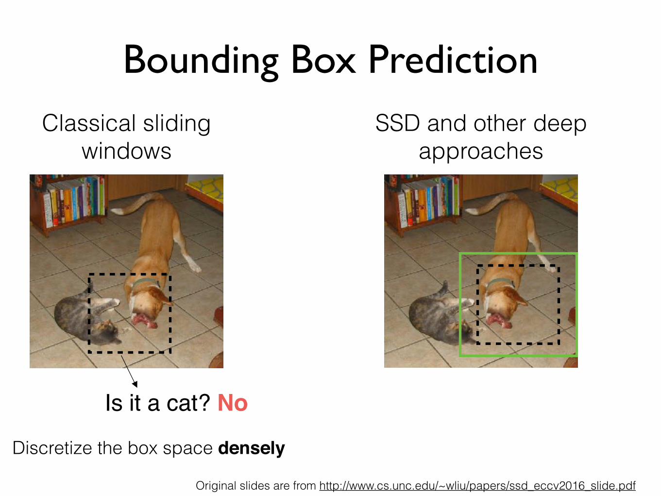
Classical sliding windows
Bounding Box Prediction
Original slides are from http://www.cs.unc.edu/~wliu/papers/ssd_eccv2016_slide.pdf

Classical sliding windows
Bounding Box Prediction
Is it a cat? No
Original slides are from http://www.cs.unc.edu/~wliu/papers/ssd_eccv2016_slide.pdf

Is it a cat? No
Discretize the box space densely
Classical sliding windows
Bounding Box Prediction
Original slides are from http://www.cs.unc.edu/~wliu/papers/ssd_eccv2016_slide.pdf

SSD and other deep approaches
Is it a cat? No
Discretize the box space densely
Classical sliding windows
Bounding Box Prediction
Original slides are from http://www.cs.unc.edu/~wliu/papers/ssd_eccv2016_slide.pdf

SSD and other deep approaches
Is it a cat? No
Discretize the box space densely
Classical sliding windows
Bounding Box Prediction
Original slides are from http://www.cs.unc.edu/~wliu/papers/ssd_eccv2016_slide.pdf

SSD and other deep approaches
cat: 0.8 dog: 0.1Is it a cat? No
Discretize the box space densely
Classical sliding windows
Bounding Box Prediction
Original slides are from http://www.cs.unc.edu/~wliu/papers/ssd_eccv2016_slide.pdf

SSD and other deep approaches
Is it a cat? No
Classical sliding windows
Bounding Box Prediction
Discretize the box space densely
Original slides are from http://www.cs.unc.edu/~wliu/papers/ssd_eccv2016_slide.pdf
SSD and other deep approaches
Is it a cat? No
Classical sliding windows
Bounding Box Prediction
Discretize the box space densely
Original slides are from http://www.cs.unc.edu/~wliu/papers/ssd_eccv2016_slide.pdf

SSD and other deep approaches
Is it a cat? No
Classical sliding windows
Bounding Box Prediction
Discretize the box space densely
Original slides are from http://www.cs.unc.edu/~wliu/papers/ssd_eccv2016_slide.pdf

SSD and other deep approaches
dog: 0.4 cat: 0.2Is it a cat? No
Classical sliding windows
Bounding Box Prediction
Discretize the box space densely
Original slides are from http://www.cs.unc.edu/~wliu/papers/ssd_eccv2016_slide.pdf

SSD and other deep approaches
dog: 0.4 cat: 0.2Is it a cat? No
Classical sliding windows
Bounding Box Prediction
Discretize the box space more coarselyRefine the coordinates of each boxDiscretize the box space densely
Original slides are from http://www.cs.unc.edu/~wliu/papers/ssd_eccv2016_slide.pdf

ConvNet
feature map
SSD Output Layer
Original slides are from http://www.cs.unc.edu/~wliu/papers/ssd_eccv2016_slide.pdf

ConvNet
feature map
SSD Output Layer
small (e.g. 3x3) conv kernel
Original slides are from http://www.cs.unc.edu/~wliu/papers/ssd_eccv2016_slide.pdf

ConvNet
feature map
SSD Output Layer
small (e.g. 3x3) conv kernel
default box
Original slides are from http://www.cs.unc.edu/~wliu/papers/ssd_eccv2016_slide.pdf

feature map
box regression
multiclass probabilities
SSD Output Layer
ConvNet
Original slides are from http://www.cs.unc.edu/~wliu/papers/ssd_eccv2016_slide.pdf

ConvNet
feature map
box regression
multiclass probabilities
SSD Training• Match default boxes to ground truth boxes to determine true/false positives.
• Loss = SmoothL1(box param) + Softmax(class prob)
Smooth L1 loss Softmax loss
Original slides are from http://www.cs.unc.edu/~wliu/papers/ssd_eccv2016_slide.pdf

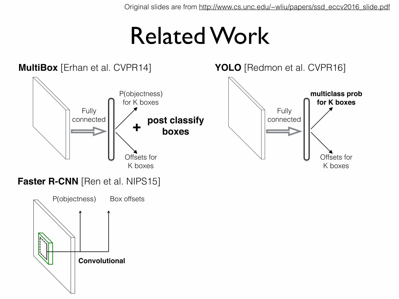
Related WorkOriginal slides are from http://www.cs.unc.edu/~wliu/papers/ssd_eccv2016_slide.pdf

Related WorkMultiBox [Erhan et al. CVPR14]
P(objectness) for K boxes
Fully connected
Offsets for K boxes
Original slides are from http://www.cs.unc.edu/~wliu/papers/ssd_eccv2016_slide.pdf

Related WorkMultiBox [Erhan et al. CVPR14]
P(objectness) for K boxes
Fully connected
Offsets for K boxes
+ post classify boxes
Original slides are from http://www.cs.unc.edu/~wliu/papers/ssd_eccv2016_slide.pdf

Related WorkYOLO [Redmon et al. CVPR16]
multiclass probfor K boxes
Fully connected
Offsets for K boxes
MultiBox [Erhan et al. CVPR14]
P(objectness) for K boxes
Fully connected
Offsets for K boxes
+ post classify boxes
Original slides are from http://www.cs.unc.edu/~wliu/papers/ssd_eccv2016_slide.pdf
Related WorkYOLO [Redmon et al. CVPR16]
multiclass probfor K boxes
Fully connected
Offsets for K boxes
Faster R-CNN [Ren et al. NIPS15]
Convolutional
P(objectness) Box offsets
MultiBox [Erhan et al. CVPR14]
P(objectness) for K boxes
Fully connected
Offsets for K boxes
+ post classify boxes
Original slides are from http://www.cs.unc.edu/~wliu/papers/ssd_eccv2016_slide.pdf

Related WorkYOLO [Redmon et al. CVPR16]
multiclass probfor K boxes
Fully connected
Offsets for K boxes
Faster R-CNN [Ren et al. NIPS15]
Convolutional
P(objectness) Box offsets
+ post classify boxes
MultiBox [Erhan et al. CVPR14]
P(objectness) for K boxes
Fully connected
Offsets for K boxes
+ post classify boxes
Original slides are from http://www.cs.unc.edu/~wliu/papers/ssd_eccv2016_slide.pdf

Related WorkYOLO [Redmon et al. CVPR16]
multiclass probfor K boxes
Fully connected
Offsets for K boxes
Faster R-CNN [Ren et al. NIPS15]
Convolutional
P(objectness) Box offsets
SSD
Convolutional
Box offsetsmulticlass prob
+ post classify boxes
MultiBox [Erhan et al. CVPR14]
P(objectness) for K boxes
Fully connected
Offsets for K boxes
+ post classify boxes
Original slides are from http://www.cs.unc.edu/~wliu/papers/ssd_eccv2016_slide.pdf

Contribution #1:Multi-Scale Feature Maps
ConvNet
box regression
multiclass scores
Original slides are from http://www.cs.unc.edu/~wliu/papers/ssd_eccv2016_slide.pdf

Contribution #1:Multi-Scale Feature Maps
ConvNet
box regression
multiclass scores
stride 2 convolution
Original slides are from http://www.cs.unc.edu/~wliu/papers/ssd_eccv2016_slide.pdf

Contribution #1:Multi-Scale Feature Maps
ConvNet
box regression
multiclass scores
box regression
multiclass scores
stride 2 convolution
Original slides are from http://www.cs.unc.edu/~wliu/papers/ssd_eccv2016_slide.pdf

8⇥ 8 feature map 4⇥ 4 feature map
vs.
8⇥ 8 feature map
SSD
Multi-Scale Feature Maps
Original slides are from http://www.cs.unc.edu/~wliu/papers/ssd_eccv2016_slide.pdf

8⇥ 8 feature map 4⇥ 4 feature map
vs.
8⇥ 8 feature map
SSD
Multi-Scale Feature Maps
Faster R-CNN Objectness Proposal, Ren 2015
Original slides are from http://www.cs.unc.edu/~wliu/papers/ssd_eccv2016_slide.pdf

Prediction source layers from:
mAP
use boundary boxes?
# Boxes
38⇥ 38 19⇥ 19 10⇥ 10 5⇥ 5 3⇥ 3 1⇥ 1 Yes No
4 4 4 4 4 4 74.3 63.4 8732
4 4 4 70.7 69.2 9864
4 62.4 64.0 8664
Multi-Scale Feature Maps Experiment
Original slides are from http://www.cs.unc.edu/~wliu/papers/ssd_eccv2016_slide.pdf

Prediction source layers from:
mAP
use boundary boxes?
# Boxes
38⇥ 38 19⇥ 19 10⇥ 10 5⇥ 5 3⇥ 3 1⇥ 1 Yes No
4 4 4 4 4 4 74.3 63.4 8732
4 4 4 70.7 69.2 9864
4 62.4 64.0 8664
Multi-Scale Feature Maps Experiment
Original slides are from http://www.cs.unc.edu/~wliu/papers/ssd_eccv2016_slide.pdf

Prediction source layers from:
mAP
use boundary boxes?
# Boxes
38⇥ 38 19⇥ 19 10⇥ 10 5⇥ 5 3⇥ 3 1⇥ 1 Yes No
4 4 4 4 4 4 74.3 63.4 8732
4 4 4 70.7 69.2 9864
4 62.4 64.0 8664
Multi-Scale Feature Maps Experiment
Original slides are from http://www.cs.unc.edu/~wliu/papers/ssd_eccv2016_slide.pdf

Prediction source layers from:
mAP
use boundary boxes?
# Boxes
38⇥ 38 19⇥ 19 10⇥ 10 5⇥ 5 3⇥ 3 1⇥ 1 Yes No
4 4 4 4 4 4 74.3 63.4 8732
4 4 4 70.7 69.2 9864
4 62.4 64.0 8664
Multi-Scale Feature Maps Experiment
Original slides are from http://www.cs.unc.edu/~wliu/papers/ssd_eccv2016_slide.pdf

Prediction source layers from:
mAP
use boundary boxes?
# Boxes
38⇥ 38 19⇥ 19 10⇥ 10 5⇥ 5 3⇥ 3 1⇥ 1 Yes No
4 4 4 4 4 4 74.3 63.4 8732
4 4 4 70.7 69.2 9864
4 62.4 64.0 8664
Multi-Scale Feature Maps Experiment
Original slides are from http://www.cs.unc.edu/~wliu/papers/ssd_eccv2016_slide.pdf

Prediction source layers from:
mAP
use boundary boxes?
# Boxes
38⇥ 38 19⇥ 19 10⇥ 10 5⇥ 5 3⇥ 3 1⇥ 1 Yes No
4 4 4 4 4 4 74.3 63.4 8732
4 4 4 70.7 69.2 9864
4 62.4 64.0 8664
Multi-Scale Feature Maps Experiment
Original slides are from http://www.cs.unc.edu/~wliu/papers/ssd_eccv2016_slide.pdf

boundary boxes
Prediction source layers from:
mAP
use boundary boxes?
# Boxes
38⇥ 38 19⇥ 19 10⇥ 10 5⇥ 5 3⇥ 3 1⇥ 1 Yes No
4 4 4 4 4 4 74.3 63.4 8732
4 4 4 70.7 69.2 9864
4 62.4 64.0 8664
Multi-Scale Feature Maps Experiment
Original slides are from http://www.cs.unc.edu/~wliu/papers/ssd_eccv2016_slide.pdf

Prediction source layers from:
mAP
use boundary boxes?
# Boxes
38⇥ 38 19⇥ 19 10⇥ 10 5⇥ 5 3⇥ 3 1⇥ 1 Yes No
4 4 4 4 4 4 74.3 63.4 8732
4 4 4 70.7 69.2 9864
4 62.4 64.0 8664
Multi-Scale Feature Maps Experiment
Original slides are from http://www.cs.unc.edu/~wliu/papers/ssd_eccv2016_slide.pdf

Prediction source layers from:
mAP
use boundary boxes?
# Boxes
38⇥ 38 19⇥ 19 10⇥ 10 5⇥ 5 3⇥ 3 1⇥ 1 Yes No
4 4 4 4 4 4 74.3 63.4 8732
4 4 4 70.7 69.2 9864
4 62.4 64.0 8664
Multi-Scale Feature Maps Experiment
Original slides are from http://www.cs.unc.edu/~wliu/papers/ssd_eccv2016_slide.pdf

Contribution #2:Splitting the Region Space
ConvNet convolution
Original slides are from http://www.cs.unc.edu/~wliu/papers/ssd_eccv2016_slide.pdf

SSD300include { 1
2 , 2} box? 4 4include { 1
3 , 3} box? 4number of Boxes 3880 7760 8732
VOC2007 test mAP 71.6 73.7 74.3
Contribution #2:Splitting the Region Space
ConvNet convolution
Original slides are from http://www.cs.unc.edu/~wliu/papers/ssd_eccv2016_slide.pdf

Contribution #2:Splitting the Region Space
ConvNet convolution
Use 38x38 feature map : +2.5 mAP (conv4_3)
Original slides are from http://www.cs.unc.edu/~wliu/papers/ssd_eccv2016_slide.pdf

Why So Many Default Boxes?Faster R-CNN YOLO SSD300 SSD512
# Default Boxes 6000 98 8732 24564Resolution 1000x600 448x448 300x300 512x512
Original slides are from http://www.cs.unc.edu/~wliu/papers/ssd_eccv2016_slide.pdf

Why So Many Default Boxes?Faster R-CNN YOLO SSD300 SSD512
# Default Boxes 6000 98 8732 24564Resolution 1000x600 448x448 300x300 512x512
Original slides are from http://www.cs.unc.edu/~wliu/papers/ssd_eccv2016_slide.pdf

Why So Many Default Boxes?Faster R-CNN YOLO SSD300 SSD512
# Default Boxes 6000 98 8732 24564Resolution 1000x600 448x448 300x300 512x512
GT
Original slides are from http://www.cs.unc.edu/~wliu/papers/ssd_eccv2016_slide.pdf

Why So Many Default Boxes?Faster R-CNN YOLO SSD300 SSD512
# Default Boxes 6000 98 8732 24564Resolution 1000x600 448x448 300x300 512x512
GT DETECTION
Original slides are from http://www.cs.unc.edu/~wliu/papers/ssd_eccv2016_slide.pdf

Why So Many Default Boxes?Faster R-CNN YOLO SSD300 SSD512
# Default Boxes 6000 98 8732 24564Resolution 1000x600 448x448 300x300 512x512
• SmoothL1 or L2 loss for box shape averages among likely hypotheses
• Need to have enough default boxes (discrete bins) to do accurate regression in each
• General principle for regressing complex continuous outputs with deep nets
GT DETECTION
Original slides are from http://www.cs.unc.edu/~wliu/papers/ssd_eccv2016_slide.pdf

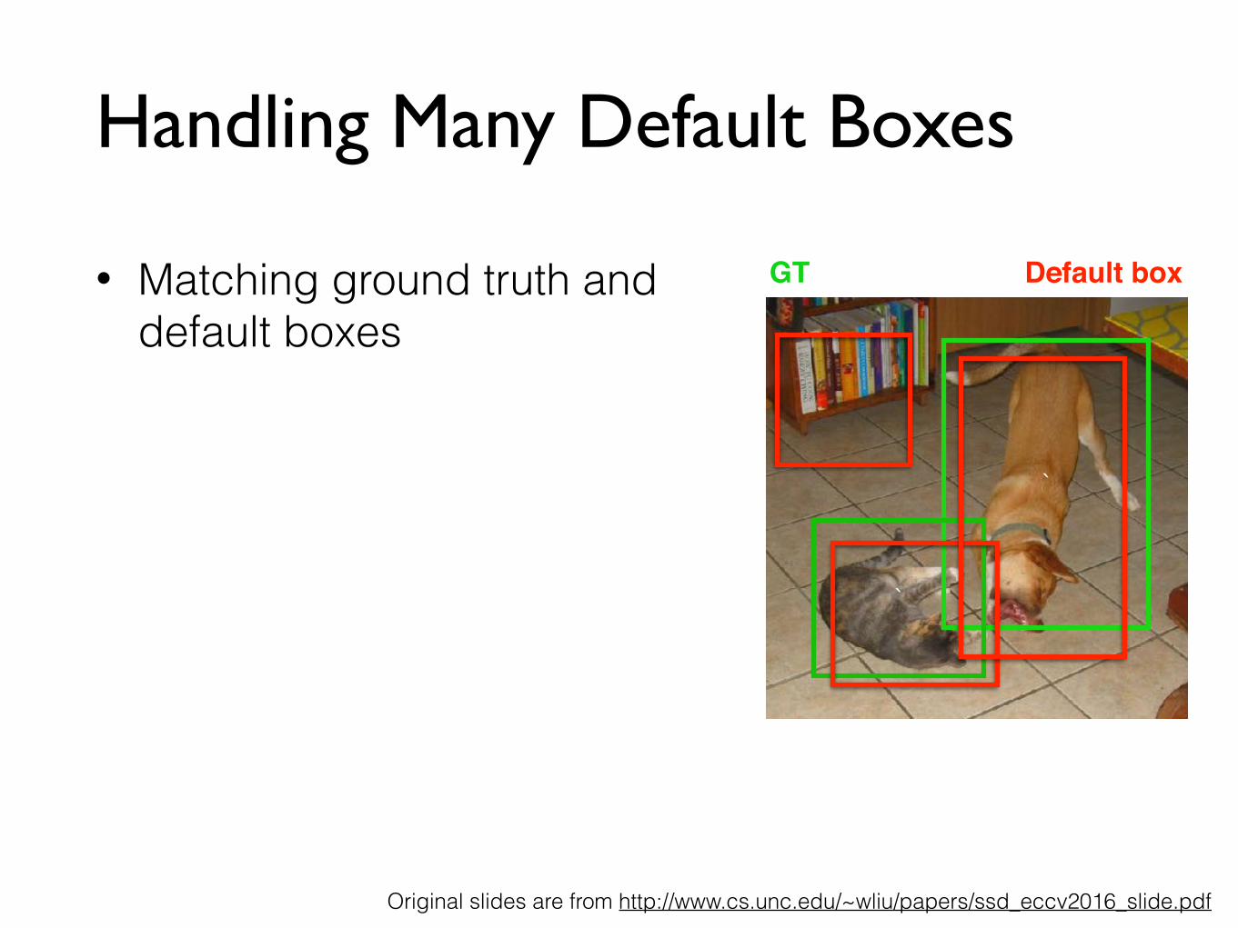
Handling Many Default Boxes
Original slides are from http://www.cs.unc.edu/~wliu/papers/ssd_eccv2016_slide.pdf

• Matching ground truth and default boxes
Handling Many Default Boxes
Original slides are from http://www.cs.unc.edu/~wliu/papers/ssd_eccv2016_slide.pdf

• Matching ground truth and default boxes
Handling Many Default Boxes
`
`
GT
Original slides are from http://www.cs.unc.edu/~wliu/papers/ssd_eccv2016_slide.pdf
• Matching ground truth and default boxes
Handling Many Default Boxes
`
`
GT Default box
Original slides are from http://www.cs.unc.edu/~wliu/papers/ssd_eccv2016_slide.pdf

• Matching ground truth and default boxes
Handling Many Default Boxes
`
`
GT Default box
TP
TP
FP
Original slides are from http://www.cs.unc.edu/~wliu/papers/ssd_eccv2016_slide.pdf

• Matching ground truth and default boxes
Handling Many Default Boxes
`
`
GT Default box
TP
TP
FP
?
Original slides are from http://www.cs.unc.edu/~wliu/papers/ssd_eccv2016_slide.pdf

• Matching ground truth and default boxes‣ Match each GT box to closest default box
Handling Many Default Boxes
`
`
GT Default box
TP
TP
FP
?
Original slides are from http://www.cs.unc.edu/~wliu/papers/ssd_eccv2016_slide.pdf

• Matching ground truth and default boxes‣ Match each GT box to closest default box
‣ Also match each GT box to all unassigned default boxes with IoU > 0.5
Handling Many Default Boxes
`
`
GT Default box
TP
TP
FP
?
Original slides are from http://www.cs.unc.edu/~wliu/papers/ssd_eccv2016_slide.pdf

• Matching ground truth and default boxes‣ Match each GT box to closest default box
‣ Also match each GT box to all unassigned default boxes with IoU > 0.5
• Hard negative mining
Handling Many Default Boxes
`
`
GT Default box
TP
TP
FP
?
Original slides are from http://www.cs.unc.edu/~wliu/papers/ssd_eccv2016_slide.pdf

• Matching ground truth and default boxes‣ Match each GT box to closest default box
‣ Also match each GT box to all unassigned default boxes with IoU > 0.5
• Hard negative mining• Unbalanced training: 1-30 TP, 8k-25k FP
• Keep TP:FP ratio fixed (1:3), use worst-misclassified FPs.
Handling Many Default Boxes
`
`
GT Default box
TP
TP
FP
?
Original slides are from http://www.cs.unc.edu/~wliu/papers/ssd_eccv2016_slide.pdf

SSD Architecture
300
VGG16
Det
ectio
ns:8
732
per
Cla
ss
Classifier : Conv: 3x3x(3x(Classes+4))
Non
-Max
imum
Sup
pres
sion
74.3mAP 46FPS
Classifier : Conv: 3x3x(6x(Classes+4))
SSD
Extra Convolutional Feature Maps
Conv: 3x3x(4x(Classes+4))
38 19 10
1910
300 38
5
5
31
image
Original slides are from http://www.cs.unc.edu/~wliu/papers/ssd_eccv2016_slide.pdf

SSD Architecture
Original slides are from http://www.cs.unc.edu/~wliu/papers/ssd_eccv2016_slide.pdf

Contribution #3:The Devil is in the Details
Original slides are from http://www.cs.unc.edu/~wliu/papers/ssd_eccv2016_slide.pdf

Data Augmentation
Original slides are from http://www.cs.unc.edu/~wliu/papers/ssd_eccv2016_slide.pdf

Data Augmentation
`
`
Original slides are from http://www.cs.unc.edu/~wliu/papers/ssd_eccv2016_slide.pdf

Data Augmentation
`
`
`
` `
`
Original slides are from http://www.cs.unc.edu/~wliu/papers/ssd_eccv2016_slide.pdf

Data Augmentation
`
`
`
` `
`
data augmentation SSD300horizontal flip 4 4
random crop & color distortion 4VOC2007 test mAP 65.5 74.3
Original slides are from http://www.cs.unc.edu/~wliu/papers/ssd_eccv2016_slide.pdf

Data Augmentation
Original slides are from http://www.cs.unc.edu/~wliu/papers/ssd_eccv2016_slide.pdf

`
`
Data Augmentation
Original slides are from http://www.cs.unc.edu/~wliu/papers/ssd_eccv2016_slide.pdf

`
`
`
`
``
Random expansion creates more small training examples
Data Augmentation
Original slides are from http://www.cs.unc.edu/~wliu/papers/ssd_eccv2016_slide.pdf

`
`
`
`
``
Random expansion creates more small training examples
Data Augmentation
data augmentation SSD300horizontal flip 4 4 4
random crop & color distortion 4 4random expansion 4
VOC2007 test mAP 65.5 74.3 77.2
Original slides are from http://www.cs.unc.edu/~wliu/papers/ssd_eccv2016_slide.pdf

Results on VOC2007 test
Method mAP FPS batch size # Boxes Input resolution
Faster R-CNN (VGG16) 73.2 7 1 ⇠ 6000 ⇠ 1000⇥ 600
Fast YOLO 52.7 155 1 98 448⇥ 448YOLO (VGG16) 66.4 21 1 98 448⇥ 448
SSD300 74.3 46 1 8732 300⇥ 300SSD512 76.8 19 1 24564 512⇥ 512SSD300 74.3 59 8 8732 300⇥ 300SSD512 76.8 22 8 24564 512⇥ 512
10%6.6x
Original slides are from http://www.cs.unc.edu/~wliu/papers/ssd_eccv2016_slide.pdf

Results on VOC2007 test
Method mAP FPS batch size # Boxes Input resolution
Faster R-CNN (VGG16) 73.2 7 1 ⇠ 6000 ⇠ 1000⇥ 600
Fast YOLO 52.7 155 1 98 448⇥ 448YOLO (VGG16) 66.4 21 1 98 448⇥ 448
SSD300 74.3 46 1 8732 300⇥ 300SSD512 76.8 19 1 24564 512⇥ 512SSD300 74.3 59 8 8732 300⇥ 300SSD512 76.8 22 8 24564 512⇥ 512
Original slides are from http://www.cs.unc.edu/~wliu/papers/ssd_eccv2016_slide.pdf

Results on VOC2007 test
77.2
77.279.8
79.8
Method mAP FPS batch size # Boxes Input resolution
Faster R-CNN (VGG16) 73.2 7 1 ⇠ 6000 ⇠ 1000⇥ 600
Fast YOLO 52.7 155 1 98 448⇥ 448YOLO (VGG16) 66.4 21 1 98 448⇥ 448
SSD300 74.3 46 1 8732 300⇥ 300SSD512 76.8 19 1 24564 512⇥ 512SSD300 74.3 59 8 8732 300⇥ 300SSD512 76.8 22 8 24564 512⇥ 512
Original slides are from http://www.cs.unc.edu/~wliu/papers/ssd_eccv2016_slide.pdf

Results on More Datasets
Original slides are from http://www.cs.unc.edu/~wliu/papers/ssd_eccv2016_slide.pdf

Results on More Datasets
Method VOC2007test
VOC2012test
MS COCOtest-dev
ILSVRC2014val2
Fast R-CNN 70.0 68.4 19.7 N/A
Method VOC2007test
VOC2012test
MS COCOtest-dev
ILSVRC2014val2
Fast R-CNN 70.0 68.4 19.7 N/AFaster R-CNN 73.2 70.4 21.9 N/A
Method VOC2007test
VOC2012test
MS COCOtest-dev
ILSVRC2014val2
Fast R-CNN 70.0 68.4 19.7 N/AFaster R-CNN 73.2 70.4 21.9 N/A
YOLO 63.4 57.9 N/A N/A
Method VOC2007test
VOC2012test
MS COCOtest-dev
ILSVRC2014val2
Fast R-CNN 70.0 68.4 19.7 N/AFaster R-CNN 73.2 70.4 21.9 N/A
YOLO 63.4 57.9 N/A N/ASSD300 74.3 72.4 23.2 43.4
Method VOC2007test
VOC2012test
MS COCOtest-dev
ILSVRC2014val2
Fast R-CNN 70.0 68.4 19.7 N/AFaster R-CNN 73.2 70.4 21.9 N/A
YOLO 63.4 57.9 N/A N/ASSD300 74.3 72.4 23.2 43.4SSD512 76.8 74.9 26.8 46.4
Method VOC2007test
VOC2012test
MS COCOtest-dev
ILSVRC2014val2
Fast R-CNN 70.0 68.4 19.7 N/AFaster R-CNN 73.2 70.4 21.9 N/A
YOLO 63.4 57.9 N/A N/ASSD300* 77.2 75.8 25.1 N/ASSD512* 79.8 78.5 28.8 N/A
Original slides are from http://www.cs.unc.edu/~wliu/papers/ssd_eccv2016_slide.pdf

COCO Bounding Box precision
Original slides are from http://www.cs.unc.edu/~wliu/papers/ssd_eccv2016_slide.pdf

COCO Bounding Box precision
mAP @ IoU 0.5 0.75 0.5:0.95
Faster R-CNN 45.3 23.5 24.2SSD512* 48.5 30.3 28.8
gain +3.2 +6.8 +4.6
Original slides are from http://www.cs.unc.edu/~wliu/papers/ssd_eccv2016_slide.pdf

Future Work
Original slides are from http://www.cs.unc.edu/~wliu/papers/ssd_eccv2016_slide.pdf

• Object detection + pose estimation
Future Work
Original slides are from http://www.cs.unc.edu/~wliu/papers/ssd_eccv2016_slide.pdf

• Object detection + pose estimation
Figure 2. Two-stage vs. Proposed. (a) The two-stage approach separates the detection and pose estimation steps. After object detection,the detected objects are cropped and then processed by a separate network for pose estimation. This requires resampling the image at leastthree times: once for region proposals, once for detection, and once for pose estimation. (b) The proposed method, in contrast, requires noresampling of the image and instead relies on convolutions for detecting the object and its pose in a single forward pass. This offers a largespeed up because the image is not resampled, and computation for detection and pose estimation is shared.
3. ModelFor an input RGB image, a single evaluation of the
model network is performed and produces scores for cat-egory, bounding box offset directions, and pose, for a con-stant number of boxes. These are filtered by non-max sup-pression to produce the final output. The network is a vari-ant of the single shot detection (SSD) network from [10]with additional outputs for pose. Here we present the net-work’s design choices, structure of the outputs, and training.
An SSD-style detector [10] works by adding a sequenceof feature maps of progressively decreasing spatial resolu-tion to an image classification network such as VGG [17].These feature layers replace the last few layers of the imageclassification network, and 3x3 and 1x1 convolutional fil-ters are used to transform one feature map to the next alongwith max-pooling. See Fig. 3 for a depiction of the model.
Predictions for a regularly spaced set of possible detec-tions are computed by applying a collection of 3x3 filtersto channels in one of the feature layers. Each 3x3 filterproduces one value at each location, where the outputs areeither classification scores, localization offsets, and, in ourcase, discretized pose predictions for the object (if any) in abox. See Fig. 1. Note that different sized detections are pro-duced by different feature layers instead of taking the moretraditional approach of resizing the input image or predict-ing different sized detections from a single feature layer.
We take one of two different approaches for pose predic-tions, either sharing outputs for pose across all the objectcategories (share) or having separate pose outputs for eachobject category (separate). One output is added for each of
N
✓
possible poses. With N
c
categories of objects, there areN
c
⇥ N
✓
pose outputs for the separate model and N
✓
poseoutputs for the share model. While we do add a 3x3 filter foreach of the pose outputs, this added cost is relatively smalland the original SSD pipeline is quite fast, so the result isstill faster than two stage approaches that rely on a (oftenslower) detector followed by a separate pose classificationstage. See Fig. 2 (a).
3.1. Pose Estimation Formulation
There are a number of design choices for a joint detectionand pose estimation method. This section details three par-ticular design choices, and Sec. 4.1.1 shows justificationsfor them through experimental results.
One important choice is in how the pose estimation taskis formulated. A possibility is to train for continuous poseestimation and formulate the problem as a regression. How-ever, in this work we discretize the pose space into N
✓
dis-joint bins and formulate the task as a classification problem.Doing so not only makes the task feasible (since both thequantity and consistency of pose labels is not high enoughfor continuous pose estimation), but also allows us to mea-sure the confidence of our pose prediction. Furthermore,discrete pose estimation still presents a very challengingproblem.
Another design choice is whether to predict poses sepa-rately for the N
c
object classes or to use the same weights topredict poses for all classes. Sec. 4.1.1 assess these options.
The final design choice is the resolution of the input im-age. Specifically, we consider two resolutions for input:
[Poirson et al, coming out at 3DV, 2016]
Future Work
• Single shot 3D bounding box detection
• Joint object detection + tracking model
• https://arxiv.org/abs/1609.05590
Original slides are from http://www.cs.unc.edu/~wliu/papers/ssd_eccv2016_slide.pdf

Future Work
Original slides are from http://www.cs.unc.edu/~wliu/papers/ssd_eccv2016_slide.pdf

• DSSD: Deconvolutional Single-Shot Detector
Future Work
Original slides are from http://www.cs.unc.edu/~wliu/papers/ssd_eccv2016_slide.pdf

• DSSD: Deconvolutional Single-Shot Detector
Future Work
• Deconvolution layers added to the end
Original slides are from http://www.cs.unc.edu/~wliu/papers/ssd_eccv2016_slide.pdf

• DSSD: Deconvolutional Single-Shot Detector
Future Work
• Deconvolution layers added to the end
• Improves performance even further: 81.5% mAP
Original slides are from http://www.cs.unc.edu/~wliu/papers/ssd_eccv2016_slide.pdf

• DSSD: Deconvolutional Single-Shot Detector
Future Work
• Deconvolution layers added to the end
• Improves performance even further: 81.5% mAP
• https://arxiv.org/abs/1701.06659
Original slides are from http://www.cs.unc.edu/~wliu/papers/ssd_eccv2016_slide.pdf

Check out the code/models
https://github.com/weiliu89/caffe/tree/ssd
Original slides are from http://www.cs.unc.edu/~wliu/papers/ssd_eccv2016_slide.pdf

![Detect-SLAM: Making Object Detection and SLAM Mutually ... · Single Shot Multibox Object Detector (SSD) [14] is the first DNN-based real-time object detector that achieves above](https://img.dokumen.tips/doc/110x75/5ece30266bbfcd2591178ef9/detect-slam-making-object-detection-and-slam-mutually-single-shot-multibox.jpg)


![An algorithm for highway vehicle detection based on ... · Faster R-CNN and Single Shot MultiBox Detector (SSD) using aspect ratios are [0.5, 1, 2], but the aspect ratio range of](https://img.dokumen.tips/doc/110x75/5ece30266bbfcd2591178efa/an-algorithm-for-highway-vehicle-detection-based-on-faster-r-cnn-and-single.jpg)
![Object Detection Introduction - AiFrenz20190320] Intor_Object... · SSD: Single Shot multibox Detector 18 Liu, Wei, et al. "Ssd: Single shot multibox detector." European conference](https://img.dokumen.tips/doc/110x75/5ece2fa66bbfcd2591178dd7/object-detection-introduction-aifrenz-20190320-intorobject-ssd-single.jpg)


![Single Shot Text Detector with Regional Attention · Single Shot Text Detector with Regional Attention ... Single shot multibox detector, ECCV, 2016. [5] C. Szegedy, W. Liu, Y. Jia,](https://img.dokumen.tips/doc/110x75/5ece2fa46bbfcd2591178dd5/single-shot-text-detector-with-regional-attention-single-shot-text-detector-with.jpg)


