Squinting at Power Series

M. Douglas McIlroy

AT&T Bell Laboratories

Murray Hill, New Jersey 07974

ABSTRACT

Data streams are an ideal vehicle for handling power series. Stream

implementations can be read off directly from simple recursive equations

that define operations such as multiplication, substitution, exponentiation,

and reversion of series. The bookkeeping that bedevils these algorithms

when they are expressed in traditional languages is completely hidden

when they are expressed in stream terms. Communicating processes are

the key to the simplicity of the algorithms. Working versions are

presented in newsqueak, the language of Pike’s ‘‘squint’’ system; their

effectiveness depends critically on the stream protocol.

Series and streams

Power series are natural objects for stream processing. Pertinent computations are

neatly describable by recursive equations. CSP (communicating sequential process)

languages1, 2 are good vehicles for implementation. This paper develops the algorithmic

ideas and reduces them to practice in a working CSP language,3 not coincidentally

illustrating the utility of concurrent programming notions in untangling the logic of some

intricate computations on sequences.

This elegant approach to power series computation, first demonstrated but never

published by Kahn and MacQueen as an application of their data stream system, is still

little known.4 Power series are represented as streams of coefficients, the exponents

being given implicitly by ordinal position. (This is an infinite analogue of the familiar

representation of a polynomial as an array of coefficients.) Thus the power series for the

exponential function

e x =n = 0Σ∞

x n / n! = 1 + x +21_ _ x 2 +

61_ _ x 3 +

241_ __ x 4 + . . .

- 2 -

is represented as a stream of rationals:

1 , 1 ,21_ _ ,

61_ _ ,

241_ __ , . . .

Throughout the paper power series will be denoted by symbols such as F, with the

functional form F(x) being used when the variable must be made explicit. Subscripts

denote individual coefficients:

F(x) =i = 0Σ∞

F i x i .

The corresponding stream will be referred to by the same symbol in program font: F. In

programs the names of power series variables contain capital letters; scalars are all lower

case. When new power series are calculated from old, the input series will always be

called F and G.

In this section all programs are written in pseudocode; later they will be translated

into the language ‘‘newsqueak’’ to be run in the ‘‘squint’’ system.* The methods are

strictly formal; analytic interpretation of results depends on the convergence of the power

series in question. Thus assertions such as Σ ix i = 1/( 1 − x) are understood to hold

only where the series converge.

Addition. The sum, S = F + G, is easy. Since S i = F i + G i , all we need is a looping

process, which gets pairs of coefficients from the two inputs and puts their sum on the

output S. The following pseudocode suffices.

# calculate power series S = F + G

loop forever

let f = get(F),

g = get(G)

put(f+g, S)

Multiplication by a term. Simple termwise operations on single power series, such as

multiplication by a constant, integration, or differentiation are equally easy to program

and are left to the reader’s imagination. Multiplication of a power series by x to yield

P = x F involves a one-element delay:

* The name of the language reveals descent from a mousier ancestor intended for programming a terminal

with multiple asynchronous windows. The name ‘‘squint’’ suggests ‘‘squeak interpreter.’’

- 3 -

# calculate power series P = x*F

put(0, P)

loop forever

put(get(F), P)

Multiplication. Calculation of the product, P = F G, is more challenging. By equating

coefficients in

n = 0Σ∞

P n x n =i = 0

Σ∞

F i x i

j = 0Σ∞

G j x j

,

we obtain the familiar convolution for terms of the product,

P n =i = 0Σn

F i G n − i , (1)

a most unpromising formula to program directly. To calculate the nth coefficient we

must have stored up the first n terms of both inputs, thus sacrificing most benefits of the

stream representation. It will be best to look in another direction, guided by the adage:

When iteration gets sticky, try recursion.

We treat streams recursively, as we do lists, by handling the leading term and

recurring on the tail. This means rewriting a power series as a first term plus x times

another power series:

F = F 0 + x F_ _

.

The tail F_ _

is a whole power series beginning with a constant term; it is ripe for recursion.

Writing the multiplication P = F G recursively, we obtain

P 0 + x P_ _

= F 0 G 0 + x (F 0 G_ _

+ G 0 F_ _

) + x 2 F_ _

G_ _

.

Equate coefficients to find the first term of the product,

P 0 = F 0 G 0 ,

leaving for the tail,

P_ _

= F 0 G_ _

+ G 0 F_ _

+ x F_ _

G_ _

, (2)

a sum of a constant F 0 times a power series, another constant G 0 times another power

series, and x times a third power series, which is itself a product F_ _

G_ _

. We already know

- 4 -

how to multiply power series by a constant and how to add power series. We also know

how to multiply power series by x; recursion does the rest.

In the following pseudocode, f*G denotes an auxiliary stream for the product f G,

and so on. Each auxiliary stream will be computed by another process. Thus f G will be

computed by a process that multiplies a power series by a constant. When two auxiliary

streams share an input stream, both see every element of the input.

# calculate power series P = F*G

let f = get(F),

g = get(G) # F and G now "contain" Fbar and G_ _

put(f*g, P) # F 0 G 0

let fG = f*G,

gF = g*F,

xFG = x*(F*G) # here is the recursion

loop forever

put(get(fG) + get(gF) + get(xFG), P)

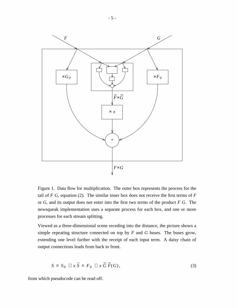
The convolution (1) has been hidden completely; all the necessary bookkeeping and

storage management is embodied in the topology and contents of the auxiliary streams.

Streams fan out to feed multiple consumers. For instance G enters into both f*G and

F*G. The topology ramifies as the recursion progresses; more auxiliary streams appear

at every stage, making the recursive picture of Figure 1. To write the program, though,

we need not think about the topology, for the program is a direct image of the

mathematics (2), and the mathematics is simple.

Substitution. Substitution, or composition, of power series, defined by S = F(G), may

be done similarly, using multiplication as a subprocess. The recursive formulation is

S 0 + x S_

= F 0 + (G 0 + x G_ _

) F_ _

(G 0 + x G_ _

).

Equate coefficients to find the constant term,

S 0 = F 0 + G 0. ( first term of F

_ _(G) ).

Induction shows that in general S 0 is an infinite sum.

S 0 =i = 0Σ∞

F i G0i .

To keep the problem finite, we further stipulate that G 0 = 0. Now

- 5 -

F_ _

×G_ _

× x

+

F×G

×G 0 ×F 0

F G

Figure 1. Data flow for multiplication. The outer box represents the process for the

tail of F G, equation (2). The similar inner box does not receive the first terms of F

or G, and its output does not enter into the first two terms of the product F G. The

newsqueak implementation uses a separate process for each box, and one or more

processes for each stream splitting.

Viewed as a three-dimensional scene receding into the distance, the picture shows a

simple repeating structure connected on top by F and G buses. The buses grow,

extending one level further with the receipt of each input term. A daisy chain of

output connections leads from back to front.

S = S 0 + x S_

= F 0 + x G_ _

F_ _

(G) , (3)

from which pseudocode can be read off.

- 6 -

# calculate power series S = F(G)

put(get(F), S) # F 0

let FG = F(G) # the recursion, F_ _

(G)

let g = get(G) # discard the first term (must be 0)

let GF = G*FG # G_ _

F_ _

(G)

loop forever

put(get(GF), S)

A subtlety: the G in let FG = F(G) stands for the whole power series, while the G in

let GF = G*FG stands only for the tail G_ _

. In the same way, the meaning of F

changes between get(F) and let FG = F(G).

Exponentiation. We wish to compute X = e F . From the recursive representation,

X = e F 0 e x F_ _

, (4)

we see that

X = e F 0 . ( 1 + terms in x).

To make the constant term of X rational, we further require that F 0 = 0. Hence X 0 = 1.

Unfortunately equation (4) does not lead to an algorithm. Formal substitution yields

X(x) = 1 . X(x X_ _

). (5)

Since the first term of X(x) depends on the first term of X(x X_ _

), we are stuck in an

infinite regress. By induction we may conclude that the first term is an infinite product of

ones, but what are the higher terms? We can ‘‘cheat,’’ and substitute F in the known

power series for the exponential. It is more satisfying, though, to build from nothing and

let the program ‘‘discover’’ the exponential for itself.

A neat trick suffices. The identity,

X ′ =dxd_ __e F = e F F ′ = X F ′ ,

may be read as a differential equation for X, with the formal solution,

X(x) =0∫x

X( t) F ′ ( t) dt + c ,

- 7 -

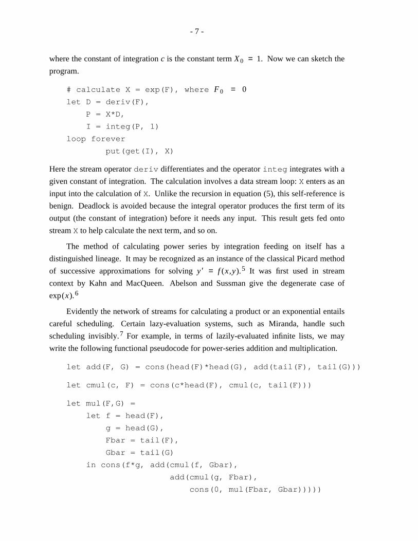
where the constant of integration c is the constant term X 0 = 1. Now we can sketch the

program.

# calculate X = exp(F), where F 0 = 0

let D = deriv(F),

P = X*D,

I = integ(P, 1)

loop forever

put(get(I), X)

Here the stream operator deriv differentiates and the operator integ integrates with a

given constant of integration. The calculation involves a data stream loop: X enters as an

input into the calculation of X. Unlike the recursion in equation (5), this self-reference is

benign. Deadlock is avoided because the integral operator produces the first term of its

output (the constant of integration) before it needs any input. This result gets fed onto

stream X to help calculate the next term, and so on.

The method of calculating power series by integration feeding on itself has a

distinguished lineage. It may be recognized as an instance of the classical Picard method

of successive approximations for solving y ′ = f (x ,y).5 It was first used in stream

context by Kahn and MacQueen. Abelson and Sussman give the degenerate case of

exp (x).6

Evidently the network of streams for calculating a product or an exponential entails

careful scheduling. Certain lazy-evaluation systems, such as Miranda, handle such

scheduling invisibly.7 For example, in terms of lazily-evaluated infinite lists, we may

write the following functional pseudocode for power-series addition and multiplication.

let add(F, G) = cons(head(F)*head(G), add(tail(F), tail(G)))

let cmul(c, F) = cons(c*head(F), cmul(c, tail(F)))

let mul(F,G) =

let f = head(F),

g = head(G),

Fbar = tail(F),

Gbar = tail(G)

in cons(f*g, add(cmul(f, Gbar),

add(cmul(g, Fbar),

cons(0, mul(Fbar, Gbar)))))

- 8 -

These functions follow from the same recursive equations as did the previous

pseudocode, with head and cons playing the role of get and put.

Lazily-evaluated languages are, alas, not widely disseminated. Moreover, they do

not inherently offer control over the exploitation of parallelism. An alternative exists in

CSP languages. These languages require some infrastructure to be built to handle the

scheduling. Once that is done, it becomes possible to write more efficient (though more

verbose) code in CSP style. We shall return to this comparison at the end of the paper.

In the meantime we proceed to an implementation in a channel-based CSP language.

Translation to newsqueak

Pike’s newsqueak language supports asynchronous processes communicating over

typed channels. Channels and functions are first-class citizens. Values of both kinds

may be assigned to variables, passed as arguments, and returned by functions. Processes

and channels may be created at will. There is just one kind of interprocess

communication—rendezvous of two processes on a channel. Consequently the queuing

and fanout that are necessary for power series computations must be programmed

explicitly. A fair choice is made among competing rendezvous. When not waiting for

rendezvous, all processes progress, at dithered rates, a few atomic operations per

interpreter cycle.

Most of newsqueak will be familiar to experienced programmers. The

communication semantics descends mainly from CSP,1 the syntax from C, and the type

system from Pascal and ML.8 Unusual features will be described as they are needed. For

details see the accompanying paper and the manual.3, 9

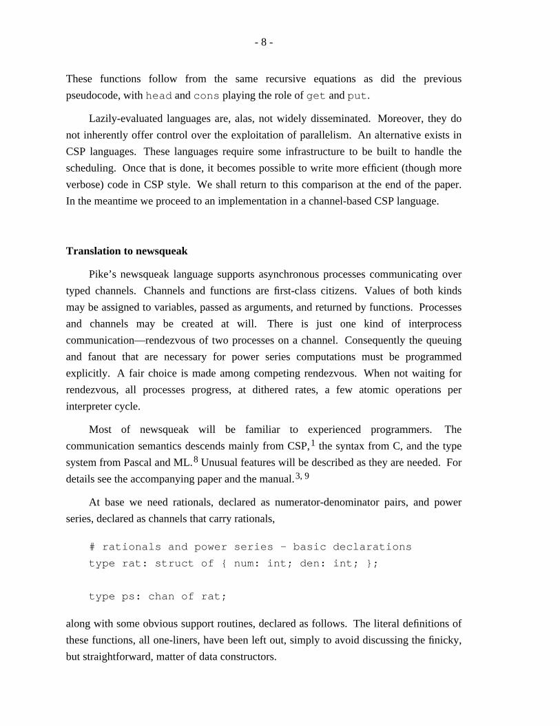
At base we need rationals, declared as numerator-denominator pairs, and power

series, declared as channels that carry rationals,

# rationals and power series - basic declarations

type rat: struct of { num: int; den: int; };

type ps: chan of rat;

along with some obvious support routines, declared as follows. The literal definitions of

these functions, all one-liners, have been left out, simply to avoid discussing the finicky,

but straightforward, matter of data constructors.

- 9 -

ratmk: prog(i:int, j:int) of rat; # construct a rational i/j

ratadd: prog(r:rat, s:rat) of rat; # return sum of rationals

ratsub: prog(r:rat, s:rat) of rat; # subtract

ratmul: prog(r:rat, s:rat) of rat; # multiply

ratprint: prog(r:rat); # print a rational

psmk: prog() of ps; # construct a power series

A program to print (endlessly) a power series is easy. To write it, though, we need

some peculiar newsqueak syntax. Beware, in newsqueak := is not a simple assignment.

It declares and initializes a new variable of a type inferred from the initializing

expression. Assignment is represented by = as in C. The prefix operator <- corresponds

to get. A prog declarator followed by a body in braces {} denotes a value of function

or procedure type. The printing program, which never terminates, is a procedure. It is

given as the initial value of psprint, which consequently becomes a procedure.

# print power series F

psprint:= prog(F:ps) {

for(;;) # loop forever

ratprint(<-F);

};

Adding power series is not much harder. We need one more operator, <-=, which

plays the role of put.

# calculate power series S = F + G

do_psadd:= prog(F:ps, G:ps, S:ps) {

for(;;)

S <-= ratadd(<-F, <-G);

};

This procedure must be run as a separate process, which we do by invoking it in a

begin statement.†

S:= psmk();

begin do_psadd(F, G, S); # start a process

psprint(S);

† In newsqueak begin is a verb, not punctuation as in Pascal. It serves the same purpose as postfix & in

UNIX shells.

- 10 -

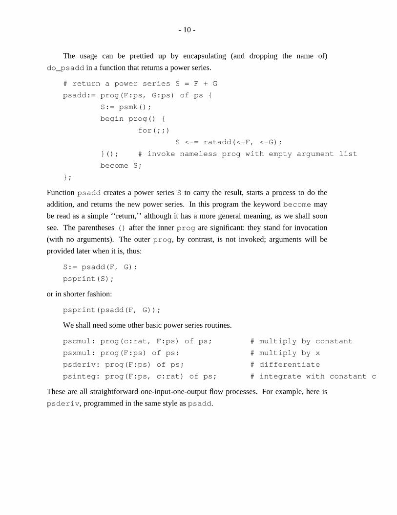
The usage can be prettied up by encapsulating (and dropping the name of)

do_psadd in a function that returns a power series.

# return a power series S = F + G

psadd:= prog(F:ps, G:ps) of ps {

S:= psmk();

begin prog() {

for(;;)

S <-= ratadd(<-F, <-G);

}(); # invoke nameless prog with empty argument list

become S;

};

Function psadd creates a power series S to carry the result, starts a process to do the

addition, and returns the new power series. In this program the keyword become may

be read as a simple ‘‘return,’’ although it has a more general meaning, as we shall soon

see. The parentheses () after the inner prog are significant: they stand for invocation

(with no arguments). The outer prog, by contrast, is not invoked; arguments will be

provided later when it is, thus:

S:= psadd(F, G);

psprint(S);

or in shorter fashion:

psprint(psadd(F, G));

We shall need some other basic power series routines.

pscmul: prog(c:rat, F:ps) of ps; # multiply by constant

psxmul: prog(F:ps) of ps; # multiply by x

psderiv: prog(F:ps) of ps; # differentiate

psinteg: prog(F:ps, c:rat) of ps; # integrate with constant c

These are all straightforward one-input-one-output flow processes. For example, here is

psderiv, programmed in the same style as psadd.

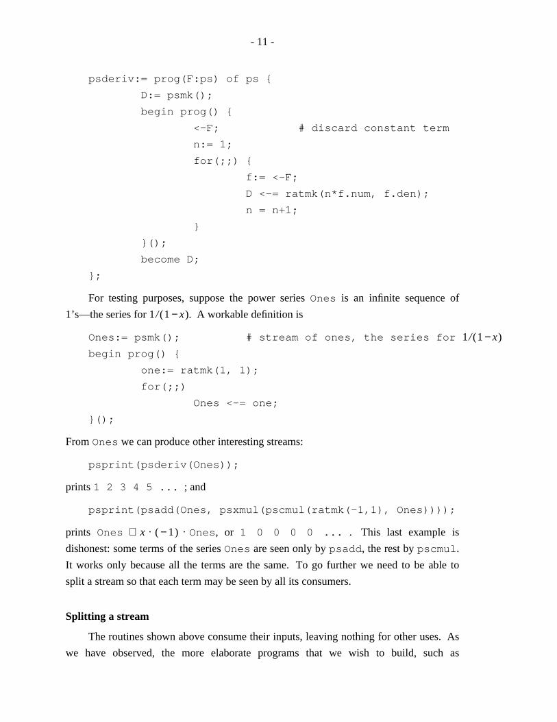
- 11 -

psderiv:= prog(F:ps) of ps {

D:= psmk();

begin prog() {

<-F; # discard constant term

n:= 1;

for(;;) {

f:= <-F;

D <-= ratmk(n*f.num, f.den);

n = n+1;

}

}();

become D;

};

For testing purposes, suppose the power series Ones is an infinite sequence of

1’s—the series for 1 /( 1 − x). A workable definition is

Ones:= psmk(); # stream of ones, the series for 1/( 1 − x)

begin prog() {

one:= ratmk(1, 1);

for(;;)

Ones <-= one;

}();

From Ones we can produce other interesting streams:

psprint(psderiv(Ones));

prints 1 2 3 4 5 ... ; and

psprint(psadd(Ones, psxmul(pscmul(ratmk(-1,1), Ones))));

prints Ones + x . ( − 1 ) . Ones, or 1 0 0 0 0 ... . This last example is

dishonest: some terms of the series Ones are seen only by psadd, the rest by pscmul.

It works only because all the terms are the same. To go further we need to be able to

split a stream so that each term may be seen by all its consumers.

Splitting a stream

The routines shown above consume their inputs, leaving nothing for other uses. As

we have observed, the more elaborate programs that we wish to build, such as

- 12 -

multiplication of power series, need fanout. In preparation, we next design a stream-

splitting process. Since the two branches of a split stream may be read at different rates,

we shall need a queue to hold values to be read later. The queue will materialize as a

chain of processes, each holding a single value.

The program begins by reading one item from the input F. Not knowing which of

the two outputs will be read first, it waits on a select statement for whichever of the

two rendezvous cases happens first.

# calculate power series C = F (service routine for do_split)

copy:= prog(F:ps, C:ps) {

for(;;)

C <-= <-F;

};

# split power series F into F0 and F1, each the same as F

rec do_split:= prog(F:ps, F0:ps, F1:ps) {

f:= <-F;

H:= psmk(); # the held branch

select {

case F0 <-= f:

begin do_split(F, F0, H);

F1 <-= f;

become copy(H, F1);

case F1 <-= f:

# same, with F0 and F1 interchanged

}

};

The keyword rec announces that the function is recursive. When the rendezvous on F0

wins, the previously read item f is sent to F0 as part of the rendezvous action. The tail

of F is then split recursively in a separate process and the original instance of do_split

waits for a rendezvous on the other output stream F1. After that rendezvous, the process

is replaced by (becomes) a simple loop that copies from the held queue to F1.*

Once again it will be convenient to encapsulate the process, this time into a

function, split, which takes one power series and returns a pair, declared thus:

* Readers familiar with Hoare’s CSP will recognize become as the - - - > operator of CSP.1

- 13 -

type pspair: array[2] of ps; # a pair of power series

pspairmk: prog(F:ps, G:ps) of pspair; # construct a pair

split: prog(F:ps) of pspair; # return 2 copies of F

Because its definition is recursive, the name of do_split, unlike that of do_psadd,

must persist in the encapsulated version.

# return a pair of copies of power series F (consuming F)

split:= prog(F:ps) of pspair {

FF:= pspairmk(psmk(), psmk());

begin do_split(F, FF[0], FF[1]);

become FF;

};

This splitting function has deficiencies, to which we shall return. (You are invited

to try to spot them.) Nevertheless, with split, we now have the wherewithal to

program a crude version of power series multiplication. Recall the pseudocode,

let f = get(F),

g = get(G)

put(f*g, P)

let fG = f*G,

gF = g*F,

xFG = x*(F*G)

loop forever

put(get(fG) + get(gF) + get(xFG), P)

In the newsqueak version that follows, the inner prog implements the pseudocode. The

program is encapsulated as usual.

- 14 -

# return power series F*G

rec psmul:= prog(F:ps, G:ps) of ps {

P:= psmk();

begin prog(){

f := <-F;

g := <-G;

FF := split(F);

GG := split(G);

P <-= ratmul(f, g);

fG := pscmul(f, GG[0]);

gF := pscmul(g, FF[0]);

xFG := psxmul(psmul(FF[1], GG[1]));

for(;;)

P <-= ratadd(ratadd(<-fG, <-gF), <-xFG);

}();

become P;

};

This code works. For example, with Ones defined as before,

OnesOnes:= split(Ones);

psprint(psmul(OnesOnes[0], OnesOnes[1]));

prints 1 2 3 4 5 ... , the correct answer for 1 /( 1 − x)2. This time the test program

is honest: the stream Ones is split before use. Disappointingly, though, it takes a

thousand processes to produce only forty terms—and sluggishly at that. What are all

those processes doing?

Reducing overhead

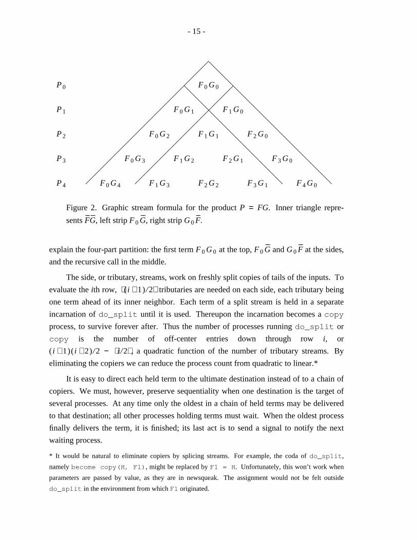
Figure 2 depicts the recursive decomposition of stream multiplication and its

relationship to the convolution formula (1). The ith row contains summands for the ith

term of the product P = FG. The full figure contains the whole product; the inner

triangle contains the product of the tails, F_ _

G_ _

; and the flanking strips contain the terms of

the series F 0 G_ _

and G 0 F_ _

. Stepping down one row corresponds to multiplication by x.

The four terms in the formula,

FG = F 0 G 0 + xF 0 G_ _

+ xG 0 F_ _

+ x 2 F_ _

G_ _

, (6)

- 15 -

F 0 G 0

F 0 G 1 F 1 G 0

F 2 G 0F 1 G 1F 0 G 2

F 0 G 3 F 1 G 2 F 2 G 1 F 3 G 0

F 4 G 0F 3 G 1F 2 G 2F 1 G 3F 0 G 4P 4

P 3

P 2

P 1

P 0

Figure 2. Graphic stream formula for the product P = FG. Inner triangle repre-

sents F_ _

G_ _

, left strip F 0 G_ _

, right strip G 0 F_ _

.

explain the four-part partition: the first term F 0 G 0 at the top, F 0 G_ _

and G 0 F_ _

at the sides,

and the recursive call in the middle.

The side, or tributary, streams, work on freshly split copies of tails of the inputs. To

evaluate the ith row, ( i + 1 )/2 tributaries are needed on each side, each tributary being

one term ahead of its inner neighbor. Each term of a split stream is held in a separate

incarnation of do_split until it is used. Thereupon the incarnation becomes a copy

process, to survive forever after. Thus the number of processes running do_split or

copy is the number of off-center entries down through row i, or

( i + 1 ) ( i + 2 )/2 − i /2 , a quadratic function of the number of tributary streams. By

eliminating the copiers we can reduce the process count from quadratic to linear.*

It is easy to direct each held term to the ultimate destination instead of to a chain of

copiers. We must, however, preserve sequentiality when one destination is the target of

several processes. At any time only the oldest in a chain of held terms may be delivered

to that destination; all other processes holding terms must wait. When the oldest process

finally delivers the term, it is finished; its last act is to send a signal to notify the next

waiting process.

* It would be natural to eliminate copiers by splicing streams. For example, the coda of do_split,

namely become copy(H, F1), might be replaced by F1 = H. Unfortunately, this won’t work when

parameters are passed by value, as they are in newsqueak. The assignment would not be felt outside

do_split in the environment from which F1 originated.

- 16 -

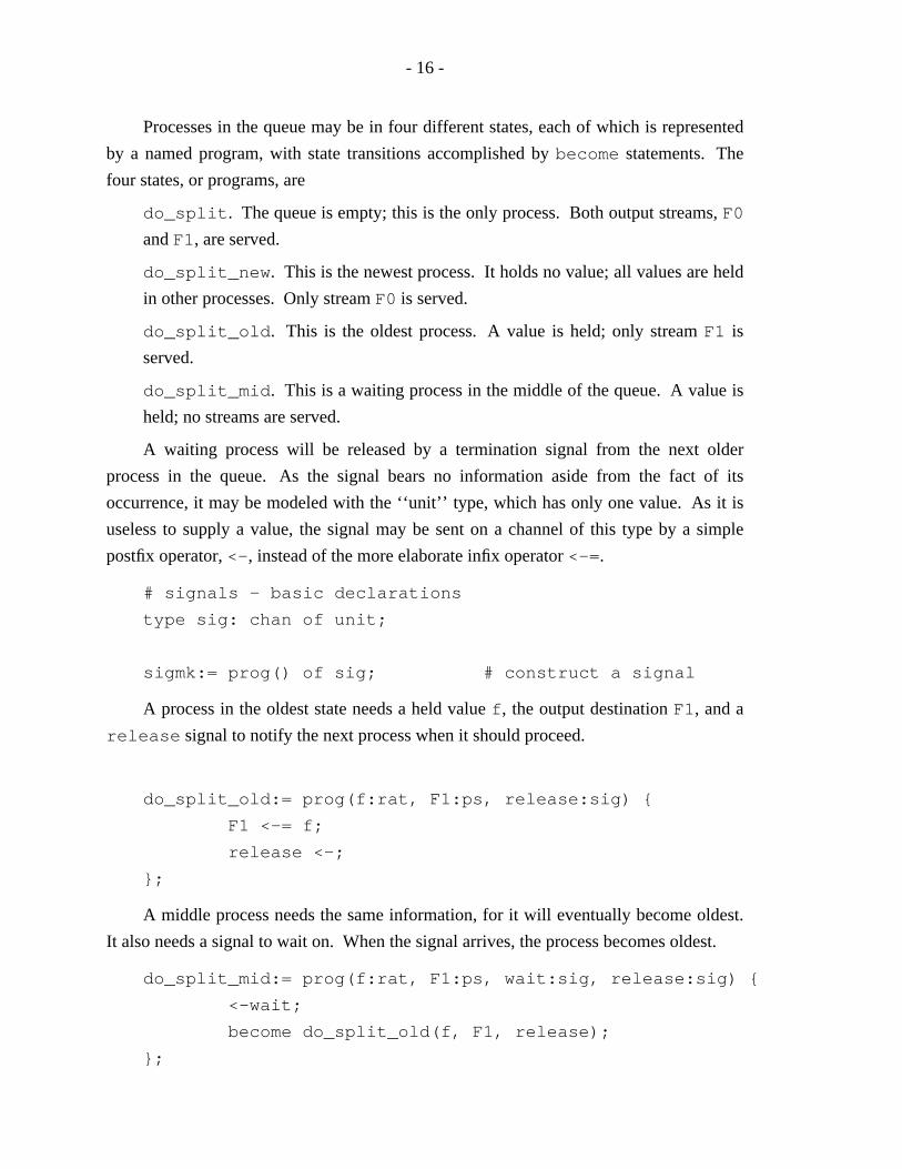
Processes in the queue may be in four different states, each of which is represented

by a named program, with state transitions accomplished by become statements. The

four states, or programs, are

do_split. The queue is empty; this is the only process. Both output streams, F0

and F1, are served.

do_split_new. This is the newest process. It holds no value; all values are held

in other processes. Only stream F0 is served.

do_split_old. This is the oldest process. A value is held; only stream F1 is

served.

do_split_mid. This is a waiting process in the middle of the queue. A value is

held; no streams are served.

A waiting process will be released by a termination signal from the next older

process in the queue. As the signal bears no information aside from the fact of its

occurrence, it may be modeled with the ‘‘unit’’ type, which has only one value. As it is

useless to supply a value, the signal may be sent on a channel of this type by a simple

postfix operator, <-, instead of the more elaborate infix operator <-=.

# signals - basic declarations

type sig: chan of unit;

sigmk:= prog() of sig; # construct a signal

A process in the oldest state needs a held value f, the output destination F1, and a

release signal to notify the next process when it should proceed.

do_split_old:= prog(f:rat, F1:ps, release:sig) {

F1 <-= f;

release <-;

};

A middle process needs the same information, for it will eventually become oldest.

It also needs a signal to wait on. When the signal arrives, the process becomes oldest.

do_split_mid:= prog(f:rat, F1:ps, wait:sig, release:sig) {

<-wait;

become do_split_old(f, F1, release);

};

- 17 -

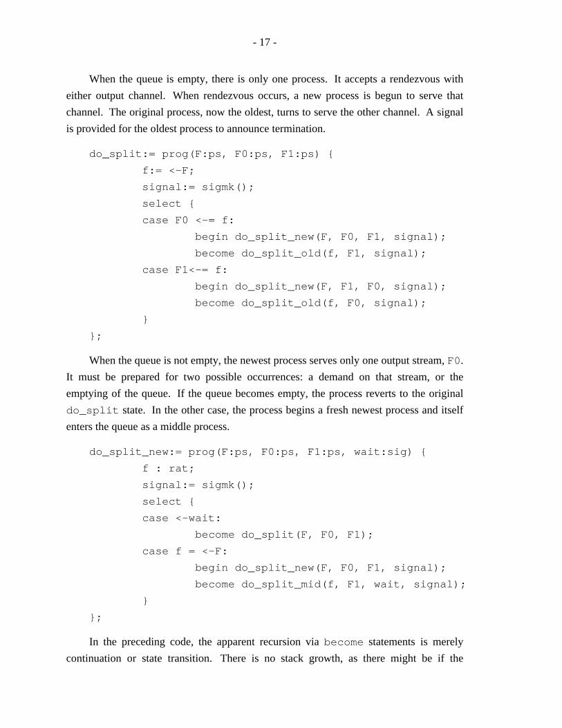
When the queue is empty, there is only one process. It accepts a rendezvous with

either output channel. When rendezvous occurs, a new process is begun to serve that

channel. The original process, now the oldest, turns to serve the other channel. A signal

is provided for the oldest process to announce termination.

do_split:= prog(F:ps, F0:ps, F1:ps) {

f:= <-F;

signal:= sigmk();

select {

case F0 <-= f:

begin do_split_new(F, F0, F1, signal);

become do_split_old(f, F1, signal);

case F1<-= f:

begin do_split_new(F, F1, F0, signal);

become do_split_old(f, F0, signal);

}

};

When the queue is not empty, the newest process serves only one output stream, F0.

It must be prepared for two possible occurrences: a demand on that stream, or the

emptying of the queue. If the queue becomes empty, the process reverts to the original

do_split state. In the other case, the process begins a fresh newest process and itself

enters the queue as a middle process.

do_split_new:= prog(F:ps, F0:ps, F1:ps, wait:sig) {

f : rat;

signal:= sigmk();

select {

case <-wait:

become do_split(F, F0, F1);

case f = <-F:

begin do_split_new(F, F0, F1, signal);

become do_split_mid(f, F1, wait, signal);

}

};

In the preceding code, the apparent recursion via become statements is merely

continuation or state transition. There is no stack growth, as there might be if the

- 18 -

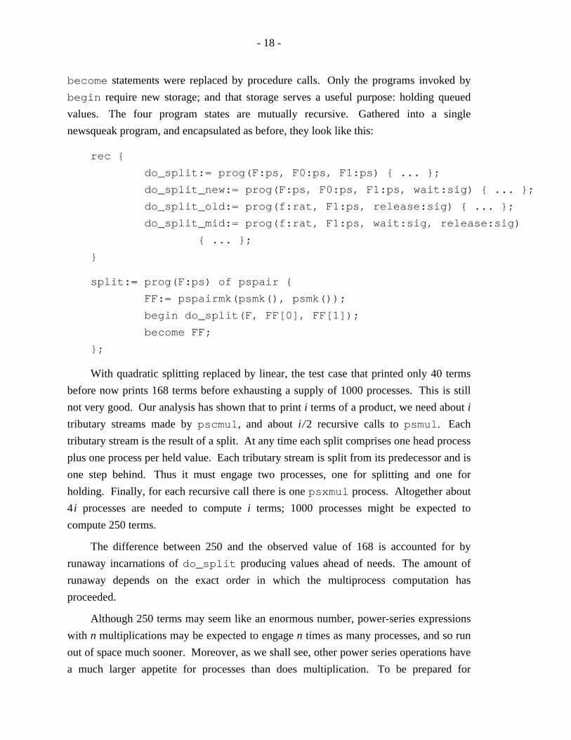
become statements were replaced by procedure calls. Only the programs invoked by

begin require new storage; and that storage serves a useful purpose: holding queued

values. The four program states are mutually recursive. Gathered into a single

newsqueak program, and encapsulated as before, they look like this:

rec {

do_split:= prog(F:ps, F0:ps, F1:ps) { ... };

do_split_new:= prog(F:ps, F0:ps, F1:ps, wait:sig) { ... };

do_split_old:= prog(f:rat, F1:ps, release:sig) { ... };

do_split_mid:= prog(f:rat, F1:ps, wait:sig, release:sig)

{ ... };

}

split:= prog(F:ps) of pspair {

FF:= pspairmk(psmk(), psmk());

begin do_split(F, FF[0], FF[1]);

become FF;

};

With quadratic splitting replaced by linear, the test case that printed only 40 terms

before now prints 168 terms before exhausting a supply of 1000 processes. This is still

not very good. Our analysis has shown that to print i terms of a product, we need about i

tributary streams made by pscmul, and about i /2 recursive calls to psmul. Each

tributary stream is the result of a split. At any time each split comprises one head process

plus one process per held value. Each tributary stream is split from its predecessor and is

one step behind. Thus it must engage two processes, one for splitting and one for

holding. Finally, for each recursive call there is one psxmul process. Altogether about

4i processes are needed to compute i terms; 1000 processes might be expected to

compute 250 terms.

The difference between 250 and the observed value of 168 is accounted for by

runaway incarnations of do_split producing values ahead of needs. The amount of

runaway depends on the exact order in which the multiprocess computation has

proceeded.

Although 250 terms may seem like an enormous number, power-series expressions

with n multiplications may be expected to engage n times as many processes, and so run

out of space much sooner. Moreover, as we shall see, other power series operations have

a much larger appetite for processes than does multiplication. To be prepared for

- 19 -

expressions of more complexity, we cannot use processes recklessly. Runaways are the

major remaining profligacy; to prevent them we must attend to scheduling.

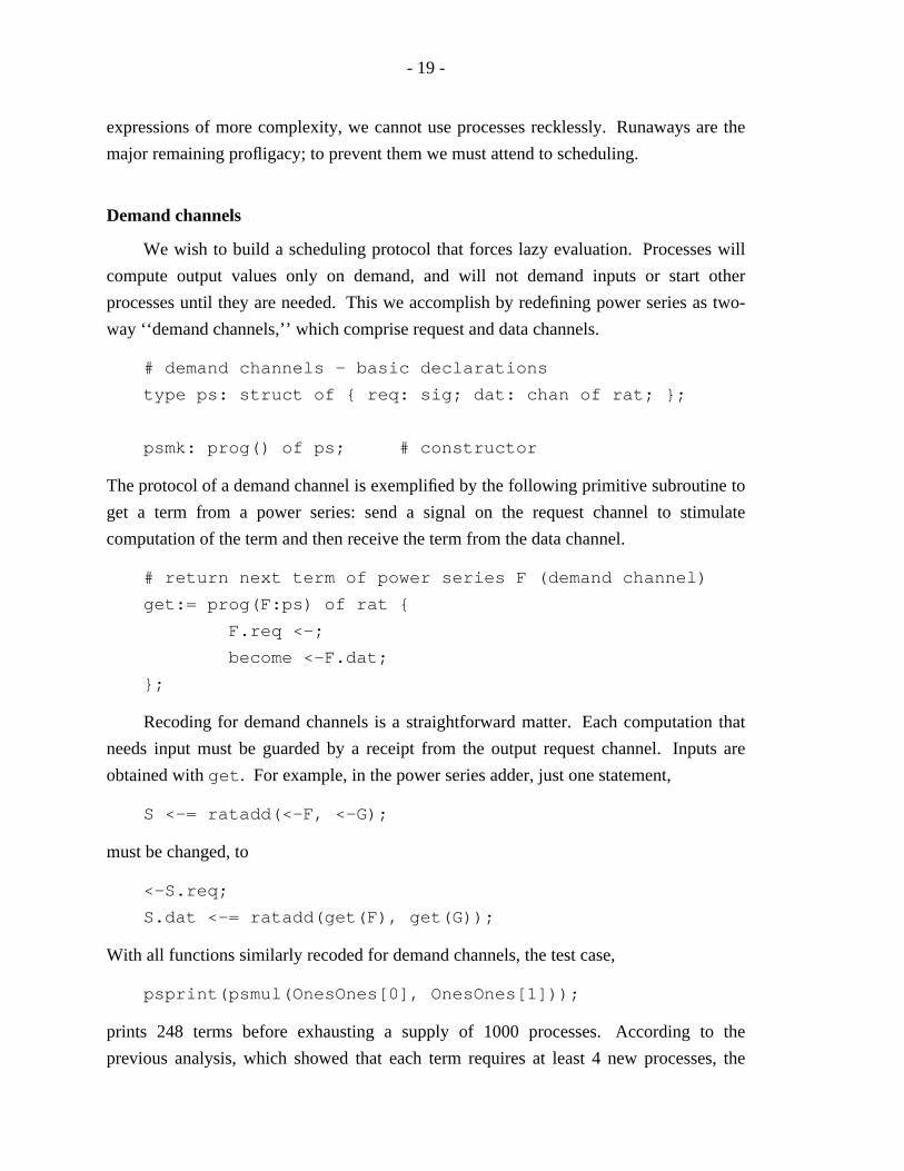
Demand channels

We wish to build a scheduling protocol that forces lazy evaluation. Processes will

compute output values only on demand, and will not demand inputs or start other

processes until they are needed. This we accomplish by redefining power series as two-

way ‘‘demand channels,’’ which comprise request and data channels.

# demand channels - basic declarations

type ps: struct of { req: sig; dat: chan of rat; };

psmk: prog() of ps; # constructor

The protocol of a demand channel is exemplified by the following primitive subroutine to

get a term from a power series: send a signal on the request channel to stimulate

computation of the term and then receive the term from the data channel.

# return next term of power series F (demand channel)

get:= prog(F:ps) of rat {

F.req <-;

become <-F.dat;

};

Recoding for demand channels is a straightforward matter. Each computation that

needs input must be guarded by a receipt from the output request channel. Inputs are

obtained with get. For example, in the power series adder, just one statement,

S <-= ratadd(<-F, <-G);

must be changed, to

<-S.req;

S.dat <-= ratadd(get(F), get(G));

With all functions similarly recoded for demand channels, the test case,

psprint(psmul(OnesOnes[0], OnesOnes[1]));

prints 248 terms before exhausting a supply of 1000 processes. According to the

previous analysis, which showed that each term requires at least 4 new processes, the

- 20 -

scheduling is optimal. To improve matters further, we must reduce the per-term

requirements.

The newest in a chain of do_split processes does not pull full weight, for it

contains no held value. For this reason, with optimal scheduling, every tributary stream

in psmul was observed to engage two processes. The two processes may be reduced to

one by letting the newest process hold the first value and distinguishing two states of the

process, one ‘‘full’’ and one ‘‘empty.’’ Furthermore, by coding psxmul in-line in

psmul, a further process may be avoided for each recursion level, or one for each two

output terms. At the outer level of Figure 1, there would remain one process for the

enclosing box, one for each of the left and right inner boxes, and a splitting process for

each of the two inputs. These improvements will bring the process count down to 2.5 per

output term.

Other operations

Substitution of power series. We have already seen (3) that the substitution S = F(G),

where G 0 = 0, may be computed from the formula

S = S 0 + x S_

= F 0 + x G_ _

F_ _

(G) .

The corresponding newsqueak code is

# return F(G), where G 0 = 0.

rec pssubst:= prog(F:ps, G:ps) of ps {

S:= psmk();

begin prog() {

GG:= split(G);

<-S.req;

S.dat <-= get(F);

get(GG[0]);

become copy(psmul(GG[0], pssubst(F, GG[1])), S);

}();

become S;

};

This code, like the original do_split, leaves a copier at every stage of recursion. The

copiers here, however, are not cascaded, so there is only a constant, rather than an O(n),

factor to be gained from eliminating them.

- 21 -

Exponential of a power series. From the previously derived pseudocode,

let D = deriv(F),

P = X*D,

I = integ(P, 1)

loop forever

put(get(I), X)

comes the following newsqueak program. The call for copy is no cause for alarm,

because there is no recursion.

# exponential of power series X = exp(F) where F 0 = 0

psexp:= prog(F:ps) of ps {

X:= psmk();

XX:= split(X);

I:= psinteg(psmul(XX[0], psderiv(F)), ratmk(1, 1));

begin copy(I, X);

become XX[1];

};

Reciprocal of a power series; find R such that F R = 1. Expand F to obtain

(F 0 + x F_ _

) R = 1 ,

or

R = R 0 + x R_ _

=F 0

1___ ( 1 − x F_ _

R).

From this formula we see that the reciprocal has the same computational complexity as

multiplication. We may also read off a translation into newsqueak.

- 22 -

ratneg: prog(r:rat) of rat; # negate a rational

ratrecip: prog(r:rat) of rat; # reciprocal of a rational

# return power series 1/F

psrecip:= prog(F:ps) of ps {

R:= psmk();

RR:= split(R);

begin prog() {

<-R.req;

g:= ratrecip(get(F));

R.dat <-= g;

become copy(pscmul(ratneg(g), psmul(F, RR[0])), R);

}();

become RR[1];

};

Reversion of power series. Find the functional inverse of power series F. That is, find R

such that

F(R(x) ) = x. (7)

From equating coefficients we find that R 0 must satisfy

i = 0Σ∞

F i R0i = 0 ,

that is, R 0 must be a root of F. To keep the coefficients of R rational, we stipulate that

R 0 = 0. Hence also F 0 = 0. Thus we assume that F has the form

F(x) = x F_ _

= x F 1 + x 2 F_ __ _

,

and similarly for R. The basic identity (7) becomes

x R_ _

F_ _

(R) = x.

Expand F and solve for R_ _

(which may also be written R 1 + x R_ __ _

).

x R_ _

(F 1 + x R_ _

F_ __ _

(R) ) = x ,

R_ _

= R 1 + x R_ __ _

=F 1

1___ ( 1 − x R_ _

2 F_ __ _

(R) ). (8)

- 23 -

Since R 0 is zero, the substitution F_ __ _

(R) satisfies the precondition of pssubst, and that

procedure may be used. Counting R_ _

2 as two appearances, R appears three times in the

right side of (8); the newsqueak program must involve three splits. Otherwise it is like

all the rest, and so will be omitted.

As an example of the use of reversion, consider calculating tan (x) from its simpler

inverse function arctan (x). The arctangent has an easy derivative,

dxd_ __ arctan (x) =

1 + x 21_ ______ .

Posit a monomial substitution operator, psmsubst(F, c, n), that calculates

F(cx n ).* Substitute − x 2 into Ones (i.e. into 1 /( 1 − x)) to get 1 /( 1 + x 2 ), integrate to

get the arctangent, and revert. The resulting code,

psmsubst : prog(ps, rat, int) of ps; # monomial substitution

psrev : prog(ps) of ps; # reversion

Tan:= psrev(psinteg(psmsubst(Ones, ratmk(-1, 1), 2), 0));

psprint(Tan);

prints the coefficients of the tangent series:

0 1 0 1/3 0 2/15 0 17/315 0 62/2835 0 1382/155925 ...

Various algorithms and formulas for reversion may be found in the literature.10, 11

None that I have seen are as straightforward as (8), which completely hides the

combinatoric complexity, yet constitutes a detailed specification for a program. One

could not ask for a better testimonial for stream methods.

Complexity

The complexity of the several stream operations may be derived from their defining

equations. For definiteness, we shall count the number of coefficient-domain products

necessary to compute coefficients of x 0, x 1, ..., x n in an output series.

Multiplication. Let Prod (n) denote the desired count. From (6)

P = FG = F 0 G 0 + xF 0 G_ _

+ xG 0 F_ _

+ x 2 F_ _

G_ _

.

To compute terms P 0 through P n , we need

* This simple operator multiplies each input coefficient F i by c i and copies it to the output followed by

n − 1 zeros.

- 24 -

the single product F 0 G 0,

if n ≥ 1, terms of F 0 G_ _

and G 0 F_ _

through x n − 1, and

if n ≥ 2, terms of F_ _

G_ _

through x n − 2.

Thus Prod (n) satisfies

Prod (n) = 1 + 2n + Prod (n − 2 ) , n ≥ 2 ,

Prod ( 1 ) = 3

Prod ( 0 ) = 1

or, in closed form,

Prod (n) = 2n + 2

= O(n 2 ).

Thus, if rational operations are counted as unit time, stream multiplication takes

quadratic time. Space, as measured by the process count, is also linear.

Substitution. From (3), we have

S = F(G) = F 0 + x G_ _

F_ _

(G).

To compute S 0 through S n , where n ≥ 1, we need

terms of F_ _

(G) through x n − 1, and

terms of the product G_ _

F_ _

(G) through x n − 1,

whence the desired count, Subst (n), satisfies

Subst (n) = Subst (n − 1 ) + Prod (n − 1 ) , n ≥ 1 ,

Subst ( 0 ) = 0 ,

with the closed form solution

Subst (n) = 3n + 2

= O(n 3 ).

Reversion. From (8), the solution R of F(R(x) ) = x satisfies

R =F 1

x___ ( 1 − x R_ _

2 F_ __ _

(R) ).

To compute R 0 through R n , where n ≥ 2, we need

- 25 -

terms of F_ __ _

(R) through x n − 2,

terms of two power series products through x n − 2, and

n − 1 termwise multiplications by 1 / F 1.

The desired count, Rev (n), satisfies

Rev (n) = n − 1 + 2 Prod (n − 2 ) + Subst (n − 2 ) , n ≥ 2.

Rev ( 0 ) = Rev ( 1 ) = 0 ,

Substituting and simplifying, we find that reversion and substitution are equally difficult

in this measure:

Rev (n) = 3n + 2

− 1 = O(n 3 ) , n ≥ 1.

Exponentiation, reciprocation. Both operations require O(n 2 ) coefficient-domain

products.

Discussion

The method here demonstrated calculates the coefficients of power series defined by

sets of recursive equations, provided the equations express later terms in terms of earlier

ones. We have seen how such recursive equations can be translated straightforwardly

into stream-processing programs. In doing the translation, two technical difficulties were

encountered. The first, the necessity for fanout and queuing, was solved by a splitting

function. The second, minimizing computation in excess of the needs of the ultimate

consumer, was solved by demand channels.

The stream algorithms realize the same complexity as other power series algorithms

with the ‘‘sequential’’ property of producing n terms of output without accessing more

than n + k terms of input for some fixed k.11 Although more efficient nonsequential

algorithms are known,12 the stream formulation remains attractive by reason of its

extreme simplicity. The availability of such programming techniques would simplify the

organization of symbolic calculations, which are central in systems like Macsyma or

Maple, and are beginning to make their way into numerical algorithms.

The style of programming used here was first articulated by Landin, who described

a data stream in applicative terms as a function that returns a pair comprising the first

element of the stream and a continuation. The continuation is another function of the

same type.13 To get the second element, invoke the continuation. It will deliver another

continuation for further reference, and so on. Channels may be understood as Landin

- 26 -

stream variables. A process receiving from a channel effectively invokes the

continuation and stores the continuation part of the result back into the channel. The

corresponding sender, however, is at liberty to calculate ahead in preparation for the next

rendezvous. Herein lies the potential for runaway, which was cured by using demand

channels. Demand channels enforce the most literal interpretation of the Landin model,

where future needs are never anticipated.

Besides giving us a way to describe stream processes, the Landin model gives us a

way to think about them. The first-plus-tail style of mathematical analysis, as a perfect

match to the first-plus-continuation model of streams, leads directly to useful and

otherwise nonobvious stream algorithms. First-plus-tail analysis, of course, may be used

in stream applications other than power series. For example, Kahn and MacQueen

mention unlimited-precision computation with reals, where streams carry the digits.4 In a

domain of infinite sequences, recursive equations are a mode of expression as natural as

arithmetic formulas are in a scalar domain.

As we have seen, infinite lists, which underlie lazy evaluation systems, constitute an

alternative to data stream representations. Recursive equations lead somewhat more

directly to programs on infinite lists than on channels, as lazy-evaluation systems already

contain the infrastructure to handle fanout and scheduling. But once the infrastructure is

built and hidden, programs in the two kinds of systems look quite similar. The

newsqueak program for the tangent,

Tan:= psrev(psinteg(psmsubst(Ones, ratmk(-1, 1), 2), 0));

looks just as it would in any other functional language. For comparison, I programmed

the application in ML,14 using a lazy-stream module written by David MacQueen. The

ML source code was about half the size of the newsqueak.* However, the compiled ML

ran only one-fifth as fast as the interpreted newsqueak. Channels make a difference.

As stream processing makes its way into mainstream languages, the style of

programming illustrated here will become increasingly important.

* The following example of the ML code may be compared with the reciprocal operator given under

‘‘Other operations’’ above. The notation fn()=> introduces a lambda expression for a pair-valued Landin

function.

fun psrecip F =

let val g = ratrecip(head F) in

let fun psrecip’() = lazyCons(fn() =>

(g, pscmul(ratneg g, psmul(tail F, psrecip’())))) in

psrecip’() end end;

- 27 -

I am grateful to Gilles Kahn for introducing me to this elegant application, to Jon

Bentley for bringing me up to date on complexity matters, to Dave MacQueen for

semantic insight and assistance with ML, and to Rob Pike for tuning squint to meet the

stresses of the application and for thoughtful advice on drafts of this paper.

- 28 -

References

[1] Hoare, C. A. R., Communicating Sequential Processes, Prentice-Hall, Englewood

Cliffs, NJ (1985).

[2] Hehner, E. C. R., Logic of Programming, Prentice-Hall (1984).

[3] Pike, R., ‘‘The Implementation of Newsqueak,’’ Software(emPractice and

Experience (this issue).

[4] Kahn, G. and MacQueen, D. B., ‘‘Coroutines and Networks of Parallel

Processes,’’ Information Processing 77, Proceedings of IFIP Congress 77 7, pp.

993-998, Gilchrist, B. (Ed.), North-Holland, Amsterdam (1977).

[5] Ford, L. R., Differential Equations, McGraw-Hill (1955).

[6] Abelson, H. and Sussman, G. J., Structure and Interpretation of Computer

Programs, MIT Press, Cambridge, MA (1985).

[7] Turner, D., ‘‘An Overview of Miranda,’’ ACM SIGPLAN Notices 21(12)

(December, 1986).

[8] Wikstrom, A., Functional Programming Using Standard ML, Prentice-Hall,

Englewood Cliffs, NJ (1987).

[9] Pike, R., ‘‘Newsqueak: A Language for Communicating with Mice,’’ CSTR 143,

AT&T Bell Laboratories, Murray Hill, NJ (1989).

[10] Van Orstrand, C. E., ‘‘Reversion of Power Series,’’ London, Edinburgh, and

Dublin Philosophical Magazine 19(109), pp. 366-376 (1910).

[11] Knuth, D. E., The Art of Computer Programming, Vol. 2, Addison-Wesley,

Reading, MA (1969). §4.7.

[12] Brent, R. P. and Kung, H. T., ‘‘Fast Algorithms for Manipulating Formal Power

Series,’’ JACM 25, pp. 581-595 (1978).

[13] Landin, P. J., ‘‘A Correspondence between ALGOL 60 and Church’s Lambda

Notation, Part I,’’ CACM 8, pp. 89-101 (1965).

[14] Harper, R., Milner, R., and Tofte, M., The Definition of Standard ML, MIT Press

(1990).