Application of Recognition Input Squinting and Error-Correcting Output

Coding to Convolutional Neural Networks

George Stathopoulos

A Thesis

in

The Department

of

Computer Science and Software Engineering

Presented in Partial Fulfillment of the Requirementsfor the Degree of Master in Computer Science at

Concordia UniversityMontreal, Quebec, Canada

August 2011

c⃝ George Stathopoulos, 2011

CONCORDIA UNIVERSITY

School of Graduate Studies

This is to certify that the thesis prepared

By: George Stathopoulos

Entitled: Application of Recognition Input Squinting and Error-Correcting Output Coding to Convolutional Neural Networks

and submitted in partial fulfillment of the requirements for the degree of

Master of Computer Science

complies with the regulations of the University and meets the accepted standardswith respect to originality and quality.

Signed by the final examining committee:

ChairDr. D. Goswami

ExaminerDr. A. Krzyzak

ExaminerDr. L. Lam

SupervisorDr. C. Y. Suen

Approved byChair of Department or Graduate Program Director

20Dr. Robin A. L. Drew, DeanFaculty of Engineering and Computer Science

ABSTRACT

Application of Recognition Input Squinting and Error-Correcting Output

Coding to Convolutional Neural Networks

George Stathopoulos

The Convolutional Neural Network (CNN) is a type of artificial neural network that is

successful in addressing many computer vision classification problems. This thesis considers

problems related to optical character recognition by CNN when few training samples are

available. Two techniques are proposed that can be used to improve the application of

CNNs to such problems and these benefits are demonstrated experimentally on subsets

of two labelled databases: MNIST (handwritten digits) and CENPARMI-MPC (machine-

printed characters).

The first technique is novel and is called “Recognition Input Squinting”. It involves

taking the input image to be recognized and applying a set of geometric transformations

on it to produce a set of squinted images. The trained CNN classifier then recognizes each

of these generated input images and computes an overall recognition confidence score. It

is shown that this technique yields superior recognition precision as compared to the case

where a single input image is recognized without squinting.

The second technique is an application of the Error-Correcting Output Coding technique

to the CNN. Each class to be recognized is assigned a codeword from an appropriately

chosen error-correcting code’s codebook and the CNN is trained using these codeword

labels. At recognition time, the output class is selected according to a minimum code

distance criterion. It is shown that this technique provides better recognition precision

than when the classic place output coding is used.

iii

ACKNOWLEDGEMENTS

I would like to express my sincere thanks to my supervisor Dr. Ching Y. Suen for his

guidance, patience and support over the last few years.

I would also like to thank Dr. Huiqun Deng for her encouraging words and advice.

Finally I would also like to extend my thanks to all my other CENPARMI colleagues.

It has been an honour and a privilege to be a part of such a close-knit academic family.

iv

DEDICATION

I dedicate this thesis to my family that has been by my side from the beginning.

v

TABLE OF CONTENTS

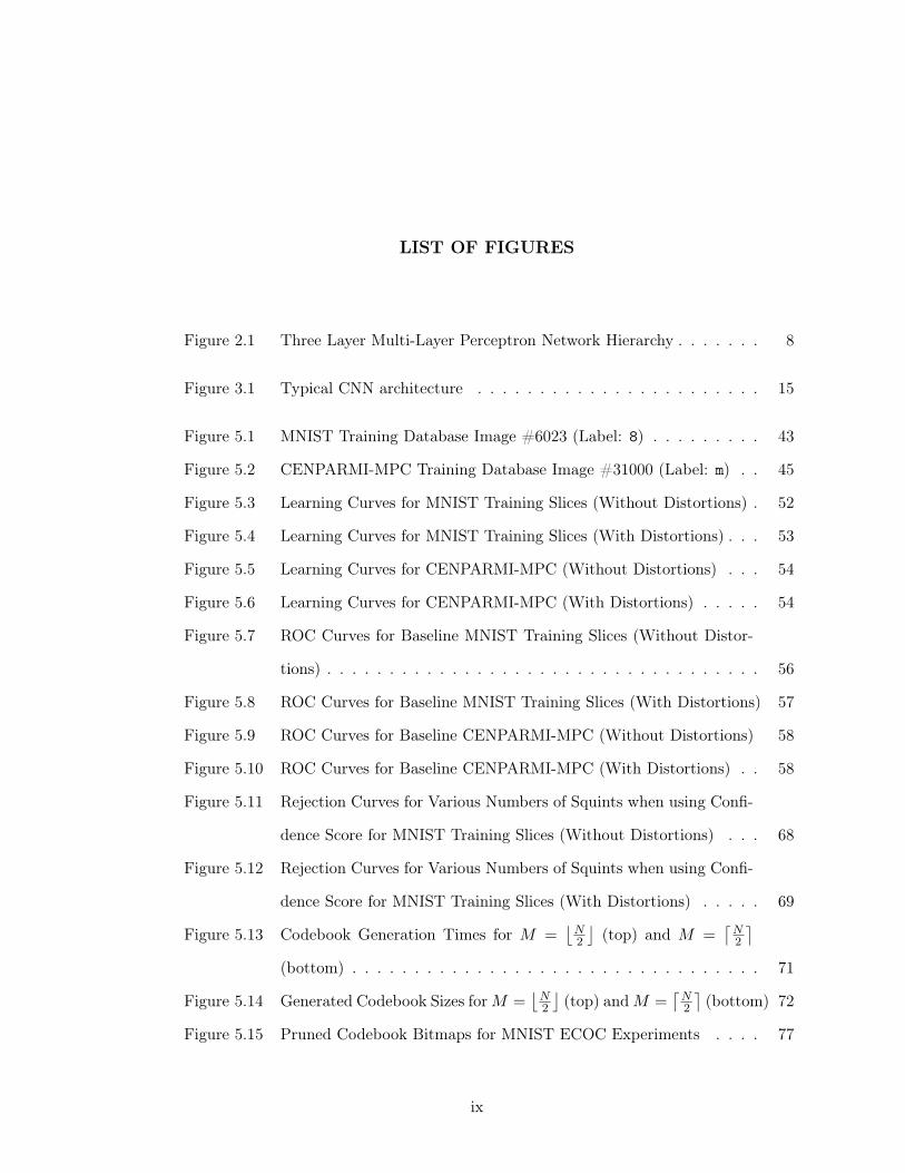
LIST OF FIGURES . . . . . . . . . . . . . . . . . . . . . . . . . . . . . . . . ix

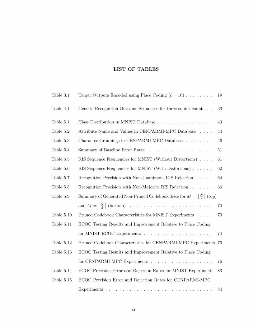
LIST OF TABLES . . . . . . . . . . . . . . . . . . . . . . . . . . . . . . . . . xi

CHAPTER 1. INTRODUCTION . . . . . . . . . . . . . . . . . . . . . . . 1

1.1 The Image Recognition Problem . . . . . . . . . . . . . . . . . . . . . . . . 1

1.2 Application of CNNs to the Image Recognition Problem . . . . . . . . . . . 3

1.3 Improving CNN Image Recognition . . . . . . . . . . . . . . . . . . . . . . . 3

1.4 Thesis Organization . . . . . . . . . . . . . . . . . . . . . . . . . . . . . . . 5

CHAPTER 2. BACKGROUND INFORMATION . . . . . . . . . . . . . . 6

2.1 Feed-Forward Artificial Neural Networks . . . . . . . . . . . . . . . . . . . . 6

2.1.1 The Perceptron . . . . . . . . . . . . . . . . . . . . . . . . . . . . . . 6

2.1.2 The Multi-Layer Perceptron Neural Network . . . . . . . . . . . . . 7

2.1.3 Artificial Neural Network Training Considerations . . . . . . . . . . 10

2.2 Error-Correcting Codes . . . . . . . . . . . . . . . . . . . . . . . . . . . . . 10

2.2.1 Linear Binary Error-Correcting Codes . . . . . . . . . . . . . . . . . 11

2.2.2 Hard Decoding vs Soft Decoding . . . . . . . . . . . . . . . . . . . . 11

CHAPTER 3. CONVOLUTIONAL NEURAL NETWORKS . . . . . . . 13

3.1 Motivation . . . . . . . . . . . . . . . . . . . . . . . . . . . . . . . . . . . . . 13

3.2 CNN Applications . . . . . . . . . . . . . . . . . . . . . . . . . . . . . . . . 14

3.3 CNN Architecture . . . . . . . . . . . . . . . . . . . . . . . . . . . . . . . . 15

3.3.1 Input Layer . . . . . . . . . . . . . . . . . . . . . . . . . . . . . . . . 15

3.3.2 Convolutional Layer . . . . . . . . . . . . . . . . . . . . . . . . . . . 15

vi

3.3.3 Subsampling or Pooling Layer . . . . . . . . . . . . . . . . . . . . . . 17

3.3.4 Fully-Connected Layer . . . . . . . . . . . . . . . . . . . . . . . . . . 18

3.3.5 Output Layer . . . . . . . . . . . . . . . . . . . . . . . . . . . . . . . 18

3.4 CNN Recognition Confidence and Rejection Schemes . . . . . . . . . . . . . 20

3.5 CNN Hyper-Parameters and System Attributes . . . . . . . . . . . . . . . . 22

CHAPTER 4. IMPROVING CNN PERFORMANCE . . . . . . . . . . . 24

4.1 Recognition Input Squinting . . . . . . . . . . . . . . . . . . . . . . . . . . . 24

4.1.1 Motivation . . . . . . . . . . . . . . . . . . . . . . . . . . . . . . . . 24

4.1.2 Generating Affine and Elastic Distortions . . . . . . . . . . . . . . . 27

4.1.3 Confidence Measure and Rejection Criteria Design . . . . . . . . . . 29

4.2 Error-Correcting Output Coding . . . . . . . . . . . . . . . . . . . . . . . . 32

4.2.1 Motivation . . . . . . . . . . . . . . . . . . . . . . . . . . . . . . . . 32

4.2.2 Generating ECOC Codebooks . . . . . . . . . . . . . . . . . . . . . . 32

4.2.3 ECOC Rejection Strategy . . . . . . . . . . . . . . . . . . . . . . . . 40

CHAPTER 5. EXPERIMENTS . . . . . . . . . . . . . . . . . . . . . . . . 42

5.1 Training Sets . . . . . . . . . . . . . . . . . . . . . . . . . . . . . . . . . . . 42

5.1.1 MNIST . . . . . . . . . . . . . . . . . . . . . . . . . . . . . . . . . . 42

5.1.2 CENPARMI-MPC . . . . . . . . . . . . . . . . . . . . . . . . . . . . 44

5.2 CNN Implementation . . . . . . . . . . . . . . . . . . . . . . . . . . . . . . . 45

5.3 CNN Configuration . . . . . . . . . . . . . . . . . . . . . . . . . . . . . . . . 47

5.4 Baseline Experiments . . . . . . . . . . . . . . . . . . . . . . . . . . . . . . . 50

5.5 Experiments involving Recognition Input Squinting (RIS) . . . . . . . . . . 59

5.5.1 RIS Statistics . . . . . . . . . . . . . . . . . . . . . . . . . . . . . . . 59

5.5.2 RIS Rejection Criteria and Confidence Metric . . . . . . . . . . . . . 63

5.6 Experiments Generating ECOC Codes . . . . . . . . . . . . . . . . . . . . . 67

5.7 Experiments involving Error-Correcting Output Coding . . . . . . . . . . . 73

5.7.1 ECOC without Rejection . . . . . . . . . . . . . . . . . . . . . . . . 73

5.7.2 ECOC with Rejection . . . . . . . . . . . . . . . . . . . . . . . . . . 83

vii

5.8 Summary of Best Results . . . . . . . . . . . . . . . . . . . . . . . . . . . . 84

CHAPTER 6. CONCLUSIONS . . . . . . . . . . . . . . . . . . . . . . . . . 85

6.1 Contributions . . . . . . . . . . . . . . . . . . . . . . . . . . . . . . . . . . . 85

6.2 Future Work . . . . . . . . . . . . . . . . . . . . . . . . . . . . . . . . . . . 86

BIBLIOGRAPHY . . . . . . . . . . . . . . . . . . . . . . . . . . . . . . . . . 91

viii

LIST OF FIGURES

Figure 2.1 Three Layer Multi-Layer Perceptron Network Hierarchy . . . . . . . 8

Figure 3.1 Typical CNN architecture . . . . . . . . . . . . . . . . . . . . . . . 15

Figure 5.1 MNIST Training Database Image #6023 (Label: 8) . . . . . . . . . 43

Figure 5.2 CENPARMI-MPC Training Database Image #31000 (Label: m) . . 45

Figure 5.3 Learning Curves for MNIST Training Slices (Without Distortions) . 52

Figure 5.4 Learning Curves for MNIST Training Slices (With Distortions) . . . 53

Figure 5.5 Learning Curves for CENPARMI-MPC (Without Distortions) . . . 54

Figure 5.6 Learning Curves for CENPARMI-MPC (With Distortions) . . . . . 54

Figure 5.7 ROC Curves for Baseline MNIST Training Slices (Without Distor-

tions) . . . . . . . . . . . . . . . . . . . . . . . . . . . . . . . . . . . 56

Figure 5.8 ROC Curves for Baseline MNIST Training Slices (With Distortions) 57

Figure 5.9 ROC Curves for Baseline CENPARMI-MPC (Without Distortions) 58

Figure 5.10 ROC Curves for Baseline CENPARMI-MPC (With Distortions) . . 58

Figure 5.11 Rejection Curves for Various Numbers of Squints when using Confi-

dence Score for MNIST Training Slices (Without Distortions) . . . 68

Figure 5.12 Rejection Curves for Various Numbers of Squints when using Confi-

dence Score for MNIST Training Slices (With Distortions) . . . . . 69

Figure 5.13 Codebook Generation Times for M =N2

(top) and M =

N2

(bottom) . . . . . . . . . . . . . . . . . . . . . . . . . . . . . . . . . 71

Figure 5.14 Generated Codebook Sizes for M =N2

(top) and M =

N2

(bottom) 72

Figure 5.15 Pruned Codebook Bitmaps for MNIST ECOC Experiments . . . . 77

ix

Figure 5.16 Learning Curves for MNIST-10K ECOC Models (Trained with Distor-

tions) . . . . . . . . . . . . . . . . . . . . . . . . . . . . . . . . . . . 78

Figure 5.17 Learning Curves for MNIST-60K ECOC Models (Trained with Distor-

tions) . . . . . . . . . . . . . . . . . . . . . . . . . . . . . . . . . . . 79

Figure 5.18 Incorrectly Recognized Test Samples by CNN Trained with MNIST-

10K/ECOC-5 (with Distortions) . . . . . . . . . . . . . . . . . . . . 80

Figure 5.19 Incorrectly Recognized Test Samples by CNN Trained with MNIST-

60K/ECOC-1 (with Distortions) . . . . . . . . . . . . . . . . . . . . 80

Figure 5.20 Pruned Codebook Bitmaps for CENPARMI-MPC Experiments . . 81

Figure 5.21 Learning Curves for CENPARMI-MPC ECOC models (Trained with

Distortions) . . . . . . . . . . . . . . . . . . . . . . . . . . . . . . . 82

x

LIST OF TABLES

Table 3.1 Target Outputs Encoded using Place Coding (c = 10) . . . . . . . . 19

Table 4.1 Generic Recognition Outcome Sequences for three squint counts . . 33

Table 5.1 Class Distribution in MNIST Database . . . . . . . . . . . . . . . . 43

Table 5.2 Attribute Name and Values in CENPARMI-MPC Database . . . . 44

Table 5.3 Character Groupings in CENPARMI-MPC Database . . . . . . . . 46

Table 5.4 Summary of Baseline Error Rates . . . . . . . . . . . . . . . . . . . 51

Table 5.5 RIS Sequence Frequencies for MNIST (Without Distortions) . . . . 61

Table 5.6 RIS Sequence Frequencies for MNIST (With Distortions) . . . . . . 62

Table 5.7 Recognition Precision with Non-Unanimous RIS Rejection . . . . . 64

Table 5.8 Recognition Precision with Non-Majority RIS Rejection . . . . . . . 66

Table 5.9 Summary of Generated Non-Pruned Codebook Sizes for M =N2

(top)

and M =N2

(bottom) . . . . . . . . . . . . . . . . . . . . . . . . 70

Table 5.10 Pruned Codebook Characteristics for MNIST Experiments . . . . . 73

Table 5.11 ECOC Testing Results and Improvement Relative to Place Coding

for MNIST ECOC Experiments . . . . . . . . . . . . . . . . . . . . 74

Table 5.12 Pruned Codebook Characteristics for CENPARMI-MPC Experiments 76

Table 5.13 ECOC Testing Results and Improvement Relative to Place Coding

for CENPARMI-MPC Experiments . . . . . . . . . . . . . . . . . . 76

Table 5.14 ECOC Precision Error and Rejection Rates for MNIST Experiments 83

Table 5.15 ECOC Precision Error and Rejection Rates for CENPARMI-MPC

Experiments . . . . . . . . . . . . . . . . . . . . . . . . . . . . . . . 84

xi

Table 5.16 Summary of Best Results . . . . . . . . . . . . . . . . . . . . . . . . 84

xii

CHAPTER 1. INTRODUCTION

The Convolutional Neural Network (CNN) is a machine learning (ML) model that has

been used to achieve remarkable success in solving several important pattern recognition

problems, particularly in the computer vision domain. In this chapter, the generic image

recognition problem is first defined and reasons why using the CNN is a good technique

to help solve this problem are briefly presented. The research question that motivates this

thesis is then outlined and a high-level view of the remainder of this document is provided.

1.1 The Image Recognition Problem

The generic image recognition problem involves designing a classification function that

maps a high-dimensional input pattern to a class number or label. This allows the function

to be used to identify or recognize an input pattern. For example, a classification function

might take a 30 × 30 pixel monochrome (i.e. each pixel can be black or white) bitmap

showing a handwritten lower-case letter and might output one of 26 possible alphabetic

labels from “a” to “z”. The performance or accuracy of such a function can be evaluated

by using a labelled test set. The test set is a collection of patterns that have been manu-

ally labelled by a human or have been generated by some process that guarantees correct

labelling (e.g. starting with a template and performing some minor transformation on it

such that the transformed pattern belongs to the same class as the original template).

These labels represent the ideal outputs of the classification function. The classification

error rate can be obtained by evaluating the classification function for every element of the

test set and dividing the number of incorrect classifications by the total number of samples

in the test set.

1

Designing classification functions by hand, especially for such high-dimensional patterns

as images, is often infeasible. In the example mentioned above, where the input is a 900-

pixel monochrome image, the complete input space for the classification function consists

of 2900 = 10900·log 2 ≈ 10271 possible images! The traditional pattern recognition approach

to making the problem manageable is to try and reduce the dimension of the input space.

Instead of trying to create a classification function that works on the raw input pattern

directly, the standard approach involves extracting high-level features from the input pattern

and using these lower-dimensional features as input to the classification function. An exam-

ple of a feature that could be extracted in the letter image classification problem might be

the ratio of white to black pixels in the input image. This feature alone would probably

not be very useful in designing an accurate classification function, however it may provide a

positive contribution to improving classification results when combined with other extracted

features. The real problem then becomes determining which features are worth extract-

ing. It has been widely observed that this can be a rather expensive manual undertaking

requiring a thorough understanding of the particular application domain.

Assuming appropriate features can be selected and extracted, the problem of designing

a high-performance classification function still remains. Since it would be ideal if this prob-

lem could be solved generically in a largely automated fashion that would require little or

no adjustment from one problem domain to another, much activity has been sparked and

progress has been made in the last few decades in the ML field. The ML approaches to this

problem involve defining an abstract classification framework with many adjustable param-

eters and then applying an algorithm to calibrate (i.e. learn) these parameters directly from

a set of sample input patterns. The quantity and quality of this so-called “training” data

traditionally determines how well the calibrated framework can recognize never-before-seen

input patterns. Some examples of popular ML approaches are Artificial Neural Networks

and Support Vector Machines.

In this thesis the focus is limited to the problem of Optical Character Recognition (OCR)

which is the machine-based image recognition of both machine-printed and handwritten

2

characters. This problem has been studied extensively over the last couple of decades

because it has some very practical real-world applications. For example, post offices would

like to use machines to recognize the printed destination addresses on envelopes, banks

would like to use machines to recognize the handwritten courtesy amounts on cheques,

and archival departments would like machines to recognize publications that exist only in

hard-copy form so that they can be searched quickly by keyword.

1.2 Application of CNNs to the Image Recognition Problem

The Convolutional Neural Network is a very well-suited approach to the image recog-

nition problem for three main reasons:

• through its unique design and architecture, the CNN can work directly on the raw

image pixels without explicitly requiring a feature extractor

• the implicitly extracted features are constrained topologically; this prevents the model

from learning erroneous features made by combining pixels from unrelated parts of

the image

• once trained on a particular pattern, the CNN can often recognize this pattern even if

it is presented in a slightly different form; for example, if the trained image contains

a lower-case letter perfectly centred and upright in the middle of the image, then the

CNN may be able to recognize an image with the same letter translated or rotated

from its initial position or otherwise scaled or skewed.

1.3 Improving CNN Image Recognition

While CNN performance on many image recognition problems is impressive, there is

often a cost to this success. Labelled training data is often limited or expensive to obtain.

For example, the training data set for a CNN that recognizes handwritten digits (from

10 classes labelled “0” through “9”) at state-of-the-art performance rates may require over

6,000 representative samples per class, for a total of 60,000 samples. Collecting this amount

3

of data might involve finding hundreds or thousands of human test subjects, asking them

to provide handwriting samples and then performing some post processing on the raw data

for normalization and quality assurance purposes.

This thesis is primarily concerned with the question of how CNN image recognition

performance can be enhanced in cases where there is insufficient training data to achieve the

desired recognition accuracy on the test set. Progress in answering this question would be

primarily useful to practitioners working in niche image recognition areas that are hoping

to build CNN applications for which training data is likely initially unavailable in large

quantities or is costly to collect. An example of this might be in the design of a stenographic

shorthand recognition system or in the design of a system that monitors for poor working

habits of factory workers at a particular facility.

To answer the thesis question, two candidate techniques are proposed and their perfor-

mance is experimentally validated on the MNIST labelled database of handwritten digits

and on the CENPARMI-MPC labelled database of machine-printed characters.

The first technique is novel and is called “Recognition Input Squinting”. It involves

taking the input image to be recognized and applying a set of geometric transformations

on it to produce a set of squinted images. The trained CNN classifier then recognizes each

of these generated input images and computes an overall recognition confidence score. It

is shown that this technique yields superior recognition accuracy as compared to the case

where a single input image is recognized without squinting.

The second technique is an application of the Error-Correcting Output Coding technique

to the CNN. Each class to be recognized is assigned a codeword from an appropriately chosen

error-correcting code’s codebook and the CNN is trained using these codeword labels. At

recognition time, an appropriate quantization scheme is applied and the output class is

selected according to a minimum code distance criterion. It has been shown that this

technique provides better recognition accuracy than when the traditional one-output-per-

class output coding is used.

4

1.4 Thesis Organization

The remainder of this thesis is organized as follows: Chapter 2 provides background

information about Artificial Neural Networks and Error-Correcting Codes; Chapter 3 reviews

the CNN state-of-the-art; Chapter 4 presents the main CNN questions this thesis deals with;

Chapter 5 describes the experiments conducted to test the hypotheses made and presents

the results obtained; Chapter 6 provides conclusions and recommendations for further work.

5

CHAPTER 2. BACKGROUND INFORMATION

In order to make this thesis somewhat self-contained, this chapter serves to provide some

background information about feed-forward artificial neural networks and error-correcting

codes.

2.1 Feed-Forward Artificial Neural Networks

Feed-Forward Artificial Neural Networks provide a biologically-inspired method for solv-

ing difficult pattern recognition tasks. This section describes the incremental development of

this class of artificial networks up to the development of the Convolutional Neural Network

and provides some general information about how they can be trained.

2.1.1 The Perceptron

Artificial neurons were first introduced by the neurophysiologist McCulloch and the

mathematician Pitts in the early 1940s [29]. The concept was inspired by the behaviour

of biological neurons that are the specialized cells of the human or animal nervous system.

Neurons accept external electrical stimuli from other neurons and may in turn propagate

these signals to other neurons, provided they are sufficiently stimulated.

The perceptron was the first practical realization of the artificial neuron and was intro-

duced by Rosenblatt in the late 1950s [32]. The artificial neuron is modelled as a computa-

tional unit that performs a weighted summation of its inputs and then feeds this result into

an activation function. Given an artificial neuron with 1 bias input w0 and k inputs x1 to

xk, each weighted by a certain factor w1 to wk respectively, the net input to the neuron’s

6

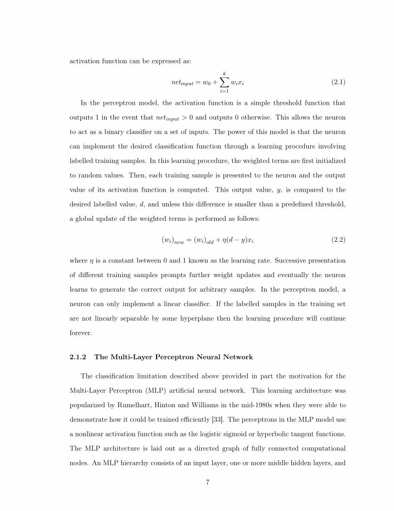
activation function can be expressed as:

netinput = w0 +

ki=1

wixi (2.1)

In the perceptron model, the activation function is a simple threshold function that

outputs 1 in the event that netinput > 0 and outputs 0 otherwise. This allows the neuron

to act as a binary classifier on a set of inputs. The power of this model is that the neuron

can implement the desired classification function through a learning procedure involving

labelled training samples. In this learning procedure, the weighted terms are first initialized

to random values. Then, each training sample is presented to the neuron and the output

value of its activation function is computed. This output value, y, is compared to the

desired labelled value, d, and unless this difference is smaller than a predefined threshold,

a global update of the weighted terms is performed as follows:

(wi)new = (wi)old + η(d− y)xi (2.2)

where η is a constant between 0 and 1 known as the learning rate. Successive presentation

of different training samples prompts further weight updates and eventually the neuron

learns to generate the correct output for arbitrary samples. In the perceptron model, a

neuron can only implement a linear classifier. If the labelled samples in the training set

are not linearly separable by some hyperplane then the learning procedure will continue

forever.

2.1.2 The Multi-Layer Perceptron Neural Network

The classification limitation described above provided in part the motivation for the

Multi-Layer Perceptron (MLP) artificial neural network. This learning architecture was

popularized by Rumelhart, Hinton and Williams in the mid-1980s when they were able to

demonstrate how it could be trained efficiently [33]. The perceptrons in the MLP model use

a nonlinear activation function such as the logistic sigmoid or hyperbolic tangent functions.

The MLP architecture is laid out as a directed graph of fully connected computational

nodes. An MLP hierarchy consists of an input layer, one or more middle hidden layers, and

7

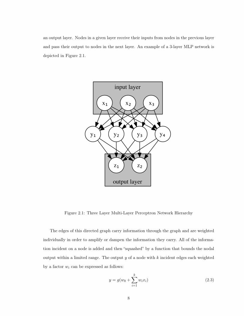
an output layer. Nodes in a given layer receive their inputs from nodes in the previous layer

and pass their output to nodes in the next layer. An example of a 3-layer MLP network is

depicted in Figure 2.1.

input layer

output layer

x₂

y₁ y₂ y₃ y₄

x₁ x₃

z₂z₁

Figure 2.1: Three Layer Multi-Layer Perceptron Network Hierarchy

The edges of this directed graph carry information through the graph and are weighted

individually in order to amplify or dampen the information they carry. All of the informa-

tion incident on a node is added and then “squashed” by a function that bounds the nodal

output within a limited range. The output y of a node with k incident edges each weighted

by a factor wi can be expressed as follows:

y = g(w0 +k

i=1

wixi) (2.3)

8

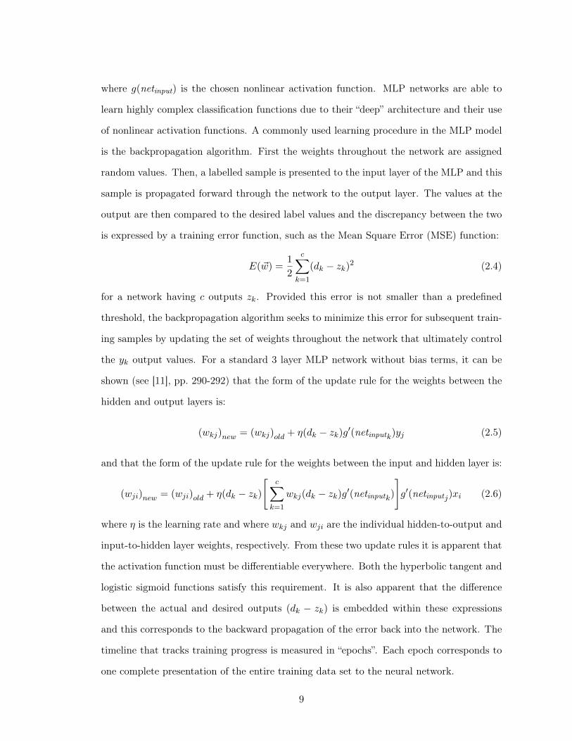
where g(netinput) is the chosen nonlinear activation function. MLP networks are able to

learn highly complex classification functions due to their “deep” architecture and their use

of nonlinear activation functions. A commonly used learning procedure in the MLP model

is the backpropagation algorithm. First the weights throughout the network are assigned

random values. Then, a labelled sample is presented to the input layer of the MLP and this

sample is propagated forward through the network to the output layer. The values at the

output are then compared to the desired label values and the discrepancy between the two

is expressed by a training error function, such as the Mean Square Error (MSE) function:

E(w⃗) =1

2

ck=1

(dk − zk)2 (2.4)

for a network having c outputs zk. Provided this error is not smaller than a predefined

threshold, the backpropagation algorithm seeks to minimize this error for subsequent train-

ing samples by updating the set of weights throughout the network that ultimately control

the yk output values. For a standard 3 layer MLP network without bias terms, it can be

shown (see [11], pp. 290-292) that the form of the update rule for the weights between the

hidden and output layers is:

(wkj)new = (wkj)old + η(dk − zk)g′(netinputk)yj (2.5)

and that the form of the update rule for the weights between the input and hidden layer is:

(wji)new = (wji)old + η(dk − zk)

c

k=1

wkj(dk − zk)g′(netinputk)

g′(netinputj)xi (2.6)

where η is the learning rate and where wkj and wji are the individual hidden-to-output and

input-to-hidden layer weights, respectively. From these two update rules it is apparent that

the activation function must be differentiable everywhere. Both the hyperbolic tangent and

logistic sigmoid functions satisfy this requirement. It is also apparent that the difference

between the actual and desired outputs (dk − zk) is embedded within these expressions

and this corresponds to the backward propagation of the error back into the network. The

timeline that tracks training progress is measured in “epochs”. Each epoch corresponds to

one complete presentation of the entire training data set to the neural network.

9

2.1.3 Artificial Neural Network Training Considerations

The backpropagation algorithm is commonly carried out in one of two training modes:

stochastic and batch. In stochastic training mode, the weight updates are calculated and

applied after the presentation of each training sample to the MLP network. In batch training

mode, the weight updates required for every sample are accumulated over an epoch and

stored, but the actual update is only applied after the full set (or some subset) of training

samples has been presented to the network. Batch training is usually considered the slower

of the two modes especially in cases where many of the training samples are very similar

or identical to each other.

The whole training procedure can be seen as trying to find a minimum point within a

highly-dimensional error function space. The dimension of this space is equal to the number

of weight parameters in the neural network. The backpropagation algorithm is a gradient

descent algorithm that will find a local minimum in this space. The learning rate η controls

the magnitude of weight updates. In some cases, it is a fixed constant throughout the

training procedure, in other cases it is varied according to some learning rate schedule (e.g.

after n epochs, the learning rate is decreased by some factor k, where 0 < k < 1). The

value of η is nevertheless crucial to convergence of the training algorithm. If it is too small,

weights will change slowly and many epochs of training will be required. If it is too large,

weights might oscillate wildly and the algorithm will never settle within a local minimum.

2.2 Error-Correcting Codes

A common problem encountered in telecommunications and in the transcription of digi-

tal information onto physical media is that data sent or written is not what was actually

intended. In a telecommunications context, noise or interference in the communication

channel can cause errors in the transmission. In the digital transcription context, physi-

cal defects in the media can cause the wrong information to be written. Error-Correcting

Codes (ECC) are a method of dealing with these realities. The premise of this method is

to come up with a scheme to encode the information that is to be transmitted or written

10

in such a way that the receiver or reader can automatically detect and correct errors in the

data. This leads to a need for increased logic and time required for encoding and decoding

data but this is usually outweighed by the error correcting benefits.

2.2.1 Linear Binary Error-Correcting Codes

A linear binary ECC, denoted as [N,K,D] relies on a codebook C consisting of a set

of 2K codewords. Each codeword is a binary string of length N . The set of codewords

in C must satisfy the property that any two codewords in the codebook must differ in

bit values in at least D positions. D is referred to as the Hamming distance. For the

code to correct E possible errors in a transmitted symbol of length N , D must be at least

2E + 1. For example, a [7, 4, 3] code consists of a codebook filled with 16 7-bit codewords.

The transmitter interested in sending 4-bit messages across a noisy channel would encode

each message by the appropriate 7-bit codeword from the codebook. In the event that one

of the seven bits was flipped during transmission, the receiver would immediately realize

it (as the received codeword would not appear within the codebook), and would be able

to deduce which codeword was intended. This deduction procedure involves finding the

closest legal codeword to the message received. The underlying assumption here is that the

characteristics of the transmission channel are well known and, in this case, the possibility

of two or more bits being flipped simultaneously is remote. Even with this assumption in

mind, it is worth noting that the [7, 4, 3] code can even detect double bit errors but it is

not able to reliably correct them.

2.2.2 Hard Decoding vs Soft Decoding

It is useful to consider a hypothetical communications channel over which a binary ‘0’ is

transmitted as −1.0 Volts and a binary ‘1’ is transmitted as +1.0 Volts. The receiver of a 4-

bit codeword sent across this channel must also contend with the analog to digital conversion

of this signal and ECCs play an important role in this step. If the receiver were to measure

the signal voltages of an incoming codeword signal as, say, (−0.1, 0.1, 0.9,−0.9), then there

11

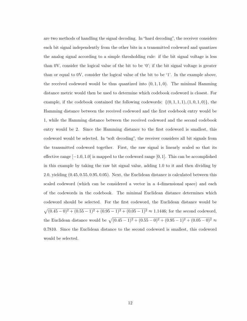
are two methods of handling the signal decoding. In “hard decoding”, the receiver considers

each bit signal independently from the other bits in a transmitted codeword and quantizes

the analog signal according to a simple thresholding rule: if the bit signal voltage is less

than 0V, consider the logical value of the bit to be ‘0’; if the bit signal voltage is greater

than or equal to 0V, consider the logical value of the bit to be ‘1’. In the example above,

the received codeword would be thus quantized into (0, 1, 1, 0). The minimal Hamming

distance metric would then be used to determine which codebook codeword is closest. For

example, if the codebook contained the following codewords: {(0, 1, 1, 1), (1, 0, 1, 0)}, the

Hamming distance between the received codeword and the first codebook entry would be

1, while the Hamming distance between the received codeword and the second codebook

entry would be 2. Since the Hamming distance to the first codeword is smallest, this

codeword would be selected. In “soft decoding”, the receiver considers all bit signals from

the transmitted codeword together. First, the raw signal is linearly scaled so that its

effective range [−1.0, 1.0] is mapped to the codeword range [0, 1]. This can be accomplished

in this example by taking the raw bit signal value, adding 1.0 to it and then dividing by

2.0, yielding (0.45, 0.55, 0.95, 0.05). Next, the Euclidean distance is calculated between this

scaled codeword (which can be considered a vector in a 4-dimensional space) and each

of the codewords in the codebook. The minimal Euclidean distance determines which

codeword should be selected. For the first codeword, the Euclidean distance would be(0.45− 0)2 + (0.55− 1)2 + (0.95− 1)2 + (0.05− 1)2 ≈ 1.1446; for the second codeword,

the Euclidean distance would be

(0.45− 1)2 + (0.55− 0)2 + (0.95− 1)2 + (0.05− 0)2 ≈

0.7810. Since the Euclidean distance to the second codeword is smallest, this codeword

would be selected.

12

CHAPTER 3. CONVOLUTIONAL NEURAL NETWORKS

3.1 Motivation

MLP networks are able to learn complex functions that allow classification of input data

into one of multiple classes. While this is a quite useful and powerful property, practitioners

that would like to use this functionality within a real-world pattern recognition system still

need to contend with the fact that MLP networks were conceived to be trained by and

operated on extracted features from raw input patterns (e.g. sound, audio or video). In

addition, a fully-connected network grows very quickly as neurons are added to the various

layers and this can make it computationally slow for some real-world problems.

The Convolutional Neural Network (CNN) is a refinement of the generic MLP neural

network that is partly inspired by the way the animal visual system is arranged. In the

1960’s, Hubel and Wiesel discovered two types of neuronal cells within the cat’s primary

visual cortex: simple cells and complex cells [19]. These cells respond to different kinds of

stimuli applied to their receptive fields (very specific areas on the retinal surface). Simple

cells fire when the pattern within the receptive field contains a contrasting line or edge (e.g.

white line against a black background or a dark line against a white background) but are

very sensitive to the orientation and position of this feature within the receptive field. Any

small change in orientation or position of the feature within the receptive field leads to a

reduction in simple cell firing. Complex cells, on the other hand, fire when the pattern

within the receptive field contains a line or edge that is oriented in a specific direction and

will still fire regardless of the feature’s position within the receptive field. Complex cells thus

exhibit a kind of invariance with respect to position. A complex cell receives its input from

several simple cells and complex cells pass their outputs to higher-level complex cells. More

13

complex features present in the receptive field, such as corners or angles, trigger higher-

level complex cells. Higher complex cells in the hierarchy are sensitive only to increasingly

elaborate features and display an incredible degree of invariance to feature illumination,

position, size or rotation.

The CNN appears to have been discovered independently by both Fukushima in the

1980s who referred to it as the Neocognitron [13] and by LeCun who was responsible for

showing how such an architecture could be trained in a completely supervised manner [24].

The CNN incorporates a hierarchical structure such that elementary features of a training

pattern are detected at the lower levels and more complex features are detected at the

higher levels. As in the biological case of neurons in the visual cortex, the goal of this

organization is to make the higher level feature detectors more robust to slight variations

in the input pattern.

3.2 CNN Applications

CNNs have been used and continue to be used in state-of-the-art applications ranging

from the recognition of characters written in different scripts [25] [34] [1] and objects [26] to

the detection of speech [36], faces [14], license plates [5], pedestrians [38] to the prediction

of player moves in the classic board game Go [37]. A survey of significant CNN applications

in vision was recently conducted [27].

Traditionally CNNs have been trained on conventional computer CPUs. It was not

uncommon to hear about training sessions running for weeks or months in the 1990s, days

or weeks in the early 2000s and hours or days in the mid to late 2000s. In the late 2000s,

the processing power of Graphical Processing Units for general purpose computing became

easier to exploit and the first artificial neural network training implementations were devel-

oped [6] [35]. These new implementations, while still in their infancy, will likely permit the

design of deeper networks with greater capacities, increased performance and significantly

decreased training times.

14

3.3 CNN Architecture

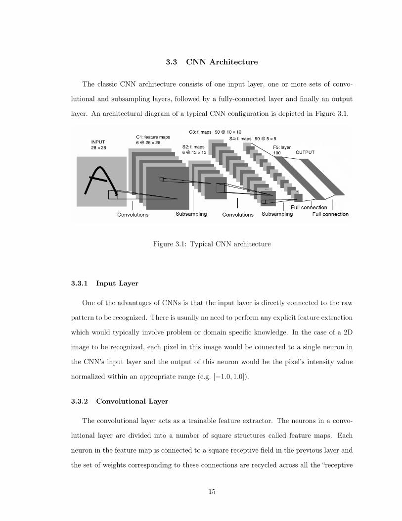
The classic CNN architecture consists of one input layer, one or more sets of convo-

lutional and subsampling layers, followed by a fully-connected layer and finally an output

layer. An architectural diagram of a typical CNN configuration is depicted in Figure 3.1.

Figure 3.1: Typical CNN architecture

3.3.1 Input Layer

One of the advantages of CNNs is that the input layer is directly connected to the raw

pattern to be recognized. There is usually no need to perform any explicit feature extraction

which would typically involve problem or domain specific knowledge. In the case of a 2D

image to be recognized, each pixel in this image would be connected to a single neuron in

the CNN’s input layer and the output of this neuron would be the pixel’s intensity value

normalized within an appropriate range (e.g. [−1.0, 1.0]).

3.3.2 Convolutional Layer

The convolutional layer acts as a trainable feature extractor. The neurons in a convo-

lutional layer are divided into a number of square structures called feature maps. Each

neuron in the feature map is connected to a square receptive field in the previous layer and

the set of weights corresponding to these connections are recycled across all the “receptive

15

field”-to-“convolutional layer neuron” connections in a given feature map. The selection of

receptive field zones is made in a systematic way, in much the same way as a filtering kernel

would be applied to or convolved over an entire image in an image processing context.

An example might better illustrate this arrangement. Assume the input layer consists of

32× 32 neurons n0,x,y (where both indices x and y lie within [0, 31]) and the next layer is a

convolutional layer consisting of 2 feature maps, each containing 28× 28 neurons n1,a,b and

n2,a,b respectively (where the indices lie within [0, 27]), and the receptive field (i.e. filtering

kernel) size is 5 × 5. The first feature map is assigned a set of 25 trainable weights w1,i,j

(where both indices i and j lie within [0, 4]) and a trainable bias b1. Similarly, the second

feature map is assigned a different set of 25 trainable weights w2,i,j (where both indices i

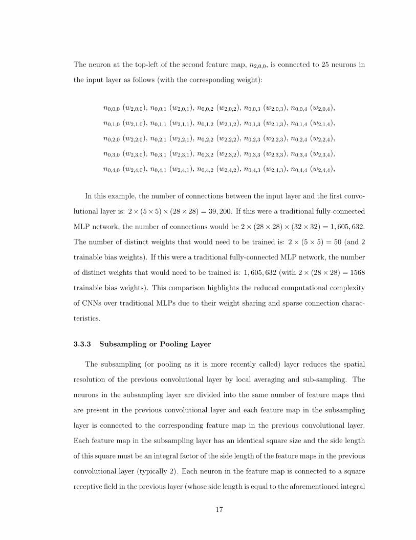
and j lie within [0, 4]) and a trainable bias b2. The neuron at the top-left of the first feature

map, n1,0,0, is connected to 25 neurons in the input layer as follows (with the corresponding

weight):

n0,0,0 (w1,0,0), n0,0,1 (w1,0,1), n0,0,2 (w1,0,2), n0,0,3 (w1,0,3), n0,0,4 (w1,0,4),

n0,1,0 (w1,1,0), n0,1,1 (w1,1,1), n0,1,2 (w1,1,2), n0,1,3 (w1,1,3), n0,1,4 (w1,1,4),

n0,2,0 (w1,2,0), n0,2,1 (w1,2,1), n0,2,2 (w1,2,2), n0,2,3 (w1,2,3), n0,2,4 (w1,2,4),

n0,3,0 (w1,3,0), n0,3,1 (w1,3,1), n0,3,2 (w1,3,2), n0,3,3 (w1,3,3), n0,3,4 (w1,3,4),

n0,4,0 (w1,4,0), n0,4,1 (w1,4,1), n0,4,2 (w1,4,2), n0,4,3 (w1,4,3), n0,4,4 (w1,4,4),

The next neuron of the top row of the first feature map, n1,0,1, is connected to 25 neurons

in the input layer as follows (with the corresponding weight):

n0,0,1 (w1,0,0), n0,0,2 (w1,0,1), n0,0,3 (w1,0,2), n0,0,4 (w1,0,3), n0,0,5 (w1,0,4),

n0,1,1 (w1,1,0), n0,1,2 (w1,1,1), n0,1,3 (w1,1,2), n0,1,4 (w1,1,3), n0,1,5 (w1,1,4),

n0,2,1 (w1,2,0), n0,2,2 (w1,2,1), n0,2,3 (w1,2,2), n0,2,4 (w1,2,3), n0,2,5 (w1,2,4),

n0,3,1 (w1,3,0), n0,3,2 (w1,3,1), n0,3,3 (w1,3,2), n0,3,4 (w1,3,3), n0,3,5 (w1,3,4),

n0,4,1 (w1,4,0), n0,4,2 (w1,4,1), n0,4,3 (w1,4,2), n0,4,4 (w1,4,3), n0,4,5 (w1,4,4),

16

The neuron at the top-left of the second feature map, n2,0,0, is connected to 25 neurons in

the input layer as follows (with the corresponding weight):

n0,0,0 (w2,0,0), n0,0,1 (w2,0,1), n0,0,2 (w2,0,2), n0,0,3 (w2,0,3), n0,0,4 (w2,0,4),

n0,1,0 (w2,1,0), n0,1,1 (w2,1,1), n0,1,2 (w2,1,2), n0,1,3 (w2,1,3), n0,1,4 (w2,1,4),

n0,2,0 (w2,2,0), n0,2,1 (w2,2,1), n0,2,2 (w2,2,2), n0,2,3 (w2,2,3), n0,2,4 (w2,2,4),

n0,3,0 (w2,3,0), n0,3,1 (w2,3,1), n0,3,2 (w2,3,2), n0,3,3 (w2,3,3), n0,3,4 (w2,3,4),

n0,4,0 (w2,4,0), n0,4,1 (w2,4,1), n0,4,2 (w2,4,2), n0,4,3 (w2,4,3), n0,4,4 (w2,4,4),

In this example, the number of connections between the input layer and the first convo-

lutional layer is: 2× (5× 5)× (28× 28) = 39, 200. If this were a traditional fully-connected

MLP network, the number of connections would be 2× (28× 28)× (32× 32) = 1, 605, 632.

The number of distinct weights that would need to be trained is: 2 × (5 × 5) = 50 (and 2

trainable bias weights). If this were a traditional fully-connected MLP network, the number

of distinct weights that would need to be trained is: 1, 605, 632 (with 2× (28× 28) = 1568

trainable bias weights). This comparison highlights the reduced computational complexity

of CNNs over traditional MLPs due to their weight sharing and sparse connection charac-

teristics.

3.3.3 Subsampling or Pooling Layer

The subsampling (or pooling as it is more recently called) layer reduces the spatial

resolution of the previous convolutional layer by local averaging and sub-sampling. The

neurons in the subsampling layer are divided into the same number of feature maps that

are present in the previous convolutional layer and each feature map in the subsampling

layer is connected to the corresponding feature map in the previous convolutional layer.

Each feature map in the subsampling layer has an identical square size and the side length

of this square must be an integral factor of the side length of the feature maps in the previous

convolutional layer (typically 2). Each neuron in the feature map is connected to a square

receptive field in the previous layer (whose side length is equal to the aforementioned integral

17

factor), however, unlike the case of receptive fields used by convolutional areas which are

overlapping, these receptive fields are not. The outputs of the neurons comprising the

receptive field are either averaged together or the maximum value is chosen. The non-

overlapping nature of these fields leads to the subsampling effect that this layer is named

for.

There are several ways that the subsampling layer is used in practice. In many imple-

mentations, a constant activation function is used in this layer instead of a sigmoid. In such

implementations, the equivalent effect of this layer is achieved through the use of a step

size within the corresponding convolutional layer. This is more computationally efficient

since it avoids the needless computation of neuron output values in the convolutional layer

that would otherwise be discarded by the subsampling layer and reduces the architectural

complexity of the overall CNN.

3.3.4 Fully-Connected Layer

The fully-connected layer acts as generic classifier. Every neuron in this layer is connected

to every neuron in the previous layer. The size (capacity) of this layer has a significant effect

on the ability of the network to generalize in the case of test patterns and must usually be

determined experimentally on a validation set (typically a small subset of the training set

which has been set aside and not used for training the CNN).

3.3.5 Output Layer

The output layer is usually fully-connected to the previous fully-connected layer. The

CNN’s output vector is constructed by taking the output of each neuron in turn from this

layer. The interpretation of this output vector is determined by the scheme used to code

it. Some alternative schemes are presented below.

18

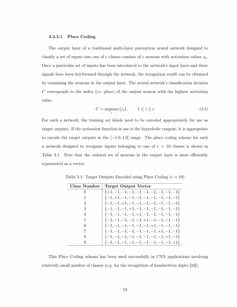
3.3.5.1 Place Coding

The output layer of a traditional multi-layer perceptron neural network designed to

classify a set of inputs into one of c classes consists of c neurons with activation values zk.

Once a particular set of inputs has been introduced to the network’s input layer and these

signals have been fed-forward through the network, the recognition result can be obtained

by examining the neurons in the output layer. The neural network’s classification decision

C corresponds to the index (i.e. place) of the output neuron with the highest activation

value:

C = argmaxi{zi} , 1 ≤ i ≤ c (3.1)

For such a network, the training set labels need to be encoded appropriately for use as

target outputs. If the activation function in use is the hyperbolic tangent, it is appropriate

to encode the target outputs in the [−1.0, 1.0] range. The place coding scheme for such

a network designed to recognize inputs belonging to one of c = 10 classes is shown in

Table 3.1. Note that the ordered set of neurons in the output layer is most efficiently

represented as a vector.

Table 3.1: Target Outputs Encoded using Place Coding (c = 10)

Class Number Target Output Vector0 {+1,−1,−1,−1,−1,−1,−1,−1,−1,−1}1 {−1,+1,−1,−1,−1,−1,−1,−1,−1,−1}2 {−1,−1,+1,−1,−1,−1,−1,−1,−1,−1}3 {−1,−1,−1,+1,−1,−1,−1,−1,−1,−1}4 {−1,−1,−1,−1,+1,−1,−1,−1,−1,−1}5 {−1,−1,−1,−1,−1,+1,−1,−1,−1,−1}6 {−1,−1,−1,−1,−1,−1,+1,−1,−1,−1}7 {−1,−1,−1,−1,−1,−1,−1,+1,−1,−1}8 {−1,−1,−1,−1,−1,−1,−1,−1,+1,−1}9 {−1,−1,−1,−1,−1,−1,−1,−1,−1,+1}

This Place Coding scheme has been used successfully in CNN applications involving

relatively small number of classes (e.g. for the recognition of handwritten digits [34]).

19

3.3.5.2 Distributed Coding

Place Coding is certainly not the only possibility for target output vector encoding.

The use of Place Coding is discouraged for problems involving a large number of classes

because it is difficult for the neural network’s sigmoidal units to keep all but one of the

outputs at their minimal values [25]. Distributed codes involve encoding each class label

by a codeword and training the network using the set of class codewords as target output

vectors. Some suggestions made in Lecun et al’s 1998 paper include random coding, error-

correcting coding and a stylized image coding scheme [25]. In random coding, each element

of the output codeword vector (−1 or +1) is chosen randomly with equal probability and the

set of generated codewords is verified to ensure there are no duplicates contained therein.

In error-correcting output coding, the set of codewords is chosen according to an error-

correcting code. The stylized image coding scheme is the scheme actually used for the

experiments described in LeCun’s paper and it consists of 96 codewords (representing all

the characters of the printable ASCII set) of length 84. When these codewords are arranged

as 7 × 12 bitmaps, a stylized image of the corresponding class is clearly discernible. The

advantage of using this type of distributed code is that similar character classes are assigned

similar output codes (e.g. the ‘1’ and ‘l’ classes).

The neural network’s classification decision C corresponds to the codebook index i of

the codeword vector d⃗(i) whose Euclidean distance is closest to the output layer’s output

vector z⃗ (the magnitudes of d⃗i and z⃗ are both k):

C = argmini

k

n=1

zn − d

(i)n

2 , 1 ≤ i ≤ c (3.2)

3.4 CNN Recognition Confidence and Rejection Schemes

In many pattern recognition tasks, it can be very helpful to have the classifier return a

confidence value along with its classification choice. The confidence metric tries to commu-

nicate the classifier’s level of certainty at the time it made its classification decision. In

some contexts, the classifier is given a rejection option that it may exercise in the event

20

that it is truly unsure or cannot make a decision. An example of such a context is the

automated mail sorting machines at a postal service facility. In the event that the classifier

is unsure about its ability to correctly recognize the destination address on an envelope, it

can reject the sample which will cause it to be routed to a human postal worker for manual

processing.

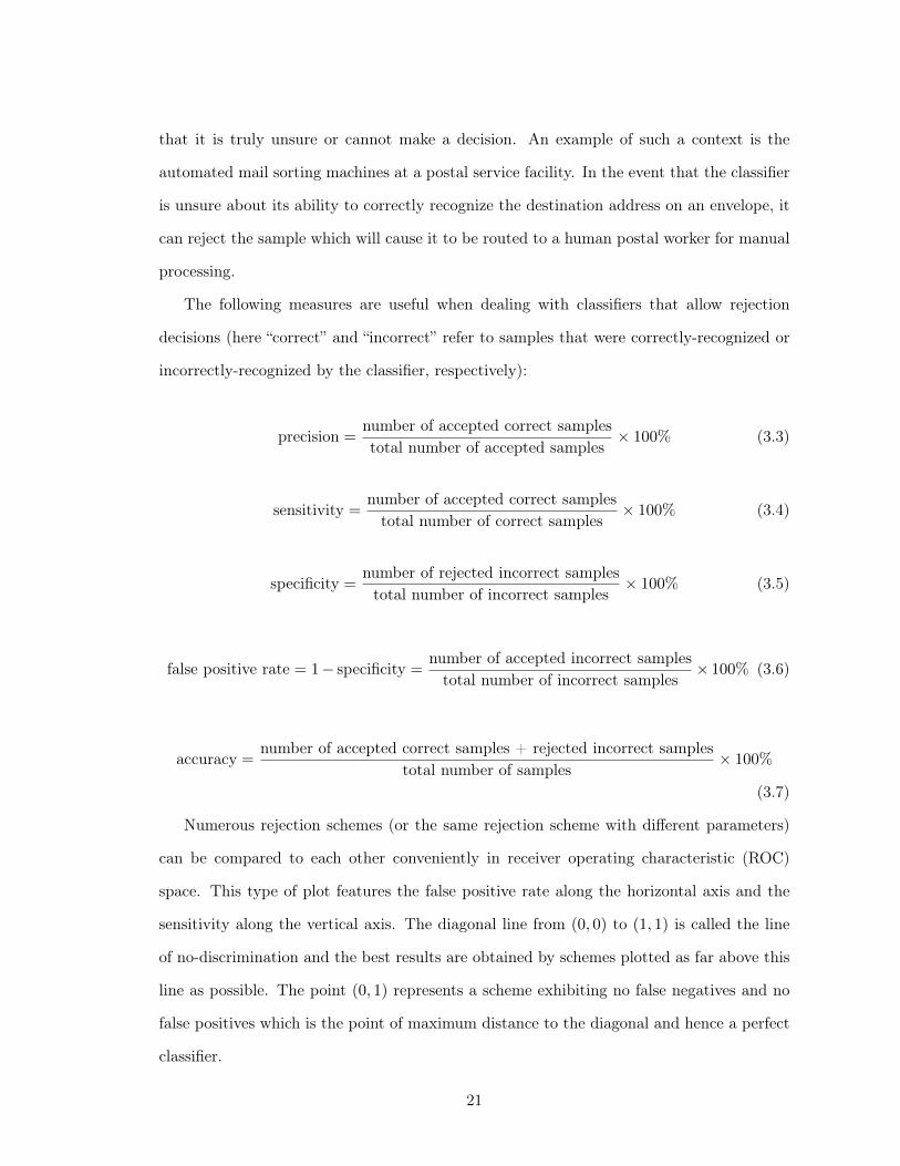
The following measures are useful when dealing with classifiers that allow rejection

decisions (here “correct” and “incorrect” refer to samples that were correctly-recognized or

incorrectly-recognized by the classifier, respectively):

precision =number of accepted correct samplestotal number of accepted samples

× 100% (3.3)

sensitivity =number of accepted correct samples

total number of correct samples× 100% (3.4)

specificity =number of rejected incorrect samples

total number of incorrect samples× 100% (3.5)

false positive rate = 1− specificity =number of accepted incorrect samples

total number of incorrect samples× 100% (3.6)

accuracy =number of accepted correct samples + rejected incorrect samples

total number of samples× 100%

(3.7)

Numerous rejection schemes (or the same rejection scheme with different parameters)

can be compared to each other conveniently in receiver operating characteristic (ROC)

space. This type of plot features the false positive rate along the horizontal axis and the

sensitivity along the vertical axis. The diagonal line from (0, 0) to (1, 1) is called the line

of no-discrimination and the best results are obtained by schemes plotted as far above this

line as possible. The point (0, 1) represents a scheme exhibiting no false negatives and no

false positives which is the point of maximum distance to the diagonal and hence a perfect

classifier.

21

The most straight-forward CNN confidence metric is based on thresholds. In the case of

a CNN using Place Coding, once the classification decision has been made (i.e. the output

neuron with the highest activation value has been determined), the output value of the

corresponding output neuron is compared to some constant threshold value. If this output

value is less than the threshold, the sample is rejected, otherwise it is accepted. In the case

of a CNN using Distributed Coding, the minimal Euclidean distance to a valid codeword can

be compared to some constant threshold value. If this distance is larger than the threshold,

the sample is rejected, otherwise it is accepted. Another scheme involves considering the

difference between the top two candidate classes and rejecting the sample if this difference

is smaller than some constant threshold value [25].

3.5 CNN Hyper-Parameters and System Attributes

Artificial neural networks and CNNs in particular are fully specified by a set of hyper-

parameters and system attributes. The values of these parameters are usually determined

experimentally as they vary considerably from one problem to the next. In order to report

CNN experimental results in a reproducible fashion, the complete set of hyper-parameter

and system attribute values used should be specified. Unfortunately, published studies

involving CNNs often fail to disclose all these details. A fairly complete list of these system

attributes known to have an effect on CNN training characteristics and recognition perfor-

mance has been compiled below:

• the number of convolutional layers, subsampling/pooling layers, fully-connected layers

used and the order in which they are arranged

• the number and sizes of feature maps and kernels used in the convolutional and

subsampling/pooling layers

• the nature of the activation functions used (i.e. the type of sigmoid and the value of

any constant coefficients used)

22

• the presence of an activation function after the subsampling/pooling layer and the

nature of this activation function if it is used

• the initial weight initialization scheme (i.e. same scheme for each CNN layer, nature

of the distribution from which random weights are selected)

• the learning rate used and whether it was fixed throughout training or varied according

to some schedule (which should also be described)

• the style of weight updating during training: error term accumulated and weights

updated over a batch of samples or after every single sample

• the use of artificially-created distorted images for training set augmentation and the

exact nature of the distortion scheme used

• the training stopping criterion (e.g. when error function reaches some arbitrary mini-

mum, when test error on a validation set reaches some minimum) and/or the number

of epochs that the CNN was trained for

• the choice of error function (e.g. mean-squared, Minkowski-R, cross-entropy)

• the input normalization procedure (e.g. the chosen output range for the input layer

neurons)

• the output coding scheme employed

23

CHAPTER 4. IMPROVING CNN PERFORMANCE

In this thesis, a system-level approach to the basic Convolutional Neural Network

machine learning technique is taken. Two modifications to the basic model are proposed

and implemented, one at the CNN’s input and one at the CNN’s output: Recognition Input

Squinting and Error-Correcting Output Coding, respectively. This section introduces these

modifications and presents the motivation for their use.

4.1 Recognition Input Squinting

4.1.1 Motivation

The novel Recognition Input Squinting modification is grounded in four straight-forward

observations:

1. One of the characteristic strengths of the CNN is its invariance to small translational,

rotational or skewing in the input image.

2. A CNN is best trained with a large amount of training data. Since this data is typically

expensive to obtain, it has been suggested that an existing labelled training set can

be greatly extended by applying artificial distortions to each of the data samples.

There are several types of distortions that can be applied to an image that should

still render it recognizable. Affine transformations (e.g. translation with perhaps some

degree of scaling, rotation and sheering) [25] and elastic deformations [34] have been

suggested as suitable candidates. CNNs trained on these distorted data sets have

been consistently shown to generalize better on test set patterns than those that

have not [22]. More recent approaches to the problem of limited labelled training

24

data involve the use of unsupervised learning to train the lower layers of the CNN

and then supervised training to train the upper layers (e.g. [28]) but these methods

require large quantities of unlabelled training data.

3. CNNs were inspired by biology, specifically the hierarchical organization of neural

pathways within the animal visual cortex. Recent advances in automated vehicle

control by CNN [18] have also been inspired by biology in their use of stereo vision

and experiments have shown that significantly better results are obtained when two

cameras are used for obstacle avoidance rather than one.

4. Humans tend to go through a series of actions when they try to make sense of a visual

pattern they are not familiar with. These almost instinctual actions include:

(a) squinting one’s eyes

(b) tilting one’s neck to one side

(c) moving one’s head away from the pattern or closer to the pattern

(d) standing on one’s tippy toes or bending one’s knees in order to change the visual

angle of elevation

among other possibilities. In the event the visual pattern is printed on a physical

piece of paper, manual manipulations can be carried out, such as

(i) putting the paper under different illumination conditions

(ii) rotating the paper (similar to (b) above)

(iii) bringing the paper closer to the eye (similar to (c) above)

(iv) tilting the paper around the 3 dimensional perpendicular axes relative to the

eye’s gaze (similar to (d) above)

(v) crumpling or stretching the paper (similar to (a) above)

These actions are ordered roughly by the likelihood that a human would engage in

them for a routine visual recognition task from most likely to least likely.

25

The psychologist Gibson in the 1950s suggests that the brain makes use of “visual

motion” to aid in perception [15] and that it is actually the continuous series of visual

transformations (such as the ones described in observation #4 above) which constitutes the

visual stimulus that is in turn recognized [16]. Gibson makes reference to an optic array

that is perpetually refreshed with image stills from observed motion and claims that the

identification of the invariances within successive stills is the essence of visual perception

and recognition [17].

The premise behind Recognition Input Squinting is that the visual biological analogy for

CNNs is incomplete in that it does not account for the natural mechanical actions used by

animals that typically accompany ambiguous recognition tasks. Instead it relies on a single

frame of input to form a classification decision. With Recognition Input Squinting, the CNN

is augmented by an artificial optic array containing the pattern recognized as well as some

synthetic images, referred to as “squinted images”, that are designed to crudely simulate

the types of transformation mentioned above. The CNN then proceeds to recognize each

pattern in turn and the results of these recognitions are fed into a processor that makes a

final recognition decision.

The hypotheses, grounded in the observations above, are that:

1. certain distorted versions of a particular input image might have a better chance at

being recognized correctly than the original image

2. the classifier’s independent evaluation of various distorted versions of the same image

might serve as the basis for a measure of confidence in the recognition result of the

original image or provide a rejection criterion

The squinted images are produced according to the same procedures used to distort

training set images in order to augment the total number of training patterns. The proce-

dure used to generate the squinted images are described in the following section.

26

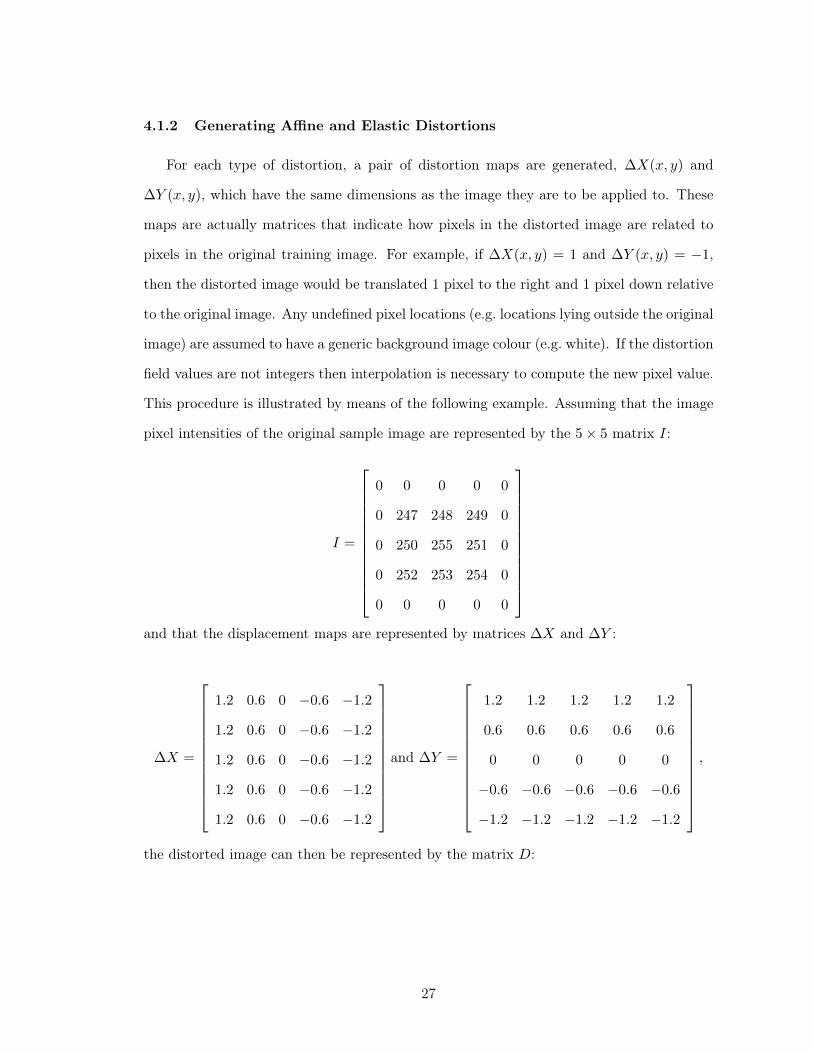
4.1.2 Generating Affine and Elastic Distortions

For each type of distortion, a pair of distortion maps are generated, ∆X(x, y) and

∆Y (x, y), which have the same dimensions as the image they are to be applied to. These

maps are actually matrices that indicate how pixels in the distorted image are related to

pixels in the original training image. For example, if ∆X(x, y) = 1 and ∆Y (x, y) = −1,

then the distorted image would be translated 1 pixel to the right and 1 pixel down relative

to the original image. Any undefined pixel locations (e.g. locations lying outside the original

image) are assumed to have a generic background image colour (e.g. white). If the distortion

field values are not integers then interpolation is necessary to compute the new pixel value.

This procedure is illustrated by means of the following example. Assuming that the image

pixel intensities of the original sample image are represented by the 5× 5 matrix I:

I =

0 0 0 0 0

0 247 248 249 0

0 250 255 251 0

0 252 253 254 0

0 0 0 0 0

and that the displacement maps are represented by matrices ∆X and ∆Y :

∆X =

1.2 0.6 0 −0.6 −1.2

1.2 0.6 0 −0.6 −1.2

1.2 0.6 0 −0.6 −1.2

1.2 0.6 0 −0.6 −1.2

1.2 0.6 0 −0.6 −1.2

and ∆Y =

1.2 1.2 1.2 1.2 1.2

0.6 0.6 0.6 0.6 0.6

0 0 0 0 0

−0.6 −0.6 −0.6 −0.6 −0.6

−1.2 −1.2 −1.2 −1.2 −1.2

,

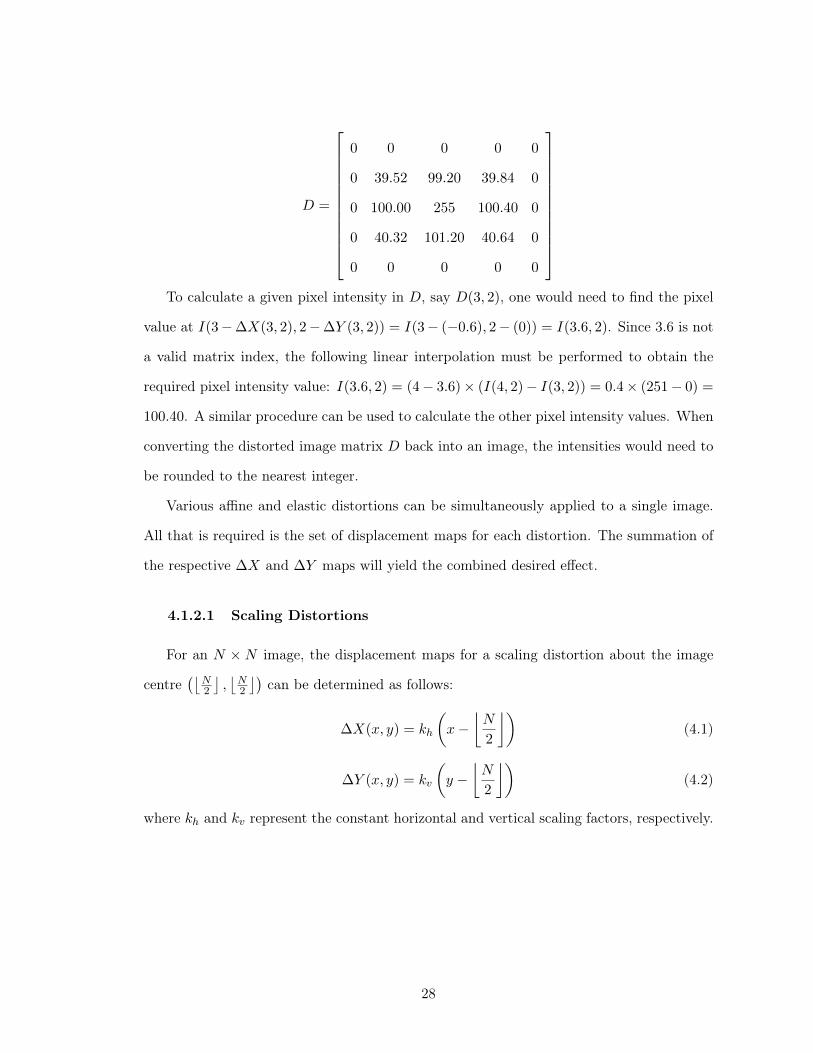
the distorted image can then be represented by the matrix D:

27

D =

0 0 0 0 0

0 39.52 99.20 39.84 0

0 100.00 255 100.40 0

0 40.32 101.20 40.64 0

0 0 0 0 0

To calculate a given pixel intensity in D, say D(3, 2), one would need to find the pixel

value at I(3−∆X(3, 2), 2−∆Y (3, 2)) = I(3− (−0.6), 2− (0)) = I(3.6, 2). Since 3.6 is not

a valid matrix index, the following linear interpolation must be performed to obtain the

required pixel intensity value: I(3.6, 2) = (4− 3.6)× (I(4, 2)− I(3, 2)) = 0.4× (251− 0) =

100.40. A similar procedure can be used to calculate the other pixel intensity values. When

converting the distorted image matrix D back into an image, the intensities would need to

be rounded to the nearest integer.

Various affine and elastic distortions can be simultaneously applied to a single image.

All that is required is the set of displacement maps for each distortion. The summation of

the respective ∆X and ∆Y maps will yield the combined desired effect.

4.1.2.1 Scaling Distortions

For an N × N image, the displacement maps for a scaling distortion about the image

centre

N2

,N2

can be determined as follows:

∆X(x, y) = kh

x−

N

2

(4.1)

∆Y (x, y) = kv

y −

N

2

(4.2)

where kh and kv represent the constant horizontal and vertical scaling factors, respectively.

28

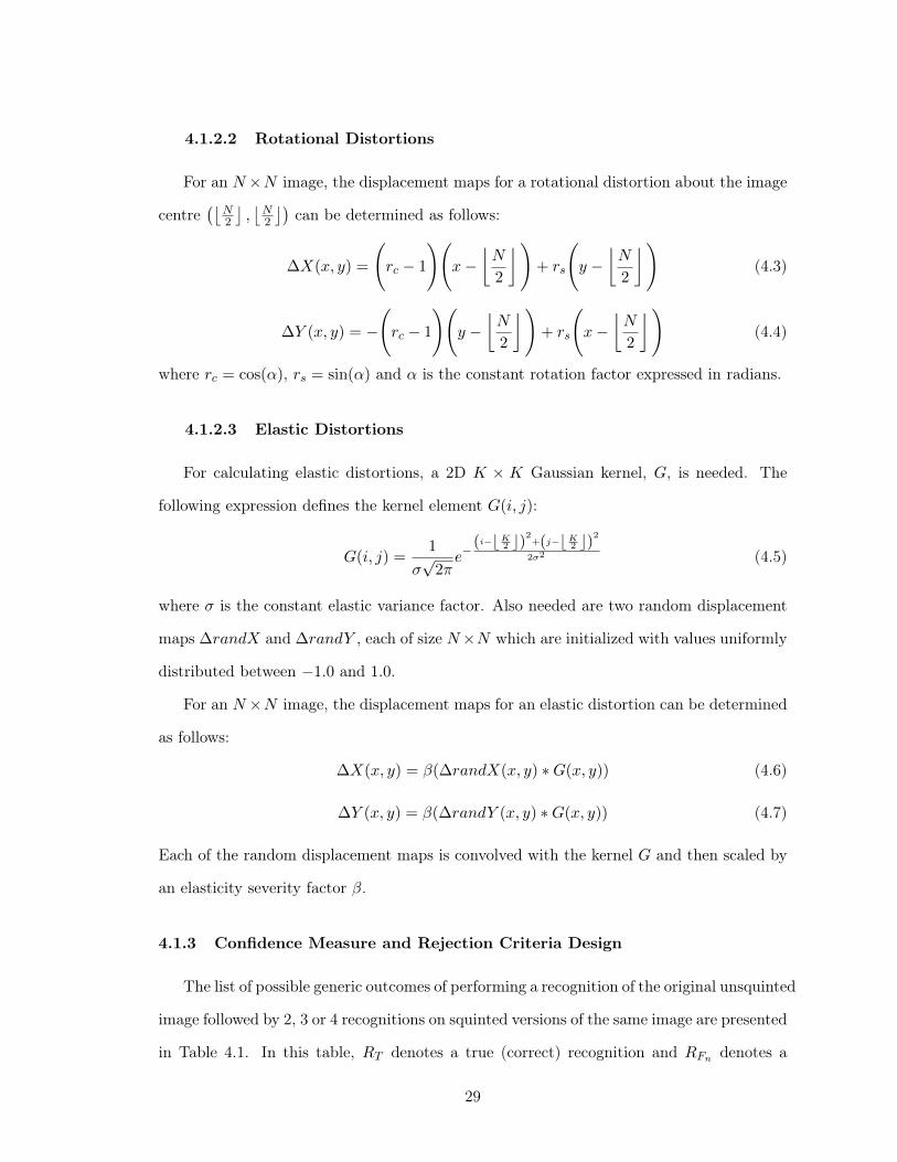
4.1.2.2 Rotational Distortions

For an N ×N image, the displacement maps for a rotational distortion about the image

centre

N2

,N2

can be determined as follows:

∆X(x, y) =

rc − 1

x−

N

2

+ rs

y −

N

2

(4.3)

∆Y (x, y) = −

rc − 1

y −

N

2

+ rs

x−

N

2

(4.4)

where rc = cos(α), rs = sin(α) and α is the constant rotation factor expressed in radians.

4.1.2.3 Elastic Distortions

For calculating elastic distortions, a 2D K × K Gaussian kernel, G, is needed. The

following expression defines the kernel element G(i, j):

G(i, j) =1

σ√2π

e−(i−⌊K2 ⌋)2+(j−⌊K2 ⌋)2

2σ2 (4.5)

where σ is the constant elastic variance factor. Also needed are two random displacement

maps ∆randX and ∆randY , each of size N×N which are initialized with values uniformly

distributed between −1.0 and 1.0.

For an N ×N image, the displacement maps for an elastic distortion can be determined

as follows:

∆X(x, y) = β(∆randX(x, y) ∗G(x, y)) (4.6)

∆Y (x, y) = β(∆randY (x, y) ∗G(x, y)) (4.7)

Each of the random displacement maps is convolved with the kernel G and then scaled by

an elasticity severity factor β.

4.1.3 Confidence Measure and Rejection Criteria Design

The list of possible generic outcomes of performing a recognition of the original unsquinted

image followed by 2, 3 or 4 recognitions on squinted versions of the same image are presented

in Table 4.1. In this table, RT denotes a true (correct) recognition and RFn denotes a

29

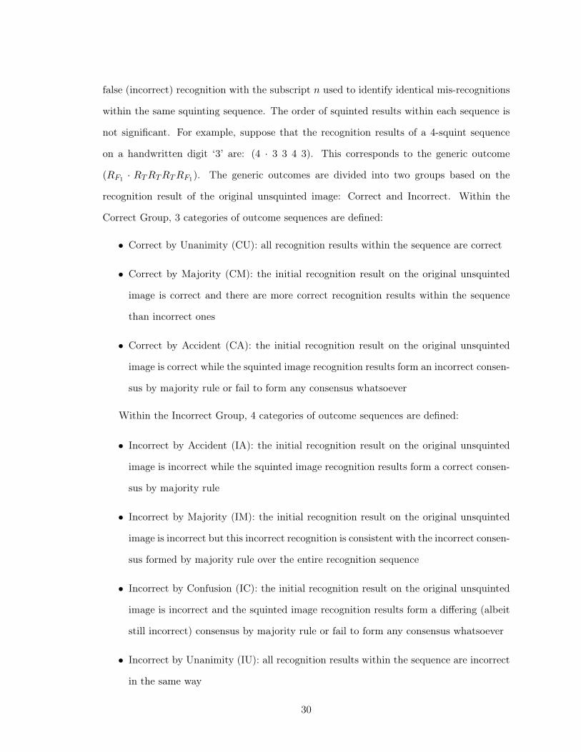
false (incorrect) recognition with the subscript n used to identify identical mis-recognitions

within the same squinting sequence. The order of squinted results within each sequence is

not significant. For example, suppose that the recognition results of a 4-squint sequence

on a handwritten digit ‘3’ are: (4 · 3 3 4 3). This corresponds to the generic outcome

(RF1 · RTRTRTRF1). The generic outcomes are divided into two groups based on the

recognition result of the original unsquinted image: Correct and Incorrect. Within the

Correct Group, 3 categories of outcome sequences are defined:

• Correct by Unanimity (CU): all recognition results within the sequence are correct

• Correct by Majority (CM): the initial recognition result on the original unsquinted

image is correct and there are more correct recognition results within the sequence

than incorrect ones

• Correct by Accident (CA): the initial recognition result on the original unsquinted

image is correct while the squinted image recognition results form an incorrect consen-

sus by majority rule or fail to form any consensus whatsoever

Within the Incorrect Group, 4 categories of outcome sequences are defined:

• Incorrect by Accident (IA): the initial recognition result on the original unsquinted

image is incorrect while the squinted image recognition results form a correct consen-

sus by majority rule

• Incorrect by Majority (IM): the initial recognition result on the original unsquinted

image is incorrect but this incorrect recognition is consistent with the incorrect consen-

sus formed by majority rule over the entire recognition sequence

• Incorrect by Confusion (IC): the initial recognition result on the original unsquinted

image is incorrect and the squinted image recognition results form a differing (albeit

still incorrect) consensus by majority rule or fail to form any consensus whatsoever

• Incorrect by Unanimity (IU): all recognition results within the sequence are incorrect

in the same way

30

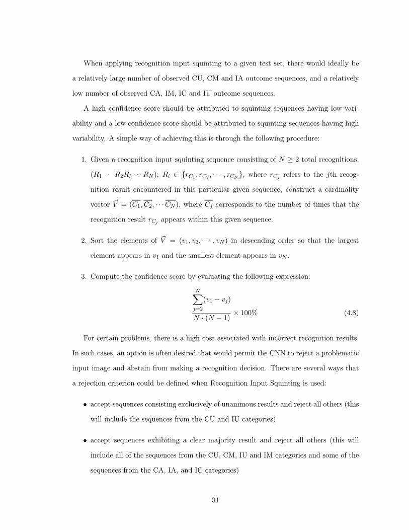
When applying recognition input squinting to a given test set, there would ideally be

a relatively large number of observed CU, CM and IA outcome sequences, and a relatively

low number of observed CA, IM, IC and IU outcome sequences.

A high confidence score should be attributed to squinting sequences having low vari-

ability and a low confidence score should be attributed to squinting sequences having high

variability. A simple way of achieving this is through the following procedure:

1. Given a recognition input squinting sequence consisting of N ≥ 2 total recognitions,

(R1 · R2R3 · · ·RN ); Ri ∈ {rC1 , rC2 , · · · , rCN}, where rCj refers to the jth recog-

nition result encountered in this particular given sequence, construct a cardinality

vector V⃗ = (C1, C2, · · ·CN ), where Cj corresponds to the number of times that the

recognition result rCj appears within this given sequence.

2. Sort the elements of V⃗ = (v1, v2, · · · , vN ) in descending order so that the largest

element appears in v1 and the smallest element appears in vN .

3. Compute the confidence score by evaluating the following expression:

Nj=2

(v1 − vj)

N · (N − 1)× 100% (4.8)

For certain problems, there is a high cost associated with incorrect recognition results.

In such cases, an option is often desired that would permit the CNN to reject a problematic

input image and abstain from making a recognition decision. There are several ways that

a rejection criterion could be defined when Recognition Input Squinting is used:

• accept sequences consisting exclusively of unanimous results and reject all others (this

will include the sequences from the CU and IU categories)

• accept sequences exhibiting a clear majority result and reject all others (this will

include all of the sequences from the CU, CM, IU and IM categories and some of the

sequences from the CA, IA, and IC categories)

31

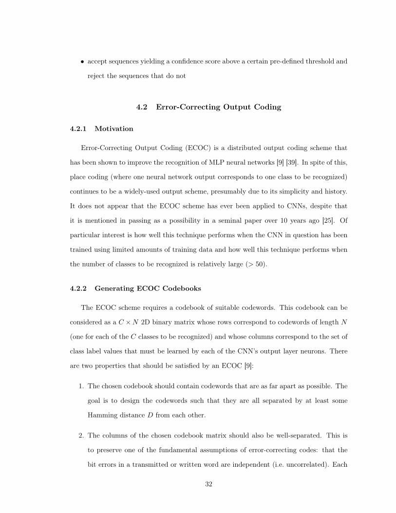
• accept sequences yielding a confidence score above a certain pre-defined threshold and

reject the sequences that do not

4.2 Error-Correcting Output Coding

4.2.1 Motivation

Error-Correcting Output Coding (ECOC) is a distributed output coding scheme that

has been shown to improve the recognition of MLP neural networks [9] [39]. In spite of this,

place coding (where one neural network output corresponds to one class to be recognized)

continues to be a widely-used output scheme, presumably due to its simplicity and history.

It does not appear that the ECOC scheme has ever been applied to CNNs, despite that

it is mentioned in passing as a possibility in a seminal paper over 10 years ago [25]. Of

particular interest is how well this technique performs when the CNN in question has been

trained using limited amounts of training data and how well this technique performs when

the number of classes to be recognized is relatively large (> 50).

4.2.2 Generating ECOC Codebooks

The ECOC scheme requires a codebook of suitable codewords. This codebook can be

considered as a C ×N 2D binary matrix whose rows correspond to codewords of length N

(one for each of the C classes to be recognized) and whose columns correspond to the set of

class label values that must be learned by each of the CNN’s output layer neurons. There

are two properties that should be satisfied by an ECOC [9]:

1. The chosen codebook should contain codewords that are as far apart as possible. The

goal is to design the codewords such that they are all separated by at least some

Hamming distance D from each other.

2. The columns of the chosen codebook matrix should also be well-separated. This is

to preserve one of the fundamental assumptions of error-correcting codes: that the

bit errors in a transmitted or written word are independent (i.e. uncorrelated). Each

32

Table 4.1: Generic Recognition Outcome Sequences for three squint counts

Category 2 Squints 3 Squints 4 SquintsCorrect by Unanimity (CU) RT ·RTRT RT ·RTRTRT RT ·RTRTRTRT

Correct by Majority RT ·RTRF1 RT ·RTRTRF1 RT ·RTRTRTRF1

RT ·RTRF1RF2 RT ·RTRTRF1RF1

RT ·RTRTRF1RF2

RT ·RTRF1RF2RF3

Correct by Accident (CA) RT ·RF1RF1 RT ·RTRF1RF1 RT ·RTRF1RF1RF1

RT ·RF1RF2 RT ·RF1RF1RF1 RT ·RTRF1RF1RF2

RT ·RF1RF1RF2 RT ·RF1RF1RF1RF1

RT ·RF1RF2RF3 RT ·RF1RF1RF1RF2

RT ·RF1RF1RF2RF2

RT ·RF1RF1RF2RF3

RT ·RF1RF2RF3RF4

Incorrect by Accident (IA) RF1 ·RTRT RF1 ·RTRTRT RF1 ·RTRTRTRT

RF1 ·RTRTRF2 RF1 ·RTRTRTRF1

RF1 ·RTRTRTRF2

RF1 ·RTRTRF2RF3

Incorrect by Majority (IM) RF1 ·RTRF1 RF1 ·RTRF1RF1 RF1 ·RTRTRF1RF1

RF1 ·RF1RF2 RF1 ·RTRF1RF2 RF1 ·RTRF1RF1RF1

RF1 ·RF1RF1RF2 RF1 ·RTRF1RF1RF2

RF1 ·RF1RF2RF3 RF1 ·RTRF1RF2RF3

RF1 ·RF1RF1RF1RF2

RF1 ·RF1RF1RF2RF2

RF1 ·RF1RF1RF2RF3

RF1 ·RF1RF2RF3RF4

Incorrect by Confusion (IC) RF1 ·RTRF2 RF1 ·RTRTRF1 RF1 ·RTRTRF1RF2

RF1 ·RF2RF2 RF1 ·RTRF2RF2 RF1 ·RTRTRF2RF2

RF1 ·RF2RF3 RF1 ·RTRF2RF3 RF1 ·RTRF1RF2RF2

RF1 ·RF1RF2RF2 RF1 ·RTRF2RF3RF4

RF1 ·RF2RF2RF2 RF1 ·RF1RF2RF2RF2

RF1 ·RF2RF2RF3 RF1 ·RF1RF2RF2RF3

RF1 ·RF2RF3RF4 RF1 ·RF1RF2RF3RF3

RF1 ·RF1RF2RF3RF4

RF1 ·RF2RF2RF2RF2

RF1 ·RF2RF2RF2RF3

RF1 ·RF2RF2RF3RF4

RF1 ·RF2RF3RF4RF5

Incorrect by Unanimity (IU) RF1 ·RF1RF1 RF1 ·RF1RF1RF1 RF1 ·RF1RF1RF1RF1

33

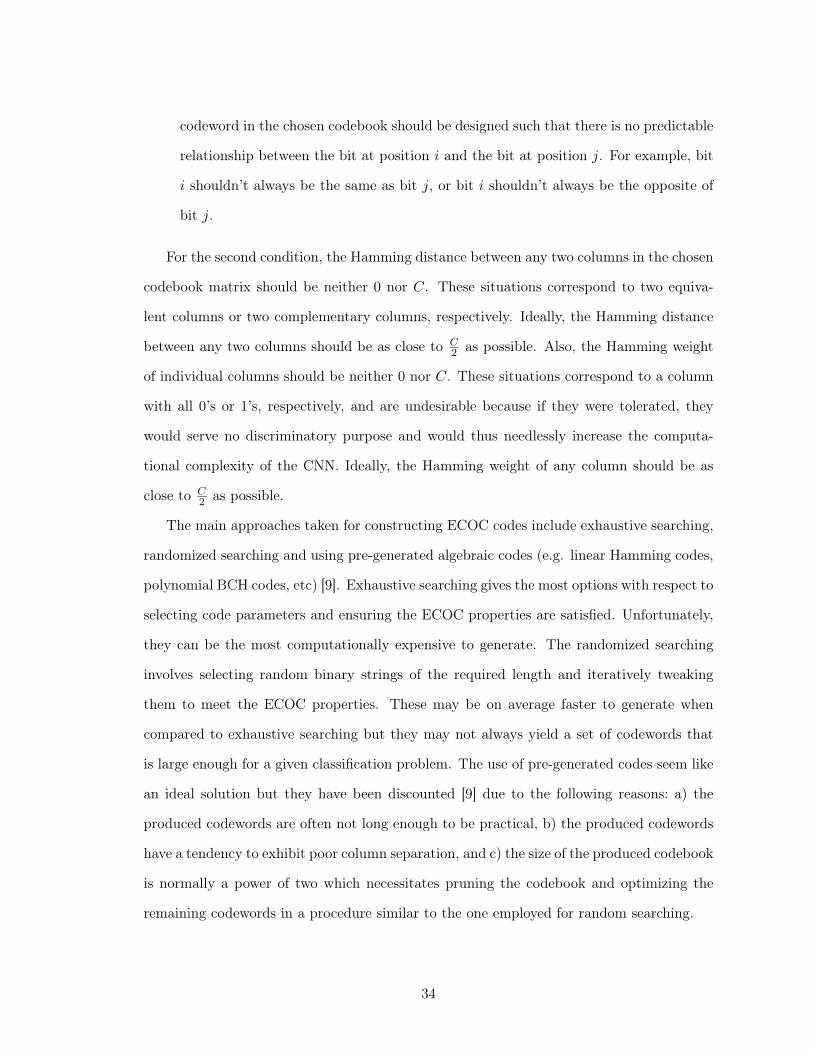
codeword in the chosen codebook should be designed such that there is no predictable

relationship between the bit at position i and the bit at position j. For example, bit

i shouldn’t always be the same as bit j, or bit i shouldn’t always be the opposite of

bit j.

For the second condition, the Hamming distance between any two columns in the chosen

codebook matrix should be neither 0 nor C. These situations correspond to two equiva-

lent columns or two complementary columns, respectively. Ideally, the Hamming distance

between any two columns should be as close to C2 as possible. Also, the Hamming weight

of individual columns should be neither 0 nor C. These situations correspond to a column

with all 0’s or 1’s, respectively, and are undesirable because if they were tolerated, they

would serve no discriminatory purpose and would thus needlessly increase the computa-

tional complexity of the CNN. Ideally, the Hamming weight of any column should be as

close to C2 as possible.

The main approaches taken for constructing ECOC codes include exhaustive searching,

randomized searching and using pre-generated algebraic codes (e.g. linear Hamming codes,

polynomial BCH codes, etc) [9]. Exhaustive searching gives the most options with respect to

selecting code parameters and ensuring the ECOC properties are satisfied. Unfortunately,

they can be the most computationally expensive to generate. The randomized searching

involves selecting random binary strings of the required length and iteratively tweaking

them to meet the ECOC properties. These may be on average faster to generate when

compared to exhaustive searching but they may not always yield a set of codewords that

is large enough for a given classification problem. The use of pre-generated codes seem like

an ideal solution but they have been discounted [9] due to the following reasons: a) the

produced codewords are often not long enough to be practical, b) the produced codewords

have a tendency to exhibit poor column separation, and c) the size of the produced codebook

is normally a power of two which necessitates pruning the codebook and optimizing the

remaining codewords in a procedure similar to the one employed for random searching.

34

4.2.2.1 Generation of ECOC Candidates through Exhaustive Search

For this work, the exhaustive searching method has been selected for the purposes of

codeword generation. Since the work of Dietterich was published 15 years ago, there have

been major computational advances in processor speeds and main memory capacities and

so ECOC generation through brute-force means should now be possible for classification

problems having more than 11 classes! An extra constraint, that all codewords have a

fixed odd Hamming weight, is imposed in order to bound the codeword generation problem

somewhat and to make error detection at classification time easier. The reason for choosing

an odd weight value is to avoid the situation where complementary codewords are generated.

The input parameters for the codebook generation procedure are:

• C: the number of classes to be recognized (this is equal to the minimum number of

codewords required), C ≥ 2

• N : the number of CNN output neurons (this is equal to the codeword length), N ≥ 5

• D: the minimum Hamming distance between generated codewords, 1 ≤ D ≤ N − 1

• M : the Hamming weight of every codeword, 1 ≤ M ≤ N − 1, but M =N2

or

M =N2

is used most often

The main steps of the exhaustive search procedure used are detailed in Algorithm 1.

This algorithm has been recently applied to the problem of finding appropriate codewords

for segmentation-free OCR using a sliding window and CNN equipped with ECOC [7] [8].

35

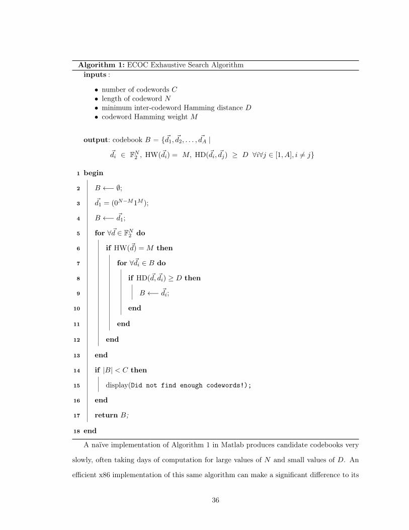
Algorithm 1: ECOC Exhaustive Search Algorithminputs :

• number of codewords C• length of codeword N• minimum inter-codeword Hamming distance D• codeword Hamming weight M

output: codebook B = {d⃗1, d⃗2, . . . , d⃗A |

d⃗i ∈ FN2 , HW(d⃗i) = M, HD(d⃗i, d⃗j) ≥ D ∀i∀j ∈ [1, A], i ̸= j}

1 begin

2 B ←− ∅;

3 d⃗1 = (0N−M1M );

4 B ←− d⃗1;

5 for ∀d⃗ ∈ FN2 do

6 if HW(d⃗) = M then

7 for ∀d⃗i ∈ B do

8 if HD(d⃗, d⃗i) ≥ D then

9 B ←− d⃗i;

10 end

11 end

12 end

13 end

14 if |B| < C then

15 display(Did not find enough codewords!);

16 end

17 return B;

18 end

A naïve implementation of Algorithm 1 in Matlab produces candidate codebooks very

slowly, often taking days of computation for large values of N and small values of D. An

efficient x86 implementation of this same algorithm can make a significant difference to its

36

execution time. The following optimizations can be performed to improve performance of

a naïve implementation by an order of magnitude:

• instead of using the Matlab interpreter, implement the algorithm in a low-level compiled

language such as C or assembly

• instead of representing codewords in a vectorized data structure (where each vector

element can be addressed separately), use a basic unsigned integer type (32, 64 or

128 bits wide)

• instead of using a slow function to implement the Hamming Weight function, HW(d⃗),

make use of a compiler intrinsic such as __builtin_popcountll() in the gcc4 compiler.

Intrinsics enable the programmer to make reference to some basic functionality that

might be handled natively by a particular CPU thereby replacing the need for inline

assembly. If the basic functionality is not supported by the target CPU, the compiler

substitutes equivalent functionality from a software library. For recent Intel x86

processors supporting SSE4.2 extensions, there is an assembly instruction called

POPCNT that returns the number of bits set in an integer operand. In the specific

case of gcc4, in the absence of CPU support for the POPCNT instruction, the supplied

library-equivalent function is not optimal; the variable-precision SWAR algorithm [10]

is roughly twice as fast.

• instead of iterating through all possible 2N possible integers to find theNM

candi-

dates that have a Hamming weight of M , employ a more efficient bit permutation

procedure [2] described in Algorithm 2. This procedure takes an integer candidate

with Hamming weight M as input and returns the next largest integer with the same

Hamming weight as the input. In line 2, a temporary value t is produced that corre-

sponds to the input v with all of its trailing zero bits set to ones. In line 4, CTZ(v)

counts the number of trailing zeros in its argument. This is most efficiently imple-

mented by the x86 bit-scan-forward assembly instruction BSF that should hopefully

be emitted by the appropriate compiler intrinsic such as __builtin_ctzll in the gcc4

compiler. Lines 3, 5 and 6 are responsible for changing the least significant 0’s of v to

37

1’s. In line 7, the arithmetic addition of 1 to t sets the highest new 1-bit in the output

integer w. As an example, if v = 010110002, t = 010110002∨010101112 = 010111112,

s = 101000002, r = 3 + 1 = 4, and w = (((s ∧ −s) − 1) ≫ r) ∨ (t + 1) =

(((s ∧ 011000002)− 1≫ 4) ∨ (011000002) = (((001000002)− 1≫ 4) ∨ (011000002) =

((000111112 ≫ 4) ∨ (011000002) = 000000012 ∨ 011000002 = 011000012. If the

algorithm is run again with the the previously obtained output value, the next great-

est integer with Hamming weight 3 will be produced. The next few integers that

would be produced by the sequence generator are: 011000102, 011001002, 011100002,

and 100000112. To calculate how many times this procedure should be run and to

pre-allocate the maximum amount of storage that will be required, the binomial coef-

ficientNM

can be efficiently calculated by use of the ln Γ(·) function which computes

the natural logarithm of absolute value of the Gamma function. This function is

widely available in many standard libraries (e.g. the C standard math library includes

lgamma). The number of times that Algorithm 2 should be repeated to enumerate all

integers with bit length N and Hamming weight M is:N

M

=0.5 + eln Γ(N+1)−ln Γ(M+1)−ln Γ(N−M+1)

(4.9)

One general caveat regarding this permutation technique is that the codeword lengths

are restricted by the size of the built-in integer types, so the maximum length of

producible codewords is 64 bits. For larger codewords, the GNU Multiple Precision

Arithmetic Library could be used as it has support for integer types of arbitrary size

and the required logical and bit manipulations [12].

38

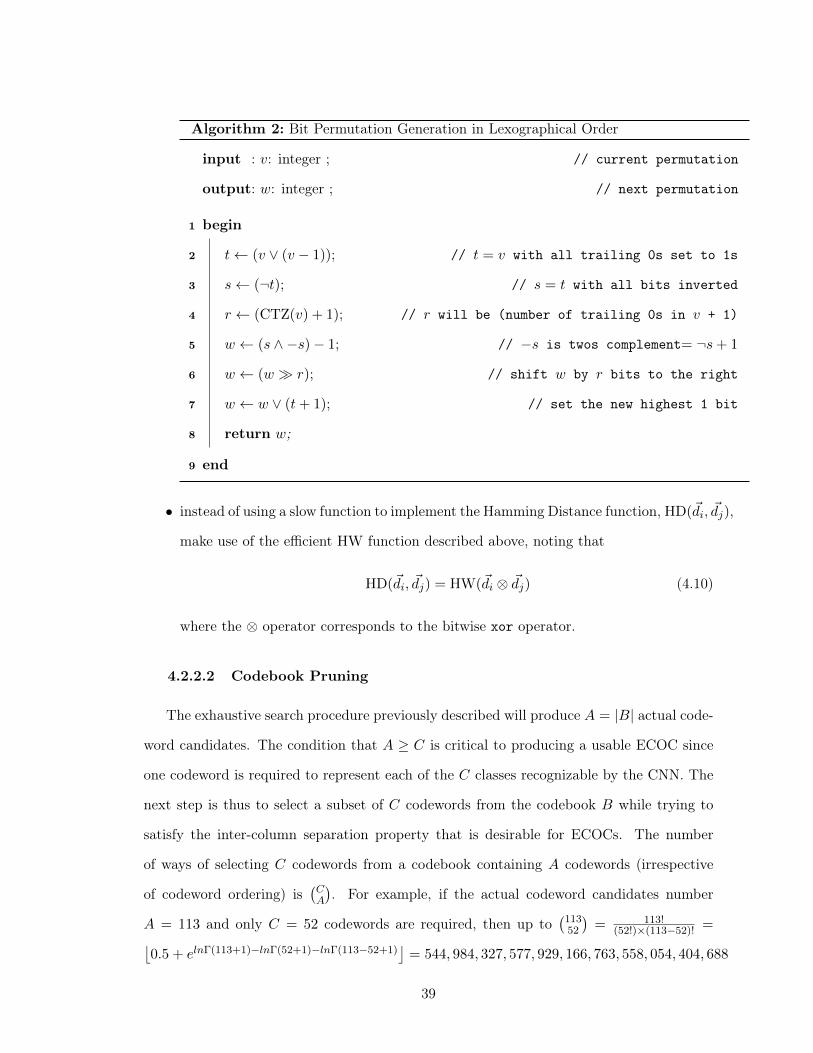
Algorithm 2: Bit Permutation Generation in Lexographical Order

input : v: integer ; // current permutation

output: w: integer ; // next permutation

1 begin

2 t← (v ∨ (v − 1)); // t = v with all trailing 0s set to 1s

3 s← (¬t); // s = t with all bits inverted

4 r ← (CTZ(v) + 1); // r will be (number of trailing 0s in v + 1)

5 w ← (s ∧ −s)− 1; // −s is twos complement= ¬s+ 1

6 w ← (w ≫ r); // shift w by r bits to the right

7 w ← w ∨ (t+ 1); // set the new highest 1 bit

8 return w;

9 end

• instead of using a slow function to implement the Hamming Distance function, HD(d⃗i, d⃗j),

make use of the efficient HW function described above, noting that

HD(d⃗i, d⃗j) = HW(d⃗i ⊗ d⃗j) (4.10)

where the ⊗ operator corresponds to the bitwise xor operator.

4.2.2.2 Codebook Pruning

The exhaustive search procedure previously described will produce A = |B| actual code-

word candidates. The condition that A ≥ C is critical to producing a usable ECOC since

one codeword is required to represent each of the C classes recognizable by the CNN. The

next step is thus to select a subset of C codewords from the codebook B while trying to

satisfy the inter-column separation property that is desirable for ECOCs. The number

of ways of selecting C codewords from a codebook containing A codewords (irrespective

of codeword ordering) isCA

. For example, if the actual codeword candidates number

A = 113 and only C = 52 codewords are required, then up to11352

= 113!

(52!)×(113−52)! =0.5 + elnΓ(113+1)−lnΓ(52+1)−lnΓ(113−52+1)

= 544, 984, 327, 577, 929, 166, 763, 558, 054, 404, 688

39

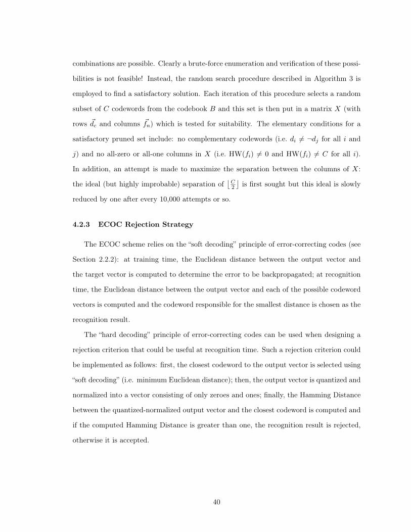
combinations are possible. Clearly a brute-force enumeration and verification of these possi-

bilities is not feasible! Instead, the random search procedure described in Algorithm 3 is

employed to find a satisfactory solution. Each iteration of this procedure selects a random

subset of C codewords from the codebook B and this set is then put in a matrix X (with

rows d⃗c and columns f⃗n) which is tested for suitability. The elementary conditions for a

satisfactory pruned set include: no complementary codewords (i.e. di ̸= ¬dj for all i and

j) and no all-zero or all-one columns in X (i.e. HW(fi) ̸= 0 and HW(fi) ̸= C for all i).

In addition, an attempt is made to maximize the separation between the columns of X:

the ideal (but highly improbable) separation ofC2

is first sought but this ideal is slowly

reduced by one after every 10,000 attempts or so.

4.2.3 ECOC Rejection Strategy

The ECOC scheme relies on the “soft decoding” principle of error-correcting codes (see

Section 2.2.2): at training time, the Euclidean distance between the output vector and

the target vector is computed to determine the error to be backpropagated; at recognition

time, the Euclidean distance between the output vector and each of the possible codeword

vectors is computed and the codeword responsible for the smallest distance is chosen as the

recognition result.

The “hard decoding” principle of error-correcting codes can be used when designing a

rejection criterion that could be useful at recognition time. Such a rejection criterion could

be implemented as follows: first, the closest codeword to the output vector is selected using

“soft decoding” (i.e. minimum Euclidean distance); then, the output vector is quantized and

normalized into a vector consisting of only zeroes and ones; finally, the Hamming Distance

between the quantized-normalized output vector and the closest codeword is computed and

if the computed Hamming Distance is greater than one, the recognition result is rejected,

otherwise it is accepted.

40

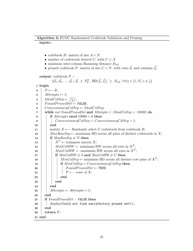
Algorithm 3: ECOC Randomized Codebook Validation and Pruninginputs :

• codebook B: matrix of size A×N• number of codewords desired C, with C ≤ A• minimum inter-column Hamming distance Dcol

• pruned codebook P : matrix of size C ×N , with rows d⃗c and columns f⃗n

output: codebook P ={d⃗1, d⃗2, . . . , d⃗c | d⃗i ∈ FN

2 , HD(f⃗i, f⃗j) ≥ Dcol ∀i∀j ∈ [1, N ], i ̸= j}1 begin2 P ←− ∅;3 Attempts← 1;4 IdealColSep←

C2

;

5 FoundPrunedSet← FALSE;6 ConcessionaryColSep← IdealColSep;7 while not FoundPrunedSet and Attempts < (IdealColSep × 10000) do8 if Attempts mod 10000 = 0 then9 ConcessionaryColSep← ConcessionaryColSep+ 1;

10 end11 matrix X ←− Randomly select C codewords from codebook B;12 MaxRowSep← maximum HD across all pairs of distinct codewords in X;13 if MaxRowSep ̸= N then14 XT ← transpose matrix X;15 MinColHW ← minimum HW across all rows in XT ;16 MaxColHW ← maximum HW across all rows in XT ;17 if MinColHW ̸= 0 and MaxColHW ̸= C then18 MinColSep← minimum HD across all distinct row pairs of XT ;19 if MinColSep < ConcessionaryColSep then20 FoundPrunedSet← TRUE;21 P ←− rows of X;22 end23 end24 end25 Attempts← Attempts+ 1;26 end27 if FoundPrunedSet = FALSE then28 display(Could not find satisfactory pruned set!);29 end30 return P ;31 end

41

CHAPTER 5. EXPERIMENTS

This chapter describes the experimental methodology followed, presents the results

obtained and discusses how they support the position of this thesis.

5.1 Training Sets

5.1.1 MNIST

The MNIST database of handwritten digits [23] is a well-known benchmark in the

machine learning field. It is composed of 60,000 labelled training images and 10,000 labelled

test images. Each image sample contains a single centred handwritten digit that is repre-

sented in a 28×28 pixel grid by 8-bit grayscale values (0 is white, 255 is black). A sample

image with label ‘8’ is depicted in Figure 5.1. Each image sample has a white border with a

depth of 4 pixels. This extra padding is primarily useful when performing kernel operations

on the image since it can reduce the need for specialized processing to deal with the border

edge cases.

The samples in the training set come from one group of 250 writers, while the samples

in the testing set come from another group of 250 writers. The database represents 10

classes labelled ‘0’, ‘1’, ‘2’, ‘3’, ‘4’, ‘5’, ‘6’, ‘7’, ‘8’, ‘9’. While one would expect 6,000

training samples from each class, it is interesting to note that the database creators did

not represent each class equally. Table 5.1 shows the distribution of classes in the MNIST

database.

For this project, five new training sets were created based on the MNIST training set.

These data sets represent a subset of 10,000, 20,000, 30,000, 40,000 and 50,000 images,

respectively, from the original 60,000-image MNIST training set. Care was taken to ensure

42

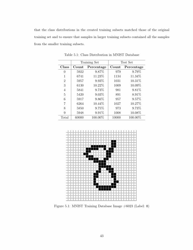
that the class distributions in the created training subsets matched those of the original

training set and to ensure that samples in larger training subsets contained all the samples

from the smaller training subsets.

Table 5.1: Class Distribution in MNIST Database

Training Set Test SetClass Count Percentage Count Percentage

0 5922 9.87% 979 9.79%

1 6741 11.23% 1134 11.34%

2 5957 9.93% 1031 10.31%

3 6130 10.22% 1009 10.09%

4 5841 9.73% 981 9.81%

5 5420 9.03% 891 8.91%

6 5917 9.86% 957 9.57%

7 6264 10.44% 1027 10.27%

8 5850 9.75% 973 9.73%

9 5948 9.91% 1008 10.08%

Total 60000 100.00% 10000 100.00%

Figure 5.1: MNIST Training Database Image #6023 (Label: 8)

43

5.1.2 CENPARMI-MPC

The CENPARMI-MPC database is composed of several million isolated machine-printed

characters that were printed on a 300 dpi monochrome laser printer and were subsequently

scanned (digitized) at a resolution of 300 dpi. The database represents 80 characters (upper-

case and lowercase English letters, numeric digits and special symbols) in several typefaces,

sizes, styles and thicknesses. For this project, training and testing datasets were created

from the CENPARMI-MPC database as two disjoint subsets. For these datasets, approx-

imately 2 samples for the training set and 3 samples for the test set were selected for

each combination of attribute values presented in Table 5.2. This procedure yielded 39,804

labelled training images and 59,706 labelled test images.

Table 5.2: Attribute Name and Values in CENPARMI-MPC Database

Attribute Name Attribute ValuesTypefaces (9) Arial

Bookman Old StyleCentury GothicCourier NewGeorgiaHelvetica CondensedPalatino LinotypeTahomaTimes New Roman

Sizes (3) 81118

Styles (4) NormalBoldItalicBold Italic

Thickness (3) 123

Characters (62) A-Z, a-z, 0-9

Each image sample contains a single centred machine-printed character that is repre-

sented in a 28 × 28 pixel grid by 8-bit grayscale values (0 is white, 255 is black). A sample

44

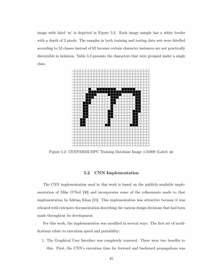
image with label ‘m’ is depicted in Figure 5.2. Each image sample has a white border

with a depth of 2 pixels. The samples in both training and testing data sets were labelled

according to 52 classes instead of 62 because certain character instances are not practically

discernible in isolation. Table 5.3 presents the characters that were grouped under a single

class.

Figure 5.2: CENPARMI-MPC Training Database Image #31000 (Label: m)

5.2 CNN Implementation

The CNN implementation used in this work is based on the publicly-available imple-

mentation of Mike O’Neil [30] and incorporates some of the refinements made to that

implementation by Ishtiaq Khan [21]. This implementation was attractive because it was

released with extensive documentation describing the various design decisions that had been

made throughout its development.

For this work, the implementation was modified in several ways. The first set of modi-

fications relate to execution speed and portability:

1. The Graphical User Interface was completely removed. There were two benefits to

this. First, the CNN’s execution time for forward and backward propagations was

45

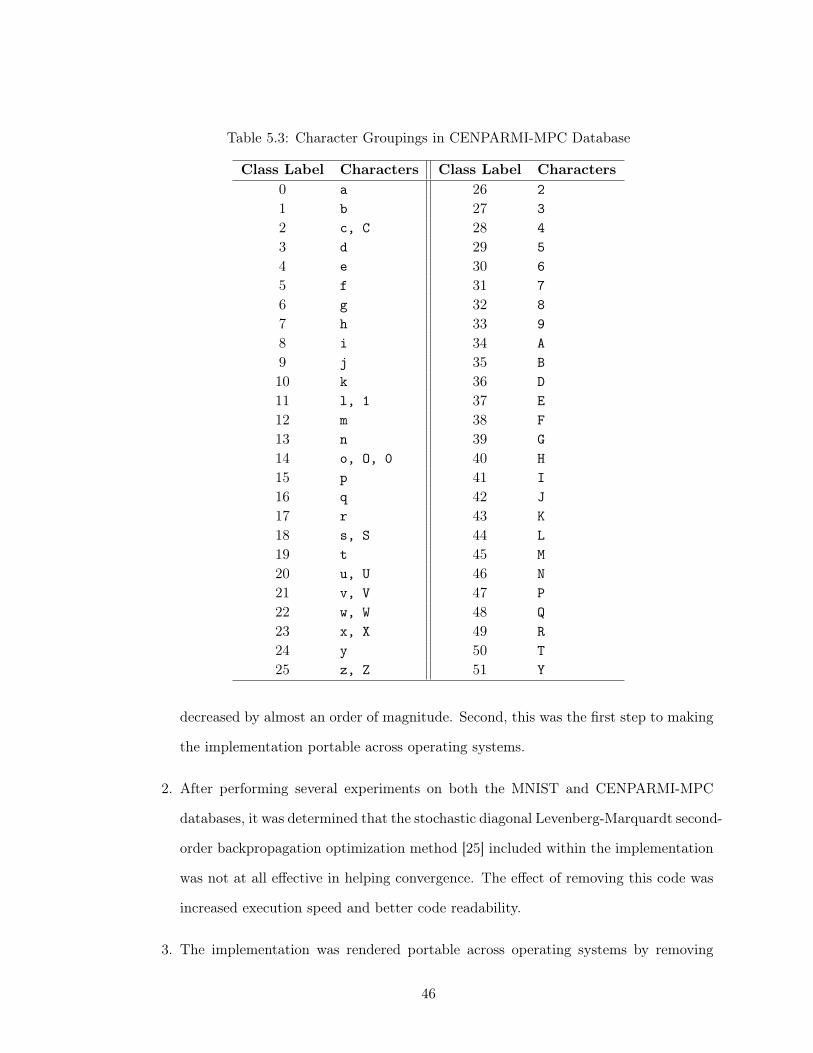
Table 5.3: Character Groupings in CENPARMI-MPC Database

Class Label Characters Class Label Characters0 a 26 21 b 27 32 c, C 28 43 d 29 54 e 30 65 f 31 76 g 32 87 h 33 98 i 34 A9 j 35 B10 k 36 D11 l, 1 37 E12 m 38 F13 n 39 G14 o, O, 0 40 H15 p 41 I16 q 42 J17 r 43 K18 s, S 44 L19 t 45 M20 u, U 46 N21 v, V 47 P22 w, W 48 Q23 x, X 49 R24 y 50 T25 z, Z 51 Y

decreased by almost an order of magnitude. Second, this was the first step to making

the implementation portable across operating systems.

2. After performing several experiments on both the MNIST and CENPARMI-MPC

databases, it was determined that the stochastic diagonal Levenberg-Marquardt second-

order backpropagation optimization method [25] included within the implementation

was not at all effective in helping convergence. The effect of removing this code was

increased execution speed and better code readability.

3. The implementation was rendered portable across operating systems by removing

46

all Windows-specific references and by eliminating all dependencies on third-party

libraries.

4. The code building environment was moved to GNU LLVM g++ 4.2. After conducting

a series of experiments, it was determined that when full compiler optimizations are

used (-O4 option), this compiler generates code that executes 5-10% faster than the

equivalent code generated by either the GNU g++ or the MSVC compilers. This may

be due to the fact that the LLVM compiler performs more sophisticated optimizations

across module boundaries.

The second set of modifications relate to functionality:

1. The architecture of the CNN was made configurable at run-time. Previously the

network’s architecture (number of layers, number of neurons in each layer) was hard-

coded statically within the library. This change made it possible to experiment with

different network topologies without requiring recompilation of the library.

2. Support was added for two types of network output coding (ECOC and Place Coding)

3. Support was added for recognition rejection and confidence metrics

4. The training mode program flow was modified so that at the end of every epoch, a

testing run would be executed over the entire training set (to calculate the training

set error at the end of the epoch) followed by another testing run executed over the

entire test set (to calculate the test set error at the end of the epoch). Through this

modification it was possible to observe training progress more closely and understand

just how much training was minimally required to achieve a well-performing network.

5.3 CNN Configuration

For the experiments carried out, most of the CNN configuration and hyper-parameters

were kept constant. The full configuration is presented below:

1. CNN Architecture:

47

• input layer: 28× 28 = 784 units

• convolutional/subsampling layer: 6 feature maps of size 13×13 (using punctured

5 × 5 convolutional kernels that simultaneously yield convolution and subsam-

pling of factor 2)

• convolutional/subsampling layer: 50 feature maps of size 5× 5 (using punctured

5 × 5 convolutional kernels that simultaneously yield convolution and subsam-

pling of factor 2)

• fully-connected general-purpose classification layer: 100 units

• fully-connected output layer of size C for place-coding networks and size N for

ECOC networks, where C denotes the number of classes to be recognized and

N denotes the length of the codewords in the selected codebook

2. The hyperbolic tangent function was used for all activation functions throughout the

network:

g(x) = 1.7159 · tanh2

3x

(5.1)

3. The activation function was used between layers 2 and 3, 3 and 4, and 4 and 5.

4. The weights were initialized with random values from a uniform distribution U ∼

[−0.05,+0.05] for all layers. Recently published findings involving the effect of weight

initialization for networks using hyperbolic tangent function [3] indicate that superior

results are obtained when the random values are chosen from the uniform distribution

U ∼−

√6√

fanin+fanout,

√6√

fanin+fanout

, where fanin and fanout represent the respec-

tive number of neurons in the previous layer and the next layer that the given neuron

is connected to. These results however were not available at the time the experiments

were initially conducted.

5. The CNNs were trained using the standard backpropagation algorithm with no momen-

tum or second-order methods applied.

48

6. After much experimentation, it was determined that using a fixed learning rate of

η = 0.00005 yielded good general results. This learning rate was reduced by a

factor of 13 every 50 epochs but this reduction made only a slight improvement to the

convergence of the training algorithm in most cases.

7. During training, the complete set of network weights was updated after the backprop-

agation of each training sample.

8. For models trained using distortions, each epoch of the training procedure involves

iterating through the complete set of original training images and, for each image:

(a) generating the two required displacement fields ∆X(x, y) and ∆Y (x, y), which

in turn involves

• following the procedure outlined in Section 4.1.2.1 for generating an affine

scaling distortion with kh = kv picked from a uniform distribution U ∼

[−0.1,+0.1] (i.e. random scaling up to ±10%)

• following the procedure outlined in Section 4.1.2.2 for generating an affine

rotational distortion with α picked from a uniform distribution U ∼ [−5.0, 5.0]

(i.e. random rotation up to ±5◦)

• following the procedure outlined in Section 4.1.2.3 for generating a random

elastic distortion with K = 21, σ = 4.0, and β = 0.34

(b) applying the random displacement field to the original training image

(c) forward propagating the distorted image through the network and computing

the output error

(d) backward propagating this output error through the network and updating the

set of network weights accordingly

It is interesting to note that at no time was the training set ever presented to the

network in its original, non-distorted form.

49

9. The training stop criterion is triggered at the end of the epoch in which at least one

of the following conditions is met:

• 400 training epochs have been completed

• the error rate on the training set (never with distortions) is less than 0.15%

• the error rate on the training set over the last 10 epochs is constant

• the error rate on the training set 20 epochs ago is less than the current training

error rate

• the error rate on the validation test set (if used) is less than 0.1%

10. The error function used was the simple mean-squared error function. This is despite

the fact that there have been many published findings indicating that the cross-

entropy error yields CNNs with lower test errors.

11. The input to the CNN (distorted or not) was normalized from grayscale intensity

values in the range [0, 255] to the range [−1.0,+1.0] which is the appropriate input

range for the chosen hyperbolic tangent activation function.

5.4 Baseline Experiments

The objective of the first set of experiments conducted was to establish the base-

line results for the CNN whose configuration was described in the previous section. A

total of 14 baseline models were trained using CNNs with output place coding: 6 MNIST

models (MNIST-10K, MNIST-20K, MNIST-30K, MNIST-40K, MNIST-50K, MNIST-60K)

trained without distortions, 6 MNIST models (MNIST-10K, MNIST-20K, MNIST-30K,

MNIST-40K, MNIST-50K, MNIST-60K) trained with distortions, 1 CENPARMI-MPC

model trained without distortions, and 1 CENPARMI-MPC model trained with distor-

tions. The learning curves which show the progressive improvement in test and training

error rates at the conclusion of each training epoch are depicted in Figures 5.3, 5.4, 5.5,

and 5.6, respectively. The final training and testing error rates for the baseline models are

summarized in Table 5.4.

50

Table 5.4: Summary of Baseline Error Rates

Data SetWithout Distortions With Distortions

Training Error Testing Error Training Error Testing ErrorMNIST-10K 0.15% 2.53% 0.70% 1.58%MNIST-20K 0.16% 1.74% 0.64% 1.07%MNIST-30K 0.14% 1.43% 0.56% 0.82%MNIST-40K 0.13% 1.34% 0.62% 0.89%MNIST-50K 0.17% 1.24% 0.59% 0.79%MNIST-60K 0.15% 1.28% 0.55% 0.76%

CENPARMI-MPC 0.41% 0.54% 0.63% 0.63%

51

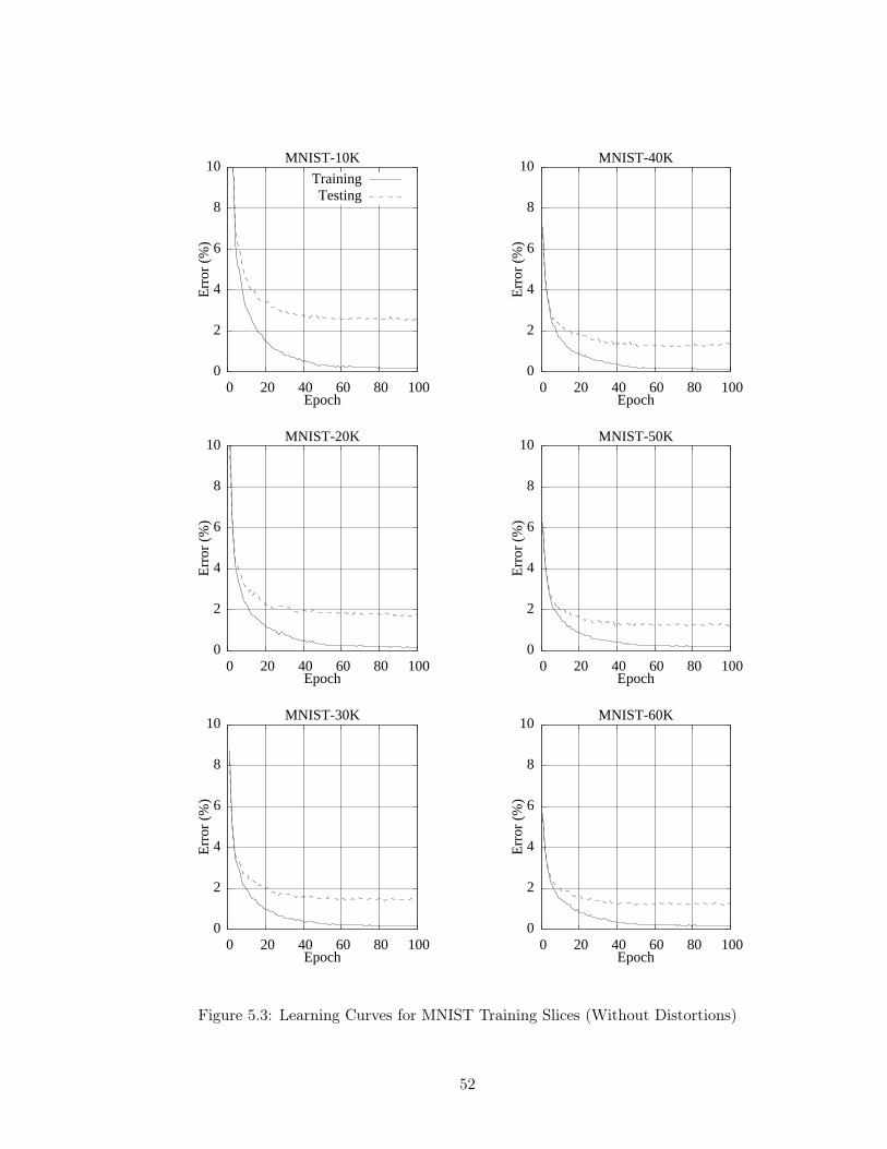
0

2

4

6

8

10

0 20 40 60 80 100

Erro

r (%

)

Epoch

MNIST-10KTrainingTesting

0

2

4

6

8

10

0 20 40 60 80 100

Erro

r (%

)

Epoch

MNIST-20K

0

2

4

6

8

10

0 20 40 60 80 100

Erro

r (%

)

Epoch

MNIST-30K

0

2

4

6

8

10

0 20 40 60 80 100

Erro

r (%

)

Epoch

MNIST-40K

0

2

4

6

8

10

0 20 40 60 80 100

Erro

r (%

)

Epoch

MNIST-50K

0

2

4

6

8

10

0 20 40 60 80 100

Erro

r (%

)

Epoch

MNIST-60K

Figure 5.3: Learning Curves for MNIST Training Slices (Without Distortions)

52

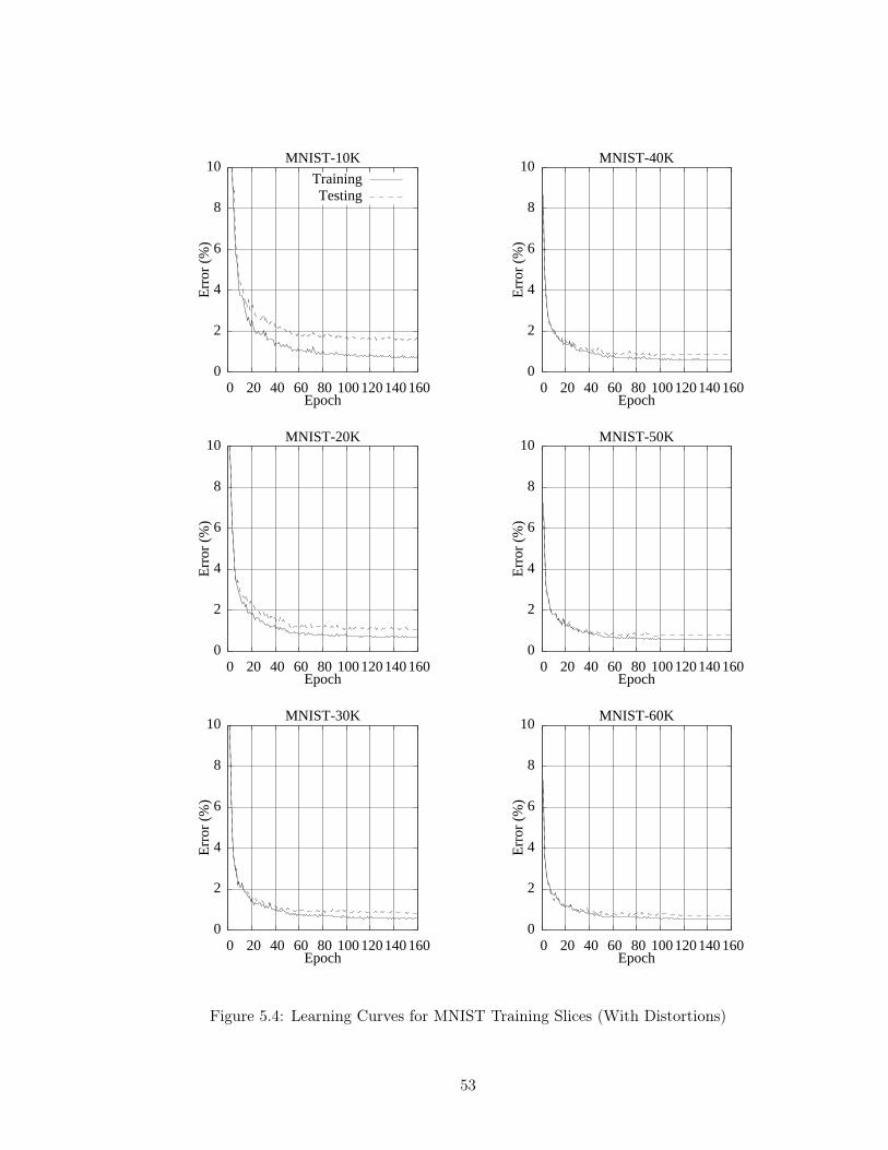
0

2

4

6

8

10

0 20 40 60 80 100 120 140 160

Erro

r (%

)

Epoch

MNIST-10KTrainingTesting

0

2

4

6

8

10

0 20 40 60 80 100 120 140 160

Erro

r (%

)

Epoch

MNIST-20K

0

2

4

6

8

10

0 20 40 60 80 100 120 140 160

Erro

r (%

)

Epoch

MNIST-30K

0

2

4

6

8

10

0 20 40 60 80 100 120 140 160

Erro

r (%

)

Epoch

MNIST-40K

0

2

4

6

8

10

0 20 40 60 80 100 120 140 160

Erro

r (%

)

Epoch

MNIST-50K

0

2

4

6

8

10

0 20 40 60 80 100 120 140 160

Erro

r (%

)

Epoch

MNIST-60K

Figure 5.4: Learning Curves for MNIST Training Slices (With Distortions)

53

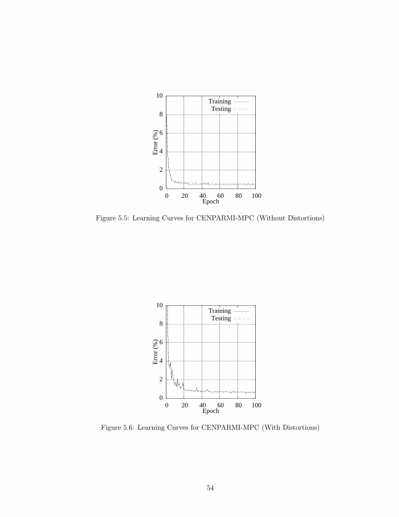
0

2

4

6

8

10

0 20 40 60 80 100

Erro

r (%

)

Epoch

TrainingTesting

Figure 5.5: Learning Curves for CENPARMI-MPC (Without Distortions)

0

2

4

6

8

10

0 20 40 60 80 100

Erro

r (%

)

Epoch

TrainingTesting

Figure 5.6: Learning Curves for CENPARMI-MPC (With Distortions)

54

The results for the MNIST data sets clearly indicate that larger training sets produce

smaller testing errors: the relative testing error for the MNIST-10K data set is reduced

by approximately 50% when compared to the performance achieved by the MNIST-60K

data set. Also for the MNIST data sets, the relative testing error is reduced by approx-

imately 40% for the same sized training set when training distortions are used. These

results are consistent with what has been reported in the literature [25]. The results for

the CENPARMI-MPC data set indicate that the use of distortions during training actu-

ally increases the relative testing error by approximately 17%. The reason for this can be

explained by the fact that the utilized distortions were designed with the plausible defor-

mation of handwritten digits in mind. The use of elastic distortions was probably not

appropriate for machine-printed characters as these would have only been beneficial in the

event that a substantial number of test set samples were digitized from waterlogged paper!

In order to provide baseline results for the cases where classifier rejection is permitted,

two classic rejection measures are evaluated. After an image has been recognized by the

CNN, the highest output activation value is denoted by α and the second highest output

activation value is denoted by β. The difference between these two values is denoted by

δ. The classic rejection measures involve accepting recognition results that yield a value

of α or δ above a predefined threshold that is arbitrarily set to some value within the

output range [−1.7159,+1.7159]. The ROC curves for the two classic rejection measures

are presented in Figures 5.7, 5.8, 5.9, 5.10 for MNIST (without distortions), MNIST (with

distortions), CENPARMI-MPC (without distortions) and CENPARMI-MPC (with distor-

tions), respectively. Interestingly, the δ threshold metric is superior to the α threshold

metric in every case. This is because the ROC curve for the δ threshold metric lies above

the ROC curve for the α threshold metric. Also, the curves clearly show the superior

performance of models trained with distortions when compared to those training without

distortions. This is because the ROC curves for the models trained with distortions pass

closer to the upper-left corner of the graph than for the models trained without distortions.

55

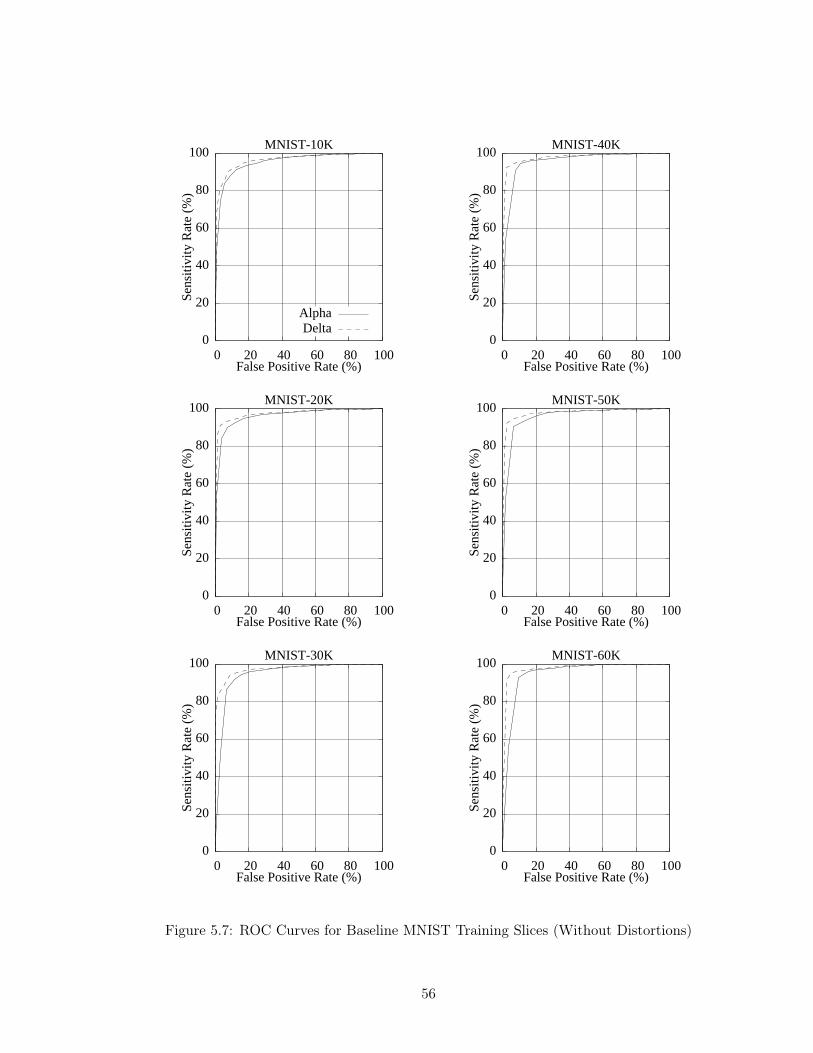
0

20

40

60

80

100

0 20 40 60 80 100

Sens

itivi

ty R

ate

(%)

False Positive Rate (%)

MNIST-10K

AlphaDelta

0

20

40

60

80

100

0 20 40 60 80 100

Sens

itivi

ty R

ate

(%)

False Positive Rate (%)

MNIST-20K

0

20

40

60

80

100

0 20 40 60 80 100

Sens

itivi

ty R

ate

(%)

False Positive Rate (%)

MNIST-30K

0

20

40

60

80

100

0 20 40 60 80 100

Sens

itivi

ty R

ate

(%)

False Positive Rate (%)

MNIST-40K

0

20

40

60

80

100

0 20 40 60 80 100

Sens

itivi

ty R

ate

(%)

False Positive Rate (%)

MNIST-50K

0

20

40

60

80

100

0 20 40 60 80 100

Sens

itivi

ty R

ate

(%)

False Positive Rate (%)

MNIST-60K

Figure 5.7: ROC Curves for Baseline MNIST Training Slices (Without Distortions)

56

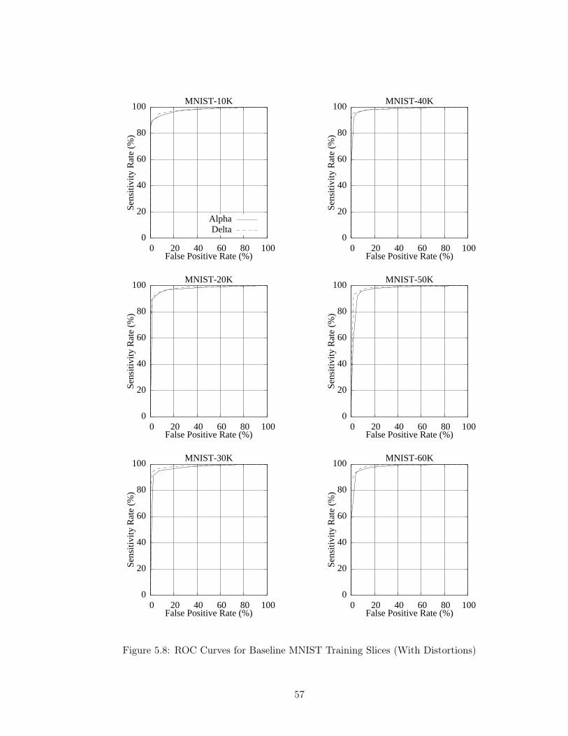
0

20

40

60

80

100

0 20 40 60 80 100

Sens

itivi

ty R

ate

(%)

False Positive Rate (%)

MNIST-10K

AlphaDelta

0

20

40

60

80

100

0 20 40 60 80 100

Sens

itivi

ty R

ate

(%)

False Positive Rate (%)

MNIST-20K

0

20

40

60

80

100

0 20 40 60 80 100

Sens

itivi

ty R

ate

(%)

False Positive Rate (%)

MNIST-30K

0

20

40

60

80

100

0 20 40 60 80 100

Sens

itivi

ty R

ate

(%)

False Positive Rate (%)

MNIST-40K

0

20

40

60

80

100

0 20 40 60 80 100

Sens

itivi

ty R

ate

(%)

False Positive Rate (%)

MNIST-50K

0

20

40

60

80

100

0 20 40 60 80 100

Sens

itivi

ty R

ate

(%)

False Positive Rate (%)

MNIST-60K

Figure 5.8: ROC Curves for Baseline MNIST Training Slices (With Distortions)

57

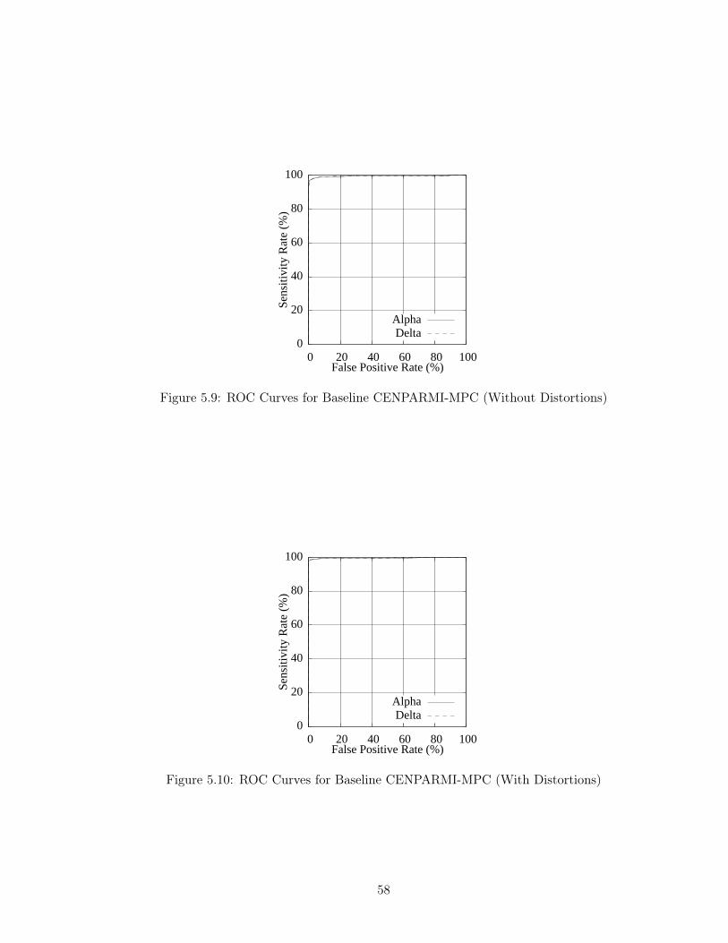
0

20

40

60

80

100

0 20 40 60 80 100

Sens

itivi

ty R

ate

(%)

False Positive Rate (%)

AlphaDelta

Figure 5.9: ROC Curves for Baseline CENPARMI-MPC (Without Distortions)

0

20

40

60

80

100

0 20 40 60 80 100

Sens

itivi

ty R

ate

(%)

False Positive Rate (%)

AlphaDelta

Figure 5.10: ROC Curves for Baseline CENPARMI-MPC (With Distortions)

58

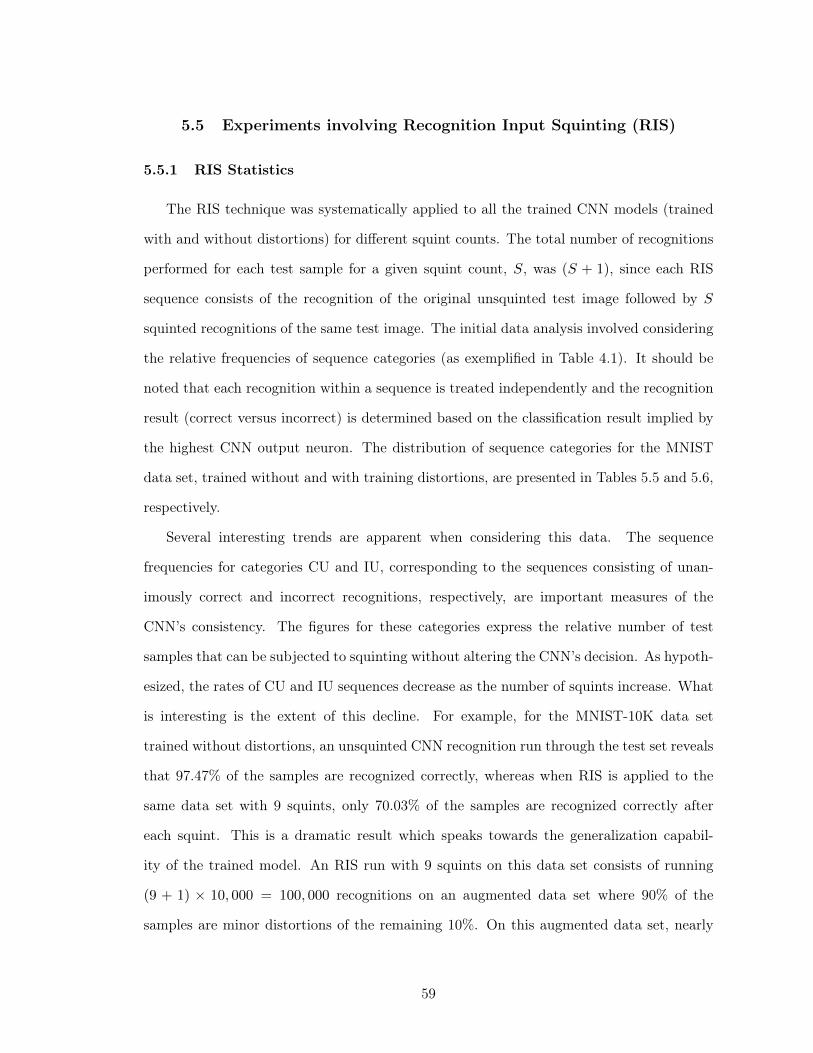
5.5 Experiments involving Recognition Input Squinting (RIS)

5.5.1 RIS Statistics

The RIS technique was systematically applied to all the trained CNN models (trained

with and without distortions) for different squint counts. The total number of recognitions

performed for each test sample for a given squint count, S, was (S + 1), since each RIS

sequence consists of the recognition of the original unsquinted test image followed by S

squinted recognitions of the same test image. The initial data analysis involved considering

the relative frequencies of sequence categories (as exemplified in Table 4.1). It should be

noted that each recognition within a sequence is treated independently and the recognition

result (correct versus incorrect) is determined based on the classification result implied by

the highest CNN output neuron. The distribution of sequence categories for the MNIST

data set, trained without and with training distortions, are presented in Tables 5.5 and 5.6,

respectively.

Several interesting trends are apparent when considering this data. The sequence

frequencies for categories CU and IU, corresponding to the sequences consisting of unan-

imously correct and incorrect recognitions, respectively, are important measures of the

CNN’s consistency. The figures for these categories express the relative number of test

samples that can be subjected to squinting without altering the CNN’s decision. As hypoth-

esized, the rates of CU and IU sequences decrease as the number of squints increase. What

is interesting is the extent of this decline. For example, for the MNIST-10K data set

trained without distortions, an unsquinted CNN recognition run through the test set reveals

that 97.47% of the samples are recognized correctly, whereas when RIS is applied to the

same data set with 9 squints, only 70.03% of the samples are recognized correctly after

each squint. This is a dramatic result which speaks towards the generalization capabil-

ity of the trained model. An RIS run with 9 squints on this data set consists of running

(9 + 1) × 10, 000 = 100, 000 recognitions on an augmented data set where 90% of the

samples are minor distortions of the remaining 10%. On this augmented data set, nearly

59

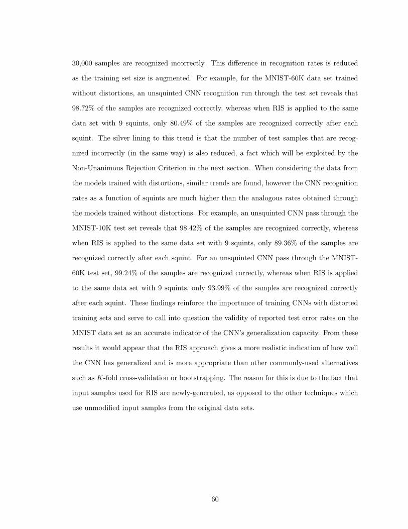
30,000 samples are recognized incorrectly. This difference in recognition rates is reduced

as the training set size is augmented. For example, for the MNIST-60K data set trained

without distortions, an unsquinted CNN recognition run through the test set reveals that

98.72% of the samples are recognized correctly, whereas when RIS is applied to the same

data set with 9 squints, only 80.49% of the samples are recognized correctly after each

squint. The silver lining to this trend is that the number of test samples that are recog-

nized incorrectly (in the same way) is also reduced, a fact which will be exploited by the

Non-Unanimous Rejection Criterion in the next section. When considering the data from

the models trained with distortions, similar trends are found, however the CNN recognition

rates as a function of squints are much higher than the analogous rates obtained through

the models trained without distortions. For example, an unsquinted CNN pass through the

MNIST-10K test set reveals that 98.42% of the samples are recognized correctly, whereas

when RIS is applied to the same data set with 9 squints, only 89.36% of the samples are

recognized correctly after each squint. For an unsquinted CNN pass through the MNIST-

60K test set, 99.24% of the samples are recognized correctly, whereas when RIS is applied

to the same data set with 9 squints, only 93.99% of the samples are recognized correctly

after each squint. These findings reinforce the importance of training CNNs with distorted

training sets and serve to call into question the validity of reported test error rates on the

MNIST data set as an accurate indicator of the CNN’s generalization capacity. From these

results it would appear that the RIS approach gives a more realistic indication of how well

the CNN has generalized and is more appropriate than other commonly-used alternatives

such as K-fold cross-validation or bootstrapping. The reason for this is due to the fact that

input samples used for RIS are newly-generated, as opposed to the other techniques which

use unmodified input samples from the original data sets.

60

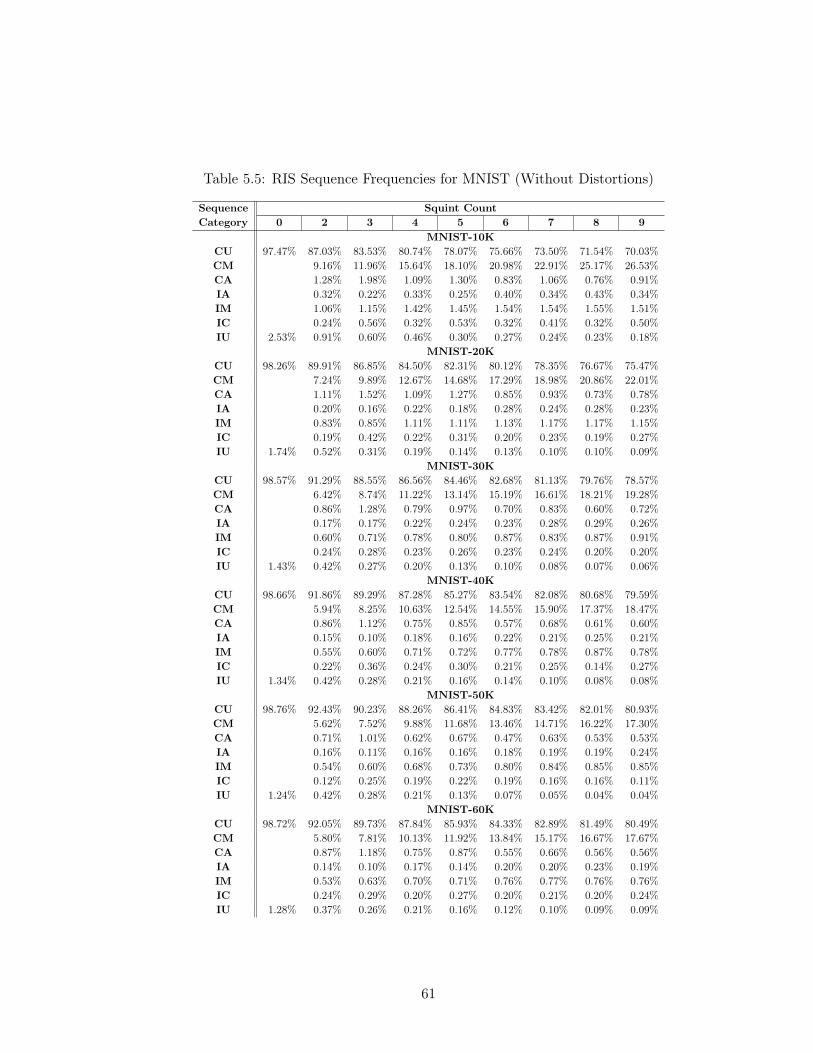
Table 5.5: RIS Sequence Frequencies for MNIST (Without Distortions)

Sequence Squint CountCategory 0 2 3 4 5 6 7 8 9

MNIST-10KCU 97.47% 87.03% 83.53% 80.74% 78.07% 75.66% 73.50% 71.54% 70.03%CM 9.16% 11.96% 15.64% 18.10% 20.98% 22.91% 25.17% 26.53%CA 1.28% 1.98% 1.09% 1.30% 0.83% 1.06% 0.76% 0.91%IA 0.32% 0.22% 0.33% 0.25% 0.40% 0.34% 0.43% 0.34%IM 1.06% 1.15% 1.42% 1.45% 1.54% 1.54% 1.55% 1.51%IC 0.24% 0.56% 0.32% 0.53% 0.32% 0.41% 0.32% 0.50%IU 2.53% 0.91% 0.60% 0.46% 0.30% 0.27% 0.24% 0.23% 0.18%

MNIST-20KCU 98.26% 89.91% 86.85% 84.50% 82.31% 80.12% 78.35% 76.67% 75.47%CM 7.24% 9.89% 12.67% 14.68% 17.29% 18.98% 20.86% 22.01%CA 1.11% 1.52% 1.09% 1.27% 0.85% 0.93% 0.73% 0.78%IA 0.20% 0.16% 0.22% 0.18% 0.28% 0.24% 0.28% 0.23%IM 0.83% 0.85% 1.11% 1.11% 1.13% 1.17% 1.17% 1.15%IC 0.19% 0.42% 0.22% 0.31% 0.20% 0.23% 0.19% 0.27%IU 1.74% 0.52% 0.31% 0.19% 0.14% 0.13% 0.10% 0.10% 0.09%

MNIST-30KCU 98.57% 91.29% 88.55% 86.56% 84.46% 82.68% 81.13% 79.76% 78.57%CM 6.42% 8.74% 11.22% 13.14% 15.19% 16.61% 18.21% 19.28%CA 0.86% 1.28% 0.79% 0.97% 0.70% 0.83% 0.60% 0.72%IA 0.17% 0.17% 0.22% 0.24% 0.23% 0.28% 0.29% 0.26%IM 0.60% 0.71% 0.78% 0.80% 0.87% 0.83% 0.87% 0.91%IC 0.24% 0.28% 0.23% 0.26% 0.23% 0.24% 0.20% 0.20%IU 1.43% 0.42% 0.27% 0.20% 0.13% 0.10% 0.08% 0.07% 0.06%

MNIST-40KCU 98.66% 91.86% 89.29% 87.28% 85.27% 83.54% 82.08% 80.68% 79.59%CM 5.94% 8.25% 10.63% 12.54% 14.55% 15.90% 17.37% 18.47%CA 0.86% 1.12% 0.75% 0.85% 0.57% 0.68% 0.61% 0.60%IA 0.15% 0.10% 0.18% 0.16% 0.22% 0.21% 0.25% 0.21%IM 0.55% 0.60% 0.71% 0.72% 0.77% 0.78% 0.87% 0.78%IC 0.22% 0.36% 0.24% 0.30% 0.21% 0.25% 0.14% 0.27%IU 1.34% 0.42% 0.28% 0.21% 0.16% 0.14% 0.10% 0.08% 0.08%

MNIST-50KCU 98.76% 92.43% 90.23% 88.26% 86.41% 84.83% 83.42% 82.01% 80.93%CM 5.62% 7.52% 9.88% 11.68% 13.46% 14.71% 16.22% 17.30%CA 0.71% 1.01% 0.62% 0.67% 0.47% 0.63% 0.53% 0.53%IA 0.16% 0.11% 0.16% 0.16% 0.18% 0.19% 0.19% 0.24%IM 0.54% 0.60% 0.68% 0.73% 0.80% 0.84% 0.85% 0.85%IC 0.12% 0.25% 0.19% 0.22% 0.19% 0.16% 0.16% 0.11%IU 1.24% 0.42% 0.28% 0.21% 0.13% 0.07% 0.05% 0.04% 0.04%

MNIST-60KCU 98.72% 92.05% 89.73% 87.84% 85.93% 84.33% 82.89% 81.49% 80.49%CM 5.80% 7.81% 10.13% 11.92% 13.84% 15.17% 16.67% 17.67%CA 0.87% 1.18% 0.75% 0.87% 0.55% 0.66% 0.56% 0.56%IA 0.14% 0.10% 0.17% 0.14% 0.20% 0.20% 0.23% 0.19%IM 0.53% 0.63% 0.70% 0.71% 0.76% 0.77% 0.76% 0.76%IC 0.24% 0.29% 0.20% 0.27% 0.20% 0.21% 0.20% 0.24%IU 1.28% 0.37% 0.26% 0.21% 0.16% 0.12% 0.10% 0.09% 0.09%

61

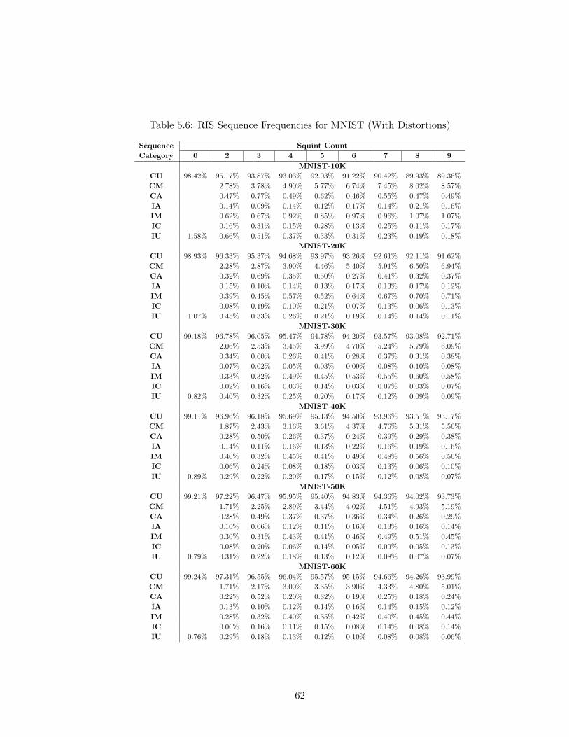
Table 5.6: RIS Sequence Frequencies for MNIST (With Distortions)

Sequence Squint CountCategory 0 2 3 4 5 6 7 8 9

MNIST-10KCU 98.42% 95.17% 93.87% 93.03% 92.03% 91.22% 90.42% 89.93% 89.36%CM 2.78% 3.78% 4.90% 5.77% 6.74% 7.45% 8.02% 8.57%CA 0.47% 0.77% 0.49% 0.62% 0.46% 0.55% 0.47% 0.49%IA 0.14% 0.09% 0.14% 0.12% 0.17% 0.14% 0.21% 0.16%IM 0.62% 0.67% 0.92% 0.85% 0.97% 0.96% 1.07% 1.07%IC 0.16% 0.31% 0.15% 0.28% 0.13% 0.25% 0.11% 0.17%IU 1.58% 0.66% 0.51% 0.37% 0.33% 0.31% 0.23% 0.19% 0.18%

MNIST-20KCU 98.93% 96.33% 95.37% 94.68% 93.97% 93.26% 92.61% 92.11% 91.62%CM 2.28% 2.87% 3.90% 4.46% 5.40% 5.91% 6.50% 6.94%CA 0.32% 0.69% 0.35% 0.50% 0.27% 0.41% 0.32% 0.37%IA 0.15% 0.10% 0.14% 0.13% 0.17% 0.13% 0.17% 0.12%IM 0.39% 0.45% 0.57% 0.52% 0.64% 0.67% 0.70% 0.71%IC 0.08% 0.19% 0.10% 0.21% 0.07% 0.13% 0.06% 0.13%IU 1.07% 0.45% 0.33% 0.26% 0.21% 0.19% 0.14% 0.14% 0.11%

MNIST-30KCU 99.18% 96.78% 96.05% 95.47% 94.78% 94.20% 93.57% 93.08% 92.71%CM 2.06% 2.53% 3.45% 3.99% 4.70% 5.24% 5.79% 6.09%CA 0.34% 0.60% 0.26% 0.41% 0.28% 0.37% 0.31% 0.38%IA 0.07% 0.02% 0.05% 0.03% 0.09% 0.08% 0.10% 0.08%IM 0.33% 0.32% 0.49% 0.45% 0.53% 0.55% 0.60% 0.58%IC 0.02% 0.16% 0.03% 0.14% 0.03% 0.07% 0.03% 0.07%IU 0.82% 0.40% 0.32% 0.25% 0.20% 0.17% 0.12% 0.09% 0.09%

MNIST-40KCU 99.11% 96.96% 96.18% 95.69% 95.13% 94.50% 93.96% 93.51% 93.17%CM 1.87% 2.43% 3.16% 3.61% 4.37% 4.76% 5.31% 5.56%CA 0.28% 0.50% 0.26% 0.37% 0.24% 0.39% 0.29% 0.38%IA 0.14% 0.11% 0.16% 0.13% 0.22% 0.16% 0.19% 0.16%IM 0.40% 0.32% 0.45% 0.41% 0.49% 0.48% 0.56% 0.56%IC 0.06% 0.24% 0.08% 0.18% 0.03% 0.13% 0.06% 0.10%IU 0.89% 0.29% 0.22% 0.20% 0.17% 0.15% 0.12% 0.08% 0.07%

MNIST-50KCU 99.21% 97.22% 96.47% 95.95% 95.40% 94.83% 94.36% 94.02% 93.73%CM 1.71% 2.25% 2.89% 3.44% 4.02% 4.51% 4.93% 5.19%CA 0.28% 0.49% 0.37% 0.37% 0.36% 0.34% 0.26% 0.29%IA 0.10% 0.06% 0.12% 0.11% 0.16% 0.13% 0.16% 0.14%IM 0.30% 0.31% 0.43% 0.41% 0.46% 0.49% 0.51% 0.45%IC 0.08% 0.20% 0.06% 0.14% 0.05% 0.09% 0.05% 0.13%IU 0.79% 0.31% 0.22% 0.18% 0.13% 0.12% 0.08% 0.07% 0.07%

MNIST-60KCU 99.24% 97.31% 96.55% 96.04% 95.57% 95.15% 94.66% 94.26% 93.99%CM 1.71% 2.17% 3.00% 3.35% 3.90% 4.33% 4.80% 5.01%CA 0.22% 0.52% 0.20% 0.32% 0.19% 0.25% 0.18% 0.24%IA 0.13% 0.10% 0.12% 0.14% 0.16% 0.14% 0.15% 0.12%IM 0.28% 0.32% 0.40% 0.35% 0.42% 0.40% 0.45% 0.44%IC 0.06% 0.16% 0.11% 0.15% 0.08% 0.14% 0.08% 0.14%IU 0.76% 0.29% 0.18% 0.13% 0.12% 0.10% 0.08% 0.08% 0.06%

62

5.5.2 RIS Rejection Criteria and Confidence Metric

5.5.2.1 Rejection of Non-Unanimous RIS Sequences

This rejection criterion involves rejecting any training sample that does not produce a

unanimous RIS sequence. For a given RIS sequence, the rejection and precision rates are

computed as follows:

rejection rate = 100% – CU – IU = CM + CA + IA + IM + IC

precision rate = CUCU+IU × 100%

Table 5.7 depicts the results of these computations on the MNIST data sets trained

without and with distortions. There is an improvement of precision as the number of squints

in a given RIS sequence is increased, but also an increase to the number of samples that

must be rejected to achieve this precision. Overall this rejection criterion works very well,

particularly on the models trained on the smallest data sets. For example, the MNIST-

10K model trained without distortions is able to achieve a 99.74% precision rate after

rejecting 29.79% of the samples when 9 squints are performed. This corresponds to a

relative improvement of 2.33% on the precision rate when compared to the baseline non-

RIS case. For the MNIST-50K model trained without distortions, a 99.95% precision rate

was achieved after rejecting 16.53% of the samples when 7 squints are performed. This

corresponds to a relative improvement of 1.20% on the precision rate when compared to

the baseline non-RIS case. When considering the models trained with distortions, similar

trends are observed, although the relative gains in precision are more modest since the

baseline results were already quite good to begin with. What is important to note with

these models is the high performance that is achieved with a relatively low rejection rate.

For example, the MNIST-10K model trained with distortions is able to achieve a 99.80%

precision rate after rejecting 10.46% of the samples when 9 squints are performed. For

the MNIST-60K model trained with distortions, a 99.94% precision rate was achieved after

rejecting only 5.95% of the samples.

63

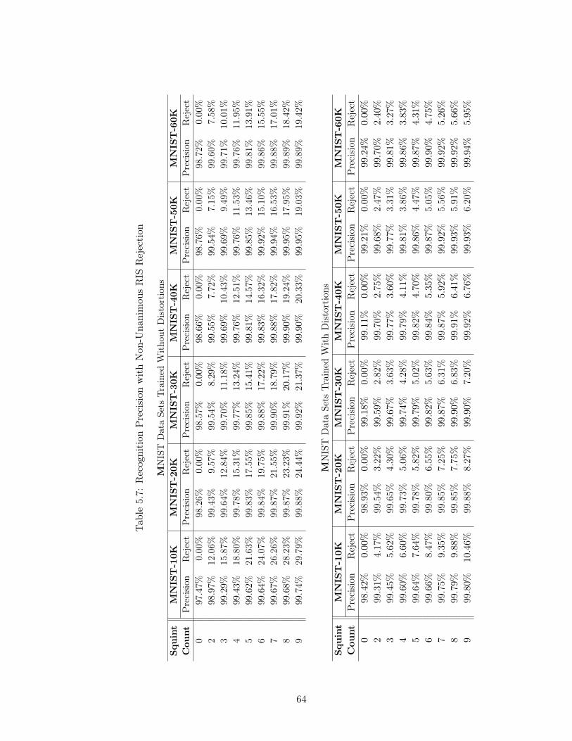
Tab

le5.

7:R

ecog

niti

onP

reci

sion

wit

hN

on-U

nani

mou

sR

ISR

ejec

tion

MN

IST

Dat

aSe

tsTra

ined

Wit

hout

Dis

tort

ions

Squ

int

MN

IST

-10K

MN

IST

-20K

MN

IST

-30K

MN

IST

-40K

MN

IST

-50K

MN

IST

-60K

Cou

ntP

reci

sion

Rej

ect

Pre

cisi

onR

ejec

tP

reci

sion

Rej

ect

Pre

cisi

onR

ejec

tP

reci

sion

Rej

ect

Pre

cisi

onR

ejec

t0

97.4

7%0.

00%

98.2

6%0.

00%

98.5

7%0.

00%

98.6

6%0.

00%

98.7

6%0.

00%

98.7

2%0.

00%

298

.97%

12.0

6%99

.43%

9.57

%99

.54%

8.29

%99

.55%

7.72

%99

.54%

7.15

%99

.60%

7.58

%3

99.2

9%15

.87%

99.6

4%12

.84%

99.7

0%11

.18%

99.6

9%10

.43%

99.6

9%9.

49%

99.7

1%10

.01%

499

.43%

18.8

0%99

.78%

15.3

1%99

.77%

13.2

4%99

.76%

12.5

1%99

.76%

11.5

3%99

.76%

11.9

5%5

99.6

2%21

.63%

99.8

3%17

.55%

99.8

5%15

.41%

99.8

1%14

.57%

99.8

5%13

.46%

99.8

1%13

.91%

699

.64%

24.0

7%99

.84%

19.7

5%99

.88%

17.2

2%99

.83%

16.3

2%99

.92%

15.1

0%99

.86%

15.5

5%7

99.6

7%26

.26%

99.8

7%21

.55%

99.9

0%18

.79%

99.8

8%17

.82%

99.9

4%16

.53%

99.8

8%17

.01%

899

.68%

28.2

3%99

.87%

23.2

3%99

.91%

20.1

7%99

.90%

19.2

4%99

.95%

17.9

5%99

.89%

18.4

2%9

99.7

4%29

.79%

99.8

8%24

.44%

99.9

2%21

.37%

99.9

0%20

.33%

99.9

5%19

.03%

99.8

9%19

.42%

MN

IST

Dat

aSe

tsTra

ined

Wit

hD

isto

rtio

nsSqu

int

MN

IST

-10K

MN

IST

-20K

MN

IST

-30K

MN

IST

-40K

MN

IST

-50K

MN

IST

-60K

Cou

ntP

reci

sion

Rej

ect

Pre

cisi

onR

ejec

tP

reci

sion

Rej

ect

Pre

cisi

onR

ejec

tP

reci

sion

Rej

ect

Pre

cisi

onR

ejec

t0

98.4

2%0.

00%

98.9

3%0.

00%

99.1

8%0.

00%

99.1

1%0.

00%

99.2

1%0.

00%

99.2

4%0.

00%

299

.31%

4.17

%99

.54%

3.22

%99

.59%

2.82

%99

.70%

2.75

%99

.68%

2.47

%99

.70%

2.40

%3

99.4

5%5.

62%

99.6

5%4.

30%

99.6

7%3.

63%

99.7

7%3.

60%

99.7

7%3.

31%

99.8

1%3.

27%

499

.60%

6.60

%99

.73%

5.06

%99

.74%

4.28

%99

.79%

4.11

%99

.81%

3.86

%99

.86%

3.83

%5

99.6

4%7.

64%

99.7

8%5.

82%

99.7

9%5.

02%

99.8

2%4.

70%

99.8

6%4.

47%

99.8

7%4.

31%

699

.66%

8.47

%99

.80%

6.55

%99

.82%

5.63

%99

.84%

5.35

%99

.87%

5.05

%99

.90%

4.75

%7

99.7

5%9.

35%

99.8

5%7.

25%

99.8

7%6.

31%

99.8

7%5.

92%

99.9

2%5.

56%

99.9

2%5.

26%

899

.79%

9.88

%99

.85%

7.75

%99

.90%

6.83

%99

.91%

6.41

%99

.93%

5.91

%99

.92%

5.66

%9

99.8

0%10

.46%

99.8

8%8.

27%

99.9

0%7.

20%

99.9

2%6.

76%

99.9

3%6.

20%

99.9

4%5.

95%

64

5.5.2.2 Rejection of Non-Majority RIS Sequences

This rejection criterion involves rejecting any training sample that does not produce

a clear majority RIS sequence. For a given RIS sequence, the relative frequencies of RIS

sequence elements (i.e. unique recognition results) are computed and any sequences that

contain the same frequency count for the top two or more elements are rejected.

Table 5.8 depicts the results of these computations on the MNIST data sets trained

without and with distortions. Since most RIS sequences contain a clear majority, there

are relatively few rejections, however in the vast majority of cases, the rejections do help

in driving the precision rate up, particularly in the cases trained with smaller data sets.

For example, for the model trained on the MNIST-10K data set without distortions, the

precision rate was increased from 97.47% to 97.63% by using 9 squints and rejecting only

75 samples from the 10,000 image test set.

5.5.2.3 Rejection of Sequences With Confidence Score Below A Fixed Thresh-

old

The Non-Unanimity rejection criterion provides different precision and rejection rates

by varying the number of squints. In cases where the number of squints is a fixed parameter,

it is useful to have another parameter that can be used to reduce the rejection rate even if

at the expense of the recognition precision. The Confidence Score presented in Section 4.1.3

is used here for this purpose. The rejection curves for this rejection criterion are presented

in Figures 5.11 and 5.12 for models trained on the MNIST database slices, without and

with distortions, respectively. There are several interesting observations that can be made

from studying these curves. First, the rightmost point of each curve (highest rejection rate)

corresponds to the highest precision attainable for a particular MNIST training slice and

a fixed squint count. This ideal precision can never exceed the result obtained through

the Rejection of Non-Unanimous RIS Sequences criterion, since the Confidence Score is

designed to yield 100% certainty in the case of unanimous RIS sequences and to penalize

sequences proportionately to how much they diverge from this ideal. In the majority of

65

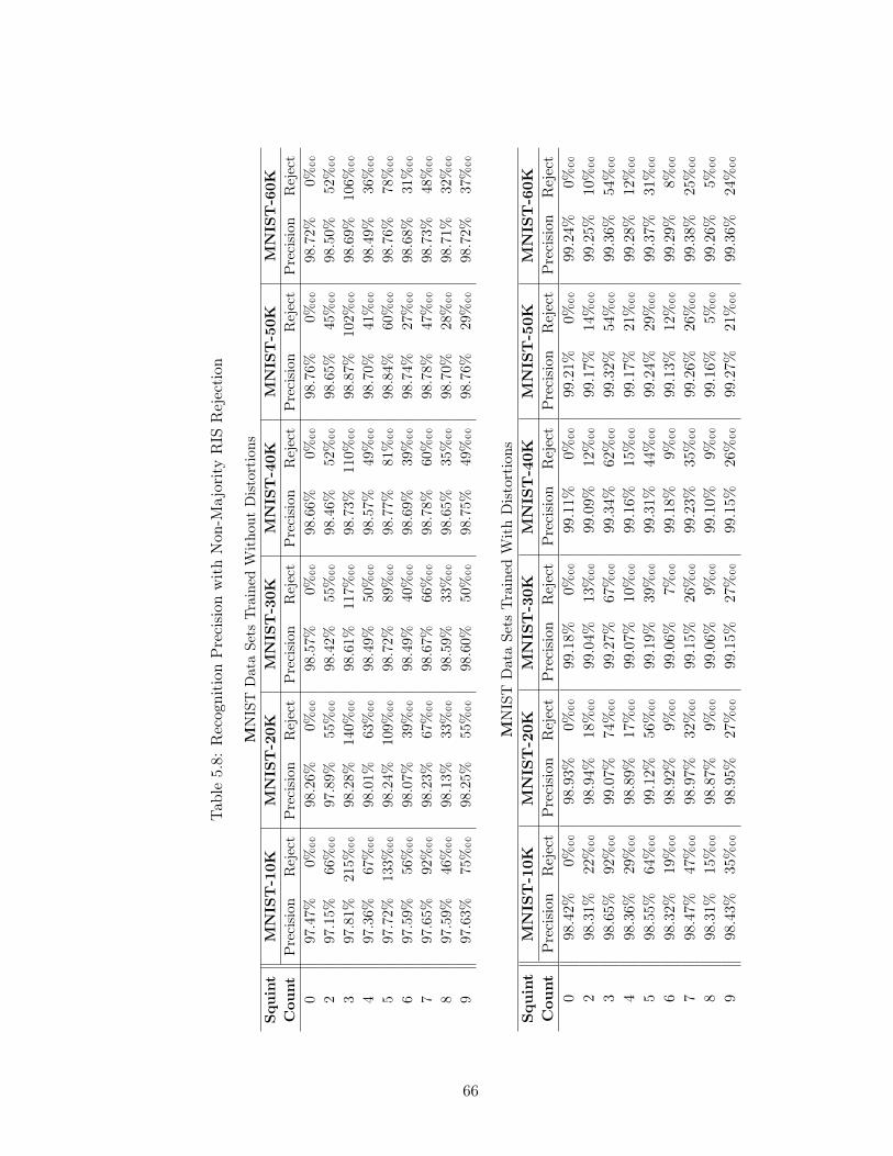
Tab

le5.

8:R

ecog

niti

onP

reci

sion

wit

hN

on-M

ajor

ity

RIS

Rej

ecti

on

MN

IST

Dat

aSe

tsTra

ined

Wit

hout

Dis

tort

ions

Squ

int

MN

IST

-10K

MN

IST

-20K

MN

IST

-30K

MN

IST

-40K

MN

IST

-50K

MN

IST

-60K

Cou

ntP

reci

sion

Rej

ect

Pre

cisi

onR

ejec

tP

reci

sion

Rej

ect

Pre

cisi

onR

ejec

tP

reci

sion

Rej

ect

Pre

cisi

onR

ejec

t0

97.4

7%0%

��98

.26%

0%��

98.5

7%0%

��98

.66%

0%��

98.7

6%0%

��98

.72%

0%��

297

.15%

66%

��97

.89%

55%

��98

.42%

55%

��98

.46%

52%

��98

.65%

45%

��98

.50%

52%

��3

97.8

1%21

5%��

98.2

8%14

0%��

98.6

1%11

7%��

98.7

3%11

0%��

98.8

7%10

2%��

98.6

9%10

6%��

497

.36%

67%

��98

.01%

63%

��98

.49%

50%

��98

.57%

49%

��98

.70%

41%

��98

.49%

36%

��5

97.7

2%13

3%��

98.2

4%10

9%��

98.7

2%89

%��

98.7

7%81

%��

98.8

4%60

%��

98.7

6%78

%��

697

.59%

56%

��98

.07%

39%

��98

.49%

40%

��98

.69%

39%

��98

.74%

27%

��98

.68%

31%

��7

97.6

5%92

%��

98.2

3%67

%��

98.6

7%66

%��

98.7

8%60

%��

98.7

8%47

%��

98.7

3%48

%��

897

.59%

46%

��98

.13%

33%

��98

.59%

33%

��98

.65%

35%

��98

.70%

28%

��98

.71%

32%

��9

97.6

3%75

%��

98.2

5%55

%��

98.6

0%50

%��

98.7

5%49

%��

98.7

6%29

%��

98.7

2%37

%��

MN

IST

Dat

aSe

tsTra

ined

Wit

hD

isto

rtio

nsSqu

int

MN

IST

-10K

MN

IST

-20K

MN

IST

-30K

MN

IST

-40K

MN

IST

-50K

MN

IST

-60K

Cou

ntP

reci

sion

Rej

ect

Pre

cisi

onR

ejec

tP

reci

sion

Rej

ect

Pre

cisi

onR

ejec

tP

reci

sion

Rej

ect

Pre

cisi

onR

ejec

t0

98.4

2%0%

��98

.93%

0%��

99.1

8%0%

��99

.11%

0%��

99.2

1%0%

��99

.24%

0%��

298

.31%

22%

��98

.94%

18%

��99

.04%

13%

��99

.09%

12%

��99

.17%

14%

��99

.25%

10%

��3

98.6

5%92

%��

99.0

7%74

%��

99.2

7%67

%��

99.3

4%62

%��

99.3

2%54

%��

99.3

6%54

%��

498

.36%

29%

��98

.89%

17%

��99

.07%

10%

��99

.16%

15%

��99

.17%

21%

��99

.28%

12%

��5

98.5

5%64

%��

99.1

2%56

%��

99.1

9%39

%��

99.3

1%44

%��

99.2

4%29

%��

99.3

7%31

%��

698

.32%

19%

��98

.92%

9%��

99.0

6%7%

��99

.18%

9%��

99.1

3%12

%��

99.2

9%8%

��7

98.4

7%47

%��

98.9

7%32

%��

99.1

5%26

%��

99.2

3%35

%��

99.2

6%26

%��

99.3

8%25

%��

898

.31%

15%

��98

.87%

9%��

99.0

6%9%

��99

.10%

9%��

99.1

6%5%

��99

.26%

5%��

998

.43%

35%

��98

.95%

27%

��99

.15%

27%

��99

.15%

26%

��99

.27%

21%

��99

.36%

24%

��

66

cases, the rejection curves follow a smooth and regular decline as the rejection rate is

decreased which demonstrates that this criterion is suitable for adjusting the rejection rate

with a predictable effect on precision. The second observation is that the rejection curves

become more smooth and regular as the fixed squint count is increased. This is most

pronounced in the cases involving MNIST models trained without distortions which are

depicted in Figure 5.11. This finding suggests that increasing the number of squints may

allow less rejections to be made while maintaining a relatively high rate of precision.

5.6 Experiments Generating ECOC Codes

The parameters for non-pruned codebook generation are: the desired codeword length

N , the codeword Hamming weight M and the minimum Hamming distance between code-

book codewords D. For the experiments conducted, the values of N were limited to odd

integers in the range [5, 47]; the values of M were limited to either M =N2

or M =

N2

as these choices guarantee a set of binary codewords with roughly the same number of

0’s and 1’s and since N is odd, the possibility of complementary codewords being gener-

ated is eliminated; the values of D were limited to odd integers generally within the range2 ·N4

− 3, 2 ·

N4

+ 1

for N ≥ 13 since this range was found to provide the maximum

error-correcting ability while still generating a useful number of candidate codewords in

most cases.

The experiments were carried out on a 2.93 GHz Intel Core 2 Duo processor and the

required computation time to exhaustively explore the search space for each set of tested

parameters is depicted in Figure 5.13. The exponential growth in the computation time as

N and D are increased is quite apparent as is the realization that this exhaustive approach

to codeword generation ceases to be practical for values of N > 48.

The number of codewords produced for each set of tested parameters are graphically

depicted in Figure 5.14 and a summary of these results is presented in Table 5.9.

67

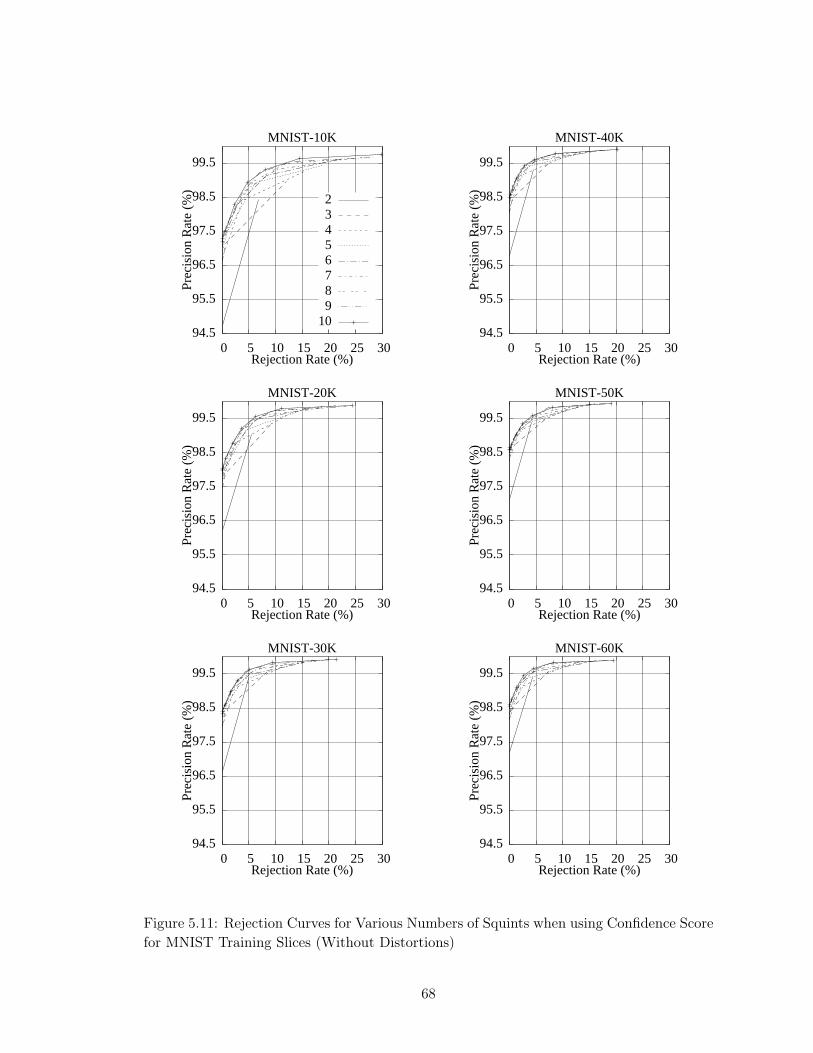
94.5

95.5

96.5

97.5

98.5

99.5

0 5 10 15 20 25 30

Prec

isio

n R

ate

(%)

Rejection Rate (%)

MNIST-10K

23456789

10

94.5

95.5

96.5

97.5

98.5

99.5

0 5 10 15 20 25 30

Prec

isio

n R

ate

(%)

Rejection Rate (%)

MNIST-20K

94.5

95.5

96.5

97.5

98.5

99.5

0 5 10 15 20 25 30

Prec

isio

n R

ate

(%)

Rejection Rate (%)

MNIST-30K

94.5

95.5

96.5

97.5

98.5

99.5

0 5 10 15 20 25 30

Prec

isio

n R

ate

(%)

Rejection Rate (%)

MNIST-40K

94.5

95.5

96.5

97.5

98.5

99.5

0 5 10 15 20 25 30

Prec

isio

n R

ate

(%)

Rejection Rate (%)

MNIST-50K

94.5

95.5

96.5

97.5

98.5

99.5

0 5 10 15 20 25 30

Prec

isio

n R

ate

(%)

Rejection Rate (%)

MNIST-60K

Figure 5.11: Rejection Curves for Various Numbers of Squints when using Confidence Scorefor MNIST Training Slices (Without Distortions)

68

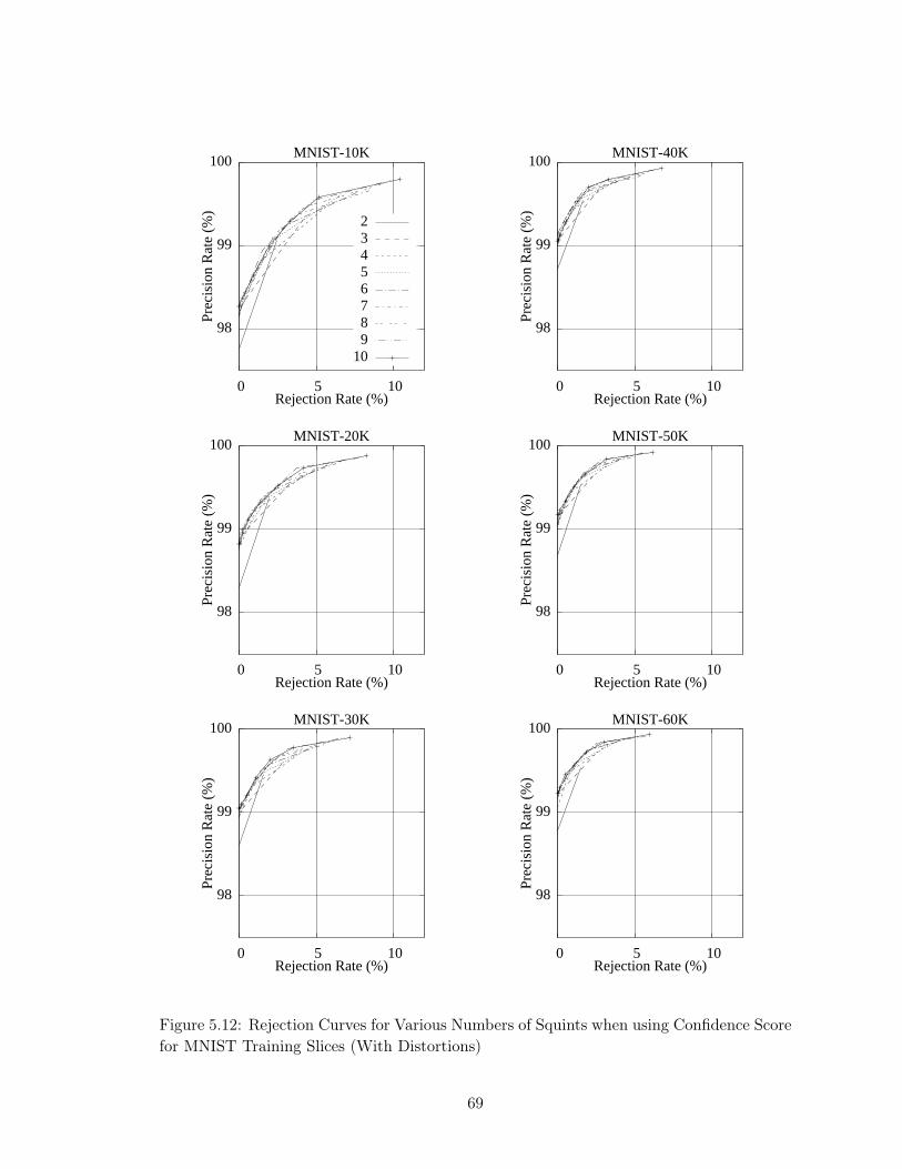
98

99

100

0 5 10

Prec

isio

n R

ate

(%)

Rejection Rate (%)

MNIST-10K

23456789

10

98

99

100

0 5 10

Prec

isio

n R

ate

(%)

Rejection Rate (%)

MNIST-20K

98

99

100

0 5 10

Prec

isio

n R

ate

(%)

Rejection Rate (%)

MNIST-30K

98

99

100

0 5 10

Prec

isio

n R

ate

(%)

Rejection Rate (%)

MNIST-40K

98

99

100

0 5 10

Prec

isio

n R

ate

(%)

Rejection Rate (%)

MNIST-50K

98

99

100

0 5 10

Prec

isio

n R

ate

(%)

Rejection Rate (%)

MNIST-60K

Figure 5.12: Rejection Curves for Various Numbers of Squints when using Confidence Scorefor MNIST Training Slices (With Distortions)

69

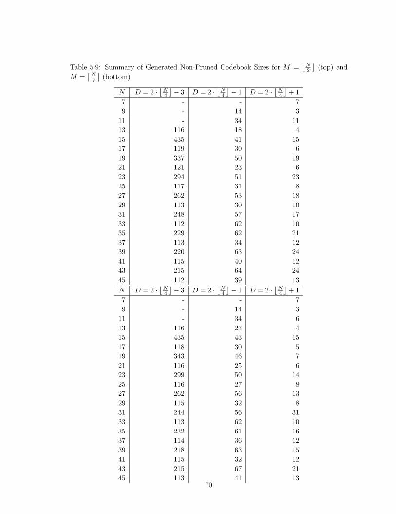
Table 5.9: Summary of Generated Non-Pruned Codebook Sizes for M =N2

(top) and

M =N2

(bottom)

N D = 2 ·N4

− 3 D = 2 ·

N4

− 1 D = 2 ·

N4

+ 1

7 - - 79 - 14 3

11 - 34 1113 116 18 415 435 41 1517 119 30 619 337 50 1921 121 23 623 294 51 2325 117 31 827 262 53 1829 113 30 1031 248 57 1733 112 62 1035 229 62 2137 113 34 1239 220 63 2441 115 40 1243 215 64 2445 112 39 13N D = 2 ·

N4

− 3 D = 2 ·

N4

− 1 D = 2 ·

N4

+ 1

7 - - 79 - 14 3

11 - 34 613 116 23 415 435 43 1517 118 30 519 343 46 721 116 25 623 299 50 1425 116 27 827 262 56 1329 115 32 831 244 56 3133 113 62 1035 232 61 1637 114 36 1239 218 63 1541 115 32 1243 215 67 2145 113 41 13

70

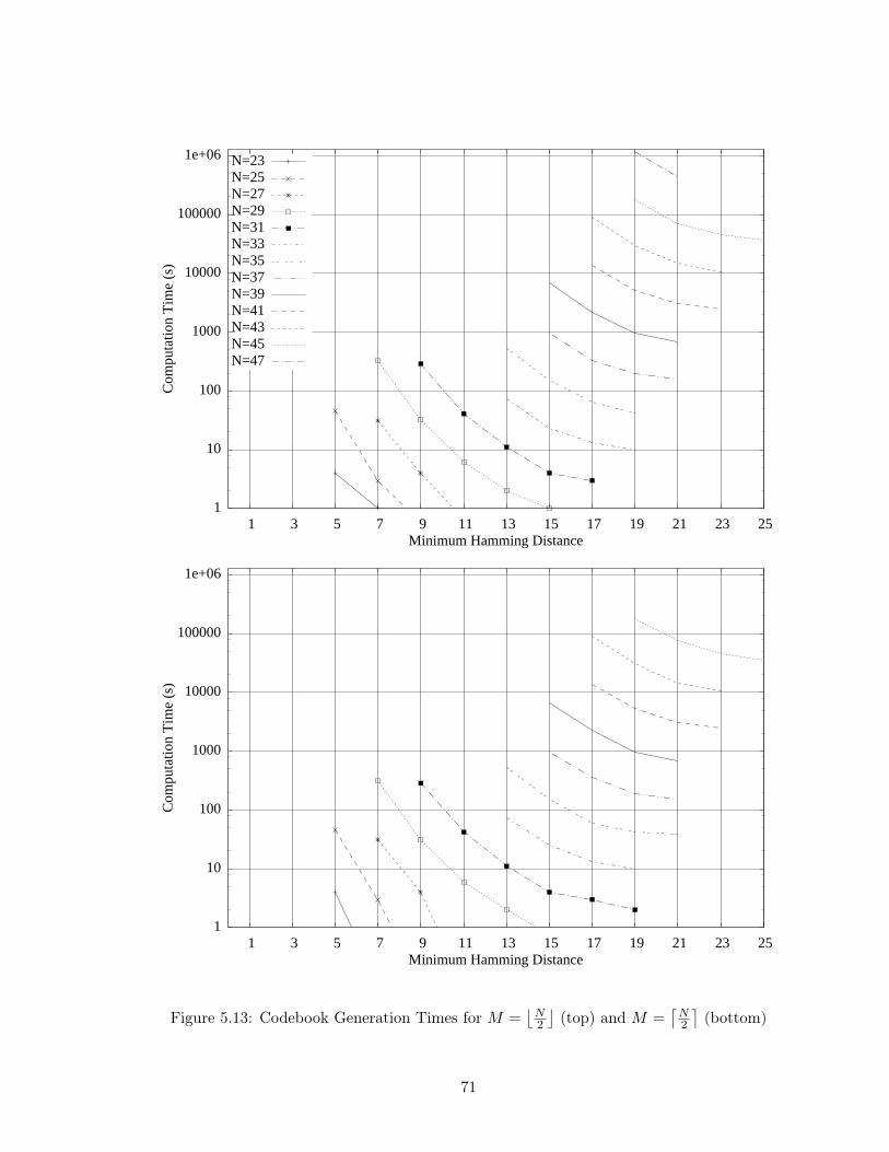
1

10

100

1000

10000

100000

1e+06

1 3 5 7 9 11 13 15 17 19 21 23 25

Com

puta

tion

Tim

e (s

)

Minimum Hamming Distance

N=23N=25N=27N=29N=31N=33N=35N=37N=39N=41N=43N=45N=47

1

10

100

1000

10000

100000

1e+06

1 3 5 7 9 11 13 15 17 19 21 23 25

Com

puta

tion

Tim

e (s

)

Minimum Hamming Distance

Figure 5.13: Codebook Generation Times for M =N2

(top) and M =

N2

(bottom)

71

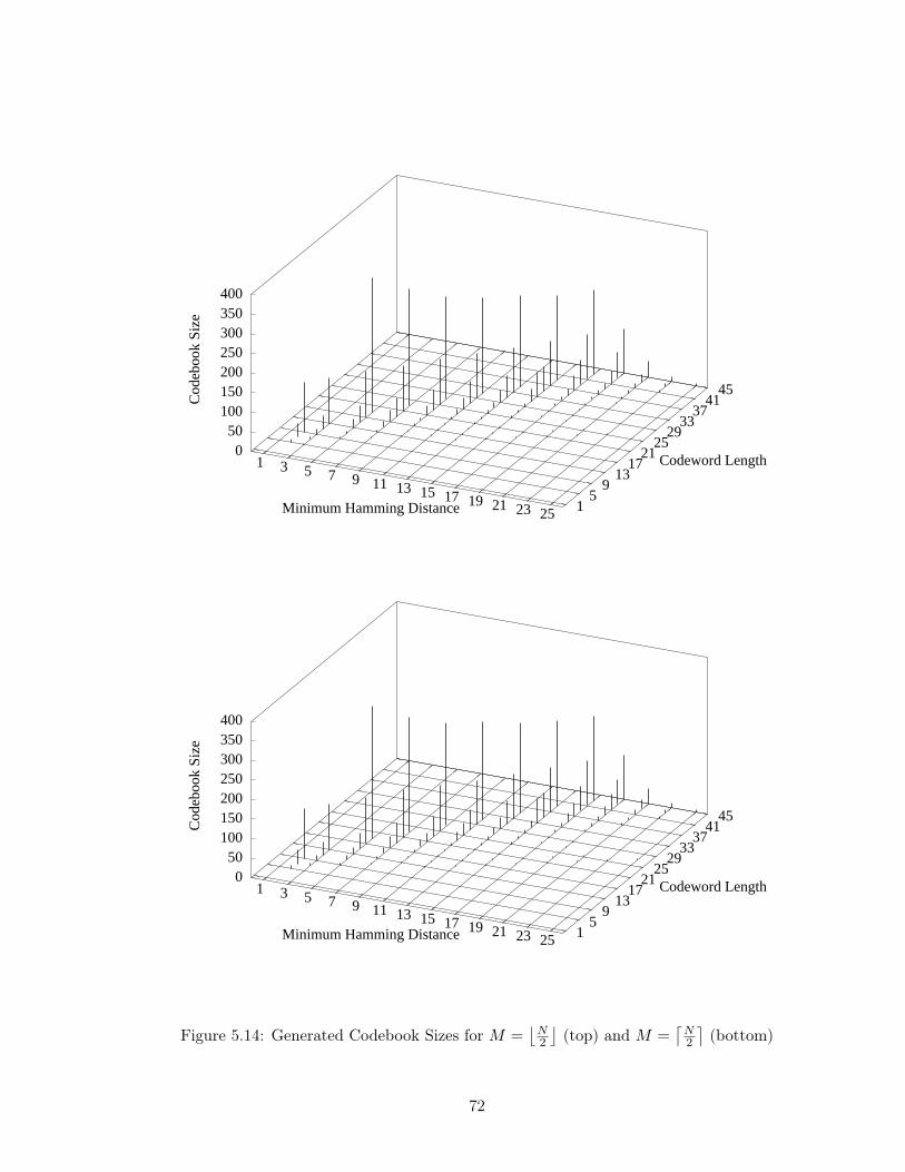
1 3 5 7 9 11 13 15 17 19 21 23 25Minimum Hamming Distance 1 5

9 13

17 21

25 29

33 37

41 45

Codeword Length 0

50 100 150 200 250 300 350 400

Cod

eboo

k Si

ze

1 3 5 7 9 11 13 15 17 19 21 23 25Minimum Hamming Distance 1 5

9 13

17 21

25 29

33 37

41 45

Codeword Length 0

50 100 150 200 250 300 350 400

Cod

eboo

k Si

ze

Figure 5.14: Generated Codebook Sizes for M =N2

(top) and M =

N2

(bottom)

72

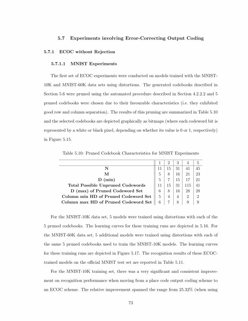
5.7 Experiments involving Error-Correcting Output Coding

5.7.1 ECOC without Rejection

5.7.1.1 MNIST Experiments

The first set of ECOC experiments were conducted on models trained with the MNIST-

10K and MNIST-60K data sets using distortions. The generated codebooks described in

Section 5.6 were pruned using the automated procedure described in Section 4.2.2.2 and 5

pruned codebooks were chosen due to their favourable characteristics (i.e. they exhibited

good row and column separation). The results of this pruning are summarized in Table 5.10

and the selected codebooks are depicted graphically as bitmaps (where each codeword bit is

represented by a white or black pixel, depending on whether its value is 0 or 1, respectively)

in Figure 5.15.

Table 5.10: Pruned Codebook Characteristics for MNIST Experiments

1 2 3 4 5N 11 15 31 41 45M 5 8 16 21 23

D (min) 5 7 15 17 21Total Possible Unpruned Codewords 11 15 31 115 41D (max) of Pruned Codeword Set 6 8 16 28 28

Column min HD of Pruned Codeword Set 5 4 4 2 2Column max HD of Pruned Codeword Set 6 7 8 9 9

For the MNIST-10K data set, 5 models were trained using distortions with each of the

5 pruned codebooks. The learning curves for these training runs are depicted in 5.16. For

the MNIST-60K data set, 5 additional models were trained using distortions with each of

the same 5 pruned codebooks used to train the MNIST-10K models. The learning curves

for these training runs are depicted in Figure 5.17. The recognition results of these ECOC-

trained models on the official MNIST test set are reported in Table 5.11.

For the MNIST-10K training set, there was a very significant and consistent improve-

ment on recognition performance when moving from a place code output coding scheme to

an ECOC scheme. The relative improvement spanned the range from 25.32% (when using

73

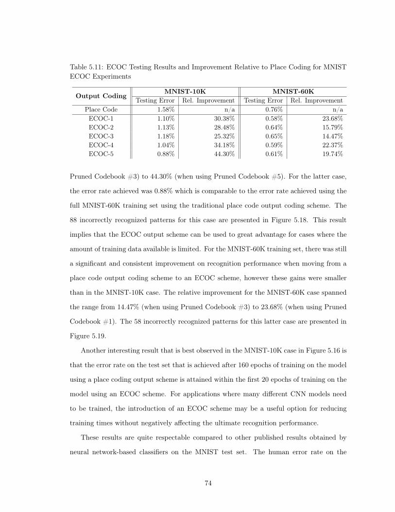
Table 5.11: ECOC Testing Results and Improvement Relative to Place Coding for MNISTECOC Experiments

Output CodingMNIST-10K MNIST-60K

Testing Error Rel. Improvement Testing Error Rel. ImprovementPlace Code 1.58% n/a 0.76% n/aECOC-1 1.10% 30.38% 0.58% 23.68%ECOC-2 1.13% 28.48% 0.64% 15.79%ECOC-3 1.18% 25.32% 0.65% 14.47%ECOC-4 1.04% 34.18% 0.59% 22.37%ECOC-5 0.88% 44.30% 0.61% 19.74%

Pruned Codebook #3) to 44.30% (when using Pruned Codebook #5). For the latter case,

the error rate achieved was 0.88% which is comparable to the error rate achieved using the

full MNIST-60K training set using the traditional place code output coding scheme. The

88 incorrectly recognized patterns for this case are presented in Figure 5.18. This result

implies that the ECOC output scheme can be used to great advantage for cases where the

amount of training data available is limited. For the MNIST-60K training set, there was still

a significant and consistent improvement on recognition performance when moving from a

place code output coding scheme to an ECOC scheme, however these gains were smaller

than in the MNIST-10K case. The relative improvement for the MNIST-60K case spanned

the range from 14.47% (when using Pruned Codebook #3) to 23.68% (when using Pruned

Codebook #1). The 58 incorrectly recognized patterns for this latter case are presented in

Figure 5.19.

Another interesting result that is best observed in the MNIST-10K case in Figure 5.16 is

that the error rate on the test set that is achieved after 160 epochs of training on the model

using a place coding output scheme is attained within the first 20 epochs of training on the

model using an ECOC scheme. For applications where many different CNN models need

to be trained, the introduction of an ECOC scheme may be a useful option for reducing

training times without negatively affecting the ultimate recognition performance.

These results are quite respectable compared to other published results obtained by

neural network-based classifiers on the MNIST test set. The human error rate on the

74

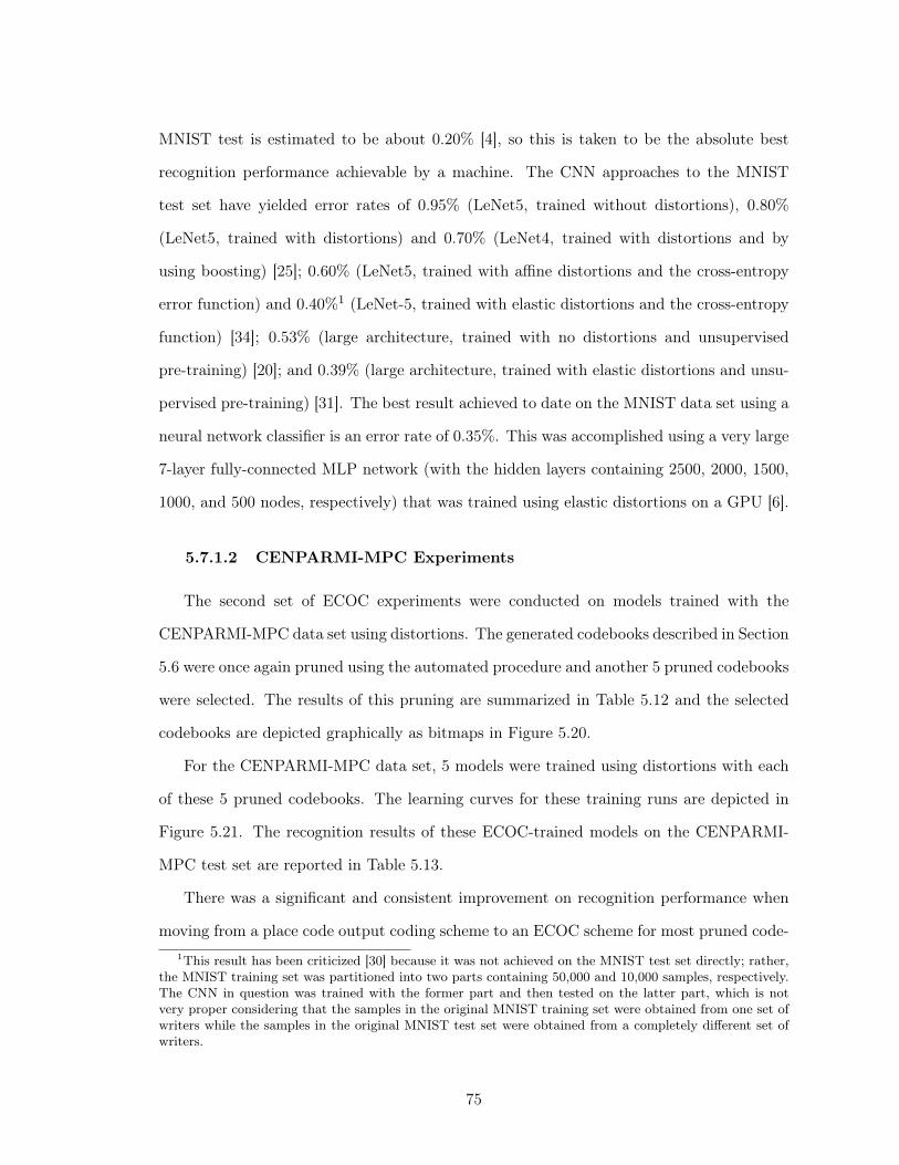
MNIST test is estimated to be about 0.20% [4], so this is taken to be the absolute best

recognition performance achievable by a machine. The CNN approaches to the MNIST

test set have yielded error rates of 0.95% (LeNet5, trained without distortions), 0.80%

(LeNet5, trained with distortions) and 0.70% (LeNet4, trained with distortions and by

using boosting) [25]; 0.60% (LeNet5, trained with affine distortions and the cross-entropy

error function) and 0.40%1 (LeNet-5, trained with elastic distortions and the cross-entropy

function) [34]; 0.53% (large architecture, trained with no distortions and unsupervised

pre-training) [20]; and 0.39% (large architecture, trained with elastic distortions and unsu-

pervised pre-training) [31]. The best result achieved to date on the MNIST data set using a

neural network classifier is an error rate of 0.35%. This was accomplished using a very large

7-layer fully-connected MLP network (with the hidden layers containing 2500, 2000, 1500,

1000, and 500 nodes, respectively) that was trained using elastic distortions on a GPU [6].

5.7.1.2 CENPARMI-MPC Experiments

The second set of ECOC experiments were conducted on models trained with the

CENPARMI-MPC data set using distortions. The generated codebooks described in Section

5.6 were once again pruned using the automated procedure and another 5 pruned codebooks

were selected. The results of this pruning are summarized in Table 5.12 and the selected

codebooks are depicted graphically as bitmaps in Figure 5.20.

For the CENPARMI-MPC data set, 5 models were trained using distortions with each

of these 5 pruned codebooks. The learning curves for these training runs are depicted in

Figure 5.21. The recognition results of these ECOC-trained models on the CENPARMI-

MPC test set are reported in Table 5.13.

There was a significant and consistent improvement on recognition performance when

moving from a place code output coding scheme to an ECOC scheme for most pruned code-1This result has been criticized [30] because it was not achieved on the MNIST test set directly; rather,

the MNIST training set was partitioned into two parts containing 50,000 and 10,000 samples, respectively.The CNN in question was trained with the former part and then tested on the latter part, which is notvery proper considering that the samples in the original MNIST training set were obtained from one set ofwriters while the samples in the original MNIST test set were obtained from a completely different set ofwriters.

75

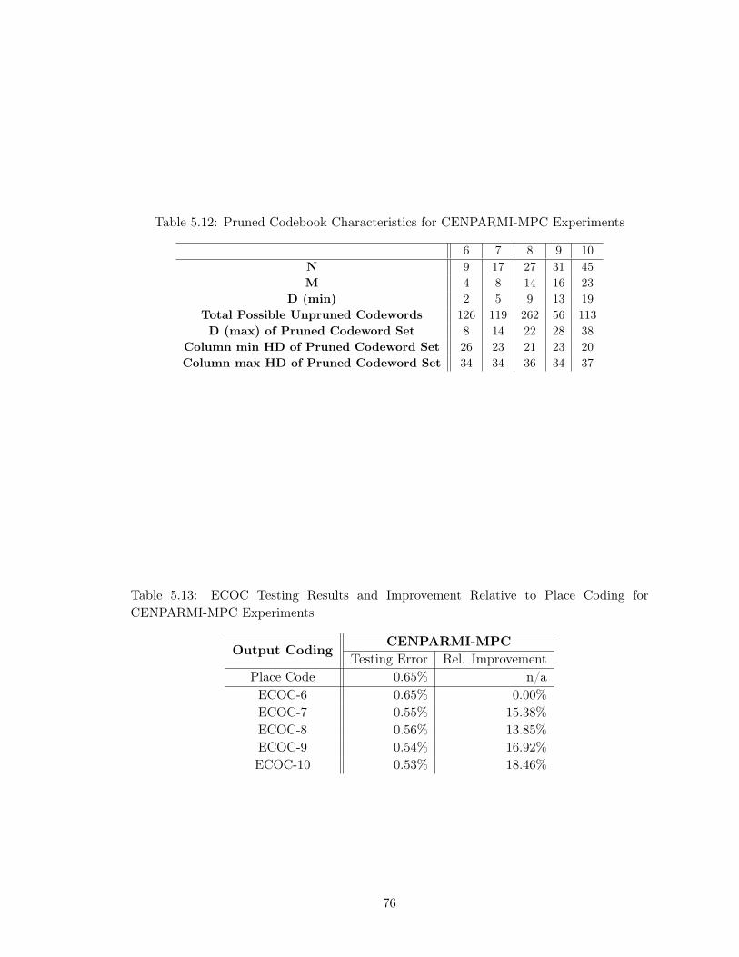
Table 5.12: Pruned Codebook Characteristics for CENPARMI-MPC Experiments

6 7 8 9 10N 9 17 27 31 45M 4 8 14 16 23

D (min) 2 5 9 13 19Total Possible Unpruned Codewords 126 119 262 56 113D (max) of Pruned Codeword Set 8 14 22 28 38

Column min HD of Pruned Codeword Set 26 23 21 23 20Column max HD of Pruned Codeword Set 34 34 36 34 37

Table 5.13: ECOC Testing Results and Improvement Relative to Place Coding forCENPARMI-MPC Experiments

Output CodingCENPARMI-MPC

Testing Error Rel. ImprovementPlace Code 0.65% n/aECOC-6 0.65% 0.00%ECOC-7 0.55% 15.38%ECOC-8 0.56% 13.85%ECOC-9 0.54% 16.92%ECOC-10 0.53% 18.46%

76

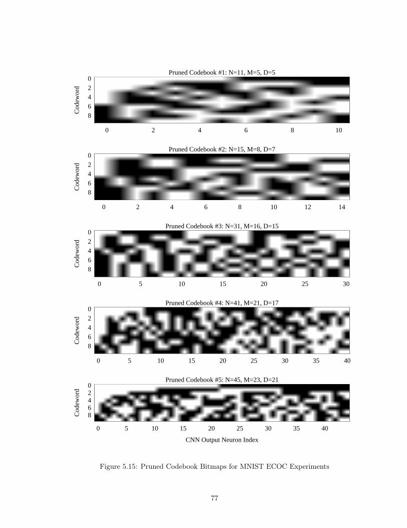
0 2 4 6 8

0 2 4 6 8 10

Cod

ewor

dPruned Codebook #1: N=11, M=5, D=5

0 2 4 6 8

0 2 4 6 8 10 12 14

Cod

ewor

d

Pruned Codebook #2: N=15, M=8, D=7

0 2 4 6 8

0 5 10 15 20 25 30

Cod

ewor

d

Pruned Codebook #3: N=31, M=16, D=15

0 2 4 6 8

0 5 10 15 20 25 30 35 40

Cod

ewor

d

Pruned Codebook #4: N=41, M=21, D=17

0 2 4 6 8

0 5 10 15 20 25 30 35 40

Cod

ewor

d

CNN Output Neuron Index

Pruned Codebook #5: N=45, M=23, D=21

Figure 5.15: Pruned Codebook Bitmaps for MNIST ECOC Experiments

77

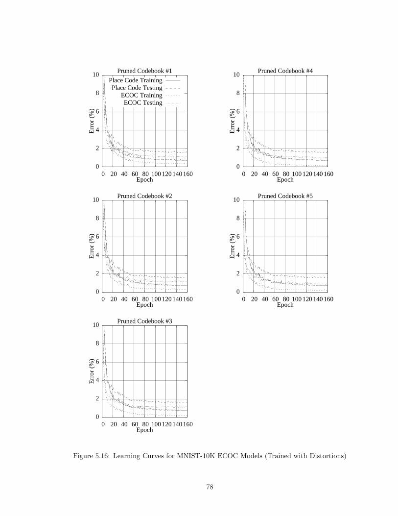
0

2

4

6

8

10

0 20 40 60 80 100 120 140 160

Erro

r (%

)

Epoch

Pruned Codebook #1Place Code TrainingPlace Code Testing

ECOC TrainingECOC Testing

0

2

4

6

8

10

0 20 40 60 80 100 120 140 160

Erro

r (%

)

Epoch

Pruned Codebook #2

0

2

4

6

8

10

0 20 40 60 80 100 120 140 160

Erro

r (%

)

Epoch

Pruned Codebook #3

0

2

4

6

8

10

0 20 40 60 80 100 120 140 160

Erro

r (%

)

Epoch

Pruned Codebook #4

0

2

4

6

8

10

0 20 40 60 80 100 120 140 160

Erro

r (%

)

Epoch

Pruned Codebook #5

Figure 5.16: Learning Curves for MNIST-10K ECOC Models (Trained with Distortions)

78

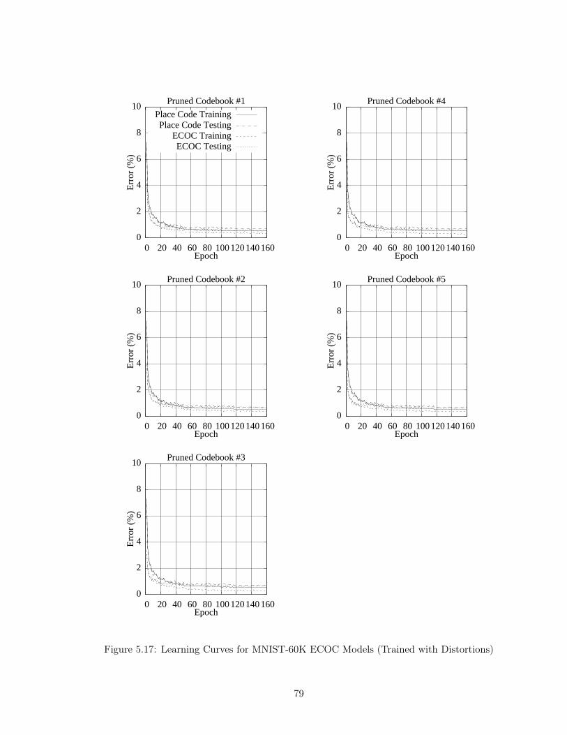
0

2

4

6

8

10

0 20 40 60 80 100 120 140 160

Erro

r (%

)

Epoch

Pruned Codebook #1Place Code TrainingPlace Code Testing

ECOC TrainingECOC Testing

0

2

4

6

8

10

0 20 40 60 80 100 120 140 160

Erro

r (%

)

Epoch

Pruned Codebook #2

0

2

4

6

8

10

0 20 40 60 80 100 120 140 160

Erro

r (%

)

Epoch

Pruned Codebook #3

0

2

4

6

8

10

0 20 40 60 80 100 120 140 160

Erro

r (%

)

Epoch

Pruned Codebook #4

0

2

4

6

8

10

0 20 40 60 80 100 120 140 160

Erro

r (%

)

Epoch

Pruned Codebook #5

Figure 5.17: Learning Curves for MNIST-60K ECOC Models (Trained with Distortions)

79

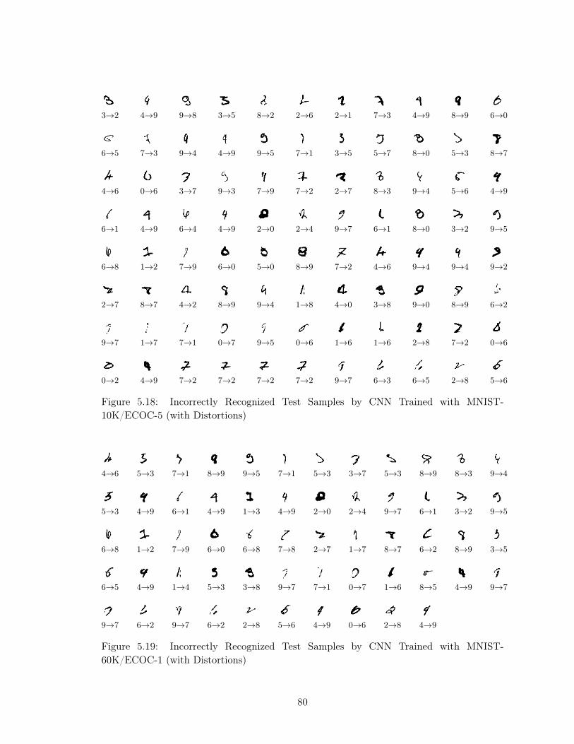
3→2 4→9 9→8 3→5 8→2 2→6 2→1 7→3 4→9 8→9 6→0

6→5 7→3 9→4 4→9 9→5 7→1 3→5 5→7 8→0 5→3 8→7

4→6 0→6 3→7 9→3 7→9 7→2 2→7 8→3 9→4 5→6 4→9

6→1 4→9 6→4 4→9 2→0 2→4 9→7 6→1 8→0 3→2 9→5

6→8 1→2 7→9 6→0 5→0 8→9 7→2 4→6 9→4 9→4 9→2

2→7 8→7 4→2 8→9 9→4 1→8 4→0 3→8 9→0 8→9 6→2

9→7 1→7 7→1 0→7 9→5 0→6 1→6 1→6 2→8 7→2 0→6

0→2 4→9 7→2 7→2 7→2 7→2 9→7 6→3 6→5 2→8 5→6

Figure 5.18: Incorrectly Recognized Test Samples by CNN Trained with MNIST-10K/ECOC-5 (with Distortions)

4→6 5→3 7→1 8→9 9→5 7→1 5→3 3→7 5→3 8→9 8→3 9→4

5→3 4→9 6→1 4→9 1→3 4→9 2→0 2→4 9→7 6→1 3→2 9→5

6→8 1→2 7→9 6→0 6→8 7→8 2→7 1→7 8→7 6→2 8→9 3→5

6→5 4→9 1→4 5→3 3→8 9→7 7→1 0→7 1→6 8→5 4→9 9→7

9→7 6→2 9→7 6→2 2→8 5→6 4→9 0→6 2→8 4→9

Figure 5.19: Incorrectly Recognized Test Samples by CNN Trained with MNIST-60K/ECOC-1 (with Distortions)

80

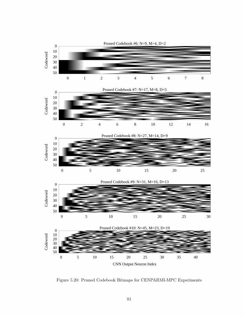
0 10 20 30 40 50

0 1 2 3 4 5 6 7 8

Cod

ewor

dPruned Codebook #6: N=9, M=4, D=2

0 10 20 30 40 50

0 2 4 6 8 10 12 14 16

Cod

ewor

d

Pruned Codebook #7: N=17, M=8, D=5

0 10 20 30 40 50

0 5 10 15 20 25

Cod

ewor

d

Pruned Codebook #8: N=27, M=14, D=9

0 10 20 30 40 50

0 5 10 15 20 25 30

Cod

ewor

d

Pruned Codebook #9: N=31, M=16, D=13

0 10 20 30 40 50

0 5 10 15 20 25 30 35 40

Cod

ewor

d

CNN Output Neuron Index

Pruned Codebook #10: N=45, M=23, D=19

Figure 5.20: Pruned Codebook Bitmaps for CENPARMI-MPC Experiments

81

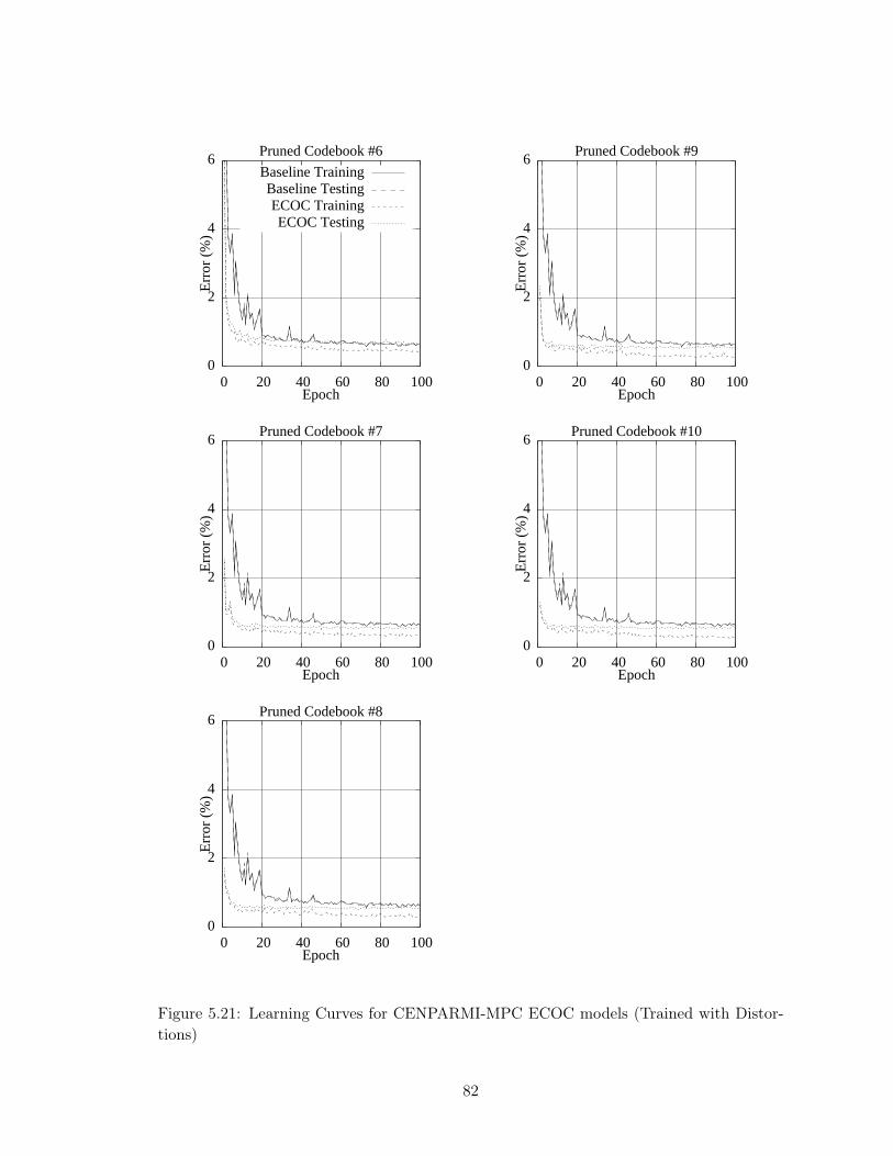
0

2

4

6

0 20 40 60 80 100

Erro

r (%

)

Epoch

Pruned Codebook #6Baseline TrainingBaseline TestingECOC TrainingECOC Testing

0

2

4

6

0 20 40 60 80 100

Erro

r (%

)

Epoch

Pruned Codebook #7

0

2

4

6

0 20 40 60 80 100

Erro

r (%

)

Epoch

Pruned Codebook #8

0

2

4

6

0 20 40 60 80 100

Erro

r (%

)

Epoch

Pruned Codebook #9

0

2

4

6

0 20 40 60 80 100

Erro

r (%

)

Epoch

Pruned Codebook #10

Figure 5.21: Learning Curves for CENPARMI-MPC ECOC models (Trained with Distor-tions)

82

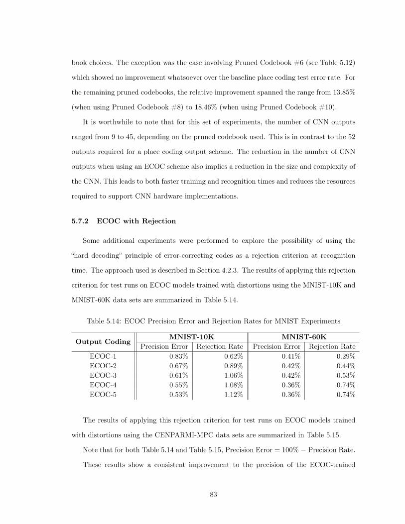
book choices. The exception was the case involving Pruned Codebook #6 (see Table 5.12)

which showed no improvement whatsoever over the baseline place coding test error rate. For

the remaining pruned codebooks, the relative improvement spanned the range from 13.85%

(when using Pruned Codebook #8) to 18.46% (when using Pruned Codebook #10).

It is worthwhile to note that for this set of experiments, the number of CNN outputs

ranged from 9 to 45, depending on the pruned codebook used. This is in contrast to the 52

outputs required for a place coding output scheme. The reduction in the number of CNN

outputs when using an ECOC scheme also implies a reduction in the size and complexity of

the CNN. This leads to both faster training and recognition times and reduces the resources

required to support CNN hardware implementations.

5.7.2 ECOC with Rejection

Some additional experiments were performed to explore the possibility of using the

“hard decoding” principle of error-correcting codes as a rejection criterion at recognition

time. The approach used is described in Section 4.2.3. The results of applying this rejection

criterion for test runs on ECOC models trained with distortions using the MNIST-10K and

MNIST-60K data sets are summarized in Table 5.14.

Table 5.14: ECOC Precision Error and Rejection Rates for MNIST Experiments

Output CodingMNIST-10K MNIST-60K

Precision Error Rejection Rate Precision Error Rejection RateECOC-1 0.83% 0.62% 0.41% 0.29%ECOC-2 0.67% 0.89% 0.42% 0.44%ECOC-3 0.61% 1.06% 0.42% 0.53%ECOC-4 0.55% 1.08% 0.36% 0.74%ECOC-5 0.53% 1.12% 0.36% 0.74%

The results of applying this rejection criterion for test runs on ECOC models trained

with distortions using the CENPARMI-MPC data sets are summarized in Table 5.15.

Note that for both Table 5.14 and Table 5.15, Precision Error = 100% − Precision Rate.

These results show a consistent improvement to the precision of the ECOC-trained

83

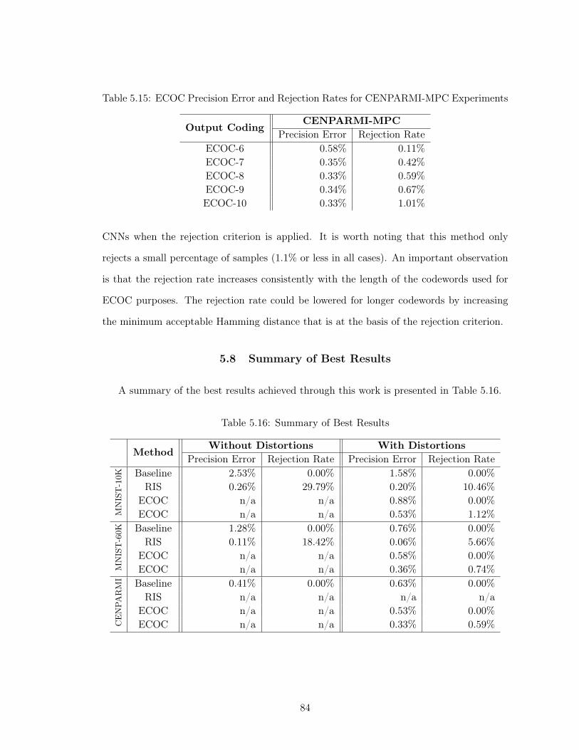
Table 5.15: ECOC Precision Error and Rejection Rates for CENPARMI-MPC Experiments

Output CodingCENPARMI-MPC

Precision Error Rejection RateECOC-6 0.58% 0.11%ECOC-7 0.35% 0.42%ECOC-8 0.33% 0.59%ECOC-9 0.34% 0.67%ECOC-10 0.33% 1.01%

CNNs when the rejection criterion is applied. It is worth noting that this method only

rejects a small percentage of samples (1.1% or less in all cases). An important observation

is that the rejection rate increases consistently with the length of the codewords used for

ECOC purposes. The rejection rate could be lowered for longer codewords by increasing

the minimum acceptable Hamming distance that is at the basis of the rejection criterion.

5.8 Summary of Best Results

A summary of the best results achieved through this work is presented in Table 5.16.

Table 5.16: Summary of Best Results

MethodWithout Distortions With Distortions

Precision Error Rejection Rate Precision Error Rejection Rate

MN

IST

-10K Baseline 2.53% 0.00% 1.58% 0.00%

RIS 0.26% 29.79% 0.20% 10.46%ECOC n/a n/a 0.88% 0.00%ECOC n/a n/a 0.53% 1.12%

MN

IST

-60K Baseline 1.28% 0.00% 0.76% 0.00%

RIS 0.11% 18.42% 0.06% 5.66%ECOC n/a n/a 0.58% 0.00%ECOC n/a n/a 0.36% 0.74%

CE

NPA

RM

I Baseline 0.41% 0.00% 0.63% 0.00%RIS n/a n/a n/a n/a

ECOC n/a n/a 0.53% 0.00%ECOC n/a n/a 0.33% 0.59%

84

CHAPTER 6. CONCLUSIONS

This thesis examined the question of improving Convolutional Neural Network (CNN)

performance when the quantity of training data is limited. Two techniques, Recognition

Input Squinting (RIS) and Error-Correcting Output Coding (ECOC), were implemented

as enhancements to a standard CNN implementation and experiments were conducted to

evaluate the results of these methods on two data sets containing character images. One of

the appealing aspects of these techniques is that they can be added relatively easily to an

existing CNN recognition system.

6.1 Contributions

The main contributions of this thesis are:

1. Introduction of a novel confidence metric based on RIS designed specifically for CNNs,

that can be used as part of a rejection strategy for dubiously-recognized patterns,

particularly in cases where the training data set is small;

2. Confirmation that the ECOC technique can be used to improve CNN recognition

precision;

3. Creation of an efficient exhaustive search routine for finding suitable ECOC candidates

up to 48-bits in length; and

4. Generation of several codebooks suitable for use in CNN ECOC and other application

areas.

85

6.2 Future Work

There are several unanswered questions that have been raised through this work that

could be further explored in the future.

On the RIS front, this work dealt with the generation of squinted images using random

parameters. It would be useful to understand which types of image transformation are the

most effective for improving the rejection criterion and to come up with efficient methods

for optimizing the choice of transformation parameters. A general concern is the discovery

that certain patterns that are correctly classified by a standard CNN, fail to be recognized

correctly when subjected to random squinting over and over again. This seems to suggest

that a certain number of patterns that are correctly classified by the CNN are “accidents”

in the sense that the CNN has not made the decision due to successful generalization. As

such, these “accidents” inflate the reported testing error rates and misrepresent the true

generalization power of the network (which is precisely what the testing error is supposed

to indicate). The RIS procedure or some related variant could be employed as a more

realistic measure of a machine learning method’s generalization power.

On the ECOC front, it would be interesting to see the effect of exploiting prior infor-

mation about classes (e.g. which pairs of classes are typically confused) when assigning

codewords to classes. This would better ensure that the error-correcting power of the code

is directed to where it is most needed, in spite of early results [9] that suggest mapping

choice is immaterial to recognition performance. It would also be useful to understand how

well ECOC performance scales with the number of classes to be recognized and the effect

of codeword length on ECOC performance as the number of classes is increased.

Finally, since both the RIS and ECOC methods have been demonstrated in isolation to

raise CNN performance, experiments could be performed that combine these two methods

for even greater performance gains.

86

BIBLIOGRAPHY

[1] A. Abdulkader. Two-tier approach for arabic offline handwriting recognition. In

Proceedings of the 10th International Workshop on Frontiers in Handwriting Recog-

nition, pages 42–47, La Baule, France, October 2006.

[2] S. E. Anderson. Bit twiddling hacks. Last accessed: March 1, 2011.

http://graphics.stanford.edu/∼seander/bithacks.html#NextBitPermutation.

[3] Y. Bengio and X. Glorot. Understanding the difficulty of training deep feedforward

neural networks. In Proceedings of the 13th International Conference on Artificial

Intelligence and Statistics, volume 9, pages 249–256, Sardinia, Italy, May 2010.

[4] L. Bottou, C. Cortes, J. S. Denker, H. Drucker, I. Guyon, L. D. Jackel, Y. LeCun, U. A.

Muller, E. Sackinger, P. Simard, and V. Vapnik. Comparison of classifier methods:

a case study in handwritten digit recognition. In Proceedings of the International

Conference on Pattern Recognition, volume 2, pages 77–82, Jerusalem, Israel, October

1994.

[5] Y. Chen, C. Han, C. Wang, B. Jeng, and K. Fan. The application of a convolution

neural network on face and license plate detection. In Proceedings of the 18th Inter-

national Conference on Pattern Recognition, volume 3, pages 552–555, Hong Kong,

China, 2006.

[6] D. Ciresan, U. Meier, L. Gambardella, and J. Schmidhuber. Deep, big, simple neural

nets for handwritten digit recognition. Neural Computation, 22(12):3207–3220, 2010.

87

[7] H. Deng, G. Stathopoulos, and C. Y. Suen. Error-correcting output coding for the

convolutional neural network for optical character recognition. In Proceedings of the

10th International Conference on Document Analysis and Recognition, pages 581–585,

Barcelona, Spain, July 2009.

[8] H. Deng, G. Stathopoulos, and C. Y. Suen. Applying error-correcting output coding to

enhance convolutional neural network for target detection and pattern recognition. In

Proceedings of the 20th International Conference on Pattern Recognition, pages 4291–

4294, Istanbul, Turkey, August 2010.

[9] T. G. Dietterich and G. Bakiri. Solving multiclass learning problems via error-

correcting output codes. Journal of Artificial Intelligence Research, 2:263–286, 1995.

[10] H. Dietz. The aggregate magic algorithms. Last accessed: March 1, 2011.

http://aggregate.org/MAGIC/.

[11] R. O. Duda, P. E. Hart, and D. G. Stork. Pattern Classification. Wiley, New York,

2nd edition, 2001.

[12] Free Software Foundation. The GNU multiple precision arithmetic library.

Last accessed: March 1, 2011. http://gmplib.org/manual/Integer-Logic-and-Bit-

Fiddling.html#Integer-Logic-and-Bit-Fiddling.

[13] K. Fukushima and S. Miyake. Neocognitron: A new algorithm for pattern recognition

tolerant of deformations and shifts in position. Pattern Recognition, 15(6):455–469,

1982.

[14] C. Garcia and M. Delakis. Convolutional face finder: a neural architecture for fast and

robust face detection. IEEE Transactions on Pattern Analysis and Machine Intelli-

gence, 26(11):1408–1423, 2004.

[15] J. J. Gibson. The visual perception of objective motion and subjective movement.

Psychological Review, 61(5):304–314, 1954.

88

[16] J. J. Gibson. Optical motions and transformations as stimuli for visual perception.

Psychological Review, 64(5):288–295, 1957.

[17] J. J. Gibson. The senses considered as perceptual systems. Houghton Mifflin, Boston,

1966.

[18] R. Hadsell, P. Sermanet, M. Scoffier, A. Erkan, K. Kavackuoglu, U. Muller, and

Y. LeCun. Learning long-range vision for autonomous off-road driving. Journal of

Field Robotics, 26(2):120–144, 2009.

[19] D. H. Hubel and T. N. Wiesel. Receptive fields, binocular interaction and functional

architecture in the cat’s visual cortex. Journal of Physiology (London), 160:106–154,

1962.

[20] K. Jarrett, K. Kavukcuoglu, M. Ranzato, and Y. LeCun. What is the best multi-

stage architecture for object recognition? In Proceedings of the 12th International

Conference on Computer Vision, pages 2146–2153, Kyoto, Japan, September 2009.

[21] Ishtiaq Khan. Convolutional neural networks for recognition of handwritten digits.

Last accessed: May 1, 2008. http://www1.i2r.a-star.edu.sg/∼irkhan/conn1.html.

[22] F. Lauer, C. Y. Suen, and G. Bloch. A trainable feature extractor for handwritten

digit recognition. Pattern Recognition, 40:1816–1824, 2007.

[23] Y. LeCun. MNIST database of handwritten digits. Last accessed: March 1, 2011.

http://yann.lecun.com/exdb/mnist/.

[24] Y. LeCun, B. Boser, J. S. Denker, D. Henderson, R. E. Howard, W. Hubbard, and

L. D. Jackel. Backpropagation applied to handwritten zip code recognition. Neural

Computation, 1(4):541–551, Winter 1989.

[25] Y. Lecun, L. Bottou, Y. Bengio, and P. Haffner. Gradient-based learning applied to

document recognition. In Proceedings of the IEEE, volume 86(11), pages 2278–2324,

1998.

89

[26] Y. LeCun, F. Huang, and L. Bottou. Learning methods for generic object recognition

with invariance to pose and lighting. In Proceedings of the IEEE International Confer-

ence on Computer Vision and Pattern Recognition, pages 97–104, Washington, DC,

USA, June 2004.

[27] Y. Lecun, K. Kavukcuoglu, and C. Farabet. Convolutional networks and applications in

vision. In Proceedings of the IEEE International Symposium on Circuits and Systems,

pages 253–256, Paris, France, 2010.

[28] H. Lee, R. Grosse, R. Ranganath, and A. Y. Ng. Convolutional deep belief networks

for scalable unsupervised learning of hierarchical representations. In Proceedings of the

26th International Conference on Machine Learning, pages 609–616, Montreal, Quebec,

Canada, June 2009.

[29] W. S. McCulloch and W. Pitts. A logical calculus of the ideas immanent in nervous

activity. Bull. Mathematical Biophysics, 7:115–133, 1943.

[30] M. O’Neil. Neural network recognition of handwritten digits. Last accessed: March 1,

2011. http://www.codeproject.com/KB/library/NeuralNetRecognition.aspx.

[31] M. Ranzato, C. Poultney, S. Chopra, and Y. LeCun. Efficient learning of sparse repre-

sentations with an energy-based model. In Proceedings of the 20th Annual Conference

on Neural Information Processing Systems, pages 1137–1144, Vancouver, BC, Canada,

December 2006.

[32] F. Rosenblatt. The Perceptron: A Probabilistic Model for Information Storage and

Organization in the Brain. Psychological Review, 65(6):386–408, 1958.

[33] D. E. Rumelhart, G. E. Hinton, and R. J. Williams. Learning Internal Representations

by Error Propagation, pages 318–362. MIT Press, Cambridge, MA, USA, 1986.

[34] P. Y. Simard, D. Steinkraus, and J. C. Platt. Best practices for convolutional neural

networks applied to visual document analysis. In Proceedings of the 7th International

90

Conference on Document Analysis and Recognition, volume 2, pages 958–962, Edin-

burgh, Scotland, August 2003.

[35] D. Strigl, K. Kofler, and S. Podlipnig. Performance and scalability of GPU-based

convolutional neural networks. In Proceedings of the 18th Euromicro International

Conference on Parallel, Distributed, and Network-Based Processing, pages 317–324,

Pisa, Italy, February 2010.

[36] S. Sukittanon, A. Surendran, J. Platt, and C. Burges. Convolutional networks for

speech detection. In Interspeech, pages 1077–1080, 2004.

[37] I. Sutskever and V. Nair. Mimicking go experts with convolutional neural networks. In

Proceedings of the 18th International Conference on Artificial Neural Networks, volume

5164, pages 101–110, Prague, Czech Republic, September 2008.

[38] M. Szarvas, U. Sakai, and J. Ogata. Real-time pedestrian detection using LIDAR

and convolutional neural networks. In Proceedings of the IEEE Intelligent Vehicles

Symposium, pages 213–218, Tokyo, Japan, June 2006.

[39] J. Zhou, H. Peng, and C. Y. Suen. Data-driven decomposition for multi-class classifi-

cation. Pattern Recognition, 41:67–76, 2008.

91