SQLGraph: An Efficient Relational-Based Property GraphStore

Wen Sun†, Achille Fokoue‡, Kavitha Srinivas‡, Anastasios Kementsietsidis§,Gang Hu†, Guotong Xie†

†IBM Research - China ‡IBM Watson Research Center §Google Inc.{sunwenbj, hugang, xieguot}@cn.ibm.com {achille, ksrinivs}@us.ibm.com akement@google.com

ABSTRACTWe show that existing mature, relational optimizers can beexploited with a novel schema to give better performancefor property graph storage and retrieval than popular noSQLgraph stores. The schema combines relational storage for ad-jacency information with JSON storage for vertex and edgeattributes. We demonstrate that this particular schema de-sign has benefits compared to a purely relational or purelyJSON solution. The query translation mechanism translatesGremlin queries with no side effects into SQL queries so thatone can leverage relational query optimizers. We also con-duct an empirical evaluation of our schema design and querytranslation mechanism with two existing popular propertygraph stores. We show that our system is 2-8 times betteron query performance, and 10-30 times better in throughputon 4.3 billion edge graphs compared to existing stores.

Categories and Subject DescriptorsH.2 [Database Management]: Systems

General TermsProperty graphs; Gremlin

KeywordsProperty graphs; Relational Storage; Gremlin

1. INTRODUCTIONThere is increased interest in graph data management re-

cently, fueled in part by the growth of RDF data on the web,as well as diverse applications of graphs in areas such as so-cial network analytics, machine learning, and data mining.The dominant focus in the academic literature has been onRDF data management (e.g., [39, 18, 27, 24, 6, 25, 16]).Much of this work targets support of the graph data modelover native stores or over distributed key-value stores. Fewtarget relational systems because of concerns about the ef-ficiency of storing sparse graph adjacency data in relational

Permission to make digital or hard copies of part or all of this work for personal orclassroom use is granted without fee provided that copies are not made or distributedfor profit or commercial advantage, and that copies bear this notice and the full ci-tation on the first page. Copyrights for third-party components of this work must behonored. For all other uses, contact the owner/author(s). Copyright is held by theauthor/owner(s).SIGMOD’15, May 31–June 4, 2015, Melbourne, Victoria, Australia.ACM 978-1-4503-2758-9/15/05.http://dx.doi.org/10.1145/2723372.2723732.

storage (e.g., Jena SDB [38], C-store [1]). Yet relationalsystems offer significant advantages over noSQL or nativesystems because they are fully ACID compliant, and theyhave industrial strength support for concurrency, locking,security and query optimization. For graph workloads thatrequire these attributes, relational databases may be a veryattractive mechanism for graph data management. In fact,in a recent paper, Bornea et al. [5] show that it is possi-ble to shred RDF into relational storage in a very efficientmanner with significant gains in performance compared tonative graph stores.

Significant progress has been made as well on query op-timization techniques for querying RDF graph data. Thestandard graph query language for RDF is called SPARQL,which is a declarative query language for specifying sub-graphs of interest to the user. Many techniques have beenproposed for optimizing SPARQL queries (e.g., [33, 34]),with some specifically targeting the problem of translatingSPARQL to SQL (e.g., [7, 9, 13]). As a result, it has beenpossible to use relational databases for RDF data.

However, RDF is just one model for graph data manage-ment. Another model which is rapidly gaining popularity forgraph storage and retrieval is the so-called property graphdata model, which differs from RDF in two important ways:(a) it has an object model for representing graphs, (b) ithas an accompanying query language called Gremlin whichvaries significantly from SPARQL.

The data model for property graphs is a directed labeledgraph like RDF, but with attributes that can be associatedwith each vertex or edge (see Figure 2a for an example of aproperty graph). The attributes of a vertex such as nameand lang are encapsulated in an object as key-value pairs.In RDF, they would be modeled as extra edges from thevertex to literals with the labels of name and lang, respec-tively. Similarly, the attributes of an edge are associatedwith an object, with attributes such as weight and its valuerepresented as key-value pairs. One mechanism to modeledge attributes in RDF is using reification, where four newedges are added to the graph to refer to the pre-existingedge. Thus, to model the edge between vertex 4 and 3,there would be a new vertex 5 added to the graph. Thisvertex would have an edge labeled subject to 4, an edgelabeled object to 3, and an edge label labeled predicate tocreated. The fourth edge would link 5 ’s type to a Statement,to indicate that this vertex reflects metadata about anotherRDF statement (or edge). While this method of modelingedge attributes is very general, it is verbose and inefficientin terms of storage and retrieval. Other techniques in RDF

include adding a fourth element to each edge (such that eachedge is now described with four elements), and this fourthelement (5 in our example) can now be used as a vertexin the graph, so that edge attributes such as weight can beadded as edges from it. Property graphs provide a simpli-fied version of this latter form of reification, by adding anobject for every edge, and encapsulating edge attributes askey values. That is, the notion of one level of reification isbuilt in to the notion of a property graph. How to deal withreification in RDF is however, not standard (see [14]), andhence, most of the literature directed at the study of RDFdata management has ignored the issue of how to efficientlystore RDF edge attributes.

Another important difference between property graphsand RDF is in the query language. While SPARQL, thequery language for RDF, is declarative, Gremlin is a pro-cedural graph traversal language, allowing the programmerto express queries as a set of steps or ‘pipes’. For example,a typical query might start at all vertices filtered by somevertex attribute p, traverse outward from that vertex alongedges with labels a, and so on. Each step produces an itera-tor over some elements (e.g., edges or vertices in the graph).In Gremlin, it is possible to have arbitrary code in someprogramming language such as Java or Groovy act as a pipeto produce side effects. This poses a significant challengeto query optimization, because much of the prior work onSPARQL cannot be re-applied for Gremlin.

Because the data model and query language for propertygraphs reflect an object-oriented view of graphs, they seemto be gaining popularity with Web programmers, as seen inthe growing number of stores aimed at this model. Exam-ples include Apache Titan1, Neo4j2, DEX [21], OrientDB3,InfiniteGraph4 to name a few. To our knowledge, all ofthem are built using either native support or other noSQLstores. For instance, Apache Titan supports BerkeleyDB(a key-value store), Cassandra, and HBase (distributed col-umn stores). OrientDB is a document database like Mon-goDB, but doubles as a graph store. Neo4j and DEX sup-port graphs natively. The question we ask in this paper,is whether one can provide efficient support for propertygraphs over relational stores. Specifically, we examine al-ternative schema designs to efficiently store property graphsin relational databases, while allowing the Web program-mer access to a query language such as Gremlin. Note thatbecause Gremlin is a procedural language, it may includeside effects that make it impossible to translate into SQL.In this paper, we focus on Gremlin queries with no side-effects or complex Java code embedded in the query, toexamine if such an approach is even feasible. We outlinea generic mechanism to convert Gremlin queries into SQLand demonstrate that this approach does in fact produceefficient queries over relational storage.

There are two key ideas in Bornea et al. [5] that we exam-ine in detail with respect to their applicability to propertygraphs: (a) the adjacency list of a vertex in a graph is ac-commodated on the same row as much as possible, (b) todeal with sparsity of graphs and uneven distribution of edgelabels in the graph, each edge label is ‘hashed’ to a small

1http://thinkaurelius.github.io/titan/2http://www.neo4j.org3http://www.orientechnologies.com/orientdb/4http://www.objectivity.com/infinitegraph

set of columns and each column is overloaded to containmultiple edge labels. The hashes are optimized to mini-mize conflicts, by analysis of the dataset’s characteristics.Bornea et al. [5] demonstrate the efficacy of these ideas tostore the adjacency information in a graph, but the prop-erty graph model presents additional challenges in terms ofstorage of edge and vertex information. One option is tostore edge or vertex information in another set of tablesanalogous to those described in [5]. Another option is toexamine whether these additional attributes of a propertygraph model can be stored more efficiently in non-relationalstorage such as JSON storage since most commercial andopen source database engines now support JSON. We ex-amined both options to make informed decisions about theschema design for property graphs, and empirically evalu-ated their benefits. The outcome is a novel schema thatcombines relational with non-relational storage for propertygraphs, because as we show in a series of experiments, non-relational storage provides advantages over relational stor-age for lookup of edge and vertex attributes.

Our contributions in this paper are fourfold: (a) We pro-pose a novel schema which exploits both relational and non-relational storage for property graphs, (b) We define a generictechnique to efficiently translate a useful subset of Gremlinqueries into SQL, (c) We modify two very different graphbenchmarks (i.e., the DBpedia SPARQL benchmark and theLinkBench) to measure property graph performance becausethere are no accepted benchmarks yet for this query lan-guage5. Our benchmarks include graphs in the 300M-4.3billion edge graphs. We are not aware of any comparison ofproperty graph stores for graphs of this size. (d) We showthat our ideas for property graph data management on rela-tional databases yield performance that is 2-8X better thanexisting stores such as Titan, Neo4j and OrientDB on readonly, single requester workloads. On concurrent workloads,that advantage grows to about 30X over existing stores.

2. RELATED WORKGraph data management is a broad area and falls into

three categories: (a) graph stores targeting the RDF datamodel, (b) graph stores targeting the property graph datamodel, (c) graph processing frameworks. The first two tar-get subgraph queries over graph data, or selective graphtraversal, whereas the third targets global graph manipula-tions where each step performs some complex logic at eachvertex or edge. Our focus is on the graph data managementin the first two cases in this paper.

Numerous schemes have been proposed for storage of graphdata over relational and non-relational storage (see [31], [26]for surveys) in both centralized and distributed settings.These schemes include storage of edges in (a) vertical ta-bles with extensive use of specialized indexes for perfor-mance [25], (b) predicate-oriented column stores to deal withsparsity [1], or to enable scale out [28], (c) different tablesfor each RDF type [38], (d) a relational hash table to storeadjacency lists for each vertex [5]. To our knowledge, oursis the first work to explore combining relational with non-relational storage to address the problem of storing a graphalong with metadata about each edge or vertex.

5Standardization efforts are underway, but the benchmarksare still in draft form as of today [2]

1 2

uri=‘birthplace’ oldid=‘49417695’ section=‘External_link’ relative-line=40

uri=‘Stagira’uri=‘Aristotle’ description=‘philosopher’Aristotle

philosopherStagira

descriptionbirthplace

RDF Property Graph

101

Figure 1: Conversion of RDF to Property graphs

As we stated earlier, compilation of declarative query lan-guages such as SPARQL into SQL is a well-studied prob-lem [7, 9, 13], both in terms of mapping SPARQL’s seman-tics to SQL, and in terms of providing SPARQL views overlegacy relational schemas [10, 29, 30]. There does not ap-pear to be any work targeting the translation of Gremlin toSQL, perhaps due to the fact that it is a procedural lan-guage. Yet, for many graph applications, Gremlin is used totraverse graphs in a manner that can be expressed declara-tively. In fact, one recent attempt contrasts performance onGremlin with performance on other SPARQL-like declara-tive query languages on Neo4j [15].

There are numerous benchmarking efforts in the RDFspace targeting query workloads for graphs. Examples in-clude SP2Bench [32], LUBM [12], UOBM [19], BSBM [4]and DBpedia [22], but none of them can be easily modeledas property graphs because they do not have edge attributes,except for DBpedia. Other graph benchmarks such as HPCScalable Graph Analysis Benchmark [11] and Graph500[23] largely target graph processing frameworks, and onceagain have no edge attributes, or even edge labels. Ciglanet al. [8] proposed a general graph benchmark that evalu-ates the performance of 2-hop and 3-hop BFS kernals overa property graph, but the benchmark is not publicly acces-sible. PIG [20] is a benchmark for tuning or comparison ofdifferent property graph specific operations, but it targetsa Blueprints API which performs atomic graph operations.A complex graph traversal can use these atomic graph op-erations in sequence, but the performance overhead is veryserious in normal client-server workloads. An ongoing prop-erty graph benchmark project is the Linked Data Bench-mark Council [2], where a Social Network Benchmark isunder development targeting interactive graph workloads,but the current queries are still vendor-specific, and do notsupport Gremlin. LinkBench [3] is a benchmark for evalu-ating the performance of different databases on supportingsocial graph query workloads. It was initially designed forMySQL and HBase, and it generates synthetic datasets andqueries based on traces of Facebook’s production databases.Since none of the current benchmarks support Gremlin na-tively, we chose to adapt DBpedia and LinkBench as ourtarget benchmarks for two different type of workloads. DB-pedia’s queries are more complex, but target a read onlybenchmark. LinkBench focuses on atomic graph operationslike PIG, but has very good support for measuring concur-rent read write workloads.

3. SCHEMA DESIGNBornea et al. [5] outlined a novel schema layout for storage

of RDF data in relational databases, and demonstrated its

efficacy against other native RDF systems. In this paper,we evaluate the generality of this design for the propertygraph data model. Recall that in property graphs, each ver-tex or edge can have multiple key-value pairs that serve asattributes on the vertex or edge. An important point tonote is that access to these key-value pairs associated withan edge or vertex is usually through the vertex or edge iden-tifier, unless specialized indexes have been created by a useron specific keys or values for the vertex or edge. In otherwords, access in property graph models tends to be like verymuch like a key-value lookup. To help make informed deci-sions on schema design for this specific model and its accesspatterns, we created a micro benchmark (a) to empiricallyexamine whether adjacency information is best stored in aschema layout outlined for RDF as in [5] or whether a back-end store supporting key-value lookups was more appropri-ate, and (b) to evaluate whether it is better to store ver-tex and edge attributes in key-value type stores or shreddedwithin a relational model as in [5].

3.1 Micro Benchmark DesignFor this micro-benchmark, we needed (a) fairly complex

graph traversal queries to contrast differing approaches tostoring adjacency and (b) simple vertex or edge attributelookups to contrast different approaches for storing edge orvertex metadata. As stated earlier, there is a dearth ofrealistic graph datasets for property graphs. Some of thesynthetic datasets that exist such as LinkBench are clearlynot designed to study graph traversal performance, althoughthey do provide a nice benchmark for edge attribute lookups.As a result, we turned to real graphs in the RDF space toadapt them for use as a micro-benchmark. This allows us tore-use the exact same graph for both studies, by just varyingthe queries.

To adapt the DBpedia 3.8 RDF data model into a prop-erty graph data model, we translated each triple in the RDFdataset into a property graph using the following rules: (a)any subject or object node in RDF became a vertex with aunique integer ID in the property graph, (b) object proper-ties in RDF were specified as adjacency edges in the propertygraph, where the source and the target of the edge werevertex IDs, and the edge was identified by an integer ID,(c) datatype properties in RDF were specified as vertex at-tributes in the property graph, (d) provenance or contextinformation, encoded in the DBpedia 3.8 dataset as n-quadswere converted into edge attributes. Figure 1 shows the con-version of DBpedia from an RDF data model to propertygraphs. Note that URIs are abbreviated for succinctness.This conversion helped us study characteristics of query per-formance such as k hop traversal or vertex attribute lookupon the same real graph data, without having to revert tothe creation of new synthetic datasets for each aspect of ourstudy. We define the set of queries we used for each studyon this same graph in the sections below.

3.2 Storing AdjacencyAn interesting aspect of popular stores for storing prop-

erty graphs is that they are based on noSQL key-value storesor document stores such as Berkeley DB, Cassandra, HBaseor OrientDB. In storing sparse RDF graph data, earlier workhas shown that [5] shredding vertex adjacency lists into a re-lational schema provides a significant advantage over othermechanisms such as property tables or vertical stores which

© 2013 IBM Corporation20 IBM Confidential

VID ATTR0 TYPE0 VAL0 ATTR1 TYPE1 VAL1

1 name STRING marko age INTEGER 29

2 name STRING vadas age INTEGER 27

3 name STRING lop lang STRING java

4 name STRING josh age INTEGER 32

VID EDGES (JSON)

1

{

“knows” : [ {“eid”:7, “val”:2},

{“eid”:8, “val”: 4} ],

“created”: [ {“eid”:9, “val”:3} ]

}

4

{

“likes” : [ {“eid”:10, “val”:2} ],

“created”: [ {“eid”:11, “val”:3} ]

}

(d) Hash-based vertex attribute tables

(c) JSON-based table for outgoing adjacency

KEY COL

name 0

age 1

lang 1

agename

lang

LABEL COL

knows 0

created 1

likes 0

created

knows

VID LBL0 EID0 VAL0 LBL1 EID1 VAL1

1 knows null lid:1 created 9 3

4 likes 10 2 created 11 3

(b) Hash-based tables for outgoing adjacency

likes

created

weight=0.8

weight=0.2

10

11

LID EID VAL

lid:1 7 2

lid:1 8 4

Outgoing adjacency coloring and color table

Outgoing adjacency hash table

Multi-value table

VID ATTR (JSON)

1{ “name” : “marko”,

“age”: 29 }

2{ “name” : “vadas”,

“age”: 27 }

3{ “name” : “lop”,

“lang”: “java” }

4{ “name” : “josh”,

“lang”: 32 }

(e) JSON-based vertex attribute table

(a) A sample property graph

Vertex attribute coloring and color table Vertex attribute hash table

2

name = “vadas”

age = 27

1

name = “marko”

age = 29

3

name = “lop”

lang = “java”

9

created

weight=0.4

8

knows

weight=1.07

knows

weight=0.5

4 name = “josh”

age = 32

likes

Figure 2: Hash-based and JSON-based schema for graph adjacency and attributes.

store all edge information in a single table. However, giventhe somewhat stylized access patterns in property graphs, itis unclear whether storing adjacency lists in non-relationalkey-value stores would provide more efficient storage. A rel-evant research question then is whether such stores providemore efficient access for property graphs.

Most modern relational databases such as DB2, Oracle orPostgresql have features to support both relational and non-relational storage within the same database engine, makingit possible to perform an empirical comparison of the util-ity of relational versus non-relational storage structures forproperty graphs. Our first study was to compare relationalversus non-relational methods for the storage of adjacencylists of a vertex.

For the relational schema, we re-used the approach spec-ified in [5]; i.e., the adjacency list of an edge was stored ina relational table by hashing each edge label to a specificcolumn pair, where one column in the pair stored the edgelabel, and the other column in the pair stored the valueas shown in Figure 2b. In this schema, a given column isoverloaded in terms of the number of different edge labelsit can store to minimize the use of space. Figure 2 showsthis column overloading, such that likes and knows edgesare stored in the same column 0, both having hashed to col-umn 0. RDF graphs can have thousands of edge labels, sooverloading columns reduces sparsity in the relational tablestructure. However, this mechanism can also result in con-flicts if one uses a hashing function that does not capitalizeon the characteristics of the data. Bornea et al. [5] intro-duced a hashing function based on an analysis of the datasetcharacteristics. Specifically, the technique involves buildinga graph of edge label co-occurrences where two edge labelsshare an edge if they occur together in an adjacency list(e.g., knows and created in 2b). A graph coloring algorithmis then applied to this graph of edge label co-occurences,to ensure that two predicates that co-occur together in anadjacency list never get assigned to the same color. Be-cause the color represents a specific column in the store, thishashing function minimizes conflicts by assigning predicatesthat co-occur together in a dataset to different columns. Inthe example, this means that knows and created would beassigned to different columns. With this type of hashing,

Bornea et al. [5] showed that across multiple benchmarks,one can accomodate most adjacency lists on a single row,and moreover, this schema layout has significant advantagesfor query performance on many different RDF benchmarks6.

We contrasted this relational schema to an approach wherethe entire adjacency list was stored as a JSON object. Ourchoice of JSON was driven by the fact that most modernrelational engines support JSON stores in an efficient way,and this support co-exists with relational storage in the samedatabase engine. A comparison can therefore be made be-tween the two approaches in a more controlled setting. Ina later section, we perform an experimental evaluation ofour approach against other popular property graph stores,which rely on different key-value stores to rule out the pos-sibility that any of the differences we see in are purely dueto implementation specific differences within the engine forrelational versus non relational data.

Our queries shown in Table 1 to study adjacency storagewere focused around graph traversal, because these sorts ofqueries can highlight inefficiencies in adjacency storage. Wecreated a set of queries on the DBpedia 3.8 property graphto vary (a) the number of hops that had to be traversed inthe query, (b) the size of the starting set of vertices for thetraversal, (c) the result size which reflects query selectivityas shown in Table 1. All the queries shown in Table 1 in-volved traversal over isPartOf relations between places, orteam relationships between soccer players and their teams7

In this and all other experiments, we always discarded thefirst run, so we could measure system performance with awarm cache. We ran each query 10 times, discarded the firstrun, and report the mean query time in our results.

The results shown in Figure 3 were unequivocal. Storingadjacency lists by shredding them in a relational table hassignificant advantages over storing them in a non-relationalstore such as JSON. Query times were significantly fasterfor the relational shredded approach (mean: 3.2 s, standarddeviation: 2.2 s) compared to the non-relational JSON ap-

6Source code for ideas described in Bornea et al. is availableat https://github.com/Quetzal-RDF/quetzal7In the case of team relations, we traversed these relationsignoring the directionality of the edge.

Query Query ID Num. Hops Input Size Result Size

isPartOf

1 3 16000 257K2 6 16000 257K3 9 16000 257K4 5 100 4K5 5 1000 30K6 5 10000 196K

team

7 4 1 61K8 6 1 234K9 8 1 267K10 6 10 255K11 6 100 266K

Table 1: Adjacency queries

© 2013 IBM Corporation35 IBM Confidential

1.00E+02

1.00E+03

1.00E+04

1.00E+05

1.00E+06

1 2 3 4 5 6 7 8 9 10 11

Hash Adjacency Table

JSON Adjacency Table

Figure 3: Results of the adjacency micro-benchmark.

proach (mean: 18.0 s, standard deviation: 11.9). Theseresults suggest that there is value in re-using the relationalshredded approach to store the adjacency information in aproperty graph model. Our next question was how to extendthe shredded relational schema approach to store edge andvertex attributes in the property graph data model, whichwe address in the next section.

3.3 Storing Vertex and Edge Attributes

Query ID Attribute Filter ResultType Size

String

1 national not null 2392 national like %en 2183 genre not null 28K4 genre like %en 27K5 title not null 231K6 title like %en 222K7 label not null 10M8 label like %en 10M

Numeric

9 regionAffiliation not null 22310 regionAffiliation 1958 311 populationDensitySqMi not null 28K12 populationDensitySqMi 100 3213 longm not null 205K14 longm 1 3K15 wikiPageID not null 11M16 wikiPageID 29899664 1

Table 2: Queries of the vertex attribute lookup micro-benchmark.

As we noted earlier, the key-value attributes on the ver-tices and edges is the only difference between property graphsand RDF graphs in structure. We started by examiningwhether we could extend the existing relational schema byadding two more tables for the storage of vertex and edge keyvalue properties respectively. To store edge and key value at-tributes in these tables, we could use the same technique we

© 2013 IBM Corporation35 IBM Confidential

1.00E+01

1.00E+02

1.00E+03

1.00E+04

1 2 3 4 5 6 7 8 9 10 11 12 13 14 15 16

JSON Attr. Table

Hash Attr. Table

Figure 4: Results of the vertex attribute lookup micro-benchmark.

outlined in [5], by hashing attributes to columns in a stan-dard relational table. However, note that access to these at-tributes tends to be very much like a simple key value lookup(because it does not involve joins). Shredding the key valuesinto a relational table may be unnecessary. Hence, we com-pared the choice of a relational or non-relational approachesfor storage of these attributes, just as we did in the priorsub-section. Once again, as shown in Figure 2 d, we shred-ded vertex or edge attributes using a coloring based hashfunction, and contrasted it with an approach that stored allthe vertex or edge information in a single JSON column (seeFigure 2 e).

Vertex Outgoing IncomingAttribute Adjacency AdjacencyHash Table Hash Table Hash Table

No. of Hashed Labels 53K 13K 13KHashed Bucket Size 106 125 19Spill Rows Percentage 3.2% 0 0.6%Long String Table Rows 586K 0 0Multi-Value Table Rows 49M 244M 243M

Table 3: Comparison of using hash tables for vertex at-tributes and adjacency.

To evaluate the efficacy of these different storage mecha-nisms, we used the same DBpedia benchmark but changedthe queries so that they were lookups on a vertex’s attributes8.In property graphs, a user would typically add specializedindexes for attributes that they wanted to lookup a vertex oran edge by. We therefore added indexes for queried keys andattributes both for the shredded relational table and whenthe vertex’s attributes were stored in JSON. Table 2 showsthe queries we constructed for this portion of our study.Across queries, we varied (a) whether the queried attributevalues were strings or required casts to numeric, (b) whetherthe query was a simple lookup to check if the key of the at-tribute existed (the not null queries), or whether it requiredthe value as well (these in addition could be equality compar-isons such as the lookup to see if longm had the value 1, orstring functions to evaluate if the query matched some sub-string), (c) whether the query was selective or not selective.The results are shown in Figure 4. Vertex attribute lookupson the JSON attribute table (mean: 92 ms, standard de-viation: 108 ms) were better than the relational shreddedtable lookups (mean: 265 ms, standard deviation: 537 ms).

8We did not test lookup of an edge’s attributes because themechanism is the same.

© 2013 IBM Corporation14 IBM Confidential

DB2Graph – Current Schema, with a Sample

VID* ATTR (JSON object)

1 { “name”=“marko”, “age”=29 }

2 { “name”=“vadas”, “age”=27 }

3 { “name”=“lop”, “lang”=“java” }

4 { “name”=“josh”, “age”=32 }

EID* INV OUTV LBL ATTR (JSON object)

7 1 2 knows { “weight”=0.5 }

8 1 4 knows { “weight”=1.0 }

9 1 3 created { “weight”=0.4 }

VID+ SPILL 99 EIDj LBLj VALj 99 EIDK LBLK VALK

1 0 null knows 101 9 created 3

4 0 10 like 2 11 created 3

(a) Outgoing Primary Adjacency (OPA)

VID+ SPILL 99 EIDp LBLp VALp 99 EIDq LBLq VALq

2 0 7 knows 1 10 like 4

3 0 null null null null created 102

4 0 8 knows 1 null null null

VALID+ EID VAL

101 7 2

101 8 4

VALID+ EID VAL

102 9 1

102 11 4

(c) Incoming Primary Adjacency (IPA)

(b) Outgoing Secondary Adjacency (OSA)

(d) Incoming Secondary Adjacency (ISA)

(e) Vertex Attributes (VA)(f) Edge Attributes (EA)

Figure 5: Schema of the proposed property graph store. “*” denotes the primary key, and “+” denotes the indexed column.

Another interesting aspect of using JSON in this dataset isshown in the characteristics of the shredded relational hashtables for vertex attributes for DBpedia, as shown in Table 3.Clearly, the relational hash table approach is efficient only tothe degree that the entire adjacency list of a vertex is storedin a single row. For outgoing edges (and incoming edges)in DBpedia, if one considers just the adjacency data, thisis mostly true with no spill rows in the outgoing adjacencyhash table and 0.6% spills in the incoming adjacency hashtable. The vertex attribute hash table however has morespills, and has a number of long strings in the attributeswhich cannot be put into a single row. Storing this data ina shredded relational table thus means more joins in lookingup vertex attributes, either because rows have spilled dueto conflicts, because long strings are involved, or becausea vertex has multiple values for a given key. In JSON, weeliminate joins due to spills, long strings, or multi-valuedattributes. Moreover, because the shredded relational tableneeds a uniform set of columns to store many different datatypes, it needs casts, which are eliminated in JSON. Thus, aslong as these values do not participate in a join again, we seesubstantial gains in using JSON to store these attribute val-ues. Note that JSON lookups for simple attribute lookups(the not null) queries were not different from the shreddedrelational table, suggesting that when joins are not involved,both storage systems do equally well.

3.4 The Proposed SchemaGiven the results of the micro-benchmarks, we designed a

novel schema that combined relational storage for adjacencyinformation along with JSON storage for vertex and edgeattributes. Figure 5 illustrates the proposed schema withthe sample property graph in Figure 2a.

The primary tables for storing outgoing and incoming ad-jacency (OPA, and IPA) directly apply the coloring andhashing ideas in the RDF store [5] to store edge labels,their values and additionally an edge ID as a key for edgeattributes, provided the edge has only a single value. Anexample in Figure 2 is the like edge between 4 and 2. Ide-ally, all the outgoing (or incoming) edges of a vertex, will bestored in the same row, where the EIDi, LBLi, and VALi

columns are used to store the connected edge id, edge label,and outgoing (or incoming) vertex id respectively, assumingthat the hashing function hashes the edge label to the ithcolumn triad (in our example for like this would be the jth

triad. If there are collisions of hashing, the SPILL columnwill be set for the vertex to indicate multiple rows are re-quired to represent the outgoing adjacency information ofthe vertex. In addition, if the vertex has multiple outgoingedges with the same label, the outgoing edge ids and outgo-ing vertices are stored in the OSA (or correspondingly ISA)tables, as shown in the figure for the edge between 1 andits edges to 2 and 4. Obviously, the effectiveness of thisapproach to storing adjacency is dependent on minimizinghashing conflicts. Bornea et al. [5] show that hashing basedon dataset characteristics is relatively robust if its based ona reprentative small sample of the data. However, if updateschange substantially the basic characteristics of the dataseton which the hashing functions were derived, reorganizationis required for efficient performance.

The vertex attribute (VA) table as in Figure 5 (e) directlyuses JSON column to store vertex attributes. The separatetable avoids redundant storage of the attributes, in case ver-tices span multiple rows. The edge attribute (EA) table notonly stores the edge attributes in JSON column, but alsokeeps a copy of the adjacency information of each edge. Weincorporated this feature because it provides significant ben-efits on certain types of graph queries, as we discuss in thenext section. Furthermore, as we discuss in the evaluationsection, this redundancy does not actually result in greaterstorage costs on disk compared to existing systems, becausemost relational engines have very good compression schemes.

In addition, for VA and EA tables, the vertex and edgeids are used as the primary keys. For the other tables, webuilt indexes over the VID and VALID columns, to supportefficient table joins by using the ids. We also added theequivalent of a combined index on INV and LBL, as wellas OUTV and LBL (these are effectively the equivalent ofSP and OP indexes in RDF triple stores). In addition, de-pending on the workloads of the property graph stores, morerelational and JSON indexes can be built to accelerate spe-cific query types or graph operations, which is similar to thefunctionality provided by most property graph stores.

3.5 Uses for Redundancy in the SchemaOne weakness in the proposed schema for the storage of

adjacency lists is that it always requires a join between theOSA and OPA (or correspondingly IPA and ISA) tables tofind the immediate neighbors of a vertex. In cases where theresult set is large in either table, this can be an expensive

© 2013 IBM Corporation35 IBM Confidential

1.00E+02

1.00E+03

1.00E+04

1.00E+05

lq1 lq2 lq3 lq4 lq5 lq6 lq7 lq8 lq9 lq10 lq11

OPA+OSA EA

Figure 6: Results of the EA versus OPA-OSA path compu-tation in ms.

operation compared to an index lookup in EA. We testedthis hypothesis with another micro-benchmark on DBpedia.The query was to find all neighbors of a given vertex. Wevaried the selectivity of that query by choosing vertices witha small number of incoming edges, or a large number ofincoming edges, as shown in Table 4. As shown in the table,a simple lookup of a vertex’s neighbors can degrade if thequery is not selective for the adjacency tables, compared toa lookup in EA.

The next question to ask is whether we need the adjacencytables at all? After all, the EA table contains adjacency in-formation as well (it is basically a triple table) and can beused to compute paths. We therefore ran our long pathqueries using joins on the EA table alone, or using joins onOPA+OSA. The results shown in Figure 6 were once againunequivocal. On average, queries for paths were performedin 8.8 s when OPA+OSA were used to the answer the querycompared to 17.8 s when EA was used. OPA+OSA wasalso somewhat less variable overall (a standard deviation of8.2 s compared to 9.8 s for EA). The reason for this find-ing is due to the fact that shredding results in a much morecompact table than a typical vertical representation. Thus,the cardinality of the tables involved in the joins is smaller,and it yields better results for path queries. We note thatthis complements [5]’s work which shows the advantages ofshredding for so-called star queries, which are also very com-mon in graph query workloads.

Query ID ResultSize EA IPA+ISA1 1 38 392 21 38 383 228 39 404 2282 39 405 21156 41 426 226720 58 777 2350906 74 440

Table 4: Comparison of getting vertex neighbors query per-formance in ms.

4. QUERY TRANSLATIONGremlin, the de facto standard property graph query traver-

sal language [37], is procedural, and this makes it difficultto compile it into a declarative query language like SQL.Nevertheless, Gremlin is frequently used to express graphtraversal or graph update operations alone, and these canbe mapped to declarative languages. In this paper, we fo-

cus on graph traversal queries and graph update operationswith no side effects.

4.1 Gremlin Query Language in a NutshellA Gremlin query consists of a sequence of steps, called

pipes. The evaluation of a pipe takes as input an iteratorover some objects and yields a new iterator. Table 5 showsthe different categories of Gremlin operations (or pipes).

Gremlin DescriptionOperation TypesTransform Take an object and emit a transformation of

it. Examples: both(), inE(), outV(), path()Filter Decide whether to allow an object to pass.

Examples: has(), except(), simplePath()Side Effect Pass the object, but with some kind of side

effect while passing it. Examples: aggregate(),groupBy(), as()

Branch Decide which step to take.Examples: split/merge, ifThenElse, loop

Table 5: Operations supported by Gremlin query language.

The interested reader is referred to [36] for an exhaustivepresentation of all Gremlin pipes. Here, we illustrate, on asimple example, the standard evaluation of a Gremlin query.The following Gremlin query counts the number of distinctvertices with an edge to or from at least one vertex that has‘w’ as the value of its ‘tag’ attribute:

g.V.filter{it.tag==‘w’}.both.dedup().count()The first pipe of the query V returns an iterator it1 over

all the vertices in the graph g. The next pipe filter{it.tag== ‘w’} takes as input the iterator it1 over all vertices inthe graph, and yields a new iterator it2 that retains onlyvertices with ‘w’ as the value of their ‘tag’ attribute. Theboth pipe then takes as input the iterator it2 and returns aniterator it3 containing, for each vertex v in it2, all vertices usuch that the edge (v, u) or (u, v) is in the graph g (note thatit3 may contain duplicated values). The dedup() producesan iterator it4 over unique values appearing in the iteratorit3. Finally, the last pipe count() returns a iterator with asingle value corresponding to the number of elements in theprevious iterator it4.

4.2 Query Processing FrameworkSince Gremlin operates over any graph database that sup-

ports the basic set of primitive CRUD (Create Read UpdateDelete) graph operations defined by the Blueprints APIs [35],a straightforward way to support Gremlin queries is to im-plement the Blueprints APIs over the proposed schema, asmost of the existing property graph stores do. However, thisapproach results in a huge number of generated SQL queriesfor a single Gremlin query, and multiple trips between theclient code and the graph database server, which leads tosignificant performance issues when they are not running inthe same process on the same machine. For instance, forthe example query in the previous section, for each vertexv returned by the pipe filter{it.tag == ‘w’}, the Blueprints’method getV ertices(Direction.BOTH) will be invoked onv to get all its adjacent vertices in both directions, whichwill result in the evaluation, on the graph database server,of a SQL query retrieving all the vertices that have an edgeto or from v.

Compared to random file system access or key-value lookups,SQL query engines are more optimized for set operations

rather than for multiple key lookups. Hence, the basic ideaof our query processing method is to convert a Gremlinquery into a single SQL query. By doing so, we not onlyeliminate the chatty protocol between the client and thedatabase server, but we also leverage multiple decades ofquery optimization research and development work that havegone into mature relational database management systems.In other words, by specifying the intent of the graph traver-sal in one shot as a declarative query, we can leverage thedatabase engine’s query optimizer to perform the query inan efficient manner.

The proposed query framework follows the following steps.The input Gremlin query is first parsed into an executionpipeline that is composed of a set of ordered Gremlin op-erations (i.e., pipes). The pipes are then sent to the querybuilder, where a set of pre-defined templates, which are ofdifferent types including SQL functions, user defined func-tions (UDFs), common table expression (CTE) fragmentsand stored procedures (SPs), are used to translate the pipesinto SQL queries. Based on the order of the input pipes, thematched templates are composed together and optimized bythe query optimizer. Finally, input Gremlin queries are con-verted into a single SQL query or stored procedure call tosend to the relational engine for execution.

4.3 Gremlin Query TranslationIn the standard implementation of Gremlin, the input or

output of a pipe is an iterator over some elements. In ourSQL based implementation, the input or output of a pipeis a table (a materialized table or a named Common TableExpression (CTE)) with a mandatory column named valthat contains the input or output objects, and an optionalcolumn named path that represents the traversal path foreach element in the val column (this path information isrequired by some pipes such as simplePath or path).

Definition 1. We define the translation of a gremlin pipee, denoted [e], as a function that maps the input table tin ofthe pipe to a tuple of (sp, spi, cte, tout), where

• tout (also denoted [e].out) is the result table of the pipe.

• sp (also denoted [e].sp) is the list of stored proceduredefinitions used in the translation of e.

• spi (also denoted [e].spi) is the list of stored procedureinvocations for a subset of stored procedures in sp.

• cte (also denoted [e].cte) is the list of pairs (cteName,cteDef) consisting of the name and the definition ofCommon Table Expressions (CTEs) used in the trans-lation of e.

If the translation is done through CTEs, then tout is thename of one of the CTEs in cte; otherwise, it is the name ofa temporary table created and populated by the invocationof the last element of spi.

Table 5 lists the Gremlin operations in different cate-gories. Basically, for the different types of Gremlin opera-tions (pipes), we designed different types of query templatesto handle each Gremlin pipe based on operations that arestandard in relational databases.

Transform Pipes. The transform pipes control the traver-sal between the the vertices in a graph. Based on resultsdiscussed in section 3.5 on how to best exploit the redun-dancy in the schema design section, for a transform from

a set of vertices to their adjacent vertices, if the transformappears as the only graph traversal step in the query (i.e.,for a simple look-up query), the most efficient translation, ingeneral, uses the edge table (EA); otherwise, the translatedCTE template joins with the hash adjacency tables. Forexample, the out pipe, which outputs the set of adjacentvertices of each input vertex, is translated by the followingtemplate parametrized by the input table tin if the pipe ispart of a multi-step traversal query:

[out](tin)=(∅, ∅, cte, t1)cte = {(t0,SELECT t.val FROM tin v,OPA p,

TABLES(VALUES(p.val0), ... ,(p.valn))AS t(val)WHERE v.val=p.entry AND t.val is not null),

(t1,SELECT COALESCE(s.val, p.val) AS valFROM t0 p LEFT OUTER JOIN OSA s on p.val=s.id)}

Otherwise, if the out pipe is the only graph traversal stepin the query, the preferred translation uses the edge table(EA) as follows:

[out](tin)=(∅, ∅, cte, t0)cte = {(t0,SELECT p.outv AS val FROM tin v, EA p

WHERE v.val=p.inv )}

A more complex transform pipe is the path pipe, whichreturns the traversal path of each input object (i.e., thepath of each object through the pipeline up to this point).For illustration, let us consider the following labeled graphg = (V = {1, 2, 3, 4}, E = {(1, p, 2), (2, q, 3), (2, r, 4)}), thegremlin query q1 = g.V (1).out.out returns the vertices twohops aways from 1, namely 3 and 4. If we add the pathpipe at the end of the previous query, the resulting queryq2 = g.V (1).out.out.path evaluates to the actual traversalpath of each result of query q1 (i.e., a sequence of steps from1 to a result of query q1). The result of the evaluation of q2consists of the two sequences [1, 2, 3] and [1, 2, 4]. Thus,path pipe requires the system to record the paths of thetraversal. Hence, if a path pipe p is present in a query, theadditional path column has to be added to the CTE tem-plates used to translate all pipes appearing before p to trackthe path of all output object. The translation of a pipe e thatkeeps track of the path of each object is denoted [e]p. [e]p is

similar to [e] except that it assumes that the input table tinhas a column called path and it produces an output tabletout with a column named path for storing the updated pathinformation. For example, when path information trackingis enabled, the out pipe is translated by the following tem-plate parametrized by the input table tin (assuming the pipeis part of a multiple step traversal query):

[out]p(tin)=(∅, ∅, cte, t1)cte = {(t0,SELECT t.val AS val, (v.path || v.val) AS path

FROM tin v, OPA p,TABLES(VALUES(p.val0), ... ,(p.valn))AS t(val)WHERE v.val=p.entry AND t.val is not null),

(t1,SELECT COALESCE(s.val, p.val) AS val, p.pathFROM t0 p LEFT OUTER JOIN OSA s on p.val=s.id)}

Filter Pipes. The filter pipes typically filter out un-related vertices or edges by attribute lookup. Hence, thecorresponding CTE templates can simply apply equivalentSQL conditions on JSON attribute table lookup. For the fil-ter conditions not supported by default SQL functions, suchas the simplePath() pipe, we define UDFs to enable the filtercondition translation.

Side Effect Pipes. Side effect pipes do not change theinput graph elements, but generate additional informationbased on the input. In our current implementation, side ef-fects are ignored, so side effect pipes act as identity functions(i.e., their output is identical to their input).

Branch Pipes. The branch pipes control the executionflow of other pipes. For split/merge pipes and ifElseThen()

pipes, we can simply use CTEs to represent all the possiblebranches, and use condition filters to get the desired branch.

For example, for a given input table tin and an ifThenElsepipe e = ifThenElse{etest}{ethen}{eelse}, we first translatethe test expression etest as a transform expression that yieldsa boolean value, and we also track provenance information inthe path column. Let test be the result of the translation:test = [etest]p(tin). Using the output table of test (i.e.,

test.out), we then define the CTE thenctein (resp. elsectein)corresponding to the input table for the evaluation of ethen(resp. eelse):

thenctein=(thenin,SELECT path[0] AS val FROM test.outWHERE val=true)

elsectein=(elsein,SELECT path[0] AS val FROM test.outWHERE val=false)

The translation of the ifThenElse expresion e for the inputtable tin can now be defined by collecting all the stored pro-cedure definitions and invocations, and CTEs produced bythe translations of 1) the test condition (test = [etest]p(tin)),

2) the then part (then = [ethen](thenin)), and 3) the elsepart (else = [eelse](elsein)):

[e](tin) = (sp, spi, cte, tout)

sp = test.sp ∪ then.sp ∪ else.sp

spi = test.spi ∪ then.spi ∪ else.spi

cte = test.cte ∪ {thenctein, elsectein}∪ then.cte ∪ else.cte ∪ {(tout,SELECT * FROM then.out

UNION ALL SELECT * FROM else.out)}

The result table tout is simply defined as the union of resultsfrom the then part and else part.

For loop pipes, we evaluate the depth of the loop. Forfixed-depth loops, we will directly expand the loop and trans-late it into CTEs. Otherwise, we translate the loop pipe intoa recursive SQL or a stored procedure call, depending on theengine’s efficiency in handling recursive SQL.

Figure 7 gives an example of using CTEs to translate oursample Gremlin query.

4.4 LimitationsOur focus in this paper is on graph traversal queries and

graph update operations with no side effects. Specifically,side effect pipes are ignored (i.e. they are currently im-plemented as identity functions: their output is identical totheir input). Likewise, pipes with complex Groovy/Java clo-sures or expressions are also ignored because we currently donot perform a static analysis of closures and expressions toallow us to understand, for example, whether a Java methodcall in a closure or an expression has side effects (e.g., suchan expression can appear as the stopping condition in a looppipe or as the test condition in an IfThenElse pipe). As aresult, we currently conservatively ignore pipes containingany expression other than simple arithmetic or comparisonoperators.

Modulo the limitations outlined in the previous paragraph,our translation process is fairly generic and produces CTEsas the result of the translation of most pipes (see Table 8 inthe Appendix for the translation in detail). Stored proce-dures are only used as fallback option in the translation ofrecursive pipes when the depth of the loop cannot be stati-cally determined.

© 2013 IBM Corporation34 IBM Confidential

g.V.filter{it.tag==‘w‘}.both.dedup().count()

Start

+

AttributeFilter

Duplicate

Filter

BothPipe

count()

WITH

TEMP_1 AS ( ----JSON attribute lookup

SELECT VID AS VAL

FROM VA

WHERE JSON_VAL( ATTR, ‘tag’ ) = ‘w’ ),

TEMP_2_0 AS ( ----Outgoing adjacent vertexes in OPA

SELECT T.VAL

FROM TEMP_1 V, OPA P,

TABLE( VALUES(P.VAL0), (P.VAL1), …, (P.VALN) ) AS T(VAL)

WHERE V.VAL = P.VID AND T.VAL IS NOT NULL ),

TEMP_2_1 AS ( ----Outgoing adjacent vertexes in OSA

SELECT COALESCE( S.VAL, P.VAL ) AS VAL

FROM TEMP_2_0 P

LEFT OUTER JOIN OSA S

ON P.VAL = S.VALID ),

TEMP_2_2 AS ( ----Incoming adjacent vertexes in IPA

SELECT T.VAL

FROM TEMP_1 V, IPA P,

TABLE( VALUES(P.VAL0), (P.VAL1), …, (P.VAL59) ) AS T(VAL)

WHERE V.VAL = P.VID AND T.VAL IS NOT NULL ),

TEMP_2_3 AS ( ----Incoming adjacent vertexes in ISA

SELECT COALESCE( S.VAL, P.VAL ) AS VAL

FROM TEMP_2_2 P

LEFT OUTER JOIN ISA S

ON P.VAL = S.VALID ),

TEMP_2_4 AS ( ----Bi-directional adjacent vertexes

SELECT VAL

FROM TEMP_2_1

UNION ALL

SELECT VAL

FROM TEMP_2_3 ),

TEMP_3 AS ( ----De-duplicate

SELECT DISTINCT VAL AS VAL

FROM TEMP_2_4 AS T)

SELECT COUNT(*)

FROM TEMP_3

Figure 7: An example of Gremlin query translation.

4.5 OptimizationIn this section, we describe optimizations applied to the

query translation and evaluation steps as well as optimiza-tions needed for efficient update operations.

4.5.1 Query Translation and Evaluation Optimiza-tion

A standard Gremlin query rewrite optimization techniquein most property graph stores consists of replacing a se-quence of the non selective pipe g.V (retrieve all vertices ing) or g.E (retrieve all edges in g) followed by a sequence ofattribute based filter pipes (i.e., filter pipes that select onlyvertices or edges having specific edge labels, attribute names,or attribute name/value pairs) by a single GraphQuery pipethat combines the non selective pipe g.V or g.E with the po-tentially more selective filter pipes. A similar rewrite is doneto replace a sequence of the potentially non selective pipeout, outE, in, or inE followed by a sequence of attributebased filter pipes by a single VertexQuery pipe. This Ver-texQuery rewrite is particularly efficient for the processingof supernodes (i.e., vertices with large number connectionsto other vertices). GraphQuery and VertexQuery rewritesallow for a more efficient retrieval of only relevant data bythe underlying graph database (e.g., by leveraging indexeson particular attributes). We exploit such merging in ourtranslation as shown in Figure 7, where the non selectivefirst pipe g.V is explicitly merged with the more selectivefilter filter{it.tag == ‘w′} in the translation. To some ex-tent, our translation of the whole Gremlin query into a singleSQL generalizes the basic idea embodied in GraphQuery andVertexQuery pipes: providing more information about thequery to the underlying graph database to enable a more

efficient evaluation. However, as opposed to our approachthat compiles the whole Gremlin query into a single SQLquery, GraphQuery and VertexQuery do not go far enough:they are limited to efficient filtering of a single traversal step(in our example query, the rewrite optimization will yieldg.queryGraph(filter{it.tag==‘w’}, V).both.dedup().count()).

In the current implementation of our approach, we relyon the underlying relational database management systemto provide the best evaluation strategy for the generatedSQL query.

4.5.2 Graph Update OptimizationBasic graph update operations, including addition, up-

date, and deletion of vertices and edges are implementedby a set of stored procedures. For our schema, this is espe-cially important because graph data are stored into multipletables, and some of these operations involve updates to mul-tiple tables. Furthermore, some update operations, such asthe deletion of a single supernode of the graph, can resultin changes involving multiple rows in multiple tables, whichcan significantly degrade performance.

To address this issue, we optimized vertex deletions bysetting the ID of the vertices and edges to be deleted to anegative value corresponding to its current ID. To delete avertex with ID = i, we set its V ID to −i − 1 in the ver-tex attribute and hash adjacency tables, so the relations ofdeleted rows are maintained across tables. Correspondingrows in the edge attribute tables are deleted. As a resultof this update optimization, we add to each query the ad-ditional condition V ID ≥ 0 to ensure that vertices markedfor deletion are never returned as answers to a query. Anoff-line cleanup process can perform the actual removal ofthe marked vertices, but this is not currently implementedin the system yet.

5. EVALUATIONOur goal in this section was to compare the performance of

SQLGraph against two popular open source property graphsystems, Titan and Neo4j. To keep systems comparable interms of features, we focused on a comparison of propertygraph systems with full ACID support, targeting a singlenode in terms of scalability. Titan uses existing noSQLstores such as BerkeleyDB, Cassandra and HBase to sup-port graph storage and retrieval, but the latter two back-ends focus on distributed storage, and do not provide ACIDsupport. We therefore examined Titan with the BerkeleyDBconfiguration which targets single server, ACID compliantworkloads9. Neo4j provides native storage for graphs, isfully ACID compliant, and is not based on any existingnoSQL stores. We compared the efficacy of our schema andquery translation for property graphs by comparing themwith these two popular systems for property graphs. Thefact that Titan and Neo4j are focused on rather differentarchitectures was an important factor in our choice of thesesystems for the evaluation. In addition, we also tried toinclude the document-based graph store OrientDB in ourcomparisons, but encountered problems in data loading andconcurrency support. We include a discussion of the perfor-mance of OrientDB where we could.

9Titan-BerkeleyDB is also known to have better perfor-mance than Titan with distributed store back-ends [17]

There are no explicit benchmarks targeted for Gremlinover property graphs yet. We therefore converted two dif-ferent graph benchmarks into their property graph equiv-alents, as described below. We tried to vary the type ofworkload significantly in our choices for the two benchmarks.As in the micro benchmarks, our first choice was DBpe-dia, a benchmark which reflects structured knowledge fromWikipedia, as well as extractions from it. The structuredknowledge is modeled as RDF, with additional metadataabout where the knowledge was extracted from being rep-resented as attributes of quads in RDF. Our second choicewas LinkBench, a synthetic benchmark developed to simu-late the social graph at Facebook [3].

To evaluate the performance of the different property graphstores on existing commodity single-node servers, we con-ducted our experiments on 4 identical virtual machines (oneper system), each with 6-core 2.86GHz CPU, 24GB memoryand 1TB storage running 64-bit Linux. All three propertygraph stores were running in server mode and responding tothe requests from clients at localhost. We used a commercialrelational engine to implement SQLGraph, and compared itto Neo4j 1.9.4 with its native http server as well as Titan0.4.0 and OrientDB 1.7.8 with the Rexster http server 2.4.0.During testing, we assigned the same amount of memory(10G except in experiments that manipulated it explicitly)for the graph stores, and used their recommended configu-rations for best performance (if no recommended parame-ters found, we used the default ones). In addition, in ourLinkBench testing, the largest dataset of billion-node graphswas beyond the storage capacity of the above servers. Weconducted that experiment on a virtual machine instanceequivalent to an Amazon EC2 hs1.8xlarge machine with 16-core CPU, 117GB memory, and 48TB storage to test it overthe three graph stores. We report those experiments sepa-rately since they were conducted on different hardware.

5.1 DBPediaFor the DBPedia benchmark, we converted DBPedia 3.8

dataset to a property graph as described in Section 3.1. Twoquery sets were used to evaluate query performance of ourgraph store compared with Neo4j and Titan-BerkeleyDB.For the first query set, we converted the SPARQL query setused in [22] into Gremlin queries as described in Appendix B,and compared performance for the three graph stores10. Theresults are shown in Figure 8a, and these are separated fromthe results for the path queries in figure 8b. As shown inthe figure 8a, Titan timed out on query 15 of the DBpediaSPARQL benchmark. We therefore provide two means foreach system, one overall mean for the 20 benchmark queries(which for Titan excluded query 15), and an adjusted mean,excluding the times from query 15 for all three systems infigure 8d to allow a more fair comparison.

For the second query set, we used the 11 long-path queriesdescribed in Section 3.1 to examine graph traversal overthe same dataset. This is a fairly common requirement ingraph workloads, but it is not part of the current DBpe-dia SPARQL benchmark. The results are shown in Fig-ure 8b. As can be seen from figure 8d, SQLGraph achievesthe best performance for both path queries and benchmark

10All the queries in this benchmark and in LinkBenchand their corresponding translations to Gremlin are avail-able at http://researcher.ibm.com/researcher/files/us-ksrinivs/supp-queries.pdf

1.E+0

1.E+1

1.E+2

1.E+3

1.E+4

1.E+5

1.E+6SQLGraph

Titan

Neo4j

(a) Benchmark queries

1.E+2

1.E+3

1.E+4

1.E+5

1.E+6

lq1 lq2 lq3 lq4 lq5 lq6 lq7 lq8 lq9 lq10 lq11

SQLGraph

Titan

Neo4j

(b) Path queries

1.E+3

1.E+4

1.E+5

1.E+6

2G 4G 6G 8G 10G

SQLGraph

Titan

Neo4j

(c) Varying memory usage ef-fects

81884439

891410089 10089

16662

68116

31433

77996

0.E+0

1.E+4

2.E+4

3.E+4

4.E+4

5.E+4

6.E+4

7.E+4

8.E+4

9.E+4

Benchmark Adjusted Path

SQLGraph

Titan

Neo4j

(d) DBpedia performance sum-mary

Figure 8: DBpedia benchmark performance in ms.

queries. Specifically, SQLGraph is approximately 2X fasterthan Titan-BerkeleyDB, and about 8X faster than Neo4j.SQLGraph was also less variable in terms of its query perfor-mance; the standard deviation for SQLGraph for the bench-mark queries excluding query 15 was 8.3 s, but Titan had astandard deviation of 17.5 s, and Neo4j had a standard de-viation of 54.6 s. Path queries showed a similar trend, SQL-Graph had a standard deviation of 9.4 s for path queries,Titan had 17.0 s, and Neo4j had 56.7 s.

In addition, we evaluated the performance of the differentgraph stores while varying the amount of memory availableto the system. Our key objective here was to just ensure thatthe systems we were comparing against were not limited byavailable resources in the system. Figure 8c shows the com-parison results for the 2,4,6,8, and 10 GB memory settings.In plotting the results, we computed the average times foreach system across all queries in DBpedia (both the bench-mark queries and the path queries), and we omitted query15 from all systems so they could be compared. As shown inthe figure, neither Titan nor Neo4j were showing any percep-tible performance benefits when memory increased beyond8G. We would like to note however, that Titan in particu-lar has some rather aggressive caching strategies, comparedto other systems. For instance, on the 10G memory usagecase, Titan’s mean (excluding query 15) for all the DBpediaqueries was 380.1 s on the first run (cold cache), comparedto 12.9 s on run 10. SQL graph’s corresponding numbers forthe first run was 24.1 s compared to 6.2 s on the tenth run,and Neo4j’s average was 129.0 s on the first run comparedto 55 s on the tenth.

One additional point to make is about the sizes of thedatabase on disk. We pointed out earlier that our schema isredundant, in the sense that we store adjacency informationin relational storage and store a copy of it in EA for edge

© 2013 IBM Corporation35 IBM Confidential

659

311

891

91 230100200300400500600700800900

10K 100K 1M 10M 100M

1 requester10 requester100 requesters

(a) SQLGraph

© 2013 IBM Corporation35 IBM Confidential

24

39 36

2

40

0

10

20

30

40

50

10K 100K 1M 10M 100M

1 requester10 requester100 requesters

(b) Titan

© 2013 IBM Corporation35 IBM Confidential

3

3228

78

05

1015202530354045

10K 100K 1M 10M 100M

1 requester10 requester100 requesters

(c) Neo4j

© 2013 IBM Corporation35 IBM Confidential

311

9441003

15 29 310

200400600800

10001200

1requester

10requesters

100requesters

SQLGraph

Neo4j

(d) 1 Billion node graph

Figure 9: LinkBench workload performance in op/sec.

specific queries. We also measured the sizes of the DBpediadataset on disk for the 3 engines. DBpedia’s size on diskfor SQLGraph was 66GB, 98GB for Neo4j and 301GB forTitan. For OrientDB, we failed to load the DBPedia datasetafter trying various configurations. The loading speed ofOrientDB for such large graphs is extremely slow and itseems OrientDB cannot well support URIs as edge labelsand property keys.

5.2 LinkBenchLinkBench [3] is a benchmark that simulates a typical so-

cial graph workload involving frequent graph updates. Whileits data model was not specified as a property graph, it canbe directly transformed to a property graph by mapping“objects” into graph vertices with vertex attributes type, ver-sion, update time, and data, and mapping “associations” intograph edges with edge attributes association type, visibility,timestamp, and data.

To evaluate the performance of primitive graph CRUDoperations, we adapted LinkBench to support the propertygraph CRUD operations in Gremlin language. The approxi-mate distribution of CRUD operations reflects the distribu-tion described in [3], as shown in Table 6.

We first generated 5 datasets with different scales, withthe number of vertices ranging from 10 thousand to 100 mil-lion. Figure 9 shows the results of SQLGraph, Neo4j and Ti-tan under different concurrency settings with LinkBench. Inthe figure, data values are only added for the 100 requesterscase for clarity. As can be seen from the figure, SQLGraph’sconcurrency is much better than the other two graph stores,and it seems to be much less variable than the other twostores. For OrientDB, the throughput ranges from 2 to 9op/sec for the 1-requester case, which is comparable to Neo4jand Titan. However, for the 10-requester and 100-requestersettings, OrientDB reported concurrent update errors dueto the lack of built-in locks. We also tested the scalability

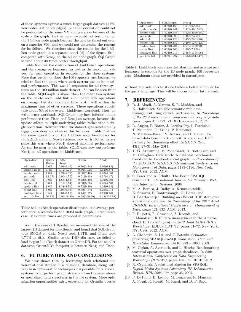
of these systems against a much larger graph dataset (1 bil-lion nodes, 4.3 billion edges), but that evaluation could notbe performed on the same VM configuration because of thescale of the graph. Furthermore, we could not test Titan onthe 1 billion node graph because the queries timed out evenon a superior VM, and we could not determine the reasonsfor its failure. We therefore show the results for the 1 bil-lion node graph in a separate panel (d) of the figure. Still,compared with Neo4j, on the billion node graph, SQLGraphshowed about 30 times better throughput.

Table 6 shows the distribution of LinkBench operations,and the average performance (as well as the maximum val-ues) for each operation in seconds for the three systems.Note that we do not show the 100 requester case because wetried to find the point where each system was at its maxi-mal performance. This was 10 requesters for all three sys-tems on the 100 million node dataset. As can be seen fromthe table, SQLGraph is slower than the other two systemson the delete node, add link and update link operationson average, but its maximum time is still well within themaximum time of other systems. These operations consti-tute about 5% of the overall LinkBench workload. Thus, onwrite-heavy workloads, SQLGraph may have inferior updateperformance than Titan and Neo4j on average, because theupdate affects multiple underlying tables rather than a sin-gle operation. However when the dataset gets substantiallybigger, one does not observe this behavior. Table 7 showsthe same operations on the 1 billion node benchmark forthe SQLGraph and Neo4j systems, now with 100 requesterssince this was where Neo4j showed maximal performance.As can be seen in the table, SQLGraph now outperformsNeo4j on all operations on LinkBench.

Operation Query SQL- Titan Neo4jDisbn Graph

add node 2.6% 0.04(0.47) 0.30(3.34) 0.96(6.13)update node 7.4% 0.12(1.75) 0.56(10.25) 1.12(6.87)delete node 1.0% 2.24(5.81) 0.98(7.45) 0.73(4.06)get node 12.9% 0.06(1.75) 0.51(9.18) 0.17(4.47)add link 9.0% 1.68(4.83) 0.72(6.40) 1.02(6.30)delete link 3.0% 0.12(1.54) 0.63(5.95) 0.28(4.50)update link 8.0% 1.38(4.70) 0.72(9.29) 1.02(6.33)count link 4.9% 0.03(0.53) 0.52(7.54) 0.22(5.31)multiget link 0.5% 0.04(0.15) 0.44(1.27) 0.19(0.48)get link list 50.7% 0.03(18.80) 0.58(369.30) 0.28(255.19)

Table 6: LinkBench operation distribution, and average per-formance in seconds for the 100M node graph, 10 requesterscase. Maximum times are provided in parentheses.

As in the case of DBpedia, we measured the size of thelargest 1B dataset for LinkBench, and found that SQLGraphtook 850GB on disk, Neo4j took 1.1TB, and Titan took1.7TB on disk. Similar to the DBPedia case, we failed toload largest LinkBench dataset to OrientDB. For the smallerdatasets, OrientDB’s footprint is between Neo4j and Titan.

6. FUTURE WORK AND CONCLUSIONSWe have shown that by leveraging both relational and

non-relational storage in a relational database, along withvery basic optimization techniques it is possible for relationalsystems to outperform graph stores built on key value storesor specialized data structures in the file system. More opti-mization opportunities exist, especially for Gremlin queries

Operation SQLGraph Neo4jadd node 0.002(0.160) 1.643(6.586)update node 0.003(0.241) 2.429(490.562)delete node 0.422(0.586) 4.527(2059.552)get node 0.002(0.093) 1.453(7.259)add link 0.405(0.723) 2.435(786.816)delete link 0.003(0.152) 2.297(1273.229)update link 0.307(0.704) 2.677(1132.209)count link 0.002(0.266) 1.505(7.128)multiget link 0.004(0.013) 2.387(1165.061)get link list 0.002(1.297) 1.651(684.347)

Table 7: LinkBench operation distribution, and average per-formance in seconds for the 1B node graph, 100 requesterscase. Maximum times are provided in parentheses.

without any side effects, if one builds a better compiler forthe query language. This will be a focus for our future work.

7. REFERENCES[1] D. J. Abadi, A. Marcus, S. R. Madden, and

K. Hollenbach. Scalable semantic web datamanagement using vertical partitioning. In Proceedingsof the 33rd international conference on very large databases, pages 411–422. VLDB Endowment, 2007.

[2] R. Angles, P. Boncz, J. Larriba-Pey, I. Fundulaki,T. Neumann, O. Erling, P. Neubauer,N. Martinez-Bazan, V. Kotsev, and I. Toma. Thelinked data benchmark council: A graph and RDFindustry benchmarking effort. SIGMOD Rec.,43(1):27–31, May 2014.

[3] T. G. Armstrong, V. Ponnekanti, D. Borthakur, andM. Callaghan. LinkBench: A database benchmarkbased on the Facebook social graph. In Proceedings ofthe 2013 ACM SIGMOD International Conference onManagement of Data, pages 1185–1196, New York,NY, USA, 2013. ACM.

[4] C. Bizer and A. Schultz. The Berlin SPARQLbenchmark. International Journal On Semantic Weband Information Systems, 2009.

[5] M. A. Bornea, J. Dolby, A. Kementsietsidis,K. Srinivas, P. Dantressangle, O. Udrea, andB. Bhattacharjee. Building an efficient RDF store overa relational database. In Proceedings of the 2013 ACMSIGMOD International Conference on Management ofData, pages 121–132. ACM, 2013.

[6] F. Bugiotti, F. Goasdoue, Z. Kaoudi, andI. Manolescu. RDF data management in the Amazoncloud. In Proceedings of the 2012 Joint EDBT/ICDTWorkshops, EDBT-ICDT ’12, pages 61–72, New York,NY, USA, 2012. ACM.

[7] A. Chebotko, S. Lu, and F. Fotouhi. Semanticspreserving SPARQL-to-SQL translation. Data andKnowledge Engineering, 68(10):973 – 1000, 2009.

[8] M. Ciglan, A. Averbuch, and L. Hluchy. Benchmarkingtraversal operations over graph databases. In 28thInternational Conference on Data EngineeringWorkshops (ICDEW), pages 186–189. IEEE, 2012.

[9] R. Cyganiak. A relational algebra for SPARQL.Digital Media Systems Laboratory HP LaboratoriesBristol. HPL-2005-170, page 35, 2005.

[10] F. Di Pinto, D. Lembo, M. Lenzerini, R. Mancini,A. Poggi, R. Rosati, M. Ruzzi, and D. F. Savo.

Optimizing query rewriting in ontology-based dataaccess. In Proceedings of the 16th InternationalConference on Extending Database Technology, EDBT’13, pages 561–572, New York, NY, USA, 2013. ACM.

[11] D. Dominguez-Sal, P. Urbon-Bayes, A. Gimenez-Vano,S. Gomez-Villamor, N. Martınez-Bazan, and J.-L.Larriba-Pey. Survey of graph database performance onthe HPC scalable graph analysis benchmark. InWeb-Age Information Management, pages 37–48.Springer, 2010.

[12] Y. Guo, Z. Pan, and J. Heflin. LUBM: A benchmarkfor OWL knowledge base systems. Journal of WebSemantics, 3(2–3):158–182, 2005.

[13] S. Harris and N. Shadbolt. SPARQL query processingwith conventional relational database systems. In WebInformation Systems Engineering–WISE 2005Workshops, pages 235–244. Springer, 2005.

[14] O. Hartig and B. Thompson. Foundations of analternative approach to reification in RDF. CoRR,abs/1406.3399, 2014.

[15] F. Holzschuher and R. Peinl. Performance of graphquery languages: Comparison of Cypher, Gremlin andnative access in Neo4J. In Proceedings of the JointEDBT/ICDT 2013 Workshops, pages 195–204, NewYork, NY, USA, 2013. ACM.

[16] J. Huang, D. J. Abadi, and K. Ren. Scalable SPARQLquerying of large RDF graphs. PVLDB,4(11):1123–1134, 2011.

[17] S. Jouili and V. Vansteenberghe. An empiricalcomparison of graph databases. In SocialCom, pages708–715. IEEE, 2013.

[18] Z. Kaoudi and I. Manolescu. Cloud-based RDF datamanagement. In Proceedings of the 2014 ACMSIGMOD International Conference on Management ofData, pages 725–729, New York, NY, USA, 2014.ACM.

[19] L. Ma, Y. Yang, Z. Qiu, G. Xie, Y. Pan, and S. Liu.Towards a complete OWL ontology benchmark. InProceedings of the 3rd European Conference on TheSemantic Web, ESWC’06, pages 125–139, Berlin,Heidelberg, 2006. Springer-Verlag.

[20] P. Macko, D. Margo, and M. Seltzer. Performanceintrospection of graph databases. In Proceedings of the6th International Systems and Storage Conference,page 18. ACM, 2013.

[21] N. Martınez-Bazan, V. Muntes-Mulero,S. Gomez-Villamor, J. Nin, M.-A. Sanchez-Martınez,and J.-L. Larriba-Pey. DEX: High-performanceexploration on large graphs for information retrieval.In Proceedings of the Sixteenth ACM Conference onConference on Information and KnowledgeManagement, CIKM ’07, pages 573–582, New York,NY, USA, 2007. ACM.

[22] M. Morsey, J. Lehmann, S. Auer, and A.-C. N.Ngomo. DBpedia SPARQL benchmark–performanceassessment with real queries on real data. In TheSemantic Web–ISWC 2011, pages 454–469. Springer,2011.

[23] R. C. Murphy, K. B. Wheeler, B. W. Barrett, andJ. A. Ang. Introducing the graph 500. Cray UsersGroup (CUG), 2010.

[24] T. Neumann and G. Weikum. RDF-3X: A RISC-styleengine for RDF. Proc. VLDB Endow., 1(1):647–659,Aug. 2008.

[25] T. Neumann and G. Weikum. x-RDF-3X: Fastquerying, high update rates, and consistency for RDFdatabases. Proc. VLDB Endow., 3(1-2):256–263, Sept.2010.

[26] K. Nitta and I. Savnik. Survey of RDF storagemanagers. In DBKDA 2014, The Sixth InternationalConference on Advances in Databases, Knowledge,and Data Applications, pages 148–153, 2014.

[27] N. Papailiou, I. Konstantinou, D. Tsoumakos, andN. Koziris. H2RDF: Adaptive query processing onRDF data in the cloud. In Proceedings of the 21stInternational Conference Companion on World WideWeb, WWW ’12 Companion, pages 397–400, NewYork, NY, USA, 2012. ACM.

[28] N. Papailiou, D. Tsoumakos, I. Konstantinou,P. Karras, and N. Koziris. H2RDF+: an efficient datamanagement system for big RDF graphs. InProceedings of the ACM SIGMOD InternationalConference on Management of Data, SIGMOD 2014,Snowbird, Utah, USA on June 22-27, 2014. ACM,2014.

[29] M. Rodrıguez-Muro, R. Kontchakov, andM. Zakharyaschev. Ontology-based data access:Ontop of databases. In International Semantic WebConference, ISWC 2013, pages 558–573. Springer,2013.

[30] S. S. Sahoo, W. Halb, S. Hellmann, K. Idehen,S. Auer, J. Sequeda, and A. Ezzat. A survey of currentapproaches for mapping of relational databases toRDF. W3C RDB2RDF XG Incubator Report, 2009.

[31] S. Sakr and G. Al-Naymat. Relational processing ofRDF queries: a survey. ACM SIGMOD Record,38(4):23–28, 2010.

[32] M. Schmidt, T. Hornung, G. Lausen, and C. Pinkel.SP2Bench: a SPARQL performance benchmark. InData Engineering, 2009. ICDE’09. IEEE 25thInternational Conference on, pages 222–233. IEEE,2009.

[33] M. Schmidt, M. Meier, and G. Lausen. Foundations ofSPARQL query optimization. In Proceedings of the13th International Conference on Database Theory,ICDT ’10, pages 4–33, New York, NY, USA, 2010.ACM.

[34] M. Stocker, A. Seaborne, A. Bernstein, C. Kiefer, andD. Reynolds. SPARQL basic graph patternoptimization using selectivity estimation. InProceedings of the 17th International Conference onWorld Wide Web, WWW ’08, pages 595–604, NewYork, NY, USA, 2008. ACM.

[35] Tinkerpop. Blueprints. Available:https://github.com/tinkerpop/blueprints/wiki, 2014.

[36] Tinkerpop. Gremlin pipes. Available:https://github.com/tinkerpop/pipes/wiki, 2014.

[37] Tinkerpop. Gremlin query language. Available:https://github.com/tinkerpop/gremlin/wiki, 2014.

[38] K. Wilkinson, C. Sayers, H. A. Kuno, andD. Reynolds. Efficient RDF Storage and Retrieval inJena2. In Semantic Web and Databases Workshop,pages 131–150, 2003.

[39] P. Yuan, P. Liu, B. Wu, H. Jin, W. Zhang, and L. Liu.Triplebit: A fast and compact system for large scaleRDF data. Proc. VLDB Endow., 6(7):517–528, May2013.

APPENDIXA. GREMLIN TRANSLATION IN DETAIL

As described in section 4.3, Gremlin queries can be trans-lated into SQL queries (CTEs) or stored procedure calls(SPs) based on a set of pre-defined templates. Table 8 givesa full list of Gremlin pipes that are currently supported byour query translator and the corresponding CTE templates.Here we only include the templates for the basic form ofthe pipes. Possible variations and combinations of the pipetranslation have been discussed in section 4.

B. SPARQL TO GREMLIN QUERY CON-VERSION

As described in section 5.1, our first DBPedia Gremlinquery set was converted from the SPARQL queries usedin [22]. Given the declarative nature of the SPARQL queries,we tried to implement each of the SPARQL query usinggraph traversals in Gremlin as efficient as possible. Morespecifically, we first identify the most selective URI as theGremlin start pipe, and then use Gremlin transform pipesto implement the SPARQL triple patterns. Note that thetraversal order of the transform pipes is also based on the se-lectivity of the different triple patterns. SPARQL filters aredirectly translated into Gremlin filter pipes, and SPARQLUNION operations are translated into Gremlin branch pipesif possible. In addition, the translated Gremlin queries willonly return the size of the result set of the correspond-ing SPARQL queries, to minimize the result set composingand consumption differences of the different property graphstores.

Table 9 gives an example of SPARQL query to Gremlinquery translation (dq2 in section 5.1). It can be seen thatthe URI ’http://dbpedia.org/ontology/Person’ is used in thestart pipe to lookup the start vertex. Then the property fil-ter pipe applies on the most selective literal ”Montreal Cara-bins”@en. The out pipe and back pipe are used to traversethe graph. Two table pipes are used to store the results ofthe main branch and the optional branch. Ideally, the outerleft join of the two tables generates the desired results of theoriginal SPARQL query. However, due to the lack of built-in table operation support in Gremlin language, we directlyreturn the sizes of the both tables in the translated Gremlinquery.

Lan-guage

Query

SPARQL PREFIX rdfs:<http://www.w3.org/2000/01/rdf-schema#>PREFIX dbpedia-owl: <http://dbpedia.org/ontology/>PREFIX foaf: <http://xmlns.com/foaf/0.1/>PREFIX dbpedia-prop: <http://dbpedia.org/property/>PREFIX rdf:<http://www.w3.org/1999/02/22-rdf-syntax-ns#>SELECT ?var4 ?var8 ?var10WHERE {

?var5 dbpedia-owl:thumbnail ?var4 ;rdf:type dbpedia-owl:Person ;rdfs:label ”Montreal Carabins”@en ;dbpedia-prop:pageurl ?var8 .OPTIONAL { ?var5 foaf:homepage ?var10 . }

}Gremlin t1=new Table();

t2=new Table();var5=[];g.V(” URI ”, ”http://dbpedia.org/ontology/Person”).in(’http://www.w3.org/1999/02/22-rdf-syntax-ns#type’).has(’http://www.w3.org/2000/01/rdf-schema#label’,’”Montreal Carabins”@en’).aggregate(var5).as(’var5’).out(’http://dbpedia.org/ontology/thumbnail’).as(’var4’).back(1).out(’http://dbpedia.org/property/pageurl’).as(’var8’).table(t1).iterate();var5. ().as(’var5’).out(’http://xmlns.com/foaf/0.1/homepage’).as(’var10’).table(t2).iterate();[t1.size(),t2.size()];

Table 9: An example of SPARQL to Gremlin query conver-sion.

Opera-tion

CTE Template for Query Translation

out pipe (t0, SELECT t.val FROM tin v,OPA p, TABLES(VALUES(p.val0), ... ,(p.valn))AS t(val) WHERE v.val=p.vid AND t.val isnot null), (t1,SELECT COALESCE(s.val, p.val) AS val FROM t0 p LEFT OUTER JOIN OSA s on p.val=s.valid)

in pipe (t0, SELECT t.val FROM tin v,IPA p, TABLES(VALUES(p.val0), ... ,(p.valm))AS t(val) WHERE v.val=p.vid AND t.val isnot null), (t1,SELECT COALESCE(s.val, p.val) AS val FROM t0 p LEFT OUTER JOIN ISA s on p.val=s.valid)

both pipe (t0, SELECT t.val FROM tin v,OPA p, TABLES(VALUES(p.val0), ... ,(p.valn))AS t(val) WHERE v.val=p.vid AND t.val isnot null), (t1, SELECT COALESCE(s.val, p.val) AS val FROM t0 p LEFT OUTER JOIN OSA s on p.val=s.valid), (t2,SELECT t.val FROM tin v,IPA p, TABLES(VALUES(p.val0), ... ,(p.valm))AS t(val) WHERE v.val=p.vid AND t.val is notnull), (t3,SELECT COALESCE(s.val, p.val) AS val FROM t2 p LEFT OUTER JOIN ISA s on p.val=s.valid), (t4,SELECT *FROM t1 UNION ALL SELECT * FROM t3)

outvertexpipe

(t0, SELECT p.outv AS val FROM tin v, EA p WHERE v.val=p.eid )

in vertexpipe

(t0, SELECT p.inv AS val FROM tin v, EA p WHERE v.val=p.eid )

bothvertexpipe

(t0, SELECT t.val FROM tin v, EA p, TABLES(VALUES(p.outv), (p.inv)) AS t(val) WHERE v.val=p.eid )

out edgespipe

(t0, SELECT p.eid AS val FROM tin v, EA p WHERE v.val=p.outv )

in edgespipe

(t0, SELECT p.eid AS val FROM tin v, EA p WHERE v.val=p.inv )

bothedgespipe

(t0, SELECT p.eid AS val FROM tin v, EA p WHERE v.val=p.outv OR v.val=p.inv )

rangefilterpipe

(t0, SELECT * FROM tin v LIMIT ? OFFSET ?)

duplicatefilterpipe

(t0, SELECT DISTINCT v.val FROM tin v)

id filterpipe

(t0, SELECT * FROM tin v WHERE v.val == ?)

propertyfilterpipe

(t0, SELECT v.* FROM tin v, VA p WHERE v.val=p.vid AND JSON VAL(p.data, ?) == ?)

intervalfilterpipe

(t0, SELECT v.* FROM tin v, VA p WHERE v.val=p.vid AND JSON VAL(p.data, ?) > ? AND JSON VAL(p.data, ?) < ?)

labelfilterpipe

(t0, SELECT v.* FROM tin v, EA p WHERE v.val=p.eid AND p.lbl == ?)

exceptfilterpipe

(t0, SELECT * FROM tin v WHERE v.val NOT IN (SELECT p.val FROM tk p) )

retainfilterpipe

(t0, SELECT * FROM tin v WHERE v.val IN (SELECT p.val FROM tk p) )

cyclicpathfilterpipe

(t0, SELECT * FROM tin v WHERE isSimplePath(v.path) == 1)

backfilterpipe

meta.cte ∪ (t0, SELECT * FROM tin v WHERE v.val IN (SELECT p.path[0] FROM meta.tout p))

and filterpipe

meta1.cte ∪ meta2.cte ∪ (t0, SELECT * FROM tin v WHERE v.val IN (SELECT p.path[0] FROM meta1.tout p1INTERSECT SELECT p.path[0] FROM meta2.tout p2))

or filterpipe

meta1.cte ∪ meta2.cte ∪ (t0, SELECT * FROM tin v WHERE v.val IN (SELECT p.path[0] FROM meta1.tout p1 UNIONSELECT p.path[0] FROM meta2.tout p2))

if-then-elsepipe

test.cte ∪ {thenctein, elsectein} ∪ then.cte ∪ else.cte ∪ (tout, SELECT * FROM then.out UNION ALL SELECT * FROMelse.out)

split-mergepipe

meta1.cte ∪ meta2.cte ∪ (t0, SELECT * FROM meta1.tout p1 UNION ALL SELECT * FROM meta2.tout p2)

loop pipe expand to fixed-length ctes or call stored procedureas pipe ∅, record the mapping between the as pipe and the (tout) of the current translated ctesaggregatepipe

∅, record the mapping between the aggregate pipe and the (tout) of the current translated ctes

addvertex

∅, call stored procedure

add edge ∅, call stored proceduredeletevertex

∅, call stored procedure

deleteedge

∅, call stored procedure

Table 8: Currently supported Gremlin pipes and the translation method. “?” denotes the parameters of the pipes.