Syracuse University Syracuse University

SURFACE SURFACE

Syracuse University Honors Program Capstone Projects

Syracuse University Honors Program Capstone Projects

Spring 5-2016

Models for Storing Relationships: Relational vs. Graph Databases Models for Storing Relationships: Relational vs. Graph Databases

Dylan Hantula

Follow this and additional works at: https://surface.syr.edu/honors_capstone

Part of the Management Information Systems Commons

Recommended Citation Recommended Citation Hantula, Dylan, "Models for Storing Relationships: Relational vs. Graph Databases" (2016). Syracuse University Honors Program Capstone Projects. 943. https://surface.syr.edu/honors_capstone/943

This Honors Capstone Project is brought to you for free and open access by the Syracuse University Honors Program Capstone Projects at SURFACE. It has been accepted for inclusion in Syracuse University Honors Program Capstone Projects by an authorized administrator of SURFACE. For more information, please contact surface@syr.edu.

Models for Storing Relationships: Relational vs. Graph Databases

A Capstone Project Submitted in Partial Fulfillment of the Requirements of the Renée Crown University Honors Program at

Syracuse University

Dylan Hantula Candidate for Bachelor of Science

Systems & Information Science and Renée Crown University Honors

May 2016

Honors Capstone Project in the School of Information Studies

Capstone Project Advisor: ____________________________________ Deborah Nosky

Capstone Project Reader: ____________________________________ Mark Costa

Honors Director: ____________________________________ Stephen Kuusisto, Director

Date: May 10, 2016

© Dylan Hantula 2016

iii

Abstract

Relational databases have been the universal industry standard for almost as long as

databases have existed. While relational databases are undoubtedly useful for storing

tabular data that fits into a pre-defined schema of rows and columns, they are not very

accommodating of interconnections within a data set. Forcing a highly connected data set

into a relational database commonly results in severe performance issues in query return

time. With the recent rise of social networks and other modern technological

advancements, data is quickly becoming more connected and thus less suitable for

relational databases. As a result, a new type of database, called a graph database, has

emerged to store relationship-oriented data naturally and efficiently using nodes and

edges. Deciding which database is more suitable for the task at hand is not always trivial,

however. This paper sheds light on the differences between the two databases and delves

into why one database might be more advantageous in certain situations.

iv

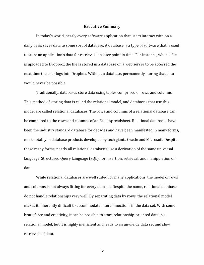
Executive Summary

In today’s world, nearly every software application that users interact with on a

daily basis saves data to some sort of database. A database is a type of software that is used

to store an application’s data for retrieval at a later point in time. For instance, when a file

is uploaded to Dropbox, the file is stored in a database on a web server to be accessed the

next time the user logs into Dropbox. Without a database, permanently storing that data

would never be possible.

Traditionally, databases store data using tables comprised of rows and columns.

This method of storing data is called the relational model, and databases that use this

model are called relational databases. The rows and columns of a relational database can

be compared to the rows and columns of an Excel spreadsheet. Relational databases have

been the industry standard database for decades and have been manifested in many forms,

most notably in database products developed by tech giants Oracle and Microsoft. Despite

these many forms, nearly all relational databases use a derivation of the same universal

language, Structured Query Language (SQL), for insertion, retrieval, and manipulation of

data.

While relational databases are well suited for many applications, the model of rows

and columns is not always fitting for every data set. Despite the name, relational databases

do not handle relationships very well. By separating data by rows, the relational model

makes it inherently difficult to accommodate interconnections in the data set. With some

brute force and creativity, it can be possible to store relationship-oriented data in a

relational model, but it is highly inefficient and leads to an unwieldy data set and slow

retrievals of data.

v

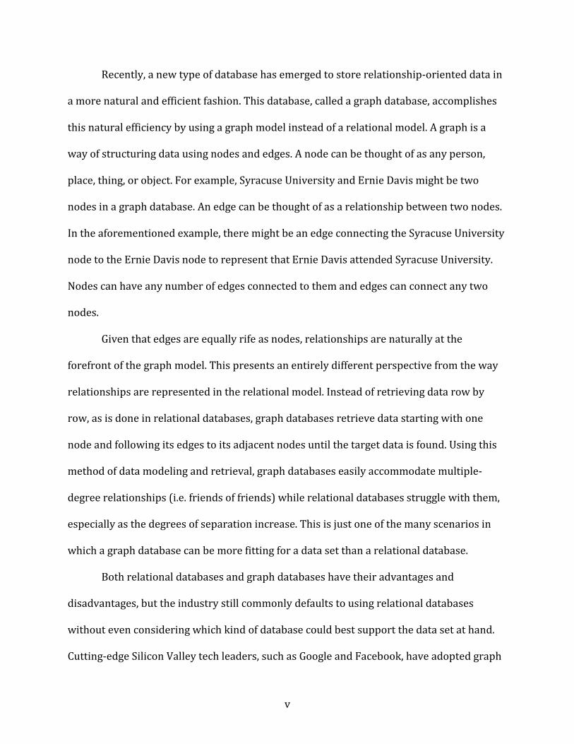
Recently, a new type of database has emerged to store relationship-oriented data in

a more natural and efficient fashion. This database, called a graph database, accomplishes

this natural efficiency by using a graph model instead of a relational model. A graph is a

way of structuring data using nodes and edges. A node can be thought of as any person,

place, thing, or object. For example, Syracuse University and Ernie Davis might be two

nodes in a graph database. An edge can be thought of as a relationship between two nodes.

In the aforementioned example, there might be an edge connecting the Syracuse University

node to the Ernie Davis node to represent that Ernie Davis attended Syracuse University.

Nodes can have any number of edges connected to them and edges can connect any two

nodes.

Given that edges are equally rife as nodes, relationships are naturally at the

forefront of the graph model. This presents an entirely different perspective from the way

relationships are represented in the relational model. Instead of retrieving data row by

row, as is done in relational databases, graph databases retrieve data starting with one

node and following its edges to its adjacent nodes until the target data is found. Using this

method of data modeling and retrieval, graph databases easily accommodate multiple-

degree relationships (i.e. friends of friends) while relational databases struggle with them,

especially as the degrees of separation increase. This is just one of the many scenarios in

which a graph database can be more fitting for a data set than a relational database.

Both relational databases and graph databases have their advantages and

disadvantages, but the industry still commonly defaults to using relational databases

without even considering which kind of database could best support the data set at hand.

Cutting-edge Silicon Valley tech leaders, such as Google and Facebook, have adopted graph

vi

databases for some of their applications, but a substantial portion of the tech industry

remains unaware that there could be a better option than a relational database. This

project goes beyond a simple comparison of two databases to examine a new technology

against an elder one, raise awareness about a future big player in the database world, and

open a debate about why one database might be more advantageous than another in some

situations.

vii

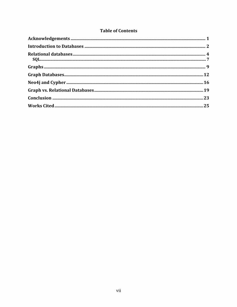
Table of Contents

Acknowledgements .............................................................................................................................. 1

Introduction to Databases ................................................................................................................. 2

Relational databases ............................................................................................................................ 4 SQL.......................................................................................................................................................................... 7

Graphs ....................................................................................................................................................... 9

Graph Databases .................................................................................................................................. 12

Neo4j and Cypher ................................................................................................................................ 16

Graph vs. Relational Databases ...................................................................................................... 19

Conclusion ............................................................................................................................................. 23

Works Cited ........................................................................................................................................... 25

1

Acknowledgements

First and foremost, I would like to thank my parents for supporting my education at

Syracuse University. I would also like to thank Professor Deborah Nosky for her wise

advice as my Honors Capstone Advisor and Mark Costa for taking time out of his busy

schedule as a PhD candidate to be my Honors Reader. Lastly, I would like to thank Dr. Jian

Qin for first introducing me to graph database research when I worked on her GenBank

Research Project.

2

Chapter 1

Introduction to Databases

A database is a collection of stored information organized in such a way that a

computer program can quickly retrieve desired pieces of data. Theoretically, a database

could exist in any number of mediums or formats, but in this case, databases are digital and

exist as software on computers. Some people describe databases as, “the basic electronic

information storage unit.” The main attributes of a database are the ability to add

information to the database, often called “inserting,” and the ability to read information

that has been previously added to the database. The act of calling for information that is

stored in a database is often called “querying” the database.

Databases can be seen in many aspects of the average American’s daily life. A

famous example of a database is the catalogue of books at a library. The catalogue stores

the title, author, publication year, and other pertinent information about every book in the

library. When the library gets a new book, the book is added to the catalogue. Library

patrons and librarians can search, or query, the catalogue to find a specific book or a list of

books with some commonality.

Many times, people may interact with databases without even realizing it. Nearly

every website on the Internet – most notably, social media websites – interacts with a

database in some fashion. Facebook, Twitter, Instagram, and other popular services use

databases to store all of the information that users post. In other words, all of the pictures,

comments, friend connections, and other online interactions between users are stored in

3

databases. When a user logs onto a social media website to check what has been recently

posted, he or she is essentially querying a database.

Databases exist in many forms and are constantly evolving as time goes on.

Historically, the relational database was the standard database to use for almost

everything. Recently, however, a new breed of databases – called NoSQL databases – has

sprung up to meet the demands of modern applications. Several different databases models

fall under the NoSQL database umbrella, including graph databases, document databases,

key-value stores, and wide-column stores. While each of these database models have their

place in modern technology, this paper will focus on one of the most widely used NoSQL

databases models, the graph database, pitted against the long-time leader of the database

world, the relational database.

4

Chapter 2

Relational databases

Databases come in countless forms with many different ways of modeling the data

they contain. One of the most popular and widely used types of databases is called a

relational database. A relational database uses a structured data model to store

information tables that are composed of rows and columns. Although tables in relational

databases are more complex, their structure of rows and columns can be visualized as a

spreadsheet.

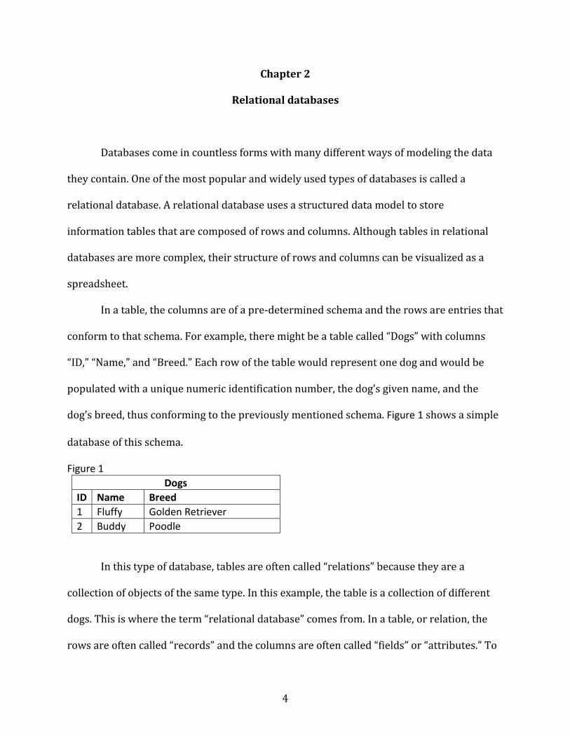
In a table, the columns are of a pre-determined schema and the rows are entries that

conform to that schema. For example, there might be a table called “Dogs” with columns

“ID,” “Name,” and “Breed.” Each row of the table would represent one dog and would be

populated with a unique numeric identification number, the dog’s given name, and the

dog’s breed, thus conforming to the previously mentioned schema. Figure 1 shows a simple

database of this schema.

Figure 1 Dogs

ID Name Breed 1 Fluffy Golden Retriever 2 Buddy Poodle

In this type of database, tables are often called “relations” because they are a

collection of objects of the same type. In this example, the table is a collection of different

dogs. This is where the term “relational database” comes from. In a table, or relation, the

rows are often called “records” and the columns are often called “fields” or “attributes.” To

5

differentiate one row from another, each row has a field called a primary key that uniquely

defines that row. In Figure 1, each row’s primary key is its ID field. This is because the ID is

guaranteed to be unique – there can not be any repeating values in this field. When using

primary keys, it is imperative that no two keys are the same so that each row can

successfully be differentiated. As such, using another field in Figure 1 as the primary key,

such as the name field, would be a poor choice because two dogs could potentially have the

same name. By using a different field that is guaranteed to be unique, such as numeric

identification numbers, users can differentiate between two dogs with the same name and

breed. The ability to refer to each row individually using unique primary keys is called

referential integrity and is the crux of the relational model. In some cases, a table can have

composite primary keys in which more than one field is grouped together to uniquely

define the rows. This will be explained in further detail later.

Although Figure 1 technically shows a relational database, it only has one table.

Essentially, the database in Figure 1 is no different than a common spreadsheet often found

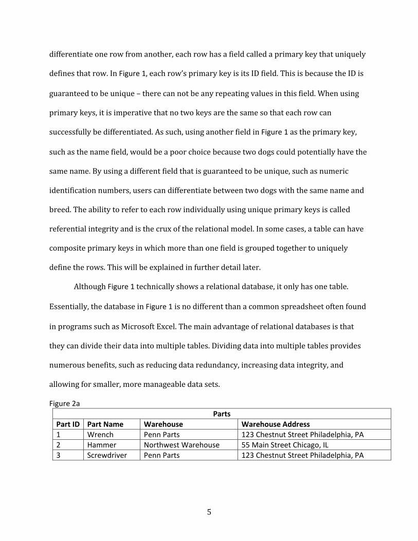
in programs such as Microsoft Excel. The main advantage of relational databases is that

they can divide their data into multiple tables. Dividing data into multiple tables provides

numerous benefits, such as reducing data redundancy, increasing data integrity, and

allowing for smaller, more manageable data sets.

Figure 2a Parts

Part ID Part Name Warehouse Warehouse Address 1 Wrench Penn Parts 123 Chestnut Street Philadelphia, PA 2 Hammer Northwest Warehouse 55 Main Street Chicago, IL 3 Screwdriver Penn Parts 123 Chestnut Street Philadelphia, PA

6

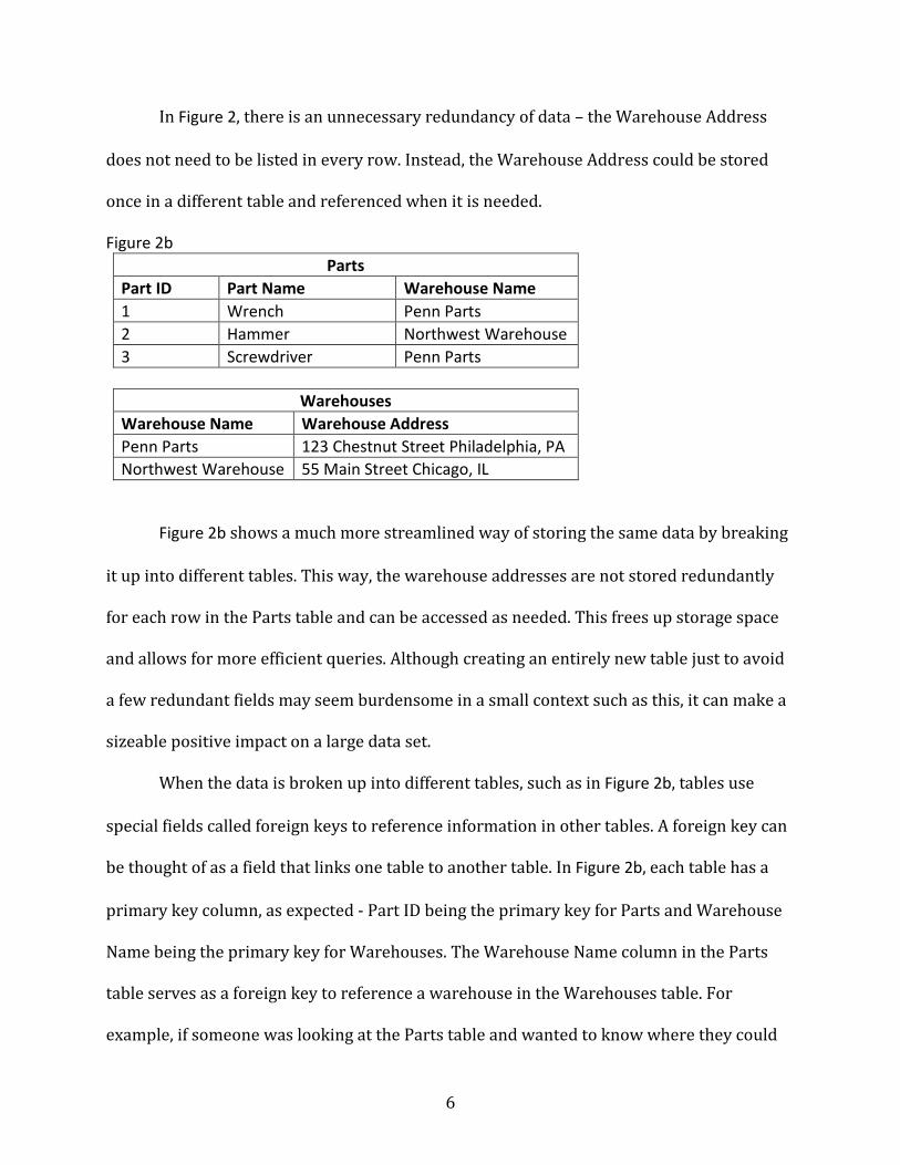
In Figure 2, there is an unnecessary redundancy of data – the Warehouse Address

does not need to be listed in every row. Instead, the Warehouse Address could be stored

once in a different table and referenced when it is needed.

Figure 2b Parts

Part ID Part Name Warehouse Name 1 Wrench Penn Parts 2 Hammer Northwest Warehouse 3 Screwdriver Penn Parts

Warehouses

Warehouse Name Warehouse Address Penn Parts 123 Chestnut Street Philadelphia, PA Northwest Warehouse 55 Main Street Chicago, IL

Figure 2b shows a much more streamlined way of storing the same data by breaking

it up into different tables. This way, the warehouse addresses are not stored redundantly

for each row in the Parts table and can be accessed as needed. This frees up storage space

and allows for more efficient queries. Although creating an entirely new table just to avoid

a few redundant fields may seem burdensome in a small context such as this, it can make a

sizeable positive impact on a large data set.

When the data is broken up into different tables, such as in Figure 2b, tables use

special fields called foreign keys to reference information in other tables. A foreign key can

be thought of as a field that links one table to another table. In Figure 2b, each table has a

primary key column, as expected - Part ID being the primary key for Parts and Warehouse

Name being the primary key for Warehouses. The Warehouse Name column in the Parts

table serves as a foreign key to reference a warehouse in the Warehouses table. For

example, if someone was looking at the Parts table and wanted to know where they could

7

find a screwdriver, he or she could see that screwdrivers are at Penn Parts. To find out

specifically where the Penn Parts warehouse is located, he or she could take the warehouse

name from the Parts table and “cross-reference” it with the Warehouses table to get the

address of that warehouse. This notion of taking data from one table and “cross-

referencing” with another table to get more information is called joining the tables.

SQL

Humans interact with databases using querying languages that have commands for

selecting, inserting, and deleting information, as well as other basic functions that are

necessary for a database. Relational databases commonly use a language called Structured

Query Language, or “SQL” for short. One of the main principles of SQL is that it allows the

user to focus on what data should be selected, rather than how to select it. In other words,

the user writes a SQL statement to ask the database for specific data, but the database

“decides” for itself how to find that information when executing the user’s SQL statement.

This can be likened to a simple Google search: the user types a search into Google and

receives the search results, but the user does not specify how the Google search engine

should approach it’s finding of the results.

SQL commands are commonly broken up into two main categories: Data

Manipulation Language (DML) and Data Definition Language (DDL). DML commands

handle interactions with the data itself, such as selecting, inserting, and deleting. In the

previously mentioned Google search example, the user’s search can be likened to a select

command in SQL. DDL commands handle interactions with the database, such as creating

8

or deleting tables and other database entities. DML and DDL commands are equally

necessary and integral to successfully using a relational database, or any database for that

matter. Although SQL, DML, and DDL are unique to relational databases, databases of all

kinds require some sort of system that allows users to interact with both the data and the

database itself.

9

Chapter 3

Graphs

Graph theory was pioneered by Euler in the 18th century and is known to be

applicable in a variety of mathematical problems. In its most simple form, a graph is

nothing more than a collection of nodes and the relationships among the nodes. A node can

be thought of as any kind of entity – any person, place, thing, or object. Graphs often include

several nodes, and these nodes are connected to one another by relationships called edges.

Edges connect two and only two nodes; edges cannot leave one node without terminating

at another node. Figure 3 shows a rudimentary graph that connects friends to one another.

In this example, the nodes represent people and the edges between them represent

friendships.

Figure 3

Nodes can be connected to zero, one, or many other nodes. In Figure 3, each node is

connected to either two or three other nodes. Not every node is interconnected, however.

For example, Ben is friends with David and Rob, and Rob is friends with Ben and Bobby, but

10

Ben is not friends with Bobby. Although Ben and Bobby cannot be considered friends in

this scenario without a direct edge, a connection can be made between Ben and Bobby by

following connections through either Rob or David. Connecting two otherwise unconnected

nodes by going through other nodes and edges is called traversing a graph. Traversing a

graph is one of the most basic graph operations and plays a major role in how graphs

execute queries. Queries are executed by traversing through the nodes of the graph to find

the data being queried. It is entirely possible to have an edge from each node to every

single other node in the entire graph. In such a scenario where the graph has many edges,

the graph is called a dense graph. On the other hand, a graph with few edges is called a

sparse graph. This distinction becomes important when deciding the most efficient way to

traverse through a given graph.

There are different types of graphs that have specific rules governing how the edges

are situated. In an undirected graph, edges go both ways. Figure 3 is an example of an

undirected graph (i.e. there is no difference is saying Ben is friends with Rob and Rob is

friends with Ben – the relationship goes both ways). A popular example of an undirected

relationship that people often encounter in everyday life is Facebook friendships. One

person sends a friend request to another person who then accepts the request. Once the

request is accepted, the two people are undirected friends.

In a directed graph, relationships only go one way (i.e. Person A is friends with

Person B, but Person B is not friends with Person A). A popular example of this that people

often encounter in everyday life is the notion of following someone on Twitter. One person

can follow another person on Twitter without that person following them back. Barack

Obama has 69.3 million followers on Twitter, but is only following 638,000 people. That

11

means that there are several million people who follow Barack Obama, but are not followed

by Barack Obama. This is an example of a directed relationship.

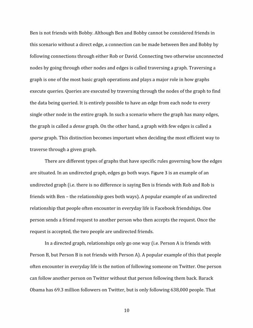
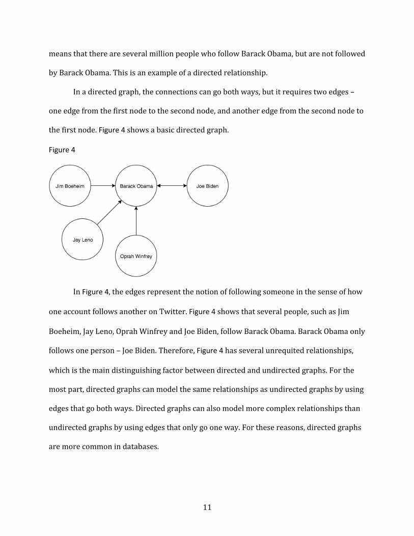
In a directed graph, the connections can go both ways, but it requires two edges –

one edge from the first node to the second node, and another edge from the second node to

the first node. Figure 4 shows a basic directed graph.

Figure 4

In Figure 4, the edges represent the notion of following someone in the sense of how

one account follows another on Twitter. Figure 4 shows that several people, such as Jim

Boeheim, Jay Leno, Oprah Winfrey and Joe Biden, follow Barack Obama. Barack Obama only

follows one person – Joe Biden. Therefore, Figure 4 has several unrequited relationships,

which is the main distinguishing factor between directed and undirected graphs. For the

most part, directed graphs can model the same relationships as undirected graphs by using

edges that go both ways. Directed graphs can also model more complex relationships than

undirected graphs by using edges that only go one way. For these reasons, directed graphs

are more common in databases.

12

Chapter 4

Graph Databases

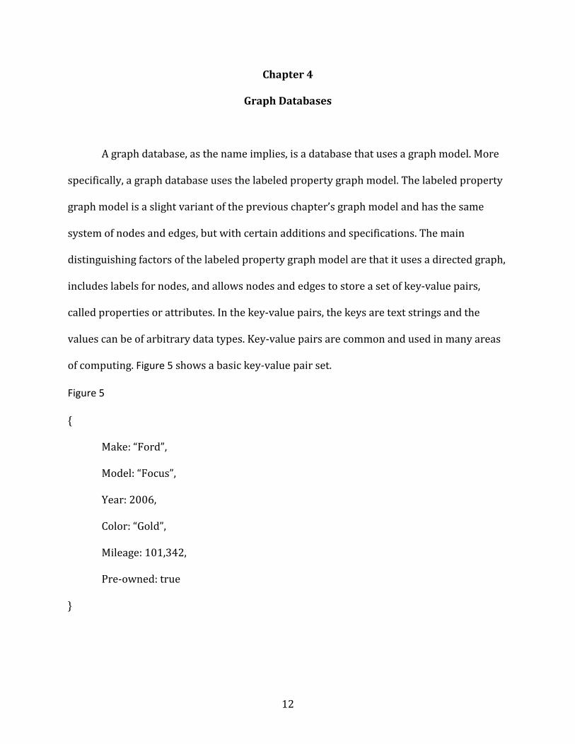
A graph database, as the name implies, is a database that uses a graph model. More

specifically, a graph database uses the labeled property graph model. The labeled property

graph model is a slight variant of the previous chapter’s graph model and has the same

system of nodes and edges, but with certain additions and specifications. The main

distinguishing factors of the labeled property graph model are that it uses a directed graph,

includes labels for nodes, and allows nodes and edges to store a set of key-value pairs,

called properties or attributes. In the key-value pairs, the keys are text strings and the

values can be of arbitrary data types. Key-value pairs are common and used in many areas

of computing. Figure 5 shows a basic key-value pair set.

Figure 5

{

Make: “Ford”,

Model: “Focus”,

Year: 2006,

Color: “Gold”,

Mileage: 101,342,

Pre-owned: true

}

13

The purpose of properties is to hold more information about the nodes and edges.

Labels are used as tags to group nodes of the same category together and to represent their

different roles in the data set. To simplify the labeled property graph model, some people

like to think of nodes as nouns that can be categorized by labels, edges as verbs, and

properties as adjectives. Figure 6a shows a graph using the labeled property graph model.

Both nodes and edges can have properties, but only nodes can have labels. Nodes and edges

can have zero or many attributes. Nodes can have zero or more labels.

Figure 6a

The labeled property graph’s inclusion of labels and attributes has a profound effect

on data modeling in the database. In a standard graph model, every data item must be

modeled as either a node or an edge. This makes data modeling easier because there are

14

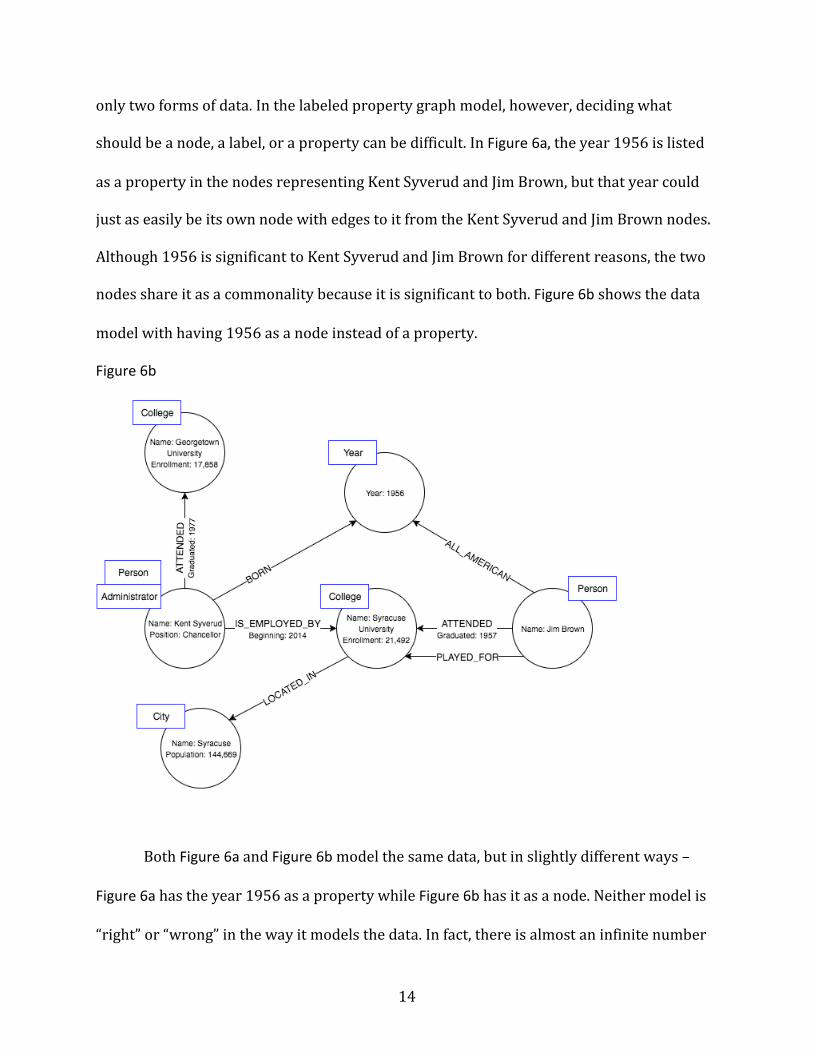
only two forms of data. In the labeled property graph model, however, deciding what

should be a node, a label, or a property can be difficult. In Figure 6a, the year 1956 is listed

as a property in the nodes representing Kent Syverud and Jim Brown, but that year could

just as easily be its own node with edges to it from the Kent Syverud and Jim Brown nodes.

Although 1956 is significant to Kent Syverud and Jim Brown for different reasons, the two

nodes share it as a commonality because it is significant to both. Figure 6b shows the data

model with having 1956 as a node instead of a property.

Figure 6b

Both Figure 6a and Figure 6b model the same data, but in slightly different ways –

Figure 6a has the year 1956 as a property while Figure 6b has it as a node. Neither model is

“right” or “wrong” in the way it models the data. In fact, there is almost an infinite number

15

of different ways to model this data by changing which data items are represented by

nodes, edges, properties, or labels. Certain models are more suited for certain use cases,

and deciding the most appropriate way to model the data for the given use case is an

important part of using a graph database, or a graph model in general.

Decisions about how to model data are dictated by how the data will be queried and

used. Labels should be used when data needs to be queried by category, such as compiling

a list of all of the colleges in the database. All nodes labeled with the same label belong to

the same set. Nodes are one of the fundamental units that form a graph and should be used

to represent entities, such as people, places, or things. Edges, the other fundamental unit

that forms a graph, should be used to represent interactions between entities – i.e.

someone attended a university. Properties give further detail about entities and

relationships and should be used to store information that is not already modeled by an

entity, relationship, or label.

16

Chapter 5

Neo4j and Cypher

Although relational databases and graph theory have both been around for decades,

commercially used graph databases are still relatively new. Several graph database

products have entered the market to serve the growing popularity of graph databases, but

many of the products have not fully matured yet. Some of the bigger tech companies create

their own in-house graph database solutions instead of using a commercially available

graph database product. Despite this, one commercially available graph database has stood

out above and beyond the rest: Neo4j.

In the year 2000, the founders of Neo Technology suffered so many performance

issues with relational databases that they decided it was time to look for a database that

used a graph model. Much to their dismay, they couldn’t find one. So, they decided to build

one. Neo Technology developed the first version of Neo4j in 2002. Neo4j has since become

the most popular and refined of the commercially available graph database products,

having been adopted by large corporations such as eBay and Walmart. All examples of

graph databases in the remainder of this report will be applicable to Neo4j

While relational databases have thrived for decades using SQL, graph databases

need a different querying language that lends itself well to the graph model. As such, Neo4j

has its own language that it uses called Cypher. Although SQL is nearly ubiquitous across

the many databases in the relational database world, the Cypher language was created by

Neo Technology and is specific to Neo4j. With the great success Neo Technology has found

with its Neo4j database, there has been a recent movement to spread Cypher to other

17

graph databases, similar to how SQL is used by nearly all relational databases. This

movement is led by the openCypher project and backed by Neo Technology with the goal of

making Cypher available to everyone. If the openCypher project is successful, Cypher will

be ubiquitous across nearly all graph databases and will be “the SQL of graph databases.”

At a high level, Cypher accomplishes the same basic tasks that SQL does in terms of

manipulating data and database objects as requested by the user’s query. In use, however,

Cypher is different than SQL in the way queries are written to select the data. Unlike SQL,

Cypher allows users to ask the database to return data that match a specific pattern.

Queries can be written to return all data that matches a given general pattern regardless of

what nodes are involved, or more specificity can be added to restrict the pattern to only

include connections involving certain nodes. For example, going back to Figure 6b, a user

could write a query to return all pairs of nodes in which one node “attended” another node

(i.e. Node A attended Node B). The result of this query for the graph in Figure 6b would

show that Jim Brown attended Syracuse University and Kent Syverud attended Georgetown

University. This query could be made more specific by only asking for the schools in which

a specific node, such as Kent Syverud, attended. In that case, the results of the query would

only show that Kent Syverud attended Georgetown University.

In addition to pattern queries, users can write “SQL-esque” queries that specify

exactly what data should be returned, such as getting a list of all nodes of a specific type.

Again using Figure 6b as an example, a user could write a query asking for all nodes of the

type “college” which would return Syracuse University and Georgetown University. This

kind of flexibility in the way that queries can be written is a huge advantage to Neo4j, and

graph databases as a whole. Through searching based on patterns and data types, the user

18

has a variety of options of how to select the desired data. By taking full advantage of these

query options and the inherent connected nature of the graph structure, the user can write

queries to return groups of data that relational databases would have great difficulty

connecting.

19

Chapter 6

Graph vs. Relational Databases

Relational databases were originally designed to codify paper forms and tabular

structures, and they do this quite well. They require a rigid pre-defined schema for the data

that can be unforgiving to changes and unexpected relationships that pop up unexpectedly.

Ironically, relational databases are not very accommodating of modeling

relationships. This is because they rely on foreign keys to relate one piece of information to

another, rather than explicitly storing relationships. This system of referencing keys in

other tables works for simple relationships, but poses serious performance problems once

the relationships become multi-faceted. The main source of this problem is the fact that

tables need to be “joined” together on their foreign keys in order to combine information

from different tables. Joins can be computationally expensive, so joining together several

different tables to query a relationship that spans several entities can take a long time.

Figure 7 People

ID Name 1 Nick 2 Matthew 3 Adam 4 Jaimie 5 Nolan

Connections Person_ID Connection_ID 1 2 1 3 2 3 2 5 3 1 3 2 4 3 4 5 5 4

20

In Figure 7, there is one table representing people and one table representing

relationships between those people. Each person in the People table is assigned a numeric

ID. In the Connections table, a person’s ID in the People table is referenced as either a

Person_ID or a Connection_ID; both the Person_ID and Connection_ID columns in the

Connections table refer to IDs in the People table. For example, Nick (ID 1) is connected to

Matthew (ID 2) and Adam (ID 3).

In the People table, the ID column is the primary key. On the other hand, the

Connections table uses a composite primary key of both the Person_ID and the

Connection_ID columns. A composite primary key requires both columns to be a unique

combination of values. For example, Person_ID = 1 and Connection_ID = 2 is a different

composite value than Person_ID = 1 and Connection_ID = 3. Depending on if directed

relationships need to be modeled, some relational database configurations store composite

values such as Person_ID = 1 and Connection_ID = 3 as being a completely different

composite than Person_ID = 3 and Connection_ID = 1. This is how unrequited relationships

can be modeled. For this example, however, the relationships are undirected, so it can be

assumed that Person_ID = 1 and Connection_ID = 3 is the same composite value as

Person_ID = 3 and Connection_ID = 1.

For simple queries, such as finding out who are Nick’s connections, the relational

model in Figure 7 works well. Essentially, the query looks at the People table, finds which ID

is associated with Nick, takes that ID to the Connections table, finds all the Connection_IDs

that are associated with Nick’s Person_ID, then references those Connection_IDs back to the

People table to find the names associated with those Connection_IDs. While this may seem

complicated, it is a streamlined process that most humans do subconsciously when looking

21

at spreadsheets. A similar process is used to answer the question, “Who is connected to

Nick?” Given that the connections are directed, the questions “Who is connected to Nick?”

and “Who is Nick connected to?” are actually two different queries with two different result

sets.

Issues begin to arise when more in-depth questions are asked, such as “Who are the

connections of Nick’s connections?” This requires doing all of the aforementioned work

that was done to find out who Nick’s connections are, and then iterating through each of

Nick’s connections to do the same process to find each of their connections. While this type

of query is still possible with the relational model of Figure 7, it is computationally

expensive. Taking it one step further, answering the question, “Who are the connections of

the connections of Nick’s connections?” is even more computationally expensive with a

relational model, to the point where it can be nearly impossible at times. This type of query

may be difficult to grasp when worded in such a way, but it is actually a scenario that

manifests itself in everyday life. LinkedIn’s system of connections is a famous example of

this. LinkedIn has first, second, and third connections. A first connection is someone who a

user is directly connected to. A second connection is a connection of a user’s first

connection. A third connection is a connection of a user’s second connection. Going back to

the previous example, finding Nick’s third connections on LinkedIn would require

answering the question, “Who are the connections of the connections of Nick’s

connections?”

While the LinkedIn model of connections may be ill-suited for a relational model, it

works well in a graph model. Unlike in relational databases, relationships are considered

“first-class” citizens in graph databases because they are explicitly stored. Queries are

22

executed by traversing through the graph one node at a time via edges between the nodes.

As such, relationships that span several entities, such as the LinkedIn model of connections,

are actually fairly easy using a graph because the nodes are all connected. This differs from

a relational model in which a query is required to connect the necessary information

together by joining the necessary tables. In a graph, the information is inherently

connected simply by the nature of the graph data structure.

23

Chapter 7

Conclusion

When a new technology rises in popularity, there is usually one group of people who

support the technology wholeheartedly and another group of people who are loyal to the

old technologies and do not want to adopt anything new. Both positions are

understandable – jumping on a new technology to garner its benefits as soon as possible

could be advantageous, but sticking with a technology that has been proven to work in case

the new technology becomes a short fad could also be advantageous. Like most new

technologies, graph databases have been the focal point of this debate since their inception.

Unsurprisingly, organizations that rely heavily on data in their databases are very cautious

about maintaining the integrity, security and reliability of that data. As such, many

organizations can be reluctant to make a huge change in their database from a relational

model to a graph model.

Despite this reluctance, graph databases have been experiencing a sharp increase in

adoption by small and large organizations alike who could benefit from the graph model.

Organizations that deal with heavily connected data and place importance on relationships

within data are starting to realize that the relational model will only cause more issues as

their data sets grow. Conversely, organizations that work with tabular data that requires a

rigid structure have long understood that the relational model suits them well and that

switching to a graph model would be detrimental.

We live in an exciting time period in the world of databases with the recent rise of

graph and other NoSQL databases. Graph databases are certainly not the best suited for all

24

applications, but they are finally getting the consideration they deserve by organizations

that could benefit from them. If the industry keeps progressing on this trajectory, the

relational model will not be the automatic default database in the industry. Rather,

organizations will finally start using the database that fits their needs the best.

25

Works Cited

"A Relational Database Overview." (The Java™ Tutorials JDBC(TM) Database Access JDBC Introduction). Oracle, n.d. Web. 07 Apr. 2016. <https://docs.oracle.com/javase/tutorial/jdbc/overview/database.html>.

Beal, Vangie. "What Is Database (DB)?" Webopedia. Webopedia, n.d. Web. 06 May 2016. Daly, Katharine M. "Hand-Drawn Graph Problems in Online Education." Massachusetts

Institute of Technology, June 2015. Web. 7 Apr. 2016. <https://dspace.mit.edu/bitstream/handle/1721.1/100303/930711715-MIT.pdf?sequence=1>.

Eifrem, Emil. "Meet OpenCypher: The SQL for Graphs - Neo4j Graph Database." Neo4j Blog. Neo Technology, 21 Oct. 2015. Web. 06 May 2016. <http://neo4j.com/blog/open-cypher-sql-for-graphs/>.

"Guide to Data Modeling." Neo4j Graph Database. Neo4j, n.d. Web. 07 Apr. 2016. <http://neo4j.com/developer/guide-data-modeling>.

"Neo4j - Labels vs Properties vs Relationship + Node." Stack Overflow. N.p., n.d. Web. 07 Apr. 2016. <http://stackoverflow.com/questions/22340475/neo4j-labels-vs-properties-vs-relationship-node>.

"NoSQL Databases Explained." MongoDB. MongoDB, n.d. Web. 06 May 2016. <https://www.mongodb.com/nosql-explained>.

"Primary and Foreign Keys." N.p., n.d. Web. 07 Apr. 2016. <http://condor.depaul.edu/gandrus/240IT/accesspages/primary-foreign-keys.htm>.

"Relational Database Concepts for Beginners." (n.d.): n. pag. 27 Mar. 2012. Web. 7 Apr. 2016. <http://webs.wofford.edu/whisnantdm/Courses/CS101/PDF/Database/Relational_database_concepts.pdf>.

"Relational Databases vs. Graph Databases: A Comparison." Neo4j Graph Database. Neo4j, n.d. Web. 07 Apr. 2016. <http://neo4j.com/developer/graph-db-vs-rdbms>.

"The Relational Model." N.p., 15 Feb. 2001. Web. 07 Apr. 2016. <http://www.siue.edu/~dbock/cmis450/6-relationalmodel.htm>.

"What is a Graph Database?" Neo4j Graph Database. Neo4j, n.d. Web. 07 Apr. 2016. <http://neo4j.com/developer/graph-database>.

Yindra, Chris. "AN INTRODUCTION TO THE SQL PROCEDURE." (n.d.): n. pag. Web. 7 Apr. 2016. <http://www.ats.ucla.edu/stat/sas/library/nesug99/bt082.pdf>.