Embed Size (px)
Citation preview

HANDBOOK ON MODELLING FOR DISCRETE OPTIMIZATION
Edited by
GAUTAM APPA Operational Research Department London School of Economics
LEONIDAS PITSOULIS Department of Mathematical and Physical Sciences Aristotle University of Thessaloniki
H.PAUL WILLIAMS Operational Research Department London School of Economics
Sprin ger

Gautam Appa Leonidas Pitsoulis London School of Economics Aristotle University of Thessaloniki United Kingdom Greece
H. Paul Williams London School of Economics United Kingdom
Library of Congress Control Number: 2006921850
ISBN-10: 0-387-32941-2 (HB) ISBN-10: 0-387-32942-0 (e-book)
ISBN-13: 978-0387-32941-3 (HB) ISBN-13: 978-0387-32942-0 (e-book)
Printed on acid-free paper.
© 2006 by Springer Science+Business Media, Inc. All rights reserved. This work may not be translated or copied in whole or in part without the written permission of the publisher (Springer Science + Business Media, Inc., 233 Spring Street, New York, NY 10013, USA), except for brief excerpts in connection with reviews or scholarly analysis. Use in connection with any form of information storage and retrieval, electronic adaptation, computer software, or by similar or dissimilar methodology now know or hereafter developed is forbidden. The use in this publication of trade names, trademarks, service marks and similar terms, even if the are not identified as such, is not to be taken as an expression of opinion as to whether or not they are subject to proprietary rights.
Printed in the United States of America.
9 8 7 6 5 4 3 2 1
springer.com
Contents
List of Figures ix
List of Tables xiii
Contributing Authors xv
Preface xix
Acknowledgments xxii
Part I Methods
1 The Formulation and Solution of Discrete Optimisation Models 3 H. Paul Williams
1. The Applicability of Discrete Optimisation 3 2. Integer Programming 4 3. The Uses of Integer Variables 5 4. The Modelling of Common Conditions 9 5. Reformulation Techniques 11 6. Solution Methods 22 References 36
2 Continuous Approaches for Solving Discrete Optimization Problems 39 Panos M Pardalos, Oleg A Prokopyev and Stanislav Busy gin
1. Introduction 39 2. Equivalence of Mixed Integer and Complementarity Problems 40 3. Continuous Formulations for 0-1 Programming Problems 42 4. The Maximum Clique and Related Problems 43 5. The Satisfiability Problem 48 6. The Steiner Problem in Graphs 51 7. Semidefinite Programming Approaches 52 8. Minimax Approaches 54 References 55
3 Logic-Based Modeling 61 John N Hooker
1. Solvers for Logic-Based Constraints 63 2. Good Formulations 64

vi HANDBOOK ON MODELLING FOR DISCRETE OPTIMIZATION
3. Prepositional Logic 69 4. Cardinality Formulas 77 5. 0-1 Linear Inequalities 83 6. Cardinality Rules 85 7. Mixing Logical and Continuous Variables 87 8. Additional Global Constraints 92 9. Conclusion 97 References 99
4 Modelling for Feasibility - the case of Mutually Orthogonal Latin Squares 103
Problem Gautam Appa, Dimitris Magos, loannis Mourtos and Leonidas Pitsoulis
1. Introduction 104 2. Definitions and notation 106 3. Formulations of the fcMOLS problem 108 4. Discussion 122 References 125
129
129 130 133 134 137 139 141 144 146 148
6 Modeling and Optimization of Vehicle Routing Problems 151 Jean-Francois Cordeau and Gilbert Laporte
1. Introduction 151 2. The Vehicle Routing Problem 152 3. The Chinese Postman Problem 163 4. Constrained Arc Routing Problems 168 5. Conclusions 181 References 181
Part II Applications
7 Radio Resource Management 195 Katerina Papadaki and Vasilis Friderikos
1. Introduction 196 2. Problem Definition 199
;wc ugl 1. 2. 3. 4. 5.
)rk Modelling as R. Shier
Introduction Transit Networks Amplifier Location Site Selection Team Elimination ir 1 Sports
6. Reasoning in Artificial Intelligence 7. Ratio Comparisons in Decision Analysis 8. DNA Sequencing 9. Computer Memory Management References
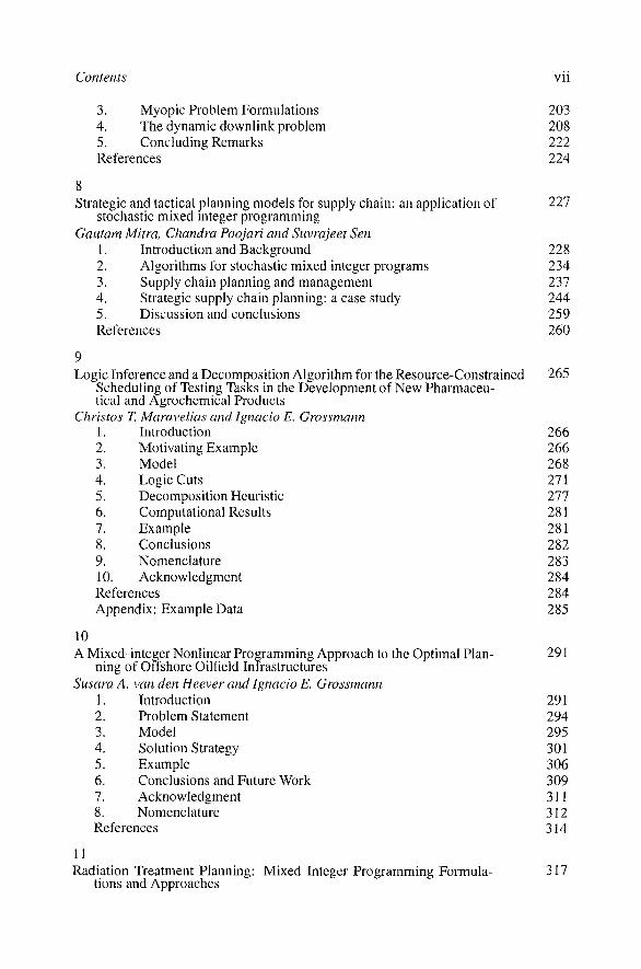
Contents vii
3. Myopic Problem Formulations 203 4. The dynamic downlink problem 208 5. Concluding Remarks 222 References 224
Strategic and tactical planning models for supply chain: an application of 227 stochastic mixed mteger programming
Gautam Mitra, Chandra Poojari and Suvrajeet Sen 1. Introduction and Background 228 2. Algorithms for stochastic mixed integer programs 234 3. Supply chain planning and management 237 4. Strategic supply chain planning: a case study 244 5. Discussion and conclusions 259 References 260
9 Logic Inference and a Decomposition Algorithm for the Resource-Constrained 265
Scheduling of Testing Tasks in the Development of New Pharmaceutical and Agrochemical Products
Christos T, Maravelias and Ignacio E. Grossmann 266 266 268 271 277 281 281 282 283 284 284 285
10 A Mixed-integer Nonlinear Programming Approach to the Optimal Plan- 291
ning of Onshore Oilfield Infrastructures Susara A, van den Heever and Ignacio E. Grossmann
291 294 295 301 306 309 311 312 314
11 Radiation Treatment Planning: Mixed Integer Programming Formula- 317
tions and Approaches
1. 2. 3. 4. 5. 6. 7. 8. 9. 10.
Introduction Motivating Example Model Logic Cuts Decomposition Heuristic Computational Results Example Conclusions Nomenclature Acknowledgment
References Appendix: Example Data
1. 2. 3. 4. 5. 6. 7. 8.
Introduction Problem Statement Model Solution Strategy Example Conclusions and Future Work Acknowledgment Nomenclature
References

viii HANDBOOK ON MODELLING FOR DISCRETE OPTIMIZATION
Michael C. Ferris, Robert R. Meyer and Warren D 'Souza 1. Introduction 318 2. Gamma Knife Radiosurgery 321 3. Brachytherapy Treatment Planning 327 4. IMRT 331 5. Conclusions and Directions for Future Research 336 References 336
12 Multiple Hypothesis Correlation in Track-to-Track Fusion Management 341 Aubrey B Poore, Sabino M Gadaleta and Benjamin J Slocumb
1. Track Fusion Architectures 344 2. The Frame-to-Frame Matching Problem 347 3. Assignment Problems for Frame-to-Frame Matching 350 4. Computation of Cost Coefficients using a Batch Methodology. 360 5. Summary 368 References 369
13 Computational Molecular Biology 373 Giuseppe Lancia
1. Introduction 373 2. Elementary Molecular Biology Concepts 377 3. Alignment Problems 381 4. Single Nucleotide Polymorphisms 401 5. Genome Rearrangements 406 6. Genomic Mapping and the TSP 412 7. Applications of Set Covering 415 8. Conclusions 417 References 418
Index 427

List of Figures
1.1 A piecewise linear approximation to a non-linear function 8 1.2 The convex hull of a pure IP 12 1.3 The convex hull of a mixed IP 13 1.4 Polytopes with different recession directions 15 1.5 A cutting pattern 20 1.6 Optimal pattern 21 1.7 An integer programme 23 1.8 An integer programme with Gomory cuts 27 1.9 Possible values of an integer variable 28 1.10 The first branch of a solution tree 29 1.11 Solution space of the first branch 29 1.12 Final solution tree 30 3.1 Conversion of F to CNF without additional variables. A
formula of the form (if A /) V G is regarded as having theformGV(iJA/) . 72
3.2 Linear-time conversion to CNF (adapted from [21]). The letter C represents any clause. It is assumed that F does not contain variables xi, X2,.... 73
3.3 The resolution algorithm applied to clause set S 74 3.4 The cardinality resolution algorithm applied to cardinal
ity formula set 5 81 3.5 The 0-1 resolution algorithm applied to set 5 of 0-1 inequalities 85 3.6 An algorithm, adapted from [40], for generating a con
vex hull formulation of the cardinality rule (3.26). It is assumed that a , bj G {0,1} is part of the formulation. The cardinality clause {a^} > 1 is abbreviated a . The procedure is activated by calling it with (3,26) as the argument. 86
5.1 A transit system G with 6 stops 131 5.2 The time-expanded network G 132

HANDBOOK ON MODELLING FOR DISCRETE OPTIMIZATION
5.3 Bipartite flow network 136 5.4 Bipartite flow network associated with Team 3 138 5.5 A constraint graph 141 5.6 Network for assessing probabilities 142 5.7 Revised network for assessing probabilities 144 5.8 DNA sequencing network 145 6.1 The Konigsberg bridges problem 165 6.2 Example for the Frederickson's heuristic does not yield
an optimal solution. 169 6.3 Illustration of procedure SHORTEN 171 6.4 Illustration of procedure DROP 172 6.5 Illustration of procedure ADD 172 6.6 Illustration of procedure 2-OPT 173 6.7 Illustration of procedure PASTE 177 6.8 Illustration of procedure CUT 178 7.1 Feasible region for two users 211 7.2 System events in the time domain for the original state
variable and pre-decision state variable in time periods t andt + 1 214
7.3 Geometrical interpretation of the heuristic used for the embedded IP optimization problem for user i. The next feasible rate to vi is r/" — u{si + ai) 218
7.4 Computational complexity of the LADP, textbook DP, and exhaustive search in a scenario where the outcome space consist of an eight state Markov channel, the arrivals have been truncated to less than twelve packets per user 219
7.5 Computational times of the LADP algorithm in terms of CPU-time as a function of the number of mobile users 222
8.1 A scenario tree 231 8.2 Hierarchy of the supply chain planning 238 8.3 A strategic supply chain network 239 8.4 Supply chain systems hierarchy (source- Shapiro, 1998) 242 8.5 SCHUMANN Models/Data Flow 243 8.6 Influence of time on the strategic decisions 248 8.7 The Lagrangian algorithm 254 8.8 Pseudo Code 1 256 8.9 Best hedged-value of the configuration 258 8.10 The frequency of the configuration selected 258 8.11 The probability weighted objective value of the configuration 259 9.1 Motivating example 267

List of Figures xi
9.2 Different cycles for four tests 273 9.3 Branch & bound tree of motivating example 274 9.4 Incidence matrix of constraints 278 9.5 Decomposition heuristic 280 10.1 Configuration of fields, well platforms and production
platforms (Iyer et al, 1998) 292 10.2 Logic-based OA algorithm 303 10.3 Iterative aggregation/disaggregation algorithm 306 10.4 Results 308 10.5 The final configuration 309 10.6 The optimal investement plan 310 10.7 Production profile over six years 310 11.1 The Gamma Knife Treatment Unit. A focusing helmet is
attached to the frame on the patient's head. The patient lies on the couch and is moved back into the shielded treatment area 321
11.2 Underdose of target regions for (a), (c) the pre-treatment plan and (b), (d) the re-optimized plan, (a) and (b) show the base plane, while (c) and (d) show the apex plane 332
12.1 Diagrams of the (a) hierarchical architecture without feedback, (b) hierarchical architecture with feedback, and (c) fully distributed architecture. S-nodes are sensor/tracker nodes, while F-nodes are system/fusion nodes 344
12.2 Diagram showing the sensor-to-sensor fusion process 346 12.3 Diagram showing the sensor-to-system fusion process 347 12.4 Illustration of source-to-source track correlation 349 12.5 Illustration of frame-to-frame track correlation 350 12.6 Illustration of two-dimensional assignment problem for
frame-to-frame matching 352 12.7 Illustration of three-dimensional assignment problem for
frame-to-frame matching 354 12.8 Illustration of multiple hypothesis, multiple frame, cor
relation approach to frame-to-frame matching 357 12.9 Detailed illustration of multiple hypothesis, multiple frame,
correlation approach to frame-to-frame matching 358 12.10 Illustration of sliding window for frame-to-frame matching 360 12.11 Illustration of the batch scoring for frame-to-frame matching 365 13.1 Schematic DNA replication 378 13.2 (a) A noncrossing matching (alignment), (b) The di
rected grid. 382

xii HANDBOOK ON MODELLING FOR DISCRETE OPTIMIZATION
13.3 Graph of RNA secondary structure 3 91 13.4 (a) An unfolded protein, (b) After folding, (c) The con
tact map graph. 395 13.5 An alignment of value 5 396 13.6 A chromosome and the two haplotypes 401 13.7 A SNP matrix M and its fragment conflict graph 403 13.8 Evolutionary events 407

List of Tables
3.1 Prime implications and convex hull formulations of some simple propositions. The set of prime implications of a proposition can serve as a consistent formulation of that proposition. 78
3.2 Catalog of logic-based constraints 98 3.3 Advantages of consistent and tight formulations 99 4.1 A pair of OLS of order 4 107 5.1 A system of routes and stops 131 5.2 Possible locations for amplifiers 134 5.3 Revenues Vij and costs Q 135 5.4 Current team rankings 137 5.5 Games remaining to be played 138 5.6 History of requests allocated to frames 147 5.7 An optimal assignment of requests 148 5.8 Another optimal assignment of requests 148 6.1 Solution values produced by several TS heuristics on
the fourteen CMT instances. Best known solutions are shown in boldface. 164
7.1 Analysis on the performance of different algorithms 223 8.1 Applications of SMIPs 233 8.2 Configuration generation 249 8.3 Dimension of the strategic supply chain model 251 8.4 The stochastic metrics 257 9.1 Model statistics of test problems 272 9.2 Addition of cycle-breaking cuts: Number of constraints
and LP relaxation 272 9.3 Testing data for the motivating example 273 9.4 Income data for the motivating example. 273 9.5 Preprocessing algorithm (PPROCALG) 274
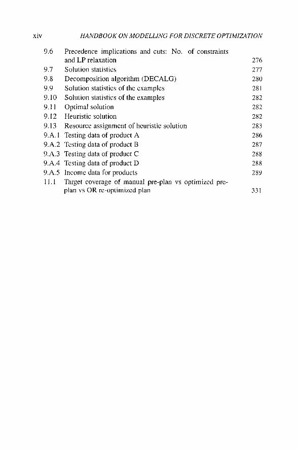
xiv HANDBOOK ON MODELLING FOR DISCRETE OPTIMIZATION
9.6 Precedence implications and cuts: No. of constraints and LP relaxation 276
9.7 Solution statistics 277 9.8 Decomposition algorithm (DECALG) 280 9.9 Solution statistics of the examples 281 9.10 Solution statistics of the examples 282 9.11 Optimal solution 282 9.12 Heuristic solution 282 9.13 Resource assignment of heuristic solution 283 9.A.1 Testing data of product A 286 9.A.2 Testing data of product B 287 9.A.3 Testing data of product C 288 9.A.4 Testing data of product D 288 9.A.5 Income data for products 289 11.1 Target coverage of manual pre-plan vs optimized pre
plan vs OR re-optimized plan 331

Contributing Authors
Gautam Appa Department of Operational Research London School of Economics, London United Kingdom [email protected]
Vasilis Friderikos Centre for Telecommunications Research King's College London United Kingdom [email protected]
Stanislav Busygin Department of Industrial and Systems Engineering, University of Florida 303 Weil Hall, Gainesville FL 32611 USA
busygin @uf I.edu
Sabino M. Gadaleta Numeric a PO Box 271246 Fort Collins, CO 80527-1246 USA
Jean-Fran9ois Cordeau Canada Research Chair in Distribution Management and GERAD, HEC Montreal 3000 chemin de la Cdte-Sainte-Catherine Montreal, Canada H3T2A7 cordeau @crt.umontreal.ca
Ignacio E. Grossmann Department of Chemical Engineering Carnegie Mellon University, Pittsburgh PA 15213, USA
Warren D'Souza University of Maryland School of Medicine 22 South Green Street Baltimore, MD 21201 USA
wdsouOOl @ umaryland.edu
Susara A. van den Heever Department of Chemical Engineering Carnegie Mellon University, Pittsburgh PA 15213, USA
Michael C. Ferris Computer Sciences Department University of Wisconsin 1210 West Dayton Street, Madison Wl 53706, USA
John N. Hooker Graduate School of Industrial Administration Carnegie Mellon University, PA 15213 USA [email protected]

XVI HANDBOOK ON MODELLING FOR DISCRETE OPTIMIZATION
Giusseppe Lancia Dipartimento di Matematica e Informatica Universita di Udine Via delle Scienze 206, 33100 Udine Italy
Gilbert Laporte Canada Research Chair in Distribution Management and GERAD, HEC Montreal 3000 chemin de la Cbte-Sainte-Catherine Montreal, Canada H3T2A7 [email protected]
Dimitris Magos Department of Informatics Technological Educational Institute of Athens 12210 Athens, Greece
Christos T. Maravelias Department of Chemical and Biological Engineering, University of Wisconsin 1415 Engineering Drive, Madison, WI53706-1691, USA
Robert R. Meyer Computer Sciences Department University of Wisconsin 1210 West Dayton Street, Madison WI 53706, USA
Gautam Mitra CARISMA School of Information Systems, Computing and Mathematics, Brunei University, London United Kingdom [email protected]
loannis Mourtos Department of Economics University ofPatras, 26500 Rion, Patras Greece
imourtos @ upatras.gr
Katerina Papadaki Department of Operational Research London School of Economics, London United Kingdom [email protected]
Panos Pardalos Department of Industrial and Systems Engineering, University of Florida 303 Weil Hall, Gainesville FL 32611 USA [email protected]
Leonidas Pitsoulis Department of Mathematical and Physical Sciences, Aristotle University of Thessaloniki, 54124 Thessaloniki, Greece [email protected]
Chandra Poojari CARISMA School of Information Systems, Computing and Mathematics Brunei University, London United Kingdom [email protected]
Aubrey Poore Department of Mathematics Colorado State University Fort Collins, 80523, USA [email protected]

Contributing Authors xvn
Oleg A Prokopyev Department of Industrial and Systems Engineering, University of Florida 303 Weil Hall, Gainesville FL 32611 USA [email protected]
Suvrajeet Sen Department of Systems and Industrial Engineering , University of Arizona, Tuscon,AZ 85721 USA
Douglas R. Shier Department of Mathematical Sciences Clemson University, Clemson,
SC 29634-0975 USA
Benjamin J, Slocumb Numeric a PO Box 271246 Fort Collins, CO 80527-1246 USA
H. Paul Williams Department of Operational Research London School of Economics, London United Kingdom [email protected]

Preface
The primary reason for producing this book is to demonstrate and communicate the pervasive nature of Discrete Optimisation. It has applications across a very wide range of activities. Many of the applications are only known to specialists. Our aim is to rectify this.
It has long been recognized that ''modelling" is as important, if not more important, a mathematical activity as designing algorithms for solving these discrete optimisation problems. Nevertheless solving the resultant models is also often far from straightforward. Although in recent years it has become viable to solve many large scale discrete optimisation problems some problems remain a challenge, even as advances in mathematical methods, hardware and software technology are constantly pushing the frontiers forward.
The subject brings together diverse areas of academic activity as well as diverse areas of applications. To date the driving force has been Operational Research and Integer Programming as the major extention of the well-developed subject of Linear Programming. However, the subject also brings results in Computer Science, Graph Theory, Logic and Combinatorics, all of which are reflected in this book.
We have divided the chapters in this book into two parts, one dealing with general methods in the modelling of discrete optimisation problems and one with specific applications. The first chapter of this volume, written by Paul Williams, can be regarded as a basic introduction of how to model discrete optimisation problems as Mixed Integer Programmes, and outlines the main methods of solving them.
Chapter 2, written by Pardalos et al., deals with the intriguing relationship between the continuous versus the discrete approach to optimisation problems. The authors in chapter 2 illustrate how many well known hard discrete optimisation problems can be modelled and solved by continuous methods, thereby giving rise to the question of whether or not the discrete nature of the problem is the true cause of its computational complexity or the presence of noncon-vexity.
Another subject of great relevance to modelling is Logic. This is covered in chapter 3. The author, John Hooker, describes the relationship with an alter-

XX HANDBOOK ON MODELLING FOR DISCRETE OPTIMIZATION
native solution (and modelling) approach known as Constraint Satisfaction or, as it is sometimes called, Constraint Logic Programming. This approach has emerged more from Computer Science than Operational Research. However, the possibility of "hybrid methods" based on combining the approaches is on the horizon, and has been realized with some problem specific implementations.
In chapter 4 Appa et al. illustrate how discrete optimisation modelling and solution methods can be applied to answer questions regarding a problem arising from combinatorial mathematics. Specifically the authors present various optimisation formulations of the mutually orthogonal latin squares problem, from constraint programming (which is covered in detail in chapter 3) to mixed integer programming formulations and matroid intersection, all of which can be used to answer existence questions for the problem.
It has long been established that Networks can model most of today's complex systems such as transportation systems, telecommunication systems, and computer networks to name a few, and network optimisation has proven to be a valuable tool in analyzing the behavior of these systems for design purposes. Chapter 5 by Shier enhances further the applicability of network modelling by presenting how it can also be applied to less apparent systems ranging from genomics, sports and artificial intelligence.
Chapter 6 is the last chapter in the methods part of the book, where Cordeau and Laporte discuss a class of problems known as vehicle routing problems. Vehicle routing problems enjoy a plethora of applications in the transportation and logistics sector, and the authors in chapter 6 present the state of the art with respect to exact and heuristic methods for solving them.
In the second part of the book various real life applications are presented, most of them formulated as mixed integer linear or nonlinear programming problems. Chapter 7 by Papadaki and Friderikos, is concerned with the solution of optimization problems arising in resource management problems in wireless cellular systems by employing a novel approach, the so called approximate dynamic programming.
Most of the discrete optimisation models presented in this book are of deterministic nature, that is the values of the input data are assumed to be known with certainty. There are however real life applications where such an assumption is inapplicable, and stochastic models need to be considered. This is the subject of chapter 8, by Mitra et al. where stochastic mixed integer programming models are discussed for supply chain management problems.
In chapters 9 and 10 Grossmann et al. present how discrete optimisation modeling can be efficiently applied to two specific application areas. In chapter 9 mixed integer linear programming models are presented for the problem of scheduling regulatory tests of new pharmaceutical and agrochemical products, while in chapter 10 a mixed integer nonlinear model is presented for the

PREFACE xxi
optimal planning of offshore oilfield infrastructures. In both chapters the authors also present solution techniques.
Optimization models to radiation therapy for cancer patients is the subject discussed in chapter 11 by Ferris and Meyer. They show how the problem of irradiating patients for treatment of cancerous tumors can be formulated as a discrete optimisation problem and can be solved as such.
In chapter 12 the data association problem that arises in target tracking is considered by Poore et al. The objective in this chapter is to partition the data that is created by multiple sensors observing multiple targets into tracks and false alarms, which can be formulated as a multidimensional assignment problem, a notoriously difficult integer programming problem which generalizes the well known assignment problem.
Finally chapter 13 is concerned with the life sciences, and Lancia shows how some challenging problems of Computational Biology can now be solved as discrete optimisation models.
Assembling and planning this book has been much more of a challenge than we at first envisaged. The field is so active and diverse that it has been difficult covering the whole subject. Moreover the contributors have themselves been so deeply involved in practical applications that it has taken longer than expected to complete the volume.
We are aware that, within the limits of space and the time of contributors we have not been able to cover all topics that we would have liked. For example we have been unable to obtain a contributor on Computer Design, an area of great importance, or similarly on Computational Finance and Air Crew Scheduling. By way of mitigation we are pleased to have been able to bring together some relatively new application areas.
We hope this volume proves a valuable work of reference as well as to stimulate further successful applications of discrete optimisation.
GAUTAM APPA, LEONIDAS PITSOULIS, H. PAUL WILLIAMS

xxii HANDBOOK ON MODELLING FOR DISCRETE OPTIMIZATION
Acknowledgments We would like to thank the contributing authors of this volume, and the
many anonymous referees who have helped us review the chapters all of which have been thoroughly refereed. We are also thankful to the staff of Springer, in particular Gary Folven and Carolyn Ford, as well as the series editor Fred Hillier.
Paul Williams acknowledges the help which resulted from Leverhulme Research Fellowship RF&G/9/RFG/2000/0174 and EPSRC Grant EP/C530578/1 in preparing this book.

I
METHODS
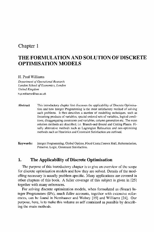
Chapter 1
THE FORMULATION AND SOLUTION OF DISCRETE OPTIMISATION MODELS
H. Paul Williams Department of Operational Research London School of Economics, London United Kingdom [email protected]
Abstract This introductory chapter first discusses the applicability of Discrete Optimisation and how Integer Programming is the most satisfactory method of solving such problems. It then describes a number of modelling techniques, such as linearisng products of variables, special ordered sets of variables, logical conditions, disaggregating constraints and variables, column generation etc. The main solution methods are described, i.e. Branch-and-Bound and Cutting Planes. Finally alternative methods such as Lagrangian Relaxation and non-optimising methods such as Heuristics and Constraint Satisfaction are outlined.
Keywords: Integer Programming, Global Optima, Fixed Costs,Convex Hull, Reformulation, Presolve, Logic, Constraint Satisfaction.
1. The Applicability of Discrete Optimisation The purpose of this introductory chapter is to give an overview of the scope
for discrete optimisation models and how they are solved. Details of the modelling necessary is usually problem specific. Many applications are covered in other chapters of this book. A fuller coverage of this subject is given in [25] together with many references.
For solving discrete optimization models, when formulated as (linear) Integer Programmes (IPs), much fuller accounts, together with extensive references, can be found in Nemhauser and Wolsey [19] and Williams [24]. Our purpose, here, is to make this volume as self contained as possible by describing the main methods.

4 HANDBOOK ON MODELLING FOR DISCRETE OPTIMIZATION
Limiting the coverage to linear IPs should not be seen as too restrictive in view of the reformulation possibilities described in this chapter.
It is not possible, totally, to separate modelling from the solution methods. Different types of model will be appropriate for different methods. With some methods it is desirable to modify the model in the course of optimisation. These two considerations are addressed in this chapter.
The modelling of many physical systems is dominated by continuous (as opposed to discrete) mathematics. Such models are often a simplification of reality, but the discrete nature of the real systems is often at a microscopic level and continuous modelling provides a satisfactory simplification. What's more, continuous mathematics is more developed and unified than discrete mathematics. The calculus is a powerful tool for the optimisation of many continuous problems. There are, however, many systems where such models are inappropriate. These arise with physical systems (e.g. construction problems, finite element analysis etc) but are much more common in decision making (operational research) and information systems (computer science). In many ways, we now live in a 'discrete world'. Digital systems are tending to replace analogue systems.
2. Integer Programming
The most common type of model used for discrete optimisation is an Integer Programme (IP) although Constraint Logic Programmes (discussed in the chapter by Hooker) are also applicable (but give more emphasis to obtaining feasible rather than optimal solutions). An IP model can be written:
Maximise/Minimise c 'x-i-d 'y (1.1)
Subject to: A x + B y < b (L2)
xe3f t ,yGZ (L3)
X are (generally non-negative) continuous variables and y are (generally non-negative and bounded) integer variables.
If there are no integer variables we have a Linear Programme (LP). If there are no continuous variables we have a Pure IP (PIP). In contrast the above model is known as a Mixed IP (MIP). Most practical models take this form. It should be remarked that although the constraints and objective of the above model are linear this is not as restrictive, as it might seem. In IP, nonlinear expressions can generally be linearised (with possibly some degree of approximation) by the addition of extra integer variables and constraints. This is explained in this chapter. Indeed IP models provide the most satisfactory way of solving, general non-linear optimisation problems, in order to obtain a global (as opposed to local) optimum. This again is explained later in this chapter.

The Formulation and Solution of Discrete Optimisation Models 5
LPs are 'easy' to solve in a well defined sense (they belong to the complexity class P). In contrast, IPs are difficult, unless they have a special structure, (they are in the NP - complete complexity class). There is often considerable scope for formulating, or reformulating, IP models in a manner which makes them easier to solve.
3. The Uses of Integer Variables The most obvious use of integer variables is to model quantities which can
only take integer values e.g. numbers of cars, persons, machines etc. While this may be useful, if the quantities will always be small integers (less than, say, 10), it is not particularly common. Generally such quantities would be represented by continuous variables and the solutions rounded to the nearest integer.
3.1 0-1 Variables More commonly integer variables are restricted to two values, 0 or 1 and
known as 0-1 variables or binary variables. They then represent Yes/No decisions (e.g. investments). Examples of their use are given below. Before doing this it is worth pointing out that any bounded integer variable can be represented as a sum of 0-1 variables. The most compact way of doing this is to use a binary expansion of the coefficients. Suppose e.g. we have an integer variable y such that:
0 < y < [/ (1.4)
Where U is an upper bound on the value of y. Create 0-1 variables:
2/0 , yi , 2/2 , . . . 2/Liog2 u\
then y can be represented by:
2/0 + 2yi + 47/2 + + 2L -S2 ^\yy^os2 u\ (1.5)
3.1.1 Fixed Charge Problems. A very common use of 0-1 variables is to represent investments or decisions which have an associated fixed cost (/). If carried out, other continuous variables xi, X2,. . . , Xn bringing in e.g. variable profits Pi^P2,'",Pn come into play. This situation would be modelled as:
Maximise YlPj^j — fv (1.6)
Subject to: ^Xj - My < 0 (1.7) j
(and other constraints)

6 HANDBOOK ON MODELLING FOR DISCRETE OPTIMIZATION
where M represents an upper bound on the combined level of the continuous activities.
If y =: 0 (investment not made) all the x^are forced to zero. On the other hand \f y — \ (investment is made) the fixed cost f is incurred but the Xj can take positive values and profit is made.
There are, of course, many extensions to this type of model where alternative or additional investments can be made, etc. The basic idea is, however, the same.
3.1.2 Indicator Variables. A very powerful modelling technique is to use 0-1 variables to distinguish situations which are ('discretely') different. If there is a simple dichotomy then the two possible values of a 0-1 variable can be used to make the distinction. For example, suppose we want to model the condition
Y^ai jXj < 6i or /J<^2j^j ^ ^2 (1-8) J 3
Such a condition is known as a disjunction of constraints (in contrast to the usual LP conjunction of constraints). Let y = 0 impose the first constraint in the disjunction and y= 1 impose the second constraint. This is achieved by the following conjunction of constraints
Y^aijXj-Miy<hi (1.9)
j
^a2jXj + M2y <M2 + b2 (1.10)
j
Ml is an upper bound on the value of the expression J2 ^ij^j "~ ^i ^^d M2 an j
upper bound on CL2JXJ — 62. (If either of the expressions has no upper bound j
then the disjunction can only be modelled in special conditions.) There is an alternative and preferable way of modelling this condition which is considered later in this chapter.
Should a disjunction of more than two constraints be needed then more than one 0 - 1 variable can be used. For example the situation
2^ciijXj < 61 or ^<^2j^j <b2 or . . . or ^^^(^nj^j ^K (1.11) j j j
can be modelled as ^aijXj-Miyi <6i (1.12)
j
Y^a2jXj-M2y2<h2 (1.13)

The Formulation and Solution of Discrete Optimisation Models 7
Y^ anjXj - MnVn < K (1.14)
3
yi + y2 + '" + yn<n-l (1.15)
The situation where at least A: of a given set of constraints [l <k <n) hold can easily be modelled by amending (1.15).
There are many situations where one wishes to model such disjunctions. For example:
• This operation must finish before the other starts or vice versa;
• We must either not include this ingredient or include it above a given threshold level.
• At least (most) A: of a given set of possible warehouses should be built.
In fact all of IP could be reduced to disjunctions of linear constraints. This is only a useful paradigm for some problems. However the modelling of disjunctive conditions has been thoroughly analysed in Balas [2].
3.2 Special Ordered Sets of Variables (Discrete Entities) If a quantity can take a number of discrete values then a convenient method
of modelling is a Special Ordered Set of Type 7 (SI set). Suppose we wish to model a quantity which can take values ai, a2 , . . . , a^. We would represent this quantity by
X = aiyi + a2y2 + • • • + anyn (1.16)
and with the constraint
yi + y2 + — \ - yn = i
with the stipulation that
Exactly one member of the set {2/1, 2? * • * 5 ^n} c^^ be non-zero
Note that it is not necessary to stipulate that the yj variables be integer and 0-1. An S1 set (as opposed to the individual variables in it) should be regarded
as a discrete entity. It can be considered as a generalisation of a general integer variable where values are not evenly spaced. SI sets are regarded as entities analogous to integer variables when the Branch-and Bound algorithm, described later in this chapter, is used.
A variant of SI sets are Special Ordered sets of Type 2 (S2 sets). These are widely used to model non-linear functions. In order to model a non-linear function it must be separated into the sum of non-linear functions of a single variable. This can generally be done by introducing new variables and constraints. (The possibility of doing this goes back to one of Hilbert's problems.)

HANDBOOK ON MODELLING FOR DISCRETE OPTIMIZATION
AX)
A^
A^
Figure L1. A piecewise linear approximation to a non-linear function
Each non-linear function of a single variable is approximated by a piecewise linear function i.e. a series of linear segments as illustrated in Figure 1.1. A grid value is defined for the relevant values of the argument x (not necessarily evenly spaced) and the function f{x) defined at those values. We define an S2 s t {yi , ^2) ••• 1/5} with the constraints
X = Xiyi + X2y2 + Xs 7/3 + X4 7/4 + X5 2/5 (1.17)
f{x) - f{Xi)yi + f{X2)y2 + f{X^)y^ + f{X^)y^ + f{X^)y^ (1.18)
yi + y2 + 2/3 + 2/4 + ys = 1 (1.19)
together with the stipulation that
At most two adjacent j/5 can be non-zero
Note that the yj are continuous. If, for example, yz — \^yA — \ (implying the other 2/j=0) this corresponds to the point A in Figure 1.1. By this means, only the points on one of the straight-line segments in Figure 1.1 are represented by(x, f {x)). Clearly a more refined grid can give a more accurate approximation to a function (at the expense of more variables).
The concept of Special Ordered Sets are described by [3] with an extension to deal with functions of more than one variable in [4]. There are, of course, alternative methods of modelling condition (1.11) using 0-1 variables since we again have a disjunction of possibilities. However, using Special Ordered Sets has computational advantages when using the Branch-and-Bound algorithm.

The Formulation and Solution of Discrete Optimisation Models 9
4. The Modelling of Common Conditions 4.1 Products of Variables
It has already been remarked that non-linear expressions can be reformulated using linear constraints involving integer variables. A common non-linearity is products of integer variables. As explained above (bounded) general integer variables can always be expressed using 0-1 variables. Therefore we confine our attention to products of 0-1 variables.
Consider the product yi y2 which we will represent by a new variable z where yi and 2/2 ar^ 0-1 variables. This product itself can only take values 0 or 1 depending on the values of yi and ^2- If cither is zero the product itself is 0. Otherwise it is 1.
Logically we have
yi = 0 or 2/2 = 0 (or both) implies z = 0
This can be modelled by yi + y2-2z>0 (1.20)
(There is a 'better' way of modelling this which will be given later in this chapter.) We also have to model
yi = I and 2/2 == 1 implies z = 1.
This can be modelled by yi + y2-z<i (1.21)
If we have a product of 3 or more 0 - 1 variables then we can repeat the above formulation procedure.
A product of a continuous variable x and a 0-1 variable y can be represented by a continuous variable z. The variable z will then be equal to x or to zero depending on whether y is 1 or 0. Either way we have
z-x<0 (1.22)
If y =^ 1 then we want the condition z — x. This may be done by modelling the condition
y — 1 implies z > x
since, together with (1.22), this would imply z = x. We can model the condition as
X- z + My<M (1.23)
M must be chosen as a suitably large number (an upper bound) which x (and therefore z) will not exceed.
If we wish to model the product of an 0-1 variable and an expression this formulation can be extended in an economical manner, as done by Glover [10].

10 HANDBOOK ON MODELLING FOR DISCRETE OPTIMIZATION
4.2 Logical Conditions The common use of 0-1 variables in IP models suggests the analogy with
modelling of True/False propositions which forms the subject matter of the Propositional Calculus (Boolean Algebra). This close relationship is explored further in this book in Chapter 3 by Hooker. Here we give a taste for the power of IP to model the relationships of the Propositional Calculus.
In IP (and LP) our propositions are constraints which may be true or false. (An LP model consists of a conjunction of constraints i.e. they must all be true). We can represent the truth or falsity of a constraint by the setting of a 0-1 variable. If, for example, we have the constraint
^aj Xj < b (1.24) j
then we can incorporate the 0-1 variable y into the constraint to give
^ ajXj -\- My < M -\-b (1.25) j
where M is an upper bound on the expression
2_]cijXj — b (1.26) j
If y = 1 the constraint (1.24) is forced to hold. If y == 0 it becomes vacuous. Sometimes we may wish to model the condition
y ^ ajXj < b implies y = 1 3
This can be represented by its equivalent contrapositive statement
2/ == 0 implies y^ajXj > b (1-27) j
Since it is conventional only to use non-strict inequalities we can replace
Y^ajXj >b j
by "^ajXj >b + e (1.28)
j
where e is a suitable small positive number. Now (1.27) can be modelled (by analogy with (1.25)) as
^ ajXj + my>b + e (1.29)

The Formulation and Solution of Discrete Optimisation Models 11
where m is a lower bound on the expression
3
It is now possible to model the standard connectives of the Propositional Calculus applied to constraints by means of (in)equalities between 0-1 variables.
We have already modelled the 'or' condition by constraints (1.9) and (1.10) and (1.12) to (1.15). The 'and' condition is simply modelled by repeating the constraints (as in LP). The implies' condition is modelled thus:
2/i == 1 implies 2/2 = 1
is represented by yi — ^2 ^ 0
We now have all the machinery for modelling logical conditions which will be explained in greater depth in Hooker's chapter (see chapter 3).
5. Reformulation Techniques Despite advances in methods of solving Discrete Optimisation problems, as
well as the dramatic increase in the speed and storage capacity of computers, many such problems still remain very difficult to solve. There is, however, often great flexibility in the way such problems are modelled as Integer Programmes. It is frequently possible to remodel a problem in a way which makes it easier to solve. This is the subject of this section.
5.1 The Convex Hull of Integer Solutions The constraints of a Linear Programme (LP) restrict the feasible solutions to
a set which can be represented by a Polytope in multidimensional space. For Integer Programmes the set is further restricted to the lattice of integer points within a Polytope. This is illustrated, in Figure 1.2, by the constraints of a 2-Variable IP, which can therefore be represented in 2-dimensional space.
- x i + 2rz;2 < 7 (1.30)
xi + 3x2 < 15 (1.31)
7x1-3x2 < 23 (1.32)
3^b^2 ^ 0 and integer (1.33)
The boundaries of constraints (1.30), (1.31) and (1.32) are represented by the lines AB, BC and CD respectively and the non-negativity conditions by OA and OD. However, the integrality restrictions on xi and X2 restrict us further to the lattice of points marked. If we were to ignore the integrality conditions then, given an objective function, we would have an LP model. An optimal

12 HANDBOOK ON MODELLING FOR DISCRETE OPTIMIZATION
Figure 1.2. The convex hull of a pure IP
solution would lie at one of the vertices O, A, B, C, or D (if there were alternative solutions some of them would be between these vertices). The LP got by ignoring the integrality conditions is known as the "LP Relaxation" of the model.
However, if we were to represent the constraints whose boundaries are the bold lines we would have a more constrained LP problem whose solutions would be O, P, Q, R, S, T or U which would satisfy the integrality requirements. The region enclosed in the bold lines is known as the Convex Hull of Feasible Integer Solutions. It is the smallest convex set containing the feasible integer solutions. For this example the constraints defining the convex hull are:
-Xi +X2
X2
Xi +X2
x\
1X\ — X2
X\,X2
<
<
<
<
<
>
3 4
7 4
6
0
(1.34)
(L35)
(L36)
(1.37)
(1.38)
(1.39)
Computationally LP models are much easier to solve than IP models. Therefore reformulating an IP by appending or substituting ihtst facet defining constraints would appear to make a model easier to solve. With some types of model it is fairly straightforward to do this. In general, however, the derivation of facet defining constraints is extremely difficult and there is no known systematic way of doing it. What is more, there are often an astronomic number of facets making it impossible to represent them all with limited computer storage.


![[Vehicle Routing and Transportation 3] - Universiteit Hasselt · [Vehicle Routing and Transportation 3] D16 ... Algorithm for the Multi-Objective Vehicle Routing Problem with Time](https://img.dokumen.tips/doc/110x75/5acb82947f8b9aa3298e93a2/vehicle-routing-and-transportation-3-universiteit-hasselt-vehicle-routing-and.jpg)


