Evolutionary Algorithms for Vehicle Routing · PDF fileEvolutionary Algorithms for Vehicle Routing Problems ... Evolutionary Algorithms for Vehicle Routing Problems ... TS Osman 1993

Evolutionary Algorithms for Vehicle Routing Problems – Christian Prins - Slide #1

Evolutionary Algorithms for Vehicle Routing Problems

Christian PRINS

Institute Charles Delaunay, FRE CNRS 2848 University of Technology of Troyes (UTT), France

[email protected]

Spring School on Vehicle Routing Avignon, 27-28/03/2008


Outline

1. Genetic and memetic algorithms 2. Application to the Vehicle Routing Problem (VRP) 3. MA|PM and the Heterogeneous Fleet VRP (HFVRP) 4. The Periodic VRP (PVRP).


PART 1

Genetic and Memetic Algorithms (GA and MA)


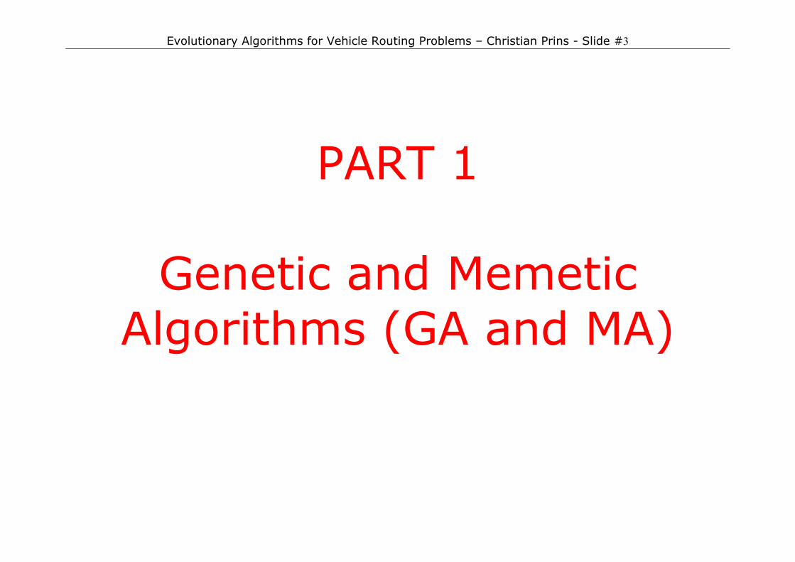
Classical GA – Incremental version 1: initialize population Pop 2: repeat 3: select two parents P1, P2 from Pop 4: crossover P1 ⊗ P2 → C1, C2 5: for each child C do 6: mutate C (small probability) 7: replace one solution B in Pop by C 8: endfor 9: until stopping criterion satisfied. Not aggressive enough for combinatorial optimization, Cannot compete with tabu search for instance.


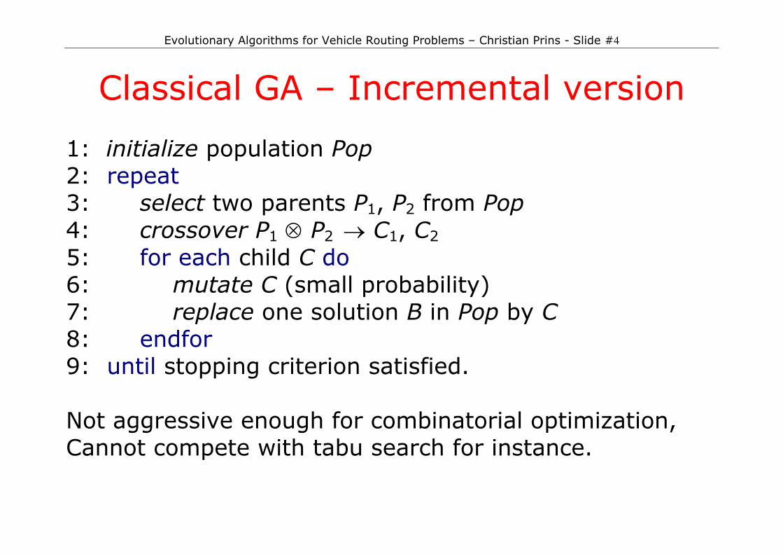
A simple example: the TSP 1/3 Travelling Salesman Problem Data: n nodes, distance matrix D n×n Goal: compute one cycle of minimum total length,

visiting each node once. 1. Chromosome and evaluation

One solution can be coded as a node permutation C. Example: C = (5, 1, 4, 6, 3, 2) The fitness (solution cost) is:

),(),()( 1

1

11 CCDCCDCF n

n

iii +=∑

−

=+


A simple example: the TSP 2/3 2. Initial population Pop of nc chromosomes

Generate nc random permutations, compute their costs.

3. Selection of two parents P1, P2 in Pop

Binary tournament: randomly draw two chromosomes, keep the best as P1. Repeat to get P2.

4. Simple one-point crossover Parent 1: 1 3 9 2|7 4 5 8 6 Parent 2: 8 3 4 7|6 1 9 5 2 Child 1: 1 3 9 2|8 4 7 6 5 Child 2: 8 3 4 7|1 9 2 5 6


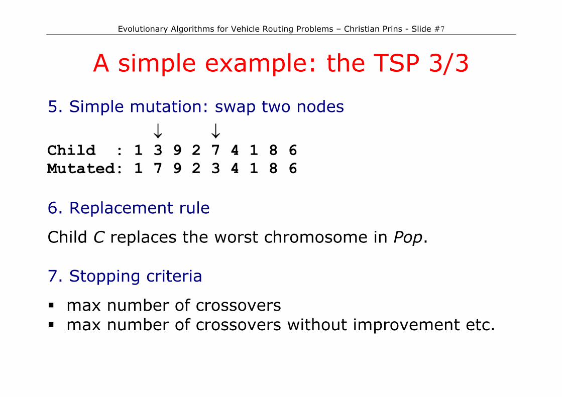
A simple example: the TSP 3/3 5. Simple mutation: swap two nodes

↓ ↓ Child : 1 3 9 2 7 4 1 8 6 Mutated: 1 7 9 2 3 4 1 8 6 6. Replacement rule

Child C replaces the worst chromosome in Pop. 7. Stopping criteria

max number of crossovers max number of crossovers without improvement etc.


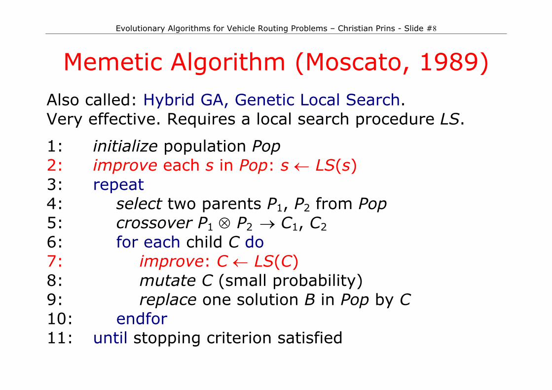
Memetic Algorithm (Moscato, 1989)

Also called: Hybrid GA, Genetic Local Search. Very effective. Requires a local search procedure LS.

1: initialize population Pop 2: improve each s in Pop: s ← LS(s) 3: repeat 4: select two parents P1, P2 from Pop 5: crossover P1 ⊗ P2 → C1, C2 6: for each child C do 7: improve: C ← LS(C) 8: mutate C (small probability) 9: replace one solution B in Pop by C 10: endfor 11: until stopping criterion satisfied


PART 2

The VRP case


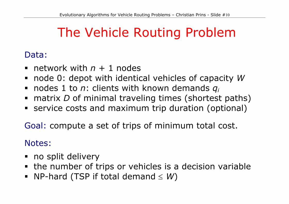
The Vehicle Routing Problem Data:

network with n + 1 nodes node 0: depot with identical vehicles of capacity W nodes 1 to n: clients with known demands qi matrix D of minimal traveling times (shortest paths) service costs and maximum trip duration (optional)

Goal: compute a set of trips of minimum total cost.

Notes:

no split delivery the number of trips or vehicles is a decision variable NP-hard (TSP if total demand ≤ W)


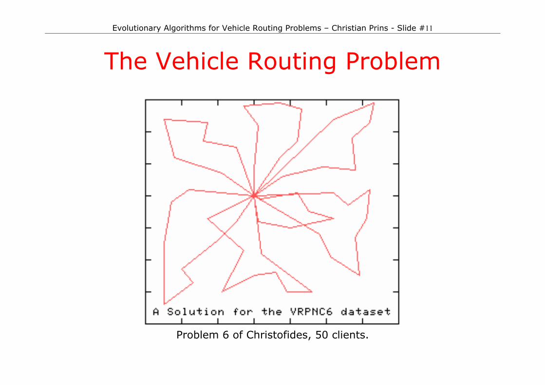
The Vehicle Routing Problem

Problem 6 of Christofides, 50 clients.


Entry points for VRP literature T.A. Crainic, G. Laporte, Fleet management and logistics, Kluwer, 1998.

G. Laporte, M. Gendreau, J.Y. Potvin, F. Semet, Classical and modern heuristics for the VRP, Int. Trans. Oper. Res. 7, 285-300, 2000.

P. Toth, D. Vigo, The vehicle routing problem, SIAM, 2002.

J.F. Cordeau, M. Gendreau, A. Hertz, G. Laporte, J.S. Sormany, New heuristics for the Vehicle Routing Problem. In: A. Langevin and D. Riopel (Eds.), Logistics systems: design and optimization, pp. 279-298, Kluwer, 2005.

J.F. Cordeau, G. Laporte, M.W.P. Savelsbergh, D. Vigo. Vehicle routing. In: C. Barnhart and G. Laporte (Eds.), Transportation, Handbooks in OR-MS, vol. 14, 367-428, Elsevier, 2007.


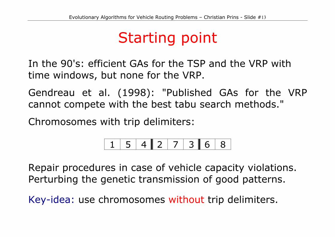
Starting point In the 90's: efficient GAs for the TSP and the VRP with time windows, but none for the VRP.

Gendreau et al. (1998): "Published GAs for the VRP cannot compete with the best tabu search methods."

Chromosomes with trip delimiters:

1 5 4 2 7 3 6 8 Repair procedures in case of vehicle capacity violations. Perturbing the genetic transmission of good patterns.

Key-idea: use chromosomes without trip delimiters.


Chromosome and crossover

A chromosome is a permutation of the n clients. Implicit shortest paths between adjacent clients. No trip delimiters: giant tour for a vehicle with W=∞.

Two TSP crossovers that can be reused (we took OX): LOX random cut-points ↓ ↓ P1 : 1 3 2|6 4 5|9 7 8 P2 : 3 7 8|1 4 9|2 5 6 C : 3 7 8 6 4 5 1 9 2

OX random cut-points ↓ ↓ P1 : 1 3 2|6 4 5|9 7 8 P2 : 3 7 8|1 4 9|2 5 6 C : 8 1 9 6 4 5 2 3 7

But how to get a VRP solution and its cost?


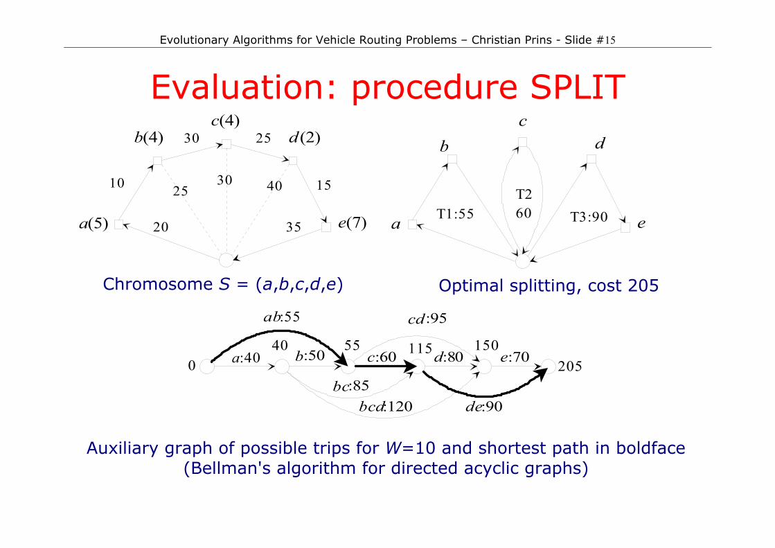
Evaluation: procedure SPLIT

a(5)

b(4)c(4)

d (2)

e(7)

10

30 25

1530 40

35

25

20

Chromosome S = (a,b,c,d,e)

a

bc

d

eT1:55 T3:90T260

Optimal splitting, cost 205

a:40 b:50 c:60 d:80 e:70

ab:55

bc:85bcd:120

cd :95

de:90

040 55 115 150

205

Auxiliary graph of possible trips for W=10 and shortest path in boldface (Bellman's algorithm for directed acyclic graphs)


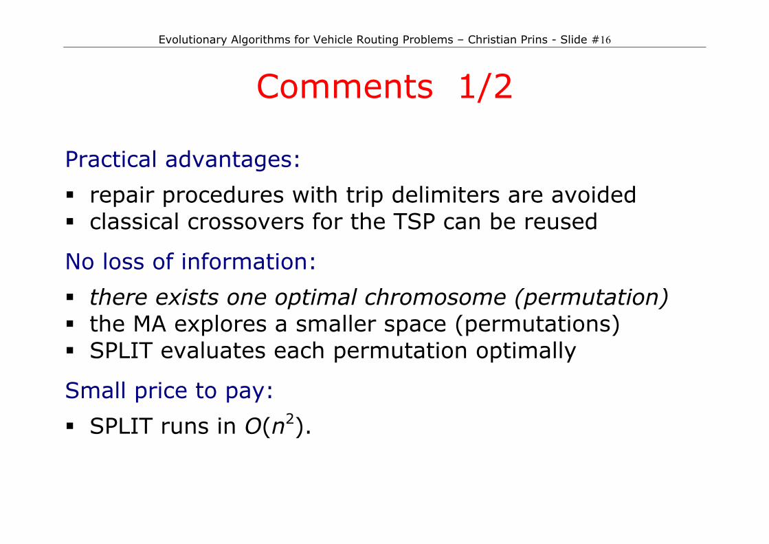
Comments 1/2 Practical advantages:

repair procedures with trip delimiters are avoided classical crossovers for the TSP can be reused

No loss of information:

there exists one optimal chromosome (permutation) the MA explores a smaller space (permutations) SPLIT evaluates each permutation optimally

Small price to pay:

SPLIT runs in O(n2).


Comments 2/2

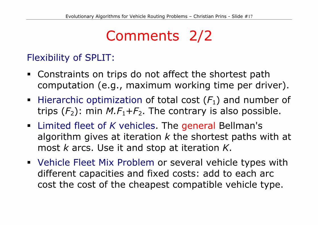
Flexibility of SPLIT:

Constraints on trips do not affect the shortest path computation (e.g., maximum working time per driver).

Hierarchic optimization of total cost (F1) and number of trips (F2): min M.F1+F2. The contrary is also possible.

Limited fleet of K vehicles. The general Bellman's algorithm gives at iteration k the shortest paths with at most k arcs. Use it and stop at iteration K.

Vehicle Fleet Mix Problem or several vehicle types with different capacities and fixed costs: add to each arc cost the cost of the cheapest compatible vehicle type.


Population structure Table Pop of nc distinct chromosomes:

to avoid premature convergence (clones) better dispersal of solutions (better exploration)

A simple cost-spacing rule for a stronger dispersal:

∀ P1, P2 ∈ Pop : |cost(P1) – cost(P2)| ≥ ∆ a child violating this rule is rejected acceptable rejection rate if nc small, e.g. nc = 30

Initial composition of Pop:

3 good solutions obtained by classical VRP heuristics nc-3 random permutations, evaluated by SPLIT


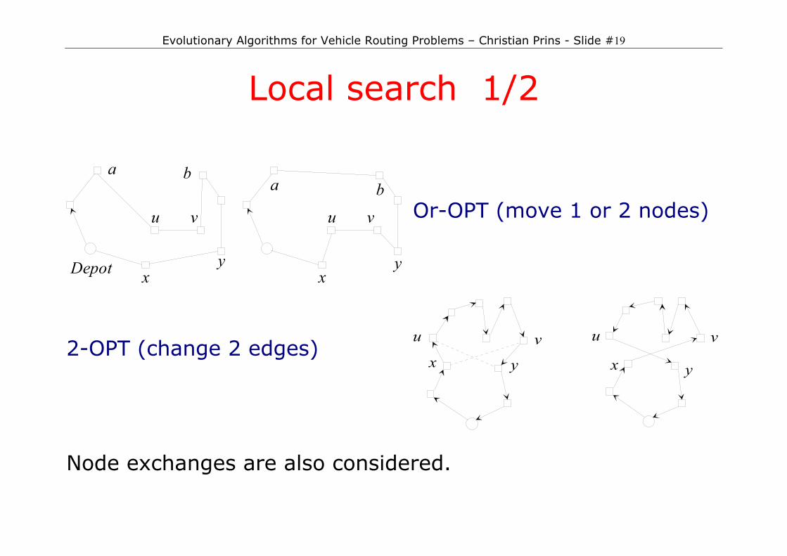
Local search 1/2

v

xyDepot

u v

xy

u

a ba b

Or-OPT (move 1 or 2 nodes)

2-OPT (change 2 edges)

u v u v

x y x y

Node exchanges are also considered.


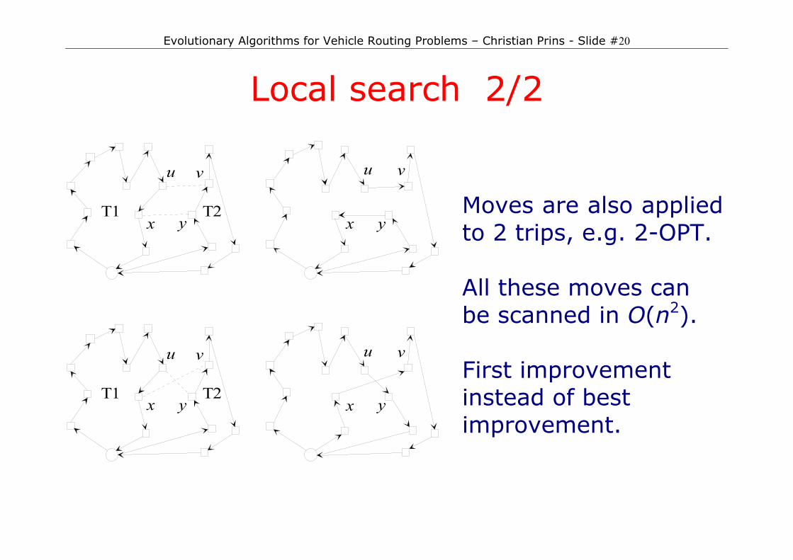
Local search 2/2

u v

x yT1 T2

u v

x y

u v

x yT1 T2

u v

x y

Moves are also applied to 2 trips, e.g. 2-OPT.

All these moves can be scanned in O(n2).

First improvement instead of best improvement.


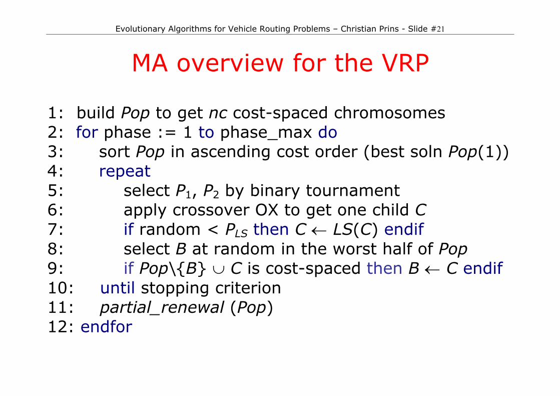
MA overview for the VRP

1: build Pop to get nc cost-spaced chromosomes 2: for phase := 1 to phase_max do 3: sort Pop in ascending cost order (best soln Pop(1)) 4: repeat 5: select P1, P2 by binary tournament 6: apply crossover OX to get one child C 7: if random < PLS then C ← LS(C) endif 8: select B at random in the worst half of Pop 9: if Pop\{B} ∪ C is cost-spaced then B ← C endif 10: until stopping criterion 11: partial_renewal (Pop) 12: endfor


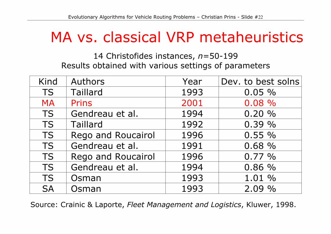
MA vs. classical VRP metaheuristics

14 Christofides instances, n=50-199 Results obtained with various settings of parameters

Kind Authors Year Dev. to best solns TS Taillard 1993 0.05 % MA Prins 2001 0.08 % TS Gendreau et al. 1994 0.20 % TS Taillard 1992 0.39 % TS Rego and Roucairol 1996 0.55 % TS Gendreau et al. 1991 0.68 % TS Rego and Roucairol 1996 0.77 % TS Gendreau et al. 1994 0.86 % TS Osman 1993 1.01 % SA Osman 1993 2.09 %

Source: Crainic & Laporte, Fleet Management and Logistics, Kluwer, 1998.


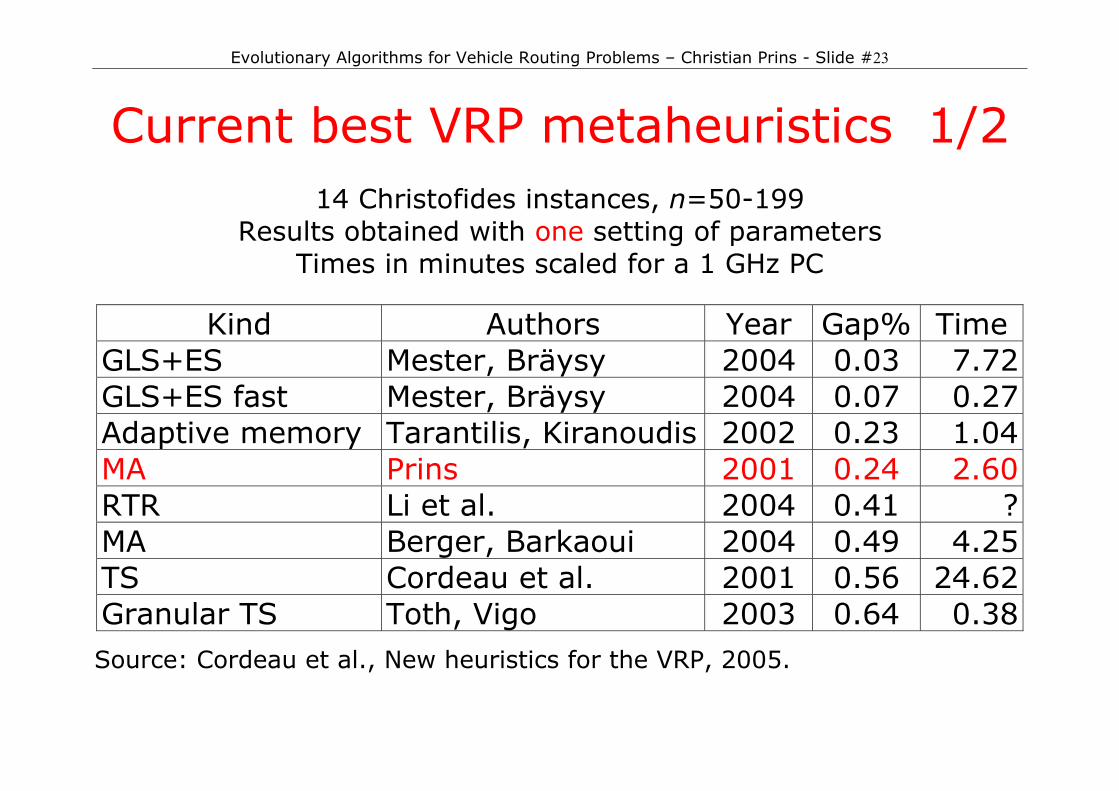
Current best VRP metaheuristics 1/2

14 Christofides instances, n=50-199 Results obtained with one setting of parameters

Times in minutes scaled for a 1 GHz PC

Kind Authors Year Gap% Time GLS+ES Mester, Bräysy 2004 0.03 7.72 GLS+ES fast Mester, Bräysy 2004 0.07 0.27 Adaptive memory Tarantilis, Kiranoudis 2002 0.23 1.04 MA Prins 2001 0.24 2.60 RTR Li et al. 2004 0.41 ? MA Berger, Barkaoui 2004 0.49 4.25 TS Cordeau et al. 2001 0.56 24.62 Granular TS Toth, Vigo 2003 0.64 0.38

Source: Cordeau et al., New heuristics for the VRP, 2005.


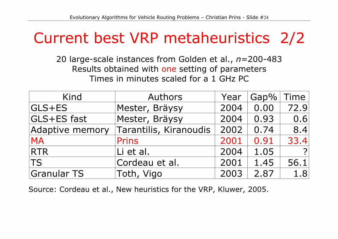
Current best VRP metaheuristics 2/2

20 large-scale instances from Golden et al., n=200-483 Results obtained with one setting of parameters

Times in minutes scaled for a 1 GHz PC

Kind Authors Year Gap% Time GLS+ES Mester, Bräysy 2004 0.00 72.9 GLS+ES fast Mester, Bräysy 2004 0.93 0.6 Adaptive memory Tarantilis, Kiranoudis 2002 0.74 8.4 MA Prins 2001 0.91 33.4 RTR Li et al. 2004 1.05 ? TS Cordeau et al. 2001 1.45 56.1 Granular TS Toth, Vigo 2003 2.87 1.8

Source: Cordeau et al., New heuristics for the VRP, Kluwer, 2005.


Reference C. Prins, A simple and effective evolutionary algorithm for the Vehicle Routing Problem, Computers & Operations Research, 31(12), pp. 1985-2002, 2004. Presented first at MIC 2001.


PART 3

Memetic Algorithms with Population Management

The HVRP case


MA|PM (Sörensen, 2003) General principles

small population of high-quality solutions local improvement diversity controlled via population management

Population management

distance d(x,y) between solutions, in solution space distance to a population P: dP(s) = min {d(s,x): x∈P} a new solution s is added to P if dP(s) ≥ ∆ the diversity parameter ∆ can be dynamically adjusted


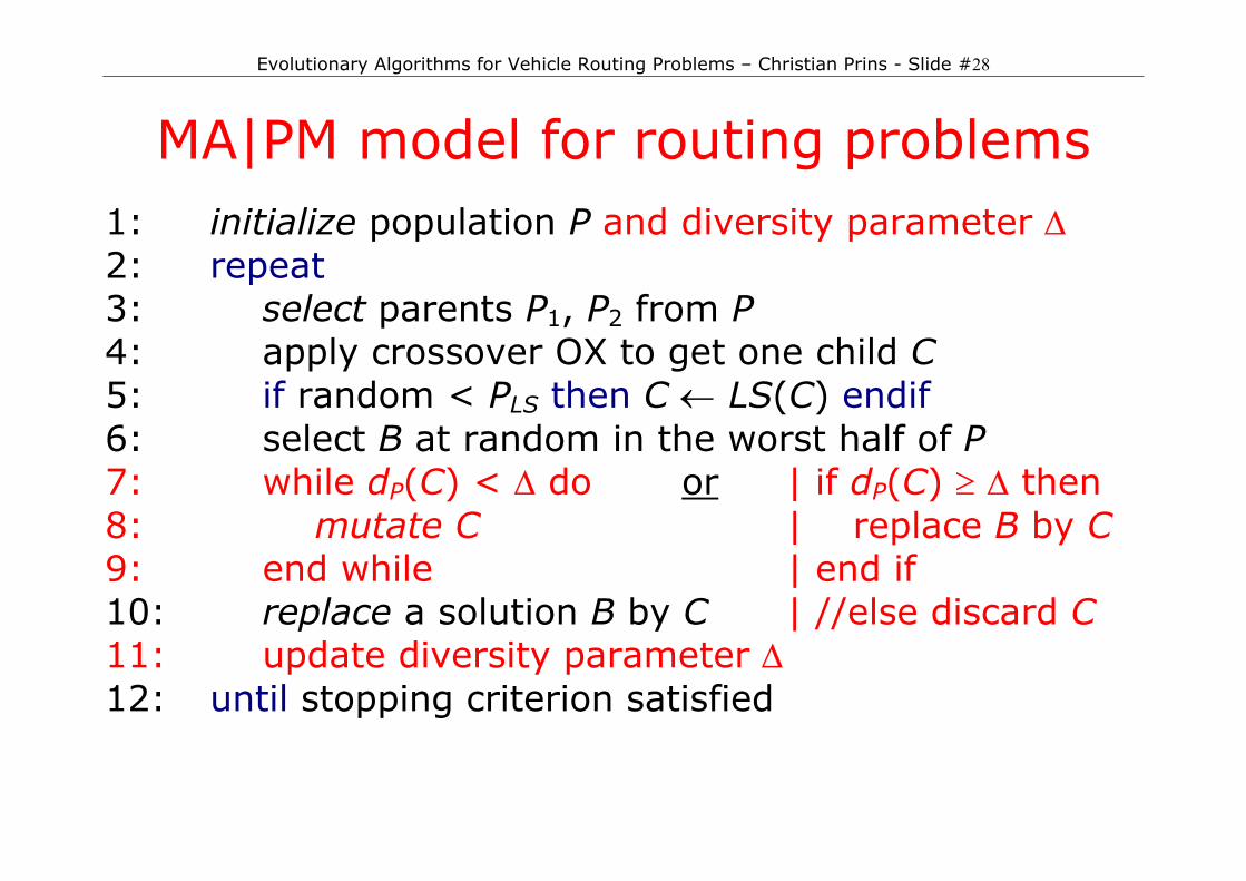
MA|PM model for routing problems

1: initialize population P and diversity parameter ∆ 2: repeat 3: select parents P1, P2 from P 4: apply crossover OX to get one child C 5: if random < PLS then C ← LS(C) endif 6: select B at random in the worst half of P 7: while dP(C) < ∆ do or | if dP(C) ≥ ∆ then 8: mutate C | replace B by C 9: end while | end if 10: replace a solution B by C | //else discard C 11: update diversity parameter ∆ 12: until stopping criterion satisfied


Some advantages of MA|PM Bridge the gap between MA and Scatter Search (SS).

Can be viewed as a "light" form of SS.

Active control of diversity thru population management.

MA-like structure: easier to implement than SS.

Easy upgrade of an existing MA.


The HVRP

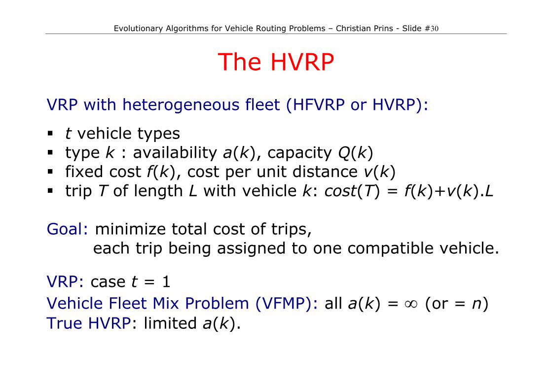
VRP with heterogeneous fleet (HFVRP or HVRP):

t vehicle types type k : availability a(k), capacity Q(k) fixed cost f(k), cost per unit distance v(k) trip T of length L with vehicle k: cost(T) = f(k)+v(k).L

Goal: minimize total cost of trips,

each trip being assigned to one compatible vehicle.

VRP: case t = 1 Vehicle Fleet Mix Problem (VFMP): all a(k) = ∞ (or = n) True HVRP: limited a(k).


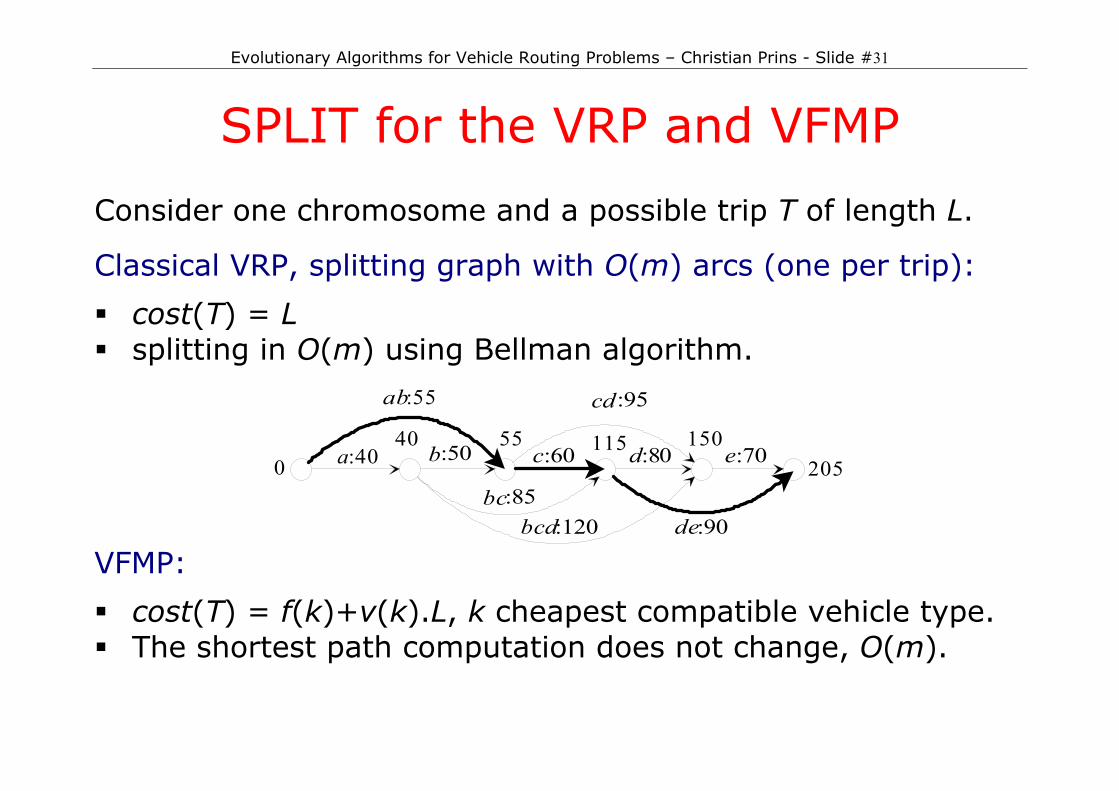
SPLIT for the VRP and VFMP Consider one chromosome and a possible trip T of length L.

Classical VRP, splitting graph with O(m) arcs (one per trip):

cost(T) = L splitting in O(m) using Bellman algorithm.

a:40 b:50 c:60 d:80 e:70

ab:55

bc:85bcd:120

cd :95

de:90

040 55 115 150

205

VFMP:

cost(T) = f(k)+v(k).L, k cheapest compatible vehicle type. The shortest path computation does not change, O(m).


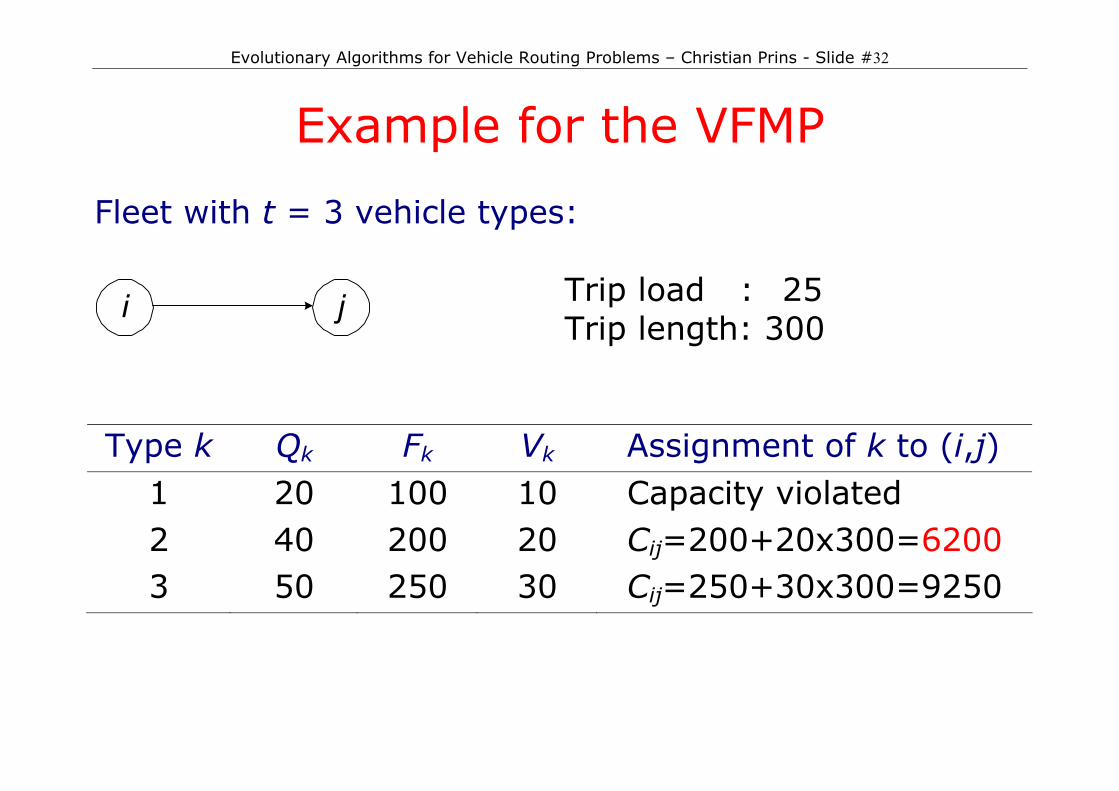
Example for the VFMP Fleet with t = 3 vehicle types:

i j

Trip load : 25 Trip length: 300

Type k Qk Fk Vk Assignment of k to (i,j)

1 20 100 10 Capacity violated 2 40 200 20 Cij=200+20x300=6200 3 50 250 30 Cij=250+30x300=9250


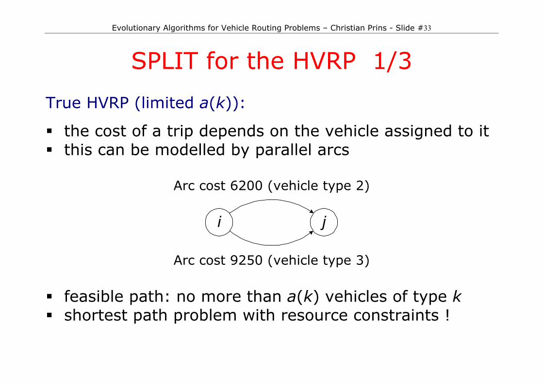
SPLIT for the HVRP 1/3 True HVRP (limited a(k)):

the cost of a trip depends on the vehicle assigned to it this can be modelled by parallel arcs

Arc cost 6200 (vehicle type 2)

i j

Arc cost 9250 (vehicle type 3) feasible path: no more than a(k) vehicles of type k shortest path problem with resource constraints !


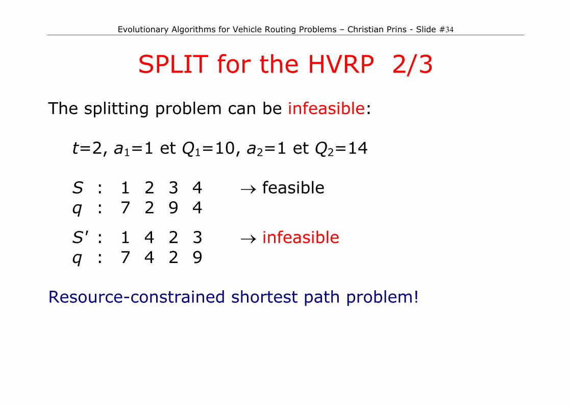
SPLIT for the HVRP 2/3 The splitting problem can be infeasible:

t=2, a1=1 et Q1=10, a2=1 et Q2=14

S : 1 2 3 4 → feasible q : 7 2 9 4

S' : 1 4 2 3 → infeasible q : 7 4 2 9

Resource-constrained shortest path problem!


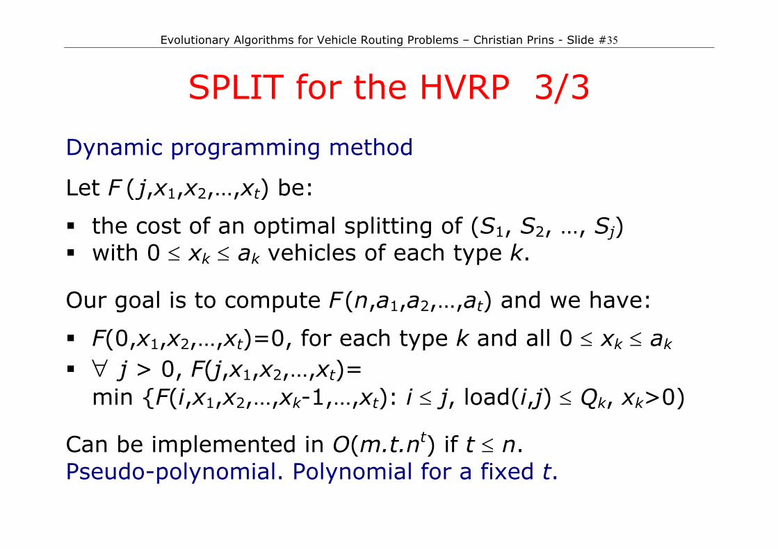
SPLIT for the HVRP 3/3 Dynamic programming method

Let F ( j,x1,x2,…,xt) be:

the cost of an optimal splitting of (S1, S2, …, Sj) with 0 ≤ xk ≤ ak vehicles of each type k.

Our goal is to compute F (n,a1,a2,…,at) and we have:

F(0,x1,x2,…,xt)=0, for each type k and all 0 ≤ xk ≤ ak

∀ j > 0, F(j,x1,x2,…,xt)= min {F(i,x1,x2,…,xk-1,…,xt): i ≤ j, load(i,j) ≤ Qk, xk>0)

Can be implemented in O(m.t.nt) if t ≤ n. Pseudo-polynomial. Polynomial for a fixed t.


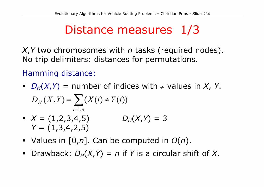
Distance measures 1/3 X,Y two chromosomes with n tasks (required nodes). No trip delimiters: distances for permutations.

Hamming distance:

DH(X,Y) = number of indices with ≠ values in X, Y.

∑=

≠=ni

H iYiXYXD,1

))()((),(

X = (1,2,3,4,5) DH(X,Y) = 3 Y = (1,3,4,2,5)

Values in [0,n]. Can be computed in O(n).

Drawback: DH(X,Y) = n if Y is a circular shift of X.


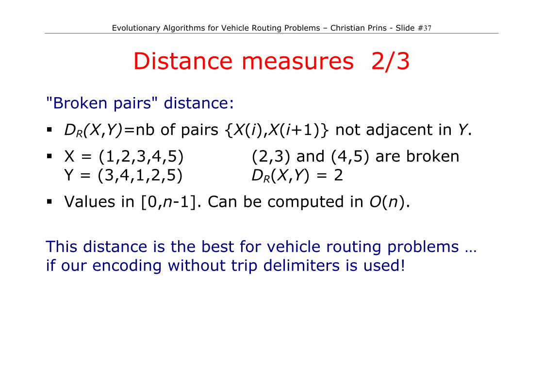
Distance measures 2/3 "Broken pairs" distance:

DR(X,Y)=nb of pairs {X(i),X(i+1)} not adjacent in Y.

X = (1,2,3,4,5) (2,3) and (4,5) are broken Y = (3,4,1,2,5) DR(X,Y) = 2

Values in [0,n-1]. Can be computed in O(n).

This distance is the best for vehicle routing problems … if our encoding without trip delimiters is used!


Distances measures 3/3

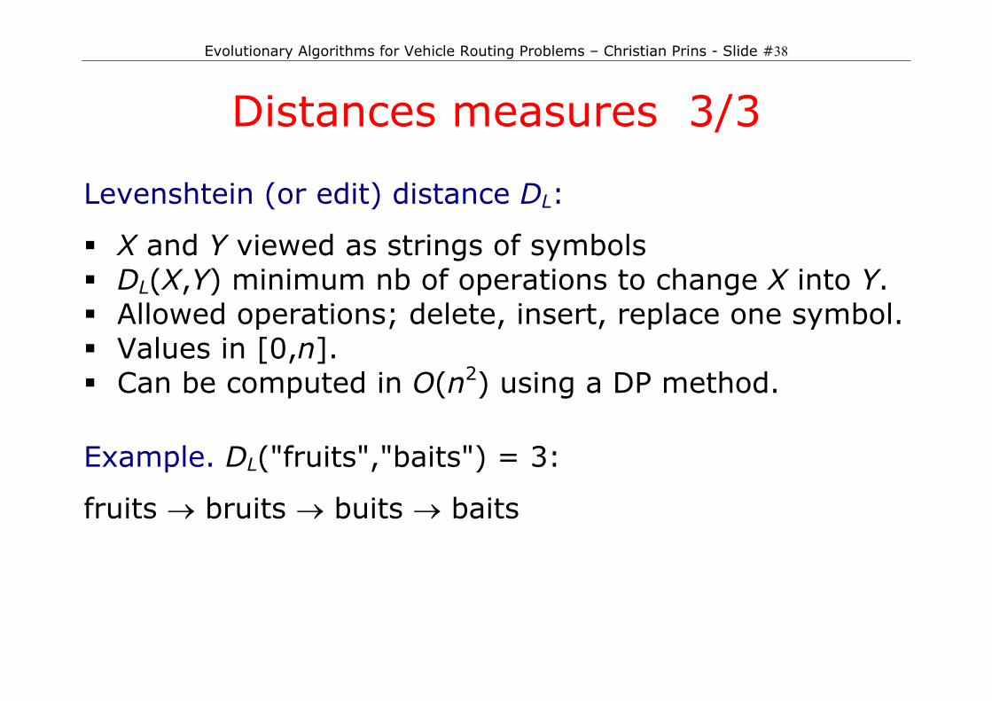
Levenshtein (or edit) distance DL:

X and Y viewed as strings of symbols DL(X,Y) minimum nb of operations to change X into Y. Allowed operations; delete, insert, replace one symbol. Values in [0,n]. Can be computed in O(n2) using a DP method.

Example. DL("fruits","baits") = 3:

fruits → bruits → buits → baits


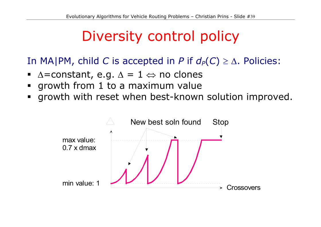
Diversity control policy In MA|PM, child C is accepted in P if dP(C) ≥ ∆. Policies: ∆=constant, e.g. ∆ = 1 ⇔ no clones growth from 1 to a maximum value growth with reset when best-known solution improved.

Crossoversmin value: 1

max value:0.7 x dmax

New best soln found Stop


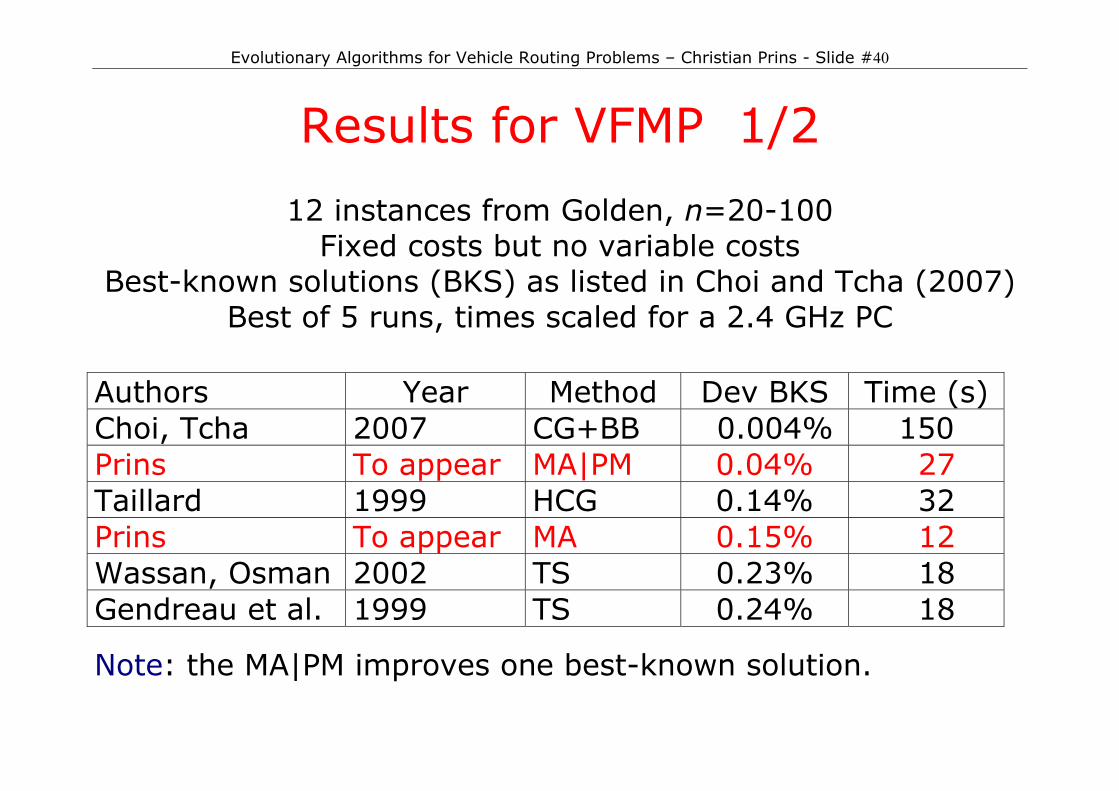
Results for VFMP 1/2

12 instances from Golden, n=20-100 Fixed costs but no variable costs

Best-known solutions (BKS) as listed in Choi and Tcha (2007) Best of 5 runs, times scaled for a 2.4 GHz PC

Authors Year Method Dev BKS Time (s) Choi, Tcha 2007 CG+BB 0.004% 150 Prins To appear MA|PM 0.04% 27 Taillard 1999 HCG 0.14% 32 Prins To appear MA 0.15% 12 Wassan, Osman 2002 TS 0.23% 18 Gendreau et al. 1999 TS 0.24% 18

Note: the MA|PM improves one best-known solution.


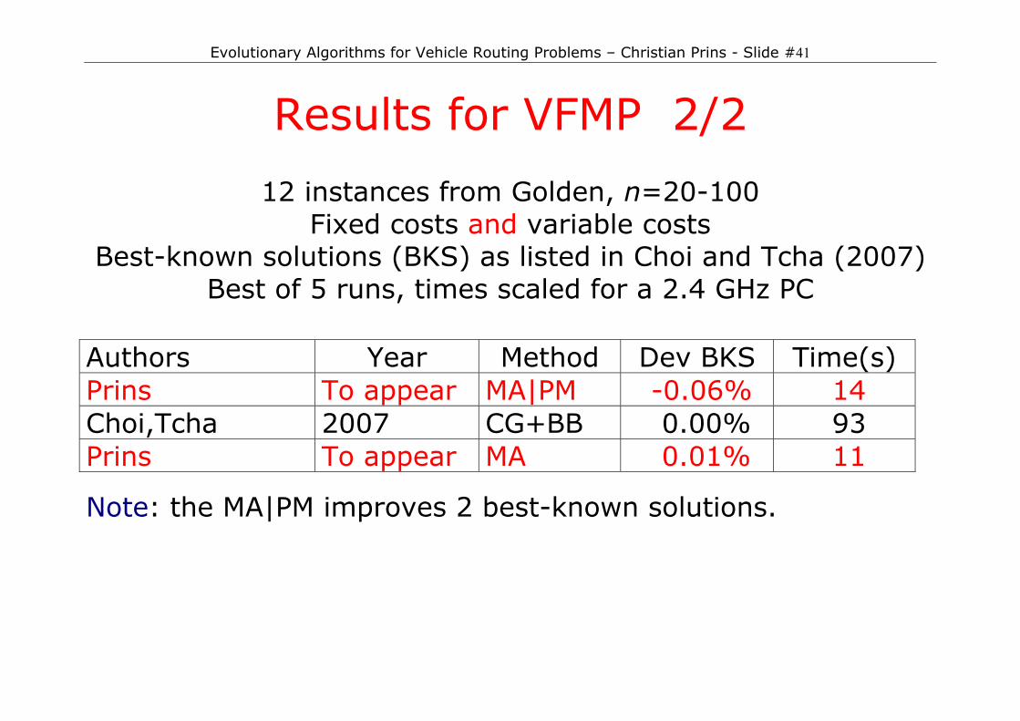
Results for VFMP 2/2

12 instances from Golden, n=20-100 Fixed costs and variable costs

Best-known solutions (BKS) as listed in Choi and Tcha (2007) Best of 5 runs, times scaled for a 2.4 GHz PC

Authors Year Method Dev BKS Time(s) Prins To appear MA|PM -0.06% 14 Choi,Tcha 2007 CG+BB 0.00% 93 Prins To appear MA 0.01% 11

Note: the MA|PM improves 2 best-known solutions.


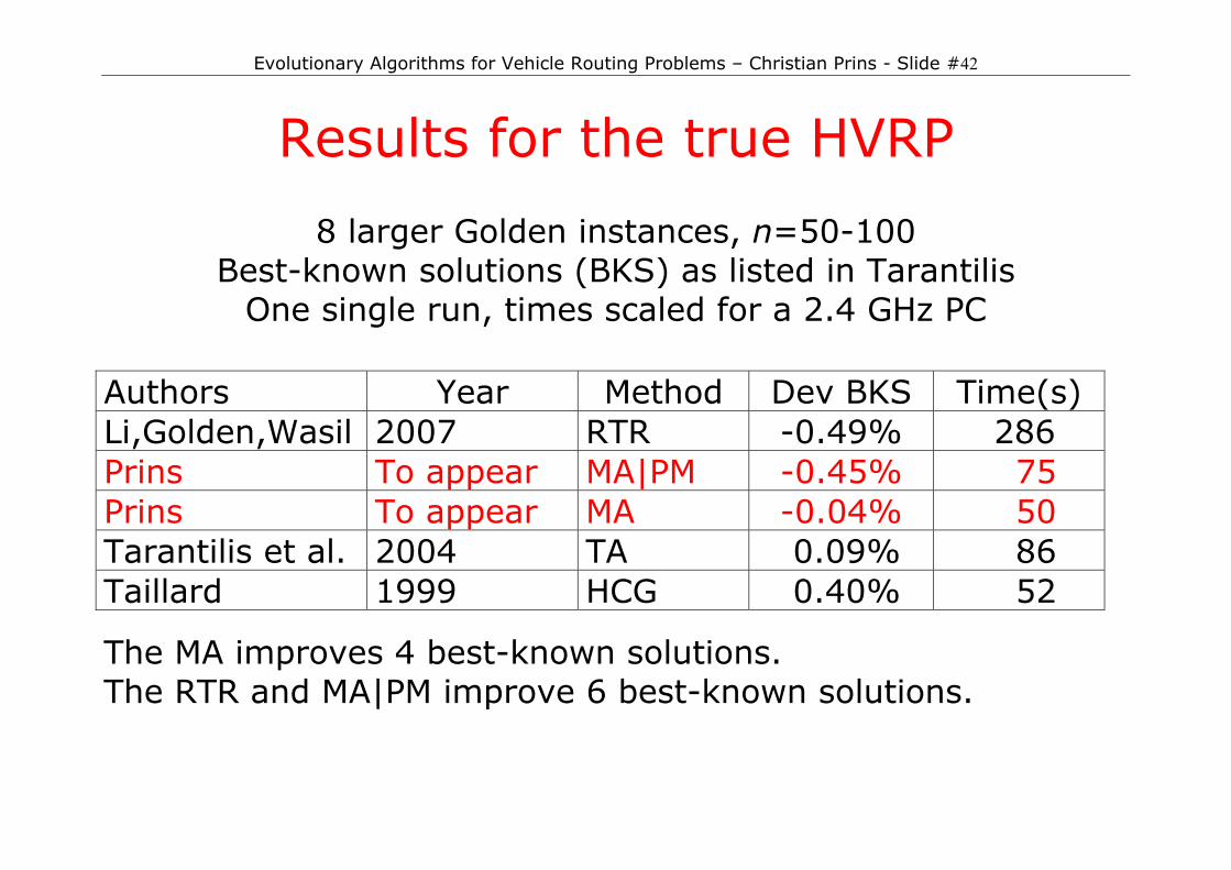
Results for the true HVRP

8 larger Golden instances, n=50-100 Best-known solutions (BKS) as listed in Tarantilis

One single run, times scaled for a 2.4 GHz PC Authors Year Method Dev BKS Time(s) Li,Golden,Wasil 2007 RTR -0.49% 286 Prins To appear MA|PM -0.45% 75 Prins To appear MA -0.04% 50 Tarantilis et al. 2004 TA 0.09% 86 Taillard 1999 HCG 0.40% 52

The MA improves 4 best-known solutions. The RTR and MA|PM improve 6 best-known solutions.


References N. Labadi, P. Lacomme, C. Prins, A memetic algorithm for the heterogeneous fleet VRP, Proceedings of Odysseus 2006, E. Benavent et al. (Eds.), pp. 209-213, Univ. of Valencia, 2006.

C. Prins, Two memetic algorithms for vehicle routing problems with heterogeneous fleets, Engineering Applications of Artificial Intelligence, forthcoming.


PART 4

Periodic problems


The Periodic VRP - Basic version

PVRP data: undirected graph G, depot + n required nodes (tasks) planning horizon H of np periods or "days" for each task i, frequency f(i) (number of visits in H) demands q(i), service times s(i), travel times C(i,j).

Goal (hierarchical bi-objective function): select f(i) days per task i and solve one VRP per day main objective: minimize fleet size secondary objective: total duration of trips over H

Applications: industrial waste collection, drinks dispensers, delivery of propane to glass houses etc.


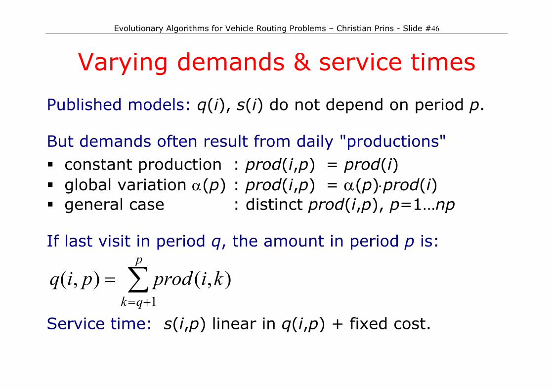
Varying demands & service times Published models: q(i), s(i) do not depend on period p. But demands often result from daily "productions" constant production : prod(i,p) = prod(i) global variation α(p) : prod(i,p) = α(p)⋅prod(i) general case : distinct prod(i,p), p=1…np

If last visit in period q, the amount in period p is:

∑+=

=p

qkkiprodpiq

1),(),(

Service time: s(i,p) linear in q(i,p) + fixed cost.


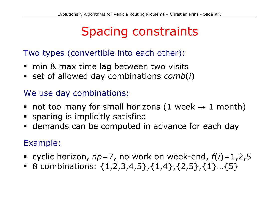
Spacing constraints Two types (convertible into each other):

min & max time lag between two visits set of allowed day combinations comb(i)

We use day combinations:

not too many for small horizons (1 week → 1 month) spacing is implicitly satisfied demands can be computed in advance for each day

Example:

cyclic horizon, np=7, no work on week-end, f(i)=1,2,5 8 combinations: {1,2,3,4,5},{1,4},{2,5},{1}…{5}


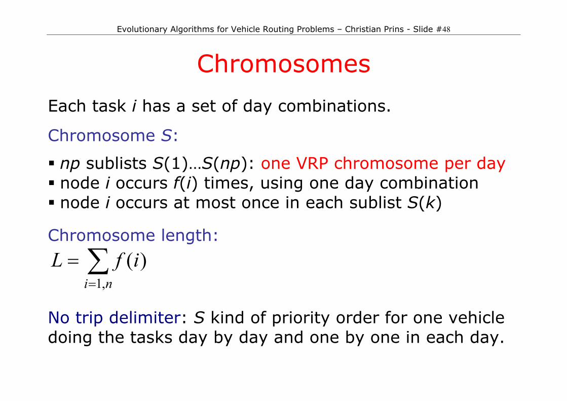
Chromosomes Each task i has a set of day combinations.

Chromosome S:

np sublists S(1)…S(np): one VRP chromosome per day node i occurs f(i) times, using one day combination node i occurs at most once in each sublist S(k)

Chromosome length:

∑=

=niifL

,1)(

No trip delimiter: S kind of priority order for one vehicle doing the tasks day by day and one by one in each day.


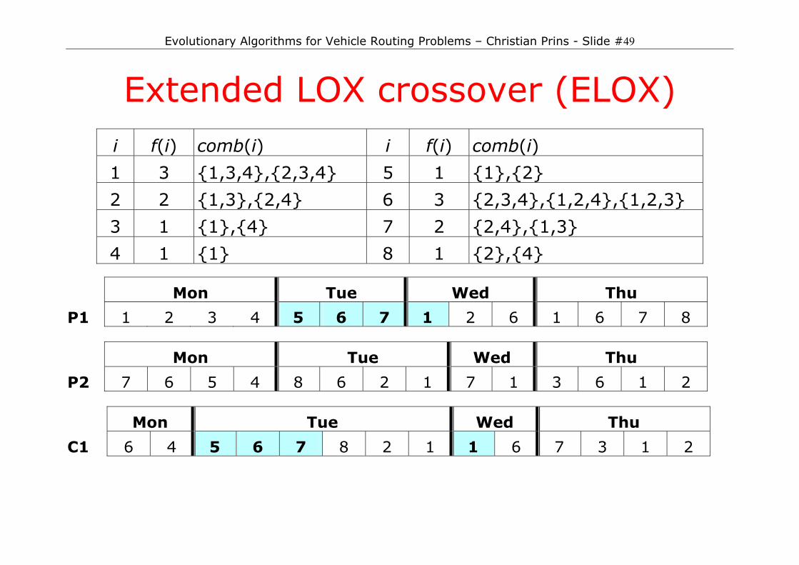
Extended LOX crossover (ELOX)

i f(i) comb(i) i f(i) comb(i)

1 3 {1,3,4},{2,3,4} 5 1 {1},{2}

2 2 {1,3},{2,4} 6 3 {2,3,4},{1,2,4},{1,2,3}

3 1 {1},{4} 7 2 {2,4},{1,3}

4 1 {1} 8 1 {2},{4}

Mon Tue Wed Thu

P1 1 2 3 4 5 6 7 1 2 6 1 6 7 8

Mon Tue Wed Thu

P2 7 6 5 4 8 6 2 1 7 1 3 6 1 2

Mon Tue Wed Thu

C1 6 4 5 6 7 8 2 1 1 6 7 3 1 2


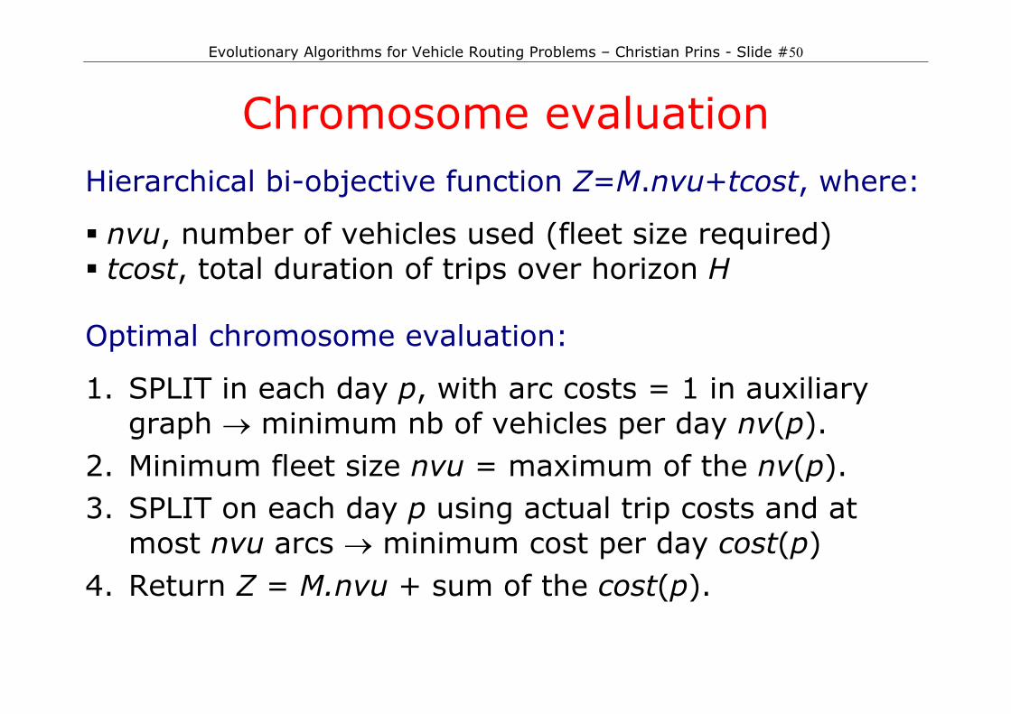
Chromosome evaluation

Hierarchical bi-objective function Z=M.nvu+tcost, where:

nvu, number of vehicles used (fleet size required) tcost, total duration of trips over horizon H

Optimal chromosome evaluation:

1. SPLIT in each day p, with arc costs = 1 in auxiliary graph → minimum nb of vehicles per day nv(p).

2. Minimum fleet size nvu = maximum of the nv(p). 3. SPLIT on each day p using actual trip costs and at

most nvu arcs → minimum cost per day cost(p) 4. Return Z = M.nvu + sum of the cost(p).


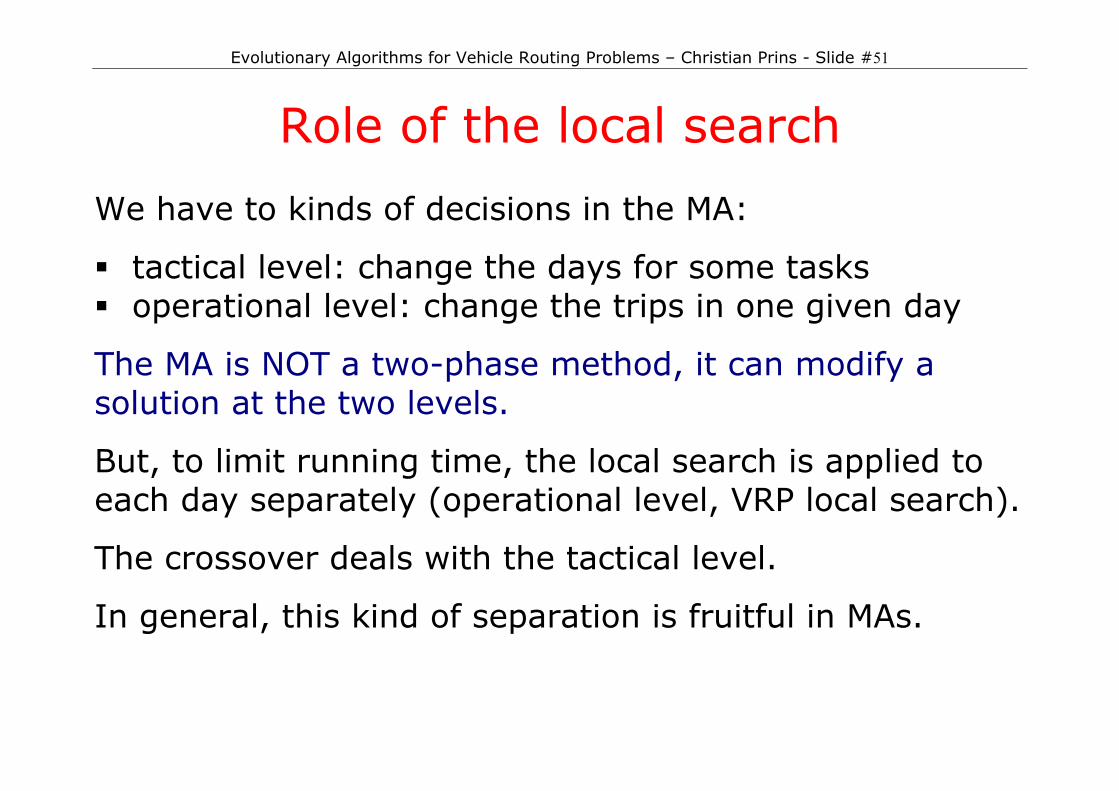
Role of the local search We have to kinds of decisions in the MA:

tactical level: change the days for some tasks operational level: change the trips in one given day

The MA is NOT a two-phase method, it can modify a solution at the two levels.

But, to limit running time, the local search is applied to each day separately (operational level, VRP local search).

The crossover deals with the tactical level.

In general, this kind of separation is fruitful in MAs.


References The method was developed in fact for the periodic capacitated arc routing problem (PCARP) but the algorithm is easily transposed to the PVRP: P. Lacomme, C. Prins, W. Ramdane-Chérif: Evolutionary algorithms for periodic arc routing problems, EJOR, 165(2), pp. 535-553, 2005. F. Chu, N. Labadi, C. Prins: Heuristics for the periodic capacitated arc routing problem, Journal of Intelligent Manufacturing, 16(2), pp. 243-251, 2005.


Concluding remarks Memetic algorithms are effective tools to solve vehicle routing problems. The SPLIT procedure is general and flexible… as long as the shortest path problem is polynomial (VRP, VRPTW, PVRP) or pseudo-polynomial (HVRP)! Software engineering point of view: the progressive upgrade GA → MA → MA|PM is (relatively) easy. Remarks confirmed by other applications not described here (e.g. time windows, multi-objective problems).

Documents

Evolutionary Algorithms for Vehicle Routing · PDF fileEvolutionary Algorithms for Vehicle Routing Problems ... Evolutionary Algorithms for Vehicle Routing Problems ... TS Osman 1993